Estimation of Social Interaction Models: A Bayesian Approach

Estimation of Social Interaction Models: ABayesian Approach

Paula AlmonacidI Network Métodos Cuantitativos

November 14, 2017

Outline1 Introduction

Social interaction models

2 Likelihood function

3 Bayesian approachJoint prior distributionJoint posterior distributionConditional posterior distributionsSimulation settingSimulation settingSimulation results

4 Empirical ApplicationValue in Financial Communities

3






4

Introduction

Definition

What is aneighbor-

hood effect?

Sociology Economics Spatial Economet.

Political Im-plications

5

Introduction

Types of effects

Classificationof the models

Geography Scope Spatial Delineation

Endogenous Correlation Exogenous

6

Introduction

Empirical estimation challengesEndogenous and omitted independent variables.Identification of particular kind of effect may not be possibleDepending on how the characteristics of the individualsvary with the characteristics of their neighborhood.

7

Introduction

Lee (2007) proposed the following specification for the SARmodel:

Yg = λWgYg + Xg,1β1 + WgXg,2β2 + 1mgαg + εg (1)

εg ∼ Nmg (0, σ2Img ) (2)

8

Introduction

Yg = (yg,1, · · · , yg,mg )′ is a vector of endogenous variables.Xg is the matrix of exogenous variables of dimensionmg × K .1mg is a vector of ones of dimension of mg × 1.αg are unobserved group specific effects.Wg is the social interaction matrix. Each of its entries willtake value 1 if there is a link and 0 otherwise.

9

IntroductionStructure of the modelThe observational units of the model are individuals, which aredenoted by iThese individuals are grouped into a single group denoted gThe composition of the group is established before the statisticalexerciseThe specification of the interactions of each group isrepresenting by the matrix Wg

The interaction of all groups could also be represented into onebig matrix, which is a block diagonal matrix.

10

Introduction

Wg =1

mg − 1(1mg 1′mg

− Img ) g = 1, . . . ,G (3)

where 1mg is the mg-dimensional column vector of ones, and Img

is the mg-dimensional identity matrix. Equivalently, in terms ofeach unit i from a group g,

11

Introduction

In terms of each unit i from a group g,

Yg = λ

1mg − 1

mg∑j=1,j 6=i

yg,j

+x ′g,i,1β1+

1mg − 1

mg∑j=1,j 6=i

x ′g,j,2β2

+αg+εg,i

(4)

12






13

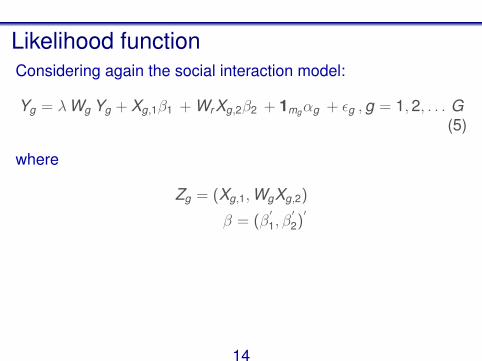
Likelihood functionConsidering again the social interaction model:

Yg = λWg Yg + Xg,1β1 + Wr Xg,2β2 + 1mgαg + εg ,g = 1,2, . . . G(5)

where

Zg = (Xg,1,WgXg,2)

β = (β′

1, β′

2)′

14

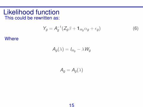
Likelihood functionThis could be rewritten as:

Yg = A−1g (Zgβ + 1mgαg + εg) (6)

Where

Ag(λ) = Img − λWg

Ag = Ag(λ)

15

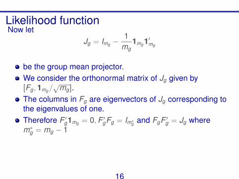
Likelihood functionNow let

Jg = Img −1

mg1mg 1′mg

be the group mean projector.We consider the orthonormal matrix of Jg given by[Fg,1mg/

√mg].

The columns in Fg are eigenvectors of Jg corresponding tothe eigenvalues of one.Therefore F ′g1mg = 0,F ′gFg = Im∗g and FgF ′g = Jg wherem∗g = mg − 1

16

Pre-multiplication of the equation (6) by F ′g leads to the followingtransformed model without α′gs

(F ′gAgFg)(F ′gYg) = (F ′gZgβ) + (F ′gεg)

A∗gY ∗g = Z ∗gβ + ε∗g

whereA∗g = (F ′gAgFg)

Y ∗g = (F ′gYg)

ε∗g = (F ′gεg)

17

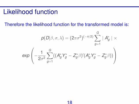
Likelihood function

Therefore the likelihood function for the transformed model is:

p(D|β, σ, λ) = (2πσ2)(−n/2)G∑

g=1

| A∗g | ×

exp

− 12σ2

G∑g=1

((A∗gY ∗g − Z ∗gβ)′(A∗gY ∗g − Z ∗gβ))

18






19

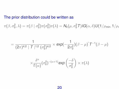
The prior distribution could be written as

π(β, σ20, λ) = π(β | σ2

0)π(σ20)π(λ) = Nk (µ, σ2

0T )IG(α, δ)U(1/ρmin,1/ρmax )

=1

(2π)k |2 | T |1|2 (σ20)k |2 × exp(− 1

2σ20

)(β − µ)′T−1(β − µ)

× δα

Γ(α)(σ2

0)−(α+1)exp(−δσ2

0

)× π(λ)

20

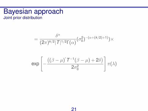
Bayesian approachJoint prior distribution

=δα

(2π)k/2|T |1/2Γ(α)(σ2

0)−(α+(k/2)+1))×

exp

[−((β − µ)

′T−1(β − µ) + 2δ)

2σ20

]π(λ)

21

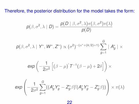
Therefore, the posterior distribution for the model takes the form:

p(β, σ2, λ | D) =p(D | β, σ2, λ)π(β, σ2)π(λ)

p(D)

p(β, σ2, λ | Y ∗,W ∗,Z ∗) ∝ (σ2)−(α∗+(k/2)+1)

G∑g=1

| A∗g | ×

exp(− 1

2σ2

[(β − µ)

′T−1(β − µ) + 2δ

])×

exp

− 12σ2

G∑g=1

((A∗gY ∗g − Z ∗gβ)′(A∗gY ∗g − Z ∗gβ))

× π(λ)

22

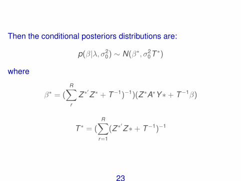
Then the conditional posteriors distributions are:

p(β|λ, σ20) ∼ N(β∗, σ2

0T ∗)

where

β∗ = (R∑r

Z ∗′Z ∗ + T−1)−1)(Z ∗A∗Y∗+ T−1β)

T ∗ = (R∑

r=1

(Z ∗′Z∗+ T−1)−1

23

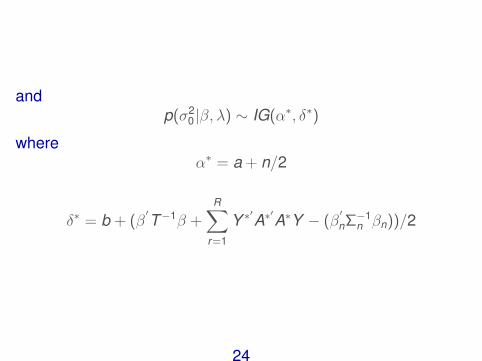
andp(σ2

0|β, λ) ∼ IG(α∗, δ∗)

whereα∗ = a + n/2

δ∗ = b + (β′T−1β +

R∑r=1

Y ∗′A∗′A∗Y − (β

′

nΣ−1n βn))/2

24

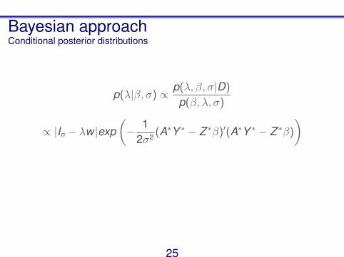
Bayesian approachConditional posterior distributions

p(λ|β, σ) ∝ p(λ, β, σ|D)

p(β, λ, σ)

∝ |In − λw |exp(− 1

2σ2 (A∗Y ∗ − Z ∗β)′(A∗Y ∗ − Z ∗β)

)

25

Simulation settingAll groups are assumed to have different sizes (between: 2and 10, 2 and 15, 2 and 30, and, 2 and 50).The number of groups are set to 67 and 102.The data generating process are specified as follows :λ = 0.5, β11 = 1, β12 = −1, β21 = 1, β22 = −1 and σ = 1.The data generation process for each of the Xg variables isNmg (0, Img )

The continuous dependent variable Yg can be directlygenerated based on the model.The number of simulations are 100.

26

Bayesian ApproachSimulation setting

In particular, we use vague prior distributions settingβ0 = 0,Σ = diag(1000), α = 0.001 and δ = 0.001.We sampled directly β and σ2

0 from Gibbs sampling stepssince their posterior conditional distributions have closedformsNevertheless, we use the Metropolis–Hastings (M–H)algorithm for sampling the social interaction parameter λbecause the full conditional distribution for λ is nonstandarddue to the presence of Wr .

27

Group size Num gr. Approach Lambda Beta_11 Beta_12 Beta_21 Beta_22 Sigma

2 to 10

67ML 0.3344 0.0796 0.0850 0.2546 0.2677 0.0687

Bayes 0.2405 0.0626 0.0747 0.2647 0.2743 0.0599

102ML 0.2565 0.0588 0.0677 0.1771 0.2080 0.0523

Bayes 0.1911 0.0519 0.0534 0.2199 0.1981 0.0510

2 to 15

67ML 0.3138 0.0559 0.0590 0.2975 0.3413 0.0480

Bayes 0.2156 0.0554 0.0508 0.2752 0.2871 0.0395

102ML 0.2297 0.0476 0.0480 0.2526 0.2463 0.0375

Bayes 0.1906 0.0466 0.0434 0.2166 0.2388 0.0321

2 to 30

67ML 0.3435 0.0416 0.0411 0.3438 0.3469 0.0346

Bayes 0.2226 0.0326 0.0330 0.3678 0.3506 0.0267

102ML 0.2961 0.0287 0.0286 0.2871 0.2949 0.0240

Bayes 0.2030 0.0311 0.0266 0.2725 0.2897 0.0240

2 to 50

67ML 0.4567 0.0326 0.0257 0.4665 0.4176 0.0214

Bayes 0.2276 0.0264 0.0276 0.4346 0.4604 0.0188

102ML 0.3319 0.0251 0.0239 0.3666 0.3374 0.0175

Bayes 0.1878 0.0195 0.0218 0.3580 0.3201 0.0151

28

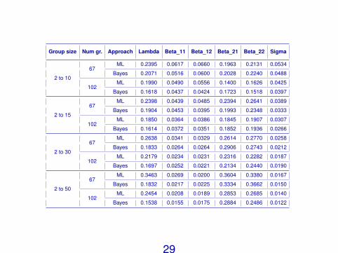
Group size Num gr. Approach Lambda Beta_11 Beta_12 Beta_21 Beta_22 Sigma

2 to 10

67ML 0.2395 0.0617 0.0660 0.1963 0.2131 0.0534

Bayes 0.2071 0.0516 0.0600 0.2028 0.2240 0.0488

102ML 0.1990 0.0490 0.0556 0.1400 0.1626 0.0425

Bayes 0.1618 0.0437 0.0424 0.1723 0.1518 0.0397

2 to 15

67ML 0.2398 0.0439 0.0485 0.2394 0.2641 0.0389

Bayes 0.1904 0.0453 0.0395 0.1993 0.2348 0.0333

102ML 0.1850 0.0364 0.0386 0.1845 0.1907 0.0307

Bayes 0.1614 0.0372 0.0351 0.1852 0.1936 0.0266

2 to 30

67ML 0.2638 0.0341 0.0329 0.2614 0.2770 0.0258

Bayes 0.1833 0.0264 0.0264 0.2906 0.2743 0.0212

102ML 0.2179 0.0234 0.0231 0.2316 0.2282 0.0187

Bayes 0.1697 0.0252 0.0221 0.2134 0.2440 0.0190

2 to 50

67ML 0.3463 0.0269 0.0200 0.3604 0.3380 0.0167

Bayes 0.1832 0.0217 0.0225 0.3334 0.3662 0.0150

102ML 0.2454 0.0208 0.0189 0.2853 0.2685 0.0140

Bayes 0.1538 0.0155 0.0175 0.2884 0.2486 0.0122

29






30

Empirical ApplicationIntroduction

One interesting application for this type of models is bankprofitability.The role of banks remains central in various importantaspects for the economyMost of studies on bank profitability, estimate the impact ofnumerous factors that may be important in explaining profitsusing linear modelsEven though these studies show that it is possible toconduct a meaningful analysis of bank profitability, there arestill some issues to be addressed.

31

Empirical ApplicationValue in Financial Communities

Model SpecificationTherefore, we propose the following model specification:

Profitg = λWgProfitg + CashFgβ1 + WorKCgβ2 + Leveragegβ3

+EBITDAintβ4 + ROAβ5 + WgCashFgβ6 + WgWorkCgβ7

+WgLeveragegβ8 + WgEBITDAintgβ9 + WgROAgβ10 + lmgαg + εg

32

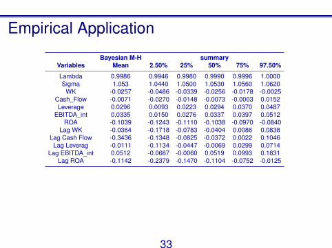
Empirical Application

Bayesian M-H summaryVariables Mean 2.50% 25% 50% 75% 97.50%

Lambda 0.9986 0.9946 0.9980 0.9990 0.9996 1.0000Sigma 1.053 1.0440 1.0500 1.0530 1.0560 1.0620

WK -0.0257 -0.0486 -0.0339 -0.0256 -0.0178 -0.0025Cash_Flow -0.0071 -0.0270 -0.0148 -0.0073 -0.0003 0.0152Leverage 0.0296 0.0093 0.0223 0.0294 0.0370 0.0487

EBITDA_int 0.0335 0.0150 0.0276 0.0337 0.0397 0.0512ROA -0.1039 -0.1243 -0.1110 -0.1038 -0.0970 -0.0840

Lag WK -0.0364 -0.1718 -0.0783 -0.0404 0.0086 0.0838Lag Cash Flow -0.3436 -0.1348 -0.0825 -0.0372 0.0022 0.1046

Lag Leverag -0.0111 -0.1134 -0.0447 -0.0069 0.0299 0.0714Lag EBITDA_int 0.0512 -0.0687 -0.0060 0.0519 0.0993 0.1831

Lag ROA -0.1142 -0.2379 -0.1470 -0.1104 -0.0752 -0.0125

33

We welcome your comments, questions, and suggestions.Thank you!!!

34

Estimation of Social Interaction Models: A Bayesian Approach

Economy & Finance

Transcript of Estimation of Social Interaction Models: A Bayesian Approach