Estimation of rating class transitionprobabilities with incomplete data

Thomas Mählmann

Chair of Banking, University of Cologne

Albertus-Magnus-Platz

50923 Koeln/Germany

Tel: (0049)+221-4702628

Fax: (0049)+221-4702305

maehlmann@wiso.uni-koeln.de

Estimation of rating class transitionprobabilities with incomplete data

Abstract

This paper shows that the well known �duration� and �cohort� methods for estimating tran-

sition probabilities of external bond ratings are not suitable for internal rating data. More pre-

cisely, the duration method cannot and the cohort method should not be used in connection with

bank rating data. Structural differences within the borrower monitoring process of banks and rat-

ing agencies are responsible for this result. A Maximum Likelihood (ML) estimation procedure,

which accounts for the peculiarities of internal bank ratings, is introduced and applied to data from

a German bank. The empirical results indicate that the differences between cohort and ML transi-

tion matrices are both, statistically and economically signi�cant. Furthermore, evidence of rating

reversals, business cycle dependent transition probabilities and on the factors which determine the

borrower monitoring intensity of banks is provided.

Key words: internal ratings, transition probabilities, Markov process, borrower monitoring

JEL classi�cation codes: C24, C41, G21, G28

1

1 Introduction

Over the past few years, banks have attempted to mirror the rating behavior of external rating agen-

cies. But, are internal and external rating procedures really very similar? Or, more speci�cally, can

methods developed for external ratings (e.g. migration probability estimation or validation tech-

niques) be applied to internal bank ratings? This paper tries to provide answers to these questions

in the context of migration risk, i.e. the probability of moving from one rating class to another

within a given amount of time.

At �rst sight, the estimation of the migration or transition probability matrix for internal ratings

seems to be an easy task in face of the methodology already available for estimating transition

probabilities of external bond ratings. However, as will be seen, there is at least one fundamental

difference between external and internal rating data which prevents the transfer of the methods

developed for agency ratings. In particular, we argue that internal ratings are not continuously

monitored and so internal rating data is discrete, i.e. observations are taken at speci�ed time

points. In the absence of continuous monitoring, a borrower could change credit grade without

anyone noticing. Moreover, banks frequently base the decision of when to monitor a borrower on

an estimate of the borrowers expected loss (see Basel Committee on Banking Supervision, 2000,

or Treacy and Carey, 2000). For example, borrowers with cash-collateralized loans or borrowers

in higher-quality grades may receive a refreshed rating only once every two years whereas low-

quality borrowers may be reviewed several times within one year. In sum, internal rating data can

be characterized by two important features: (i) Exact times of movement between rating classes

and the class occupancy in between the observation times are unknown and (ii) observation and

interexamination times vary for different borrowers.

The traditional discrete �cohort� or �multinomial� type estimator as well as the continuous

�duration� estimator (see Jafry and Schuermann, 2004, or Lando and Skødeberg, 2002) are not

capable to deal appropriately with such data. In concrete terms, the �rst data feature prevents the

application of the duration approach and the second feature brings about an ef�ciency loss for

the cohort estimator. Therefore, an alternative estimation method that is suitable for incompletely

observed rating data is proposed and applied to data from a German bank. This method derives

ML estimates of transition probabilities under the assumption that rating dynamics follow a time-

homogeneous �rst-order Markov process.

2

The empirical part of this paper studies the following three questions: (i) Which factors in�u-

ence the monitoring intensity of bank borrowers? (ii) Are cohort and ML estimates of transition

probabilities statistically and economically distinguishable? (iii) Can the process underlying inter-

nal rating changes be described as a time-homogeneous �rst-order Markov process?

Concerning the �rst question, our evidence suggests that the more favorable the current rating

the greater, ceteris paribus, the probability for a review within less than a one-year period. This

somewhat surprising �nding might be explained by agency issues between the lending of�cer in

the bank and senior management. Furthermore, a previous upgrade pattern and a longer duration

of the bank-borrower relationship reduce the review frequency, and the effect of borrower size is

U-shaped.

With respect to one-year transition probability matrices, it seems to be that two countervailing

effects drive the differences between the ML and the cohort estimates: A duration dependence

effect states an inversely U-shaped relation among the time between two subsequent monitoring

steps and the probability of a rating change, and a downgrade effect re�ects the empirical obser-

vation (see Lando and Skødeberg, 2002) that defaulted borrowers are frequently downgraded to

the highest risk class shortly before they actually default. Taking both effects together results in a

small, but statistically and economically signi�cant value for the distance metric proposed by Jafry

and Schuermann (2004) for comparing migration matrices.

Finally, by using a form of a proportional hazard model we �nd evidence for business cycle

in�uence on rating intensities and for rating reversals, i.e. an upgrade followed by a downgrade,

or a downgrade followed by an upgrade. Such rating bounces are consistent with the assumption

of Gaussian distributed credit quality changes in structural models of rating transitions (Gordy

and Heit�eld, 2001, or Löf�er, 2005). However, business cycle dependence and rating reversals

undermine the assumptions of any of the estimators discussed above and thus leave open some

important questions for future research on the analysis of internal ratings.

The paper proceeds as follows. Section 2 points out key differences between what we are used

to seeing, i.e. histories of agency ratings, and bank data. In section 3, a regression analysis is

performed to characterize the speci�c nature of internal rating data from a German bank. The new

generator-based ML transition probability estimator is described in section 4 and compared to the

widely applied cohort estimator in section 5. The paper concludes with section 6.

3

2 Structure of internal rating data

Obviously, before estimating transition probabilities one should ask whether all transitions made

by a single borrower over a speci�ed observation period and the corresponding exact transition

times are known. Or, in short, whether the rating data is continuous or discrete. To answer this

question for the kind of data that can be obtained from agencies and banks, the monitoring intensity

of both has to be analyzed.

Regarding rating agencies, it seems reasonable to expect that their data is on a approximately

continuous scale, i.e. roughly exact transition times are available.1 Agencies are able to perform

almost a continuous monitoring mainly for two reasons. First, they typically rate only large pub-

lic �rms which do regularly issue �xed income securities. These �rms are forced to disclose a

considerable amount of information, which is digested and �ltered by many market participants.

Moreover, since agencies are directly paid by the issuers of debt, they can spend substantial re-

sources on discovering and updating private information.

In contrast, commercial banks are faced with a different situation. They have to rate a bulk

of small and middle-market loans and the costs of producing ratings must be covered by revenues

on credit products. The expenditure of resources at a rate similar to that of the rating agencies

would make the business with small and middle-market loans unpro�table. In addition, monitoring

private �rms with poor and infrequent information is much more costly. Therefore, to reduce costs

banks are forced to perform a formal review of each rating on an annual basis only. However,

Machauer and Weber (1998) report that the time between two consecutive monitoring processes

does not always equal one year in their sample. Indeed, it seems to be common practice to base the

decision about the frequency of reviews on the current rating or the collateral (see Basel Committee1Note that even rating agencies do not perform a truly continuous monitoring. This can be seen from the existence

of watchlists, which are of no use if all issuers were under a continuous review anyway. In addition, rating agencies

are often accused of being too slow to adjust their ratings. For example, empirical evidence by Delianedis and Geske

(1999) shows that rating changes lag changes in default probabilities. A possible reason for not reporting exact

transition times is the agency's �rating reversal aversion� (see Löf�er, 2005). A continuous monitoring, however,

does not imply that ratings are changed every time new information is obtained. According to their �through-the-

cycle� point of view external ratings are stable because they are intended to measure default risk over long investment

horizons, and thus they are changed only when agencies are con�dent that observed changes in a �rm's risk pro�le are

likely to be permanent.

4

on Banking Supervision, 2000, p. 37, Treacy and Carey, 2000, p. 182). In addition, the theoretical

work of Diamond (1989, 1991) suggests that holding credit risk constant, monitoring and borrower

reputation are close substitutes. Then, as �rms successfully complete loan transactions with banks

and thus acquire reputation, banks monitor them less frequently and, ultimately, charge them lower

interest rates. Blackwell and Winters (1997) provide empirical evidence that banks less frequently

monitor �rms with whom they have closer relationships.

From the preceding arguments we might conclude that in almost all cases internal rating data

will be discrete and the choice of the observation times depends on: (i) The current rating (re�ects

the probability of default, PD), (ii) the terms of the loan (re�ect the loss given default, LGD), (iii)

the loan size (re�ects the exposure at default, EAD) and (iv) the closeness of the bank-borrower re-

lationship (re�ects the moral hazard component of credit risk). Thus the structure of the monitoring

times will vary for each borrower, depending on his level of expected loss (EL=PD�LGD�EAD).2

3 Empirical analysis of monitoring intensities

3.1 The data

Our data comes from the internal rating system of a medium-sized German bank. This rating sys-

tem is composed of two parts: A quantitative subrating, called �nancial rating, and a qualitative

subrating, called corporate situation rating. As opposed to the corporate situation rating, which

relies on a subjective assessment of qualitative criteria (e.g. market position, management quality

etc.), the �nancial rating is based on a statistical model, which essentially combines ratio analysis

and industry sector information. The overall rating results by applying the subjectively determined,

�xed weights 0.7 and 0.3 to the �nancial and corporate situation subratings, respectively. The bank

provided us with the rating history of all borrowers in its loan portfolio as at January 31, 2002, that

did not default by the end of that year. In addition, rating information for all borrowers which de-

faulted within the period 1996-2002 is obtained. Here legal bankruptcy proceedings and loan loss2It should be noted that the Basel Committee on Banking Supervision, when formulating the minimum require-

ments for the application of the IRB approach, acknowledges the impossibility of a continuous monitoring of small and

medium-sized borrower ratings. Banks are only required to refresh their borrower and facility ratings �at least on an

annual basis�, whereas the frequency of reviews must be risk-sensitive (see Basel Committee on Banking Supervision,

2004, § 387).

5

provisions are used as proxies for default. Because information about borrowers which defaulted

before 1996 is not stored by the bank, extending the observation period behind 1996 would result in

an oversampling of non-defaulted borrowers. To prevent this kind of survivorship bias, we restrict

the observation period to 1996-2002. Moreover, we do not consider very small �rms with an an-

nual turnover of less than e2.5 Mio. Besides rating and default data we collected some additional

information (e.g. annual turnover, industry sector, legal form etc.) for each borrower. The �nal

database contains 12,252 observations from 2,247 non-defaulted and 110 defaulted borrowers.

While the original rating system has 24 grades for non-defaulted borrowers, we built up a

simpler six-position rating system, i.e. lD � 1 = 6.3 Rating grade 1 corresponds to the lowest and

grade 6 to the highest degree of credit risk. Table 1 presents the distribution of the 12,142 rating

and the 110 default observations over �ve different size categories. Here size is measured by the

annual turnover given in the last available �nancial statement. As can be seen, large �rms have a

higher (lower) frequency of high (low) quality grades than small �rms. Furthermore, the default

proportion is monotonically decreasing with �rm size. These �ndings also appear in Dietsch and

Petey (2004, Table 2). As expected for a lending portfolio of a large bank, the majority (more than

85% in this case) of borrowers are SMEs (annual turnover � e50 Mio.).

The temporal distribution of the observations, given in Table 2, demonstrates two interesting

points. First, at least the high- and low-quality ratings show a dependency on time. For exam-

ple, the proportion of class 1 ratings reaches its maximum in 1999 and decreases monotonically

afterwards. Second, the number of defaults increases signi�cantly for the years 2000, 2001 and

2002, i.e. the overall weighted average annual default rate equals 0.90% for 1996-2002 and just

0.36% for 1996-2000. This re�ects the in�uence of the business cycle and shows that defaults

move counter-cyclically. Note that the annual German GDP growth rates from 1996 to 2002 equal

1.0%, 1.8%, 2.0%, 2.0%, 3.2%, 1.2% and 0.2%.4

3In fact, the bank's system has eight main grades, each of which can be supplemented with a plus or a minus to

provide a �ner indication of risk. To construct our six grade scale, we consider only the main grades and translate the

�rst four into two new grades.4The Economic Cycle Research Institute (see http://www.businesscycle.com) provides a business cycle chronology

for the main European countries based on the NBER methodology. The corresponding quarterly recession dates for

Germany after reuni�cation are: 1991:Q1�1994:Q1 and 2001:Q1�2002:Q2.

6

3.2 Results

It was argued that for internal ratings the interexamination times (times between successive ratings)

cannot expected to be equally spaced in general. In our data set 92.77% of the 9,895 recorded

interexamination times display an equal length of 12 months, whereas 1.99% are smaller and

5.24% are larger than 12 months. Actual observation times, i.e. the dates the credit department

signs off on the credit review, are centered around the months March and September of each year,

re�ecting the time lags with which accounting information becomes available. To obtain more

insight into the determinants of interexamination times a regression analysis is performed. The

variables used for this analysis are shown in Table 3.

The dependent variable MONTHS is de�ned as the number of months between two consec-

utive rating assignments for borrower i at times tij and tij+1, respectively, where j = 0; 1; : : : ;

ji � 1 indexes the monitoring step. Variables on risk characterize borrower risk, i.e. the default

probability of borrowers, without taking loans terms into account. Mester et al. (2002) provide

empirical evidence that banks intensify monitoring activities as borrower quality deteriorates - rat-

ing reviews become lengthier and are more frequent. Besides controlling for the present (at tij)

risk level through the rating category dummies R1-R6, we are also interested in examining the

in�uence of the last observed rating change on MONTHS. If tij�1 denotes the monitoring time

preceding tij , the dummies UPGRADE and DOWNGRADE are calculated by comparing the rat-

ing at tij�1 with that at tij and grouping together all kinds of downgrades or upgrades. One might

suppose that a favorable past rating pattern, i.e. UPGRADE=1, is connected with an increase in

MONTHS, given the rating at tij . In contrast, a recently upgraded �rm might be subject to a faster

review because an unwarranted upgrade decision will be more harmful to the career of a risk averse

credit of�cer than a wrongly downgrade.

LOGSIZE measures the natural logarithm of a �rm's sales per year as reported in the last �nan-

cial statement before tij . It serves as a proxy for �rm size. Blackwell and Winters (1997) �nd that

banks monitor larger �rms less frequently, maybe because larger �rms have more valuable assets

to pledge as collateral. However, they do not test for a nonlinear relationship. Since information is

more dif�cult and costly to obtain for very small �rms, the overall size effect might be U-shaped.

To measure the likely exposure of each borrower in the case of default, we simply assume that

this exposure is the balance sheet amount (at tij) of debt supplied by the bank. Because a higher

7

exposure at default is connected with a higher expected loss, ceteris paribus, the variable EXPO-

SURE is expected to be negatively related to MONTHS. Evidence for this kind of relationship is

provided by Udell (1989), who reports that the vast majority of surveyed banks used loan size as a

selection criteria for determining the number of reviews performed by an independent loan review

department.

Relationship lending is captured by the variable HOUSEBANK, i.e. the proportion (at tij)

of total bank debt provided by our cooperating bank. When HOUSEBANK tends to 1, the �rm's

present and potential borrowing concentration with the bank is greater and the banking relationship

is stronger. In addition, the variable DURATION measures the strength of the relationship in terms

of its temporal length - the amount of time the bank has provided loan, deposit, or other services to

the �rm. As already mentioned, theoretical arguments as well as empirical evidence suggests that

banks less frequently monitor �rms with whom they have closer relationships.

The governance-related in�uences are summarized by the dummy LIMLIAB, which takes on a

value of 1 if the �rm is incorporated and 0 otherwise. As limited liability restricts the bank's access

to private assets of the owners in distress situations, we expect to �nd a negative effect. Finally,

Y96-Y01 are control variables for the years 1996-2001 and re�ect possible macroeconomic effects

on MONTHS. Since no completed interexamination time is starting in 2002, a dummy for this year

is not necessary.

Unfortunately, complete data on all covariates is only available for 5,640 (57%) of the 9,895

rating pairs. Furthermore, we have to face two additional problems. First, the dependent variable

MONTHS is clustered around 11 distinct realizations and is clearly not normally distributed. So

OLS regression is inappropriate. We decided to transform MONTHS into the ordinal variable

MONTHSCAT which equals 0, 1, and 2 if MONTHS is below, equal or above 12 months, respec-

tively. Obviously, such a categorization leads to a loss of information in the sense that merely

the direction but not the economic effect (in months) of a unit increase in each covariate can be

estimated.

Second, since we have no information about terms of lending (e.g. collateral, covenants, loan

commitments) there is likely to be unobserved heterogeneity between borrowers. Even if we deal

here with updates of borrower ratings, not facility ratings, it seems reasonable to suppose that

some loan characteristics also in�uence the frequency of borrower rating reviews. For example, a

fully collateralized lender is immunized from borrower performance if the value of the collateral

8

is unaffected by any actions the borrower undertakes once he or she has been funded. Then the

provision of security completely obviates the bank's need for investigating the borrower. Manove

et al. (2001) provide a model which shows that the use of collateral in debt contracts may reduce

the screening and monitoring effort of banks below its socially ef�cient level and lead them to fund

too many worthless investment projects. Moreover, since the bene�ts from monitoring and control

functions of banks are subject to free-riding by other stakeholders, such as trade creditors, employ-

ees, and the government, the bank's incentives to acquire costly private information are reduced

in general. Rajan and Winton (1995) show that when monitoring is socially bene�cial long-term

debt with covenants may be preferable to covenant-free short-term debt because effective use of

covenants forces the lender to do some monitoring. We control for the combined effect of all un-

observed borrower-speci�c covariates by including a Gaussian random effect into the regression

model.

The results from a random-effects ordered probit model are given in Table 4. Most surprisingly,

all rating dummies, which are signi�cant at better than the 5% level, show a negative coef�cient.5

This implies that a rating better than class 6 increases the probability for a short (<12 months)

interexamination time. Furthermore, with the exception of class 1, the more favorable the rating the

greater, ceteris paribus, the probability for a review within less than a one-year period. Possibly,

this phenomenon can be explained by two arguments. First, it seems reasonable to expect that for

high-quality borrowers the completion of the rating review should take less time than for borrowers

that have deteriorated in quality, since for healthy borrowers the loan of�cer is less likely to �nd

troublesome information that takes longer to evaluate. Moreover, in the case of bad news, the

rating review is typically prolonged by the bank's requests for additional information, such as

more complete �nancial statements, and higher ranking credit of�cers may become involved in the

review. In addition, because of reluctance to provide the bank with unfavorable �nancial results or

management's inability to generate and package a set of �nancial reports, a failure to submit the

requested �nancial information in time is more likely for low-quality borrowers.6 This reasoning is5We performed several robustness checks on the model speci�cation. For example, we excluded the variables

UPGRADE, DOWNGRADE, HOUSEBANK and EXPOSURE with missing data and repeated the analysis using all

9,895 interexamination times. The results for the remaining variables are qualitatively unchanged. Especially, the

rating dummies again have signi�cant negative coef�cients.6Empirical studies by Lawrence (1983) and Whittred and Zimmer (1984) into the timeliness of �nancial reporting

and �nancial distress in large �rms generally support the proposition that failing �rms tend to take longer to produce

9

in line with empirical evidence on the duration of rating reviews provided by Mester et al. (2002).

Second, an internal incentive con�ict between a bank and its loan of�cer can result in the loan

of�cer systematically delaying or even concealing rating updates when disclosure of such updates

reduces his private bene�ts (Udell, 1989). For example, loan of�cers might fear that the discovery

of borrower quality deterioration will re�ect on their original credit judgement and thus harm their

future career. This may encourage the loan of�cer not to reveal any new bad information about the

borrower in the hope that subsequent events will produce a restoration of credit quality.

As expected, the effect of borrower size is U-shaped, with in�ection point at e60.616 Mio.

annual sales, and limited liability increases the probability of a short (<12 months) interexam-

ination time, but this effect is only weakly signi�cant.7 Furthermore, while a previous upgrade

pattern reduces the review frequency, a recently downgraded �rm is not exposed to an increased

monitoring intensity. The results for the two variables measuring the strength of the bank-borrower

relationship are contradictory. First, the probability of a long (> 12 months) interexamination time

increases with the duration of the bank-borrower relationship. This is in line with the empirical

results of Blackwell and Winters (1997) and the reputation-based arguments of Diamond (1989,

1991), suggesting a reduction of information asymmetry between lender and borrower over time as

�rms successfully complete loan transactions with banks. In contrast, the variable HOUSEBANK

is not signi�cant. This implies that the bank does not monitor borrowers more or less frequently

for which it serves as the dominant provider of bank debt. We tested a model without DURATION

but found HOUSEBANK to be still not signi�cant.

Finally, since most of the year dummies are insigni�cant the monitoring intensity does not vary

systematically across years. The signi�cant positive coef�cient for Y00 represents an exception,

indicating that, in comparison to 2000, the bank increased its overall monitoring activity for the

year 2001, the beginning of an economic downturn in Germany. However, because we do not have

rating information for the years after 2002, this result might in part be due to an oversampling of

short interexamination times starting in 2001.

The bottom part of Table 5 shows that the intraclass correlation �, i.e. the proportion of the

total variance contributed by the panel (borrower)-level variance component, is statistically signif-

their annual �nancial statements than healthy �rms.7Because quadratic ax2 + bx+ c turns over at x = �b=2a; which for our LOGSIZE and LOGSIZE2 coef�cients

is 4:5591=(2� 0:2070) � 11:01; the in�ection point is exp(11:01) = e60:616Mio.

10

icant (p-value<0.0001). Therefore, the panel-level variance component is important and the panel

estimator is different from the pooled estimator. Having understood the data, we can now turn to

our main object of interest, namely to estimate transition probabilities with the different kinds of

data.

4 Methods for estimating transition probabilities

We assume that credit quality dynamics can be described by a �rst-order continuous-time time-

homogeneous Markov chain X(t) denoting the rating class occupied at time t (t � 0): Further-

more, we assume that the chain has a �nite number of states, 1; 2; : : : ; lD. Here 1; : : : ; lD � 1

are de�ned by decreasing levels of credit quality and lD is the default state, which is absorbing.

Given that class l is entered at calendar time t and is still occupied at t+ s, the transition out of l is

determined by the set of lD�1 transition intensities qllp(t; s) = qllp ; with qllp � 0; qll = �P

lp 6=l qllp :

Let Q denote the lD � lD intensity matrix or generator, and P (s) the lD � lD transition probability

matrix whose (llp)'th element pllp(s) is the probability of migrating from state l to state lp within a

time interval of length s. It is well known (see, for example, Cox and Miller, 1965, p. 182) that

for a time-homogeneous Markov chain the relationship between generator Q and transition matrix

P (s) is given by:

P (s) = exp(Qs) =1Xr=0

Qrsr

r!: (1)

If the credit quality process can be completely observed for each individual, i.e. if the exact

transition times are known, there are no serious dif�culties for analyzing such data either in a

parametric (see Lando and Skødeberg, 2002) or in a nonparametric fashion (see Fledelius et al.,

2004). Under the assumption of time-homogeneity8, the ML estimator of the l ! lp transition

intensity is given by

bqDllp = Pni=1N

illpPn

i=1 Til

; lp 6= l; (2)

where N illp denotes the total number of l ! lp transitions made by borrower i and T il is the

8A modi�ed version of the duration estimator, the Aalen-Johansen estimator, is available for the time-

inhomogeneity case (see Lando and Skødeberg, 2002).

11

total time spent by i in class l. This duration estimator counts all rating changes and divides by

the total time spent in each rating. However, if the nature of the data is discrete in the sense that

the observations consist of the classes occupied by the borrowers at a sequence of discrete time

points ti0 < ti1 < tij < : : : < tiji , bqDllp cannot be used to estimate transition intensities. Withno information available about the timing of events between observation times or about the exact

transition time, neither the numerator nor the denominator in (2) can be calculated.

Assuming that the data is discrete and that the observation times of the Markov chain are

identically for each borrower, i.e. t0 < t1 < tj < : : : < tjn , and equally spaced such that

sj = tj � tj�1 = s for all j = 1; : : : ; jn monitoring steps, then the ML estimators of the stationary

transition probabilities

bpCllp(s) = NllpPlDlp=1Nllp

; l; lp = 1; : : : ; lD: (3)

are the common cohort estimators. Here, Nllp =Pjn

j=1Nllpj is the total number of recorded

transitions from l to lp. Clearly, if observation times are not equally spaced and identical for

all borrowers, then bpCllp(s) is not a ML estimator for pllp(s). For example, to estimate the one-year transition matrix P (1) the cohort method uses only the ratings at the beginning and end of a

calendar year, subsequent ratings more than or less than one year away from the initial rating are

ignored. The inef�ciency of the cohort method, documented by Lando and Skødeberg (2002) or

Jafry and Schuermann (2004) for the continuous-time case, can thus be extended to discrete data

with a rather irregular pattern of times at which observations are taken that might also vary from

borrower to borrower.

The evidence presented in section 3.2 indicates that the time between consecutive rating re-

views depends on borrower-speci�c characteristics and is therefore unlikely to be equal for all

borrowers at all points in time. Then, irrespective of what time period is used, the cohort method

yields inef�cient estimates when applied to such discrete data. In the following, we outline a

method, based on original work of Kay (1986), which is capable of providing ML estimates of the

generator Q when the exact times of movement between rating classes and the class occupancy in

between the observation times are unknown. Furthermore, the observation times are assumed to

be arbitrary.9

9Some related work is provided by Kalb�eisch et al. (1983) and Kalb�eisch and Lawless (1985). However, they

12

The key point in deriving ML estimates of the intensities is to formulate the transition proba-

bilities pllp in terms of the intensities. Let � denote the vector of intensities qllp (l 6= lp) which are to

be estimated. Then, using a canonical decomposition and assuming Q(�) has distinct eigenvalues

�1; : : : ; �lD ; from (1) we have (see Cox and Miller, 1965, p. 184):

P (s) = A0 (e�1s; : : : ; e�lD s)A�10 , (4)

whereA0 is a lD�lD matrix whose lth column is the right eigenvector for �l. In general, P (s) is

a complicated function of � but it is possible numerically to obtain the eigenvalues �1; : : : ; �lD ; the

eigenvectors making upA0 and then P (s). Let ti0 = 0; ti1; : : : ; tiji represent the times at which the

rating of borrower i is recorded as xi0; xi1; : : : ; xiji ; respectively, with x 2 f1; : : : ; lDg: If borrower

i does not default during the period studied, he is censored at the end of the observation period,

i.e. these borrowers are known to be alive but with an unknown rating at tiji+1.10 Accounting for

such censored observations xiji+1; known only to be a state in the set R = f1; : : : ; lD � 1g; the

contribution of i to the likelihood is

Li(�) =

ji�1Yj=0

pxijxij+1(tij+1 � tij)p#xiji (tiji+1 � tiji); (5)

where for l = 1; : : : ; lD � 1;

p#l (tiji+1 � tiji) =Xr2R

plr(tiji+1 � tiji). (6)

Correspondingly, if borrower i defaults at time tiji the likelihood contribution is

Li(�) =

ji�2Yj=0

pxijxij+1(tij+1 � tij)p�xiji�1lD(tiji � tiji�1); (7)

where for l = 1; : : : ; lD � 1;

both consider a situation in which the observation times are equal for all individuals. Furthermore, Kalb�eisch et al.

(1983) suppose that not the transition counts Nllpj but only aggregate data, i.e. the number of individuals in each state

at any speci�ed observation time, are available. They show how to obtain approximate ML estimates in this case.10In the empirical part of this paper, the observation period ends at December 31, 2002. No information about the

default status of the remaining borrowers is available afterwards. The last date at which a rating is observed is June

16, 2002.

13

p�llD(t) =

lD�1Xlp=1

pllp(t� 1)qlplD . (8)

Here it is assumed that the exact time of default is known, but the rating class on the previous

instant before default is unknown. If, for example, time is measured in days, then the contribution

to the likelihood is summed over the unknown class lp 6= lD on the day before default. The full

likelihood function, conditional on the distribution of borrowers among states at ti0, is simply the

product of the likelihood contributions over all n borrowers, i.e.

L(�) =

nYi=1

Li(�): (9)

For general lD � 2, a Quasi-Newton algorithm can be employed to �nd the ML estimates

of this function, using �nite differences to obtain numerical approximations of the derivatives.11

Starting values for the iterative procedure can be calculated with the duration estimator in (2) by

assuming that the observation times represent the exact transition times between grades.12 In the

following, using the data described in section 3.1, one-year transition probabilities are estimated

and possible deviations from the time-homogeneity and Markov assumptions are analyzed.

5 Empirical application

5.1 Estimates of transition probabilities

By maximizing the likelihood function (9) using all available 12,252 rating observations (9,895

rating pairs) and taking the matrix exponential of the estimated generator we get the one-year (s =

12 months) transition probability matrix bPML given in Panel A of Table 5.13 These probabilities

can be compared with the cohort estimates reported in Panel B, which are based only on the11Kalb�eisch et al. (1983) describe a way of computing the �rst derivatives of the entries of P (s) with respect

to �: Given the high costs of the numerical evaluation of the likelihood function, the algorithm can be signi�cantly

accelerated by using their analytic expression for the �rst derivatives.12Note that for the function in (9) to be the true (conditional) likelihood function we have to assume that there

is no migration correlation between different borrowers. Moreover, observation times are not allowed to depend on

unobserved borrower characteristics.13Below, we restrict our discussion to one-year matrices, so that the conditioning on s can be ignored for notational

convenience.

14

subset of the rating pairs with a one-year interexamination time. As can be seen, one important

difference between bPC and bPML is the fact that, referring to the ML approach, there is a measurable

strictly positive probability for the 6 ! 1 transition. In contrast, the cohort method estimates this

probability to zero. Because there are observed transitions from class 6 to class 5 and from class 5

to class 1 (but not from class 6 to class 1 directly), the estimate for transitions from class 6 to class

1 should be non-zero. The ML estimator captures this whereas the cohort method does not.

Presumably more importantly, both methods generate different default probability estimates.

Except for the highest- and lowest-quality grades, the less ef�cient cohort method overestimates

default risk. This results from the fact that much of the observations for grades 2-5 not used by

the cohort estimator are non-default transitions. Moreover, there is a sizeable difference of more

than 10% in the one-year default probability estimate of a �rm in class 6. It is important to note

that this structure of differences between both methods in terms of default probability estimates

is similar to the differences reported by Lando and Skødeberg (2002) and Jafry and Schuermann

(2004) when comparing the duration and cohort method using rating agency data.

Since the regression analysis in section 3.2 suggests that, ceteris paribus, a high- (low-) quality

credit rating increases the chance for a short (long) time to the next review, one would expect the

differences between the two estimation methods to be more pronounced at both, the lower and

upper ends of the rating scale. However, because of a mixing of several effects, this is not the

case, at least for the high-quality grades. To provide more evidence in this respect we estimated

an ordered probit rating prediction model using the following variables: four �nancial ratios14,

LOGSIZE, LOGSIZE2, DURATION, and sector and time dummies. The signs of all estimated

parameters15 match expectations, in particular, the effect of size is U-shaped and the probability

of obtaining high-quality ratings increases with the length of the bank-borrower relationship. This

implies an indirect effect of DURATION on MONTHSCAT which is contrary to its direct effect

reported in Table 4. More precisely, controlling for the rating, a longer bank-borrower relationship14The �nancial ratios are: (net working capital)/(total assets), (retained earnings)/(total assets), (earnings before

interest and taxes)/(total assets) and (book value of equity)/(book value of debt). With the exception of replacing

book value of equity by its market value these ratios are also employed by Altman and Rijken (2004) in the context

of predicting agency ratings. In addition, the same log-transformations of the ratios as given in Altman and Rijken

(2004) are applied. Because of missing �nancial statements, complete data on all covariates is only available for 7,538

of the 12,252 rating observations.15Not reported here due to size limitations, but available from the author upon request.

15

increases the chance for a long interexamination time, but is also connected with a better rating,

which itself predicts a shorter time to the next review.16

To answer the question whether both methods yield matrices that are statistically distinguish-

able, we need a metric which measures the scalar difference between these matrices. Jafry and

Schuermann (2004) consider a set of criteria by which the performance of a proposed metric

should be judged. One of their main requirements is distribution discriminatory, i.e. the met-

ric should discriminate between matrices having the same diagonal probabilities but different off-

diagonal distributions. Such a distinction between matrices with the same amount of mobility is

important in the context of credit risk since far migrations have different economic and �nancial

consequences than near migrations. The metric proposed by Jafry and Schuermann (2004) for a

transition probability matrix P of dimension lD � lD is

MSV D(P ) =

PlDl=1

r�l

� eP p eP�lD

; (10)

where eP = P � I and �l(E) denotes the lth eigenvalue (arranged in the sequence from the

largest to smallest absolute value) of a lD � lD matrix E. Note that by subtracting the identity

matrix I from the migration matrix only the dynamic part of the original matrix is left, which

re�ects the �magnitude� of P in terms of the implied mobility. Jafry and Schuermann (2004) show

that the value ofMSV D(P ) indicates something like the �average amount of migration� contained

in P .

The observed value for the distance metric�MSV D( bPML; bPC ; ) =MSV D( bPML)�MSV D( bPC)between the migration matrices estimated using the ML and the cohort approach for the period

1996-2002 equals 0.00047. This somewhat low17 number results from the impact of two coun-

tervailing effects: A duration dependence and a downgrade effect. Concerning the �rst, much of

the interexamination times shorter or longer than 12 months yield no rating change, whereas more

ratings are altered after 12 months. That is, the data suggests that a short or a long interexamina-16Moreover, because a large fraction of the high-quality ratings are previously upgraded, there is a mixing of the

rating effect, suggesting an increase in the review frequency, and the UPGRADE effect, predicting a longer waiting

period until the next review.17As a comparative value, Jafry and Schuermann (2004) report that transition matrices estimated with the parametric

(time homogeneous) duration method for expansion and recession periods have a difference inMSV D of 0.0434.

16

tion time increases the probability for a �rm not to change its rating.18 Note that this de�nition

of duration dependence is different from the duration dependence effect discovered by Lando and

Skødeberg (2002) for external bond ratings. They estimate that the probability of changing its rat-

ing decreases with the time a �rm spends in its current rating. In our case, duration dependence is

related to the time since the last rating review, and not the last rating change, which is possibly not

observed. Since only the ML approach includes all interexamination times, the ML estimates for

the diagonal elements of the migration matrix should be higher compared to the cohort estimates.

This is indeed the case, except for the lowest and highest risk grade.

Concerning the downgrade effect, most of the defaulted �rms are downgraded to grade 6

shortly before they actually default. However, these downgrades are often not observed by the

cohort method, resulting in an default probability estimate (3.79%) which is almost four times

lower than the ML estimate (14.59%). In sum, whereas the downgrade effect increases the dis-

tance metric �MSV D( bPML; bPC); the duration dependence effect reduces it.To test whether the two matrices are statistically different, the distributional properties of

�MSV D( bPML; bPC) are obtained through a nonparametric bootstrap experiment along the lines ofHanson and Schuermann (2005), i.e. we pick realized �rm rating-histories randomly and replace

them in the pool until the number of �rm-years equals the amount of total observed �rm-years in

the real data set, perform ML and cohort estimation, and repeat B = 1; 000 times.19 Table 6 shows

the bootstrap results. Because the 95% con�dence interval from the 2.5% to the 97.5% percentile

does not include zero, the difference of 0.00047 is statistically signi�cant at better than the 5%

level. To control for the effect of temporal heterogeneity, we replicated all of our computations

using only data from the period 1996-2000, excluding the recession years 2001 and 2002. Since

this shorter period includes just 29 default events (see Table 2), the default probability estimates

are much lower and the downgrade effect is not of particular importance, i.e. the default proba-

bility estimates for grade 6 are 0.78% (ML) and 0.68% (cohort). Therefore, because of the low18A logit analysis performed on all 9,895 rating pairs con�rmed this conjecture. In particular, the binary dependent

variable CHANGE takes the value 1 if a rating change occurred between two subsequent monitoring steps. The

dummies SHORT and LONG indicate whether the interexamination time is short (<12 months) or long (>12 months),

respectively. The estimated coef�cients are (p-values in parentheses): -0.6644 (0.001) for SHORT and -0.8897 (0.000)

for LONG.19In contrast to Hanson and Schuermann (2005), since we resample the same number of rating-histories from each

stratum (de�ned as histories of equal length), the total number of �rm-years does not vary across the bootstrap samples.

17

downgrade effect, we should expect a negative value for the distance metric. This conjecture is

con�rmed by the results given in Table 6.

As an illustration to assess the economic relevance of the difference in migration matrices, we

look at credit risk capital levels implied by a one-factor CreditMetrics R -type portfolio model (see,

e.g., Gordy, 2000) applied to stylized portfolios in which each �rm is associated with a �ctitious

three-year, $100, coupon paying loan and the year-end portfolio values are computed using the

two different migration matrices. Important characteristics of the sample portfolios are displayed

in Table 7. Taking into account that the bank does not consider AAA equivalent ratings for its SME

portfolio, internal ratings are mapped to the S&P scale such that corresponding default probabilities

approximately agree. Credit spreads and the one-year forward zero-coupon U.S. Treasury yield

curve that prevailed on July 19, 2005 are taken and a 40% recovery rate is assumed. Coupons are

assigned such that pricing differs not to signi�cantly from par = $100.

Exploiting the fact that for equal-sized loans the credit quality of a portfolio is governed by the

proportion of �rms in each rating grade, we construct three different portfolios: a �high quality�

portfolio with the rating distribution taken from the year 1999, an �average quality� portfolio

where the rating distribution equals the weighted average number of �rms in each rating grade

over the period 1996-2002, and a �low quality� portfolio using the distribution from 2002. The

remaining columns in Table 7 show the weights of the single systematic risk factor, which equal

the square root of the asset return correlation of two �rms with the same rating. These weights or

sensitivities can be derived separately for the ML and cohort approach by calculating a transition

probability matrix for each of the six one-year periods from 1996-2002, and then estimating means

and variances of rating class default probabilities from these period-speci�c (i.e. conditional)

matrices. The last column shows the weights reported in Table 2 of Gordy (2000), which are for

the majority of grades greater than the corresponding ML or cohort weights.

We summarize our �ndings in Table 8 which displays for the varying credit quality distributions

the corresponding mean and standard deviation of portfolio horizon value and VaR (value-at-risk)

�gures at 99% and 99.9%, calculated separately for each of the three factor sensitivity sets. As can

be seen, the largest deviations (up to 13%) from 100% of the VaR ratios (cohort to ML) occur when

using Gordy's factor loadings, resulting from the fact that they imply higher default correlations

under the assumptions of the one-factor model, especially for the grades 2, 4, 5, and 6. Because

the economic impact of default is serve, much more so than a downgrade to some other rating, and

18

the cohort method actually tends to overestimate default probabilities, except for the riskiest grade

6, the ratio of capital implied by the cohort and ML method will increase for a given portfolio

quality distribution when the default correlations for grades 2-5 are rising. In contrast, a higher

default correlation for �rms in grade 6 decreases, ceteris paribus, the capital ratio.20 However,

application of the ML and cohort factor weights also leads to differences in risk capital which are

economically meaningful, ranging in most cases between 2% and 7%. Finally note that for all

credit quality distributions and sets of factor weights, the differences in portfolio mean horizon

value change very little, whereas the differences in risk capital are often substantial.

5.2 Business cycle effects and non-Markov behavior

The model considered so far for the rating migration process makes the following quite speci�c

assumptions: (i) cross-sectional and temporal homogeneity of transition intensities, and (ii) �rst-

order Markov property, i.e. transitions from each rating class are independent of the process his-

tory. Assumption (i) may be checked by including covariates and time dummies in the modeling

process. Similar to Lando and Skødeberg (2002) we use a form of a proportional hazards model in

which the transition intensity matrix elements qllp are parameterized with

qllp (Zij) = q(0)

llp exp�� pllpZij

�; l 6= lp (11)

where Zij denotes a vector of, possible time dependent, covariates. If the product of covariates

and regression parameters is non-zero, then the intensities deviate from the baseline q(0)llp . Thus, if

the rating migration process exhibits non-homogeneity the regression coef�cients are signi�cantly

different from zero. In contrast to Lando and Skødeberg (2002), where the baseline intensities are

unspeci�ed functions of time, we have to assume that the q(0)llp are constant in order to reduce the

number of parameters to estimate. We will test for time-homogeneity by including the dummy RE-

CESSION into model (11). RECESSION equals 1 if the rating observation falls into the recession

years 2001 or 2002 and 0 otherwise.20Recall that in the context of the one-factor model, the joint default probability of two borrowers having the same

rating is a monotonically increasing and convex function with respect to the rating class default probability and the

asset return correlation (i.e. the square of the factor weight). Looking upon portfolio quality, the (cohort to ML) VaR

ratio is also decreasing, ceteris paribus, if the percentage of low quality (i.e. grade 6) �rms is increasing.

19

Assessing assumption (ii) by accounting for the process history is dif�cult with merely discrete

data available as the process is only observed through a series of snapshots. For example, we

cannot calculate the time spend in the current rating in the absence of data on exact transition

times. Furthermore, we do not know whether the borrower was upgraded or downgraded into the

present rating class because nothing is known about the migration behavior between observation

times. The most we can do is to condition the model on the last observed rating change using

the variables UPGRADE and DOWNGRADE, de�ned in Table 3. In this way, it is examined if

intensities are different for borrowers showing a positive, a negative or a stable rating tendency

since the last observed rating.

The results for a model with the three dummy variables RECESSION, UPGRADE and DOWN-

GRADE are presented in Table 9. The parameter of interest is the regression coef�cient �llp which

gives the linear effect on the log transition intensity ln(qllp) of the respective covariate. As in

Lando and Skødeberg (2002), we also consider only transitions to a neighboring rating class to get

enough observations for meaningful inference. This comprises 78.17% of all recorded transitions.

The covariate effects on non-neighboring transitions are constrained to zero.

Table 9 shows that downgrade intensities are signi�cantly increased and upgrade intensities

are signi�cantly reduced when entering the recession period 2001-2002. This is consistent with

an objective of maintaining a certain one-year PD for each rating grade through time. Interest-

ingly, downgrade intensities are higher for �rms with a favorable past rating pattern and upgrade

intensities are lower. In addition, the results for DOWNGRADE are almost mirror-inverted, i.e.

downgrade intensities are decreased and upgrade intensities are increased when a �rm has expe-

rienced a recent downward rating pattern. In sum, Table 9 presents strong evidence for rating

reversal activity - an upgrade followed by a downgrade, or a downgrade followed by an upgrade.

This is in contrast to the �rating reversal aversion� of rating agencies: for example, Moody's takes

a rating action only �when it is unlikely to be reversed within a relatively short period of time� (see

Cantor, 2001, p. 175).21 However, rating reversal activity is in line with structural rating models21Fledelius et al. (2004) give empirical evidence consistent with this stated objective of rating agencies. Simulations

conducted by Löf�er (2005) show that the wish to avoid frequent reversals of credit ratings could account for some of

the stylized facts of agency ratings such as their relative stability or the serial correlation and predictability of rating

changes. In addition, Altman and Rijken (2004) con�rm that the agency-rating migration policy is an even more

important factor underlying agency-rating stability than their focus on long-term investment horizons.

20

of the type presented in Gordy and Heit�eld (2001) or Löf�er (2005). These authors model ratings

as a mapping of a continuous credit quality variable (e.g., the borrower's distance to default) into

discrete categories. A bias towards rating reversals can then be explained by changes in the credit

quality variable following a bell-shaped distribution, i.e. a distribution whose density is declining

monotonically towards the tails.

Since observing rating volatility, business cycle dependence and relatively frequent rating re-

versals is evidence of a point-in-time rating system, this paper �nds that internal ratings are more

point-in-time than external ratings.

6 Concluding remarks

Rating migration matrices, which measure the expected changes in credit quality of borrowers,

are cardinal inputs to many applications, including credit portfolio monitoring and management,

capital allocation and pricing of credit derivatives. Moreover, since the new Basel capital accord

will allow certain �nancial institutions to use an Internal Ratings-Based (IRB) approach to deter-

mine the capital requirements for a given exposure, bank management and regulators are keenly

interested in accurately estimated transition probabilities associated with internal rating grades.

Against this background, the �ndings of this paper have some important implications for both, risk

management and banking supervision.

First, since banks base, for ef�ciency reasons, the decision about rating review frequencies on

borrower characteristics, the use of the cohort method gives misleading estimates, especially for the

diagonal elements and the last column of the migration matrix. This will translate into inaccurate

credit risk capital levels estimated by credit portfolio models. Second, with respect to the possible

acceptance of internal models for the determination of regulatory capital requirements in the future,

regulators as well should be aware of the shortcomings of the cohort method. However, the current

version of the Basel capital accord promotes the cohort approach. In particular, IRB banks are

required to use the �long-run average of one-year realized default rates� as estimator for grade-

speci�c default probabilities (Basel Committee on Banking Supervision, 2004, § 447).

Besides estimating transition probabilities, this paper also contributes to the debate about inter-

nal ratings and their properties. We �nd that internal ratings are more point-in-time than external

ratings, which implies that up- and downgrade intensities vary with the business cycle, consistent

21

with an objective of maintaining a certain one-year PD for each rating grade through time. In ad-

dition, this effect also induces a non-Markov tendency for rating reversals (contrary to the rating

reversal aversion seen in external rating data). Both effects undermine the assumptions of any of

the estimators discussed above and thus leave open some important questions for future research

on the analysis of internal ratings.

22

7 ReferencesAltman, E.I., Rijken, H.A., 2004. How rating agencies achieve rating stability. Journal of Banking

and Finance 28, 2679-2714.

Basel Committee on Banking Supervision, 2000. Range of practice in banks' internal ratingsystems. Discussion paper, January 2000, Basel.

Basel Committee on Banking Supervision, 2004. International convergence of capital measure-ment and capital standards. June 2004, Basel.

Blackwell, D.W., Winters, D.B., 1997. Banking relationships and the effect of monitoring onloan pricing. Journal of Financial Research 20, 275-289.

Cantor, R., 2001. Moody's Investors Service response to the consultative paper issued by theBasel Committee on Banking Supervision and its implications for the rating agency industry.Journal of Banking and Finance 25, 171-185.

Cox, D.R., Miller, H.D., 1965. The theory of stochastic processes. Chapman & Hall, London.

Delianedis, G., Geske, R., 1999. Credit risk and risk neutral default probabilities: Informationabout rating migrations and defaults. Working paper, University of California, Los Angeles.

Diamond, D.W., 1989. Reputation acquisition in debt markets. Journal of Political Economy 97,828-862.

Diamond, D.W., 1991. Monitoring and reputation: The choice between bank loans and directlyplaced debt. Journal of Political Economy 99, 689-721.

Dietsch, M., Petey, J., 2004. Should SME exposures be treated as retail or corporate exposures?A comparative analysis of default probabilities and asset correlations in French and GermanSMEs. Journal of Banking and Finance 28, 773-788.

Fledelius, P., Lando, D., Nielsen, J.P., 2004. Non-parametric analysis of rating transition anddefault data. Journal of Investment Management 2, 71-85.

Gordy, M., 2000. A comparative anatomy of credit risk models. Journal of Banking and Finance24, 119-149.

Gordy, M., Heit�eld, E., 2001. Of Moody's and Merton: A structural model of bond ratingtransitions. Working paper, Board of Governors of the US Federal Reserve System.

Hanson, S., Schuermann, T., 2005. Con�dence intervals for probabilities of default. Workingpaper, Federal Reserve Bank of New York.

Jafry, Y., Schuermann, T., 2004. Measurement, estimation and comparison of credit migrationmatrices. Journal of Banking and Finance 28, 2603-2639.

Kalb�eisch, J.D., Lawless, J.F., 1985. The analysis of panel data under a markov assumption.Journal of the American Statistical Association 80, 863-871.

23

Kalb�eisch, J.D., Lawless, J.F., Vollmer, W.M., 1983. Estimation in markov models from aggre-gate data. Biometrics 39, 907-919.

Kay, R., 1986. A markov model for analyzing cancer markers and disease states in survivalstudies. Biometrics 42, 855-865.

Lando, D., Skødeberg, T.M., 2002. Analyzing rating transitions and rating drift with continuousobservations. Journal of Banking and Finance 26, 423-444.

Lawrence, E.C., 1983. Reporting delays for failed �rms. Journal of Accounting Research 21,606-610.

Löf�er, G., 2005. Avoiding the rating bounce: Why rating agencies are slow to react to newinformation. Journal of Economic Behavior and Organization 56, 365-381.

Machauer, A., Weber, M., 1998. Bank behavior based on internal credit ratings of borrowers.Journal of Banking and Finance 22, 1355-1383.

Manove, M., Padilla, J.A., Pagano, M., 2001. Collateral versus project screening: A model oflazy banks. RAND Journal of Economics 32, 726-744.

Mester, L.J., Nakamura, L.I., Renault, M., 2002. Checking accounts and bank monitoring. Work-ing paper, Federal Reserve Bank of Philadelphia.

Rajan, R., Winton, A., 1995. Covenants and collateral as incentives to monitor. Journal of Finance50, 1113-1146.

Treacy, W.F., Carey, M., 2000. Credit risk rating systems at large US banks. Journal of Bankingand Finance 24, 167-201.

Udell, G. F., 1989. Loan quality, commercial loan review and loan of�cer contracting. Journal ofBanking and Finance 13, 367-382.

Whittred, G., Zimmer, I., 1984. Timeliness of �nancial reporting and �nancial distress. TheAccounting Review 59, 287-295.

24

Table1:Risk/sizedistribution(1996-2002)

Rating

Sizeclass(turnoverinC=Mio.)

class

[2.5-5]

(5-10]

(10-25]

(25-50]

>50

Total

No.

%No.

%No.

%No.

%No.

%No.

%1

80.21

391.26

348

14.07

198

15.84

255

15.69

848

6.92

21,051

27.53

925

29.97

793

32.07

395

31.60

579

35.63

3,743

30.55

31,013

26.53

852

27.61

487

19.69

243

19.44

331

20.37

2,926

23.88

41,082

28.34

820

26.57

386

15.61

219

17.52

282

17.35

2,789

22.76

5496

12.99

357

11.57

255

10.31

127

10.16

110

6.77

1,345

10.98

6114

2.99

692.24

186

7.52

614.88

613.75

491

4.01

Default

541.41

240.78

180.73

70.56

70.43

110

0.90

Total3,818100.00

3,086100.00

2,473100.00

1,250100.00

1,625100.00

12,252

100.00

25

Table2:Ratingdistributionovertime.Theobservationtimeforeachratingisbasedonthedatethecreditdepartmentsignsoffontherating

review.Notethatthedefaultcountfortheyear2002alsoincludessevendefaultsfromthe�rstmonthof2003.

Year

Ratingclass(fromlowrisk-class1-tohighrisk-class6)

12

34

56

Default

Total

No.

%No.

%No.

%No.

%No.

%No.

%No.

%No.

%1996

836.61

406

32.35

277

22.07

277

22.07

159

12.67

493.90

40.32

1,255

100

1997

966.84

414

29.49

342

24.36

330

23.50

151

10.75

684.84

30.21

1,404

100

1998

109

6.87

467

29.43

385

24.26

406

25.58

160

10.08

563.53

40.25

1,587

100

1999

135

7.55

539

30.15

448

25.06

418

23.38

184

10.29

633.52

10.06

1,788

100

2000

145

7.21

624

31.04

489

24.33

438

21.79

225

11.19

723.58

170.85

2,010

100

2001

141

6.59

644

30.09

522

24.39

466

21.78

246

11.50

934.35

281.31

2,140

100

2002

119

5.75

619

29.93

463

22.39

454

21.95

256

12.38

104

5.03

532.56

2,068

100

Total848

6.92

3,743

30.55

2,926

23.88

2,789

22.76

1,345

10.98

491

4.01

110

0.90

12,252

100

26

Table3:De�nitionsofvariablesandhypotheses

Variable

De�nition

Hypothesis

Ratingprocess

MONTHS

Numberofmonthsbetweent ijandt ij+1

MONTHSCAT

Ordinalvariable:0ifMONTHS<12,1ifMONTHS=12,

2ifMONTHS>12

Risk

R1toR5

Rating-Dummies,1isbestand6isworst

Positive

UPGRADE

Dummy,1iftheratingclassdifferencebetweent ijandt ij+1is>0Ambiguous

DOWNGRADE

Dummy,1iftheratingclassdifferencebetweent ijandt ij+1is<0Negative

Size

LOGSIZE

Naturallogarithmofthe�rm'sannualsales

U-shaped

EXPOSURE

Naturallogarithmofthebalancesheetamountofdebt

Negative

suppliedbythebank

Relationship

HOUSEBANK

Debtsuppliedbythebankdividedbytotalbankdebt

Positive

DURATION

Temporallength(inyears)ofbank-borrowerrelationship

Positive

Governance

LIMLIAB

Dummy,1ifthe�rmisincorporated

Negative

Years

Y96,Y97,Y98,Dummies,1ift ijisinyear1996,1997,1998,1999,

Ambiguous

Y99,Y00,Y01

2000or2001

27

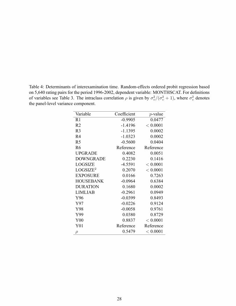
Table 4: Determinants of interexamination time. Random-effects ordered probit regression basedon 5,640 rating pairs for the period 1996-2002, dependent variable: MONTHSCAT. For de�nitionsof variables see Table 3. The intraclass correlation � is given by �2�=(�2� + 1), where �2� denotesthe panel-level variance component.

Variable Coef�cient p-valueR1 -0.9905 0.0477R2 -1.4196 < 0.0001R3 -1.1395 0.0002R4 -1.0323 0.0002R5 -0.5600 0.0404R6 Reference ReferenceUPGRADE 0.4082 0.0051DOWNGRADE 0.2230 0.1416LOGSIZE -4.5591 < 0.0001LOGSIZE2 0.2070 < 0.0001EXPOSURE 0.0166 0.7263HOUSEBANK -0.0964 0.6384DURATION 0.1680 0.0002LIMLIAB -0.2961 0.0949Y96 -0.0399 0.8493Y97 -0.0226 0.9124Y98 -0.0058 0.9761Y99 0.0380 0.8729Y00 0.8837 < 0.0001Y01 Reference Reference� 0.5479 < 0.0001

28

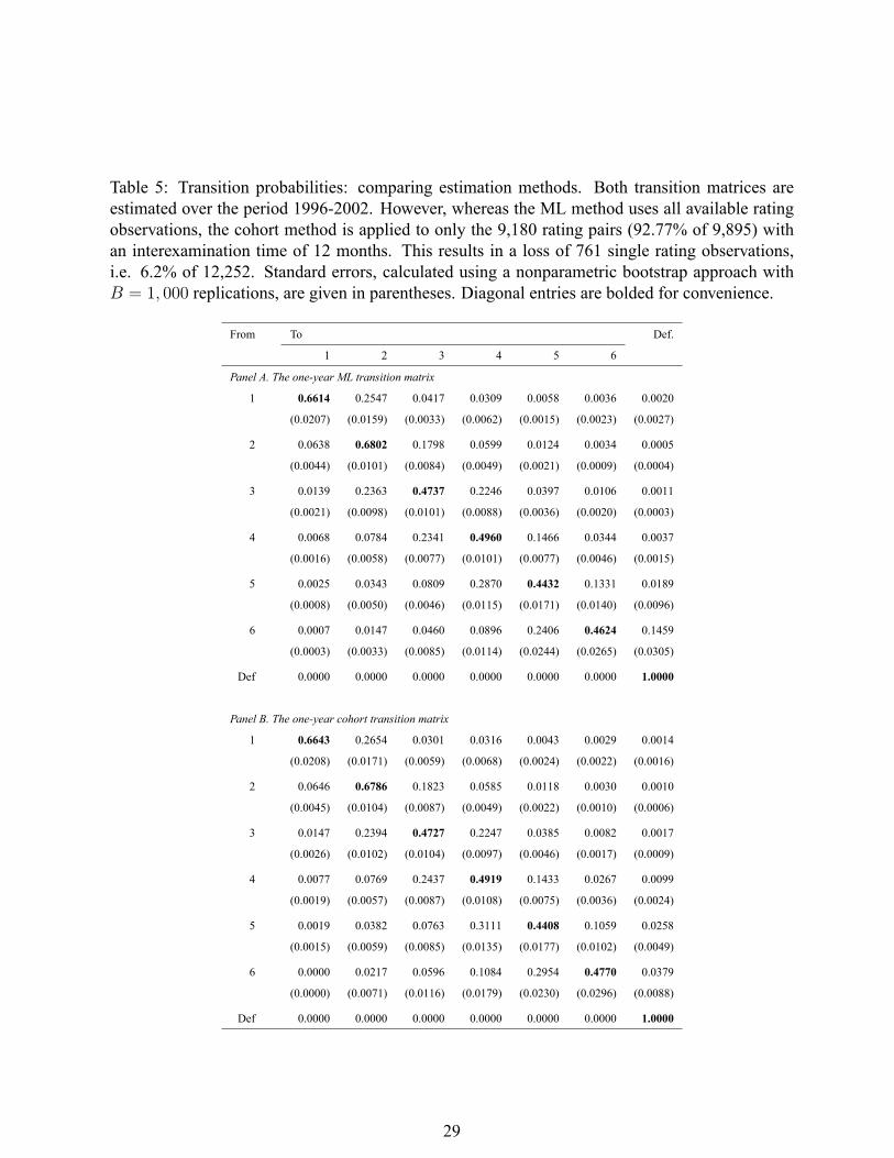
Table 5: Transition probabilities: comparing estimation methods. Both transition matrices areestimated over the period 1996-2002. However, whereas the ML method uses all available ratingobservations, the cohort method is applied to only the 9,180 rating pairs (92.77% of 9,895) withan interexamination time of 12 months. This results in a loss of 761 single rating observations,i.e. 6.2% of 12,252. Standard errors, calculated using a nonparametric bootstrap approach withB = 1; 000 replications, are given in parentheses. Diagonal entries are bolded for convenience.

From To Def.

1 2 3 4 5 6

Panel A. The one-year ML transition matrix

1 0.6614 0.2547 0.0417 0.0309 0.0058 0.0036 0.0020

(0.0207) (0.0159) (0.0033) (0.0062) (0.0015) (0.0023) (0.0027)

2 0.0638 0.6802 0.1798 0.0599 0.0124 0.0034 0.0005

(0.0044) (0.0101) (0.0084) (0.0049) (0.0021) (0.0009) (0.0004)

3 0.0139 0.2363 0.4737 0.2246 0.0397 0.0106 0.0011

(0.0021) (0.0098) (0.0101) (0.0088) (0.0036) (0.0020) (0.0003)

4 0.0068 0.0784 0.2341 0.4960 0.1466 0.0344 0.0037

(0.0016) (0.0058) (0.0077) (0.0101) (0.0077) (0.0046) (0.0015)

5 0.0025 0.0343 0.0809 0.2870 0.4432 0.1331 0.0189

(0.0008) (0.0050) (0.0046) (0.0115) (0.0171) (0.0140) (0.0096)

6 0.0007 0.0147 0.0460 0.0896 0.2406 0.4624 0.1459

(0.0003) (0.0033) (0.0085) (0.0114) (0.0244) (0.0265) (0.0305)

Def 0.0000 0.0000 0.0000 0.0000 0.0000 0.0000 1.0000

Panel B. The one-year cohort transition matrix

1 0.6643 0.2654 0.0301 0.0316 0.0043 0.0029 0.0014

(0.0208) (0.0171) (0.0059) (0.0068) (0.0024) (0.0022) (0.0016)

2 0.0646 0.6786 0.1823 0.0585 0.0118 0.0030 0.0010

(0.0045) (0.0104) (0.0087) (0.0049) (0.0022) (0.0010) (0.0006)

3 0.0147 0.2394 0.4727 0.2247 0.0385 0.0082 0.0017

(0.0026) (0.0102) (0.0104) (0.0097) (0.0046) (0.0017) (0.0009)

4 0.0077 0.0769 0.2437 0.4919 0.1433 0.0267 0.0099

(0.0019) (0.0057) (0.0087) (0.0108) (0.0075) (0.0036) (0.0024)

5 0.0019 0.0382 0.0763 0.3111 0.4408 0.1059 0.0258

(0.0015) (0.0059) (0.0085) (0.0135) (0.0177) (0.0102) (0.0049)

6 0.0000 0.0217 0.0596 0.1084 0.2954 0.4770 0.0379

(0.0000) (0.0071) (0.0116) (0.0179) (0.0230) (0.0296) (0.0088)

Def 0.0000 0.0000 0.0000 0.0000 0.0000 0.0000 1.0000

29

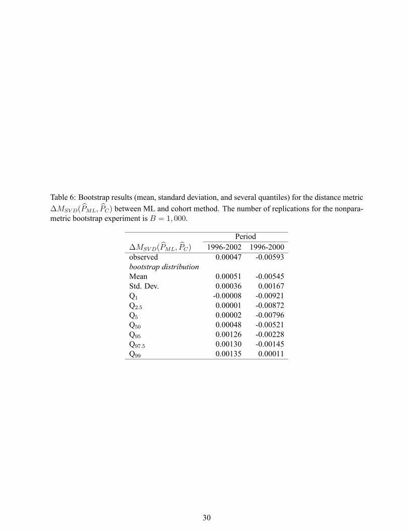
Table 6: Bootstrap results (mean, standard deviation, and several quantiles) for the distance metric�MSV D( bPML; bPC) between ML and cohort method. The number of replications for the nonpara-metric bootstrap experiment is B = 1; 000.

Period�MSV D( bPML; bPC) 1996-2002 1996-2000observed 0.00047 -0.00593bootstrap distributionMean 0.00051 -0.00545Std. Dev. 0.00036 0.00167Q1 -0.00008 -0.00921Q2:5 0.00001 -0.00872Q5 0.00002 -0.00796Q50 0.00048 -0.00521Q95 0.00126 -0.00228Q97:5 0.00130 -0.00145Q99 0.00135 0.00011

30

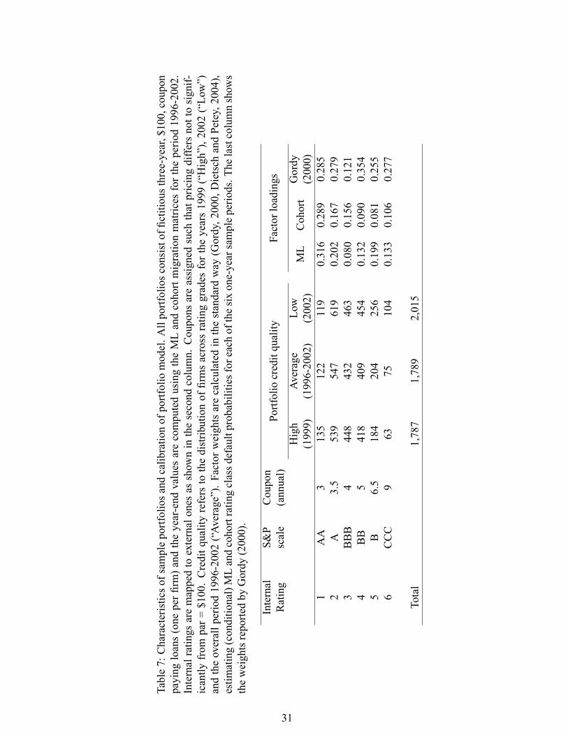
Table7:Characteristicsofsampleportfoliosandcalibrationofportfoliomodel.Allportfoliosconsistof�ctitiousthree-year,$100,coupon

payingloans(oneper�rm)andtheyear-endvaluesarecomputedusingtheMLandcohortmigrationmatricesfortheperiod1996-2002.

Internalratingsaremappedtoexternalonesasshowninthesecondcolumn.Couponsareassignedsuchthatpricingdiffersnottosignif-

icantlyfrom

par=$100.Creditqualityreferstothedistributionof�rmsacrossratinggradesfortheyears1999(�High�),2002(�Low�)

andtheoverallperiod1996-2002(�Average�).Factorweightsarecalculatedinthestandardway(Gordy,2000,DietschandPetey,2004),

estimating(conditional)MLandcohortratingclassdefaultprobabilitiesforeachofthesixone-yearsampleperiods.Thelastcolumnshows

theweightsreportedbyGordy(2000).

Internal

Rating

S&P

scale

Coupon

(annual)

Portfoliocreditquality

Factorloadings

High

(1999)

Average

(1996-2002)

Low

(2002)

ML

Cohort

Gordy

(2000)

1AA

3135

122

119

0.316

0.289

0.285

2A

3.5

539

547

619

0.202

0.167

0.279

3BBB

4448

432

463

0.080

0.156

0.121

4BB

5418

409

454

0.132

0.090

0.354

5B

6.5

184

204

256

0.199

0.081

0.255

6CCC

963

75104

0.133

0.106

0.277

Total

1,787

1,789

2,015

31

Table8:Creditriskcapital:comparingestimationmethods.Creditriskcapitalforaone-yearhorizonascomputedbyaone-factorversion

ofCreditMetricsR .Creditspreadsandtheone-yearforwardzero-couponU.S.TreasuryyieldcurvethatprevailedonJuly19,2005are

takenanda40%recoveryrateisassumed.ThesampleportfoliosandthethreesetsoffactorweightsareasdescribedinTable7.Monte

Carlosimulations(100,000trials)areusedtoobtaintheportfoliovaluedistributionsoneyearhence.

Factorloadings

ML

Cohort

Gordy(2000)

Cohort

ML

%Cohort

ML

Cohort

ML

%Cohort

ML

Cohort

ML

%Cohort

ML

Highqualityportfolio(1999)

Meanhorizonvalue($)

183,389183,085100.17%

183,388183,084100.17%

183,382183,080100.16%

Std.dev.ofvalue($)

634

642

98.75%

484

506

95.65%

1,119

1,100101.73%

VaR(99%)($)

1,834

1,808101.44%

1,331

1,369

97.22%

3,662

3,393107.93%

VaR(99.9%)($)

2,711

2,654102.15%

1,945

1,960

99.23%

6,215

5,489113.23%

Averagequalityportfolio(1996-2002)

Meanhorizonvalue($)

183,747183,351100.22%

183,747183,351100.22%

183,748183,353100.22%

Std.dev.ofvalue($)

666

689

96.66%

497

534

93.07%

1,153

1,169

98.63%

VaR(99%)($)

1,929

1,925100.21%

1,364

1,427

95.59%

3,785

3,599105.17%

VaR(99.9%)($)

2,906

2,835102.50%

1,962

2,046

95.89%

6,236

5,798107.55%

Lowqualityportfolio(2002)

Meanhorizonvalue($)

207,204206,608100.29%

207,203206,607100.29%

207,212206,617100.29%

Std.dev.ofvalue($)

792

841

94.17%

577

639

90.30%

1,363

1,433

95.12%

VaR(99%)($)

2,274

2,330

97.60%

1,573

1,696

92.75%

4,451

4,384101.53%

VaR(99.9%)($)

3,427

3,454

99.22%

2,284

2,383

95.85%

7,287

6,835106.61%

32

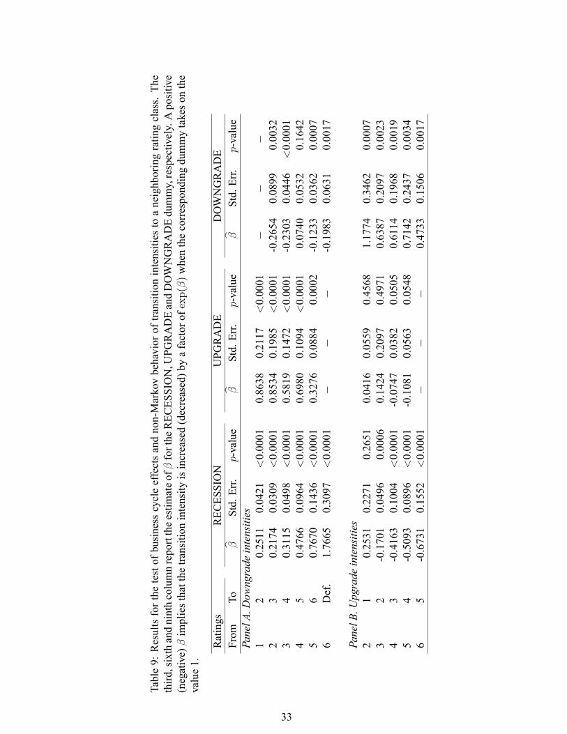
Table9:Resultsforthetestofbusinesscycleeffectsandnon-Markovbehavioroftransitionintensitiestoaneighboringratingclass.The

third,sixthandninthcolumnreporttheestimateof�fortheRECESSION,UPGRADEandDOWNGRADEdummy,respectively.Apositive

(negative)�impliesthatthetransitionintensityisincreased(decreased)byafactorofexp(�)whenthecorrespondingdummytakesonthe

value1.

Ratings

RECESSION

UPGRADE

DOWNGRADE

From

Tob �

Std.Err.

p-value

b �Std.Err.

p-value

b �Std.Err.

p-value

PanelA.Downgradeintensities

12

0.2511

0.0421

<0.0001

0.8638

0.2117

<0.0001

��

�2

30.2174

0.0309

<0.0001

0.8534

0.1985

<0.0001

-0.2654

0.0899

0.0032

34

0.3115

0.0498

<0.0001

0.5819

0.1472

<0.0001

-0.2303

0.0446

<0.0001

45

0.4766

0.0964

<0.0001

0.6980

0.1094

<0.0001

0.0740

0.0532

0.1642

56

0.7670

0.1436

<0.0001

0.3276

0.0884

0.0002

-0.1233

0.0362

0.0007

6Def.

1.7665

0.3097

<0.0001

��

�-0.1983

0.0631

0.0017

PanelB.Upgradeintensities

21

0.2531

0.2271

0.2651

0.0416

0.0559

0.4568

1.1774

0.3462

0.0007

32

-0.1701

0.0496

0.0006

0.1424

0.2097

0.4971

0.6387

0.2097

0.0023

43

-0.4163

0.1004

<0.0001

-0.0747

0.0382

0.0505

0.6114

0.1968

0.0019

54

-0.5093

0.0896

<0.0001

-0.1081

0.0563

0.0548

0.7142

0.2437

0.0034

65

-0.6731

0.1552

<0.0001

��

�0.4733

0.1506

0.0017

33