ESTIMATION OF RARE DESIGN RAINFALLS FOR …€¦ · 2.1.1 BoM and DoE gauge comparison.....6 2.1.2...
127
Surface Water Hydrology Report Series HY17 Estimation of Rare Design Rainfalls for Western Australia Department of Environment i ESTIMATION OF RARE DESIGN RAINFALLS FOR WESTERN AUSTRALIA Application of the CRC-FORGE Method Prepared by Jacqueline Durrant and Sally Bowman Water Resources Division Department of Environment DEPARTMENT OF ENVIRONMENT SURFACE WATER HYDROLOGY REPORT SERIES REPORT NO. HY17 DECEMBER, 2004
-
Upload
truongdung -
Category
Documents
-
view
216 -
download
1
Transcript of ESTIMATION OF RARE DESIGN RAINFALLS FOR …€¦ · 2.1.1 BoM and DoE gauge comparison.....6 2.1.2...
Surface Water Hydrology Report Series HY17 Estimation of Rare Design Rainfalls for Western Australia
Department of Environment i
ESTIMATION OF RARE DESIGN RAINFALLS FORWESTERN AUSTRALIA
Application of the CRC-FORGE Method
Prepared by
Jacqueline Durrant and Sally Bowman
Water Resources Division
Department of Environment
DEPARTMENT OF ENVIRONMENT
SURFACE WATER HYDROLOGY REPORT SERIES
REPORT NO. HY17
DECEMBER, 2004
Estimation of Rare Design Rainfalls for Western Australia Surface Water Hydrology Report Series HY17
ii Department of Environment
Acknowledgments
The WA CRC-FORGE project was funded by the Water Corporation and Main Roads Western Australia. The WADepartment of Environment acknowledges the initial development of the CRC-FORGE method by the CooperativeResearch Centre for Catchment Hydrology (Nandakumar et al, 1997), with changes to the CRC-FORGE method madeby the Department of Environment to reflect Western Australian hydrometeorological conditions. The authors wouldlike to thank staff from Department of the Environment including John Ruprecht and Simon Rodgers for their technicaladvice and Mary-ann Berti for assistance with data processing. The authors also sincerely thank Dr Nanda Nandakumarand Erwin Weinmann for their technical advice and ongoing support for the project, and Dr Nandakumar for thenumerous changes made to the CRC-FORGE programs. In addition, Michelle Dal Pozzo from Bureau of Meteorologyprovided advice with checking the rainfall data and Gary Hargraves from Department of Natural Resources providedadvice and software for assisting in the estimation of areal reduction factors. The authors would also like to thankSimon Rodgers from the Department of Environment and Leanne Pearce on behalf of the Water Corporation for testingof the database.
For more information contact:
Department of EnvironmentWater Investigations and Assessment BranchPO Box 6740East Perth WA 6004
Recommended reference
The recommended reference for this publication is: Durrant, J.M. & Bowman, S. 2004, Estimation of Rare DesignRainfalls for Western Australia: Application of the CRC-FORGE Method, Department of Environment, Government ofWestern Australia, Surface Water Hydrology Report Series Report No. HY17.
We welcome your feedbackA publication feedback form can be found at the back of this publication.
ISBN 1 920947 701
Printed on recycled stock.
December, 2004
Surface Water Hydrology Report Series HY17 Estimation of Rare Design Rainfalls for Western Australia
Department of Environment iii
Contents
Summary ................................................................................................................... 1
1 Introduction ............................................................................................................ 3
1.1 Background and overview of method ......................................................................31.2 Application to Western Australia..............................................................................3
2 Data preparation.................................................................................................... 6
2.1 Daily rainfall data.....................................................................................................62.1.1 BoM and DoE gauge comparison ...............................................................62.1.2 Notable point rainfall events........................................................................6
2.2 Initial data screening ...............................................................................................62.3 Extraction of annual and seasonal maxima.............................................................72.4 Checking of maxima................................................................................................92.5 Final data sets .......................................................................................................11
3 Identification of distributions and homogeneous regions .................................... 13
3.1 Stationarity ............................................................................................................133.2 Probability distribution ...........................................................................................14
3.2.1 L-moment ratio diagrams..........................................................................143.2.2 Probability Plot Correlation Coefficient Test .............................................16
3.3 Homogeneity .........................................................................................................183.3.1 Preliminary regions for Western Australia.................................................18
3.4 Regional probability distribution.............................................................................21
4 Application of the CRC-FORGE method at focal stations ................................... 23
4.1 Spatial dependence model ....................................................................................234.1.1 Spatial dependence for Western Australia................................................244.1.2 Additional work on spatial dependence for Western Australia ..................274.1.3 Final homogeneous regions and distributions for spatial dependence .....29
4.2 Derivation of growth curves at focal stations .........................................................334.2.1 Sensitivity testing for separation between regions, distributions and
seasons ....................................................................................................334.2.2 Final growth curves...................................................................................34
5 Derivation of design point rainfalls....................................................................... 36
5.1 Point rainfall estimates ..........................................................................................365.1.1 Point rainfall adjustment ...........................................................................36
Estimation of Rare Design Rainfalls for Western Australia Surface Water Hydrology Report Series HY17
iv Department of Environment
5.2 Grid rainfall estimates............................................................................................375.2.1 Variation with elevation and Intensity Frequency Duration information.....385.2.2 Grid rainfall adjustment and smoothing ....................................................39
5.3 Annual rainfall estimates .......................................................................................395.4 Final design point rainfalls .....................................................................................405.5 Comparison of CRC-FORGE rainfalls with ARR87 data and at-site estimates .....40
6 CRC-FORGE areal reduction factors .................................................................. 43
6.1 Introduction............................................................................................................436.2 Disaggregation of rainfall data for ARF analysis....................................................436.3 Generation of hypothetical catchments .................................................................446.4 Calculation of ARF values .....................................................................................456.5 Regional variability in ARFs...................................................................................466.6 Seasonal variability in ARFs..................................................................................506.7 Fitting procedure for ARF design curves ...............................................................51
6.7.1 ARF for AEP of 0.50 .................................................................................516.7.2 ARF for AEPs < 0.50 ................................................................................546.7.3 Final ARF design curves...........................................................................56
6.8 Comparison of annual CRC-FORGE and ARR87 ARFs .......................................57
7 WA CRC-FORGE EXTRACT .............................................................................. 58
8 Conclusions and recommendations .................................................................... 59
References and recommended reading .................................................................. 61
Appendices
Appendix A – WA CRC-FORGE programs ............................................................. 63
Appendix B - Revised spatial dependence model results ....................................... 69
Appendix C - Smoothing of preliminary grid point values across duration.............. 78
Appendix D - Comparisons of CRC-FORGE and ARR87 design rainfall estimates79
Appendix E - Sample mean values of areal reduction factors for WA .................... 81
Appendix F - Revised areal reduction factor curves for Western Australia ............. 89
Surface Water Hydrology Report Series HY17 Estimation of Rare Design Rainfalls for Western Australia
Department of Environment v
TablesTable 2.1: Number of stations and record length of processed 1-day data for annual and
seasonal rainfall stations within WA and 100 km into the NT.........................................11Table 2.2: Number of annual rainfall stations in each State ...............................................11Table 3.1: Number and percentage of stations that failed the Mann-Kendall and CUSUM
tests ...............................................................................................................................13Table 4.1: Homogeneous regions for summer and winter rainfalls and associated rainfall
districts...........................................................................................................................30Table 4.2: Homogeneous regions for summer and winter rainfalls and their associated
distributions....................................................................................................................33Table 5.1: Summer adjustment coefficients for consistency across duration .....................36Table 5.2: Winter adjustment coefficients for consistency across duration ........................36Table 5.3: Conversion factors for rainfall data from restricted to unrestricted durations.....37Table 5.4: Comparison between CRC-FORGE and ARR87 design rainfall estimates.......41Table 5.5: Comparison between CRC-FORGE and ARR87 approaches...........................41Table 6.1: Number of hypothetical catchments and mean ARFs for annual, summer and
winter initial regions for 24 hour duration, 0.5 AEP and a 250 km2 area ........................47
FiguresFigure 1.1: Western Australian and Northern Territory rainfall districts, major regions and
dominant large scale meteorological processes ..............................................................4Figure 1.2: Flow chart showing application of the CRC-FORGE methodology to Western
Australia...........................................................................................................................5Figure 2.1: Location of Bureau of Meteorology and Department of Environment rainfall
stations for Western Australia and Northern Territory ......................................................7Figure 2.2: Schematic of Daymaxsn display for accumulated data (modified from SKM
2000)................................................................................................................................8Figure 2.3: Schematic of Daymaxsn display for missing data (modified from SKM 2000) ...8Figure 2.4: Maxploti output for rainfall station 004006 for annual.......................................10Figure 2.5: Maxploti output for rainfall station 012008 for winter........................................10Figure 2.6: Stations with greater than 60 years of 1-day annual rainfall data for WA and NT
rainfall districts ...............................................................................................................12Figure 3.1: Annual 1-day maximum data for rainfall station 003009 ..................................13Figure 3.2: Daily rainfall data for rainfall station 003009 ....................................................14Figure 3.3: L-kurtosis versus L-skewness for 1-day annual maxima with greater than 60
years of rainfall ..............................................................................................................15Figure 3.4: L-kurtosis versus L-skewness for 1-day summer maxima with greater than 60
years of rainfall ..............................................................................................................16Figure 3.5: L-kurtosis versus L-skewness for 1-day winter maxima with greater than 60
years of rainfall ..............................................................................................................16Figure 3.6: Location of rainfall stations that did not satisfy a GEV distribution using the
PPCC test (1-day duration for annual, summer and winter with greater than 60 years ofdata)...............................................................................................................................17
Figure 3.7: Regional L-moment diagram (summer, 1-day, greater than 60 years of data).19Figure 3.8: Regional L-moment diagram (winter, 1-day, greater than 60 years of data) ....20Figure 3.9: Regional L-moment diagram (annual, 1-day, greater than 60 years of data)...20
Estimation of Rare Design Rainfalls for Western Australia Surface Water Hydrology Report Series HY17
vi Department of Environment
Figure 3.10: Example of regional L-Moment diagram of L-kurtosis vs L-skewness and thelocations of the stations for the Gascoyne region ..........................................................22
Figure 4.1: Regional maximum and regional average curves diverging (variable spatialdependence model) .......................................................................................................23
Figure 4.2: Variable spatial dependence model for Victoria derived from generated rainfalldata (Nandakumar et al. 1997). .....................................................................................24
Figure 4.3: Spatial dependence model for winter 1-day for the Mid-Pilbara region with GEVdistribution (horizontal lines represent constant Ne model, curves represent variable Ne
model)............................................................................................................................26Figure 4.4: Example of converging regional maximum and regional average curve ..........26Figure 4.5 Example of regional L-Moment diagram of L-Kurtosis vs L-Skewness and the
locations of the stations for the Mid-Pilbara region with one distribution........................28Figure 4.6: Example of regional L-Moment diagram of L-Kurtosis vs L-Skewness and the
locations of the stations for the Mid-Pilbara region with two distributions ......................28Figure 4.7: Revised spatial dependence model for 1-day for the Mid-Pilbara region with
GEV and PE3 distribution ..............................................................................................29Figure 4.8: Spatial dependence models for proposed summer regions for N=200 and
correlation coefficient = 0.2............................................................................................30Figure 4.9: Final summer homogeneous regions...............................................................31Figure 4.10: Final winter homogeneous regions ................................................................32Figure 4.11: Summer and winter growth curves for focal station 008061...........................34Figure 4.12: Summer growth curve for focal station 009534..............................................35Figure 5.1: Sample relationship between index variable and elevation..............................38Figure 5.2: Calculation of annual design rainfalls from seasonal frequency curves ...........40Figure 6.1: Distribution of centroids of annual hypothetical catchments for 250 km2 area .45Figure 6.2: Comparison of annual ARF regions for 24 hour duration and 0.5 AEP............48Figure 6.3: Comparison of winter ARF regions for 24 hour duration and 0.5 AEP .............48Figure 6.4: Comparison of summer ARF regions for 24 hour duration and 0.5 AEP..........49Figure 6.5: Summer areal reduction factor regions (demarcation of South-west region with
greater than 700 mm mean annual rainfall) ...................................................................50Figure 6.6: Comparison of annual, summer and winter ARFs for 24 hour duration and 0.5
AEP................................................................................................................................51Figure 6.7: Annual areal reduction factor curves for AEP of 0.5 ........................................52Figure 6.8: Summer South-west region areal reduction factor curves for AEP of 0.5 ........53Figure 6.9: Summer Rest of State areal reduction factor curves for AEP of 0.5 ................53Figure 6.10: Winter areal reduction factor curves for AEP of 0.5 .......................................54Figure 6.11: Variation of annual ARF with AEP for 1000 km2 catchment area...................55Figure 6.12: Variation of summer (South-west region) ARF with AEP for 1000 km2
catchment area ..............................................................................................................55Figure 6.13: Variation of summer (Rest of State) ARF with AEP for 1000 km2 catchment
area................................................................................................................................56Figure 6.14: Variation of winter ARF with AEP for 1000 km2 catchment area....................56Figure 6.15: Comparison of CRC-FORGE and ARR87 ARFs............................................57
Surface Water Hydrology Report Series HY17 Estimation of Rare Design Rainfalls for Western Australia
Department of Environment 1
Summary
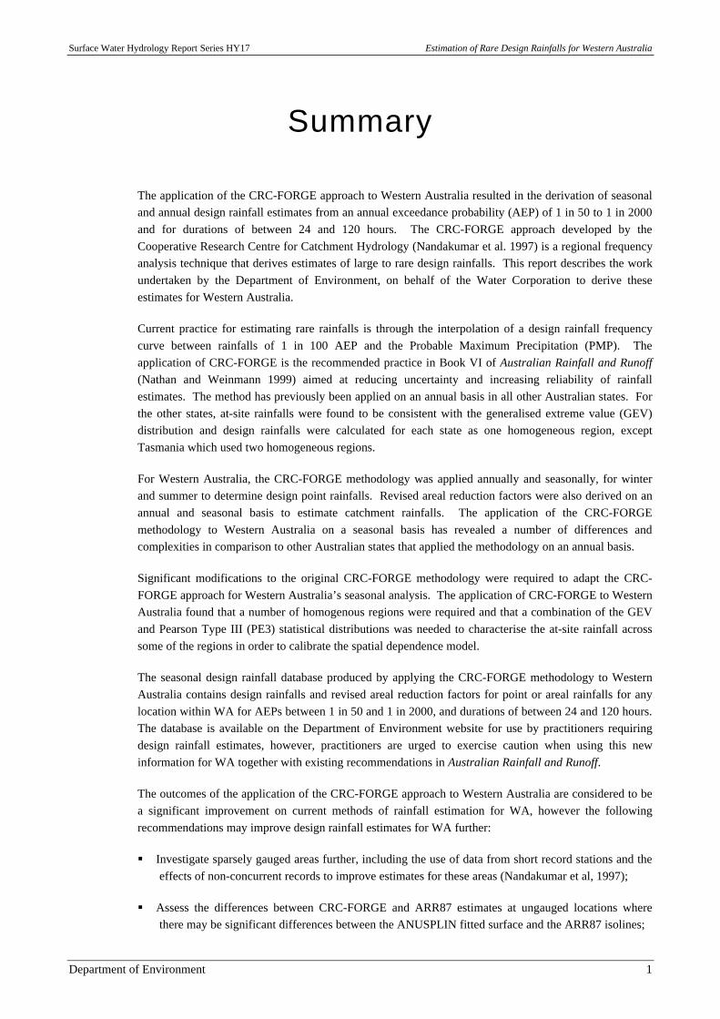
The application of the CRC-FORGE approach to Western Australia resulted in the derivation of seasonaland annual design rainfall estimates from an annual exceedance probability (AEP) of 1 in 50 to 1 in 2000and for durations of between 24 and 120 hours. The CRC-FORGE approach developed by theCooperative Research Centre for Catchment Hydrology (Nandakumar et al. 1997) is a regional frequencyanalysis technique that derives estimates of large to rare design rainfalls. This report describes the workundertaken by the Department of Environment, on behalf of the Water Corporation to derive theseestimates for Western Australia.
Current practice for estimating rare rainfalls is through the interpolation of a design rainfall frequencycurve between rainfalls of 1 in 100 AEP and the Probable Maximum Precipitation (PMP). Theapplication of CRC-FORGE is the recommended practice in Book VI of Australian Rainfall and Runoff(Nathan and Weinmann 1999) aimed at reducing uncertainty and increasing reliability of rainfallestimates. The method has previously been applied on an annual basis in all other Australian states. Forthe other states, at-site rainfalls were found to be consistent with the generalised extreme value (GEV)distribution and design rainfalls were calculated for each state as one homogeneous region, exceptTasmania which used two homogeneous regions.
For Western Australia, the CRC-FORGE methodology was applied annually and seasonally, for winterand summer to determine design point rainfalls. Revised areal reduction factors were also derived on anannual and seasonal basis to estimate catchment rainfalls. The application of the CRC-FORGEmethodology to Western Australia on a seasonal basis has revealed a number of differences andcomplexities in comparison to other Australian states that applied the methodology on an annual basis.
Significant modifications to the original CRC-FORGE methodology were required to adapt the CRC-FORGE approach for Western Australia’s seasonal analysis. The application of CRC-FORGE to WesternAustralia found that a number of homogenous regions were required and that a combination of the GEVand Pearson Type III (PE3) statistical distributions was needed to characterise the at-site rainfall acrosssome of the regions in order to calibrate the spatial dependence model.
The seasonal design rainfall database produced by applying the CRC-FORGE methodology to WesternAustralia contains design rainfalls and revised areal reduction factors for point or areal rainfalls for anylocation within WA for AEPs between 1 in 50 and 1 in 2000, and durations of between 24 and 120 hours.The database is available on the Department of Environment website for use by practitioners requiringdesign rainfall estimates, however, practitioners are urged to exercise caution when using this newinformation for WA together with existing recommendations in Australian Rainfall and Runoff.
The outcomes of the application of the CRC-FORGE approach to Western Australia are considered to bea significant improvement on current methods of rainfall estimation for WA, however the followingrecommendations may improve design rainfall estimates for WA further:
§ Investigate sparsely gauged areas further, including the use of data from short record stations and theeffects of non-concurrent records to improve estimates for these areas (Nandakumar et al, 1997);
§ Assess the differences between CRC-FORGE and ARR87 estimates at ungauged locations wherethere may be significant differences between the ANUSPLIN fitted surface and the ARR87 isolines;

Estimation of Rare Design Rainfalls for Western Australia Surface Water Hydrology Report Series HY17
2 Department of Environment
§ Derive CRC-FORGE design rainfall estimates for durations shorter than 24 hours;
§ Derive areal reduction factors for durations shorter than 24 hours; and
§ Develop CRC-FORGE temporal patterns for design events in the large to rare range.
Surface Water Hydrology Report Series HY17 Estimation of Rare Design Rainfalls for Western Australia
Department of Environment 3
1 Introduction
1.1 Background and overview of method
The CRC-FORGE method is based on the FORGE (FOcussed Rainfall Growth Estimation) conceptdeveloped by the UK Institute of Hydrology (Dales and Reed, 1989). It is a regional frequency analysismethod for estimating Large to Rare rainfalls, defined in Book VI of Australian Rainfall and Runoff(Nathan and Weinmann 1999) as rainfalls ranging between an annual exceedance probability (AEP) of 1in 50 to the credible limit of extrapolation.
Regional methods, including CRC-FORGE, are based on the concept that additional information can begained by pooling standardised data from a number of rainfall sites at a regional scale. The data isstandardised by dividing it by the mean annual or seasonal maxima for a specific duration. Theunderlying assumption is that, after allowing for differences in the annual or seasonal mean of rainfallextremes, the statistical properties of extreme rainfall at different sites in a region are similar, allowingdata from sites with records of limited temporal extent to be combined into a larger spatial sample thatsatisfies basic homogeneity assumptions. This pooling of regional data raises the question as to howmuch information is gained by combining the rainfall records, allowing for the effects of inter-sitecorrelation, or spatial dependence. The CRC-FORGE method resolves this by computing a spatialdependence model which reflects the effective number of independent stations (Ne) in a region. Growthcurves (frequency curves of standardised regional data) of design rainfalls are then generated by plottingthe at-site data and pooling additional data from rainfall sites within areas of increasing size (calledFORGE regions) to estimate rainfalls with decreasing AEPs. The spatial dependence model is used todetermine the plotting position of the data points (Nandakumar et al. 2000). The CRC-FORGEmethodology is outlined in detail in Nandakumar et al. (1997) and Weinmann et al (1999).
1.2 Application to Western Australia
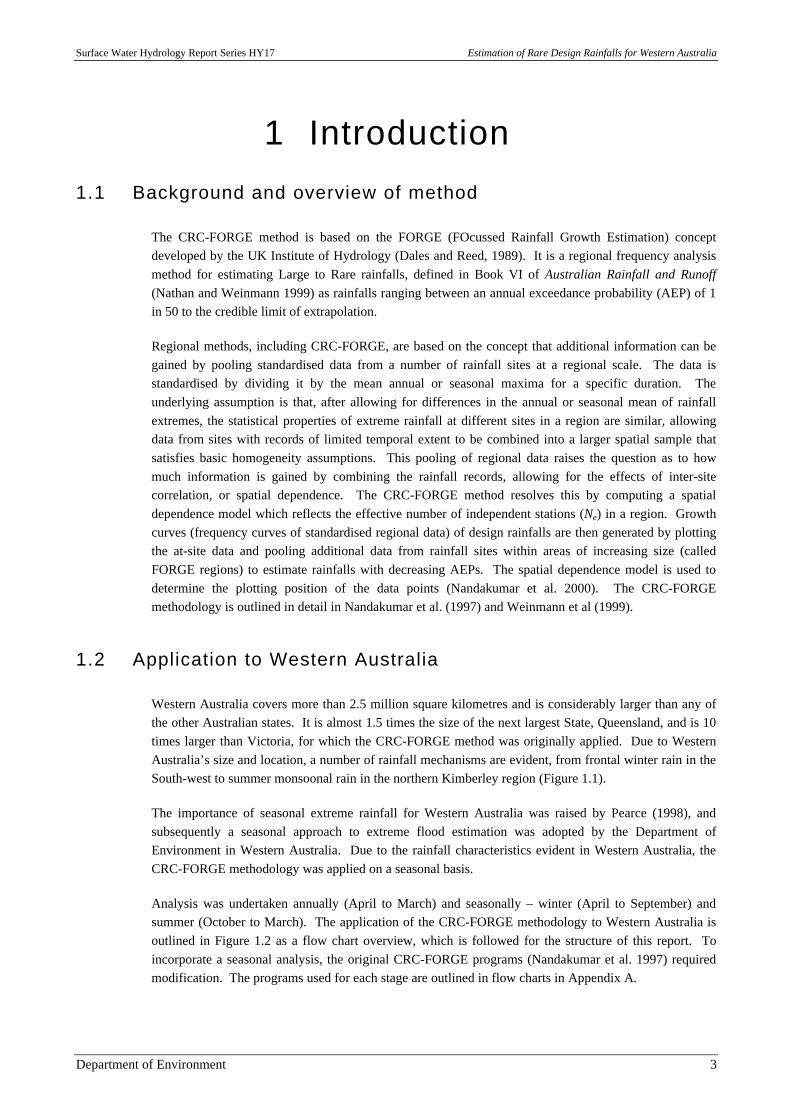
Western Australia covers more than 2.5 million square kilometres and is considerably larger than any ofthe other Australian states. It is almost 1.5 times the size of the next largest State, Queensland, and is 10times larger than Victoria, for which the CRC-FORGE method was originally applied. Due to WesternAustralia’s size and location, a number of rainfall mechanisms are evident, from frontal winter rain in theSouth-west to summer monsoonal rain in the northern Kimberley region (Figure 1.1).
The importance of seasonal extreme rainfall for Western Australia was raised by Pearce (1998), andsubsequently a seasonal approach to extreme flood estimation was adopted by the Department ofEnvironment in Western Australia. Due to the rainfall characteristics evident in Western Australia, theCRC-FORGE methodology was applied on a seasonal basis.
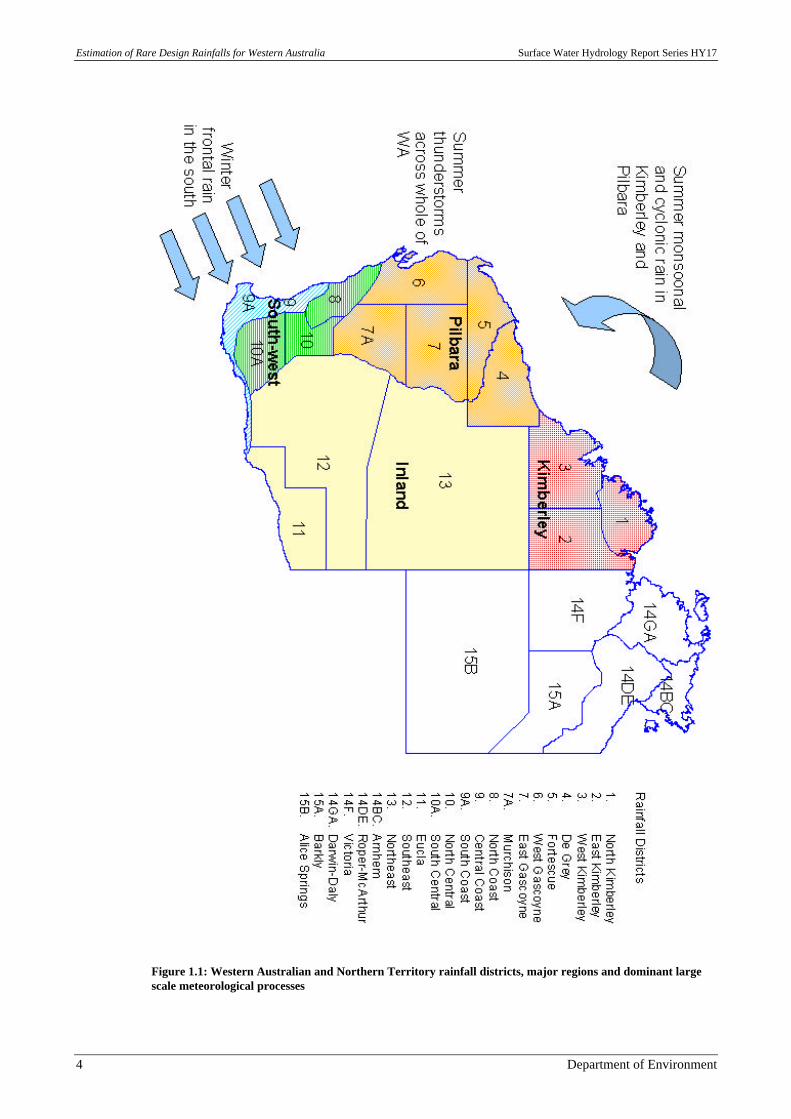
Analysis was undertaken annually (April to March) and seasonally – winter (April to September) andsummer (October to March). The application of the CRC-FORGE methodology to Western Australia isoutlined in Figure 1.2 as a flow chart overview, which is followed for the structure of this report. Toincorporate a seasonal analysis, the original CRC-FORGE programs (Nandakumar et al. 1997) requiredmodification. The programs used for each stage are outlined in flow charts in Appendix A.
Estimation of Rare Design Rainfalls for Western Australia Surface Water Hydrology Report Series HY17
4 Department of Environment
Figure 1.1: Western Australian and Northern Territory rainfall districts, major regions and dominant largescale meteorological processes
Surface Water Hydrology Report Series HY17 Estimation of Rare Design Rainfalls for Western Australia
Department of Environment 5
Assemble and checkdaily rainfall data
Extract maximum series forAnnual, Summer and Winter
Select probabilitydistribution
Determinehomogeneous regions
Derive spatialdependence model
Derive growth curvesat focus stations
Gridded values ofrainfalls
Preliminary pointrainfalls
New point rainfalls
Disaggregate rainfalldata
Select hypotheticalcatchments
Calculate arealreduction factors
Fit equation to meanvalues
New areal reductionfactors
New Design Rainfalls for Western AustraliaAEP 1-in-50 to 1-in-2000Duration 24 – 120 hours
CRC-FORGE Areal Reduction Factors
Figure 1.2: Flow chart showing application of the CRC-FORGE methodology to Western Australia
Estimation of Rare Design Rainfalls for Western Australia Surface Water Hydrology Report Series HY17
6 Department of Environment
2 Data preparation
2.1 Daily rainfall data
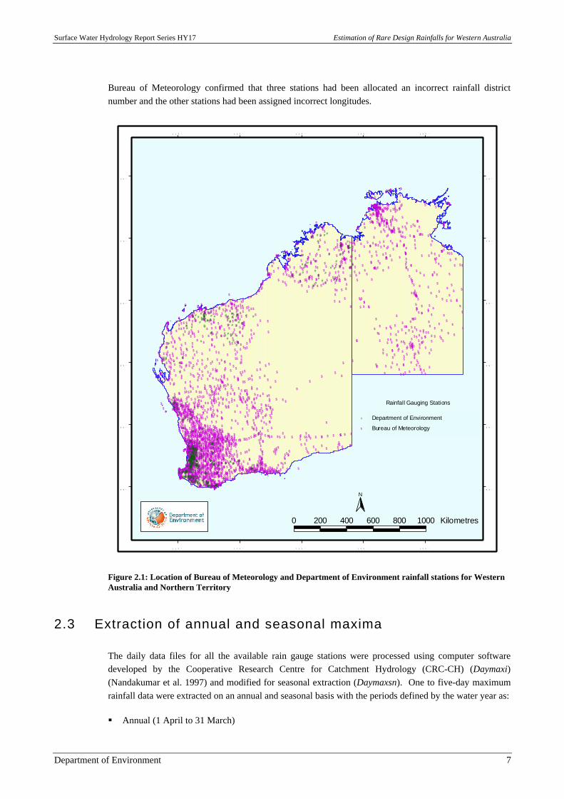
Preparation of a rainfall data set was required for the application of the CRC-FORGE method to WesternAustralia (WA). This involved the processing of the complete data set of Western Australia’s Bureau ofMeteorology (BoM) daily rainfall stations and the Department of Environment (DoE) pluviographstations with 3171 stations in total. Additional Bureau of Meteorology rainfall stations (650) from theNorthern Territory (NT) were also processed to avoid “edge effects”. In total, 3821 rainfall stations(Figure 2.1) were processed. Once the data was processed, only rainfall stations that fell within a 100 kmband adjacent to the WA border were selected from the NT to allow coverage of the Ord Catchment,which extends from the Northern Territory into the Kimberley region of WA. Stations in South Australiathat were adjacent to the Western Australian border were not included as only three stations fell within100 km of the border along the Eyre Highway and the inclusion of these stations resulted in minimalchanges in avoiding any “edge effects”.
The Bureau of Meteorology and Department of Environment rainfall records used in the analysis rangefrom the period 1906 to 2002 and 1966 to 2002 respectively, although most of the stations have a recordlength of only part of these periods.
2.1.1 BoM and DoE gauge comparison
The Bureau of Meteorology and Department of Environment rainfall gauges operate on different setupmethods. A Bureau of Meteorology gauge is typically at ground level with the orifice 300 mm above this(Bureau of Meteorology 1997) whereas the Department of Environment set the entire gauge raised onemetre above the ground level (Davies and Chapman 1997). The reliability of the two different gaugeswas assessed by comparing double mass curves between closely located Bureau of Meteorology andDepartment of Environment stations. The data was found to be comparable and therefore the data fromboth sets of gauges were used in the analysis.
2.1.2 Notable point rainfall events
Notable point rainfall events from other sources as listed in the Bureau of Meteorology’s supplement toBulletin 53 (1996) were investigated. These events were found to be already included in the datacollected. The availability and usefulness of data from private sources such as mining companies wasalso investigated. The majority of this data was already registered in the Bureau of Meteorology systemand those that were not listed did not operate over a sufficient record length or did not add any extrainformation to the data set.
2.2 Initial data screening
The raw data set was evaluated to identify stations with incorrectly assigned latitudes and longitudes.This was undertaken by plotting the stations grouped by their assigned rainfall districts, then overlaying aGIS layer of the district boundaries. The Bureau of Meteorology was approached to confirm the locationand the assigned rainfall district for 14 stations that plotted outside their respective rainfall districts. The
Surface Water Hydrology Report Series HY17 Estimation of Rare Design Rainfalls for Western Australia
Department of Environment 7
Bureau of Meteorology confirmed that three stations had been allocated an incorrect rainfall districtnumber and the other stations had been assigned incorrect longitudes.
$$
$$
$
$
$
$$
$$$
$$$
$
$$$$
$$
$$$
$
$
$
$
$
$
$
$
$
$
$$$$$$$$$$$$
$
$$$$
$
$
$
$
$
$$$
$
$$
$$
$$$
$
$
$
$
$
$$
$
$
$
$
$$
$
$
$
$
$$
$
$
$
$$
$$$
$$$
$
$$
$
$$$
$$
$$$
$$$$$$$$$$$
$ $$$$$
$$$$$$$$$
$$$$$$$$$$$$$$$$$
$$$$$$$$$$
$$$
$ $$$$$$$$$$$$$$ $$$$$ $$$$
$$$$$$
$ $$$$$
$$$$$$$$$
$
$$
$$$
$$$$
$
$
$$$$
$$$$
$$
$$
$$
$$
$
$$
$
$
$
$
$$$
$$
$$
$
$
$$$
$
$$ $
$
$$
$$$
$$
$$
$
$
$$$
$
$
$
$
$$ $$
$
$$
$$
$
$
$$
$
$
$
$
$$$
$
$$
$
$$$
$
$
$$
$
$
$$
$
$$$$
$
$$
$$$$$
$
$$
$$
$
$$
$
$$$$$$$$$$$$$$$$$$$$$$$$$$$$$
$$$$$$$$$$
$
$
$$$$$$$$$$$$$$$$$$$$$$$$$
$$$$$$$
$$$$
$$$$$$
$
$$$
$
$
$$
$
$
$$ $$
$
$$$
$ $$$$
$
$$$
$$
$$$$$
$
$
$$$$
$$$$
$
$
$ $
$$$$$
$
$$
$
$$
$$$$
$
$
$
$
$ $$
$
$
$
$
$
$
$
$$
$
$
$
$$$
$
$$
$$ $$
$
$
$$
$$
$
$
$
$$
$$
$
$
$
$
$$
$$
$
$
$
$
$
$$
$ $
$
$$
$
$
$
$$$
$
$
$
$
$
$
$
$$
$
$
$$
$
$$
$
$
$
$$
$
$
$
$$
$
$
$
$
$
$
$
$
$
$
$
$
$$
$$
$
$
$
$
$
$
$$
$$$
$
$
$
$
$
$ $ $
$ $
$
$
$
$
$$
$
$$
$
$
$
$
$
$
$$
$
$
$
$
$$
$
$
$
$$$
$
$
$
$
$$
$
$ $$
$
$$
$
$
$
$
$
$$
$
$
$
$ $$
$$$$
$$$
$
$
$$
$
$$
$
$
$
$
$
$
$
$
$
$ $
$$ $
$
$
$$$
$
$$ $
$
$ $
$$$ $
$
$
$$
$
$$
$
$
$$
$$
$$
$$
$
$
$
$$
$$$
$ $
$
$
$ $$
$$
$
$
$
$
$
$
$
$
$
$
$$
$
$
$$$
$
$
$
$$$
$
$$
$$$$
$ $$
$
$$
$
$
$
$$
$
$
$
$
$
$$
$ $
$
$
$
$$
$
$
$$
$
$$$$
$
$$
$
$
$$$
$
$
$
$$
$ $
$
$
$$
$
$
$
$$
$
$ $
$$
$$$
$$
$
$
$
$
$
$
$ $
$
$
$
$
$
$$$
$
$
$
$
$
$$$
$
$
$$
$
$$
$
$
$
$
$$
$
$
$
$
$$$
$
$
$
$
$
$
$
$$
$
$
$
$
$
$
$
$
$
$
$
$$
$
$
$
$
$
$
$
$
$
$
$
$
$$$
$
$
$
$
$
$
$$
$
$
$
$
$
$
$
$
$
$$
$$
$
$
$$
$
$
$
$
$
$
$ $$
$
$
$
$
$ $
$$
$
$
$
$$
$
$
$
$
$
$$
$
$
$
$
$
$$
$
$
$
$
$
$$
$
$$
$
$
$
$$
$
$$$
$
$
$
$
$
$$
$
$
$
$
$
$
$
$
$
$
$
$
$
$
$
$
$$
$
$
$
$
$$
$
$
$
$ $
$
$
$
$
$
$
$$
$
$
$
$
$
$
$
$
$
$
$
$
$$
$
$
$
$
$
$
$
$
$
$$
$
$
$$
$
$
$
$
$
$
$$ $
$
$
$
$
$
$
$
$
$
$
$
$
$
$
$
$
$
$
$$
$
$
$
$
$
$
$
$$$
$
$
$
$
$$
$
$
$
$
$
$
$
$
$
$$
$
$
$$
$
$
$
$
$
$
$$ $$
$
$ $ $
$
$
$$
$
$$
$
$
$$
$
$$
$
$
$
$
$$
$
$
$
$
$
$
$
$
$$ $
$$
$
$
$
$
$
$
$
$
$
$$ $
$$
$
$
$
$
$ $
$
$
$
$
$
$
$
$$
$
$
$$
$$
$ $
$$$$$
$
$
$
$
$
$
$$$
$$
$$
$
$
$$
$$$
$
$$
$
$
$
$$
$
$
$$
$
$
$
$
$$
$$
$$
$
$
$$
$$
$
$
$
$
$$
$
$
$
$
$
$
$$
$ $
$$
$$$$
$
$$
$
$$
$
$$
$
$ $
$
$
$
$
$ $$
$
$
$
$$
$$
$$
$
$
$
$
$ $
$
$$
$
$
$
$$$
$$
$
$$
$$
$
$
$$
$
$
$
$
$
$
$
$$
$
$
$
$
$
$
$
$$
$
$
$
$
$
$$
$
$$
$
$
$
$
$
$
$
$
$
$
$
$
$
$ $
$$
$
$
$
$ $
$
$
$
$
$
$
$$
$
$$
$
$
$
$
$
$
$$
$$$
$
$
$
$
$
$
$ $$ $
$
$
$
$
$
$ $
$$
$
$ $$
$
$$
$$
$
$$
$
$
$$
$
$$
$$
$$
$ $
$
$
$
$
$
$$
$
$
$
$
$
$
$$
$
$
$
$
$
$
$$
$ $
$
$$$$
$
$
$ $
$$
$$
$
$
$
$$
$$$
$
$
$
$
$
$$$
$
$
$$$
$
$$
$ $$$$$
$
$
$$$
$
$$
$$$
$
$
$
$$
$$$$
$
$
$$
$$$$$$$
$
$
$
$$$
$
$$
$
$$
$
$
$
$
$$$$
$$
$
$$
$
$$$
$
$
$$$$$$$
$
$ $$$$$ $$
$
$
$
$
$
$
$
$
$
$$
$$$$$$$
$
$
$$
$
$$
$$$$$
$$ $
$
$
$$
$
$$$$
$
$$$
$
$
$$
$$
$
$
$
$
$
$
$
$
$$$$$
$$
$$
$
$$$
$$$$$$
$$$$$$
$
$
$ $
$
$$
$$$
$
$$
$$
$
$
$$$$ $$
$$
$$$$
$$$
$
$$
$
$$
$
$
$$$
$
$$$$
$
$
$
$
$
$$$
$
$
$$$$ $$
$
$
$$
$$
$
$
$
$
$
$
$
$$$$
$
$
$
$$
$
$$
$
$
$
$
$
$
$$
$$
$
$
$
$
$
$ $$
$ $
$
$$
$
$$
$
$
$$
$$ $
$$
$$
$
$ $
$$
$
$
$
$$
$
$$
$
$
$$
$
$
$$
$ $$$ $
$
$$ $$$ $$
$
$
$
$
$
$
$
$
$
$$$
$
$
$
$$
$
$
$
$$$
$$
$
$
$
$
$
$$
$$
$
$$
$
$
$
$
$
$
$
$$
$$
$$$
$
$$$
$$
$$
$
$
$
$
$
$$
$$
$$
$
$
$$
$
$$
$
$ $$
$
$
$
$$ $
$
$
$
$
$$
$
$$$
$$$
$$$$
$
$$
$
$
$
$
$
$
$
$
$$
$
$ $
$
$ $
$$
$
$ $
$
$$$$
$
$
$$$$
$$ $
$$
$
$
$$
$
$$
$
$
$$
$$
$
$
$$
$
$
$
$
$
$
$ $
$
$
$
$$
$
$$
$
$
$
$
$
$$
$$
$$$
$$
$
$
$$
$
$$
$$ $
$
$
$$
$
$
$
$
$$$
$ $$ $$ $$ $$ $$$
$
$$
$$
$
$
$
$$
$$
$
$
$
$
$
$ $
$
$
$$$
$
$$$
$
$$
$$
$$$
$
$ $$
$
$
$
$
$$
$
$
$
$
$$$ $$$
$
$
$
$
$$$$
$$
$
$
$
$$$$$$$$$$$
$$$$$
$$
$$$
$
$
$$$
$
$
$
$
$ $$$
$
$
$
$
$
$$
$ $
$
$
$
$
$$$
$
$$
$$
$$$
$
$$
$
$
$$$
$
$
$
$$
$
$$$
$
$
$$
$ $
$
$
$
$
$
$$
$
$$
$
$
$
$$
$
$
$$
$$
$
$
$
$
$$$
$
$
$$$
$
$$
$$$ $
$$
$$
$
$
$$$
$
$
$
$
$$
$$
$
$
$ $
$
$$$$
$
$
$
$
$$
$$
$$$
$
$
$$
$$
$
$$
$
$ $
$$$
$
$
$$
$$ $
$$
$$
$
$
$
$
$$$
$
$
$
$$
$
$$$
$$ $
$$
$
$$
$$
$
$
$$$
$$
$
$$
$
$
$
$$
$$$ $$
$$
$$ $
$
$
$$
$ $$
$$
$
$
$
$
$
$
$
$$
$
$ $
$
$$
$
$
$$
$$
$$$
$
$
$
$
$
$ $
$$
$
$$
$$
$ $
$
$
$
$$$
$ $$
$$$$
$
$$ $
$
$$$$
$
$
$
$$
$
$$ $
$
$$ $
$$$$
$$ $
$ $
$
$
$
$
$
$
$ $
$
$
$
$
$
$
$
$
$
$$
$$
$
$
$
$
$
$
$$
$ $$ $
$$
$
$$
$$
$
$
$$$
$$ $
$$
$$$ $
$$
$
$
$
$
$
$
$
$
$$
$
$$$ $
$
$
$
$
$
$
$
$
$$
$
$
$$$
$$
$$
$
$
$
$
$
$
$
$
$
$$ $$
$$
$$
$
$$ $
$
$ $
$ $$
$$
$
$$$
$
$
$
$
$$ $$$
$ $
$
$
$$$
$$
$$
$
$$ $$
$$
$
$ $
$
$
$$
$
$ $$
$
$ $$
$
$$
$
$ $$$
$
$
$$
$$
$
$
$
$
$
$ $
$
$
$
$ $
$
$
$
$
$
$
$$
$
$
$
$
$
$ $$
$$
$
$
$
$
$
$
$
$$$
$
$
$
$
$
$
$
$ $
$
$$
$$ $$$
$
$$
$
$
$$
$$ $
$$
$
$
$
$
$$
$
$
$
$
$
$
$$
$$
$
$
$
$$
$
$
$
$ $
$
$$
$
$
$
$
$
$
$
$
$
$
$
$
$
$ $
$
$ $
$
$
$$
$$$
$
$$ $ $$
$$
$
$
$
$
$$$
$
$
$$
$$
$$
$$$
$
$$
$
$
$
$$
$
$ $
$
$
$
$
$
$
$ $
$
$
$
$
$
$$ $$
$
$$
$
$ $
$
$ $
$$
$ $ $$
$
$
$
$
$
$
$
$ $
$
$
$$
$
$
$
$
$$
$
$
$$
$$
$
$
$
$
$
$
$
$
$
$$
$
$
$
$$
$
$
$$
$
$
$$$
$
$$$
$
$
$$
$
$
$
$
$ $
$
$
$
$
$
$$
$
$$$
$ $
$
$
$$
$
$ $
$
$
$
$
$
$$
$$
$
$$$ $
$
$$$
$$$$
$
$
$
$
$$
$
$
$
$
$$$
$
$$$$
$
$
$
$
$
$$
$
$
$
$
$
$
$
$$
$
$
$
$
$
$
$$
$
$
$$
$
$
$ $$ $$
$$
$ $
$$
$
$
$
$
$
$
$
$
$
$
$
$
$
$
$
$
$$$
$
$
$
$
$$
$
$$
$
$$
$$$$$
$$
$$
$
$$
$
$
$
$
$$$
$
$
$
$
$$
$$
$
$
$
$$
$
$
$
$ $$
$$
$
$
$$
$$$$$
$
$$
$
$
$
$
$
$
$
$
$$
$
$
$
$
$
$
$
$$
$
$$
$
$
$
$
$
$
$
$
$
$
$
$
$
$
$
$$
$
$
$$
$
$
$
$
$
$
$
$
$
$$
$
$
$
$$
$$
$
$
$
$
$
$
$
$
$
$
$
$$
$ $
$$
$$
$
$
$$$
$$$
$
$
$$$ $ $
$
$$$
$
$
$
$
$
$$$
$
$
$
$$ $
$
$
$
$$
$
$
$
$$$
$
$
$
$
$
$
$
$ $
$
$
$
$
$
$
$$
$
$$
$
$
$
$$$
$
$
$
$ $
$
$
$
$$
$
$$
$
$
$
$
$
$
$
$
$
$ $
$
$
$$$
$
$$
$
$
$
$
$
$
$
$
$
$$
$$
$
$$
$
$
$
$
$
$
$
$
$
$
$$
$
$ $$
$
$$$
$
$
$
$ $$
$
$$
$
$
$
$
$
$
$
$
$$
$
$$
$
$ $
$$
$
$
$
$
$
$$
$
$
$
$ $
$
$
$
$
$
$$
$
$
$
$
$
$
$
$
$$
$
$
$
$
$$
$
$
$
$$$$$$
$$
$
$$
$$
$$
$$
$
$$$
$
$
$
$$ $$$
$
$
$$
$
$$$
$
$
$
$
$
$$$
$
$
$
$
$
$$$
$
$$ $$
$
$
$
$
$
$$$$
$$
$
$
$$
$
$
$$$$$ $$$
$
$$$$
$$
$ $
$$$
$
$
$
$$
$
$$
$$
$
$
$
$ $$ $
$
$$
$$$$
$$$
$$$ $$
$$$
$
$$$
$
$
$
$$
$
$
$
$
$$
$
$
$$
$
$$$
$
$
$
$
$
$
$
$$$$$$$ $$$$$
$
$$ $
$
$
$$$ $
$
$ $
$
$$
$$
$
$
$
$
$
$
$
$$$ $$
$
$
$$$
$$
$$
$$
$
$
$
$
$
$
$
$
$$ $
$$
$$
$$
$
$$
$
$$
$
$
$
$
$$
$
$
$
$
$
$
$
$
$
$
$
$$
$
$
$
$
$$ $
$
$
$
$
$
$
$
$
$
$
$
$
$
$
$$
$$
$
$
$$
$
$
$
$$
$
$
$$
$$
$
$
$$
$
$
$
$$
$ $$ $
$
$
$
$$
$
$
$$
$$$
$
$
$
$
$
$
$
$
$
$
$
$
$
$
$
$
$
$
$
$
$
$$$$ $
$$
$
$$
$$$
$
$$ $
$
$
$
$
$$
$
$
$
$$
$$$
$
$
$
$$
$
$
$$
$
$$
$
$$
$
$
$$
$$
$
$$
$$ $$$
$
$
$
$
$
$
$
$
$
$
$
$
$
$$
$
$
$$
$
$
$
$
$
$
$
$
$
$
$$
$
$
$
$
$
$
$
$$$
$
$
$$
$$$$ $
$
$
$
$$
$$
$
$
$
$
$
$
$
$
$
$
$
$$
$
$
$
$
$
$
$$
$
$
$$
$
$
$
$
$
$
$$
$
$
$
$
$$
$
$
$
$
$
$
$$
$
$
$
$
$
$
$
$
$
$
$$
$
$
$
$
$
$$
$
$
$
$
$$
$
$
$
$$
$
$
$
$$$$
$
$
$
$
$
$
$
$
$$
$
$
$$
$
$$
$
$
$ $
$
$
$
$
$
$
$
$
$
$
$
$$
$
$
$
$$
$
$
$
$
$
$
$
$
$
$
$
$
$
$
$
$
$
$
$
$
$
$
$
$
$
$
$
$
$
$$
$$
$
$
$
$
$
$
$$$$
$
$$
$
$
$ $$
$
$$$$$$$$$$$$
$$
$$$$$$$$$$$ $$$$$$$$$$$$$$$$$$$$$$
$
#
####
#
#
# #
#
#
##
#
##
##
#
#
##
##
#
###
#
#
#
#
# #
#
#
#
####
#
##
#
##
###
#
#
####
##
#
###
#
#
#
##
#
## # # ##
#
#
#
## #
#
#
# #
#
#
###
###
#
#
#
##
####
# ## ##
#
#
#
#
#
#
#
#
##
#
#
#
#
###
#
##
#
#
# #####
####
######
###### ###
####
##
###
#
#
#
##
##
#
###
#
#
#
#
#
#
#
###
## # #
#
#
# #
#
#
##
##
##
#
####
#
##
#
##
#
#
##
#
## ##
##
#
##
#
#
#
####
#
#
#
#
#
#
#
#
##
### #
##
##
##
#
##
#
##
##
##
#
#
#
#
#
#
#
#
######
#
#####
#
#
#
##
#### #
#
#
#
#
#
#
#
##
###
###
#
#
##
#
#
#
####
#
#
#
##
#
##
###
#
# #
###
#
#
#
##
######
# ##
#
##
#
#
#
# #
#
###
###
#
####
#
#
##
##
##
# ####
#
#################
###
#
#
#
#
#
#
#
#
#
#
##
####
####
#
#
#
#
#
#
#
#
#
#
#
#
#
#
##
#
#
#
#
#
#
#
#
#
#
#
#
#
####################### #
####
WIN Meteorological Sites (DEWCP)#
WIN Meteorological Sites (non DEWCP)$
Rainfall Gauging Stations
0 200 400 600 800 1000 Kilometres
N3 5 ° 3 5 °
3 0 ° 3 0 °
2 5 ° 2 5 °
2 0 ° 2 0 °
1 5 ° 1 5 °
1 0 ° 1 0 °
1 1 5 °
1 1 5 °
1 2 0 °
1 2 0 °
1 2 5 °
1 2 5 °
1 3 0 °
1 3 0 °
1 3 5 °
1 3 5 °
Department of Environment
Bureau of Meteorology
Figure 2.1: Location of Bureau of Meteorology and Department of Environment rainfall stations for WesternAustralia and Northern Territory
2.3 Extraction of annual and seasonal maxima
The daily data files for all the available rain gauge stations were processed using computer softwaredeveloped by the Cooperative Research Centre for Catchment Hydrology (CRC-CH) (Daymaxi)(Nandakumar et al. 1997) and modified for seasonal extraction (Daymaxsn). One to five-day maximumrainfall data were extracted on an annual and seasonal basis with the periods defined by the water year as:
§ Annual (1 April to 31 March)
Estimation of Rare Design Rainfalls for Western Australia Surface Water Hydrology Report Series HY17
8 Department of Environment
§ Winter (1 April to 30 September)
§ Summer (1 October to 31 March).
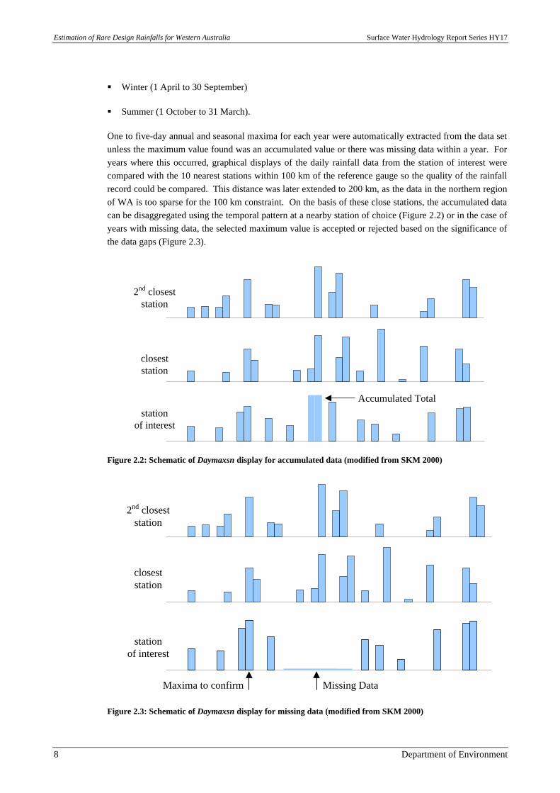
One to five-day annual and seasonal maxima for each year were automatically extracted from the data setunless the maximum value found was an accumulated value or there was missing data within a year. Foryears where this occurred, graphical displays of the daily rainfall data from the station of interest werecompared with the 10 nearest stations within 100 km of the reference gauge so the quality of the rainfallrecord could be compared. This distance was later extended to 200 km, as the data in the northern regionof WA is too sparse for the 100 km constraint. On the basis of these close stations, the accumulated datacan be disaggregated using the temporal pattern at a nearby station of choice (Figure 2.2) or in the case ofyears with missing data, the selected maximum value is accepted or rejected based on the significance ofthe data gaps (Figure 2.3).
stationof interest
closeststation
2nd closeststation
Accumulated Total
Figure 2.2: Schematic of Daymaxsn display for accumulated data (modified from SKM 2000)
stationof interest
closeststation
2nd closeststation
Missing DataMaxima to confirm
Figure 2.3: Schematic of Daymaxsn display for missing data (modified from SKM 2000)
Surface Water Hydrology Report Series HY17 Estimation of Rare Design Rainfalls for Western Australia
Department of Environment 9
This examination of the data highlighted a number of suspicious events in relation to close stations. Ofthese, 141 queries were sent to the Bureau of Meteorology for checking against the original records. Themajority were stations with rainfall depth values significantly higher than those recorded at close stations.95 of the queries checked by the Bureau of Meteorology were found to be incorrect or could not beverified. Typical errors were data incorrectly recorded or processed and accumulated rainfall recordsbeing displayed as one-day rainfall events. These were often stations located along the Rabbit ProofFence line. Isolated thunderstorms or cyclones that were not recorded at close stations typically causedevents that were verified as correct. Isolated rainfalls were difficult to confirm using the program as theclosest stations in the north of WA could typically be up to 200 km away from the gauge of interest dueto the sparse distribution of stations in that region.
As the CRC-FORGE analysis focuses on extremes, the data preparation stage was highly demanding withthe additional extraction of seasonal data. As the highest ranking events can often be less reliable, long,complete and accurate rainfall records were crucial to allow seasonal extraction and to produce a reliablefrequency analysis at each site. Although the program extracted the maximum data automatically, inexcess of 40,000 user judgements were made in relation to accumulated and missing data. As a result,this module of the project was particularly repetitious, labour intensive and time consuming.
2.4 Checking of maxima
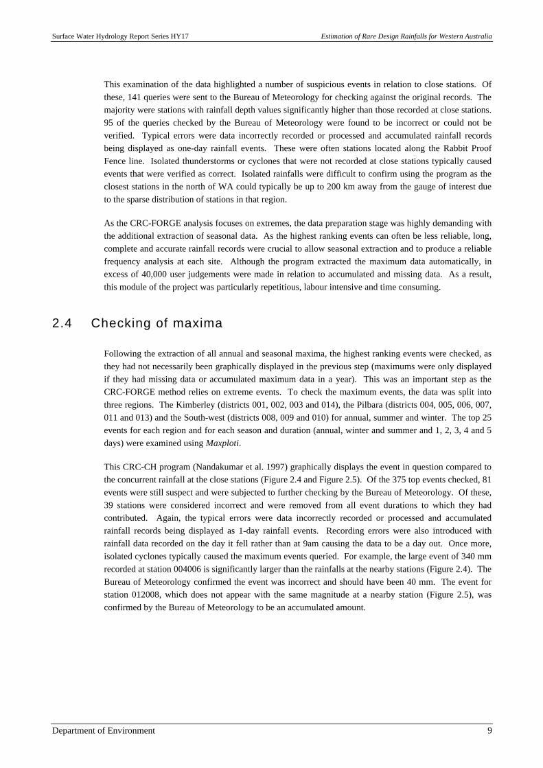
Following the extraction of all annual and seasonal maxima, the highest ranking events were checked, asthey had not necessarily been graphically displayed in the previous step (maximums were only displayedif they had missing data or accumulated maximum data in a year). This was an important step as theCRC-FORGE method relies on extreme events. To check the maximum events, the data was split intothree regions. The Kimberley (districts 001, 002, 003 and 014), the Pilbara (districts 004, 005, 006, 007,011 and 013) and the South-west (districts 008, 009 and 010) for annual, summer and winter. The top 25events for each region and for each season and duration (annual, winter and summer and 1, 2, 3, 4 and 5days) were examined using Maxploti.
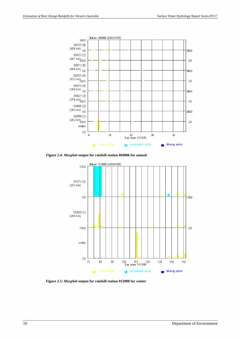
This CRC-CH program (Nandakumar et al. 1997) graphically displays the event in question compared tothe concurrent rainfall at the close stations (Figure 2.4 and Figure 2.5). Of the 375 top events checked, 81events were still suspect and were subjected to further checking by the Bureau of Meteorology. Of these,39 stations were considered incorrect and were removed from all event durations to which they hadcontributed. Again, the typical errors were data incorrectly recorded or processed and accumulatedrainfall records being displayed as 1-day rainfall events. Recording errors were also introduced withrainfall data recorded on the day it fell rather than at 9am causing the data to be a day out. Once more,isolated cyclones typically caused the maximum events queried. For example, the large event of 340 mmrecorded at station 004006 is significantly larger than the rainfalls at the nearby stations (Figure 2.4). TheBureau of Meteorology confirmed the event was incorrect and should have been 40 mm. The event forstation 012008, which does not appear with the same magnitude at a nearby station (Figure 2.5), wasconfirmed by the Bureau of Meteorology to be an accumulated amount.
Estimation of Rare Design Rainfalls for Western Australia Surface Water Hydrology Report Series HY17
10 Department of Environment
Figure 2.4: Maxploti output for rainfall station 004006 for annual
Figure 2.5: Maxploti output for rainfall station 012008 for winter
Surface Water Hydrology Report Series HY17 Estimation of Rare Design Rainfalls for Western Australia
Department of Environment 11
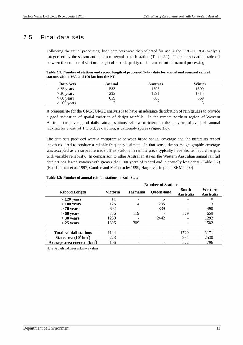
2.5 Final data sets
Following the initial processing, base data sets were then selected for use in the CRC-FORGE analysiscategorised by the season and length of record at each station (Table 2.1). The data sets are a trade offbetween the number of stations, length of record, quality of data and effort of manual processing!
Table 2.1: Number of stations and record length of processed 1-day data for annual and seasonal rainfallstations within WA and 100 km into the NT
Data Sets Annual Summer Winter> 25 years 1583 1593 1600> 30 years 1292 1291 1315> 60 years 659 663 669> 100 years 3 3 3
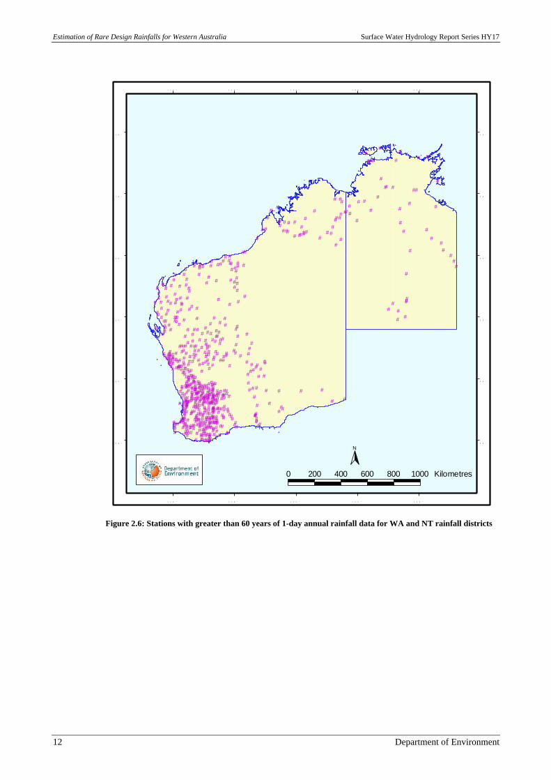
A prerequisite for the CRC-FORGE analysis is to have an adequate distribution of rain gauges to providea good indication of spatial variation of design rainfalls. In the remote northern region of WesternAustralia the coverage of daily rainfall stations, with a sufficient number of years of available annualmaxima for events of 1 to 5 days duration, is extremely sparse (Figure 2.6).
The data sets produced were a compromise between broad spatial coverage and the minimum recordlength required to produce a reliable frequency estimate. In that sense, the sparse geographic coveragewas accepted as a reasonable trade off as stations in remote areas typically have shorter record lengthswith variable reliability. In comparison to other Australian states, the Western Australian annual rainfalldata set has fewer stations with greater than 100 years of record and is spatially less dense (Table 2.2)(Nandakumar et al. 1997, Gamble and McConachy 1999, Hargraves in prep., SKM 2000).
Table 2.2: Number of annual rainfall stations in each State
Number of Stations
Record Length Victoria Tasmania Queensland SouthAustralia
WesternAustralia
> 120 years 11 - 5 - 0> 100 years 176 4 235 - 3> 70 years 602 - 839 - 490> 60 years 756 119 - 529 659> 30 years 1260 - 2442 - 1292> 25 years 1396 309 - 1582
Total rainfall stations 2144 - - 1720 3171State area (103 km2) 228 - - 984 2530
Average area covered (km2) 106 - - 572 796Note: A dash indicates unknown values
Estimation of Rare Design Rainfalls for Western Australia Surface Water Hydrology Report Series HY17
12 Department of Environment
#
#
#
#
#
##
#
##
##
#
###
#
#
#
#
#
##
##
#
#
#
#
#
###
##
#
# #
##
##
#
#
#
##
##
##
#
##
###
# ###
#
## #
#
##
# ##
#
#
#
###
#
## #
#
#
#
##
#
#
#
#
##
##
#
#
#
#
#
#
#
##
#
##
## #
#
#
#
#
#
#
# #
#
#
#
#
#
##
#
##
#
##
#
#
#
#
# #
#
###
#
##
#
#
#
#
#
#
#
#
#
## #
#
#
#
#
#
#
##
#
#
#
#
#
##
#
##
#
#
#
#
##
# #
#
##
#
## #
#
#
#
#
#
#
#
###
#
#
##
#
#
###
#
#
# #
##
#
#
#
#
#
##
#
# #
##
#
#
#
#
##
#
#
#
#
##
#
#
#
#
##
###
#####
##
#
#
## ##
##
#
#
#
##
#
#
#
##
#
#
##
##
##
#
#
#
###
#
#
#
#####
#
##
##
#
#
#
#
#
#
###
##
###
#
##
##
####
#
#
##
##
##
#
#
###
#
#
##
# #
# ####
#
##
#
#
# ## #
## ## ##
#
#
#
#
##
#
#
###
#
##
#
##
#
#
#
#
#
#
#
##
##
#
#
##
#
####
##
## #
###
##
# ##
#
#
##
#
###
#
#
##
####
# ##
#
#
##
##
#
##
##
## ####
## ###
##
#
###
#
##
##
###
## #
#
###
##
#
#
#
#
##
#
#
##
#
##
#
##
#
#
## #
##
#
#
##
#
#### #
##
#
## #
##
#
#
#
##
# #
#
#
##
#
##
#
## ###
##
###
#
# #
#
# ###
#
##
##
#
#
#
#
#
#
# ##
#
#
#
##
#
#
#
##
##
#
#
#
##
#
# #
#
#
#
#
#
#
#
#
##
#
#
#
#
#
# ##
#
#
#
#
#
#
#
#
#
# #
#
##
#
##
###
##
#
#
#
#
##
#
#
#
#
#
##
#
# #
##
##
#
#
#
##
#
#
#
#
##
#
##
#### #
## #
#
#
#
#
##
#
#
##
#
#
#
# #
#
#
#
##
#
#
###
#
#
#
#
#
# #
##
#
##
0 200 400 600 800 1000 Kilometres
N3 5 ° 3 5 °
3 0 ° 3 0 °
2 5 ° 2 5 °
2 0 ° 2 0 °
1 5 ° 1 5 °
1 0 ° 1 0 °
1 1 5 °
1 1 5 °
1 2 0 °
1 2 0 °
1 2 5 °
1 2 5 °
1 3 0 °
1 3 0 °
1 3 5 °
1 3 5 °
Figure 2.6: Stations with greater than 60 years of 1-day annual rainfall data for WA and NT rainfall districts
Surface Water Hydrology Report Series HY17 Estimation of Rare Design Rainfalls for Western Australia
Department of Environment 13
3 Identification of distributions andhomogeneous regions
A key assumption of regional methods is that the data in a region is homogeneous with respect to time(stationarity) and space (regional homogeneity) (Hosking and Wallis 1991).
3.1 Stationarity
Two stationarity tests supplied by the CRC-CH were applied to the 1-day duration annual and seasonalmaxima series at sites with greater than 25 years of data. The Mann-Kendall rank correlation test(Srikanthan and Stewart 1991) and the distribution-free CUSUM test (McGilchrist and Woodeyer 1975)were used. The tests were undertaken at the 5% significance level (Table 3.1).
Table 3.1: Number and percentage of stations that failed the Mann-Kendall and CUSUM tests
No. ofStations
FailedMann-Kendall
Failed(%)
FailedCUSUM
Failed(%)
Failed bothtests
Failed(%)
Annual 1583 92 6% 137 9% 29 2%Summer 1593 83 5% 71 4% 20 1%Winter 1600 127 8% 160 10% 49 3%
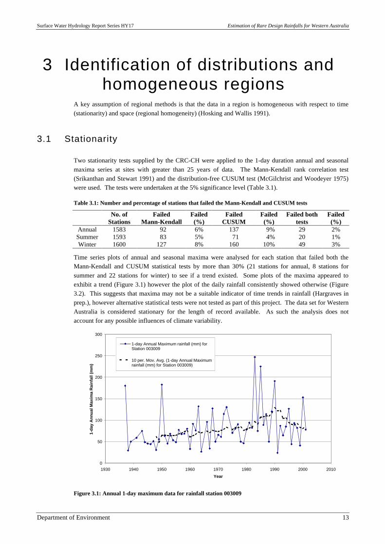
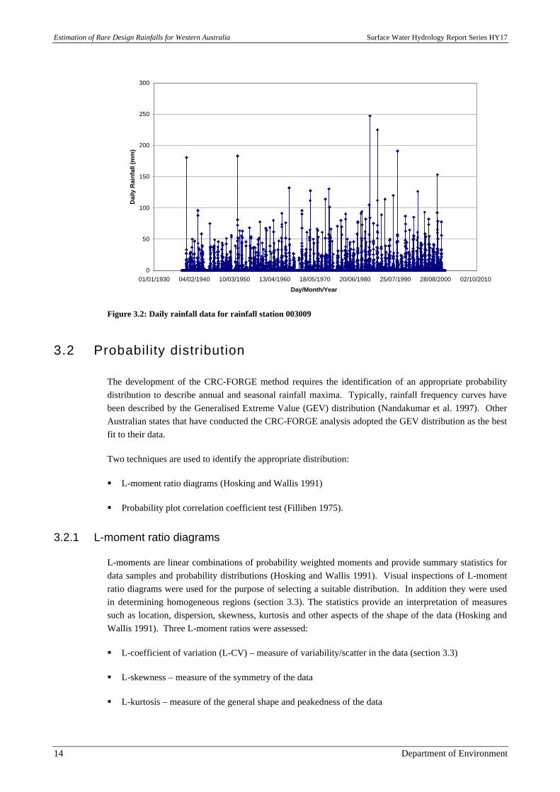
Time series plots of annual and seasonal maxima were analysed for each station that failed both theMann-Kendall and CUSUM statistical tests by more than 30% (21 stations for annual, 8 stations forsummer and 22 stations for winter) to see if a trend existed. Some plots of the maxima appeared toexhibit a trend (Figure 3.1) however the plot of the daily rainfall consistently showed otherwise (Figure3.2). This suggests that maxima may not be a suitable indicator of time trends in rainfall (Hargraves inprep.), however alternative statistical tests were not tested as part of this project. The data set for WesternAustralia is considered stationary for the length of record available. As such the analysis does notaccount for any possible influences of climate variability.
0
50
100
150
200
250
300
1930 1940 1950 1960 1970 1980 1990 2000 2010
Year
1-d
ay A
nn
ual
Max
ima
Rai
nfa
ll (m
m)
1-day Annual Maximum rainfall (mm) forStation 003009
10 per. Mov. Avg. (1-day Annual Maximumrainfall (mm) for Station 003009)
Figure 3.1: Annual 1-day maximum data for rainfall station 003009
Estimation of Rare Design Rainfalls for Western Australia Surface Water Hydrology Report Series HY17
14 Department of Environment
0
50
100
150
200
250
300
01/01/1930 04/02/1940 10/03/1950 13/04/1960 18/05/1970 20/06/1980 25/07/1990 28/08/2000 02/10/2010
Day/Month/Year
Dai
ly R
ain
fall
(mm
)
Figure 3.2: Daily rainfall data for rainfall station 003009
3.2 Probability distribution
The development of the CRC-FORGE method requires the identification of an appropriate probabilitydistribution to describe annual and seasonal rainfall maxima. Typically, rainfall frequency curves havebeen described by the Generalised Extreme Value (GEV) distribution (Nandakumar et al. 1997). OtherAustralian states that have conducted the CRC-FORGE analysis adopted the GEV distribution as the bestfit to their data.
Two techniques are used to identify the appropriate distribution:
§ L-moment ratio diagrams (Hosking and Wallis 1991)
§ Probability plot correlation coefficient test (Filliben 1975).
3.2.1 L-moment ratio diagrams
L-moments are linear combinations of probability weighted moments and provide summary statistics fordata samples and probability distributions (Hosking and Wallis 1991). Visual inspections of L-momentratio diagrams were used for the purpose of selecting a suitable distribution. In addition they were usedin determining homogeneous regions (section 3.3). The statistics provide an interpretation of measuressuch as location, dispersion, skewness, kurtosis and other aspects of the shape of the data (Hosking andWallis 1991). Three L-moment ratios were assessed:
§ L-coefficient of variation (L-CV) – measure of variability/scatter in the data (section 3.3)
§ L-skewness – measure of the symmetry of the data
§ L-kurtosis – measure of the general shape and peakedness of the data
Surface Water Hydrology Report Series HY17 Estimation of Rare Design Rainfalls for Western Australia
Department of Environment 15
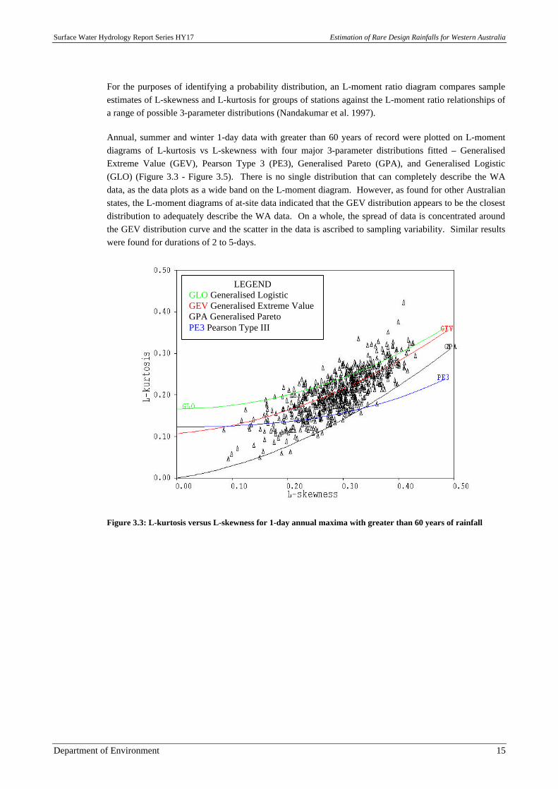
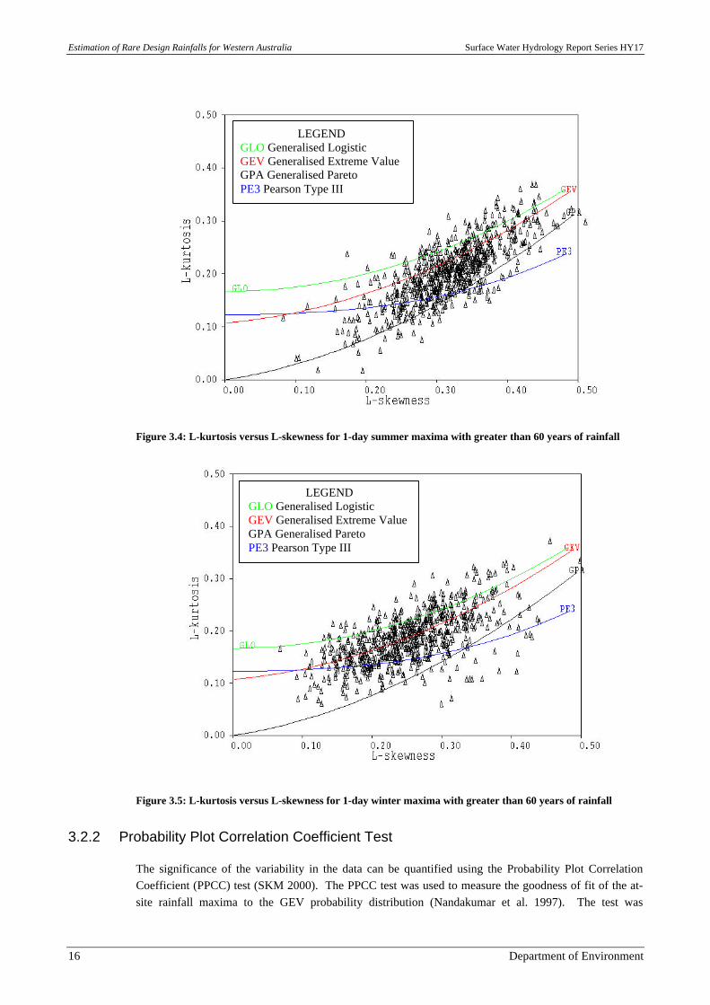
For the purposes of identifying a probability distribution, an L-moment ratio diagram compares sampleestimates of L-skewness and L-kurtosis for groups of stations against the L-moment ratio relationships ofa range of possible 3-parameter distributions (Nandakumar et al. 1997).
Annual, summer and winter 1-day data with greater than 60 years of record were plotted on L-momentdiagrams of L-kurtosis vs L-skewness with four major 3-parameter distributions fitted – GeneralisedExtreme Value (GEV), Pearson Type 3 (PE3), Generalised Pareto (GPA), and Generalised Logistic(GLO) (Figure 3.3 - Figure 3.5). There is no single distribution that can completely describe the WAdata, as the data plots as a wide band on the L-moment diagram. However, as found for other Australianstates, the L-moment diagrams of at-site data indicated that the GEV distribution appears to be the closestdistribution to adequately describe the WA data. On a whole, the spread of data is concentrated aroundthe GEV distribution curve and the scatter in the data is ascribed to sampling variability. Similar resultswere found for durations of 2 to 5-days.
LEGENDGLO Generalised LogisticGEV Generalised Extreme ValueGPA Generalised ParetoPE3 Pearson Type III
Figure 3.3: L-kurtosis versus L-skewness for 1-day annual maxima with greater than 60 years of rainfall
Estimation of Rare Design Rainfalls for Western Australia Surface Water Hydrology Report Series HY17
16 Department of Environment
LEGENDGLO Generalised LogisticGEV Generalised Extreme ValueGPA Generalised ParetoPE3 Pearson Type III
Figure 3.4: L-kurtosis versus L-skewness for 1-day summer maxima with greater than 60 years of rainfall
LEGENDGLO Generalised LogisticGEV Generalised Extreme ValueGPA Generalised ParetoPE3 Pearson Type III
Figure 3.5: L-kurtosis versus L-skewness for 1-day winter maxima with greater than 60 years of rainfall
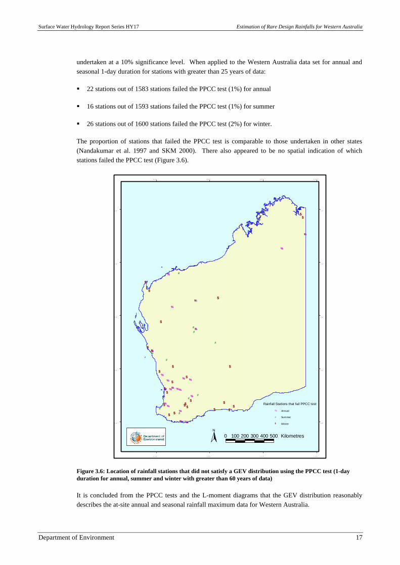
3.2.2 Probability Plot Correlation Coefficient Test
The significance of the variability in the data can be quantified using the Probability Plot CorrelationCoefficient (PPCC) test (SKM 2000). The PPCC test was used to measure the goodness of fit of the at-site rainfall maxima to the GEV probability distribution (Nandakumar et al. 1997). The test was
Surface Water Hydrology Report Series HY17 Estimation of Rare Design Rainfalls for Western Australia
Department of Environment 17
undertaken at a 10% significance level. When applied to the Western Australia data set for annual andseasonal 1-day duration for stations with greater than 25 years of data:
§ 22 stations out of 1583 stations failed the PPCC test (1%) for annual
§ 16 stations out of 1593 stations failed the PPCC test (1%) for summer
§ 26 stations out of 1600 stations failed the PPCC test (2%) for winter.
The proportion of stations that failed the PPCC test is comparable to those undertaken in other states(Nandakumar et al. 1997 and SKM 2000). There also appeared to be no spatial indication of whichstations failed the PPCC test (Figure 3.6).
$$
$
$
$
$
$
$
$$
$
$
$$ $
$
$$
$$$
$
$
$$
$
#
#
#
#
#
#
#
#
# #
#
#
#
##
#
%
%
%
%
%
%
%
%
%
% %
% %
%%
% %
%%
%
%
%
%
%
%
%
%
%
%
%
%
% %
% %
%%
% %
%%
%
%
%
#
#
#
#
#
#
#
#
# #
#
#
#
##
#
$$
$
$
$
$
$
$
$$
$
$
$$ $
$
$
$
$$$
$
$
$$
$
3 5 ° 3 5 °
3 0 ° 3 0 °
2 5 ° 2 5 °
2 0 ° 2 0 °
1 5 ° 1 5 °
1 1 5 °
1 1 5 °
1 2 0 °
1 2 0 °
1 2 5 °
1 2 5 °
1 3 0 °
1 3 0 °
0 100 200 300 400 500 KilometresN
Annual%
Summer#
Winter$
Rainfall Stations that fail PPCC test
Figure 3.6: Location of rainfall stations that did not satisfy a GEV distribution using the PPCC test (1-dayduration for annual, summer and winter with greater than 60 years of data)
It is concluded from the PPCC tests and the L-moment diagrams that the GEV distribution reasonablydescribes the at-site annual and seasonal rainfall maximum data for Western Australia.
Estimation of Rare Design Rainfalls for Western Australia Surface Water Hydrology Report Series HY17
18 Department of Environment
3.3 Homogeneity
A condition for the application of regional frequency analysis methods such as CRC-FORGE is that thedata from different sites within a region show a satisfactory degree of homogeneity. This was tested byproposing preliminary regions and applying statistical homogeneity tests to assess whether the datawithin each of the regions satisfies the homogeneity criteria.
The acceptability of a region’s homogeneity was determined using statistics by Lu and Stedinger (1992)and Hosking and Wallis (1991). Analysis was focused on L-moment ratio statistics and diagrams(section 3.2.1). The Hosking and Wallis (1991) test is based on the comparison between variations insample L-moments of the sites in the region with the variations that would be expected for ahomogeneous region having the same population L-moments. Two criteria were assessed:
§ The standard deviation of L-CV
§ Visual inspection of L-moment ratio diagrams.
The simplest, and most important, measure of variation between sites is H1, which relates to the standarddeviation of L-CV (Hosking and Wallis 1991), as it has the most power in differentiating betweenhomogeneous and heterogeneous regions, with lower values of H1 indicating greater homogeneity.
Visual inspections of L-moment ratio diagrams were used for the purpose of evaluating regions(Nandakumar et al. 1997). The plots of L-moment ratios used were combinations of L-skewness/L-kurtosis and L-CV/L-skewness.
3.3.1 Preliminary regions for Western Australia
Homogeneity testing for Western Australia was conducted on an annual and seasonal basis for data withgreater than 60 years of record and 1-day duration. The first proposed region covered the whole of WA,and it was found that the annual and seasonal maximum data was not statistically one homogeneousregion for any rainfall duration. This was confirmed by the Lu and Stedinger (1992) and Hosking andWallis (1991) tests. As a result it was necessary to identify smaller regions within WA that satisfied thecriterion of homogeneity.
Regions were defined according to the Bureau of Meteorology rainfall districts (Figure 1.1) and initiallyeach district was tested independently for homogeneity. This showed that the individual rainfall districtscould not be considered homogeneous with only 5 districts out of 15 (for annual 1-day data with greaterthan 60 years of record) convincingly passing the criteria for homogeneity based on the standarddeviation of L-CV. Despite a number of the individual WA rainfall districts being heterogeneous, furthergroupings were investigated.
In grouping districts together, statistically homogeneous regions could be generated from the tests byplacing stations from across the State in one region. However, these groupings were meteorologicallyinconsistent, so it was decided to place greater importance on the meteorological homogeneity of the datarather than the statistical homogeneity. This took into account such factors as:
§ Storm types (e.g. frontal rain, rain from decaying storms of tropical origin and local thunderstorms)
§ Seasonal variations in storms
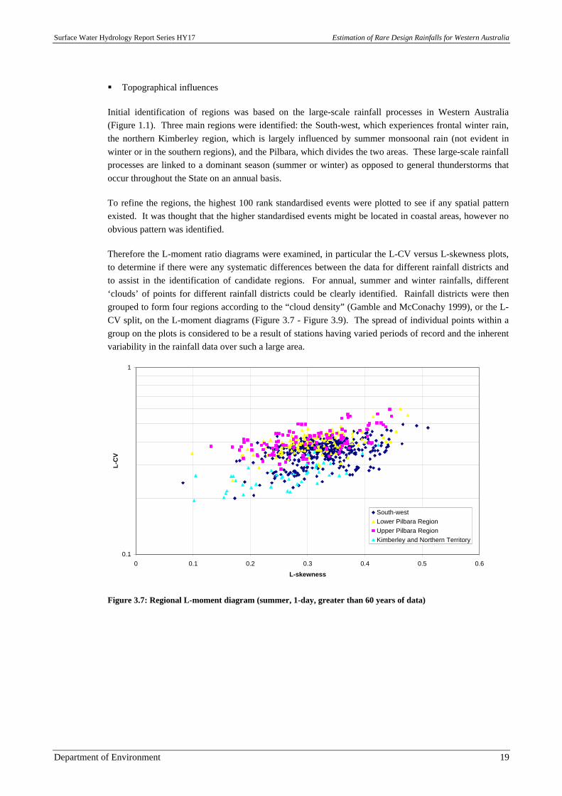
Surface Water Hydrology Report Series HY17 Estimation of Rare Design Rainfalls for Western Australia
Department of Environment 19
§ Topographical influences
Initial identification of regions was based on the large-scale rainfall processes in Western Australia(Figure 1.1). Three main regions were identified: the South-west, which experiences frontal winter rain,the northern Kimberley region, which is largely influenced by summer monsoonal rain (not evident inwinter or in the southern regions), and the Pilbara, which divides the two areas. These large-scale rainfallprocesses are linked to a dominant season (summer or winter) as opposed to general thunderstorms thatoccur throughout the State on an annual basis.
To refine the regions, the highest 100 rank standardised events were plotted to see if any spatial patternexisted. It was thought that the higher standardised events might be located in coastal areas, however noobvious pattern was identified.
Therefore the L-moment ratio diagrams were examined, in particular the L-CV versus L-skewness plots,to determine if there were any systematic differences between the data for different rainfall districts andto assist in the identification of candidate regions. For annual, summer and winter rainfalls, different‘clouds’ of points for different rainfall districts could be clearly identified. Rainfall districts were thengrouped to form four regions according to the “cloud density” (Gamble and McConachy 1999), or the L-CV split, on the L-moment diagrams (Figure 3.7 - Figure 3.9). The spread of individual points within agroup on the plots is considered to be a result of stations having varied periods of record and the inherentvariability in the rainfall data over such a large area.
0.1
1
0 0.1 0.2 0.3 0.4 0.5 0.6
L-skewness
L-C
V
South-westLower Pilbara RegionUpper Pilbara RegionKimberley and Northern Territory
Figure 3.7: Regional L-moment diagram (summer, 1-day, greater than 60 years of data)
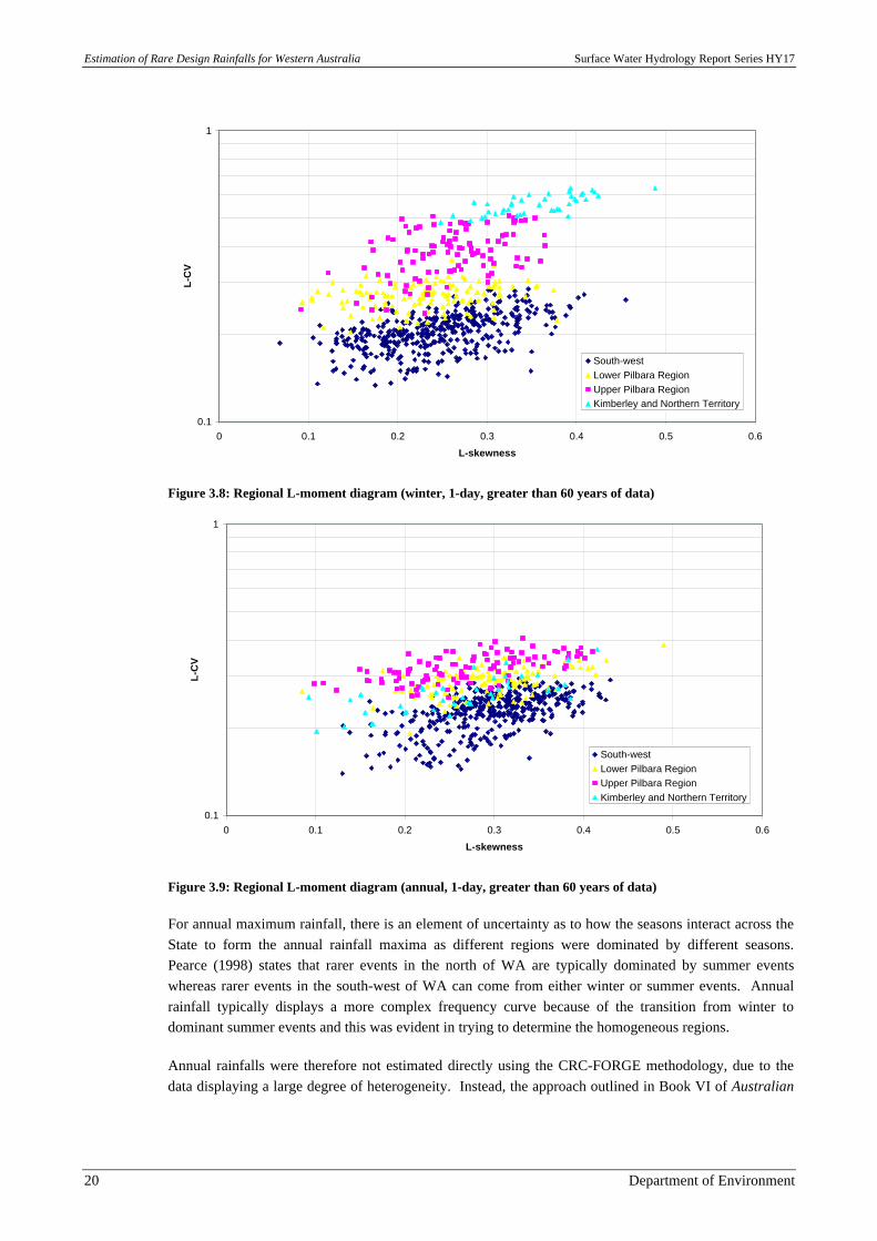
Estimation of Rare Design Rainfalls for Western Australia Surface Water Hydrology Report Series HY17
20 Department of Environment
0.1
1
0 0.1 0.2 0.3 0.4 0.5 0.6
L-skewness
L-C
V
South-westLower Pilbara RegionUpper Pilbara RegionKimberley and Northern Territory
Figure 3.8: Regional L-moment diagram (winter, 1-day, greater than 60 years of data)
0.1
1
0 0.1 0.2 0.3 0.4 0.5 0.6
L-skewness
L-C
V
South-westLower Pilbara RegionUpper Pilbara RegionKimberley and Northern Territory
Figure 3.9: Regional L-moment diagram (annual, 1-day, greater than 60 years of data)
For annual maximum rainfall, there is an element of uncertainty as to how the seasons interact across theState to form the annual rainfall maxima as different regions were dominated by different seasons.Pearce (1998) states that rarer events in the north of WA are typically dominated by summer eventswhereas rarer events in the south-west of WA can come from either winter or summer events. Annualrainfall typically displays a more complex frequency curve because of the transition from winter todominant summer events and this was evident in trying to determine the homogeneous regions.
Annual rainfalls were therefore not estimated directly using the CRC-FORGE methodology, due to thedata displaying a large degree of heterogeneity. Instead, the approach outlined in Book VI of Australian
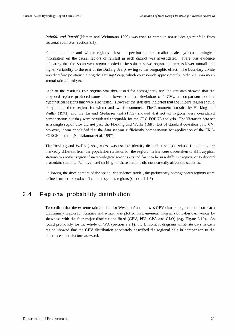
Surface Water Hydrology Report Series HY17 Estimation of Rare Design Rainfalls for Western Australia
Department of Environment 21
Rainfall and Runoff (Nathan and Weinmann 1999) was used to compute annual design rainfalls fromseasonal estimates (section 5.3).
For the summer and winter regions, closer inspection of the smaller scale hydrometeorologicalinformation on the causal factors of rainfall in each district was investigated. There was evidenceindicating that the South-west region needed to be split into two regions as there is lower rainfall andhigher variability to the east of the Darling Scarp, owing to the orographic effect. The boundary dividewas therefore positioned along the Darling Scarp, which corresponds approximately to the 700 mm meanannual rainfall isohyet.
Each of the resulting five regions was then tested for homogeneity and the statistics showed that theproposed regions produced some of the lowest standard deviations of L-CVs, in comparison to otherhypothetical regions that were also tested. However the statistics indicated that the Pilbara region shouldbe split into three regions for winter and two for summer. The L-moment statistics by Hosking andWallis (1991) and the Lu and Stedinger test (1992) showed that not all regions were consideredhomogeneous but they were considered acceptable for the CRC-FORGE analysis. The Victorian data setas a single region also did not pass the Hosking and Wallis (1991) test of standard deviation of L-CV,however, it was concluded that the data set was sufficiently homogeneous for application of the CRC-FORGE method (Nandakumar et al. 1997).
The Hosking and Wallis (1991) x-test was used to identify discordant stations whose L-moments aremarkedly different from the population statistics for the region. Trials were undertaken to shift atypicalstations to another region if meteorological reasons existed for it to be in a different region, or to discarddiscordant stations. Removal, and shifting, of these stations did not markedly affect the statistics.
Following the development of the spatial dependence model, the preliminary homogeneous regions wererefined further to produce final homogenous regions (section 4.1.3).
3.4 Regional probability distribution
To confirm that the extreme rainfall data for Western Australia was GEV distributed, the data from eachpreliminary region for summer and winter was plotted on L-moment diagrams of L-kurtosis versus L-skewness with the four major distributions fitted (GEV, PE3, GPA and GLO) (e.g. Figure 3.10). Asfound previously for the whole of WA (section 3.2.1), the L-moment diagrams of at-site data in eachregion showed that the GEV distribution adequately described the regional data in comparison to theother three distributions assessed.
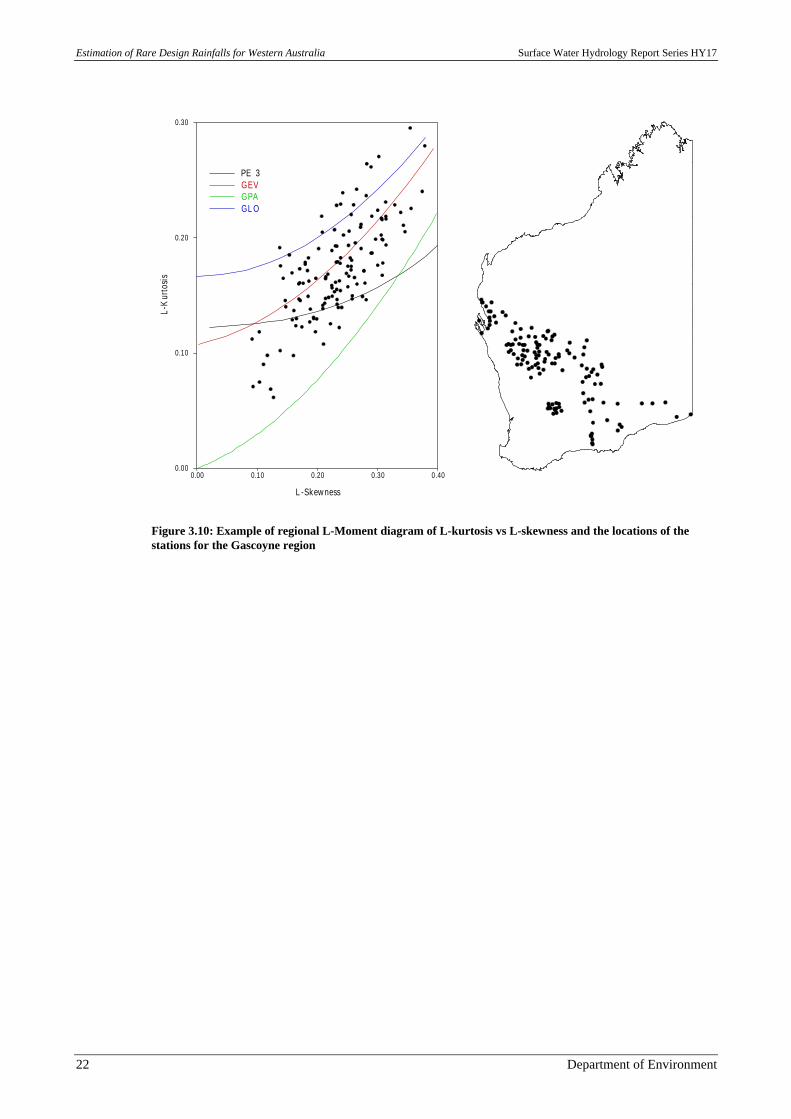
Estimation of Rare Design Rainfalls for Western Australia Surface Water Hydrology Report Series HY17
22 Department of Environment
0.00
0.10
0.20
0.30
L-K
urto
sis
0.00 0.10 0.20 0.30 0.40
L -Skew ness
PE 3GEVGPAGL O
Figure 3.10: Example of regional L-Moment diagram of L-kurtosis vs L-skewness and the locations of thestations for the Gascoyne region
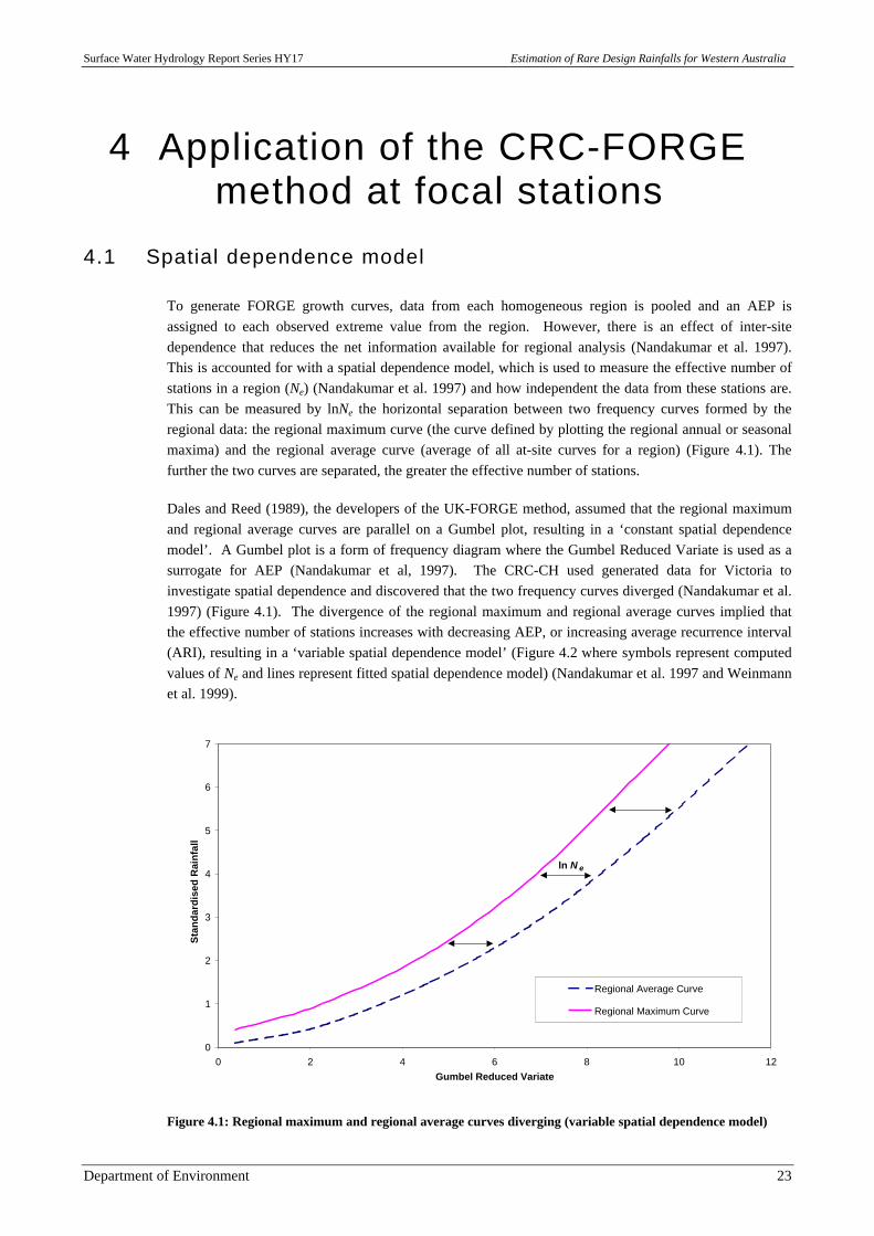
Surface Water Hydrology Report Series HY17 Estimation of Rare Design Rainfalls for Western Australia
Department of Environment 23
4 Application of the CRC-FORGEmethod at focal stations
4.1 Spatial dependence model
To generate FORGE growth curves, data from each homogeneous region is pooled and an AEP isassigned to each observed extreme value from the region. However, there is an effect of inter-sitedependence that reduces the net information available for regional analysis (Nandakumar et al. 1997).This is accounted for with a spatial dependence model, which is used to measure the effective number ofstations in a region (Ne) (Nandakumar et al. 1997) and how independent the data from these stations are.This can be measured by lnNe the horizontal separation between two frequency curves formed by theregional data: the regional maximum curve (the curve defined by plotting the regional annual or seasonalmaxima) and the regional average curve (average of all at-site curves for a region) (Figure 4.1). Thefurther the two curves are separated, the greater the effective number of stations.
Dales and Reed (1989), the developers of the UK-FORGE method, assumed that the regional maximumand regional average curves are parallel on a Gumbel plot, resulting in a ‘constant spatial dependencemodel’. A Gumbel plot is a form of frequency diagram where the Gumbel Reduced Variate is used as asurrogate for AEP (Nandakumar et al, 1997). The CRC-CH used generated data for Victoria toinvestigate spatial dependence and discovered that the two frequency curves diverged (Nandakumar et al.1997) (Figure 4.1). The divergence of the regional maximum and regional average curves implied thatthe effective number of stations increases with decreasing AEP, or increasing average recurrence interval(ARI), resulting in a ‘variable spatial dependence model’ (Figure 4.2 where symbols represent computedvalues of Ne and lines represent fitted spatial dependence model) (Nandakumar et al. 1997 and Weinmannet al. 1999).
0
1
2
3
4
5
6
7
0 2 4 6 8 10 12Gumbel Reduced Variate
Sta
nd
ard
ised
Rai
nfa
ll
Regional Average Curve
Regional Maximum Curve
ln N e
Figure 4.1: Regional maximum and regional average curves diverging (variable spatial dependence model)
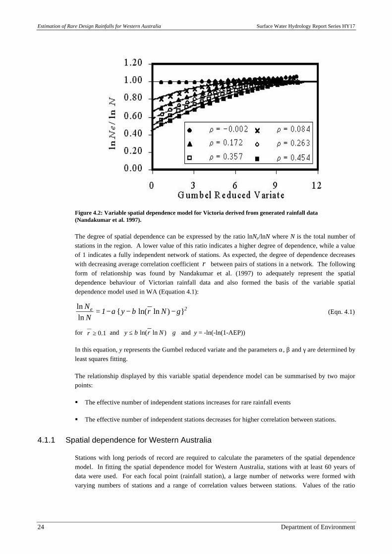
Estimation of Rare Design Rainfalls for Western Australia Surface Water Hydrology Report Series HY17
24 Department of Environment
Figure 4.2: Variable spatial dependence model for Victoria derived from generated rainfall data(Nandakumar et al. 1997).
The degree of spatial dependence can be expressed by the ratio lnNe/lnN where N is the total number ofstations in the region. A lower value of this ratio indicates a higher degree of dependence, while a valueof 1 indicates a fully independent network of stations. As expected, the degree of dependence decreaseswith decreasing average correlation coefficient ρ between pairs of stations in a network. The followingform of relationship was found by Nandakumar et al. (1997) to adequately represent the spatialdependence behaviour of Victorian rainfall data and also formed the basis of the variable spatialdependence model used in WA (Equation 4.1):
2e Ny1NN
})lnln({lnln
γρβα −−−= (Eqn. 4.1)
for 1.0≥ρ and γρβ +≤ )lnln( Ny and y = -ln(-ln(1-AEP))
In this equation, y represents the Gumbel reduced variate and the parameters α, β and γ are determined byleast squares fitting.
The relationship displayed by this variable spatial dependence model can be summarised by two majorpoints:
§ The effective number of independent stations increases for rare rainfall events
§ The effective number of independent stations decreases for higher correlation between stations.
4.1.1 Spatial dependence for Western Australia
Stations with long periods of record are required to calculate the parameters of the spatial dependencemodel. In fitting the spatial dependence model for Western Australia, stations with at least 60 years ofdata were used. For each focal point (rainfall station), a large number of networks were formed withvarying numbers of stations and a range of correlation values between stations. Values of the ratio
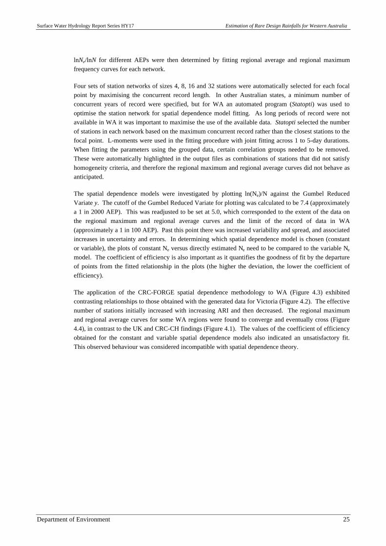
Surface Water Hydrology Report Series HY17 Estimation of Rare Design Rainfalls for Western Australia
Department of Environment 25
lnNe/lnN for different AEPs were then determined by fitting regional average and regional maximumfrequency curves for each network.
Four sets of station networks of sizes 4, 8, 16 and 32 stations were automatically selected for each focalpoint by maximising the concurrent record length. In other Australian states, a minimum number ofconcurrent years of record were specified, but for WA an automated program (Statopti) was used tooptimise the station network for spatial dependence model fitting. As long periods of record were notavailable in WA it was important to maximise the use of the available data. Statopti selected the numberof stations in each network based on the maximum concurrent record rather than the closest stations to thefocal point. L-moments were used in the fitting procedure with joint fitting across 1 to 5-day durations.When fitting the parameters using the grouped data, certain correlation groups needed to be removed.These were automatically highlighted in the output files as combinations of stations that did not satisfyhomogeneity criteria, and therefore the regional maximum and regional average curves did not behave asanticipated.
The spatial dependence models were investigated by plotting ln(Ne)/N against the Gumbel ReducedVariate y. The cutoff of the Gumbel Reduced Variate for plotting was calculated to be 7.4 (approximatelya 1 in 2000 AEP). This was readjusted to be set at 5.0, which corresponded to the extent of the data onthe regional maximum and regional average curves and the limit of the record of data in WA(approximately a 1 in 100 AEP). Past this point there was increased variability and spread, and associatedincreases in uncertainty and errors. In determining which spatial dependence model is chosen (constantor variable), the plots of constant Ne versus directly estimated Ne need to be compared to the variable Ne
model. The coefficient of efficiency is also important as it quantifies the goodness of fit by the departureof points from the fitted relationship in the plots (the higher the deviation, the lower the coefficient ofefficiency).
The application of the CRC-FORGE spatial dependence methodology to WA (Figure 4.3) exhibitedcontrasting relationships to those obtained with the generated data for Victoria (Figure 4.2). The effectivenumber of stations initially increased with increasing ARI and then decreased. The regional maximumand regional average curves for some WA regions were found to converge and eventually cross (Figure4.4), in contrast to the UK and CRC-CH findings (Figure 4.1). The values of the coefficient of efficiencyobtained for the constant and variable spatial dependence models also indicated an unsatisfactory fit.This observed behaviour was considered incompatible with spatial dependence theory.
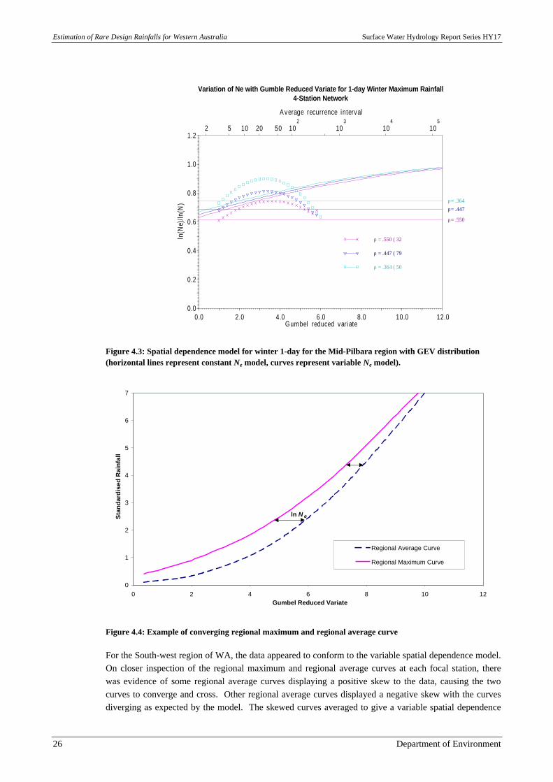
Estimation of Rare Design Rainfalls for Western Australia Surface Water Hydrology Report Series HY17
26 Department of Environment
0.0 2.0 4.0 6.0 8.0 10.0 12.0Gumbel reduced variate
2 5 10 20 50 102
103
104
105
A verage recurrence interval
0.0
0.2
0.4
0.6
0.8
1.0
1.2
ln(N
e)/ln
(N)
Variation of Ne with Gumble Reduced Variate for 1-day Winter Maximum Rainfall4-Station Network
ρ = .550 ( 32)
ρ= .550
ρ = .447 ( 79)
ρ= .447
ρ = .364 ( 50)
ρ= .364
Figure 4.3: Spatial dependence model for winter 1-day for the Mid-Pilbara region with GEV distribution(horizontal lines represent constant Ne model, curves represent variable Ne model).
0
1
2
3
4
5
6
7
0 2 4 6 8 10 12Gumbel Reduced Variate
Sta
nd
ard
ised
Rai
nfa
ll
Regional Average Curve
Regional Maximum Curve
ln N e
Figure 4.4: Example of converging regional maximum and regional average curve
For the South-west region of WA, the data appeared to conform to the variable spatial dependence model.On closer inspection of the regional maximum and regional average curves at each focal station, therewas evidence of some regional average curves displaying a positive skew to the data, causing the twocurves to converge and cross. Other regional average curves displayed a negative skew with the curvesdiverging as expected by the model. The skewed curves averaged to give a variable spatial dependence
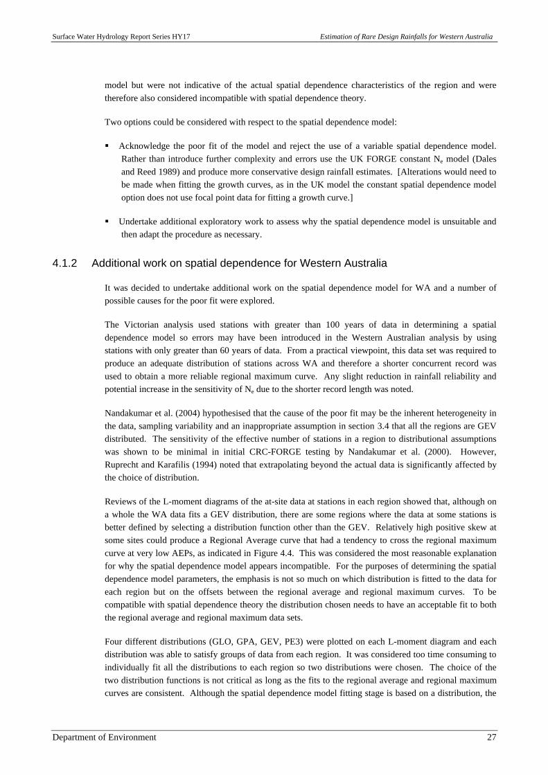
Surface Water Hydrology Report Series HY17 Estimation of Rare Design Rainfalls for Western Australia
Department of Environment 27
model but were not indicative of the actual spatial dependence characteristics of the region and weretherefore also considered incompatible with spatial dependence theory.
Two options could be considered with respect to the spatial dependence model:
§ Acknowledge the poor fit of the model and reject the use of a variable spatial dependence model.Rather than introduce further complexity and errors use the UK FORGE constant Ne model (Dalesand Reed 1989) and produce more conservative design rainfall estimates. [Alterations would need tobe made when fitting the growth curves, as in the UK model the constant spatial dependence modeloption does not use focal point data for fitting a growth curve.]
§ Undertake additional exploratory work to assess why the spatial dependence model is unsuitable andthen adapt the procedure as necessary.
4.1.2 Additional work on spatial dependence for Western Australia
It was decided to undertake additional work on the spatial dependence model for WA and a number ofpossible causes for the poor fit were explored.
The Victorian analysis used stations with greater than 100 years of data in determining a spatialdependence model so errors may have been introduced in the Western Australian analysis by usingstations with only greater than 60 years of data. From a practical viewpoint, this data set was required toproduce an adequate distribution of stations across WA and therefore a shorter concurrent record wasused to obtain a more reliable regional maximum curve. Any slight reduction in rainfall reliability andpotential increase in the sensitivity of Ne due to the shorter record length was noted.
Nandakumar et al. (2004) hypothesised that the cause of the poor fit may be the inherent heterogeneity inthe data, sampling variability and an inappropriate assumption in section 3.4 that all the regions are GEVdistributed. The sensitivity of the effective number of stations in a region to distributional assumptionswas shown to be minimal in initial CRC-FORGE testing by Nandakumar et al. (2000). However,Ruprecht and Karafilis (1994) noted that extrapolating beyond the actual data is significantly affected bythe choice of distribution.
Reviews of the L-moment diagrams of the at-site data at stations in each region showed that, although ona whole the WA data fits a GEV distribution, there are some regions where the data at some stations isbetter defined by selecting a distribution function other than the GEV. Relatively high positive skew atsome sites could produce a Regional Average curve that had a tendency to cross the regional maximumcurve at very low AEPs, as indicated in Figure 4.4. This was considered the most reasonable explanationfor why the spatial dependence model appears incompatible. For the purposes of determining the spatialdependence model parameters, the emphasis is not so much on which distribution is fitted to the data foreach region but on the offsets between the regional average and regional maximum curves. To becompatible with spatial dependence theory the distribution chosen needs to have an acceptable fit to boththe regional average and regional maximum data sets.
Four different distributions (GLO, GPA, GEV, PE3) were plotted on each L-moment diagram and eachdistribution was able to satisfy groups of data from each region. It was considered too time consuming toindividually fit all the distributions to each region so two distributions were chosen. The choice of thetwo distribution functions is not critical as long as the fits to the regional average and regional maximumcurves are consistent. Although the spatial dependence model fitting stage is based on a distribution, the
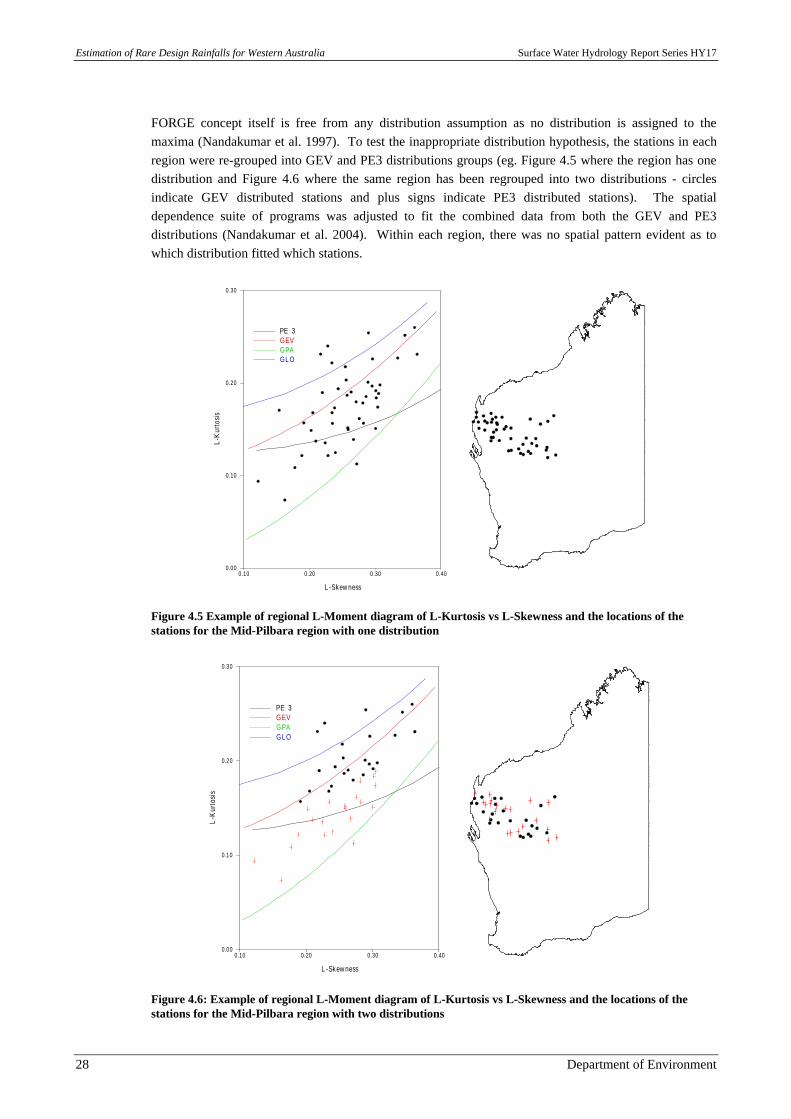
Estimation of Rare Design Rainfalls for Western Australia Surface Water Hydrology Report Series HY17
28 Department of Environment
FORGE concept itself is free from any distribution assumption as no distribution is assigned to themaxima (Nandakumar et al. 1997). To test the inappropriate distribution hypothesis, the stations in eachregion were re-grouped into GEV and PE3 distributions groups (eg. Figure 4.5 where the region has onedistribution and Figure 4.6 where the same region has been regrouped into two distributions - circlesindicate GEV distributed stations and plus signs indicate PE3 distributed stations). The spatialdependence suite of programs was adjusted to fit the combined data from both the GEV and PE3distributions (Nandakumar et al. 2004). Within each region, there was no spatial pattern evident as towhich distribution fitted which stations.
0.00
0.10
0.20
0.30
L-K
urto
sis
0.10 0.20 0.30 0.40
L -Skew ness
PE 3GEVGPAGL O
Figure 4.5 Example of regional L-Moment diagram of L-Kurtosis vs L-Skewness and the locations of thestations for the Mid-Pilbara region with one distribution
0.00
0.10
0.20
0.30
L-K
urto
sis
0.10 0.20 0.30 0.40
L -Skew ness
PE 3GEVGPAGL O
Figure 4.6: Example of regional L-Moment diagram of L-Kurtosis vs L-Skewness and the locations of thestations for the Mid-Pilbara region with two distributions
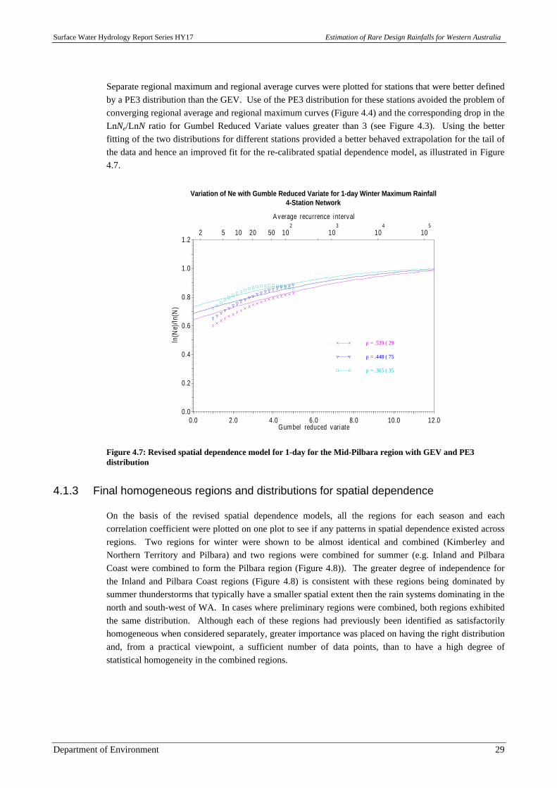
Surface Water Hydrology Report Series HY17 Estimation of Rare Design Rainfalls for Western Australia
Department of Environment 29
Separate regional maximum and regional average curves were plotted for stations that were better definedby a PE3 distribution than the GEV. Use of the PE3 distribution for these stations avoided the problem ofconverging regional average and regional maximum curves (Figure 4.4) and the corresponding drop in theLnNe/LnN ratio for Gumbel Reduced Variate values greater than 3 (see Figure 4.3). Using the betterfitting of the two distributions for different stations provided a better behaved extrapolation for the tail ofthe data and hence an improved fit for the re-calibrated spatial dependence model, as illustrated in Figure4.7.
0.0 2.0 4.0 6.0 8.0 10.0 12.0Gumbel reduced variate
2 5 10 20 50 102
103
104
105
A verage recurrence interval
0.0
0.2
0.4
0.6
0.8
1.0
1.2
ln(N
e)/ln
(N)
Variation of Ne with Gumble Reduced Variate for 1-day Winter Maximum Rainfall4-Station Network
ρ = .539 ( 29)
ρ = .448 ( 75)
ρ = .365 ( 35)
Figure 4.7: Revised spatial dependence model for 1-day for the Mid-Pilbara region with GEV and PE3distribution
4.1.3 Final homogeneous regions and distributions for spatial dependence
On the basis of the revised spatial dependence models, all the regions for each season and eachcorrelation coefficient were plotted on one plot to see if any patterns in spatial dependence existed acrossregions. Two regions for winter were shown to be almost identical and combined (Kimberley andNorthern Territory and Pilbara) and two regions were combined for summer (e.g. Inland and PilbaraCoast were combined to form the Pilbara region (Figure 4.8)). The greater degree of independence forthe Inland and Pilbara Coast regions (Figure 4.8) is consistent with these regions being dominated bysummer thunderstorms that typically have a smaller spatial extent then the rain systems dominating in thenorth and south-west of WA. In cases where preliminary regions were combined, both regions exhibitedthe same distribution. Although each of these regions had previously been identified as satisfactorilyhomogeneous when considered separately, greater importance was placed on having the right distributionand, from a practical viewpoint, a sufficient number of data points, than to have a high degree ofstatistical homogeneity in the combined regions.
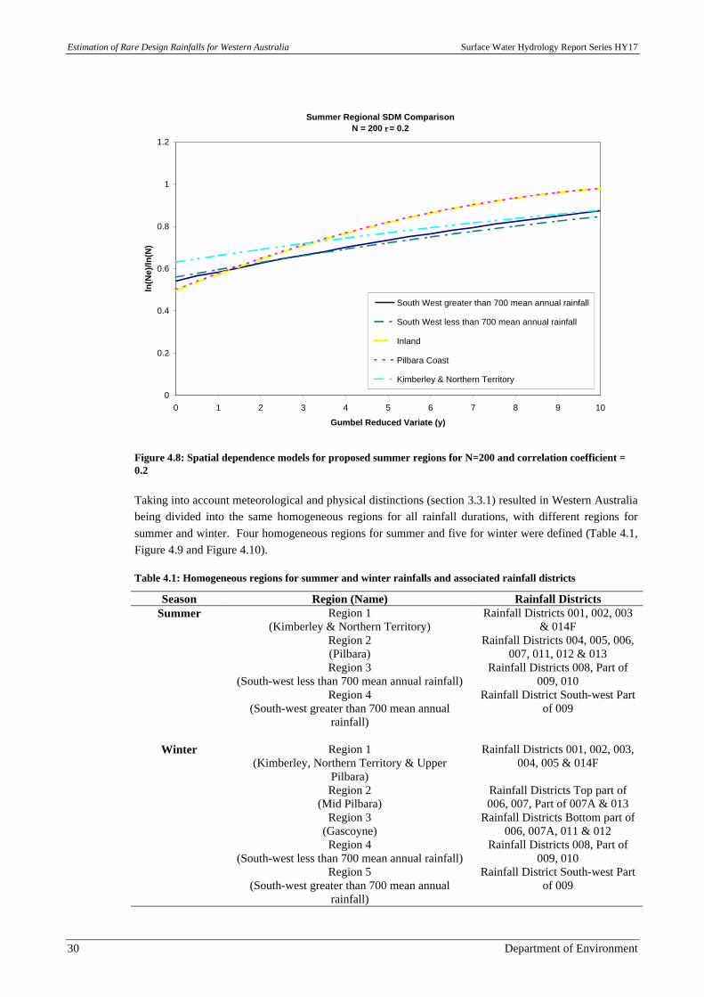
Estimation of Rare Design Rainfalls for Western Australia Surface Water Hydrology Report Series HY17
30 Department of Environment
Summer Regional SDM ComparisonN = 200 ρ= 0.2
0
0.2
0.4
0.6
0.8
1
1.2
0 1 2 3 4 5 6 7 8 9 10
Gumbel Reduced Variate (y)
ln(N
e)/ln
(N)
South West greater than 700 mean annual rainfall
South West less than 700 mean annual rainfall
Inland
Pilbara Coast
Kimberley & Northern Territory
Figure 4.8: Spatial dependence models for proposed summer regions for N=200 and correlation coefficient =0.2
Taking into account meteorological and physical distinctions (section 3.3.1) resulted in Western Australiabeing divided into the same homogeneous regions for all rainfall durations, with different regions forsummer and winter. Four homogeneous regions for summer and five for winter were defined (Table 4.1,Figure 4.9 and Figure 4.10).
Table 4.1: Homogeneous regions for summer and winter rainfalls and associated rainfall districts
Season Region (Name) Rainfall DistrictsSummer Region 1
(Kimberley & Northern Territory)Rainfall Districts 001, 002, 003
& 014FRegion 2(Pilbara)
Rainfall Districts 004, 005, 006,007, 011, 012 & 013
Region 3(South-west less than 700 mean annual rainfall)
Rainfall Districts 008, Part of009, 010
Region 4(South-west greater than 700 mean annual
rainfall)
Rainfall District South-west Partof 009
Winter Region 1(Kimberley, Northern Territory & Upper
Pilbara)
Rainfall Districts 001, 002, 003,004, 005 & 014F
Region 2(Mid Pilbara)
Rainfall Districts Top part of006, 007, Part of 007A & 013
Region 3(Gascoyne)
Rainfall Districts Bottom part of006, 007A, 011 & 012
Region 4(South-west less than 700 mean annual rainfall)
Rainfall Districts 008, Part of009, 010
Region 5(South-west greater than 700 mean annual
rainfall)
Rainfall District South-west Partof 009
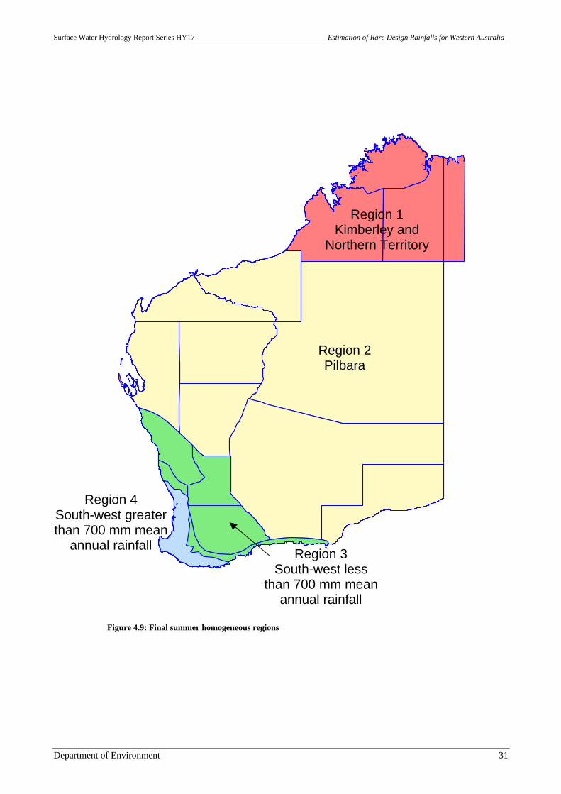
Surface Water Hydrology Report Series HY17 Estimation of Rare Design Rainfalls for Western Australia
Department of Environment 31
Region 1Kimberley and
Northern Territory
Region 2Pilbara
Region 3South-west less
than 700 mm meanannual rainfall
Region 4South-west greaterthan 700 mm mean
annual rainfall
Figure 4.9: Final summer homogeneous regions
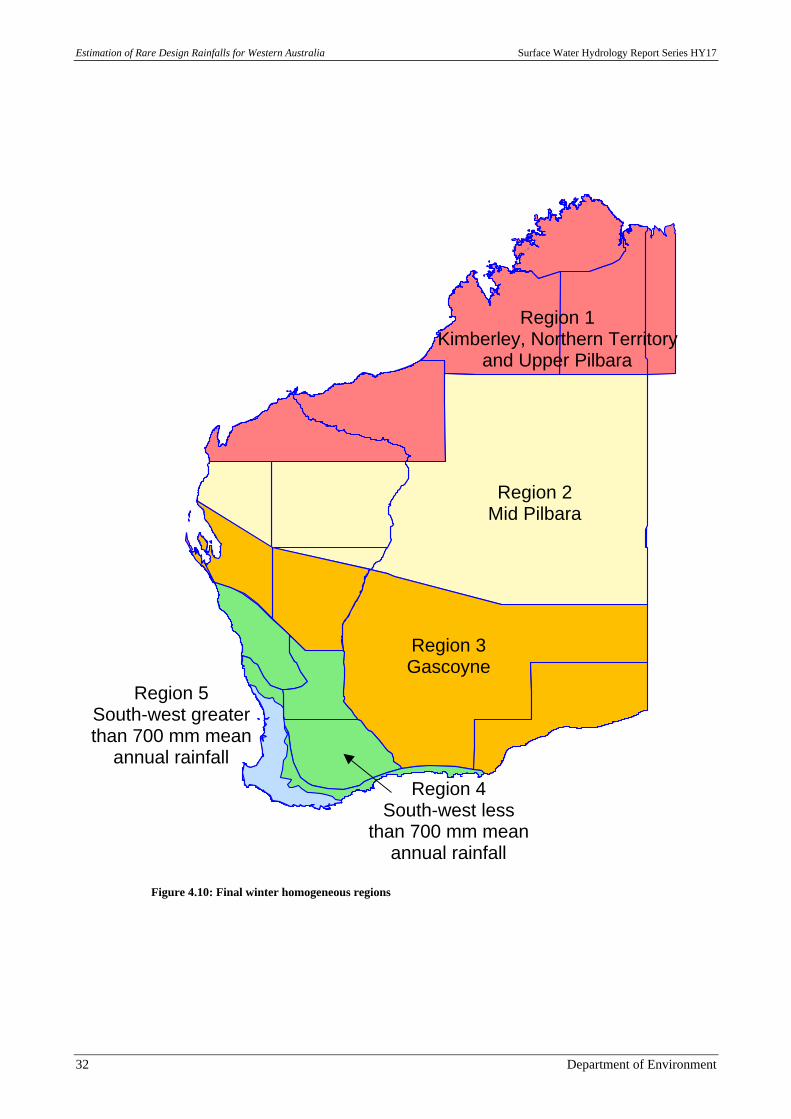
Estimation of Rare Design Rainfalls for Western Australia Surface Water Hydrology Report Series HY17
32 Department of Environment
Region 1Kimberley, Northern Territory
and Upper Pilbara
Region 2Mid Pilbara
Region 3Gascoyne
Region 4South-west less
than 700 mm meanannual rainfall
Region 5South-west greaterthan 700 mm mean
annual rainfall
Figure 4.10: Final winter homogeneous regions
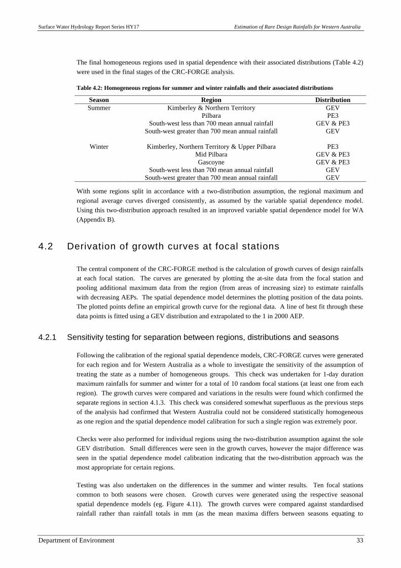
Surface Water Hydrology Report Series HY17 Estimation of Rare Design Rainfalls for Western Australia
Department of Environment 33
The final homogeneous regions used in spatial dependence with their associated distributions (Table 4.2)were used in the final stages of the CRC-FORGE analysis.
Table 4.2: Homogeneous regions for summer and winter rainfalls and their associated distributions
Season Region DistributionSummer Kimberley & Northern Territory GEV
Pilbara PE3South-west less than 700 mean annual rainfall GEV & PE3
South-west greater than 700 mean annual rainfall GEV
Winter Kimberley, Northern Territory & Upper Pilbara PE3Mid Pilbara GEV & PE3Gascoyne GEV & PE3
South-west less than 700 mean annual rainfall GEVSouth-west greater than 700 mean annual rainfall GEV
With some regions split in accordance with a two-distribution assumption, the regional maximum andregional average curves diverged consistently, as assumed by the variable spatial dependence model.Using this two-distribution approach resulted in an improved variable spatial dependence model for WA(Appendix B).
4.2 Derivation of growth curves at focal stations
The central component of the CRC-FORGE method is the calculation of growth curves of design rainfallsat each focal station. The curves are generated by plotting the at-site data from the focal station andpooling additional maximum data from the region (from areas of increasing size) to estimate rainfallswith decreasing AEPs. The spatial dependence model determines the plotting position of the data points.The plotted points define an empirical growth curve for the regional data. A line of best fit through thesedata points is fitted using a GEV distribution and extrapolated to the 1 in 2000 AEP.
4.2.1 Sensitivity testing for separation between regions, distributions and seasons
Following the calibration of the regional spatial dependence models, CRC-FORGE curves were generatedfor each region and for Western Australia as a whole to investigate the sensitivity of the assumption oftreating the state as a number of homogeneous groups. This check was undertaken for 1-day durationmaximum rainfalls for summer and winter for a total of 10 random focal stations (at least one from eachregion). The growth curves were compared and variations in the results were found which confirmed theseparate regions in section 4.1.3. This check was considered somewhat superfluous as the previous stepsof the analysis had confirmed that Western Australia could not be considered statistically homogeneousas one region and the spatial dependence model calibration for such a single region was extremely poor.
Checks were also performed for individual regions using the two-distribution assumption against the soleGEV distribution. Small differences were seen in the growth curves, however the major difference wasseen in the spatial dependence model calibration indicating that the two-distribution approach was themost appropriate for certain regions.
Testing was also undertaken on the differences in the summer and winter results. Ten focal stationscommon to both seasons were chosen. Growth curves were generated using the respective seasonalspatial dependence models (eg. Figure 4.11). The growth curves were compared against standardisedrainfall rather than rainfall totals in mm (as the mean maxima differs between seasons equating to
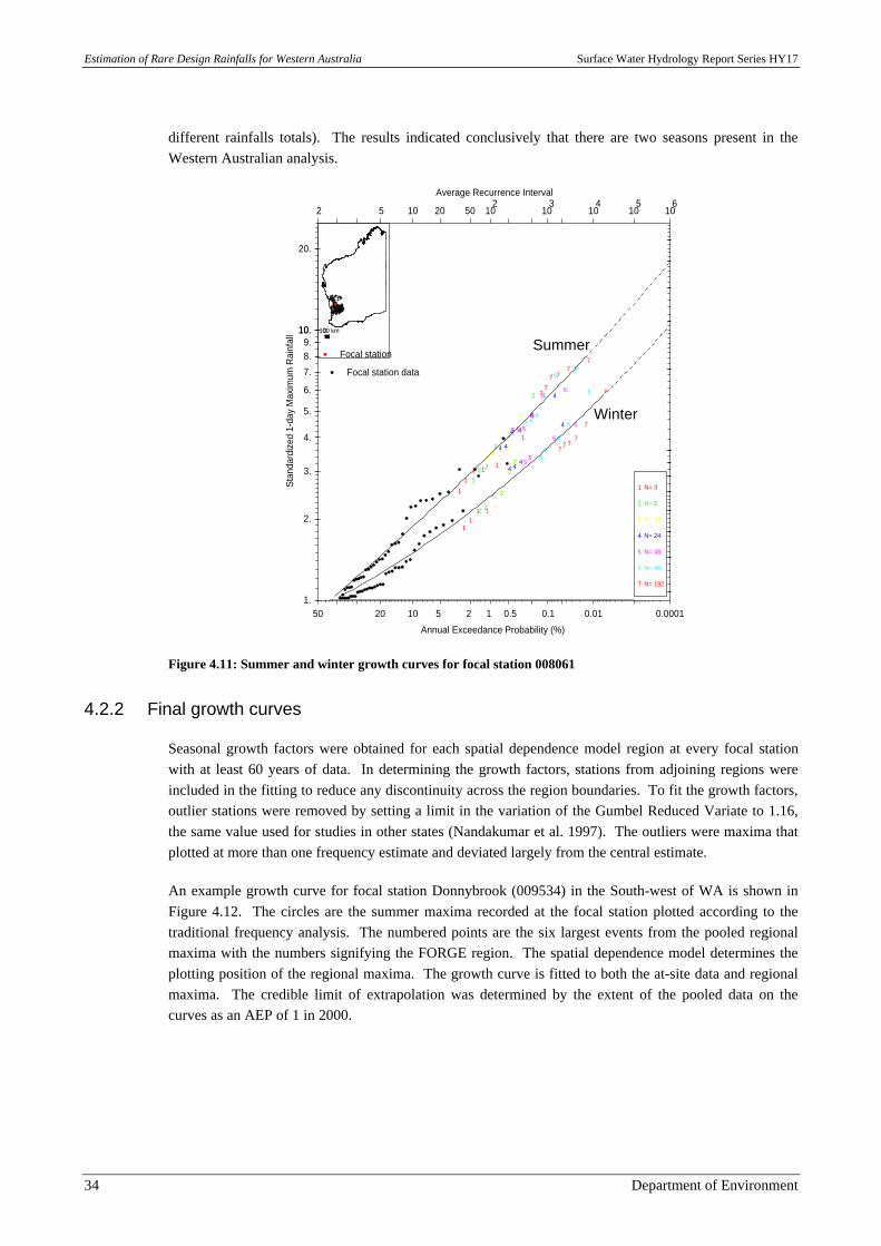
Estimation of Rare Design Rainfalls for Western Australia Surface Water Hydrology Report Series HY17
34 Department of Environment
different rainfalls totals). The results indicated conclusively that there are two seasons present in theWestern Australian analysis.
111
1
2
22
22
33
3
3
4
444
5
5
55
6
6
6
66
7
7
777
7
1 N= 3
2 N= 6
3 N= 12
4 N= 24
5 N= 48
6 N= 96
7 N= 192
100 km
Focal station
Focal station data
50
2
20
5
10
10
5
20
2
50
1
102
0.5 0.1
103
0.01
104
105
0.0001
106
Average Recurrence Interval
Annual Exceedance Probability (%)
1.
2.
3.
4.
5.
6.
7.
8. 9.
10. 10.
20.
Sta
ndar
dize
d 1-
day
Max
imum
Rai
nfal
l
30.
40.
50.
60.
70.
80. 90. 100. 100.
200.
300.
400.
500.
600.
Focal Station: 008061
1
111
1
1
2
2
2
22
2
3
3
3333
4
4
44
44
55
5
555
66
6
666
77
77
77
1 N= 3
2 N= 6
3 N= 12
4 N= 24
5 N= 48
6 N= 96
7 N= 192
0100 km
Focal station
Focal station data
Summer
Winter
Figure 4.11: Summer and winter growth curves for focal station 008061
4.2.2 Final growth curves
Seasonal growth factors were obtained for each spatial dependence model region at every focal stationwith at least 60 years of data. In determining the growth factors, stations from adjoining regions wereincluded in the fitting to reduce any discontinuity across the region boundaries. To fit the growth factors,outlier stations were removed by setting a limit in the variation of the Gumbel Reduced Variate to 1.16,the same value used for studies in other states (Nandakumar et al. 1997). The outliers were maxima thatplotted at more than one frequency estimate and deviated largely from the central estimate.
An example growth curve for focal station Donnybrook (009534) in the South-west of WA is shown inFigure 4.12. The circles are the summer maxima recorded at the focal station plotted according to thetraditional frequency analysis. The numbered points are the six largest events from the pooled regionalmaxima with the numbers signifying the FORGE region. The spatial dependence model determines theplotting position of the regional maxima. The growth curve is fitted to both the at-site data and regionalmaxima. The credible limit of extrapolation was determined by the extent of the pooled data on thecurves as an AEP of 1 in 2000.
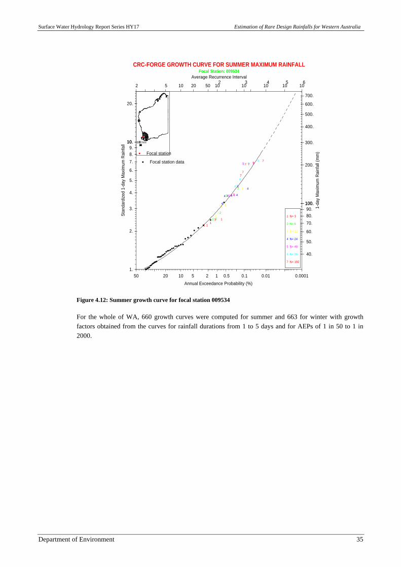
Surface Water Hydrology Report Series HY17 Estimation of Rare Design Rainfalls for Western Australia
Department of Environment 35
50
2
20
5
10
10
5
20
2
50
1
102
0.5 0.1
103
0.01
104
105
0.0001
106
Average Recurrence Interval
Annual Exceedance Probability (%)
1.
2.
3.
4.
5.
6.
7.
8. 9.
10. 10.
20.
Sta
ndar
dize
d 1-
day
Max
imum
Rai
nfal
l
40.
50.
60.
70.
80. 90. 100. 100.
200.
300.
400.
500.
600.
700.
1-da
y M
axim
um R
ainf
all (
mm
)
CRC-FORGE GROWTH CURVE FOR SUMMER MAXIMUM RAINFALLFocal Station: 009534
1
111
11
2
2
2
222
3
3
33
33
4
4444
4
55
5
555
666
6
66
7777
77
1 N= 3
2 N= 6
3 N= 12
4 N= 24
5 N= 48
6 N= 96
7 N= 192
0100 km
Focal station
Focal station data
Figure 4.12: Summer growth curve for focal station 009534
For the whole of WA, 660 growth curves were computed for summer and 663 for winter with growthfactors obtained from the curves for rainfall durations from 1 to 5 days and for AEPs of 1 in 50 to 1 in2000.
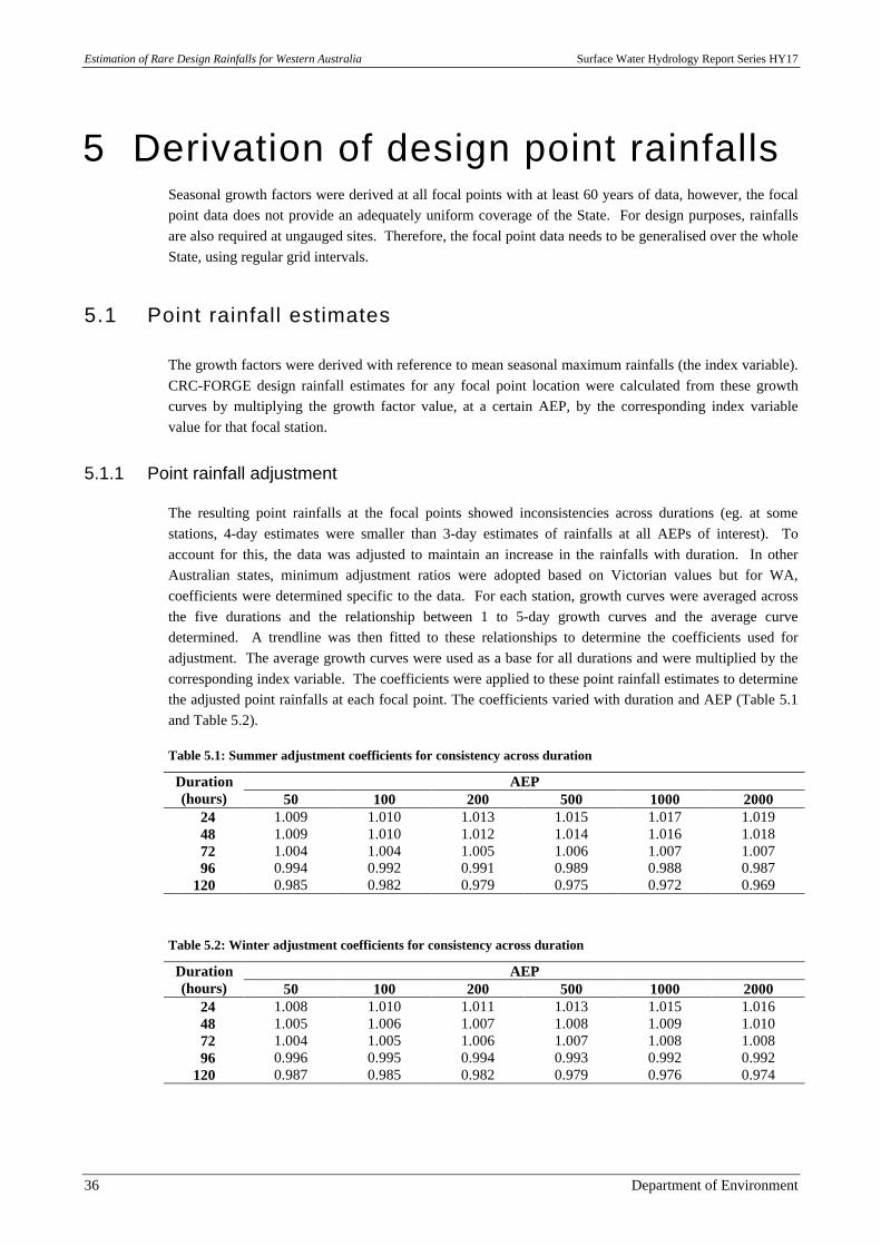
Estimation of Rare Design Rainfalls for Western Australia Surface Water Hydrology Report Series HY17
36 Department of Environment
5 Derivation of design point rainfallsSeasonal growth factors were derived at all focal points with at least 60 years of data, however, the focalpoint data does not provide an adequately uniform coverage of the State. For design purposes, rainfallsare also required at ungauged sites. Therefore, the focal point data needs to be generalised over the wholeState, using regular grid intervals.
5.1 Point rainfall estimates
The growth factors were derived with reference to mean seasonal maximum rainfalls (the index variable).CRC-FORGE design rainfall estimates for any focal point location were calculated from these growthcurves by multiplying the growth factor value, at a certain AEP, by the corresponding index variablevalue for that focal station.
5.1.1 Point rainfall adjustment
The resulting point rainfalls at the focal points showed inconsistencies across durations (eg. at somestations, 4-day estimates were smaller than 3-day estimates of rainfalls at all AEPs of interest). Toaccount for this, the data was adjusted to maintain an increase in the rainfalls with duration. In otherAustralian states, minimum adjustment ratios were adopted based on Victorian values but for WA,coefficients were determined specific to the data. For each station, growth curves were averaged acrossthe five durations and the relationship between 1 to 5-day growth curves and the average curvedetermined. A trendline was then fitted to these relationships to determine the coefficients used foradjustment. The average growth curves were used as a base for all durations and were multiplied by thecorresponding index variable. The coefficients were applied to these point rainfall estimates to determinethe adjusted point rainfalls at each focal point. The coefficients varied with duration and AEP (Table 5.1and Table 5.2).
Table 5.1: Summer adjustment coefficients for consistency across duration
AEPDuration(hours) 50 100 200 500 1000 2000
24 1.009 1.010 1.013 1.015 1.017 1.019 48 1.009 1.010 1.012 1.014 1.016 1.018 72 1.004 1.004 1.005 1.006 1.007 1.007 96 0.994 0.992 0.991 0.989 0.988 0.987120 0.985 0.982 0.979 0.975 0.972 0.969
Table 5.2: Winter adjustment coefficients for consistency across duration
AEPDuration(hours) 50 100 200 500 1000 2000
24 1.008 1.010 1.011 1.013 1.015 1.016 48 1.005 1.006 1.007 1.008 1.009 1.010 72 1.004 1.005 1.006 1.007 1.008 1.008 96 0.996 0.995 0.994 0.993 0.992 0.992120 0.987 0.985 0.982 0.979 0.976 0.974
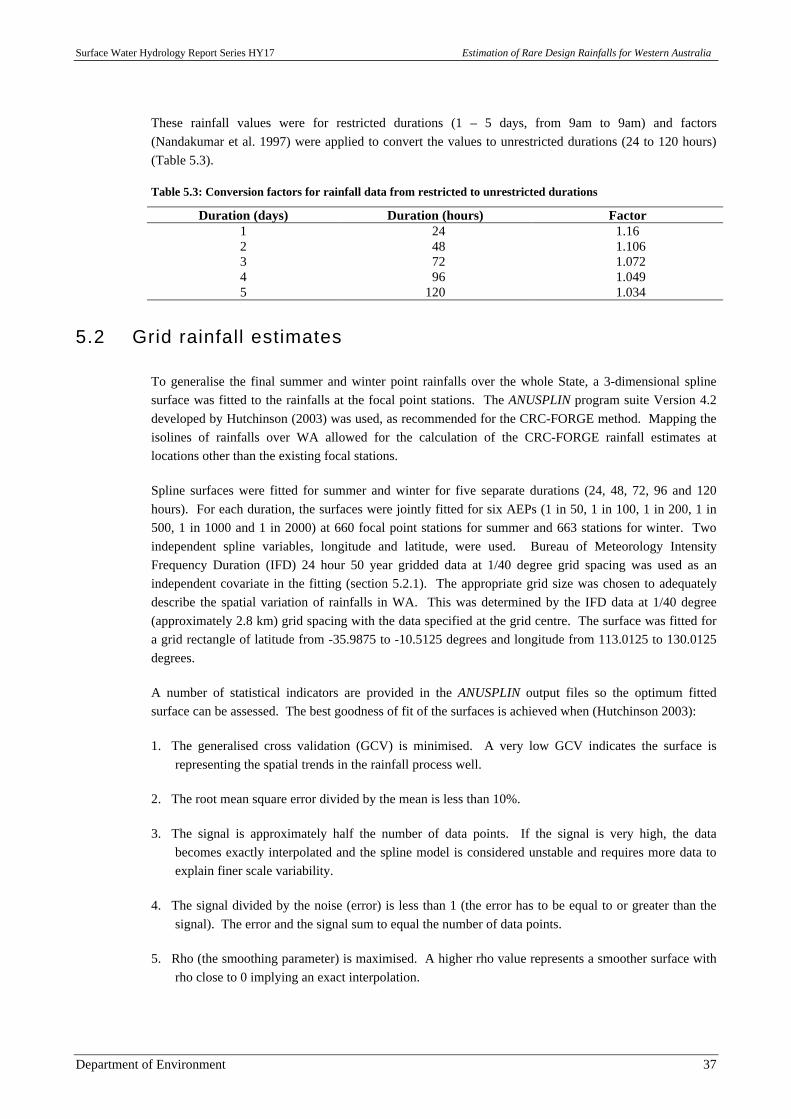
Surface Water Hydrology Report Series HY17 Estimation of Rare Design Rainfalls for Western Australia
Department of Environment 37
These rainfall values were for restricted durations (1 – 5 days, from 9am to 9am) and factors(Nandakumar et al. 1997) were applied to convert the values to unrestricted durations (24 to 120 hours)(Table 5.3).
Table 5.3: Conversion factors for rainfall data from restricted to unrestricted durations
Duration (days) Duration (hours) Factor1 24 1.162 48 1.1063 72 1.0724 96 1.0495 120 1.034
5.2 Grid rainfall estimates
To generalise the final summer and winter point rainfalls over the whole State, a 3-dimensional splinesurface was fitted to the rainfalls at the focal point stations. The ANUSPLIN program suite Version 4.2developed by Hutchinson (2003) was used, as recommended for the CRC-FORGE method. Mapping theisolines of rainfalls over WA allowed for the calculation of the CRC-FORGE rainfall estimates atlocations other than the existing focal stations.
Spline surfaces were fitted for summer and winter for five separate durations (24, 48, 72, 96 and 120hours). For each duration, the surfaces were jointly fitted for six AEPs (1 in 50, 1 in 100, 1 in 200, 1 in500, 1 in 1000 and 1 in 2000) at 660 focal point stations for summer and 663 stations for winter. Twoindependent spline variables, longitude and latitude, were used. Bureau of Meteorology IntensityFrequency Duration (IFD) 24 hour 50 year gridded data at 1/40 degree grid spacing was used as anindependent covariate in the fitting (section 5.2.1). The appropriate grid size was chosen to adequatelydescribe the spatial variation of rainfalls in WA. This was determined by the IFD data at 1/40 degree(approximately 2.8 km) grid spacing with the data specified at the grid centre. The surface was fitted fora grid rectangle of latitude from -35.9875 to -10.5125 degrees and longitude from 113.0125 to 130.0125degrees.
A number of statistical indicators are provided in the ANUSPLIN output files so the optimum fittedsurface can be assessed. The best goodness of fit of the surfaces is achieved when (Hutchinson 2003):
1. The generalised cross validation (GCV) is minimised. A very low GCV indicates the surface isrepresenting the spatial trends in the rainfall process well.
2. The root mean square error divided by the mean is less than 10%.
3. The signal is approximately half the number of data points. If the signal is very high, the databecomes exactly interpolated and the spline model is considered unstable and requires more data toexplain finer scale variability.
4. The signal divided by the noise (error) is less than 1 (the error has to be equal to or greater than thesignal). The error and the signal sum to equal the number of data points.
5. Rho (the smoothing parameter) is maximised. A higher rho value represents a smoother surface withrho close to 0 implying an exact interpolation.
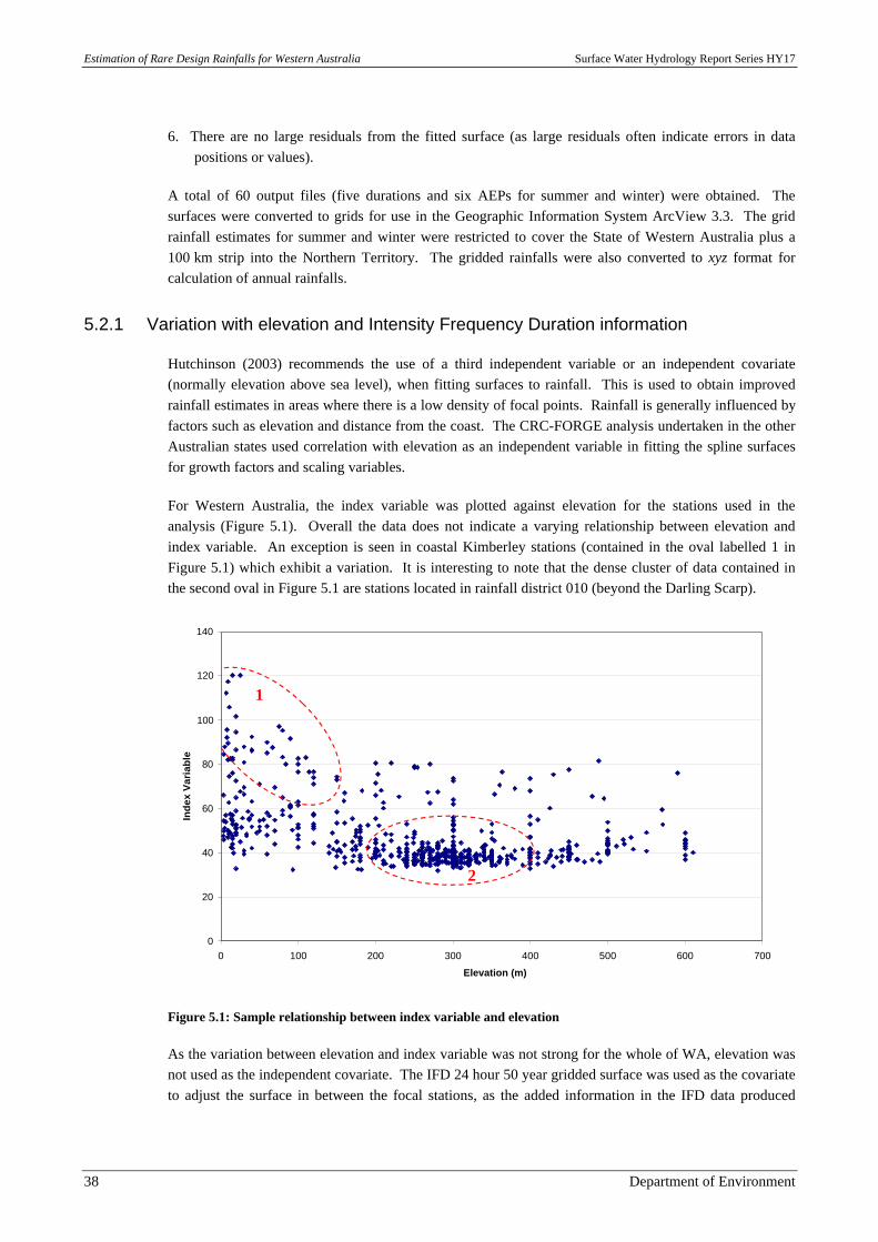
Estimation of Rare Design Rainfalls for Western Australia Surface Water Hydrology Report Series HY17
38 Department of Environment
6. There are no large residuals from the fitted surface (as large residuals often indicate errors in datapositions or values).
A total of 60 output files (five durations and six AEPs for summer and winter) were obtained. Thesurfaces were converted to grids for use in the Geographic Information System ArcView 3.3. The gridrainfall estimates for summer and winter were restricted to cover the State of Western Australia plus a100 km strip into the Northern Territory. The gridded rainfalls were also converted to xyz format forcalculation of annual rainfalls.
5.2.1 Variation with elevation and Intensity Frequency Duration information
Hutchinson (2003) recommends the use of a third independent variable or an independent covariate(normally elevation above sea level), when fitting surfaces to rainfall. This is used to obtain improvedrainfall estimates in areas where there is a low density of focal points. Rainfall is generally influenced byfactors such as elevation and distance from the coast. The CRC-FORGE analysis undertaken in the otherAustralian states used correlation with elevation as an independent variable in fitting the spline surfacesfor growth factors and scaling variables.
For Western Australia, the index variable was plotted against elevation for the stations used in theanalysis (Figure 5.1). Overall the data does not indicate a varying relationship between elevation andindex variable. An exception is seen in coastal Kimberley stations (contained in the oval labelled 1 inFigure 5.1) which exhibit a variation. It is interesting to note that the dense cluster of data contained inthe second oval in Figure 5.1 are stations located in rainfall district 010 (beyond the Darling Scarp).
0
20
40
60
80
100
120
140
0 100 200 300 400 500 600 700
Elevation (m)
Ind
ex V
aria
ble
120
100
Figure 5.1: Sample relationship between index variable and elevation
As the variation between elevation and index variable was not strong for the whole of WA, elevation wasnot used as the independent covariate. The IFD 24 hour 50 year gridded surface was used as the covariateto adjust the surface in between the focal stations, as the added information in the IFD data produced
1
2
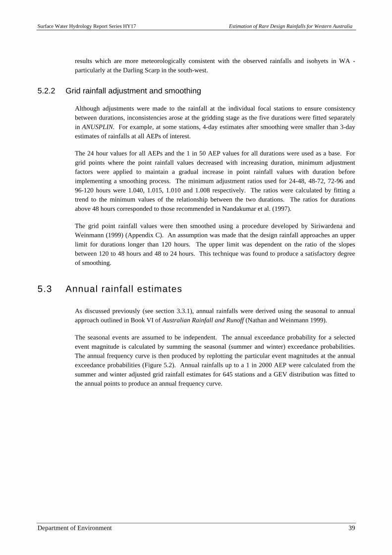
Surface Water Hydrology Report Series HY17 Estimation of Rare Design Rainfalls for Western Australia
Department of Environment 39
results which are more meteorologically consistent with the observed rainfalls and isohyets in WA -particularly at the Darling Scarp in the south-west.
5.2.2 Grid rainfall adjustment and smoothing
Although adjustments were made to the rainfall at the individual focal stations to ensure consistencybetween durations, inconsistencies arose at the gridding stage as the five durations were fitted separatelyin ANUSPLIN. For example, at some stations, 4-day estimates after smoothing were smaller than 3-dayestimates of rainfalls at all AEPs of interest.
The 24 hour values for all AEPs and the 1 in 50 AEP values for all durations were used as a base. Forgrid points where the point rainfall values decreased with increasing duration, minimum adjustmentfactors were applied to maintain a gradual increase in point rainfall values with duration beforeimplementing a smoothing process. The minimum adjustment ratios used for 24-48, 48-72, 72-96 and96-120 hours were 1.040, 1.015, 1.010 and 1.008 respectively. The ratios were calculated by fitting atrend to the minimum values of the relationship between the two durations. The ratios for durationsabove 48 hours corresponded to those recommended in Nandakumar et al. (1997).
The grid point rainfall values were then smoothed using a procedure developed by Siriwardena andWeinmann (1999) (Appendix C). An assumption was made that the design rainfall approaches an upperlimit for durations longer than 120 hours. The upper limit was dependent on the ratio of the slopesbetween 120 to 48 hours and 48 to 24 hours. This technique was found to produce a satisfactory degreeof smoothing.
5.3 Annual rainfall estimates
As discussed previously (see section 3.3.1), annual rainfalls were derived using the seasonal to annualapproach outlined in Book VI of Australian Rainfall and Runoff (Nathan and Weinmann 1999).
The seasonal events are assumed to be independent. The annual exceedance probability for a selectedevent magnitude is calculated by summing the seasonal (summer and winter) exceedance probabilities.The annual frequency curve is then produced by replotting the particular event magnitudes at the annualexceedance probabilities (Figure 5.2). Annual rainfalls up to a 1 in 2000 AEP were calculated from thesummer and winter adjusted grid rainfall estimates for 645 stations and a GEV distribution was fitted tothe annual points to produce an annual frequency curve.
Estimation of Rare Design Rainfalls for Western Australia Surface Water Hydrology Report Series HY17
40 Department of Environment
100
7080
200
300
400
500
600
700800900
Rai
nfal
l (m
m)
0.02 0.01 10-3 10-4
A EP
CRCFORGE 1-day Rainfal l Frequency Curve For Stat ion: 006008
Sum mer
W i nter
A nnual
Figure 5.2: Calculation of annual design rainfalls from seasonal frequency curves
The annual design rainfalls were also adjusted and smoothed using the same minimum adjustment ratiosas for summer and winter of 1.040, 1.015, 1.010 and 1.008 for 24-48, 48-72, 72-96 and 96-120 hoursrespectively.
5.4 Final design point rainfalls
The result of applying the CRC-FORGE methodology to WA is final design point rainfalls for annual,summer and winter for durations of 24, 48, 72, 96 and 120 hours and AEPs of 1 in 50, 1 in 100, 1 in 200,1 in 500, 1 in 1000 and 1 in 2000 for every 1/40 degree grid spacing across WA.
5.5 Comparison of CRC-FORGE rainfalls with ARR87 data andat-site estimates
Comparisons were made between the seasonal final CRC-FORGE design rainfalls and at-site frequencyestimates, and the annual final CRC-FORGE design rainfalls and Australian Rainfall and Runoff(ARR87) (Canterford et al, 1998) estimates for AEPs of 1 in 50 and 1 in 100 for different duration eventsat 23 locations distributed over the whole State. These stations included many of the most extremerainfall events that have occurred in Western Australia (Appendix D).
The seasonal values obtained from CRC-FORGE and the at-site frequency analysis could not be directlycompared as different distributions were used, however it was reasonable to expect the results to besimilar as the bottom end of the CRC-FORGE growth curves (up to 1 in 100 AEP) were determined using
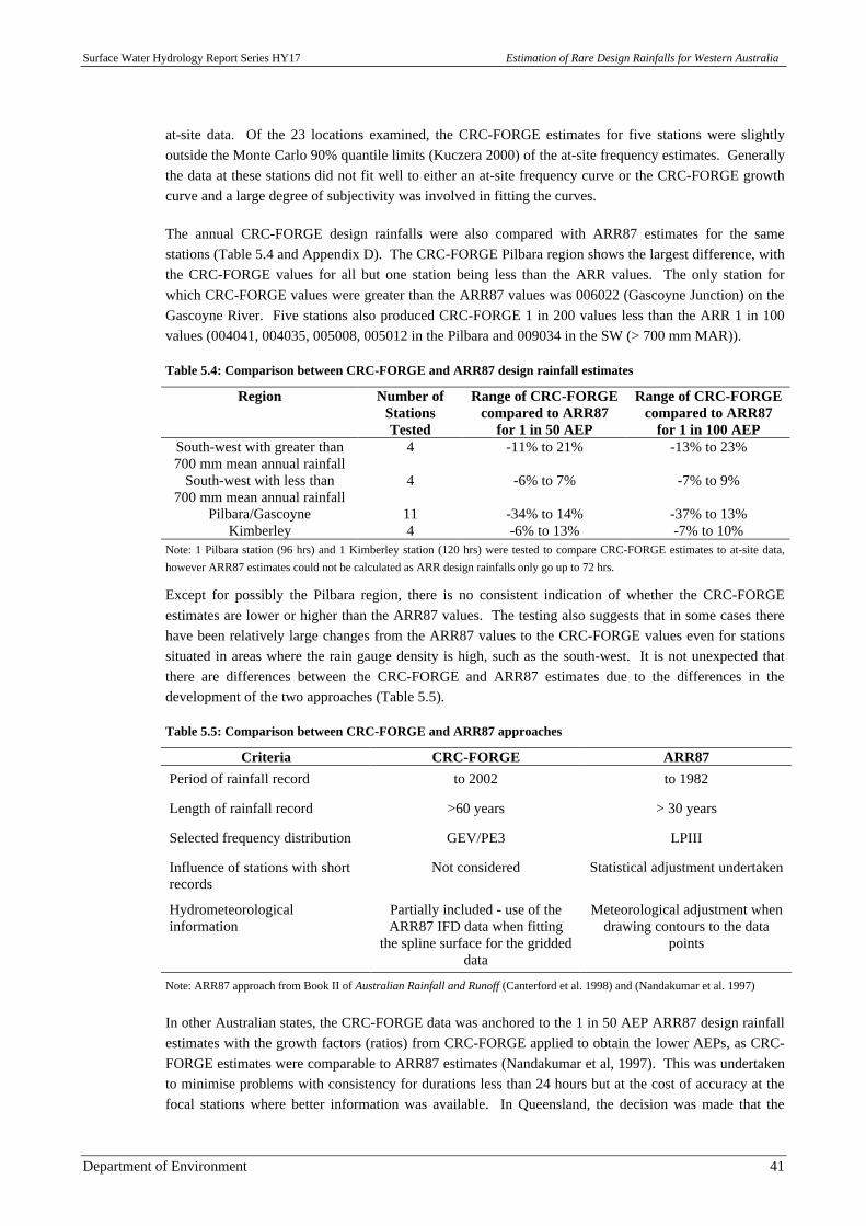
Surface Water Hydrology Report Series HY17 Estimation of Rare Design Rainfalls for Western Australia
Department of Environment 41
at-site data. Of the 23 locations examined, the CRC-FORGE estimates for five stations were slightlyoutside the Monte Carlo 90% quantile limits (Kuczera 2000) of the at-site frequency estimates. Generallythe data at these stations did not fit well to either an at-site frequency curve or the CRC-FORGE growthcurve and a large degree of subjectivity was involved in fitting the curves.
The annual CRC-FORGE design rainfalls were also compared with ARR87 estimates for the samestations (Table 5.4 and Appendix D). The CRC-FORGE Pilbara region shows the largest difference, withthe CRC-FORGE values for all but one station being less than the ARR values. The only station forwhich CRC-FORGE values were greater than the ARR87 values was 006022 (Gascoyne Junction) on theGascoyne River. Five stations also produced CRC-FORGE 1 in 200 values less than the ARR 1 in 100values (004041, 004035, 005008, 005012 in the Pilbara and 009034 in the SW (> 700 mm MAR)).
Table 5.4: Comparison between CRC-FORGE and ARR87 design rainfall estimates
Region Number ofStationsTested
Range of CRC-FORGEcompared to ARR87
for 1 in 50 AEP
Range of CRC-FORGEcompared to ARR87
for 1 in 100 AEPSouth-west with greater than700 mm mean annual rainfall
4 -11% to 21% -13% to 23%
South-west with less than700 mm mean annual rainfall
4 -6% to 7% -7% to 9%
Pilbara/Gascoyne 11 -34% to 14% -37% to 13%Kimberley 4 -6% to 13% -7% to 10%
Note: 1 Pilbara station (96 hrs) and 1 Kimberley station (120 hrs) were tested to compare CRC-FORGE estimates to at-site data,however ARR87 estimates could not be calculated as ARR design rainfalls only go up to 72 hrs.
Except for possibly the Pilbara region, there is no consistent indication of whether the CRC-FORGEestimates are lower or higher than the ARR87 values. The testing also suggests that in some cases therehave been relatively large changes from the ARR87 values to the CRC-FORGE values even for stationssituated in areas where the rain gauge density is high, such as the south-west. It is not unexpected thatthere are differences between the CRC-FORGE and ARR87 estimates due to the differences in thedevelopment of the two approaches (Table 5.5).
Table 5.5: Comparison between CRC-FORGE and ARR87 approaches
Criteria CRC-FORGE ARR87Period of rainfall record to 2002 to 1982
Length of rainfall record >60 years > 30 years
Selected frequency distribution GEV/PE3 LPIII
Influence of stations with shortrecords
Not considered Statistical adjustment undertaken
Hydrometeorologicalinformation
Partially included - use of theARR87 IFD data when fitting
the spline surface for the griddeddata
Meteorological adjustment whendrawing contours to the data
points
Note: ARR87 approach from Book II of Australian Rainfall and Runoff (Canterford et al. 1998) and (Nandakumar et al. 1997)
In other Australian states, the CRC-FORGE data was anchored to the 1 in 50 AEP ARR87 design rainfallestimates with the growth factors (ratios) from CRC-FORGE applied to obtain the lower AEPs, as CRC-FORGE estimates were comparable to ARR87 estimates (Nandakumar et al, 1997). This was undertakento minimise problems with consistency for durations less than 24 hours but at the cost of accuracy at thefocal stations where better information was available. In Queensland, the decision was made that the
Estimation of Rare Design Rainfalls for Western Australia Surface Water Hydrology Report Series HY17
42 Department of Environment
CRC-FORGE represented the best estimates, confirmed by independent testing, as a larger data set wasused in the analysis (Hargraves in prep.).
For Western Australia, the CRC-FORGE data was not anchored to the ARR87 1 in 50 AEP estimates asthe estimates produced from the seasonal CRC-FORGE approach for all AEPs were considered to bemore appropriate for Western Australia. As discussed previously, Pearce (1998) raised the importance ofusing seasonal rainfall for WA, and as the ARR87 estimates are for annual data only, anchoring to thisvalue would reduce the accuracy of the seasonal estimates. The additional 20 years of data used for theCRC-FORGE approach compared to the ARR87 approach is also considered to have increased theaccuracy of the CRC-FORGE estimates.
Surface Water Hydrology Report Series HY17 Estimation of Rare Design Rainfalls for Western Australia
Department of Environment 43
6 CRC-FORGE areal reductionfactors
6.1 Introduction
The final CRC-FORGE design rainfall estimates are provided as point rainfall intensities at focal stationsand grid intervals across the State. However, most design rainfall estimates are required for catchmentsof significant size and therefore require an estimate of the areal average rainfall over the catchment, ratherthan at a point. An Areal Reduction Factor (ARF) is the ratio of areal average rainfall to point rainfall forthe same duration and annual exceedance probability. Conceptually, this factor represents the fact thatlarger catchments are less likely to experience high intensity storms over the whole catchment.
Current practice for Western Australia is to apply areal reduction factors estimated from the arealreduction curves provided in Book II of Australian Rainfall and Runoff (Canterford et al, 1998). Theseare based on data from the United States, with a set of curves from a 1980 study of data from Chicagorecommended for the coastal region and design values from a 1984 study of data from Arizonarecommended for the arid region of Australia. These curves are only applicable for AEPs greater than 1in 100 and durations less than or equal to 24 hours. The appropriateness of these factors to Australianconditions has been addressed in other CRC-CH studies conducted in other Australian states and theresults produced highlight the inadequacy of those currently recommended (Siriwardena and Weinmann1996).
Areal reduction factors were calculated for Western Australia based on the analysis of daily rainfall datafor the whole State using a modified version of Bell’s method (Siriwardena and Weinmann, 1996), whichwas an additional project to CRC-FORGE, implemented by the CRC-CH. Values were determined fordurations from 24 to 120 hours for a range of hypothetical circular catchments ranging from 50 to8000 km2 in area. Regional non-linear relationships were then derived from the mean values for eacharea, duration and AEP. These ARF design curves were produced on an annual, summer and winterbasis.
6.2 Disaggregation of rainfall data for ARF analysis
The calculation of areal reduction factors requires a continuous time series of daily rainfall data. TheCRC-FORGE method only requires annual or seasonal maxima and hence any accumulated rainfall wasonly disaggregated if it was required to determine the maxima. Consequently, all the remainingaccumulated totals were disaggregated to daily totals to compute the areal reduction factors. Thedisaggregation of these values was automated using a program developed by the CRC-CH whichdisaggregates the accumulated data based upon temporal patterns of nearby rainfall stations for the sameperiod (Nandakumar et al, 1997).
Estimation of Rare Design Rainfalls for Western Australia Surface Water Hydrology Report Series HY17
44 Department of Environment
6.3 Generation of hypothetical catchments
Hypothetical circular catchments were generated for Western Australia for each of the eight catchmentareas analysed (50, 125, 250, 500, 1000, 2000, 4000 and 8000 km2). The selection of the catchments wassubject to constraints to ensure the accuracy and independence of the estimated ARF values. Theminimum number of stations per catchment was set at three stations, plus an additional station for eachadditional 500 km2 of catchment area. Queensland’s Department of Natural Resources (Hargraves inprep) developed an ArcView Avenue script to automate this procedure with an additional constraint of themaximum proportion of stations allowed to be included in overlapping catchments set to 30%. Rainfallstations with greater than 30 years of data were used in the analysis.
Due to the sparse distribution of rainfall gauges in the arid, less populated regions of Western Australia,there was a significant lack of hypothetical catchments generated beyond the South-west region (Figure6.1). Figure 6.1 is indicative of the catchments generated for analysis for all catchment sizes with the vastmajority of sample catchments weighted to the South-west region. Decreasing the constraints of theminimum number of stations per catchment and the number of years of data at each station did result inmarginally more catchments being selected in the northern regions. However, the minimal gain incoverage was considered a significant tradeoff with the increasing uncertainty introduced by using shorterrecord lengths and fewer stations to calculate the mean values.
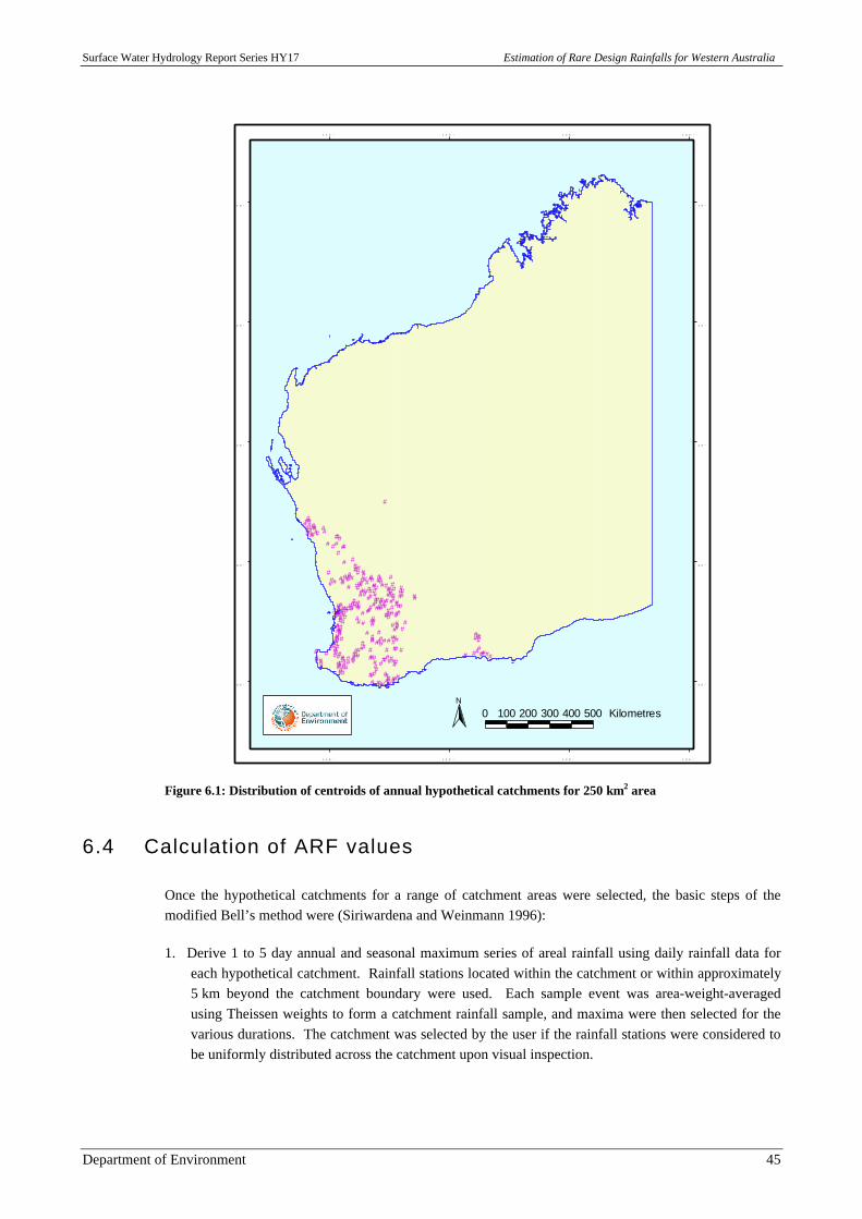
Surface Water Hydrology Report Series HY17 Estimation of Rare Design Rainfalls for Western Australia
Department of Environment 45
#
####### ##### ####### #### ## ##
### #### ### ## # ### ## ## # ## # # ### # ### ## # ## ## # ## ## # ### ## ## ## # #### ## ### ## ## ## ### ### ### ### ## ### ## ## # # #### # # ### #### ##### # ### ## # #### # ## ## # ### #### #### ## ## # ## # #### ## ##### ## # ## ### # ## ## ## # # ## ## ### ## ## ### # ### ## ## # ### ### ### ### ## ## # # ## # # ## # ## #### # # ## ### ### # ## ## # #### ## ## # #### # ## ## ## ######## ###3 5 ° 3 5 °
3 0 ° 3 0 °
2 5 ° 2 5 °
2 0 ° 2 0 °
1 5 ° 1 5 °
1 1 5 °
1 1 5 °
1 2 0 °
1 2 0 °
1 2 5 °
1 2 5 °
1 3 0 °
1 3 0 °
0 100 200 300 400 500 KilometresN
Figure 6.1: Distribution of centroids of annual hypothetical catchments for 250 km2 area
6.4 Calculation of ARF values
Once the hypothetical catchments for a range of catchment areas were selected, the basic steps of themodified Bell’s method were (Siriwardena and Weinmann 1996):
1. Derive 1 to 5 day annual and seasonal maximum series of areal rainfall using daily rainfall data foreach hypothetical catchment. Rainfall stations located within the catchment or within approximately5 km beyond the catchment boundary were used. Each sample event was area-weight-averagedusing Theissen weights to form a catchment rainfall sample, and maxima were then selected for thevarious durations. The catchment was selected by the user if the rainfall stations were considered tobe uniformly distributed across the catchment upon visual inspection.
Estimation of Rare Design Rainfalls for Western Australia Surface Water Hydrology Report Series HY17
46 Department of Environment
2. Fit a Generalised Extreme Value (GEV) probability distribution to the annual and seasonal series ofareal and point rainfalls and estimate rainfall quantiles (for AEPs from 1 in 2 to 1 in 100).Constraints on the record length were imposed to ensure accuracy of the parameters of the GEVdistribution and the areal estimates, with estimates only calculated if the series contained greater than30 years of data and, for the 1 in 100 AEP estimate, greater than 50 years of data.
3. Calculate values of fixed area ARFs as a ratio between the weighted areal and weighted mean pointrainfall estimates for each AEP.
4. Fit a generalised non-linear relationship to the mean values for each duration, area and AEP takinginto account regional variability in ARFs.
The first three points of the process, including calculating the areal reduction factors, were automatedusing CRC programs (Siriwardena and Weinmann 1996).
6.5 Regional variability in ARFs
Due to the sparse distribution of rainfall gauges beyond the South-west region, it was not possible toidentify the presence, or absence, of statistical regions dependent on spatial variation of ARFs. Thereforedemarcation of initial regional boundaries was determined on the basis of topographical andmeteorological considerations. It was concluded to use the regions identified in the homogeneity analysis(Figure 4.9 and Figure 4.10) as initial ARF regions. These regions were then statistically tested to seewhether the regional mean values of ARFs were significantly different enough to calculate the final ARFsby regions.
For annual, summer and winter for each region, the number of valid catchment samples for a 24 hourduration, 0.5 (1 in 2) AEP and a 250 km2 catchment area is shown in Table 6.1. Average ARFs werederived for each region for the range of AEPs and durations. Averages were also derived for the entireState as one region.
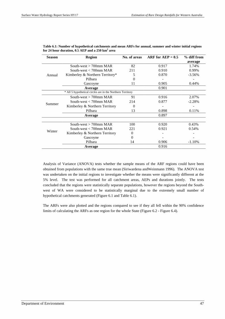
Surface Water Hydrology Report Series HY17 Estimation of Rare Design Rainfalls for Western Australia
Department of Environment 47
Table 6.1: Number of hypothetical catchments and mean ARFs for annual, summer and winter initial regionsfor 24 hour duration, 0.5 AEP and a 250 km2 area
Season Region No. of areas ARF for AEP = 0.5 % diff fromaverage
South-west > 700mm MAR 82 0.917 1.74%South-west < 700mm MAR 211 0.910 0.99%
Kimberley & Northern Territory* 5 0.870 -3.56%Pilbara 0 - -
Gascoyne 11 0.905 0.44%
Annual
Average 0.901* All 5 hypothetical circles are in the Northern Territory
South-west > 700mm MAR 91 0.916 2.07%South-west < 700mm MAR 214 0.877 -2.28%
Kimberley & Northern Territory 0 - -Pilbara 13 0.898 0.11%
Summer
Average 0.897
South-west > 700mm MAR 100 0.920 0.43%South-west < 700mm MAR 221 0.921 0.54%
Kimberley & Northern Territory 0 - -Gascoyne 0 - -
Pilbara 14 0.906 -1.10%
Winter
Average 0.916
Analysis of Variance (ANOVA) tests whether the sample means of the ARF regions could have beenobtained from populations with the same true mean (Siriwardena andWeinmann 1996). The ANOVA testwas undertaken on the initial regions to investigate whether the means were significantly different at the5% level. The test was performed for all catchment areas, AEPs and durations jointly. The testsconcluded that the regions were statistically separate populations, however the regions beyond the South-west of WA were considered to be statistically marginal due to the extremely small number ofhypothetical catchments generated (Figure 6.1 and Table 6.1).
The ARFs were also plotted and the regions compared to see if they all fell within the 90% confidencelimits of calculating the ARFs as one region for the whole State (Figure 6.2 - Figure 6.4).
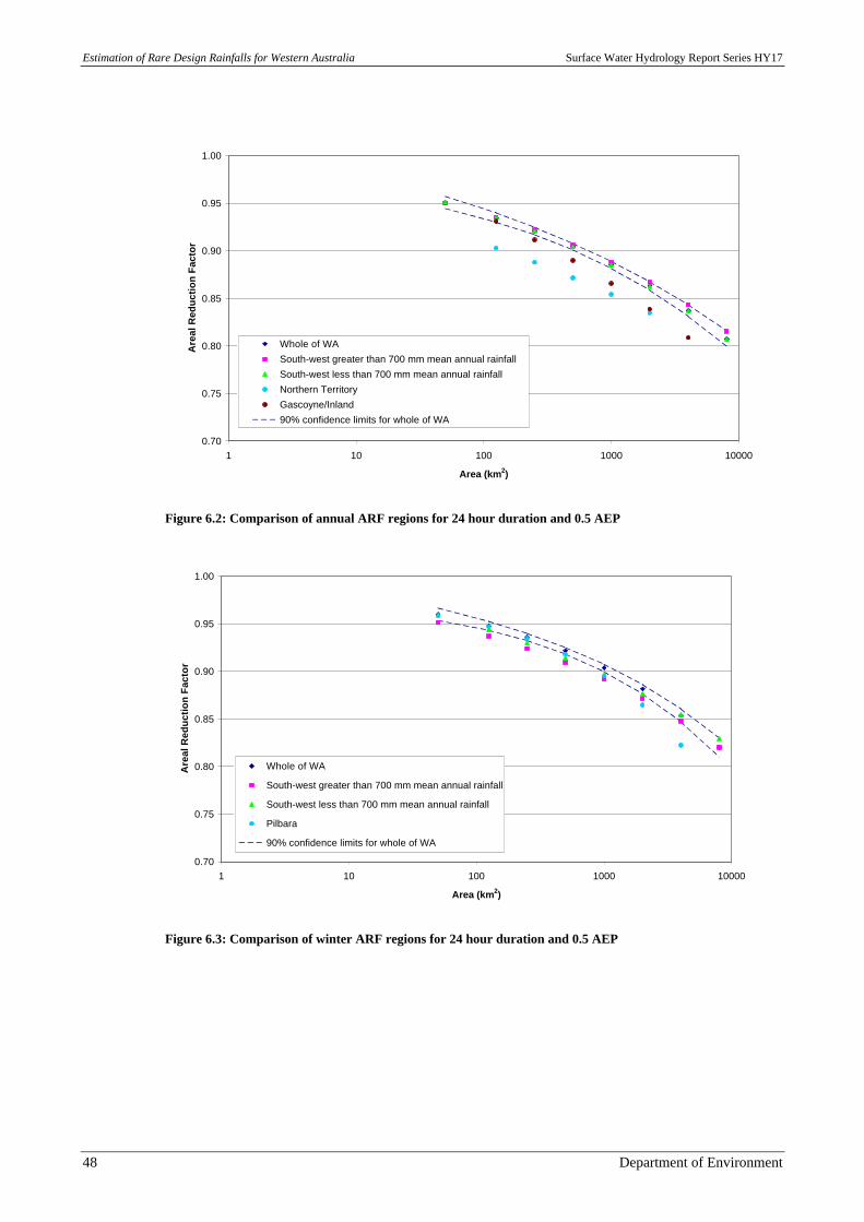
Estimation of Rare Design Rainfalls for Western Australia Surface Water Hydrology Report Series HY17
48 Department of Environment
0.70
0.75
0.80
0.85
0.90
0.95
1.00
1 10 100 1000 10000
Area (km2)
Are
al R
edu
ctio
n F
acto
r
Whole of WA
South-west greater than 700 mm mean annual rainfall
South-west less than 700 mm mean annual rainfall
Northern Territory
Gascoyne/Inland
90% confidence limits for whole of WA
Figure 6.2: Comparison of annual ARF regions for 24 hour duration and 0.5 AEP
0.70
0.75
0.80
0.85
0.90
0.95
1.00
1 10 100 1000 10000
Area (km2)
Are
al R
edu
ctio
n F
acto
r
Whole of WA
South-west greater than 700 mm mean annual rainfall
South-west less than 700 mm mean annual rainfall
Pilbara
90% confidence limits for whole of WA
Figure 6.3: Comparison of winter ARF regions for 24 hour duration and 0.5 AEP
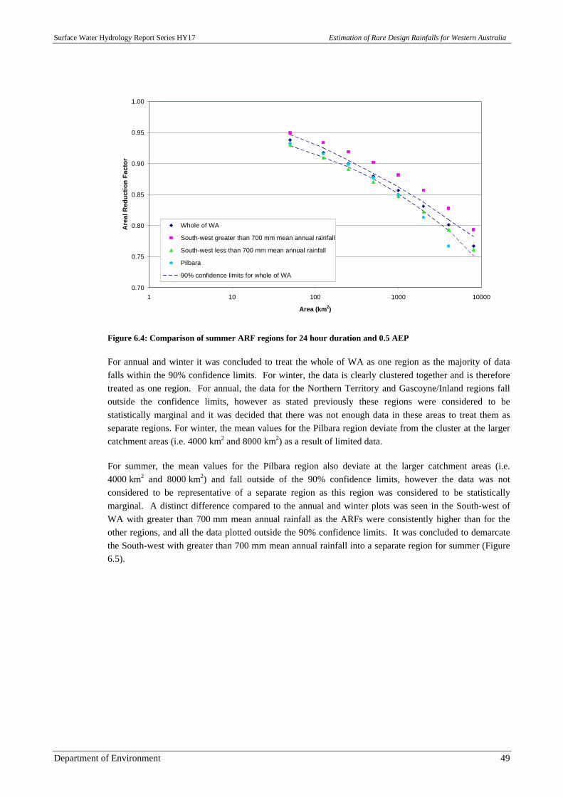
Surface Water Hydrology Report Series HY17 Estimation of Rare Design Rainfalls for Western Australia
Department of Environment 49
0.70
0.75
0.80
0.85
0.90
0.95
1.00
1 10 100 1000 10000
Area (km2)
Are
al R
edu
ctio
n F
acto
r
Whole of WA
South-west greater than 700 mm mean annual rainfall
South-west less than 700 mm mean annual rainfall
Pilbara
90% confidence limits for whole of WA
Figure 6.4: Comparison of summer ARF regions for 24 hour duration and 0.5 AEP
For annual and winter it was concluded to treat the whole of WA as one region as the majority of datafalls within the 90% confidence limits. For winter, the data is clearly clustered together and is thereforetreated as one region. For annual, the data for the Northern Territory and Gascoyne/Inland regions falloutside the confidence limits, however as stated previously these regions were considered to bestatistically marginal and it was decided that there was not enough data in these areas to treat them asseparate regions. For winter, the mean values for the Pilbara region deviate from the cluster at the largercatchment areas (i.e. 4000 km2 and 8000 km2) as a result of limited data.
For summer, the mean values for the Pilbara region also deviate at the larger catchment areas (i.e.4000 km2 and 8000 km2) and fall outside of the 90% confidence limits, however the data was notconsidered to be representative of a separate region as this region was considered to be statisticallymarginal. A distinct difference compared to the annual and winter plots was seen in the South-west ofWA with greater than 700 mm mean annual rainfall as the ARFs were consistently higher than for theother regions, and all the data plotted outside the 90% confidence limits. It was concluded to demarcatethe South-west with greater than 700 mm mean annual rainfall into a separate region for summer (Figure6.5).
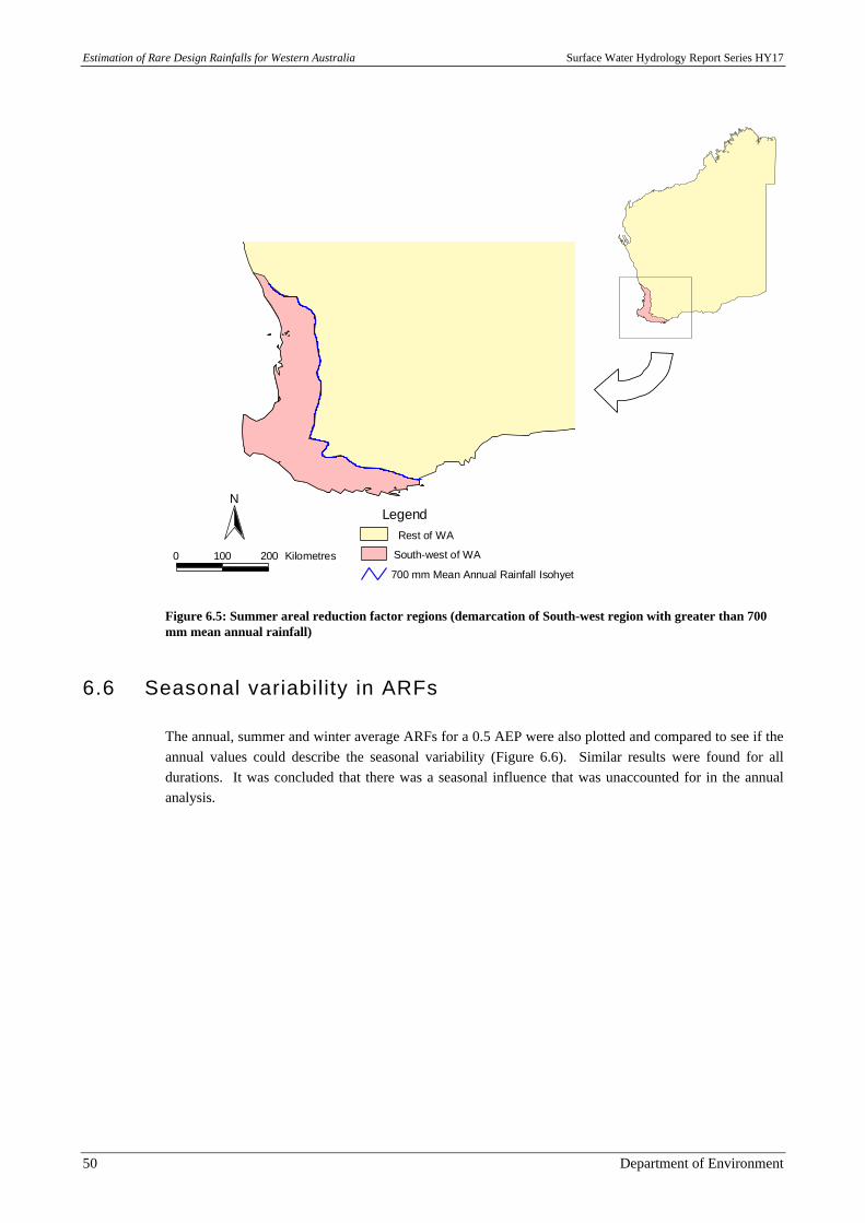
Estimation of Rare Design Rainfalls for Western Australia Surface Water Hydrology Report Series HY17
50 Department of Environment
LegendRest of WA
South-west of WA
700 mm Mean Annual Rainfall Isohyet
0 100 200 Kilometres
N
Figure 6.5: Summer areal reduction factor regions (demarcation of South-west region with greater than 700mm mean annual rainfall)
6.6 Seasonal variability in ARFs
The annual, summer and winter average ARFs for a 0.5 AEP were also plotted and compared to see if theannual values could describe the seasonal variability (Figure 6.6). Similar results were found for alldurations. It was concluded that there was a seasonal influence that was unaccounted for in the annualanalysis.
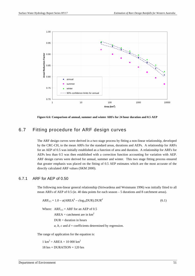
Surface Water Hydrology Report Series HY17 Estimation of Rare Design Rainfalls for Western Australia
Department of Environment 51
0.70
0.75
0.80
0.85
0.90
0.95
1.00
1 10 100 1000 10000
Area (km2)
Are
al R
edu
ctio
n F
acto
r
annual
summer
winter
90% confidence limits for annual
Figure 6.6: Comparison of annual, summer and winter ARFs for 24 hour duration and 0.5 AEP
6.7 Fitting procedure for ARF design curves
The ARF design curves were derived in a two stage process by fitting a non-linear relationship, developedby the CRC-CH, to the mean ARFs for the standard areas, durations and AEPs. A relationship for ARFsfor an AEP of 0.5 was initially established as a function of area and duration. A relationship for ARFs forAEPs less than 0.5 was then established with a correction function accounting for variation with AEP.ARF design curves were derived for annual, summer and winter. This two stage fitting process ensuredthat greater emphasis was placed on the fitting of 0.5 AEP estimates which are the most accurate of thedirectly calculated ARF values (SKM 2000).
6.7.1 ARF for AEP of 0.50
The following non-linear general relationship (Siriwardena and Weinmann 1996) was initially fitted to allmean ARFs of AEP of 0.5 (ie. 40 data points for each season – 5 durations and 8 catchment areas).
ARF0.5 = 1.0 – a(AREAb – clog10DUR).DURd (6.1)
Where: ARF0.5 = ARF for an AEP of 0.5
AREA = catchment are in km2
DUR = duration in hours
a, b, c and d = coefficients determined by regression.
The range of application for the equation is:
1 km2 = AREA = 10 000 km2
18 hrs = DURATION = 120 hrs
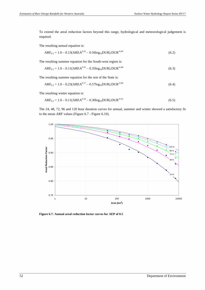
Estimation of Rare Design Rainfalls for Western Australia Surface Water Hydrology Report Series HY17
52 Department of Environment
To extend the areal reduction factors beyond this range, hydrological and meteorological judgement isrequired.
The resulting annual equation is:
ARF0.5 = 1.0 – 0.13(AREA0.21 – 0.56log10DUR).DUR-0.45 (6.2)
The resulting summer equation for the South-west region is:
ARF0.5 = 1.0 – 0.11(AREA0.25 – 0.35log10DUR).DUR-0.48 (6.3)
The resulting summer equation for the rest of the State is:
ARF0.5 = 1.0 – 0.23(AREA0.17 – 0.57log10DUR).DUR-0.40 (6.4)
The resulting winter equation is:
ARF0.5 = 1.0 – 0.11(AREA0.24 – 0.30log10DUR).DUR-0.52 (6.5)
The 24, 48, 72, 96 and 120 hour duration curves for annual, summer and winter showed a satisfactory fitto the mean ARF values (Figure 6.7 - Figure 6.10).
0.75
0.80
0.85
0.90
0.95
1.00
1 10 100 1000 10000
Area (km2)
Are
al R
edu
ctio
n F
acto
r
24 hr
48 hr
72 hr
96 hr
120 hr
Figure 6.7: Annual areal reduction factor curves for AEP of 0.5
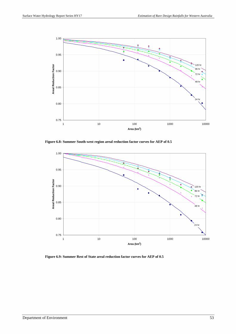
Surface Water Hydrology Report Series HY17 Estimation of Rare Design Rainfalls for Western Australia
Department of Environment 53
0.75
0.80
0.85
0.90
0.95
1.00
1 10 100 1000 10000
Area (km2)
Are
al R
edu
ctio
n F
acto
r
24 hr
48 hr
72 hr
96 hr
120 hr
Figure 6.8: Summer South-west region areal reduction factor curves for AEP of 0.5
0.75
0.80
0.85
0.90
0.95
1.00
1 10 100 1000 10000
Area (km2)
Are
al R
edu
ctio
n F
acto
r
24 hr
48 hr
72 hr
96 hr
120 hr
Figure 6.9: Summer Rest of State areal reduction factor curves for AEP of 0.5
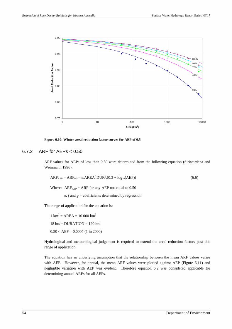
Estimation of Rare Design Rainfalls for Western Australia Surface Water Hydrology Report Series HY17
54 Department of Environment
0.75
0.80
0.85
0.90
0.95
1.00
1 10 100 1000 10000
Area (km2)
Are
al R
edu
ctio
n F
acto
r
24 hr
48 hr
72 hr
96 hr
120 hr
Figure 6.10: Winter areal reduction factor curves for AEP of 0.5
6.7.2 ARF for AEPs < 0.50
ARF values for AEPs of less than 0.50 were determined from the following equation (Siriwardena andWeinmann 1996).
ARFAEP = ARF0.5 – e.AREAf.DURg.(0.3 + log10(AEP)) (6.6)
Where: ARFAEP = ARF for any AEP not equal to 0.50
e, f and g = coefficients determined by regression
The range of application for the equation is:
1 km2 = AREA = 10 000 km2
18 hrs = DURATION = 120 hrs
0.50 < AEP = 0.0005 (1 in 2000)
Hydrological and meteorological judgement is required to extend the areal reduction factors past thisrange of application.
The equation has an underlying assumption that the relationship between the mean ARF values varieswith AEP. However, for annual, the mean ARF values were plotted against AEP (Figure 6.11) andnegligible variation with AEP was evident. Therefore equation 6.2 was considered applicable fordetermining annual ARFs for all AEPs.
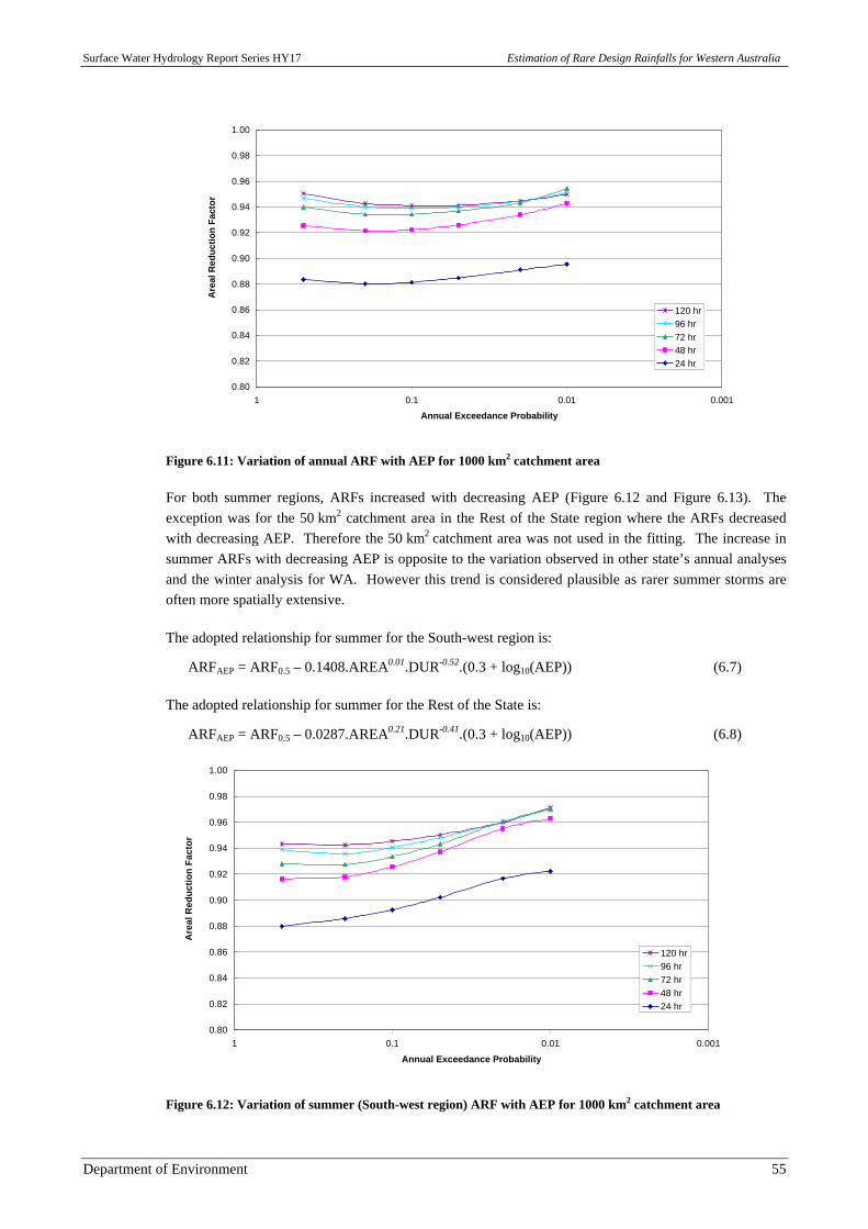
Surface Water Hydrology Report Series HY17 Estimation of Rare Design Rainfalls for Western Australia
Department of Environment 55
0.80
0.82
0.84
0.86
0.88
0.90
0.92
0.94
0.96
0.98
1.00
0.0010.010.11
Annual Exceedance Probability
Are
al R
edu
ctio
n F
acto
r
120 hr96 hr72 hr48 hr24 hr
Figure 6.11: Variation of annual ARF with AEP for 1000 km2 catchment area
For both summer regions, ARFs increased with decreasing AEP (Figure 6.12 and Figure 6.13). Theexception was for the 50 km2 catchment area in the Rest of the State region where the ARFs decreasedwith decreasing AEP. Therefore the 50 km2 catchment area was not used in the fitting. The increase insummer ARFs with decreasing AEP is opposite to the variation observed in other state’s annual analysesand the winter analysis for WA. However this trend is considered plausible as rarer summer storms areoften more spatially extensive.
The adopted relationship for summer for the South-west region is:
ARFAEP = ARF0.5 – 0.1408.AREA0.01.DUR-0.52.(0.3 + log10(AEP)) (6.7)
The adopted relationship for summer for the Rest of the State is:
ARFAEP = ARF0.5 – 0.0287.AREA0.21.DUR-0.41.(0.3 + log10(AEP)) (6.8)
0.80
0.82
0.84
0.86
0.88
0.90
0.92
0.94
0.96
0.98
1.00
0.0010.010.11
Annual Exceedance Probability
Are
al R
edu
ctio
n F
acto
r
120 hr96 hr72 hr48 hr24 hr
Figure 6.12: Variation of summer (South-west region) ARF with AEP for 1000 km2 catchment area
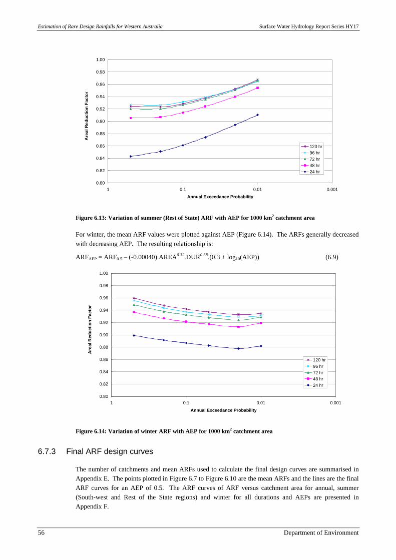
Estimation of Rare Design Rainfalls for Western Australia Surface Water Hydrology Report Series HY17
56 Department of Environment
0.80
0.82
0.84
0.86
0.88
0.90
0.92
0.94
0.96
0.98
1.00
0.0010.010.11
Annual Exceedance Probability
Are
al R
edu
ctio
n F
acto
r
120 hr96 hr72 hr48 hr24 hr
Figure 6.13: Variation of summer (Rest of State) ARF with AEP for 1000 km2 catchment area
For winter, the mean ARF values were plotted against AEP (Figure 6.14). The ARFs generally decreasedwith decreasing AEP. The resulting relationship is:
ARFAEP = ARF0.5 – (-0.00040).AREA0.32.DUR0.38.(0.3 + log10(AEP)) (6.9)
0.80
0.82
0.84
0.86
0.88
0.90
0.92
0.94
0.96
0.98
1.00
0.0010.010.11
Annual Exceedance Probability
Are
al R
edu
ctio
n F
acto
r
120 hr96 hr72 hr48 hr24 hr
Figure 6.14: Variation of winter ARF with AEP for 1000 km2 catchment area
6.7.3 Final ARF design curves
The number of catchments and mean ARFs used to calculate the final design curves are summarised inAppendix E. The points plotted in Figure 6.7 to Figure 6.10 are the mean ARFs and the lines are the finalARF curves for an AEP of 0.5. The ARF curves of ARF versus catchment area for annual, summer(South-west and Rest of the State regions) and winter for all durations and AEPs are presented inAppendix F.
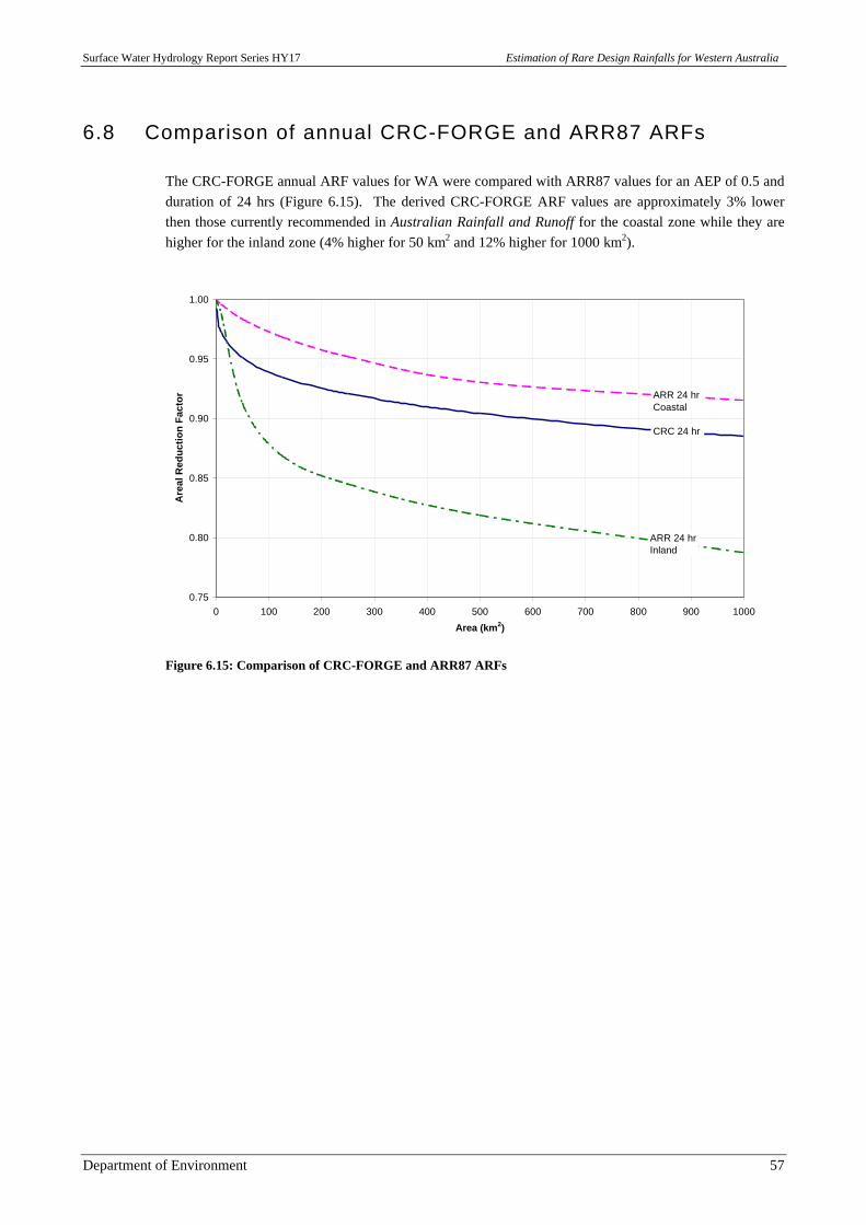
Surface Water Hydrology Report Series HY17 Estimation of Rare Design Rainfalls for Western Australia
Department of Environment 57
6.8 Comparison of annual CRC-FORGE and ARR87 ARFs
The CRC-FORGE annual ARF values for WA were compared with ARR87 values for an AEP of 0.5 andduration of 24 hrs (Figure 6.15). The derived CRC-FORGE ARF values are approximately 3% lowerthen those currently recommended in Australian Rainfall and Runoff for the coastal zone while they arehigher for the inland zone (4% higher for 50 km2 and 12% higher for 1000 km2).
0.75
0.80
0.85
0.90
0.95
1.00
0 100 200 300 400 500 600 700 800 900 1000
Area (km2)
Are
al R
edu
ctio
n F
acto
r
CRC 24 hr
ARR 24 hrCoastal
ARR 24 hrInland
Figure 6.15: Comparison of CRC-FORGE and ARR87 ARFs
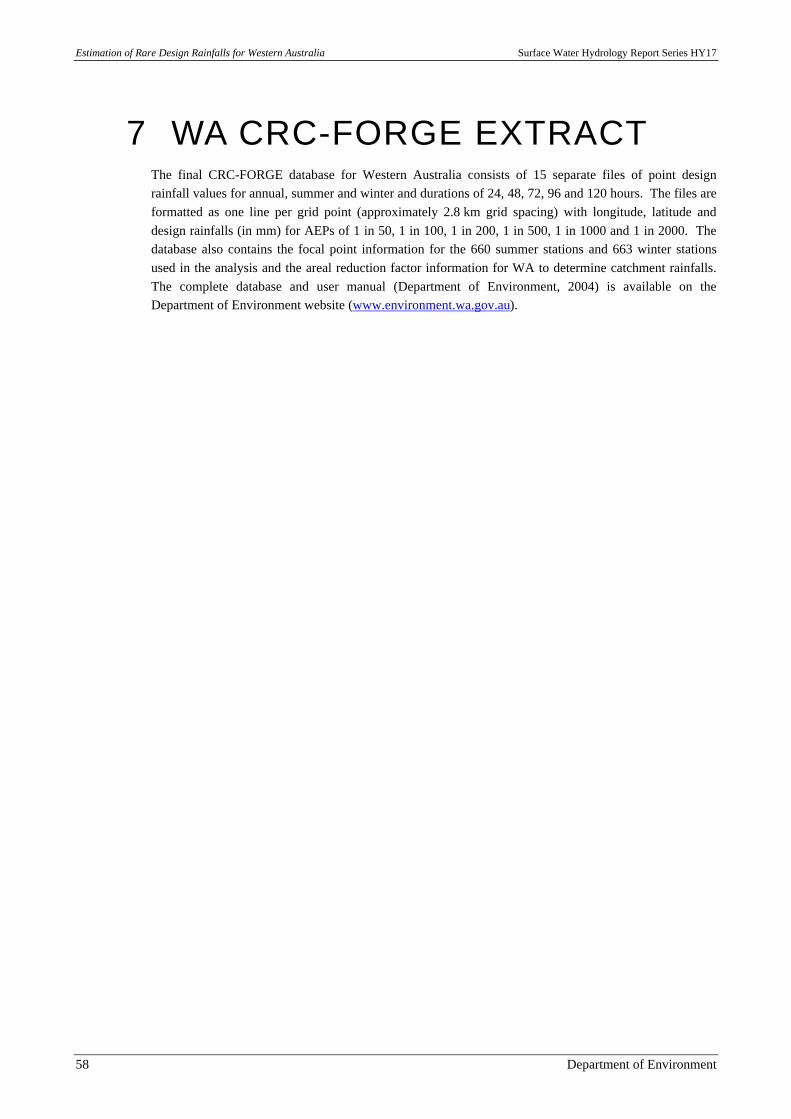
Estimation of Rare Design Rainfalls for Western Australia Surface Water Hydrology Report Series HY17
58 Department of Environment
7 WA CRC-FORGE EXTRACTThe final CRC-FORGE database for Western Australia consists of 15 separate files of point designrainfall values for annual, summer and winter and durations of 24, 48, 72, 96 and 120 hours. The files areformatted as one line per grid point (approximately 2.8 km grid spacing) with longitude, latitude anddesign rainfalls (in mm) for AEPs of 1 in 50, 1 in 100, 1 in 200, 1 in 500, 1 in 1000 and 1 in 2000. Thedatabase also contains the focal point information for the 660 summer stations and 663 winter stationsused in the analysis and the areal reduction factor information for WA to determine catchment rainfalls.The complete database and user manual (Department of Environment, 2004) is available on theDepartment of Environment website (www.environment.wa.gov.au).
Surface Water Hydrology Report Series HY17 Estimation of Rare Design Rainfalls for Western Australia
Department of Environment 59
8 Conclusions and recommendationsThe CRC-FORGE method of regional rainfall frequency analysis originally developed by the CooperativeResearch Centre for Catchment Hydrology (Nandakumar et al, 1997) has been successfully applied toWestern Australia, with significant modification.
For Western Australia, the CRC-FORGE methodology was applied annually and seasonally, for winterand summer to determine design point rainfalls. Revised areal reduction factors were also derived on anannual and seasonal basis to estimate catchment rainfalls. Significant modifications to the original CRC-FORGE methodology were required to adapt the CRC-FORGE approach for Western Australia’sseasonal analysis. The application of CRC-FORGE to Western Australia found that a number ofhomogenous regions were required and that a combination of the GEV and Pearson Type III (PE3)statistical distributions was needed to characterise the at-site rainfall across some of the regions in orderto calibrate the spatial dependence model.
It is intended that the database of WA CRC-FORGE rainfall estimates and areal reduction factors be usedin conjunction with the relevant information provided in Book II and Book VI of Australian Rainfall andRunoff. However, practitioners are urged to exercise caution when using this new information for WAtogether with existing recommendations in Australian Rainfall and Runoff.
The outcomes of the application of the CRC-FORGE approach to Western Australia are considered to bea significant improvement on current methods of rainfall estimation for WA, however the followingrecommendations may improve design rainfall estimates for WA further:
§ Investigate sparsely gauged areas further, including the use of data from short record stations and theeffects of non-concurrent records to improve estimates for these areas (Nandakumar et al, 1997);
§ Assess the differences between CRC-FORGE and ARR87 estimates at ungauged locations wherethere may be significant differences between the ANUSPLIN fitted surface and the ARR87 isolines;
§ Derive CRC-FORGE design rainfall estimates for durations shorter than 24 hours;
§ Derive areal reduction factors for durations shorter than 24 hours; and
§ Develop CRC-FORGE temporal patterns for design events in the large to rare range.

Surface Water Hydrology Report Series HY17 Estimation of Rare Design Rainfalls for Western Australia
Department of Environment 61
References and recommendedreading
Bureau of Meteorology. 1996, The Estimation of Probable Maximum Precipitation in Australia: Generalised Short-Duration Method, supplement to Bulletin 53, Australian Government Publishing Service, Canberra.
Bureau of Meteorology. 1997, Bureau of Meteorology Inspection Handbook (1967 - ), Annex 6, ObservationSpecification No. 2013, January 1997, pg. 69.
Canterford, R.P., Pescod, N.R., Pearce, H.J. and Turner, L.H. 1998, Book II Design Rainfall Considerations, AustralianRainfall and Runoff, Institution of Engineers, Australia.
Dales, M.Y. and Reed, D.W. 1989, ‘Regional flood and storm hazard assessment’, Report No 102, Institute ofHydrology, Wallingford, Oxon, UK.
Davies, F. and Chapman, N. 1997, Rainfall Transducers Users Guide, Water Information Bookshelf, Water and RiversCommission, Unpublished.
Department of Environment. 2004, User manual for the "WA CRC-FORGE EXTRACT" computer program,Department of Environment, Government of Western Australia, Surface Water Hydrology Series Report No. HY20.
Filliben, J.J. 1975, ‘The probability plot correlation coefficient test for normality’ Technometrics, 17(1).
Gamble, S. and McConachy, F. 1999, ‘Application of the Focussed Rainfall Growth Estimation Technique inTasmania’, Water 99 Joint Congress, Brisbane, Australia.
Hargraves, G. in prep, Extreme Rainfall Estimation Project, CRCFORGE and (CRC) ARF Techniques, Queensland andBorder Locations, Development and Application, Department of Natural Resources and Mines, Government ofQueensland.
Hosking, J.R.M. and Wallis, J.R. 1991, ‘Some Statistics Useful in Regional Frequency Analysis’, Mathematics, IBMResearch Division, New York.
Hutchinson, M.F. 2003, ANUSPLIN Version 4.2 User Guide, Centre for Resource and Environmental Studies, TheAustralian National university, Canberra.
Kuczera, G. 2000, FLIKE – Flood Frequency Analysis Program Version 4.5, Department of Civil, Surveying andEnvironmental Engineering, University of Newcastle, New South Wales.
Lu, L.H. and Stedinger, J.R. 1992, ‘Sampling variance of normalized GEV/PWM quantile estiamtors and a regionalhomogeneity test’ Journal of Hydrology, 138, pp. 223-245.
McGilchrist, C.A. and Woodeyer, K.D. 1975, ‘Note on a distribution free CUSUM technique’, Technometrics, 17(3),pp. 321-323/
Estimation of Rare Design Rainfalls for Western Australia Surface Water Hydrology Report Series HY17
62 Department of Environment
Nathan, R.J. and Weinmann, P.E. 1999, Book VI Estimation of Large to Extreme Floods, Australian Rainfall andRunoff, Institution of Engineers, Australia.
Nandakumar, N., Weinmann, P.E., Mein, R.G. and Nathan, R.J. 1997, Estimation of Extreme Rainfalls for VictoriaUsing the CRC-FORGE Method (For Rainfall Durations 24 to 72 Hours), Report 97/4.
Nandakumar, N., Weinmann, P.E., Mein, R.G. and Nathan, R.J. 2000, ‘Estimation of Spatial Dependence for the CRC-FORGE Method’, Hydro 2000 – 3rd International Hydrology and Water Resources Symposium, Perth, Australia.
Nandakumar, N., Schopf, J.M., Weinmann, P.E. and Ruprecht, J.K. 2004, ‘Estimation of Spatial Dependence forApplication of the CRC-FORGE Method in Western Australia’, extended abstract of paper presented at theInternational Conference on Storms, Brisbane, Australia.
Pearce, L.J. 1998, ‘Extreme Seasonal Rainfall Study’, Water and Rivers Commission, Surface Water Hydrology SeriesSWH14, Unpublished Report.
Ruprecht, J.K. and Karafilis, D.W. 1994, ‘Regional Flood Frequency – Caution Needed’, Paper submitted to WaterDown Under, Adelaide, Australia.
Siriwardena, L. and Weinmann, P.E. 1996, ‘Development and Testing of Methodology to Derive Areal ReductionFactors for Long Duration Rainfalls’, Cooperative Research Centre for Catchment Hydrology Working Document 96/4.
Siriwardena, L. and Weinmann, P.E. 1999, ‘Preparation of the CRC-FORGE Design Rainfall Database for Victoria’,Cooperative Research Centre for Catchment Hydrology Working Document 99/1.
SKM (Sinclair Knight Merz). 2000, Application of CRC-FORGE Method to South Australia Volume 1 - Estimation ofRare Design Rainfalls for SA Version 1.
Srikanthan, R. and Stewart, B.J. 1991, ‘Analysis of Australian rainfall data with respect to climate variability andchange’, Australian Meteorological Magazine, 39(1), pp. 11-20.
Weinmann, P.E., Nandakumar, N., Siriwardena, L., Mein, R.G. and Nathan, R.J. 1999, ‘Estimation of rare designrainfalls for Victoria using the CRC-FORGE methodology’, Water 99 Joint Congress, Brisbane, Australia.
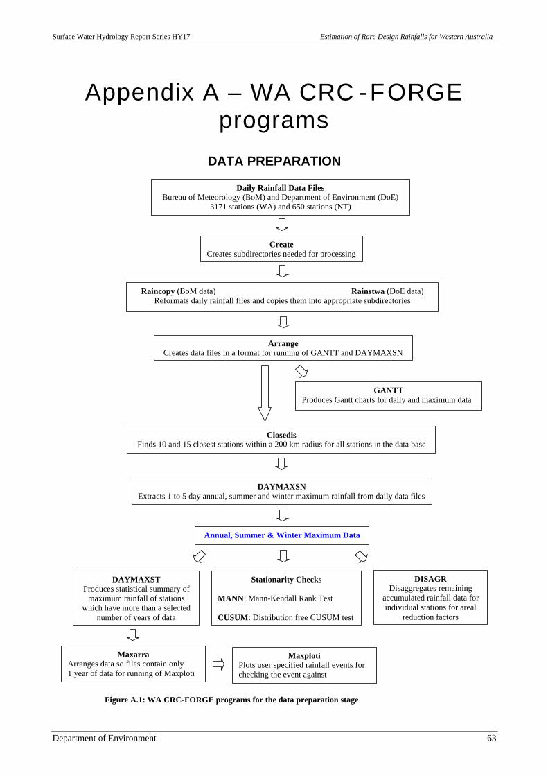
Surface Water Hydrology Report Series HY17 Estimation of Rare Design Rainfalls for Western Australia
Department of Environment 63
Appendix A – WA CRC -FORGEprograms
DATA PREPARATION
Daily Rainfall Data FilesBureau of Meteorology (BoM) and Department of Environment (DoE)
3171 stations (WA) and 650 stations (NT)
CreateCreates subdirectories needed for processing
Raincopy (BoM data) Rainstwa (DoE data)Reformats daily rainfall files and copies them into appropriate subdirectories
ArrangeCreates data files in a format for running of GANTT and DAYMAXSN
GANTTProduces Gantt charts for daily and maximum data
ClosedisFinds 10 and 15 closest stations within a 200 km radius for all stations in the data base
DAYMAXSNExtracts 1 to 5 day annual, summer and winter maximum rainfall from daily data files
Annual, Summer & Winter Maximum Data
DAYMAXSTProduces statistical summary of
maximum rainfall of stationswhich have more than a selected
number of years of data
Stationarity Checks
MANN: Mann-Kendall Rank Test
CUSUM: Distribution free CUSUM test
DISAGRDisaggregates remaining
accumulated rainfall data forindividual stations for areal
reduction factors
MaxarraArranges data so files contain only1 year of data for running of Maxploti
MaxplotiPlots user specified rainfall events forchecking the event againstneighbouring stations
Figure A.1: WA CRC-FORGE programs for the data preparation stage
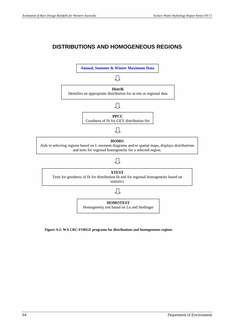
Estimation of Rare Design Rainfalls for Western Australia Surface Water Hydrology Report Series HY17
64 Department of Environment
DISTRIBUTIONS AND HOMOGENEOUS REGIONS
Annual, Summer & Winter Maximum Data
DistribIdentifies an appropriate distribution for at-site or regional data
PPCCGoodness of fit for GEV distribution fits
HOMOAids in selecting regions based on L-moment diagrams and/or spatial maps, displays distributions
and tests for regional homogeneity for a selected region.
XTESTTests for goodness of fit for distribution fit and for regional homogeneity based on
statisticsand software routines by Hosking and Wallis
HOMOTESTHomogeneity test based on Lu and Stedinger
Figure A.2: WA CRC-FORGE programs for distributions and homogeneous regions
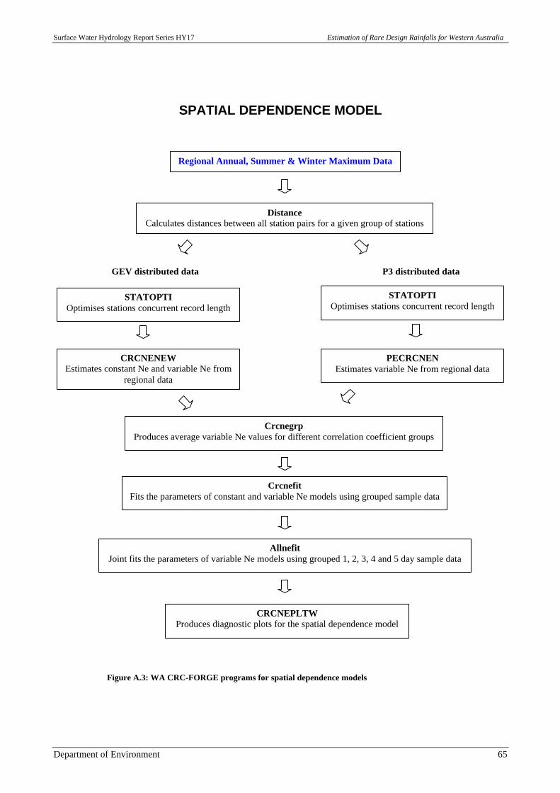
Surface Water Hydrology Report Series HY17 Estimation of Rare Design Rainfalls for Western Australia
Department of Environment 65
SPATIAL DEPENDENCE MODEL
Regional Annual, Summer & Winter Maximum Data
DistanceCalculates distances between all station pairs for a given group of stations
GEV distributed data P3 distributed data
STATOPTIOptimises stations concurrent record length
STATOPTIOptimises stations concurrent record length
CRCNENEWEstimates constant Ne and variable Ne from
regional data
PECRCNENEstimates variable Ne from regional data
CrcnegrpProduces average variable Ne values for different correlation coefficient groups
CrcnefitFits the parameters of constant and variable Ne models using grouped sample data
AllnefitJoint fits the parameters of variable Ne models using grouped 1, 2, 3, 4 and 5 day sample data
CRCNEPLTWProduces diagnostic plots for the spatial dependence model
Figure A.3: WA CRC-FORGE programs for spatial dependence models
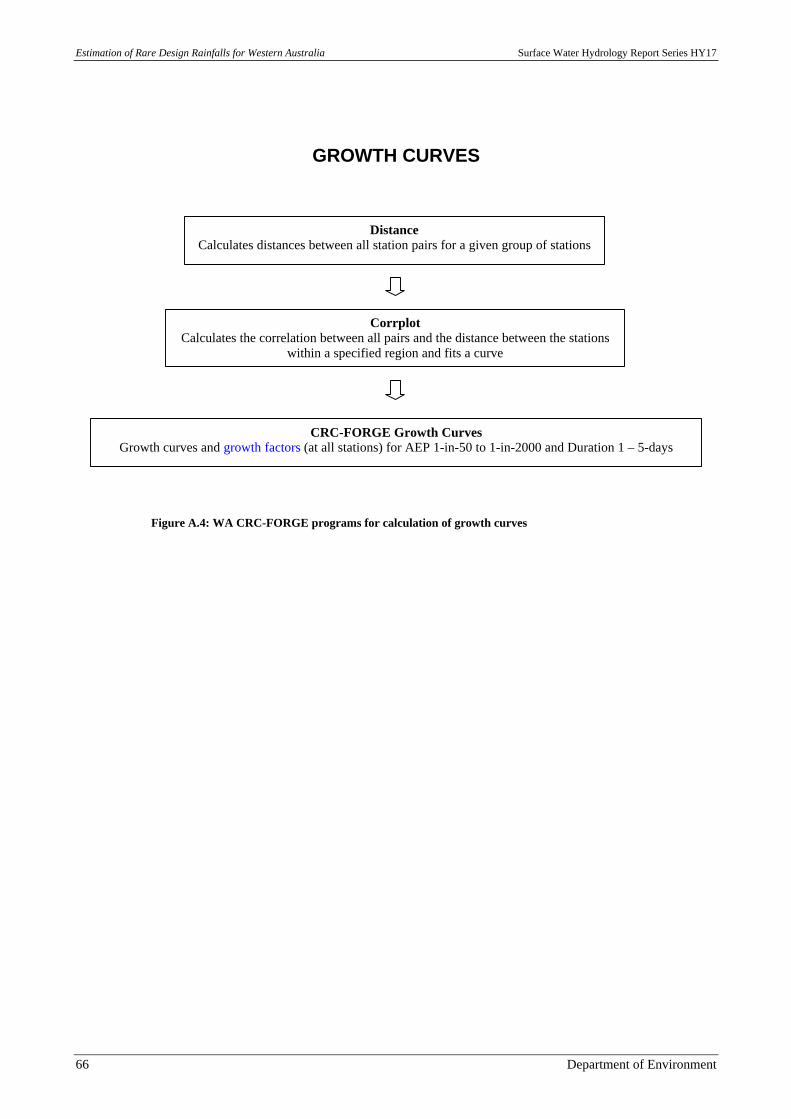
Estimation of Rare Design Rainfalls for Western Australia Surface Water Hydrology Report Series HY17
66 Department of Environment
GROWTH CURVES
DistanceCalculates distances between all station pairs for a given group of stations
CorrplotCalculates the correlation between all pairs and the distance between the stations
within a specified region and fits a curve
CRC-FORGE Growth CurvesGrowth curves and growth factors (at all stations) for AEP 1-in-50 to 1-in-2000 and Duration 1 – 5-days
Figure A.4: WA CRC-FORGE programs for calculation of growth curves
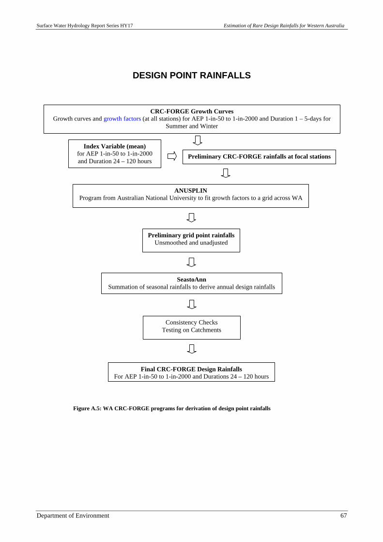
Surface Water Hydrology Report Series HY17 Estimation of Rare Design Rainfalls for Western Australia
Department of Environment 67
DESIGN POINT RAINFALLS
CRC-FORGE Growth CurvesGrowth curves and growth factors (at all stations) for AEP 1-in-50 to 1-in-2000 and Duration 1 – 5-days for
Summer and Winter
Index Variable (mean)for AEP 1-in-50 to 1-in-2000and Duration 24 – 120 hours
Preliminary CRC-FORGE rainfalls at focal stations
ANUSPLINProgram from Australian National University to fit growth factors to a grid across WA
Preliminary grid point rainfallsUnsmoothed and unadjusted
SeastoAnnSummation of seasonal rainfalls to derive annual design rainfalls
Consistency ChecksTesting on Catchments
Final CRC-FORGE Design RainfallsFor AEP 1-in-50 to 1-in-2000 and Durations 24 – 120 hours
Figure A.5: WA CRC-FORGE programs for derivation of design point rainfalls
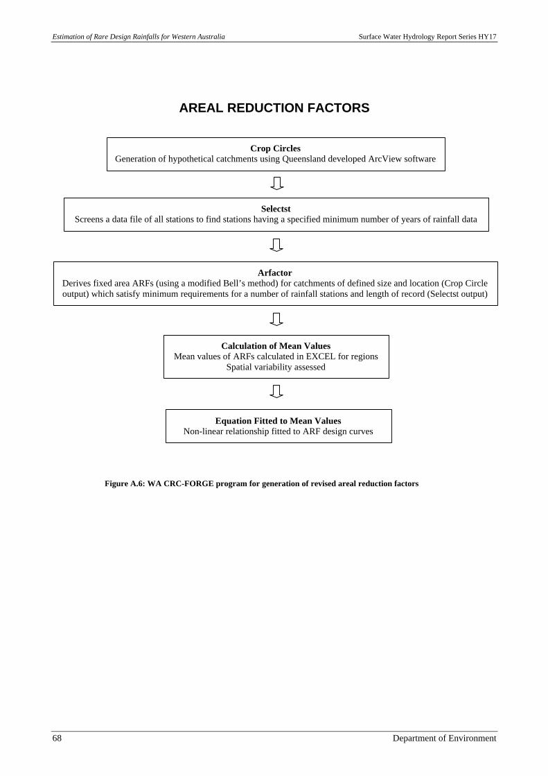
Estimation of Rare Design Rainfalls for Western Australia Surface Water Hydrology Report Series HY17
68 Department of Environment
AREAL REDUCTION FACTORS
Crop CirclesGeneration of hypothetical catchments using Queensland developed ArcView software
SelectstScreens a data file of all stations to find stations having a specified minimum number of years of rainfall data
ArfactorDerives fixed area ARFs (using a modified Bell’s method) for catchments of defined size and location (Crop Circleoutput) which satisfy minimum requirements for a number of rainfall stations and length of record (Selectst output)
Calculation of Mean ValuesMean values of ARFs calculated in EXCEL for regions
Spatial variability assessed
Equation Fitted to Mean ValuesNon-linear relationship fitted to ARF design curves
Figure A.6: WA CRC-FORGE program for generation of revised areal reduction factors
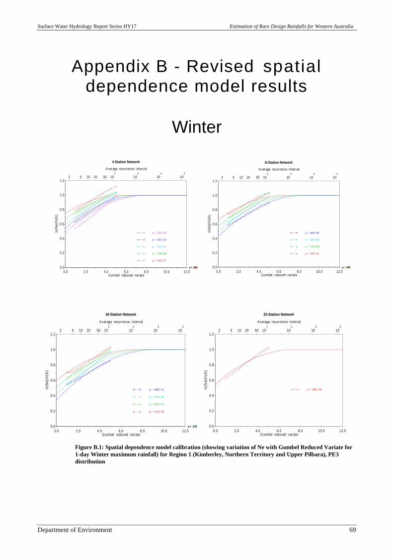
Surface Water Hydrology Report Series HY17 Estimation of Rare Design Rainfalls for Western Australia
Department of Environment 69
Appendix B - Revised spatialdependence model results
Winter
0.0 2.0 4.0 6.0 8.0 10.0 12.0Gumbel reduced var iate
2 5 10 20 50 102
103
104
105
A verage recurrence i nterval
0.0
0.2
0.4
0.6
0.8
1.0
1.2
ln(N
e)/ln
(N)
4-Station Network
ρ = .552 ( 34)
ρ= .552
ρ = .435 ( 56)
ρ= .435
ρ = .353 ( 91)
ρ= .353
ρ = .249 (106)
ρ= .249
ρ = .164 ( 57)
ρ= .164
0.0 2.0 4.0 6.0 8.0 10.0 12.0Gumbel reduced var iate
2 5 10 20 50 102
103
104
105
A verage recurrence i nterval
0.0
0.2
0.4
0.6
0.8
1.0
1.2
ln(N
e)/ln
(N)
8-Station Network
ρ = .444 ( 49)
ρ= .444
ρ = .345 (126)
ρ= .345
ρ = .256 (146)
ρ= .256
ρ = .169 ( 21)
ρ= .169
0.0 2.0 4.0 6.0 8.0 10.0 12.0Gum bel reduced var iate
2 5 10 20 50 102
103
104
105
A verage recurrence i nterval
0.0
0.2
0.4
0.6
0.8
1.0
1.2
ln(N
e)/ln
(N)
16-Station Network
ρ = .448 ( 31)
ρ= .448
ρ = .339 ( 44)
ρ= .339
ρ = .245 (111)
ρ= .245
ρ = .170 ( 59)
ρ= .170
0.0 2.0 4.0 6.0 8.0 10.0 12.0Gumbel reduced v ariate
2 5 10 20 50 102
103
104
105
A verage recurrence interv al
0.0
0.2
0.4
0.6
0.8
1.0
1.2
ln(N
e)/ln
(N)
32-Station Network
ρ = .166 ( 36)
Figure B.1: Spatial dependence model calibration (showing variation of Ne with Gumbel Reduced Variate for1-day Winter maximum rainfall) for Region 1 (Kimberley, Northern Territory and Upper Pilbara), PE3distribution
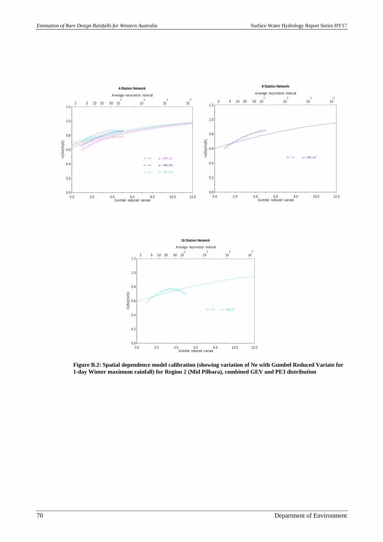
Estimation of Rare Design Rainfalls for Western Australia Surface Water Hydrology Report Series HY17
70 Department of Environment
0.0 2.0 4.0 6.0 8.0 10.0 12.0Gumbel reduced variate
2 5 10 20 50 102
103
104
105
A verage recurrence interval
0.0
0.2
0.4
0.6
0.8
1.0
1.2
ln(N
e)/ln
(N)
4-Station Network
ρ = .550 ( 21)
ρ = .446 ( 69)
ρ = .363 ( 44)
0.0 2.0 4.0 6.0 8.0 10.0 12.0Gumbel reduced variate
2 5 10 20 50 102
103
104
105
A verage recurrence interval
0.0
0.2
0.4
0.6
0.8
1.0
1.2
ln(N
e)/ln
(N)
8-Station Network
ρ = .455 ( 31)
0.0 2.0 4.0 6.0 8.0 10.0 12.0Gumbel reduced vari ate
2 5 10 20 50 102
103
104
105
A verage recurrence i nterval
0.0
0.2
0.4
0.6
0.8
1.0
1.2
ln(N
e)/ln
(N)
16-Station Network
ρ = .369 ( 32)
Figure B.2: Spatial dependence model calibration (showing variation of Ne with Gumbel Reduced Variate for1-day Winter maximum rainfall) for Region 2 (Mid Pilbara), combined GEV and PE3 distribution
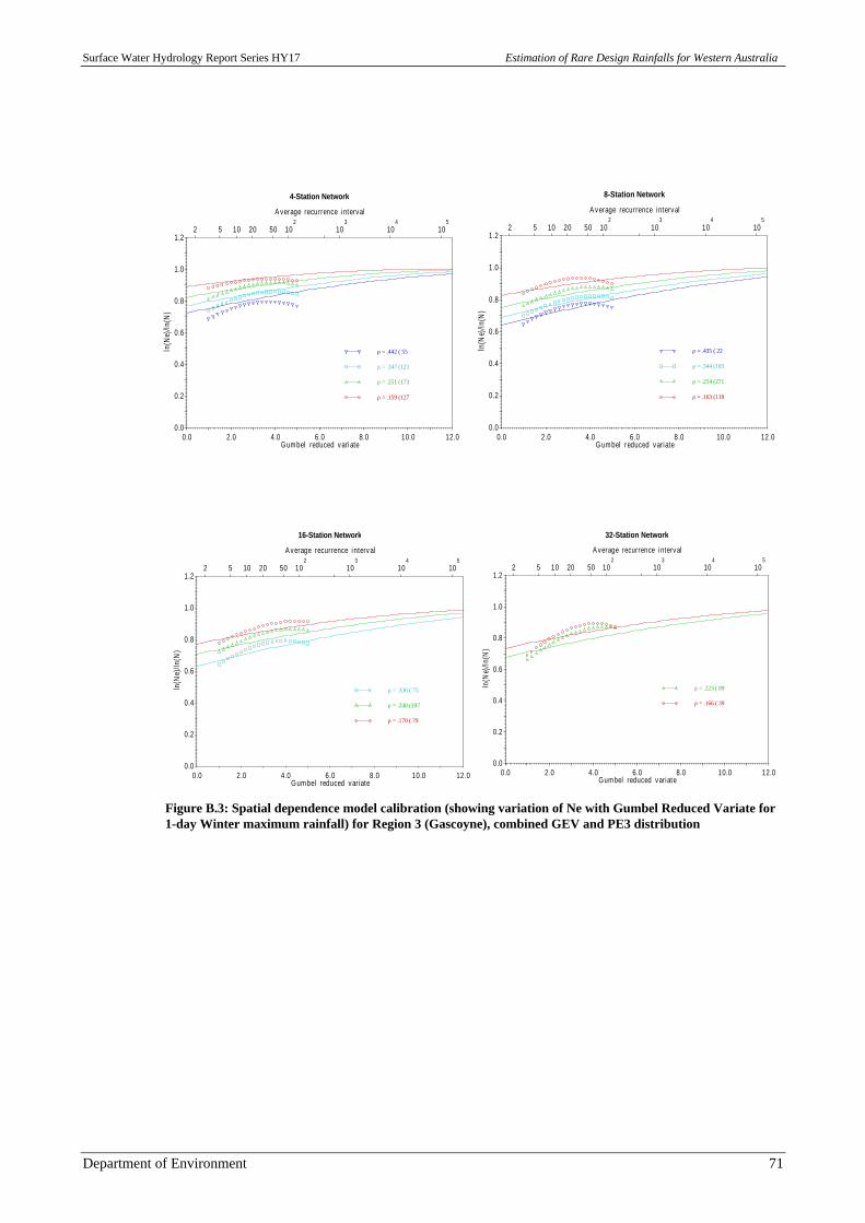
Surface Water Hydrology Report Series HY17 Estimation of Rare Design Rainfalls for Western Australia
Department of Environment 71
0.0 2.0 4.0 6.0 8.0 10.0 12.0Gumbel reduced vari ate
2 5 10 20 50 102
103
104
105
A verage recurrence i nterval
0.0
0.2
0.4
0.6
0.8
1.0
1.2
ln(N
e)/ln
(N)
4-Station Network
ρ = .442 ( 55)
ρ = .347 (123)
ρ = .251 (173)
ρ = .159 (127)
0.0 2.0 4.0 6.0 8.0 10.0 12.0Gumbel reduced variate
2 5 10 20 50 102
103
104
105
A verage recurrence i nterval
0.0
0.2
0.4
0.6
0.8
1.0
1.2
ln(N
e)/ln
(N)
8-Station Network
ρ = .435 ( 22)
ρ = .344 (103)
ρ = .254 (271)
ρ = .163 (118)
0.0 2.0 4.0 6.0 8.0 10.0 12.0Gumbel reduced variate
2 5 10 20 50 102
103
104
105
A verage recurrence i nterval
0.0
0.2
0.4
0.6
0.8
1.0
1.2
ln(N
e)/ln
(N)
16-Station Network
ρ = .336 ( 75)
ρ = .240 (197)
ρ = .170 ( 79)
0.0 2.0 4.0 6.0 8.0 10.0 12.0Gumbel reduced variate
2 5 10 20 50 102
103
104
105
A verage recurrence i nterval
0.0
0.2
0.4
0.6
0.8
1.0
1.2
ln(N
e)/ln
(N)
32-Station Network
ρ = .223 ( 89)
ρ = .166 ( 39)
Figure B.3: Spatial dependence model calibration (showing variation of Ne with Gumbel Reduced Variate for1-day Winter maximum rainfall) for Region 3 (Gascoyne), combined GEV and PE3 distribution
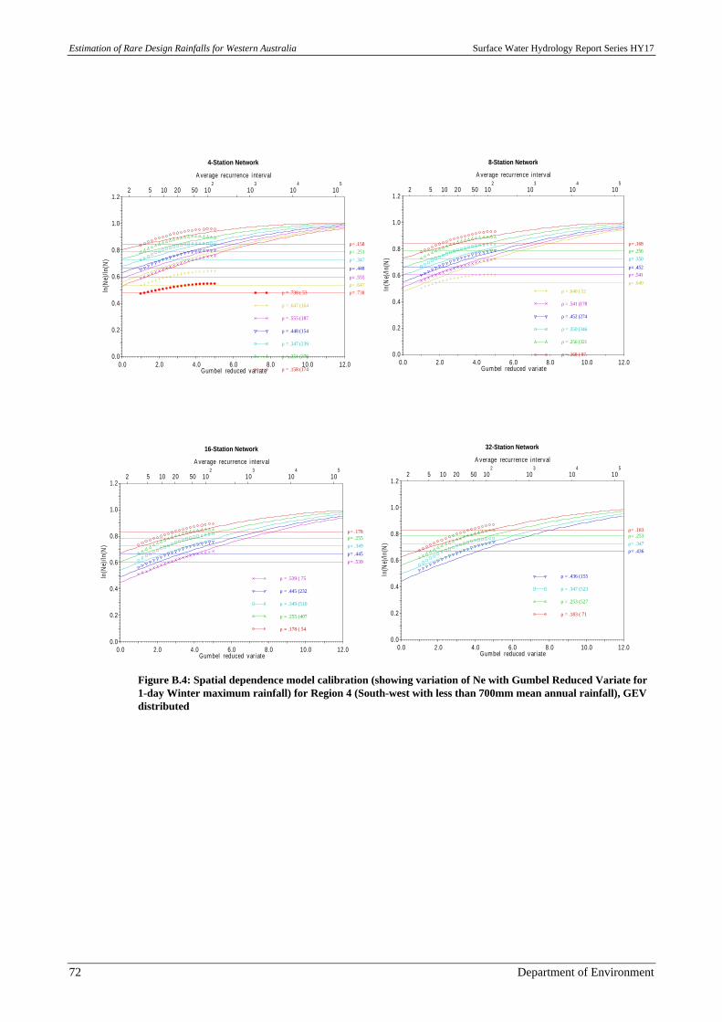
Estimation of Rare Design Rainfalls for Western Australia Surface Water Hydrology Report Series HY17
72 Department of Environment
0.0 2.0 4.0 6.0 8.0 10.0 12.0Gumbel reduced var iate
2 5 10 20 50 102
103
104
105
A verage recurrence i nterval
0.0
0.2
0.4
0.6
0.8
1.0
1.2
ln(N
e)/ln
(N)
4-Station Network
ρ = .738 ( 53) ρ= .738
ρ = .647 (164)
ρ= .647
ρ = .555 (187)
ρ= .555
ρ = .448 (154)
ρ= .448
ρ = .347 (239)
ρ= .347
ρ = .251 (270)
ρ= .251
ρ = .158 (174)
ρ= .158
0.0 2.0 4.0 6.0 8.0 10.0 12.0Gumbel reduced variate
2 5 10 20 50 102
103
104
105
A verage recurrence interval
0.0
0.2
0.4
0.6
0.8
1.0
1.2
ln(N
e)/ln
(N)
8-Station Network
ρ = .640 ( 52)
ρ= .640
ρ = .541 (178)
ρ= .541
ρ = .452 (274)
ρ= .452
ρ = .350 (346)
ρ= .350
ρ = .256 (321)
ρ= .256
ρ = .168 ( 97)
ρ= .168
0.0 2.0 4.0 6.0 8.0 10.0 12.0Gumbel reduced var iate
2 5 10 20 50 102
103
104
105
A verage recurrence i nterval
0.0
0.2
0.4
0.6
0.8
1.0
1.2
ln(N
e)/ln
(N)
16-Station Network
ρ = .539 ( 75)
ρ= .539
ρ = .445 (232)
ρ= .445
ρ = .349 (510)
ρ= .349
ρ = .255 (407)
ρ= .255
ρ = .178 ( 54)
ρ= .178
0.0 2.0 4.0 6.0 8.0 10.0 12.0Gumbel reduced var iate
2 5 10 20 50 102
103
104
105
A verage recurrence i nterval
0.0
0.2
0.4
0.6
0.8
1.0
1.2
ln(N
e)/ln
(N)
32-Station Network
ρ = .436 (155)
ρ= .436
ρ = .347 (523)
ρ= .347
ρ = .253 (527)
ρ= .253
ρ = .183 ( 71)
ρ= .183
Figure B.4: Spatial dependence model calibration (showing variation of Ne with Gumbel Reduced Variate for1-day Winter maximum rainfall) for Region 4 (South-west with less than 700mm mean annual rainfall), GEVdistributed
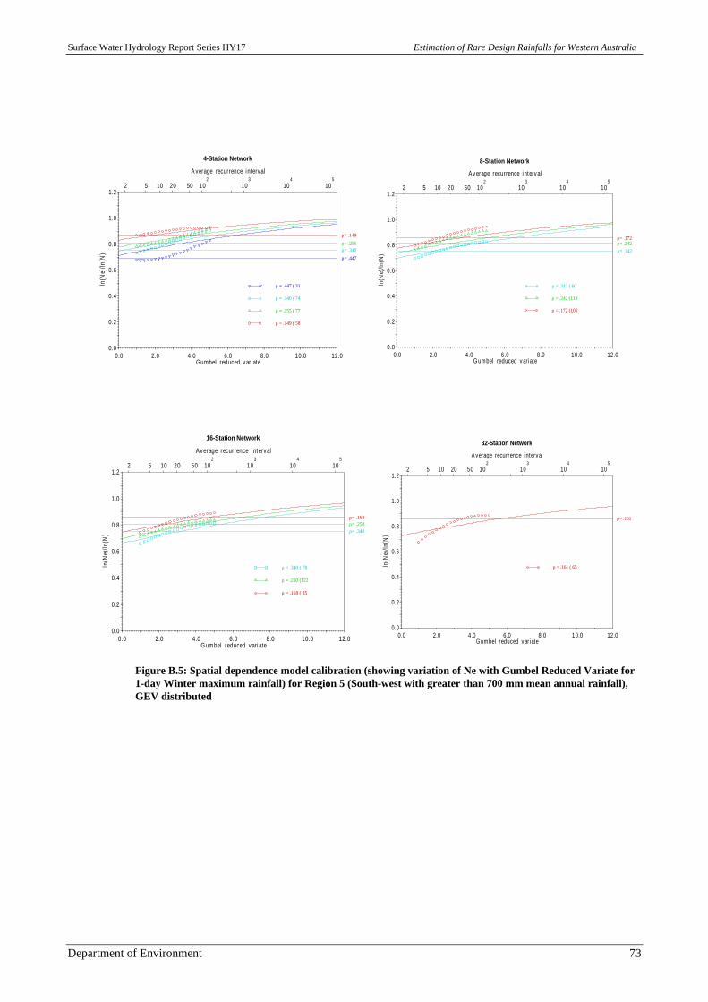
Surface Water Hydrology Report Series HY17 Estimation of Rare Design Rainfalls for Western Australia
Department of Environment 73
0.0 2.0 4.0 6.0 8.0 10.0 12.0Gumbel reduced var iate
2 5 10 20 50 102
103
104
105
A verage recurrence i nterval
0.0
0.2
0.4
0.6
0.8
1.0
1.2
ln(N
e)/ln
(N)
4-Station Network
ρ = .447 ( 31)
ρ= .447
ρ = .340 ( 74)
ρ= .340
ρ = .255 ( 77)
ρ= .255
ρ = .149 ( 58)
ρ= .149
0.0 2.0 4.0 6.0 8.0 10.0 12.0Gumbel reduced variate
2 5 10 20 50 102
103
104
105
A verage recurrence i nterval
0.0
0.2
0.4
0.6
0.8
1.0
1.2
ln(N
e)/ln
(N)
8-Station Network
ρ = .343 ( 60)
ρ= .343
ρ = .242 (119)
ρ= .242
ρ = .172 (105)
ρ= .172
0.0 2.0 4.0 6.0 8.0 10.0 12.0Gumbel reduced variate
2 5 10 20 50 102
103
104
105
Average recurrence interval
0.0
0.2
0.4
0.6
0.8
1.0
1.2
ln(N
e)/ln
(N)
16-Station Network
ρ = .340 ( 78)
ρ= .340
ρ = .250 (122)
ρ= .250
ρ = .168 ( 85)
ρ= .168
0.0 2.0 4.0 6.0 8.0 10.0 12.0Gumbel reduced v ariate
2 5 10 20 50 102
103
104
105
A verage recurrence i nterval
0.0
0.2
0.4
0.6
0.8
1.0
1.2
ln(N
e)/ln
(N)
32-Station Network
ρ = .161 ( 65)
ρ= .161
Figure B.5: Spatial dependence model calibration (showing variation of Ne with Gumbel Reduced Variate for1-day Winter maximum rainfall) for Region 5 (South-west with greater than 700 mm mean annual rainfall),GEV distributed
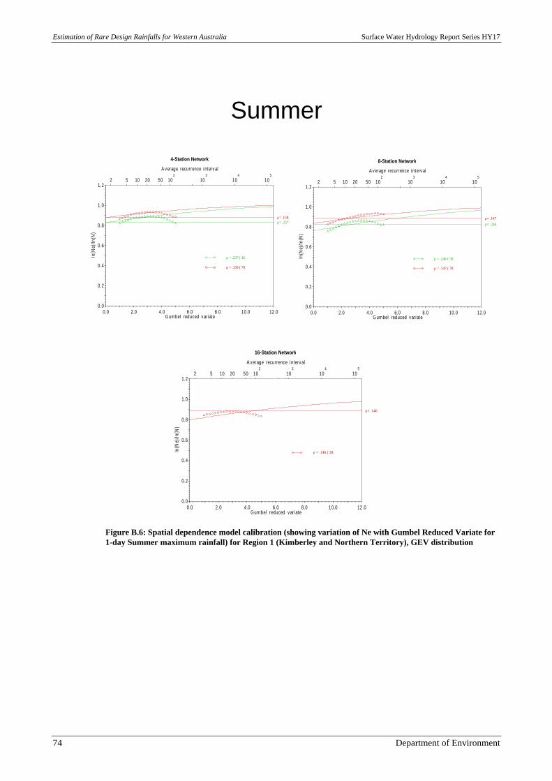
Estimation of Rare Design Rainfalls for Western Australia Surface Water Hydrology Report Series HY17
74 Department of Environment
Summer
0.0 2.0 4.0 6.0 8.0 10.0 12.0Gumbel reduced variate
2 5 10 20 50 102
103
104
105
A verage recurrence i nterval
0.0
0.2
0.4
0.6
0.8
1.0
1.2
ln(N
e)/ln
(N)
4-Station Network
ρ = .237 ( 42)
ρ= .237
ρ = .158 ( 78)
ρ= .158
0.0 2.0 4.0 6.0 8.0 10.0 12.0Gumbel reduced variate
2 5 10 20 50 102
103
104
105
A verage recurrence i nterval
0.0
0.2
0.4
0.6
0.8
1.0
1.2
ln(N
e)/ln
(N)
8-Station Network
ρ = .246 ( 58)
ρ= .246
ρ = .147 ( 78)
ρ= .147
0.0 2.0 4.0 6.0 8.0 10.0 12.0Gum bel reduced variate
2 5 10 20 50 102
103
104
105
A verage recurrence interval
0.0
0.2
0.4
0.6
0.8
1.0
1.2
ln(N
e)/ln
(N)
16-Station Network
ρ = .146 ( 28)
ρ= .146
Figure B.6: Spatial dependence model calibration (showing variation of Ne with Gumbel Reduced Variate for1-day Summer maximum rainfall) for Region 1 (Kimberley and Northern Territory), GEV distribution
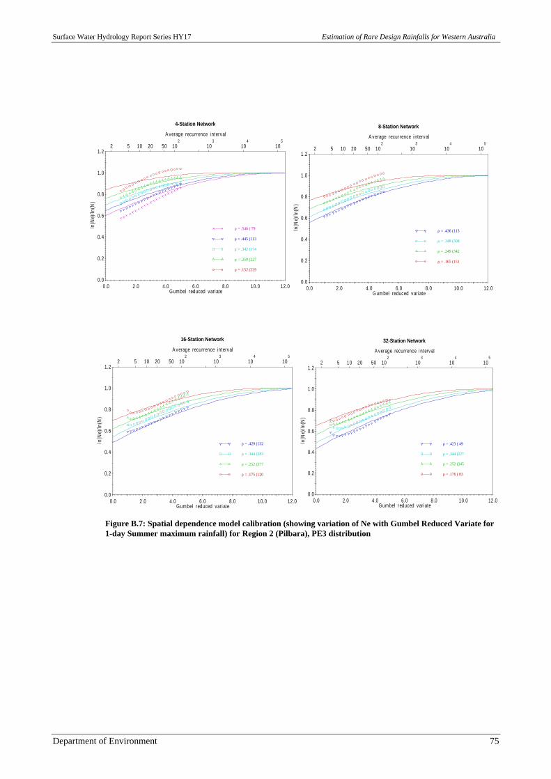
Surface Water Hydrology Report Series HY17 Estimation of Rare Design Rainfalls for Western Australia
Department of Environment 75
0.0 2.0 4.0 6.0 8.0 10.0 12.0Gumbel reduced variate
2 5 10 20 50 102
103
104
105
A verage recurrence interval
0.0
0.2
0.4
0.6
0.8
1.0
1.2
ln(N
e)/ln
(N)
4-Station Network
ρ = .546 ( 79)
ρ = .445 (113)
ρ = .342 (174)
ρ = .250 (227)
ρ = .152 (229)
0.0 2.0 4.0 6.0 8.0 10.0 12.0Gumbel reduced variate
2 5 10 20 50 102
103
104
105
A verage recurrence interval
0.0
0.2
0.4
0.6
0.8
1.0
1.2
ln(N
e)/ln
(N)
8-Station Network
ρ = .436 (113)
ρ = .348 (308)
ρ = .249 (342)
ρ = .165 (151)
0.0 2.0 4.0 6.0 8.0 10.0 12.0Gumbel reduced variate
2 5 10 20 50 102
103
104
105
A verage recurrence interval
0.0
0.2
0.4
0.6
0.8
1.0
1.2
ln(N
e)/ln
(N)
16-Station Network
ρ = .429 (132)
ρ = .344 (283)
ρ = .252 (377)
ρ = .175 (120)
0.0 2.0 4.0 6.0 8.0 10.0 12.0Gumbel reduced variate
2 5 10 20 50 102
103
104
105
A verage recurrence i nterval
0.0
0.2
0.4
0.6
0.8
1.0
1.2
ln(N
e)/ln
(N)
32-Station Network
ρ = .423 ( 49)
ρ = .344 (227)
ρ = .252 (345)
ρ = .176 ( 83)
Figure B.7: Spatial dependence model calibration (showing variation of Ne with Gumbel Reduced Variate for1-day Summer maximum rainfall) for Region 2 (Pilbara), PE3 distribution
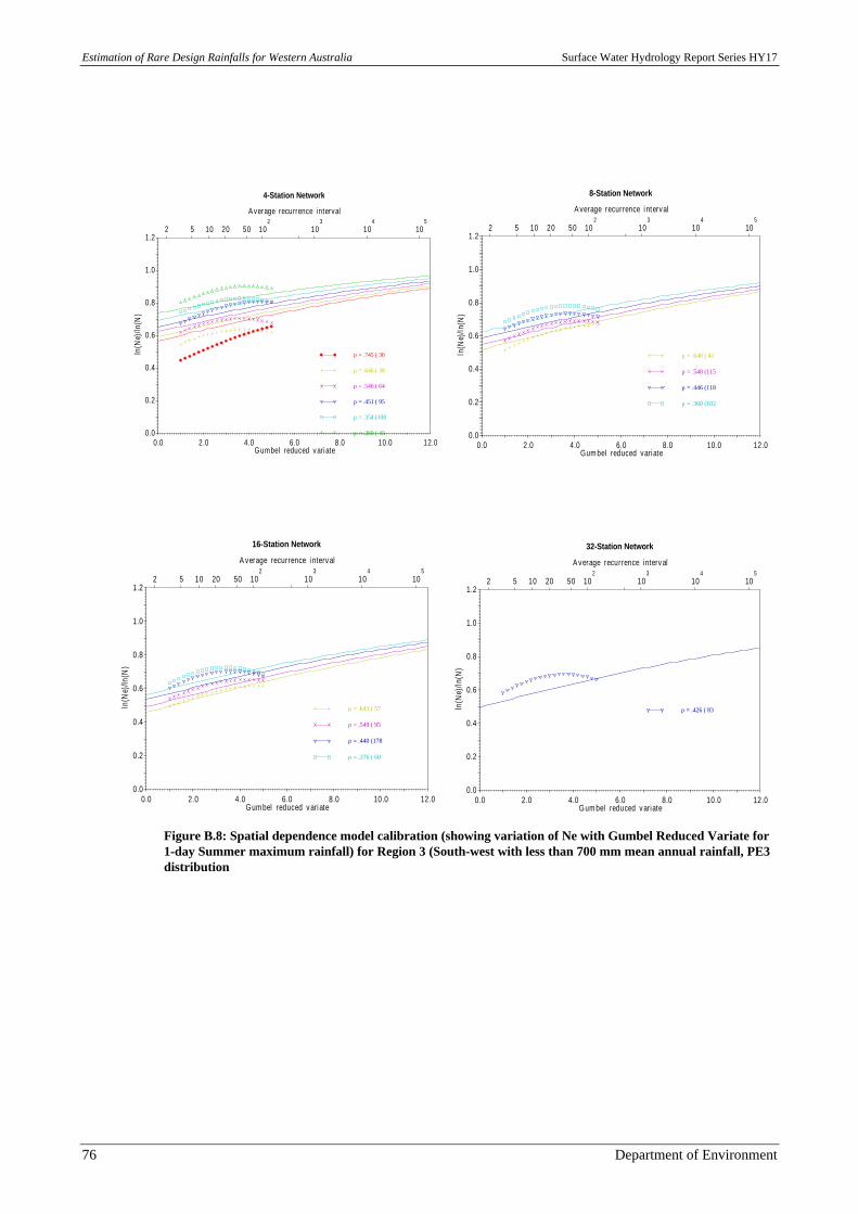
Estimation of Rare Design Rainfalls for Western Australia Surface Water Hydrology Report Series HY17
76 Department of Environment
0.0 2.0 4.0 6.0 8.0 10.0 12.0Gumbel reduced variate
2 5 10 20 50 102
103
104
105
A verage recurrence interval
0.0
0.2
0.4
0.6
0.8
1.0
1.2
ln(N
e)/ln
(N)
4-Station Network
ρ = .745 ( 36)
ρ = .646 ( 38)
ρ = .546 ( 64)
ρ = .451 ( 95)
ρ = .354 (108)
ρ = .269 ( 43)
0.0 2.0 4.0 6.0 8.0 10.0 12.0Gum bel reduced variate
2 5 10 20 50 102
103
104
105
A verage recurrence i nterval
0.0
0.2
0.4
0.6
0.8
1.0
1.2
ln(N
e)/ln
(N)
8-Station Network
ρ = .640 ( 41)
ρ = .548 (115)
ρ = .446 (118)
ρ = .360 (102)
0.0 2.0 4.0 6.0 8.0 10.0 12.0Gum bel reduced v ari ate
2 5 10 20 50 102
103
104
105
A verage recurrence i nterval
0.0
0.2
0.4
0.6
0.8
1.0
1.2
ln(N
e)/ln
(N)
16-Station Network
ρ = .643 ( 57)
ρ = .549 ( 95)
ρ = .440 (178)
ρ = .376 ( 60)
0.0 2.0 4.0 6.0 8.0 10.0 12.0Gum bel reduced v ariate
2 5 10 20 50 102
103
104
105
A verage recurrence i nterv al
0.0
0.2
0.4
0.6
0.8
1.0
1.2
ln(N
e)/ln
(N)
32-Station Network
ρ = .426 ( 83)
Figure B.8: Spatial dependence model calibration (showing variation of Ne with Gumbel Reduced Variate for1-day Summer maximum rainfall) for Region 3 (South-west with less than 700 mm mean annual rainfall, PE3distribution
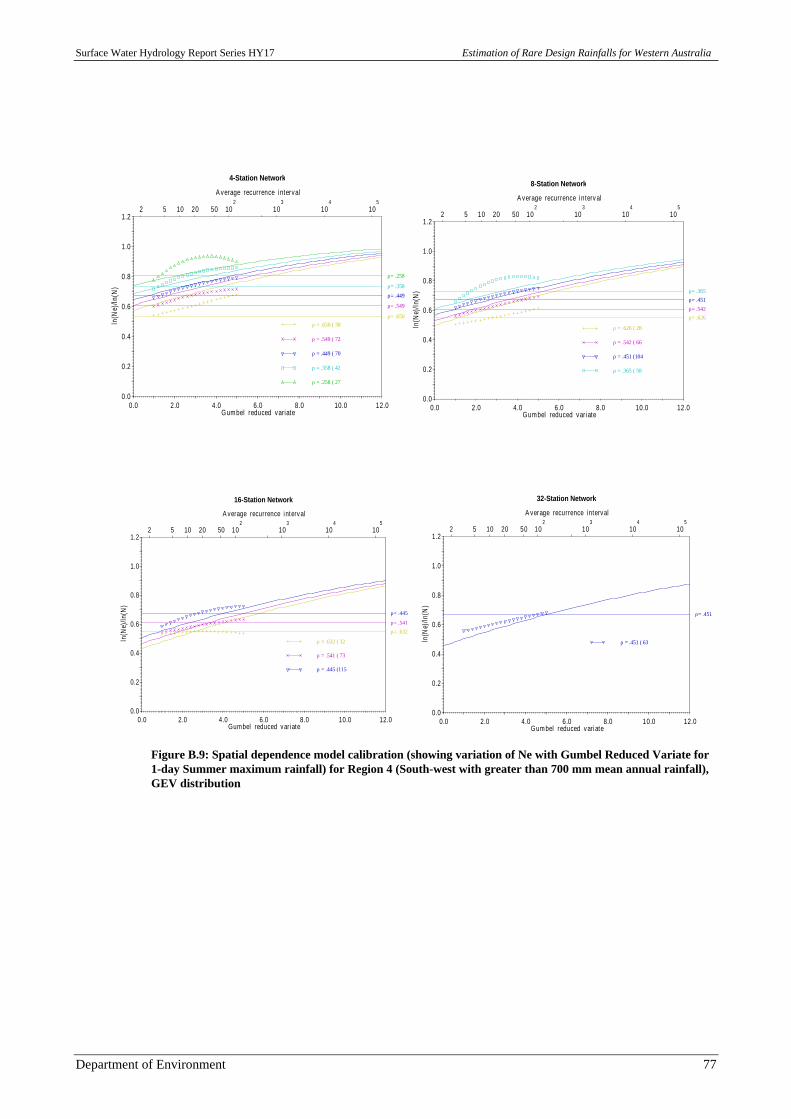
Surface Water Hydrology Report Series HY17 Estimation of Rare Design Rainfalls for Western Australia
Department of Environment 77
0.0 2.0 4.0 6.0 8.0 10.0 12.0Gumbel reduced variate
2 5 10 20 50 102
103
104
105
A verage recurrence interval
0.0
0.2
0.4
0.6
0.8
1.0
1.2
ln(N
e)/ln
(N)
4-Station Network
ρ = .650 ( 30)ρ= .650
ρ = .549 ( 72)
ρ= .549
ρ = .449 ( 70)
ρ= .449
ρ = .358 ( 42)
ρ= .358
ρ = .258 ( 27)
ρ= .258
0.0 2.0 4.0 6.0 8.0 10.0 12.0Gumbel reduced variate
2 5 10 20 50 102
103
104
105
A verage recurrence interv al
0.0
0.2
0.4
0.6
0.8
1.0
1.2
ln(N
e)/ln
(N)
8-Station Network
ρ = .626 ( 28)
ρ= .626
ρ = .542 ( 66)
ρ= .542
ρ = .451 (104)
ρ= .451
ρ = .365 ( 58)
ρ= .365
0.0 2.0 4.0 6.0 8.0 10.0 12.0Gumbel reduced var iate
2 5 10 20 50 102
103
104
105
A verage recurrence i nterval
0.0
0.2
0.4
0.6
0.8
1.0
1.2
ln(N
e)/ln
(N)
16-Station Network
ρ = .632 ( 32)
ρ= .632
ρ = .541 ( 73)
ρ= .541
ρ = .445 (115)
ρ= .445
0.0 2.0 4.0 6.0 8.0 10.0 12.0Gum bel reduced variate
2 5 10 20 50 102
103
104
105
A verage recurrence interval
0.0
0.2
0.4
0.6
0.8
1.0
1.2
ln(N
e)/ln
(N)
32-Station Network
ρ = .451 ( 63)
ρ= .451
Figure B.9: Spatial dependence model calibration (showing variation of Ne with Gumbel Reduced Variate for1-day Summer maximum rainfall) for Region 4 (South-west with greater than 700 mm mean annual rainfall),GEV distribution
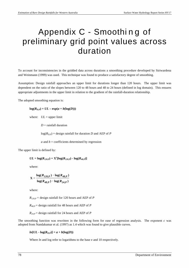
Estimation of Rare Design Rainfalls for Western Australia Surface Water Hydrology Report Series HY17
78 Department of Environment
Appendix C - Smoothi n g ofpreliminary grid point values across
duration
To account for inconsistencies in the gridded data across durations a smoothing procedure developed by Siriwardenaand Weinmann (1999) was used. This technique was found to produce a satisfactory degree of smoothing.
Assumption: Design rainfall approaches an upper limit for durations longer than 120 hours. The upper limit wasdependent on the ratio of the slopes between 120 to 48 hours and 48 to 24 hours (defined in log domain). This ensuresappropriate adjustments in the upper limit in relation to the gradient of the rainfall-duration relationship.
The adopted smoothing equation is:
log(RD,P) = UL – exp(a + b(log(D)))
where: UL = upper limit
D = rainfall duration
log(RD,P) = design rainfall for duration D and AEP of P
a and b = coefficients determined by regression
The upper limit is defined by:
UL = log(R120,P) + Xc[log(R120,P) - log(R48,P)]
where:
)log()log(
)log()log(X
P24,P48,
P48,P120,
RR
RR
−
−=
where:
R120,P = design rainfall for 120 hours and AEP of P
R48,P = design rainfall for 48 hours and AEP of P
R24,P = design rainfall for 24 hours and AEP of P
The smoothing function was rewritten in the following form for ease of regression analysis. The exponent c wasadopted from Nandakumar et al. (1997) as 1.4 which was found to give plausible curves.
ln[UL - log(RD,P)] = a + b(log(D))
Where ln and log refer to logarithms to the base e and 10 respectively.
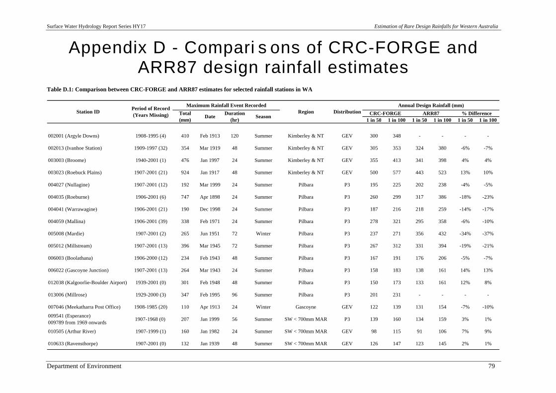
Surface Water Hydrology Report Series HY17 Estimation of Rare Design Rainfalls for Western Australia
Department of Environment 79
Appendix D - Compari s ons of CRC-FORGE andARR87 design rainfall estimates
Table D.1: Comparison between CRC-FORGE and ARR87 estimates for selected rainfall stations in WA
1 in 50 1 in 100 1 in 50 1 in 100 1 in 50 1 in 100
002001 (Argyle Downs) 1908-1995 (4) 410 Feb 1913 120 Summer Kimberley & NT GEV 300 348 - - - -
002013 (Ivanhoe Station) 1909-1997 (32) 354 Mar 1919 48 Summer Kimberley & NT GEV 305 353 324 380 -6% -7%
003003 (Broome) 1940-2001 (1) 476 Jan 1997 24 Summer Kimberley & NT GEV 355 413 341 398 4% 4%
003023 (Roebuck Plains) 1907-2001 (21) 924 Jan 1917 48 Summer Kimberley & NT GEV 500 577 443 523 13% 10%
004027 (Nullagine) 1907-2001 (12) 192 Mar 1999 24 Summer Pilbara P3 195 225 202 238 -4% -5%
004035 (Roeburne) 1906-2001 (6) 747 Apr 1898 24 Summer Pilbara P3 260 299 317 386 -18% -23%
004041 (Warrawagine) 1906-2001 (21) 190 Dec 1998 24 Summer Pilbara P3 187 216 218 259 -14% -17%
004059 (Mallina) 1906-2001 (39) 338 Feb 1971 24 Summer Pilbara P3 278 321 295 358 -6% -10%
005008 (Mardie) 1907-2001 (2) 265 Jun 1951 72 Winter Pilbara P3 237 271 356 432 -34% -37%
005012 (Millstream) 1907-2001 (13) 396 Mar 1945 72 Summer Pilbara P3 267 312 331 394 -19% -21%
006003 (Boolathana) 1906-2000 (12) 234 Feb 1943 48 Summer Pilbara P3 167 191 176 206 -5% -7%
006022 (Gascoyne Junction) 1907-2001 (13) 264 Mar 1943 24 Summer Pilbara P3 158 183 138 161 14% 13%
012038 (Kalgoorlie-Boulder Airport) 1939-2001 (0) 301 Feb 1948 48 Summer Pilbara P3 150 173 133 161 12% 8%
013006 (Millrose) 1929-2000 (3) 347 Feb 1995 96 Summer Pilbara P3 201 231 - - - -
007046 (Meekatharra Post Office) 1908-1985 (20) 110 Apr 1913 24 Winter Gascoyne GEV 122 139 131 154 -7% -10%
009541 (Esperance)009789 from 1969 onwards
1907-1968 (0) 207 Jan 1999 56 Summer SW < 700mm MAR P3 139 160 134 159 3% 1%
010505 (Arthur River) 1907-1999 (1) 160 Jan 1982 24 Summer SW < 700mm MAR GEV 98 115 91 106 7% 9%
010633 (Ravensthorpe) 1907-2001 (0) 132 Jan 1939 48 Summer SW < 700mm MAR GEV 126 147 123 145 2% 1%
DistributionAnnual Design Rainfall (mm)
Total (mm)
DateDuration
(hr)Season CRC-FORGE ARR87 % Difference
Period of Record (Years Missing)
Maximum Rainfall Event RecordedRegionStation ID
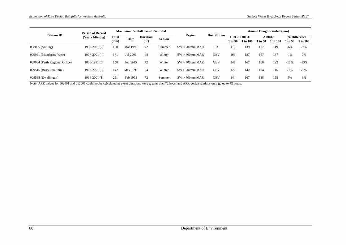
Estimation of Rare Design Rainfalls for Western Australia Surface Water Hydrology Report Series HY17
80 Department of Environment
1 in 50 1 in 100 1 in 50 1 in 100 1 in 50 1 in 100
008085 (Milling) 1930-2001 (2) 188 Mar 1999 72 Summer SW < 700mm MAR P3 119 139 127 149 -6% -7%
009031 (Mundaring Weir) 1907-2001 (4) 171 Jul 2001 48 Winter SW > 700mm MAR GEV 166 187 167 187 -1% 0%
009034 (Perth Regional Office) 1880-1991 (0) 158 Jun 1945 72 Winter SW > 700mm MAR GEV 149 167 168 192 -11% -13%
009515 (Busselton Shire) 1907-2001 (3) 142 May 1991 24 Winter SW > 700mm MAR GEV 126 142 104 116 21% 23%
009538 (Dwellingup) 1934-2001 (1) 251 Feb 1955 72 Summer SW > 700mm MAR GEV 144 167 138 155 5% 8%
Note: ARR values for 002001 and 013006 could not be calculated as event durations were greater than 72 hours and ARR design rainfalls only go up to 72 hours.
Station IDPeriod of Record (Years Missing)
Maximum Rainfall Event RecordedRegion Distribution
Annual Design Rainfall (mm)
Total (mm)
DateDuration
(hr)Season
CRC-FORGE ARR87 % Difference
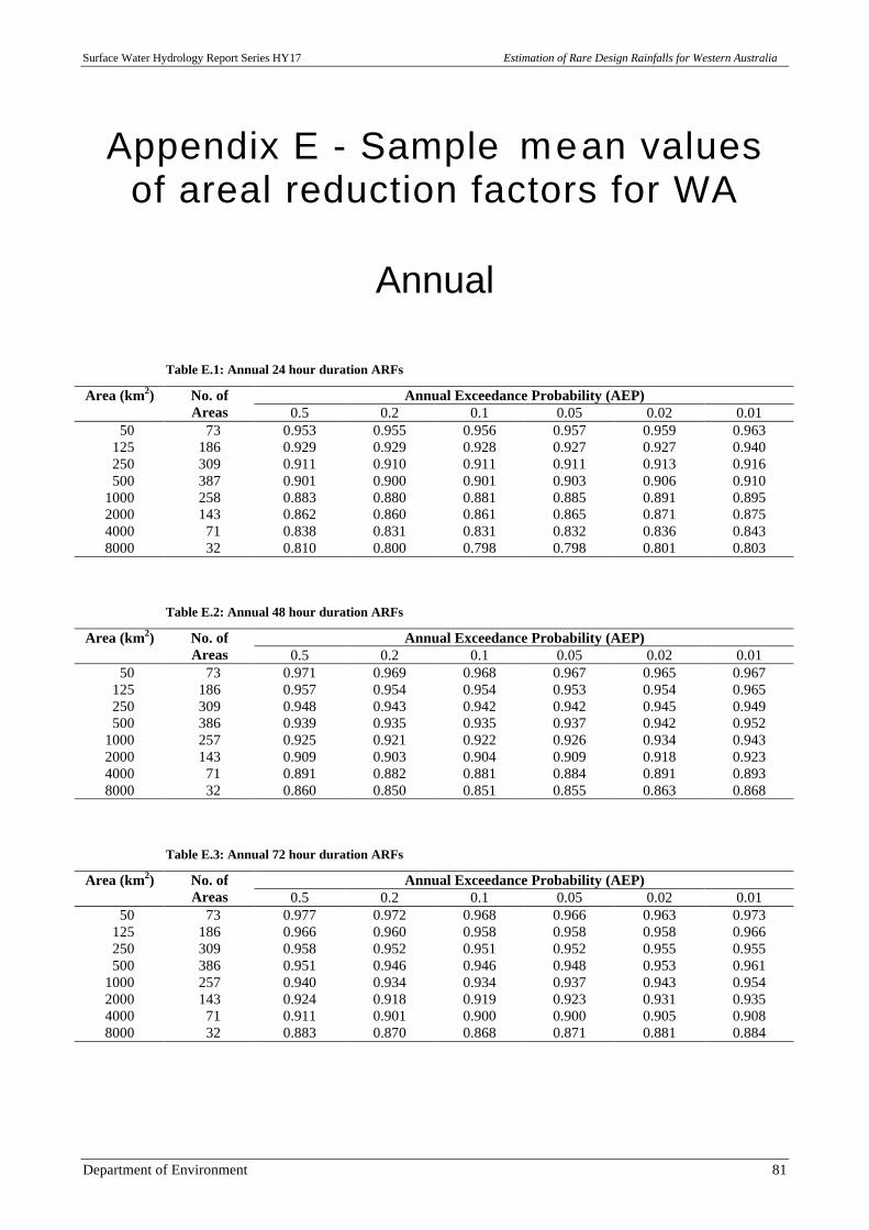
Surface Water Hydrology Report Series HY17 Estimation of Rare Design Rainfalls for Western Australia
Department of Environment 81
Appendix E - Sample mean valuesof areal reduction factors for WA
Annual
Table E.1: Annual 24 hour duration ARFs
Annual Exceedance Probability (AEP)Area (km2) No. ofAreas 0.5 0.2 0.1 0.05 0.02 0.01
50 73 0.953 0.955 0.956 0.957 0.959 0.963 125 186 0.929 0.929 0.928 0.927 0.927 0.940 250 309 0.911 0.910 0.911 0.911 0.913 0.916 500 387 0.901 0.900 0.901 0.903 0.906 0.9101000 258 0.883 0.880 0.881 0.885 0.891 0.8952000 143 0.862 0.860 0.861 0.865 0.871 0.8754000 71 0.838 0.831 0.831 0.832 0.836 0.8438000 32 0.810 0.800 0.798 0.798 0.801 0.803
Table E.2: Annual 48 hour duration ARFs
Annual Exceedance Probability (AEP)Area (km2) No. ofAreas 0.5 0.2 0.1 0.05 0.02 0.01
50 73 0.971 0.969 0.968 0.967 0.965 0.967 125 186 0.957 0.954 0.954 0.953 0.954 0.965 250 309 0.948 0.943 0.942 0.942 0.945 0.949 500 386 0.939 0.935 0.935 0.937 0.942 0.9521000 257 0.925 0.921 0.922 0.926 0.934 0.9432000 143 0.909 0.903 0.904 0.909 0.918 0.9234000 71 0.891 0.882 0.881 0.884 0.891 0.8938000 32 0.860 0.850 0.851 0.855 0.863 0.868
Table E.3: Annual 72 hour duration ARFs
Annual Exceedance Probability (AEP)Area (km2) No. ofAreas 0.5 0.2 0.1 0.05 0.02 0.01
50 73 0.977 0.972 0.968 0.966 0.963 0.973 125 186 0.966 0.960 0.958 0.958 0.958 0.966 250 309 0.958 0.952 0.951 0.952 0.955 0.955 500 386 0.951 0.946 0.946 0.948 0.953 0.9611000 257 0.940 0.934 0.934 0.937 0.943 0.9542000 143 0.924 0.918 0.919 0.923 0.931 0.9354000 71 0.911 0.901 0.900 0.900 0.905 0.9088000 32 0.883 0.870 0.868 0.871 0.881 0.884
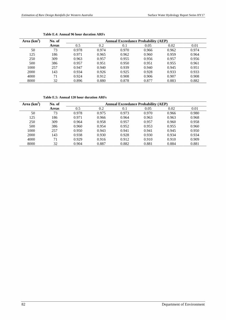
Estimation of Rare Design Rainfalls for Western Australia Surface Water Hydrology Report Series HY17
82 Department of Environment
Table E.4: Annual 96 hour duration ARFs
Annual Exceedance Probability (AEP)Area (km2) No. ofAreas 0.5 0.2 0.1 0.05 0.02 0.01
50 73 0.978 0.974 0.970 0.966 0.962 0.974 125 186 0.971 0.965 0.962 0.960 0.959 0.964 250 309 0.963 0.957 0.955 0.956 0.957 0.956 500 386 0.957 0.951 0.950 0.951 0.955 0.9611000 257 0.947 0.940 0.939 0.940 0.945 0.9512000 143 0.934 0.926 0.925 0.928 0.933 0.9334000 71 0.924 0.912 0.908 0.906 0.907 0.9088000 32 0.896 0.880 0.878 0.877 0.883 0.882
Table E.5: Annual 120 hour duration ARFs
Annual Exceedance Probability (AEP)Area (km2) No. ofAreas 0.5 0.2 0.1 0.05 0.02 0.01
50 73 0.978 0.975 0.973 0.970 0.966 0.980 125 186 0.971 0.966 0.964 0.963 0.963 0.968 250 309 0.964 0.958 0.957 0.957 0.960 0.958 500 386 0.960 0.954 0.952 0.953 0.955 0.9601000 257 0.950 0.943 0.941 0.941 0.945 0.9502000 143 0.938 0.930 0.928 0.930 0.934 0.9344000 71 0.929 0.916 0.912 0.910 0.910 0.9098000 32 0.904 0.887 0.882 0.881 0.884 0.881
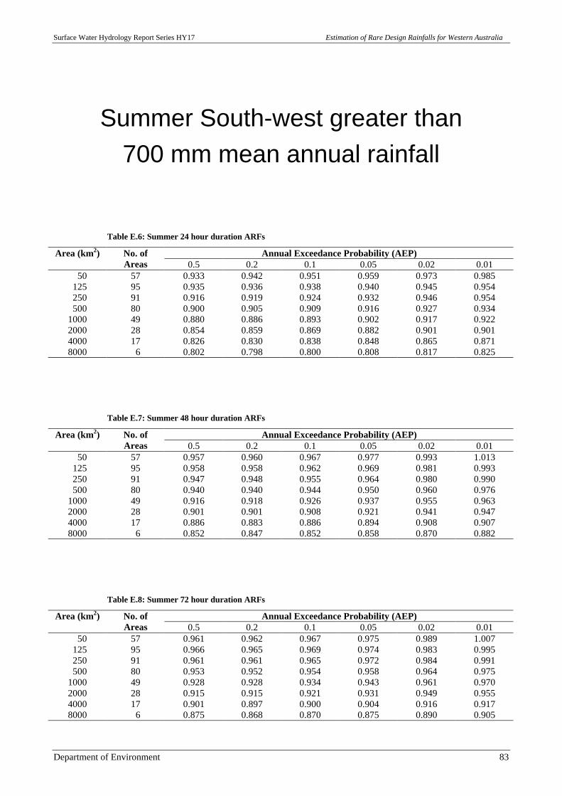
Surface Water Hydrology Report Series HY17 Estimation of Rare Design Rainfalls for Western Australia
Department of Environment 83
Summer South-west greater than700 mm mean annual rainfall
Table E.6: Summer 24 hour duration ARFs
Annual Exceedance Probability (AEP)Area (km2) No. ofAreas 0.5 0.2 0.1 0.05 0.02 0.01
50 57 0.933 0.942 0.951 0.959 0.973 0.985 125 95 0.935 0.936 0.938 0.940 0.945 0.954 250 91 0.916 0.919 0.924 0.932 0.946 0.954 500 80 0.900 0.905 0.909 0.916 0.927 0.9341000 49 0.880 0.886 0.893 0.902 0.917 0.9222000 28 0.854 0.859 0.869 0.882 0.901 0.9014000 17 0.826 0.830 0.838 0.848 0.865 0.8718000 6 0.802 0.798 0.800 0.808 0.817 0.825
Table E.7: Summer 48 hour duration ARFs
Annual Exceedance Probability (AEP)Area (km2) No. ofAreas 0.5 0.2 0.1 0.05 0.02 0.01
50 57 0.957 0.960 0.967 0.977 0.993 1.013 125 95 0.958 0.958 0.962 0.969 0.981 0.993 250 91 0.947 0.948 0.955 0.964 0.980 0.990 500 80 0.940 0.940 0.944 0.950 0.960 0.9761000 49 0.916 0.918 0.926 0.937 0.955 0.9632000 28 0.901 0.901 0.908 0.921 0.941 0.9474000 17 0.886 0.883 0.886 0.894 0.908 0.9078000 6 0.852 0.847 0.852 0.858 0.870 0.882
Table E.8: Summer 72 hour duration ARFs
Annual Exceedance Probability (AEP)Area (km2) No. ofAreas 0.5 0.2 0.1 0.05 0.02 0.01
50 57 0.961 0.962 0.967 0.975 0.989 1.007 125 95 0.966 0.965 0.969 0.974 0.983 0.995 250 91 0.961 0.961 0.965 0.972 0.984 0.991 500 80 0.953 0.952 0.954 0.958 0.964 0.9751000 49 0.928 0.928 0.934 0.943 0.961 0.9702000 28 0.915 0.915 0.921 0.931 0.949 0.9554000 17 0.901 0.897 0.900 0.904 0.916 0.9178000 6 0.875 0.868 0.870 0.875 0.890 0.905
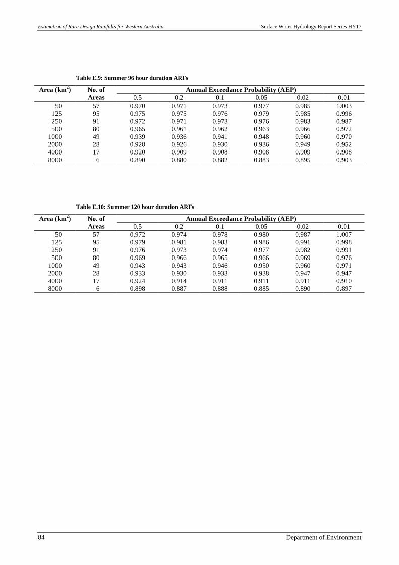
Estimation of Rare Design Rainfalls for Western Australia Surface Water Hydrology Report Series HY17
84 Department of Environment
Table E.9: Summer 96 hour duration ARFs
Annual Exceedance Probability (AEP)Area (km2) No. ofAreas 0.5 0.2 0.1 0.05 0.02 0.01
50 57 0.970 0.971 0.973 0.977 0.985 1.003 125 95 0.975 0.975 0.976 0.979 0.985 0.996 250 91 0.972 0.971 0.973 0.976 0.983 0.987 500 80 0.965 0.961 0.962 0.963 0.966 0.9721000 49 0.939 0.936 0.941 0.948 0.960 0.9702000 28 0.928 0.926 0.930 0.936 0.949 0.9524000 17 0.920 0.909 0.908 0.908 0.909 0.9088000 6 0.890 0.880 0.882 0.883 0.895 0.903
Table E.10: Summer 120 hour duration ARFs
Annual Exceedance Probability (AEP)Area (km2) No. ofAreas 0.5 0.2 0.1 0.05 0.02 0.01
50 57 0.972 0.974 0.978 0.980 0.987 1.007 125 95 0.979 0.981 0.983 0.986 0.991 0.998 250 91 0.976 0.973 0.974 0.977 0.982 0.991 500 80 0.969 0.966 0.965 0.966 0.969 0.9761000 49 0.943 0.943 0.946 0.950 0.960 0.9712000 28 0.933 0.930 0.933 0.938 0.947 0.9474000 17 0.924 0.914 0.911 0.911 0.911 0.9108000 6 0.898 0.887 0.888 0.885 0.890 0.897
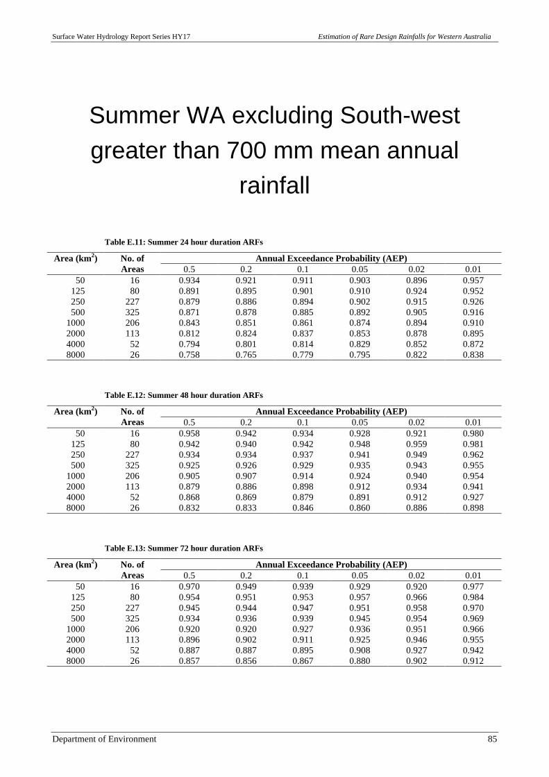
Surface Water Hydrology Report Series HY17 Estimation of Rare Design Rainfalls for Western Australia
Department of Environment 85
Summer WA excluding South-westgreater than 700 mm mean annual
rainfall
Table E.11: Summer 24 hour duration ARFs
Annual Exceedance Probability (AEP)Area (km2) No. ofAreas 0.5 0.2 0.1 0.05 0.02 0.01
50 16 0.934 0.921 0.911 0.903 0.896 0.957 125 80 0.891 0.895 0.901 0.910 0.924 0.952 250 227 0.879 0.886 0.894 0.902 0.915 0.926 500 325 0.871 0.878 0.885 0.892 0.905 0.9161000 206 0.843 0.851 0.861 0.874 0.894 0.9102000 113 0.812 0.824 0.837 0.853 0.878 0.8954000 52 0.794 0.801 0.814 0.829 0.852 0.8728000 26 0.758 0.765 0.779 0.795 0.822 0.838
Table E.12: Summer 48 hour duration ARFs
Annual Exceedance Probability (AEP)Area (km2) No. ofAreas 0.5 0.2 0.1 0.05 0.02 0.01
50 16 0.958 0.942 0.934 0.928 0.921 0.980 125 80 0.942 0.940 0.942 0.948 0.959 0.981 250 227 0.934 0.934 0.937 0.941 0.949 0.962 500 325 0.925 0.926 0.929 0.935 0.943 0.9551000 206 0.905 0.907 0.914 0.924 0.940 0.9542000 113 0.879 0.886 0.898 0.912 0.934 0.9414000 52 0.868 0.869 0.879 0.891 0.912 0.9278000 26 0.832 0.833 0.846 0.860 0.886 0.898
Table E.13: Summer 72 hour duration ARFs
Annual Exceedance Probability (AEP)Area (km2) No. ofAreas 0.5 0.2 0.1 0.05 0.02 0.01
50 16 0.970 0.949 0.939 0.929 0.920 0.977 125 80 0.954 0.951 0.953 0.957 0.966 0.984 250 227 0.945 0.944 0.947 0.951 0.958 0.970 500 325 0.934 0.936 0.939 0.945 0.954 0.9691000 206 0.920 0.920 0.927 0.936 0.951 0.9662000 113 0.896 0.902 0.911 0.925 0.946 0.9554000 52 0.887 0.887 0.895 0.908 0.927 0.9428000 26 0.857 0.856 0.867 0.880 0.902 0.912
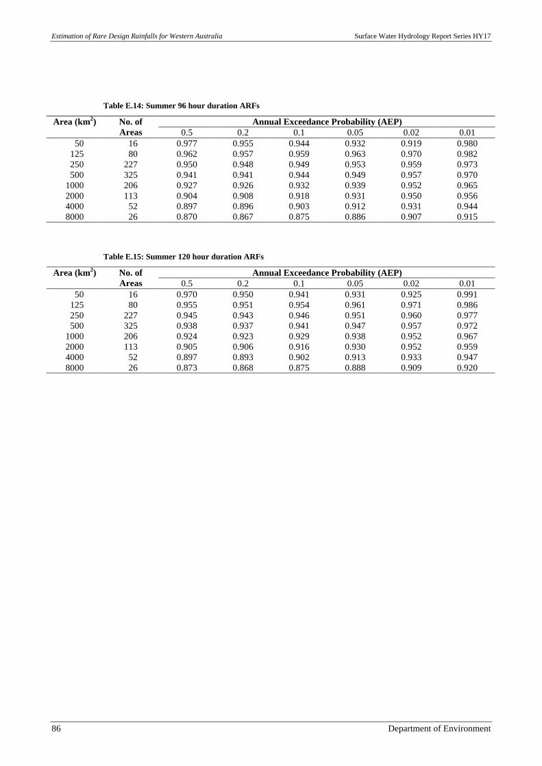
Estimation of Rare Design Rainfalls for Western Australia Surface Water Hydrology Report Series HY17
86 Department of Environment
Table E.14: Summer 96 hour duration ARFs
Annual Exceedance Probability (AEP)Area (km2) No. ofAreas 0.5 0.2 0.1 0.05 0.02 0.01
50 16 0.977 0.955 0.944 0.932 0.919 0.980 125 80 0.962 0.957 0.959 0.963 0.970 0.982 250 227 0.950 0.948 0.949 0.953 0.959 0.973 500 325 0.941 0.941 0.944 0.949 0.957 0.9701000 206 0.927 0.926 0.932 0.939 0.952 0.9652000 113 0.904 0.908 0.918 0.931 0.950 0.9564000 52 0.897 0.896 0.903 0.912 0.931 0.9448000 26 0.870 0.867 0.875 0.886 0.907 0.915
Table E.15: Summer 120 hour duration ARFs
Annual Exceedance Probability (AEP)Area (km2) No. ofAreas 0.5 0.2 0.1 0.05 0.02 0.01
50 16 0.970 0.950 0.941 0.931 0.925 0.991 125 80 0.955 0.951 0.954 0.961 0.971 0.986 250 227 0.945 0.943 0.946 0.951 0.960 0.977 500 325 0.938 0.937 0.941 0.947 0.957 0.9721000 206 0.924 0.923 0.929 0.938 0.952 0.9672000 113 0.905 0.906 0.916 0.930 0.952 0.9594000 52 0.897 0.893 0.902 0.913 0.933 0.9478000 26 0.873 0.868 0.875 0.888 0.909 0.920
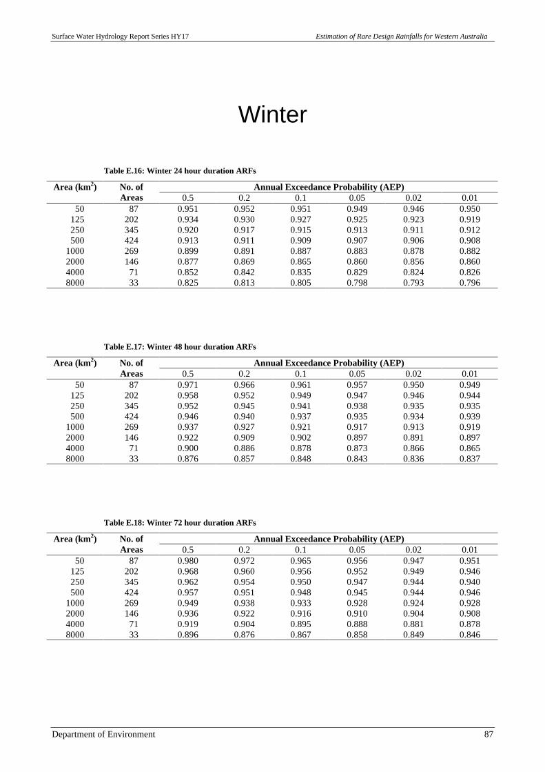
Surface Water Hydrology Report Series HY17 Estimation of Rare Design Rainfalls for Western Australia
Department of Environment 87
Winter
Table E.16: Winter 24 hour duration ARFs
Annual Exceedance Probability (AEP)Area (km2) No. ofAreas 0.5 0.2 0.1 0.05 0.02 0.01
50 87 0.951 0.952 0.951 0.949 0.946 0.950 125 202 0.934 0.930 0.927 0.925 0.923 0.919 250 345 0.920 0.917 0.915 0.913 0.911 0.912 500 424 0.913 0.911 0.909 0.907 0.906 0.9081000 269 0.899 0.891 0.887 0.883 0.878 0.8822000 146 0.877 0.869 0.865 0.860 0.856 0.8604000 71 0.852 0.842 0.835 0.829 0.824 0.8268000 33 0.825 0.813 0.805 0.798 0.793 0.796
Table E.17: Winter 48 hour duration ARFs
Annual Exceedance Probability (AEP)Area (km2) No. ofAreas 0.5 0.2 0.1 0.05 0.02 0.01
50 87 0.971 0.966 0.961 0.957 0.950 0.949 125 202 0.958 0.952 0.949 0.947 0.946 0.944 250 345 0.952 0.945 0.941 0.938 0.935 0.935 500 424 0.946 0.940 0.937 0.935 0.934 0.9391000 269 0.937 0.927 0.921 0.917 0.913 0.9192000 146 0.922 0.909 0.902 0.897 0.891 0.8974000 71 0.900 0.886 0.878 0.873 0.866 0.8658000 33 0.876 0.857 0.848 0.843 0.836 0.837
Table E.18: Winter 72 hour duration ARFs
Annual Exceedance Probability (AEP)Area (km2) No. ofAreas 0.5 0.2 0.1 0.05 0.02 0.01
50 87 0.980 0.972 0.965 0.956 0.947 0.951 125 202 0.968 0.960 0.956 0.952 0.949 0.946 250 345 0.962 0.954 0.950 0.947 0.944 0.940 500 424 0.957 0.951 0.948 0.945 0.944 0.9461000 269 0.949 0.938 0.933 0.928 0.924 0.9282000 146 0.936 0.922 0.916 0.910 0.904 0.9084000 71 0.919 0.904 0.895 0.888 0.881 0.8788000 33 0.896 0.876 0.867 0.858 0.849 0.846
Estimation of Rare Design Rainfalls for Western Australia Surface Water Hydrology Report Series HY17
88 Department of Environment
Table E.19: Winter 96 hour duration ARFs
Annual Exceedance Probability (AEP)Area (km2) No. ofAreas 0.5 0.2 0.1 0.05 0.02 0.01
50 87 0.981 0.973 0.967 0.959 0.951 0.960 125 202 0.972 0.964 0.960 0.955 0.952 0.946 250 345 0.966 0.958 0.954 0.951 0.948 0.944 500 424 0.962 0.955 0.952 0.950 0.949 0.9491000 269 0.956 0.944 0.937 0.933 0.929 0.9312000 146 0.945 0.930 0.922 0.915 0.908 0.9114000 71 0.930 0.913 0.903 0.896 0.887 0.8838000 33 0.910 0.887 0.876 0.866 0.856 0.851
Table E.20: Winter 120 hour duration ARFs
Annual Exceedance Probability (AEP)Area (km2) No. ofAreas 0.5 0.2 0.1 0.05 0.02 0.01
50 87 0.982 0.975 0.969 0.964 0.957 0.966 125 202 0.974 0.966 0.962 0.958 0.955 0.953 250 345 0.968 0.961 0.957 0.954 0.951 0.948 500 424 0.965 0.959 0.956 0.954 0.952 0.9511000 269 0.959 0.948 0.942 0.937 0.933 0.9352000 146 0.949 0.933 0.925 0.918 0.911 0.9144000 71 0.935 0.919 0.908 0.901 0.894 0.8908000 33 0.915 0.893 0.882 0.872 0.862 0.857
Surface Water Hydrology Report Series HY17 Estimation of Rare Design Rainfalls for Western Australia
Department of Environment 89
Appendix F - Revised arealreduction factor curves for Western
Australia
The analysis of Areal Reduction Factors for Western Australia resulted in separate curves for annual, summer andwinter, with summer and winter varying with AEP. For Summer, two areal reduction factor regions are specified – theSouth-west of WA region, corresponding to the region with greater than 700 mean annual rainfall isohyet, and the Restof the State. Two plots are shown for each AEP for catchment areas from 1 to 10000 km2 and 1 to 1000 km2 (for easeof comparing to ARR curves). The curves are shown below.
Estimation of Rare Design Rainfalls for Western Australia Surface Water Hydrology Report Series HY17
90 Department of Environment
Annual Areal Reduction Factors for WA
0.75
0.80
0.85
0.90
0.95
1.00
0 1000 2000 3000 4000 5000 6000 7000 8000 9000 10000
Area (km2)
AR
F
24 hour duration
48 hour duration
72 hour duration
96 hour duration
120 hour duration
0.4
0.5
0.6
0.7
0.8
0.9
1.0
0 100 200 300 400 500 600 700 800 900 1000
Area (km2)
AR
F
24 hour duration
48 hour duration
72 hour duration
96 hour duration
120 hour duration
Figure F1: Annual areal reduction factors - valid for all AEPs
Surface Water Hydrology Report Series HY17 Estimation of Rare Design Rainfalls for Western Australia
Department of Environment 91
Summer Areal Reduction Factors for WA (South-west of WA)
0.75
0.80
0.85
0.90
0.95
1.00
0 1000 2000 3000 4000 5000 6000 7000 8000 9000 10000
Area (km2)
AR
F
24 hour duration
48 hour duration
72 hour duration
96 hour duration
120 hour duration
0.4
0.5
0.6
0.7
0.8
0.9
1.0
0 100 200 300 400 500 600 700 800 900 1000
Area (km2)
AR
F
24 hour duration
48 hour duration
72 hour duration
96 hour duration
120 hour duration
Figure F2: Summer South-west of WA areal reduction factors – valid for 0.5 AEP
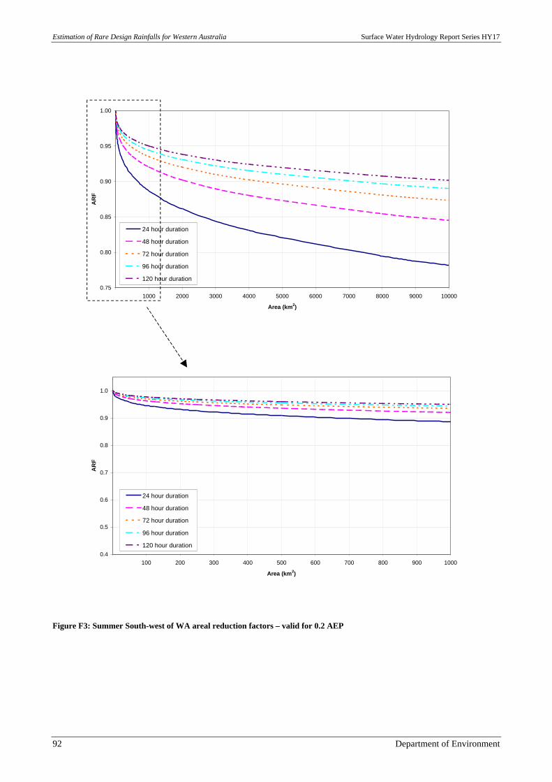
Estimation of Rare Design Rainfalls for Western Australia Surface Water Hydrology Report Series HY17
92 Department of Environment
South-west of WA 0.2 AEP
0.75
0.80
0.85
0.90
0.95
1.00
0 1000 2000 3000 4000 5000 6000 7000 8000 9000 10000
Area (km2)
AR
F
24 hour duration
48 hour duration
72 hour duration
96 hour duration
120 hour duration
0.4
0.5
0.6
0.7
0.8
0.9
1.0
0 100 200 300 400 500 600 700 800 900 1000
Area (km2)
AR
F
24 hour duration
48 hour duration
72 hour duration
96 hour duration
120 hour duration
Figure F3: Summer South-west of WA areal reduction factors – valid for 0.2 AEP
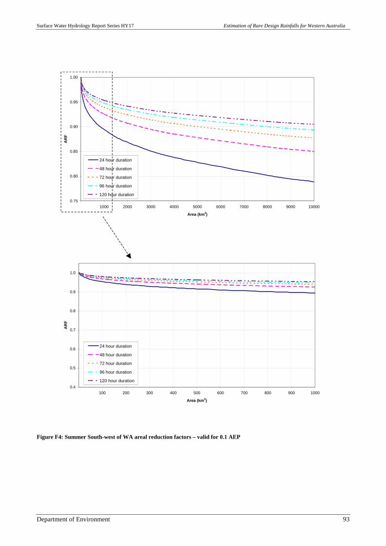
Surface Water Hydrology Report Series HY17 Estimation of Rare Design Rainfalls for Western Australia
Department of Environment 93
South-west of WA 0.1 AEP
0.75
0.80
0.85
0.90
0.95
1.00
0 1000 2000 3000 4000 5000 6000 7000 8000 9000 10000
Area (km2)
AR
F
24 hour duration
48 hour duration
72 hour duration
96 hour duration
120 hour duration
0.4
0.5
0.6
0.7
0.8
0.9
1.0
0 100 200 300 400 500 600 700 800 900 1000
Area (km2)
AR
F
24 hour duration
48 hour duration
72 hour duration
96 hour duration
120 hour duration
Figure F4: Summer South-west of WA areal reduction factors – valid for 0.1 AEP
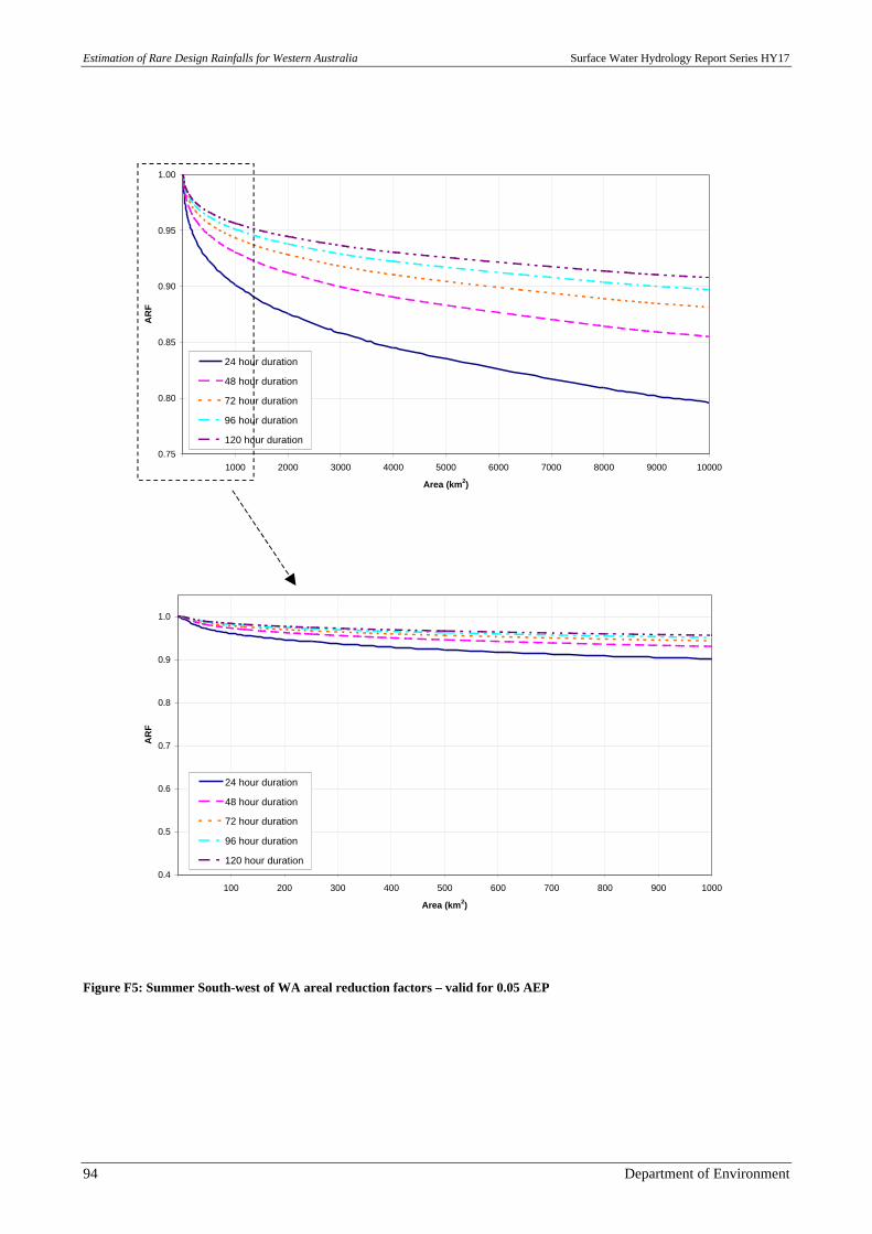
Estimation of Rare Design Rainfalls for Western Australia Surface Water Hydrology Report Series HY17
94 Department of Environment
South-west of WA 0.05 AEP
0.75
0.80
0.85
0.90
0.95
1.00
0 1000 2000 3000 4000 5000 6000 7000 8000 9000 10000
Area (km2)
AR
F
24 hour duration
48 hour duration
72 hour duration
96 hour duration
120 hour duration
0.4
0.5
0.6
0.7
0.8
0.9
1.0
0 100 200 300 400 500 600 700 800 900 1000
Area (km2)
AR
F
24 hour duration
48 hour duration
72 hour duration
96 hour duration
120 hour duration
Figure F5: Summer South-west of WA areal reduction factors – valid for 0.05 AEP
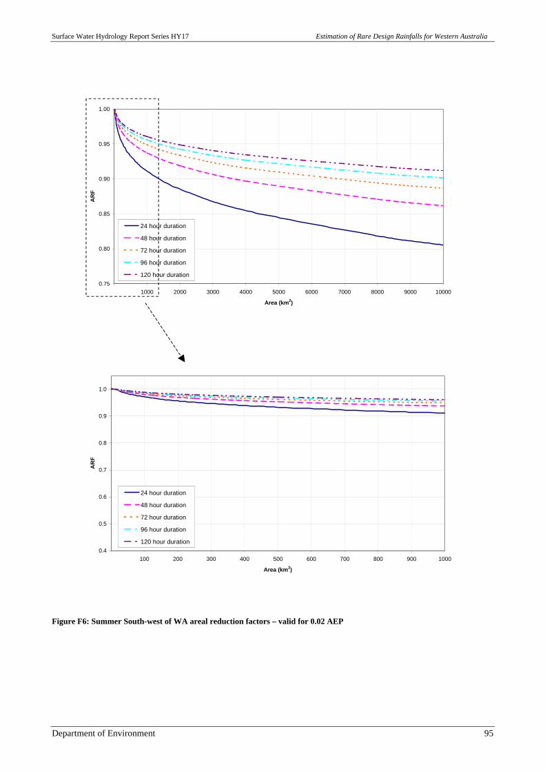
Surface Water Hydrology Report Series HY17 Estimation of Rare Design Rainfalls for Western Australia
Department of Environment 95
South-west of WA 0.02 AEP
0.75
0.80
0.85
0.90
0.95
1.00
0 1000 2000 3000 4000 5000 6000 7000 8000 9000 10000
Area (km2)
AR
F
24 hour duration
48 hour duration
72 hour duration
96 hour duration
120 hour duration
0.4
0.5
0.6
0.7
0.8
0.9
1.0
0 100 200 300 400 500 600 700 800 900 1000
Area (km2)
AR
F
24 hour duration
48 hour duration
72 hour duration
96 hour duration
120 hour duration
Figure F6: Summer South-west of WA areal reduction factors – valid for 0.02 AEP
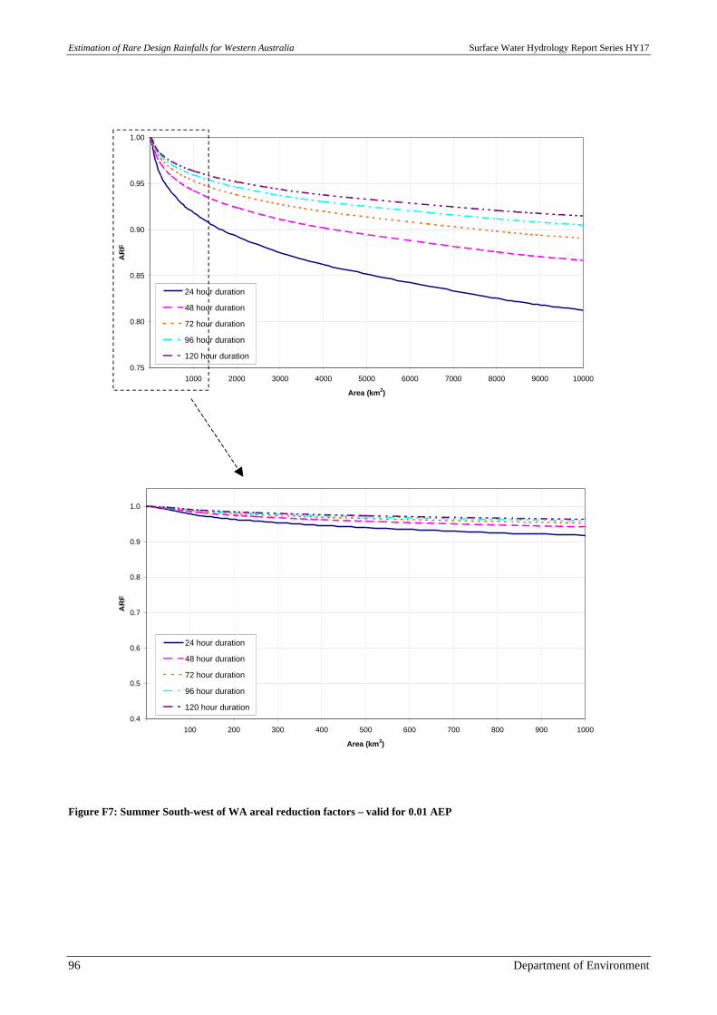
Estimation of Rare Design Rainfalls for Western Australia Surface Water Hydrology Report Series HY17
96 Department of Environment
0.75
0.80
0.85
0.90
0.95
1.00
0 1000 2000 3000 4000 5000 6000 7000 8000 9000 10000
Area (km2)
AR
F
24 hour duration
48 hour duration
72 hour duration
96 hour duration
120 hour duration
0.4
0.5
0.6
0.7
0.8
0.9
1.0
0 100 200 300 400 500 600 700 800 900 1000
Area (km2)
AR
F
24 hour duration
48 hour duration
72 hour duration
96 hour duration
120 hour duration
Figure F7: Summer South-west of WA areal reduction factors – valid for 0.01 AEP
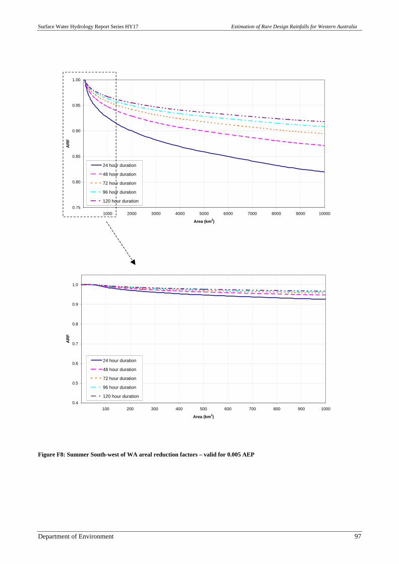
Surface Water Hydrology Report Series HY17 Estimation of Rare Design Rainfalls for Western Australia
Department of Environment 97
South-west of WA 0.005 AEP
0.75
0.80
0.85
0.90
0.95
1.00
0 1000 2000 3000 4000 5000 6000 7000 8000 9000 10000
Area (km2)
AR
F
24 hour duration
48 hour duration
72 hour duration
96 hour duration
120 hour duration
0.4
0.5
0.6
0.7
0.8
0.9
1.0
0 100 200 300 400 500 600 700 800 900 1000
Area (km2)
AR
F
24 hour duration
48 hour duration
72 hour duration
96 hour duration
120 hour duration
Figure F8: Summer South-west of WA areal reduction factors – valid for 0.005 AEP
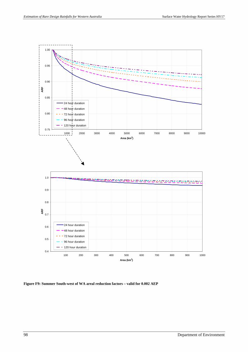
Estimation of Rare Design Rainfalls for Western Australia Surface Water Hydrology Report Series HY17
98 Department of Environment
South-west of WA 0.002 AEP
0.75
0.80
0.85
0.90
0.95
1.00
0 1000 2000 3000 4000 5000 6000 7000 8000 9000 10000
Area (km2)
AR
F
24 hour duration
48 hour duration
72 hour duration
96 hour duration
120 hour duration
0.4
0.5
0.6
0.7
0.8
0.9
1.0
0 100 200 300 400 500 600 700 800 900 1000
Area (km2)
AR
F
24 hour duration
48 hour duration
72 hour duration
96 hour duration
120 hour duration
Figure F9: Summer South-west of WA areal reduction factors – valid for 0.002 AEP
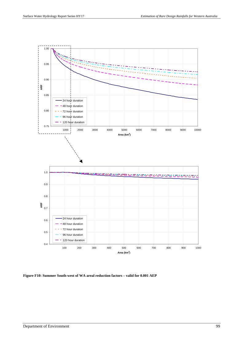
Surface Water Hydrology Report Series HY17 Estimation of Rare Design Rainfalls for Western Australia
Department of Environment 99
South-west of WA 0.001 AEP
0.75
0.80
0.85
0.90
0.95
1.00
0 1000 2000 3000 4000 5000 6000 7000 8000 9000 10000
Area (km2)
AR
F
24 hour duration
48 hour duration
72 hour duration
96 hour duration
120 hour duration
0.4
0.5
0.6
0.7
0.8
0.9
1.0
0 100 200 300 400 500 600 700 800 900 1000
Area (km2)
AR
F
24 hour duration
48 hour duration
72 hour duration
96 hour duration
120 hour duration
Figure F10: Summer South-west of WA areal reduction factors – valid for 0.001 AEP
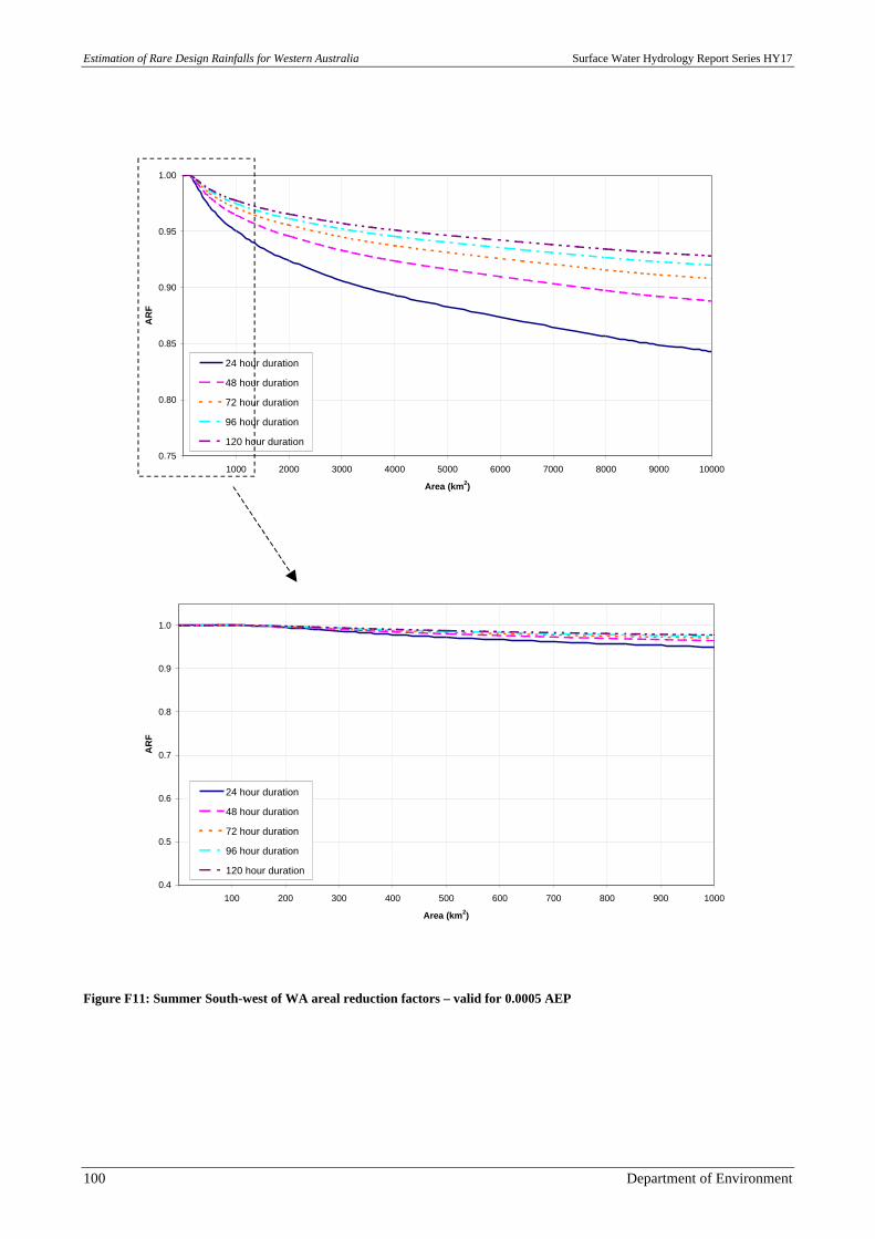
Estimation of Rare Design Rainfalls for Western Australia Surface Water Hydrology Report Series HY17
100 Department of Environment
South-west of WA 0.0005 AEP
0.75
0.80
0.85
0.90
0.95
1.00
0 1000 2000 3000 4000 5000 6000 7000 8000 9000 10000
Area (km2)
AR
F
24 hour duration
48 hour duration
72 hour duration
96 hour duration
120 hour duration
0.4
0.5
0.6
0.7
0.8
0.9
1.0
0 100 200 300 400 500 600 700 800 900 1000
Area (km2)
AR
F
24 hour duration
48 hour duration
72 hour duration
96 hour duration
120 hour duration
Figure F11: Summer South-west of WA areal reduction factors – valid for 0.0005 AEP
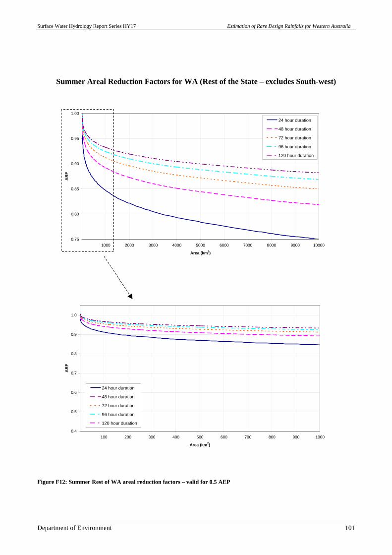
Surface Water Hydrology Report Series HY17 Estimation of Rare Design Rainfalls for Western Australia
Department of Environment 101
Summer Areal Reduction Factors for WA (Rest of the State – excludes South-west)
0.75
0.80
0.85
0.90
0.95
1.00
0 1000 2000 3000 4000 5000 6000 7000 8000 9000 10000
Area (km2)
AR
F
24 hour duration
48 hour duration
72 hour duration
96 hour duration
120 hour duration
0.4
0.5
0.6
0.7
0.8
0.9
1.0
0 100 200 300 400 500 600 700 800 900 1000
Area (km2)
AR
F
24 hour duration
48 hour duration
72 hour duration
96 hour duration
120 hour duration
Figure F12: Summer Rest of WA areal reduction factors – valid for 0.5 AEP
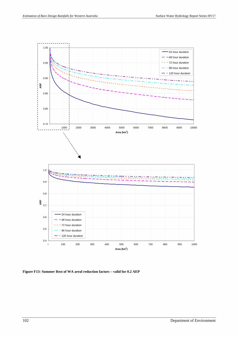
Estimation of Rare Design Rainfalls for Western Australia Surface Water Hydrology Report Series HY17
102 Department of Environment
Rest of WA 0.2 AEP
0.75
0.80
0.85
0.90
0.95
1.00
0 1000 2000 3000 4000 5000 6000 7000 8000 9000 10000
Area (km2)
AR
F
24 hour duration
48 hour duration
72 hour duration
96 hour duration
120 hour duration
0.4
0.5
0.6
0.7
0.8
0.9
1.0
0 100 200 300 400 500 600 700 800 900 1000
Area (km2)
AR
F
24 hour duration
48 hour duration
72 hour duration
96 hour duration
120 hour duration
Figure F13: Summer Rest of WA areal reduction factors – valid for 0.2 AEP
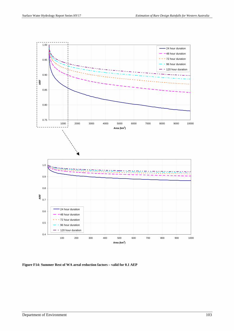
Surface Water Hydrology Report Series HY17 Estimation of Rare Design Rainfalls for Western Australia
Department of Environment 103
0.75
0.80
0.85
0.90
0.95
1.00
0 1000 2000 3000 4000 5000 6000 7000 8000 9000 10000
Area (km2)
AR
F
24 hour duration
48 hour duration
72 hour duration
96 hour duration
120 hour duration
0.4
0.5
0.6
0.7
0.8
0.9
1.0
0 100 200 300 400 500 600 700 800 900 1000
Area (km2)
AR
F
24 hour duration
48 hour duration
72 hour duration
96 hour duration
120 hour duration
Figure F14: Summer Rest of WA areal reduction factors – valid for 0.1 AEP
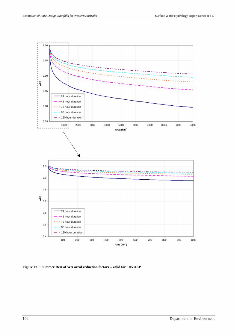
Estimation of Rare Design Rainfalls for Western Australia Surface Water Hydrology Report Series HY17
104 Department of Environment
0.75
0.80
0.85
0.90
0.95
1.00
0 1000 2000 3000 4000 5000 6000 7000 8000 9000 10000
Area (km2)
AR
F
24 hour duration
48 hour duration
72 hour duration
96 hour duration
120 hour duration
0.4
0.5
0.6
0.7
0.8
0.9
1.0
0 100 200 300 400 500 600 700 800 900 1000
Area (km2)
AR
F
24 hour duration
48 hour duration
72 hour duration
96 hour duration
120 hour duration
Figure F15: Summer Rest of WA areal reduction factors – valid for 0.05 AEP

Surface Water Hydrology Report Series HY17 Estimation of Rare Design Rainfalls for Western Australia
Department of Environment 105
0.75
0.80
0.85
0.90
0.95
1.00
0 1000 2000 3000 4000 5000 6000 7000 8000 9000 10000
Area (km2)
AR
F
24 hour duration
48 hour duration
72 hour duration
96 hour duration
120 hour duration
0.4
0.5
0.6
0.7
0.8
0.9
1.0
0 100 200 300 400 500 600 700 800 900 1000
Area (km2)
AR
F
24 hour duration
48 hour duration
72 hour duration
96 hour duration
120 hour duration
Figure F16: Summer Rest of WA areal reduction factors – valid for 0.02 AEP
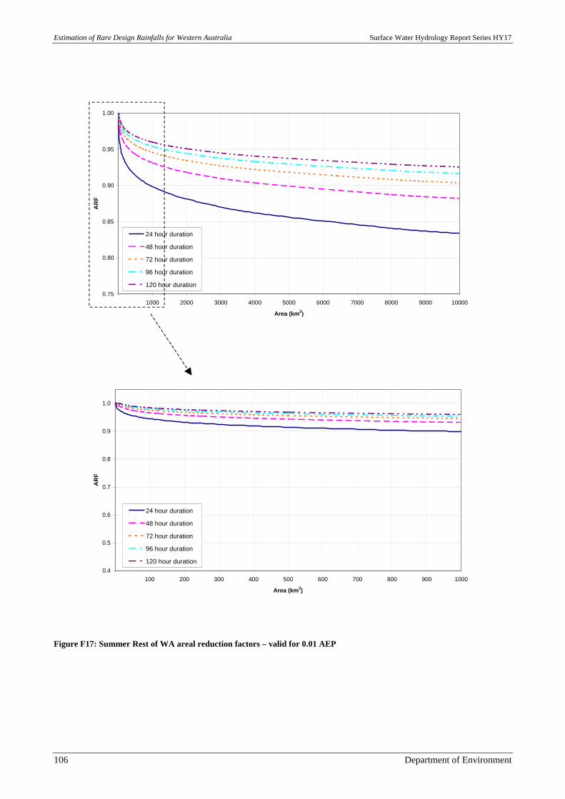
Estimation of Rare Design Rainfalls for Western Australia Surface Water Hydrology Report Series HY17
106 Department of Environment
Rest of WA 0.01 AEP
0.75
0.80
0.85
0.90
0.95
1.00
0 1000 2000 3000 4000 5000 6000 7000 8000 9000 10000
Area (km2)
AR
F
24 hour duration
48 hour duration
72 hour duration
96 hour duration
120 hour duration
0.4
0.5
0.6
0.7
0.8
0.9
1.0
0 100 200 300 400 500 600 700 800 900 1000
Area (km2)
AR
F
24 hour duration
48 hour duration
72 hour duration
96 hour duration
120 hour duration
Figure F17: Summer Rest of WA areal reduction factors – valid for 0.01 AEP
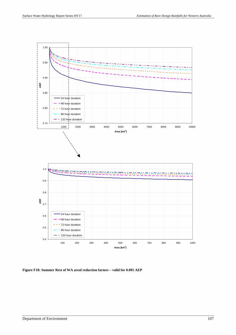
Surface Water Hydrology Report Series HY17 Estimation of Rare Design Rainfalls for Western Australia
Department of Environment 107
Rest of WA 0.005 AEP
0.75
0.80
0.85
0.90
0.95
1.00
0 1000 2000 3000 4000 5000 6000 7000 8000 9000 10000
Area (km2)
AR
F
24 hour duration
48 hour duration
72 hour duration
96 hour duration
120 hour duration
0.4
0.5
0.6
0.7
0.8
0.9
1.0
0 100 200 300 400 500 600 700 800 900 1000
Area (km2)
AR
F
24 hour duration
48 hour duration
72 hour duration
96 hour duration
120 hour duration
Figure F18: Summer Rest of WA areal reduction factors – valid for 0.005 AEP
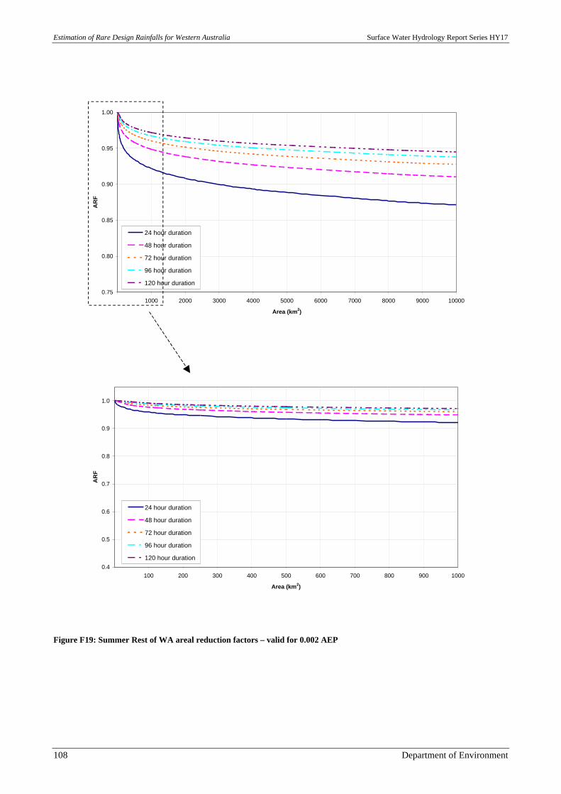
Estimation of Rare Design Rainfalls for Western Australia Surface Water Hydrology Report Series HY17
108 Department of Environment
Rest of WA 0.002 AEP
0.75
0.80
0.85
0.90
0.95
1.00
0 1000 2000 3000 4000 5000 6000 7000 8000 9000 10000
Area (km2)
AR
F
24 hour duration
48 hour duration
72 hour duration
96 hour duration
120 hour duration
0.4
0.5
0.6
0.7
0.8
0.9
1.0
0 100 200 300 400 500 600 700 800 900 1000
Area (km2)
AR
F
24 hour duration
48 hour duration
72 hour duration
96 hour duration
120 hour duration
Figure F19: Summer Rest of WA areal reduction factors – valid for 0.002 AEP
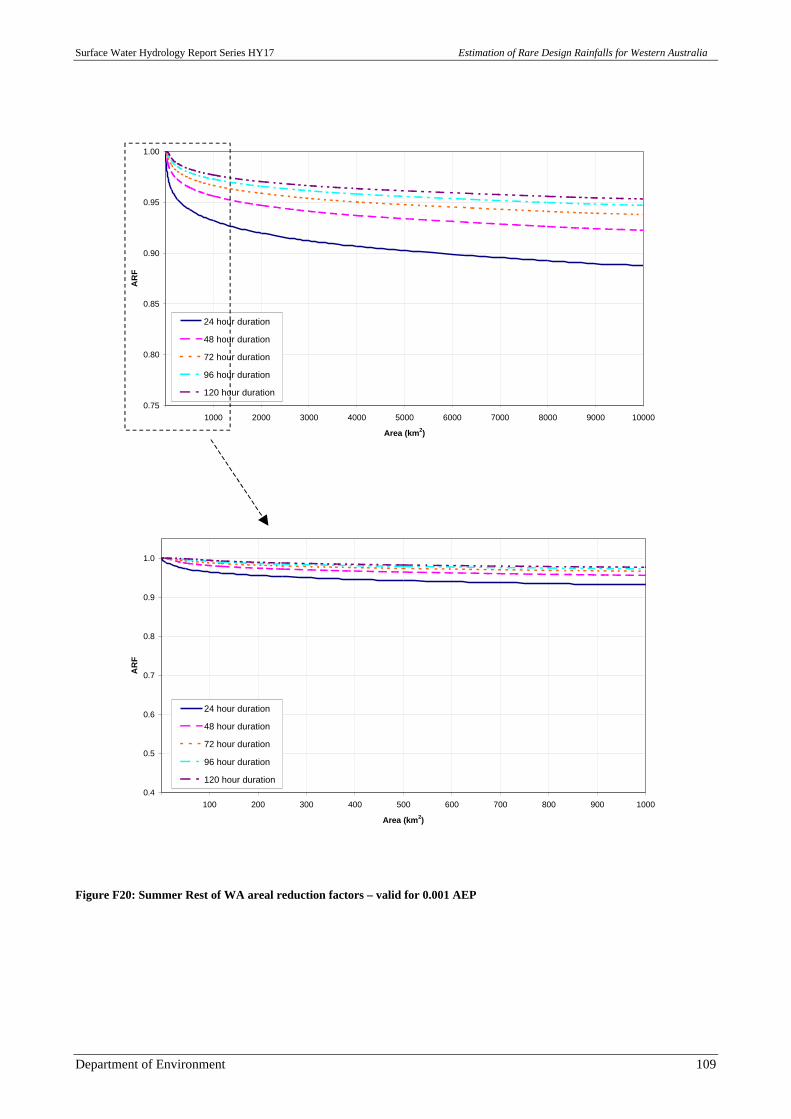
Surface Water Hydrology Report Series HY17 Estimation of Rare Design Rainfalls for Western Australia
Department of Environment 109
0.75
0.80
0.85
0.90
0.95
1.00
0 1000 2000 3000 4000 5000 6000 7000 8000 9000 10000
Area (km2)
AR
F
24 hour duration
48 hour duration
72 hour duration
96 hour duration
120 hour duration
0.4
0.5
0.6
0.7
0.8
0.9
1.0
0 100 200 300 400 500 600 700 800 900 1000
Area (km2)
AR
F
24 hour duration
48 hour duration
72 hour duration
96 hour duration
120 hour duration
Figure F20: Summer Rest of WA areal reduction factors – valid for 0.001 AEP
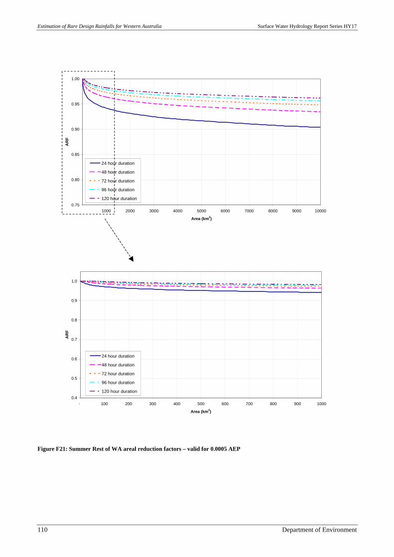
Estimation of Rare Design Rainfalls for Western Australia Surface Water Hydrology Report Series HY17
110 Department of Environment
Rest of WA 0.0005 AEP
0.75
0.80
0.85
0.90
0.95
1.00
0 1000 2000 3000 4000 5000 6000 7000 8000 9000 10000
Area (km2)
AR
F
24 hour duration
48 hour duration
72 hour duration
96 hour duration
120 hour duration
0.4
0.5
0.6
0.7
0.8
0.9
1.0
0 100 200 300 400 500 600 700 800 900 1000
Area (km2)
AR
F
24 hour duration
48 hour duration
72 hour duration
96 hour duration
120 hour duration
Figure F21: Summer Rest of WA areal reduction factors – valid for 0.0005 AEP
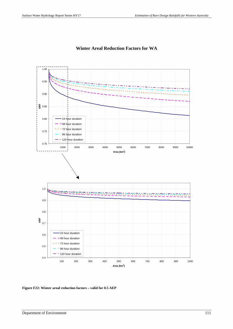
Surface Water Hydrology Report Series HY17 Estimation of Rare Design Rainfalls for Western Australia
Department of Environment 111
Winter Areal Reduction Factors for WA
0.5 AEP
0.70
0.75
0.80
0.85
0.90
0.95
1.00
0 1000 2000 3000 4000 5000 6000 7000 8000 9000 10000
Area (km2)
AR
F
24 hour duration
48 hour duration
72 hour duration
96 hour duration
120 hour duration
0.5 AEP
0.4
0.5
0.6
0.7
0.8
0.9
1.0
0 100 200 300 400 500 600 700 800 900 1000
Area (km2)
AR
F
24 hour duration
48 hour duration
72 hour duration
96 hour duration
120 hour duration
Figure F22: Winter areal reduction factors – valid for 0.5 AEP
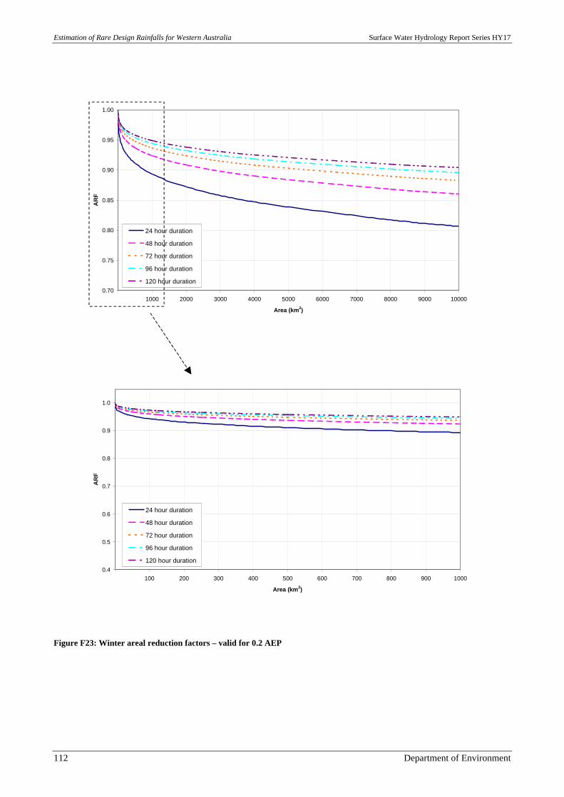
Estimation of Rare Design Rainfalls for Western Australia Surface Water Hydrology Report Series HY17
112 Department of Environment
0.70
0.75
0.80
0.85
0.90
0.95
1.00
0 1000 2000 3000 4000 5000 6000 7000 8000 9000 10000
Area (km2)
AR
F
24 hour duration
48 hour duration
72 hour duration
96 hour duration
120 hour duration
0.2 AEP
0.4
0.5
0.6
0.7
0.8
0.9
1.0
0 100 200 300 400 500 600 700 800 900 1000
Area (km2)
AR
F
24 hour duration
48 hour duration
72 hour duration
96 hour duration
120 hour duration
Figure F23: Winter areal reduction factors – valid for 0.2 AEP
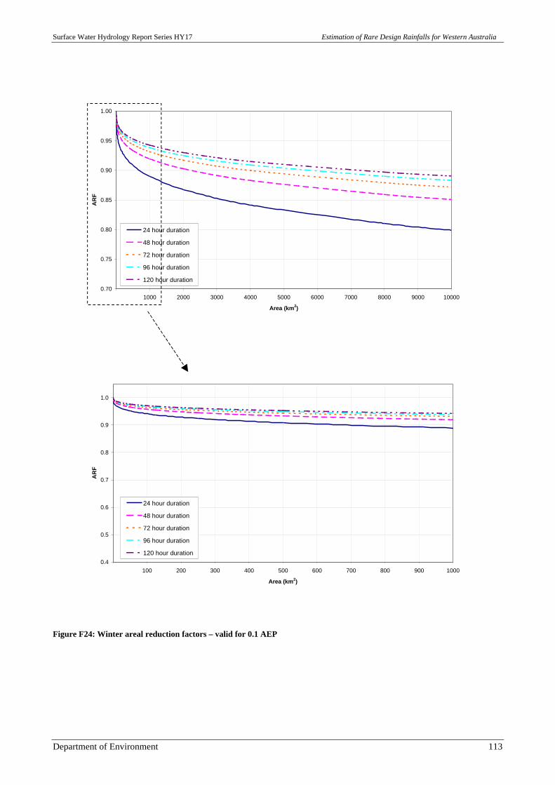
Surface Water Hydrology Report Series HY17 Estimation of Rare Design Rainfalls for Western Australia
Department of Environment 113
0.1 AEP
0.70
0.75
0.80
0.85
0.90
0.95
1.00
0 1000 2000 3000 4000 5000 6000 7000 8000 9000 10000
Area (km2)
AR
F
24 hour duration
48 hour duration
72 hour duration
96 hour duration
120 hour duration
0.4
0.5
0.6
0.7
0.8
0.9
1.0
0 100 200 300 400 500 600 700 800 900 1000
Area (km2)
AR
F
24 hour duration
48 hour duration
72 hour duration
96 hour duration
120 hour duration
Figure F24: Winter areal reduction factors – valid for 0.1 AEP
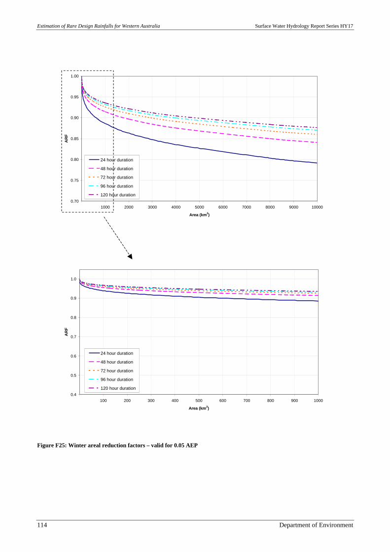
Estimation of Rare Design Rainfalls for Western Australia Surface Water Hydrology Report Series HY17
114 Department of Environment
0.70
0.75
0.80
0.85
0.90
0.95
1.00
0 1000 2000 3000 4000 5000 6000 7000 8000 9000 10000
Area (km2)
AR
F
24 hour duration
48 hour duration
72 hour duration
96 hour duration
120 hour duration
0.05 AEP
0.4
0.5
0.6
0.7
0.8
0.9
1.0
0 100 200 300 400 500 600 700 800 900 1000
Area (km2)
AR
F
24 hour duration
48 hour duration
72 hour duration
96 hour duration
120 hour duration
Figure F25: Winter areal reduction factors – valid for 0.05 AEP
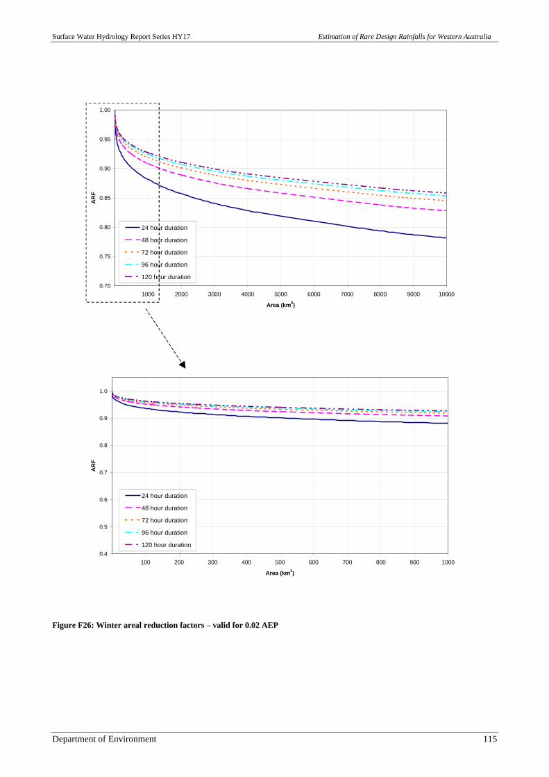
Surface Water Hydrology Report Series HY17 Estimation of Rare Design Rainfalls for Western Australia
Department of Environment 115
0.02 AEP
0.70
0.75
0.80
0.85
0.90
0.95
1.00
0 1000 2000 3000 4000 5000 6000 7000 8000 9000 10000
Area (km2)
AR
F
24 hour duration
48 hour duration
72 hour duration
96 hour duration
120 hour duration
0.4
0.5
0.6
0.7
0.8
0.9
1.0
0 100 200 300 400 500 600 700 800 900 1000
Area (km2)
AR
F
24 hour duration
48 hour duration
72 hour duration
96 hour duration
120 hour duration
Figure F26: Winter areal reduction factors – valid for 0.02 AEP
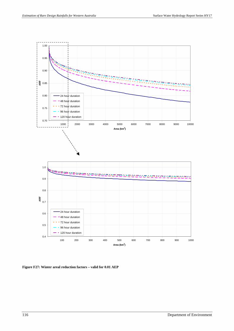
Estimation of Rare Design Rainfalls for Western Australia Surface Water Hydrology Report Series HY17
116 Department of Environment
0.70
0.75
0.80
0.85
0.90
0.95
1.00
0 1000 2000 3000 4000 5000 6000 7000 8000 9000 10000
Area (km2)
AR
F
24 hour duration
48 hour duration
72 hour duration
96 hour duration
120 hour duration
0.01 AEP
0.4
0.5
0.6
0.7
0.8
0.9
1.0
0 100 200 300 400 500 600 700 800 900 1000
Area (km2)
AR
F
24 hour duration
48 hour duration
72 hour duration
96 hour duration
120 hour duration
Figure F27: Winter areal reduction factors – valid for 0.01 AEP
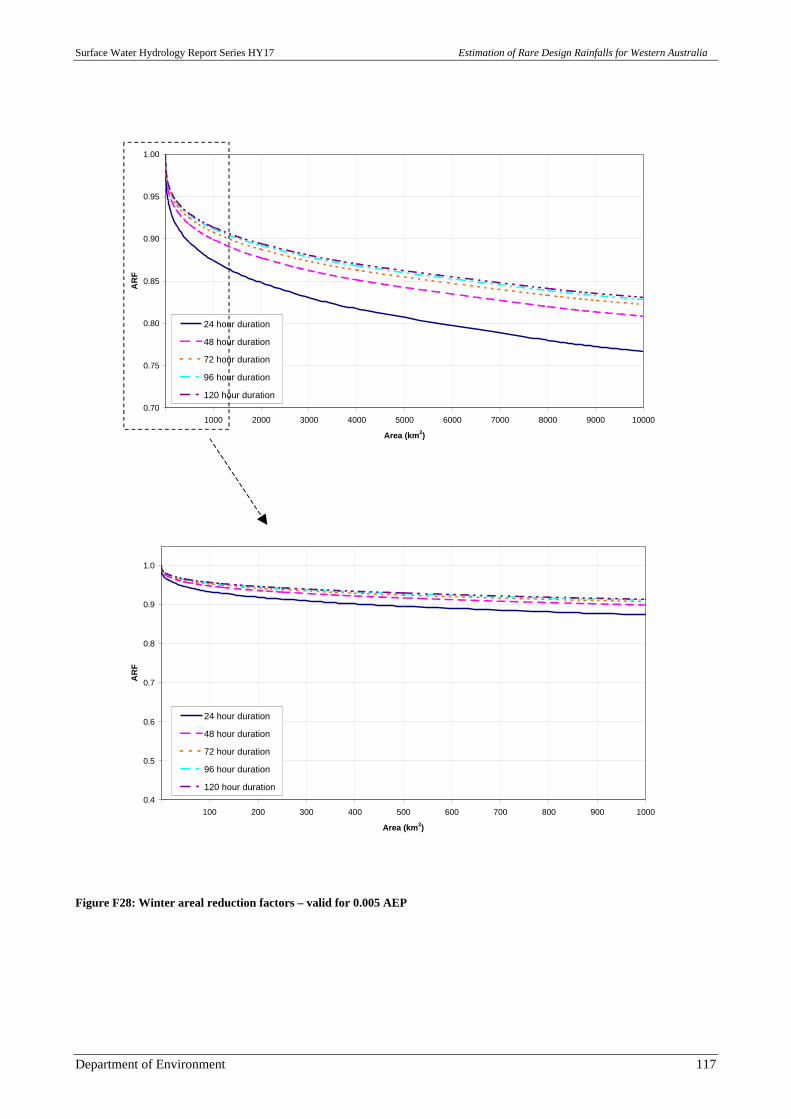
Surface Water Hydrology Report Series HY17 Estimation of Rare Design Rainfalls for Western Australia
Department of Environment 117
0.70
0.75
0.80
0.85
0.90
0.95
1.00
0 1000 2000 3000 4000 5000 6000 7000 8000 9000 10000
Area (km2)
AR
F
24 hour duration
48 hour duration
72 hour duration
96 hour duration
120 hour duration
0.005 AEP
0.4
0.5
0.6
0.7
0.8
0.9
1.0
0 100 200 300 400 500 600 700 800 900 1000
Area (km2)
AR
F
24 hour duration
48 hour duration
72 hour duration
96 hour duration
120 hour duration
Figure F28: Winter areal reduction factors – valid for 0.005 AEP
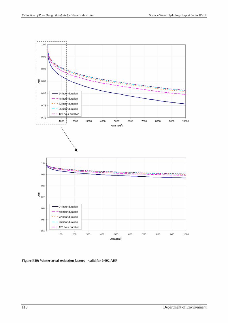
Estimation of Rare Design Rainfalls for Western Australia Surface Water Hydrology Report Series HY17
118 Department of Environment
0.70
0.75
0.80
0.85
0.90
0.95
1.00
0 1000 2000 3000 4000 5000 6000 7000 8000 9000 10000
Area (km2)
AR
F
24 hour duration
48 hour duration
72 hour duration
96 hour duration
120 hour duration
0.002 AEP
0.4
0.5
0.6
0.7
0.8
0.9
1.0
0 100 200 300 400 500 600 700 800 900 1000
Area (km2)
AR
F
24 hour duration
48 hour duration
72 hour duration
96 hour duration
120 hour duration
Figure F29: Winter areal reduction factors – valid for 0.002 AEP
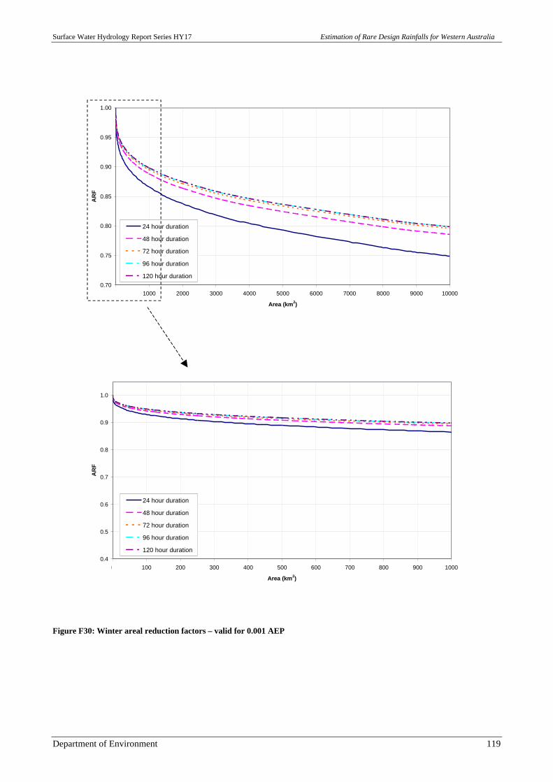
Surface Water Hydrology Report Series HY17 Estimation of Rare Design Rainfalls for Western Australia
Department of Environment 119
0.70
0.75
0.80
0.85
0.90
0.95
1.00
0 1000 2000 3000 4000 5000 6000 7000 8000 9000 10000
Area (km2)
AR
F
24 hour duration
48 hour duration
72 hour duration
96 hour duration
120 hour duration
0.001 AEP
0.4
0.5
0.6
0.7
0.8
0.9
1.0
0 100 200 300 400 500 600 700 800 900 1000
Area (km2)
AR
F
24 hour duration
48 hour duration
72 hour duration
96 hour duration
120 hour duration
Figure F30: Winter areal reduction factors – valid for 0.001 AEP
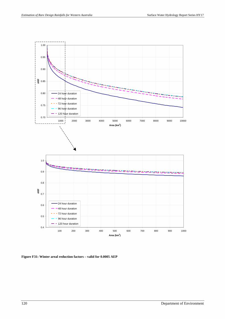
Estimation of Rare Design Rainfalls for Western Australia Surface Water Hydrology Report Series HY17
120 Department of Environment
0.0005 AEP
0.70
0.75
0.80
0.85
0.90
0.95
1.00
0 1000 2000 3000 4000 5000 6000 7000 8000 9000 10000
Area (km2)
AR
F
24 hour duration
48 hour duration
72 hour duration
96 hour duration
120 hour duration
0.4
0.5
0.6
0.7
0.8
0.9
1.0
0 100 200 300 400 500 600 700 800 900 1000
Area (km2)
AR
F
24 hour duration
48 hour duration
72 hour duration
96 hour duration
120 hour duration
Figure F31: Winter areal reduction factors – valid for 0.0005 AEP

Surface Water Hydrology Report Series HY17 Estimation of Rare Design Rainfalls for Western Australia
Publication feedback form
The Department of Environment welcomes feedback to help us improve thequality and effectiveness of our publications. Your assistance in completingthis form would be greatly appreciated.
Please consider each question carefully and rate them on a 1 to 5 scale,where 1 is poor and 5 is excellent (please circle the appropriate number).
How did you rate the quality of information?
1 2 3 4 5
How did you rate the design and presentation of this publication?
1 2 3 4 5
How can it be improved?
.....................................................................................................................
How effective did you find the tables and figures in communicating the data?
1 2 3 4 5
How can they be improved?
.....................................................................................................................
.....................................................................................................................
.....................................................................................................................
If you would like to see this publication in other formats, please specify. (e.g. CD)
.....................................................................................................................
Please cut along the dotted line on the left and return your completed response to:
Publications CoordinatorDepartment of EnvironmentLevel 2, Hyatt Centre3 Plain StreetEast Perth WA 6004Fax: (08) 9278 0639