Estimation of Markov Chain via Rank-constrained Likelihood

Estimation of Markov Chain via Rank-Constrained Likelihood

Xudong Li 1 Mengdi Wang 1 Anru Zhang 2

AbstractThis paper studies the estimation of low-rankMarkov chains from empirical trajectories. Wepropose a non-convex estimator based on rank-constrained likelihood maximization. Statisti-cal upper bounds are provided for the Kullback-Leiber divergence and the `2 risk between theestimator and the true transition matrix. The es-timator reveals a compressed state space of theMarkov chain. We also develop a novel DC (dif-ference of convex function) programming algo-rithm to tackle the rank-constrained non-smoothoptimization problem. Convergence results areestablished. Experiments show that the proposedestimator achieves better empirical performancethan other popular approaches.

1. IntroductionIn scientific studies, engineering systems, and social envi-ronments, one often has to interact with complex processeswith uncertainties, collect data, and learn to make predic-tions and decisions. A critical question is how to model theunknown random process from data. To answer this ques-tion, we particularly focus on discrete Markov chains witha finite but potentially huge state space. Suppose we aregiven a sequence of observations generated by an unknownMarkov process. The true transition matrix is unknown, andthe physical states of the system and its law of transition ishidden under massive noisy observations. We are interestedin the estimation and state compression of Markov pro-cesses, i.e., to identify compact representations of the statespace and recover a reduced-dimensional Markov model.

To be more specific, we focus on the estimation of a class

1Department of Operations Research and FinancialEngineering, Princeton University, Sherrerd Hall, Prince-ton, NJ 08544 2Department of Statistics, University ofWisconsin-Madison, Madison, WI 53706. Correspon-dence to: Xudong Li <[email protected]>, MengdiWang <[email protected]>, Anru Zhang <[email protected]>.

Proceedings of the 35 th International Conference on MachineLearning, Stockholm, Sweden, PMLR 80, 2018. Copyright 2018by the author(s).

of Markov chains with low-rank transition matrices in thispaper. Low-rankness is ubiquitous in practice. For exam-ple, the random walk of a taxi turns out to correspond toa nearly low-rank Markov chain. Each taxi trip can beviewed as a sample transition of a city-wide random walkthat characterizes the traffic dynamics. For another exam-ple, control and reinforcement learning, which are typicallymodeled as Markov decision processes, suffer from thecurse of dimensionality (Sutton & Barto, 1998). It is ofvital interest to identify the compressed representation ofthe “state” of game, in order to reduce the dimensionalityof policy and value functions. Multiple efforts show that aslong as a reduced model or a compact state representationis given, one can solve high-dimensional control problemsin sample-efficient ways; see (Singh et al., 1995; Van Roy,2006; Malek et al., 2014) for examples.

The low-rank Markov chain is a basic model for analyzingdata generated by stochastic processes. It is closely relatedto a variety of latent-variable models, including Markov pro-cess with rich observations (Azizzadenesheli et al., 2016),state aggregation models (Singh et al., 1995) and hiddenMarkov models (Hsu et al., 2012). Low-rankness of Markovchains can be used to recover network partition under somelumpability assumption (E et al., 2008). In particular, low-rank Markov chain can be viewed as a special form ofhidden Markov model where the observations contain allthe information of the hidden states.

In this article, we propose a rank-constrained maximum like-lihood approach for transition matrix estimation from em-pirical trajectories. The statistical guarantees is developedfor the proposed estimator. Especially, the upper bounds forthe Kullback-Leibler (KL) divergence between the estima-tor and the true transition matrix as well as the `2 risk areestablished. We further provide a minimax lower bound toshow that the proposed estimator is near rate-optimal withina class of low-rank Markov chains. A related recent work(Zhang & Wang, 2017) considered the low-rank estimationby a spectral method and established upper bound for thetotal variation. Compared to the existing results, our max-imum likelihood estimator and the KL-divergence boundsappear to be the first ones of this type.

The proposed estimator requires solving an optimizationproblem with both rank and polyhedral constraints. Due tothe presence of non-convex rank constraint, the optimiza-

arX

iv:1

804.

0079

5v2

[st

at.M

L]

19

Jul 2

018

Estimation of Markov Chain via Rank-constrained Likelihood

tion problem is difficult – there is no efficient approach thatdirectly applies to such a non-convex problem, to the best ofour knowledge. In this paper, we use a penalty approach torelax the rank constraint and transform the original probleminto a DC (difference of convex functions) programming one.Furthermore, we develop a corresponding DC algorithm tosolve the problem. The algorithm proceeds by solving asequence of inner subproblems, for which we develop anefficient subroutine based on multi-block alternating direc-tion method of multipliers (ADMM). As a byproduct ofthis research, we develop a new class of DC algorithmsand a unified convergence analysis for solving non-convexnon-smooth problems.

Finally, the performance of the proposed estimator and al-gorithm is verified through simulation studies.

2. Related literaturesModel reduction for complicated systems has a long his-tory that traces back to variable-resolution dynamic pro-gramming (Moore, 1991) and state aggregation for decisionprocess (Sutton & Barto, 1998). In particular, (Deng et al.,2011; Deng & Huang, 2012) considered low-rank reductionof Markov models with explicitly known transition proba-bility matrix, but not the estimation of the reduced models.

Low-rank models and spectral methods have been provedpowerful in extracting features from high-dimensional data,with numerous applications including network analysis (Eet al., 2008), community detection (Newman, 2013), ranking(Negahban et al., 2016), product recommendation (Kesha-van et al., 2010) and many more. Estimation of hiddenMarkov models is related to spectral matrix/tensor decom-position, which has been considered in (Hsu et al., 2012).Later, (Anandkumar et al., 2014) studied a more generaltensor-decomposition-based spectral approach, which canbe applied to a variety of latent variable models includinghidden Markov models. (Huang et al., 2016) consideredthe estimation of a rank-two probabilistic matrix from a fewnumber of independent samples. Estimation of low-rankMarkov chain was considered for the first time in (Zhang &Wang, 2017). Particularly, a spectral method via truncatedsingular value decomposition was introduced and the upperand lower error bounds in total variation were established.(Yang et al., 2017) developed an online stochastic gradientmethod for computing the leading singular space of a transi-tion matrix from random walk data. The online stochasticapproximation algorithms were also analyzed recently in (Liet al., 2017; 2018) for principal component estimation. Theestimation of discrete distributions in the form of vectors isanother line of related research, where the procedure and es-timation risk has been considered in both classic and recentliterature (Steinhaus, 1957; Lehmann & Casella, 2006; Hanet al., 2015).

Form the perspective of optimization, DC programming is abackbone in handling the rank-constrained problem. First in-troduced by (Pham Dinh & Le Thi, 1997), the DC algorithmhas become a prominent tool for handling a class of noncon-vex optimization problems (see also (Pham Dinh & Le Thi,2005; Le Thi et al., 2012; 2017; Le Thi & Pham Dinh,2018)). In particular, (Van Dinh et al., 2015; Wen et al.,2017) considered the majorized indefinite-proximal DC al-gorithm, which is closely related to the optimization meth-ods in this paper. However, both (Van Dinh et al., 2015; Wenet al., 2017) used the majorization technique with restrictedchoices of majorants, neither considered the introductionof the indefinite proximal terms, and (Wen et al., 2017)further requires the smooth part in the objective to be con-vex. A more flexible algorithmic framework and a unifiedconvergence analysis is provided in Section 5.4.

3. Low-rank Markov chains and latentvariable models

Consider a discrete-time Markov chain on p statess1, . . . , sp with transition matrix P ∈ <p×p. Then Psatisfies Pij = P (sj |si), 0 ≤ Pij ≤ 1, and

∑pj=1 Pij = 1

for 1 ≤ i, j ≤ p. Let µ be the corresponding stationarydistribution. Suppose rank(P) = r. Motivated by the ex-amples that we will discuss below, we focus on the casewhere r p, i.e., the rank of P is significantly smaller thanthe total number of states.

The first example of low-rank Markov chain in reduced-order models is the state aggregation – a basic model fordescribing complicated systems (Bertsekas, 1995; Bertsekas& Tsitsiklis, 1995). If a process admits an inherent stateaggregation structure, its states can be clustered into a smallnumber of disjoint subsets, such that states from the samecluster have identical transition distribution. We say that aMarkov chain is state aggregatable if there exists a partitionS1,S2, . . . ,Sr such that

P (· | s) = P (· | s′), ∀s, s′ ∈ Si, i ∈ [r].

It can be shown that the state aggregation yields a specialfactorization of transition matrix. Particularly, there existsU,V ∈ <p×r such that

P = UV>,

where each row of U has all 0’s except exact one 1 and Vis nonnegative.

Another related model is referred to as Markov decisionprocess with rich observations (Azizzadenesheli et al., 2016)in the context of reinforcement learning. It is essentiallya latent-variable model for Markov chains. We say that aMarkov chain is a r-latent-variable model if there exists astochastic process zt ⊂ [r] such that

P (zt | st) = P (zt | s1, . . . , st)


P (st+1 | zt) = P (st+1 | s1, . . . , st, zt).

The latent-variable model, another instance of low-rankMarkov chains, is slightly more general than the state aggre-gation model. One can show that the transition matrix P ofa r-latent-variable Markov chain has a nonnegative rank atmost r and there exists U,V ∈ <p×r, P ∈ <r×r such that

P = UPV>,

where P is a stochastic matrix, rows of U and columns ofV are vectors of probability distributions.

A third related notion is the “lumpability” of Markov chain(Buchholz, 1994). We say that a Markov chain is lumpablewith respect to a partition S1,S2, . . . ,Sr if for any i, j ∈ [r]and s′, s ∈ Si,

P (Sj | s) = P (Sj | s′).

Lumpability characterizes some partition of the state spacethat preserves the strong Markov property. It implies thatsome eigenvectors of the transition matrix is equal to theindicator functions of the subsets. However, it is a weakerassumption than state aggregation and does not necessarilyimply low-rankness. As pointed out by (E et al., 2008),the lumpable partition can be recovered by clustering thesingular vectors of the transition matrix.

The readers are also referred to (Zhang & Wang, 2017) formore discussions on low-rank Markov process examples.In summary, low-rankness is a ubiquitous in a broad classof reduced-order Markov models. Estimation of low-ranktransition matrices involves estimating the leading subspace,which provides a venue towards state compression.

4. Minimax rate-optimal estimation oflow-rank Markov chains

Now we consider the estimation of transition matrix basedon a single state-transition trajectory. Given a Markov chainX = X0, X1, . . . , Xn, we aim to estimate the transitionmatrix P given the assumption that rank(P) = r and r p. For 1 ≤ i, j ≤ p, denote the transition counts from statesi to sj by nij :

nij := |1 ≤ k ≤ N | Xk−1 = si, Xk = sj|.

Let ni :=∑pj=1 nij for i = 1, . . . , p and n =

∑pi=1 ni.

Proposition 1. The negative log-likelihood of P based onstate-transition trajectory x0, . . . , xn is

L(P) := − 1

n

p∑

i=1

p∑

j=1

nij log(Pij). (1)

We propose the following rank-constrained maximum likeli-hood estimator:

P = arg minL(Q)s.t. Q1p = 1p, rank(Q) ≤ r,

0 ≤ Qij ≤ 1, ∀ 1 ≤ i, j ≤ p.(2)

Then we aim to analyze the theoretical property of P. Sincethe direct analysis of (2) for general transition matrices istechnical challenging, we consider a slightly different set-ting, assume P is entry-wise bounded, and analyze the rank-constrained optimization with corresponding constraints.As we will show later in numerical analysis, such additionalassumptions and constraints may not be necessary in prac-tice.

Theorem 1 (Statistical Recovery Guarantee). Suppose thetransition matrix P satisfies rank(P) ≤ r, α/p ≤ Pij ≤β/p for constants 0 < α < 1 < β. Consider the followingprogramming,

P = arg minL(Q)s.t. Q1p = 1p, rank(Q) ≤ r,

α ≤ pQij ≤ β ∀ 1 ≤ i, j ≤ p.(3)

If we observe a total number of n independent state tran-sitions generated from the stationary distribution and n ≥Cp log(p), the optimal solution P of problem (3) satisfies

DKL(P, P) =

p∑

i,j=1

µiPij log(Pij/Pij)

≤ C(pr log p

n+

√log p

n

)(4)

p∑

i=1

‖Pi· − Pi·‖22 ≤ C(pr log p

n+

√log p

n

)(5)

with probability at least 1 − Cp−c. Here, C, c > 0 areuniversal constants.

The proof is given in Section B of the supplementary mate-rial.

Remark 1. Note that the result in Theorem 1 applies to thedata when each state transition is sampled independentlyfrom the stationary distribution of the Markov chain. Inpractice, samples from Markov chains are typically depen-dent. Then we can artificially introduce independence bysampling the dependent random walk data. Specifically,let τ(ε) be the ε-mixing time of the Markov chain (see,e.g., (Levin & Peres, 2017)). We pick a sufficiently small εand sample one transition every τ(ε) transitions so that thedown-sampled data are nearly independent (whose distribu-tion is within ε total-variation distance from the independentdata). Note that τ(ε) ≈ τ(1/4) log(1/ε) scales logarithmic


in 1/ε. So we can pick ε to be sufficiently small withoutdeteriorating the analysis much. Therefore, the overall sam-ple complexity in the case of random walk data is roughlyτ(1/4) times the sample complexity in the independent case(up to polylog factors).

Remark 2. In the proof of Theorem 1, in order to boundthe difference between the empirical and real loss functionsfor the rank-constraint estimator, we apply the concentrationinequalities for empirical process and a “peeling scheme.” Inparticular, we consider a partition for the set of all possibleP, then derive estimation loss upper bounds for each of thesesubsets based on concentration inequalities. The techniquesused here are related to recent works on matrix completion(Negahban & Wainwright, 2012), although our problemsetting, methodology, and sampling scheme are all verydifferent from matrix completion.

Remark 3. In Theorem 1, we use entry-wise boundednesscondition α & β instead of the incoherence condition, toensure bounded Hessian of the KL-divergence. α & β donot appear in bounds as they are treated as constants – de-pendence on α & β is complicated and beyond the scope ofthis paper. Similar condition of entry-wise boundedness wasused in matrix completion (Recht, 2011, Assumption A1)and discrete distribution estimation (Kamath et al., 2015).In fact, based on (Kamath et al., 2015, Theorem 10), theentry-wise lower bound is necessary for deriving reasonablestatistical recovery bounds in KL-divergence.

Define the following set of transition matrices P = P :P1p = 1p, 0 ≤ Pij ≤ 1, rank(P) ≤ r. We further havethe following lower bound results.

Theorem 2 (Lower Bound). When n ≥ Cpr, P is anyestimator for the transition matrix P based on a sampletrajectory of length n. Then,

infP

supP∈P

EDKL(P, P) ≥ cprn

;

infP

supP∈P

Ep∑

i=1

‖Pi· − Pi·‖22 ≥ cpr

n,

where C, c are universal constants.

Its proof is given in Section C of the supplementary material.Theorems 1 and 2 together show that the proposed estimatoris rate-optimal up to a logarithm factor, as long as n =O(pr log p).

Remark 4. Especially when r = 1, P can be written as1v> for some vector v ∈ <p, and then estimating P es-sentially reduces to estimating a discrete distribution frommultinomial count data. Our upper bound in Theorem 1nearly matches (up to a log factor) the classical results ofdiscrete distribution estimation `2 risks (see, e.g. (Lehmann& Casella, 2006, Pg. 349)).

In addition to the full transition matrix P, the leading leftand right singular subspaces of P, say U,V ∈ <p×r, alsoplay important roles in Markov chain analysis. For example,by performing k-means on the reliable estimations of U orV for a state aggregatable Markov chains, one can achievegood performance of state aggregation (Zhang & Wang,2017). Based on previous discussions, one can further es-tablish the error bounds on singular subspace estimationfor Markov transition matrix. The proof of the followingtheorem is given in Section D of the supplementary material.

Theorem 3. Under the setting of Theorem 1, suppose theleft and right singular subspaces of P are U ∈ <p×r andV ∈ <p×r, where P is the optimizer of (3), one has

max‖ sin Θ(U,U)‖2F , ‖ sin Θ(V,V)‖2F

≤minC(pr log p)/n+ C

√(log p)/n

σ2r(P)

, r

with probability at least 1 − Cp−c. Here, σr(P) is ther-th singular value of P and ‖ sin Θ(U,U)‖F = (r −‖U>U‖2F )1/2.

Remark 5. Similarly as Theorem 2, one can develop thecorresponding lower bound to show the optimality for theupper bound in Theorem 3.

5. Optimization methods for therank-constrained likelihood problem

In this section, we develop the optimization method forcomputing the rank-constrained likelihood maximizer (2).In Section 5.1, a penalty approach is applied to transformthe original intractable rank-constrained problem into a DCprogramming problem. Then we solve this problem by aproximal DC (PDC) algorithm in Section 5.2. We discussthe solver for the subproblems involved in the proximalDC algorithm in Section 5.3. Lastly, a unified convergenceanalysis of a class of majorized indefinite-proximal DC(Majorized iPDC) algorithms is provided in Section 5.4.

5.1. A penalty approach for problem (2)

Recall (2) is intractable due to the non-convex rank con-straint, we introduce a penalty approach to relax such aconstraint, and particularly study the following general opti-mization problem:

min f(X) | A(X) = b, rank(X) ≤ r , (6)

where f : <p×p → (−∞,+∞] is a closed, convex, butpossibly non-smooth function, A : <p×p → <m is a linearmap, b ∈ <m and r > 0 are given data. Especially whenf(X) = − 1

n

∑pi=1

∑pj=1 nij log(Xij) + δ(X | X ≥ 0),

A(X) = X1p, b = 1p, and δ(· | X ≥ 0) is the indicatorfunction of the closed convex set X ∈ <p×p | X ≥ 0, the


10 20 30 40 50 60 70 80 90 100

C

0

0.05

0.1

0.15

0.2

ηF

rank

mle

10 20 30 40 50 60 70 80 90 100

C

1.8

2

2.2

2.4

2.6

2.8

3

3.2

ηU rank

mle

10 20 30 40 50 60 70 80 90 100

C

0

0.5

1

1.5

2

2.5

3

ηV rank

mle

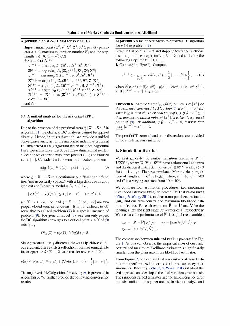
Figure 1. Comparison between rank and mle with accuracy measures (ηF , ηU , ηV ) versus number of state jumps n = C2rp log(p).

general problem (6) becomes the original rank-constraintmaximum likelihood problem (2).

Given X ∈ <p×p, let σ1(X) ≥ · · · ≥ σp(X) ≥ 0 bethe singular values of X. Since rank(X) ≤ r if and onlyσr+1(X) + . . . + σp(X) = ‖X‖∗ − ‖X‖(r) = 0, where‖X‖(r) =

∑ri=1 σi(X) is the Ky Fan r-norm of X, (6) can

be equivalently formulated as

minf(X) | ‖X‖∗ − ‖X‖(r) = 0, A(X) = b

.

See also (Gao & Sun, 2010, equation (29)). The penalizedformulation of problem (6) is

minX∈<p×p

f(X) + c(‖X‖∗ − ‖X‖(r)) | A(X) = b

, (7)

where c > 0 is a penalty parameter. Since ‖ · ‖(r) is convex,it is clear that the objective in problem (7) is a differenceof two convex functions: f(X) + c‖X‖∗ and c‖X‖(r), i.e.,(7) is a DC program.

Let X∗c be an optimal solution to the penalized problem(7). The following proposition shows that X∗c is also theoptimizer to (6) when it is low-rank.Proposition 2. If rank(X∗c) ≤ r, then X∗c is also an opti-mal solution to the original problem (6).

In practice, one can gradually increase the penalty param-eter c to obtain a sufficient low rank solution X∗c . In ournumerical experiments, we can obtain solutions with thedesired rank with a properly chosen parameter c.

5.2. A PDC algorithm for penalized problem (7)

The central idea of the DC algorithm (Pham Dinh & Le Thi,1997) is as follows: at each iteration, one approximates theconcave part of the objective function by its affine majorant,then solves the resulting convex optimization problem. Inthis subsection, we present a variant of the classic DC al-gorithm for solving (7). For the execution of the algorithm,we recall that the sub-gradient of Ky Fan r-norm at a pointX ∈ <p×p (Watson, 1993) is

∂‖X‖(r) =U Diag(q∗)VT | q∗ ∈ ∆

,

where U and V are the singular vectors of X, ∆ is theoptimal solution set of the following problem

maxq∈<p

p∑

i=1

σi(X)qi | 〈1p, q〉 = r, 0 ≤ q ≤ 1

.

Note that one can efficiently obtain a component of ∂‖X‖(r)by computing the SVD and picking up the SVD vectorscorresponding to the r largest singular values. After thesepreparations, we are ready to state the PDC algorithm forproblem (7). Different from the classic DC algorithm, anadditional proximal term is added to ensure the existenceof solutions of subproblems (8) and the convergence of thedifference of two consecutive iterations generated by thealgorithm. See Theorem 4 and Remark 6 for more details.

Algorithm 1 A PDC algorithm for solving problem (7)Given c > 0, α ≥ 0, and the stopping tolerance η, chooseinitial point X0 ∈ <p×p. Iterate the following steps fork = 0, 1, . . . :1. Choose Wk ∈ ∂‖Xk‖(r). Compute

Xk+1 = arg min

f(X) + c(‖X‖∗ − 〈Wk, X−Xk〉− ‖Xk‖(r)) +

α

2‖X−Xk‖2F

| A(X) = b

.

(8)2. If ‖Xk+1 −Xk‖F ≤ η, stop.

We say that X is a critical point of problem (7) if

∂(f(X) + c‖X‖∗) ∩ (c∂‖X‖(r)) 6= ∅.

We state the following convergence results for Algorithm 1.

Theorem 4. Let Xk be the sequence generated by Algo-rithm 1 and α ≥ 0. Then f(Xk) + c(‖Xk‖∗−‖Xk‖(r))is a non-increasing sequence. If Xk+1 = Xk for someinteger k ≥ 0, then Xk is a critical point of (7). Otherwise,


10 20 30 40 50 60 70 80 90 100

C

0.02

0.025

0.03

0.035

0.04

0.045

0.05

0.055

ηF

rank

svd

10 20 30 40 50 60 70 80 90 100

C

1.9

2

2.1

2.2

2.3

2.4

ηU

rank

svd

10 20 30 40 50 60 70 80 90 100

C

0

0.2

0.4

0.6

0.8

ηV

rank

svd

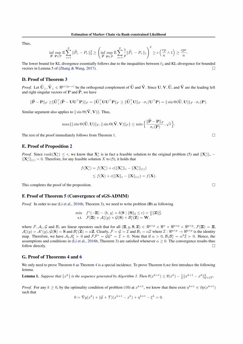
Figure 2. Comparison between rank and svd with accuracy measures (ηF , ηU , ηV ) VS. number of state jumps n = C2rp log(p).

it holds that(f(Xk+1) + c(‖Xk+1‖∗ − ‖Xk+1‖(r))

)

−(f(Xk) + c(‖Xk‖∗ − ‖Xk‖(r))

)

≤ − α

2‖Xk+1 −Xk‖2F .

Moreover, any accumulation point of the bounded sequenceXk is a critical point of problem (7). In addition, if α > 0,it holds that limk→∞ ‖Xk+1 −Xk‖F = 0.

Remark 6 (Selection of Parameters). In practice, a smallα > 0 is suggested to ensure strict decrease of the objectivevalue and convergence of ‖Xk+1−Xk‖F ; if f is stronglyconvex, one achieves these nice properties even if α = 0based on the results of Theorem 6. The penalty parameterc can be adaptively adjusted according to the rank of thesequence generated by Algorithm 1.

5.3. A multi-block ADMM for subproblem (8)

It is important and non-trivial to solve the convex subprob-lem (8) in Algorithm 1. Note that (8) is a nuclear normpenalized convex optimization problem, we propose to ap-ply an efficient multi-block alternating direction method ofmultipliers (ADMM) for solving the dual of (8). A compre-hensive numerical study has been conducted in (Li et al.,2016b) and justifies our procedure.

Instead of working directly on (8), we study a slightly gen-eral model as follows. Given W ∈ <p×p and α ≥ 0,consider

(P) min f(X) + 〈W, X〉+ c‖X‖∗ + α2 ‖X‖2F

s.t. A(X) = b.

Its dual problem can be written as

(D) min f∗(−Ξ)− 〈b, y〉+ α2 ‖Z‖2F

s.t. Ξ +A∗(y) + S + αZ = W, ‖S‖2 ≤ c,

where f∗ is the conjugate function of f , ‖ · ‖2 denotes thespectral norm. When we set f to be the negative likelihood

function (1), f∗ becomes

f∗(Ξ) =∑

(i,j)∈Ω

nijn

(lognijn− 1− log(−Ξij))

+∑

(i,j)∈Ω

δ(Ξij | Ξij ≤ 0) ∀Ξ ∈ <p×p,

where Ω = (i, j) | nij 6= 0 and Ω = (i, j) | nij =0. Given σ > 0, the augmented Lagrangian function Lσassociated with (D) is

Lσ(Ξ, y,S,Z; X) = f∗(−Ξ)− 〈b, y〉+α

2‖Z‖2F

+σ

2‖Ξ +A∗(y) + S + αZ−W + X/σ‖2 − 1

2σ‖X‖2.

We consider ADMM type methods for solving problem (D).Since there are four separable blocks in (D) (namely Ξ, y, S,and Z), the direct extended ADMM is not applicable. Fortu-nately, the functions corresponding to blocks y and Z in theobjective of (D) are linear-quadratic. Thus we can apply themulti-block symmetric Gauss-Sediel based ADMM (sGS-ADMM) (Li et al., 2016b). In literature (Chen et al., 2017;Ferreira et al., 2017; Lam et al., 2018; Li et al., 2016b; Wang& Zou, 2018), extensive numerical experiments demonstratethat sGS-ADMM is not only convergent but also faster thanthe directly extended multi-block ADMM and its manyother variants. Specifically, the algorithmic framework ofsGS-ADMM for solving (D) is presented in Algorithm 2.Note that when α = 0, the computation steps correspondingto block Z will not be performed.

When implementing Algorithm 2, only partial SVD, whichis much cheaper than full SVD, is needed as r p. Thefollowing convergence results can be directly obtained from(Li et al., 2016b). A sketch of the proof is given in supple-mentary material.Theorem 5. Suppose that the solution sets of (P) and (D)are nonempty. Let (Ξk, yk,Sk,Zk,Xk) be the sequencegenerated by Algorithm 2. If τ ∈ (0, (1 +

√5 )/2), then

the sequence (Ξk, yk,Sk,Zk) converges to an optimalsolution of (D) and Xk converges to an optimal solutionof (P).


Algorithm 2 An sGS-ADMM for solving (D)

Input: initial point (Ξ0, y0,S0,Z0,X0), penalty param-eter σ > 0, maximum iteration number K, and the step-length γ ∈ (0, (1 +

√5)/2)

for k = 0 to K doyk+ 1

2 = arg miny Lσ(Ξk, y,Sk,Zk; Xk)

Ξk+1 = arg minΞ Lσ(Ξ, yk+ 12 ,Sk,Zk; Xk)

yk+1 = arg miny Lσ(Ξk+1, y,Sk,Zk; Xk)

Zk+ 12 = arg minZ Lσ(Ξk+1, yk+1,Sk,Z; Xk)

Sk+1 = arg minS Lσ(Ξk+1, yk+1,S,Zk+ 12 ; Xk)

Zk+1 = arg minZ Lσ(Ξk+1, yk+1,Sk+1,Z; Xk)Xk+1 = Xk + γσ(Ξk+1 + A∗(yk+1) + Sk+1 +αZk+1 −W)

end for

5.4. A unified analysis for the majorized iPDCalgorithm

Due to the presence of the proximal term α2 ‖X−Xk‖2 in

Algorithm 1, the classical DC analyses cannot be applieddirectly. Hence, in this subsection, we provide a unifiedconvergence analysis for the majorized indefinite-proximalDC (majorized iPDC) algorithm which includes Algorithm1 as a special instance. Let X be a finite-dimensional real Eu-clidean space endowed with inner product 〈·, ·〉 and inducednorm ‖ · ‖. Consider the following optimization problem

minx∈X

θ(x) , g(x) + p(x)− q(x), (9)

where g : X → < is a continuously differentiable func-tion (not necessarily convex) with a Lipschitz continuousgradient and Lipschitz modulus Lg > 0, i.e.,

‖∇f(x)−∇f(x′)‖ ≤ Lg‖x− x′‖ ∀x, x′ ∈ X,

p : X → (−∞,+∞] and q : X → (−∞,+∞] are twoproper closed convex functions. It is not difficult to ob-serve that penalized problem (7) is a special instance ofproblem (9). For general model (9), one can only expectthe DC algorithm converges to a critical point x ∈ X of (9)satisfying

(∇g(x) + ∂p(x)) ∩ ∂q(x) 6= ∅.

Since g is continuously differentiable with Lipschitz continu-ous gradient, there exists a self-adjoint positive semidefinitelinear operator G : X→ X such that for any x, x′ ∈ X,

g(x) ≤ g(x;x′) , g(x′)+〈∇g(x′), x−x′〉+ 1

2‖x−x′‖2G .

The majorized iPDC algorithm for solving (9) is presented inAlgorithm 3. We further provide the following convergenceresults.

Algorithm 3 A majorized indefinite-proximal DC algorithmfor solving problem (9)Given initial point x0 ∈ X and stopping tolerance η, choosea self-adjoint linear operator T : X→ X and G. Iterate thefollowing steps for k = 0, 1, . . . :1. Choose ξk ∈ ∂q(xk). Compute

xk+1 ∈ arg minx∈X

θ(x;xk) +

1

2‖x− xk‖2T

, (10)

where θ(x;xk) , g(x;xk)+p(x)−(q(xk)+〈x−xk, ξk〉

).

2. If ‖xk+1 − xk‖ ≤ η, stop.

Theorem 6. Assume that infx∈X θ(x) > −∞. Let xk bethe sequence generated by Algorithm 3. If xk+1 = xk forsome k ≥ 0, then xk is a critical point of (9). If G+2T 0,then any accumulation point of xk, if exists, is a criticalpoint of (9). In addition, if G + 2T 0, it holds thatlimi→∞

‖xk+1 − xk‖ = 0.

The proof of Theorem 6 and more discussions are providedin the supplementary material.

6. Simulation ResultsWe first generate the rank-r transition matrix as P =UΣVT , where U,V ∈ <p×r have orthonormal columnsand the diagonal matrix Σ = diag(σi) ∈ <r×r with σi > 0for i = 1, . . . , r. Then we simulate a Markov chain trajec-tory of length n = C2rp log(p). Here, r = 10, p = 500and C is a varying constant from 10 to 102.

We compare four estimation procedures, i.e., maximumlikelihood estimator (mle), truncated SVD estimator (svd)(Zhang & Wang, 2017), nuclear norm penalized estimator(nu), and our rank-constrained maximum likelihood esti-mator (rank). For each estimator P, let U and V be theleading r left and right singular vectors of P, respectively.We measure the performance of P through three quantities:

ηF = ‖P− P‖F /√p, ηU = ‖ sin Θ(U, U)‖F ,

ηV = ‖ sin Θ(V, V)‖F .

The comparison between mle and rank is presented in Fig-ure 1. As one can observe, the empirical error of our rank-constrained maximum likelihood estimator is significantlysmaller than the plain maximum likelihood estimator.

From Figure 2, one can see that our rank-constrained esti-mator outperforms svd in terms of all three accuracy mea-surements. Recently, (Zhang & Wang, 2017) studied thesvd approach and developed the total variation error bounds.The rank-constrained estimator and the KL-divergence errorbounds studied in this paper are and harder to analyze and


10 20 30 40 50 60 70 80 90 100

C

0.02

0.04

0.06

0.08

0.1

0.12

0.14

ηF

rank

nu

10 20 30 40 50 60 70 80 90 100

C

1.8

2

2.2

2.4

2.6

2.8

3

ηU rank

nu

10 20 30 40 50 60 70 80 90 100

C

0

0.5

1

1.5

2

2.5

3

ηV rank

nu

Figure 3. Comparison between rank and nu with accuracy measures (ηF , ηU , ηV ) VS. number of state jumps n = C2rp log(p).

more meaningful for discrete distribution estimation.

In the implementation of nuclear norm penalized estima-tor nu, the penalty parameter is chosen via 5-fold cross-validation. The comparison between rank and nu is plottedin Figure 3. Clearly, the estimation error of rank is muchsmaller than that of nu. In fact, as one can see from Algo-rithm 1, the nuclear norm penalized estimator is in fact asingle step in the procedure of our rank-constrained estima-tor, and rank gradually refines based on nu. Theoreticallyspeaking, one could expect that, similar to the matrix re-covery (Recht et al., 2010), the rank-constrained estimatorenjoys better statistical performances and needs weaker as-sumption over the nuclear norm penalized estimator. More-over, Theorems 1 and 2 indicate that the rank-constrainedmaximum likelihood estimator is statistically optimal forthe estimation of Markov Chains. However, such a result isnot clear for the nuclear norm approach.

7. ConclusionThis paper studies the recovery and state compression oflow-rank Markov chains from empirical trajectories via arank-constrained likelihood approach. We provide statisticalupper bounds for the `2 risk and Kullback-Leiber divergencebetween the estimator and the true probability transitionmatrix for the proposed estimator. Then, a novel DC pro-gramming algorithm is developed to solve the associatedrank-constrained optimization problem. The proposed al-gorithm non-trivially combines several recent optimizationtechniques, such as the penalty approach, the proximal DCalgorithm, and the multi-block sGS-ADMM. We furtherstudy a new class of majorized indefinite-proximal DC al-gorithms for solving general non-convex non-smooth DCprogramming problems and provide a unified convergenceanalysis. Experiments on simulated data illustrate the meritsof our approach.

ReferencesAnandkumar, Animashree, Ge, Rong, Hsu, Daniel, Kakade,

Sham M, and Telgarsky, Matus. Tensor decompositionsfor learning latent variable models. The Journal of Ma-chine Learning Research, 15(1):2773–2832, 2014.

Azizzadenesheli, Kamyar, Lazaric, Alessandro, and Anand-kumar, Animashree. Reinforcement learning in rich-observation mdps using spectral methods. arXiv preprintarXiv:1611.03907, 2016.

Bertsekas, Dimitri P. Dynamic Programming and OptimalControl, volume 1. Athena scientific Belmont, MA, 1995.

Bertsekas, Dimitri P and Tsitsiklis, John N. Neuro-dynamicprogramming: an overview. In Decision and Control,1995., Proceedings of the 34th IEEE Conference on, vol-ume 1, pp. 560–564. IEEE, 1995.

Buchholz, Peter. Exact and ordinary lumpability in finiteMarkov chains. Journal of applied probability, 31(01):59–75, 1994.

Buhlmann, Peter and Van De Geer, Sara. Statistics for High-Dimensional Data: Methods, Theory and Applications.Springer Science & Business Media, 2011.

Chen, Liang, Sun, Defeng, and Toh, Kim-Chuan. An effi-cient inexact symmetric Gauss–Seidel based majorizedADMM for high-dimensional convex composite conicprogramming. Mathematical Programming, 161(1-2):237–270, 2017.

Deng, Kun and Huang, Dayu. Model reduction of Markovchains via low-rank approximation. In American ControlConference (ACC), 2012, pp. 2651–2656. IEEE, 2012.

Deng, Kun, Mehta, Prashant G, and Meyn, Sean P. Opti-mal Kullback-Leibler aggregation via spectral theory ofMarkov chains. IEEE Transactions on Automatic Control,56(12):2793–2808, 2011.


E, Weinan, Li, Tiejun, and Vanden-Eijnden, Eric. Optimalpartition and effective dynamics of complex networks.Proceedings of the National Academy of Sciences, 105(23):7907–7912, 2008.

Ferreira, Jose FS Bravo, Khoo, Yuehaw, and Singer, Amit.Semidefinite programming approach for the quadraticassignment problem with a sparse graph. ComputationalOptimization and Applications, pp. 1–36, 2017.

Gao, Yan and Sun, Defeng. A majorized penalty approachfor calibrating rank constrained correlation matrix prob-lems. technical reprot, 2010.

Han, Yanjun, Jiao, Jiantao, and Weissman, Tsachy. Minimaxestimation of discrete distributions under `1 loss. IEEETransactions on Information Theory, 61(11):6343–6354,2015.

Hsu, Daniel, Kakade, Sham M, and Zhang, Tong. A spectralalgorithm for learning hidden Markov models. Journal ofComputer and System Sciences, 78(5):1460–1480, 2012.

Huang, Qingqing, Kakade, Sham M, Kong, Weihao, andValiant, Gregory. Recovering structured probability ma-trices. arXiv preprint arXiv:1602.06586, 2016.

Kamath, Sudeep, Orlitsky, Alon, Pichapati, Dheeraj, andSuresh, Ananda Theertha. On learning distributions fromtheir samples. In Conference on Learning Theory, pp.1066–1100, 2015.

Keshavan, Raghunandan H, Montanari, Andrea, and Oh,Sewoong. Matrix completion from a few entries. IEEETransactions on Information Theory, 56(6):2980–2998,2010.

Lam, Xin Yee, Marron, J. S., Sun, Defeng, and Toh, Kim-Chuan. Fast algorithms for large-scale generalized dis-tance weighted discrimination. Journal of Computa-tional and Graphical Statistics, 27(2):368–379, 2018.doi: 10.1080/10618600.2017.1366915.

Le Thi, Hoai An and Pham Dinh, Tao. DC program-ming and DCA: thirty years of developments. Mathe-matical Programming, pp. 1–64, 2018. doi: 10.1007/s10107-018-1235-y.

Le Thi, Hoai An, Pham Dinh, Tao, and Van Ngai, Huynh.Exact penalty and error bounds in DC programming. Jour-nal of Global Optimization, 52(3):509–535, 2012.

Le Thi, Hoai An, Le, Hoai Minh, Phan, Duy Nhat, and Tran,Bach. Stochastic DCA for the large-sum of non-convexfunctions problem and its application to group variableselection in classification. In International Conferenceon Machine Learning, pp. 3394–3403, 2017.

Ledoux, Michel and Talagrand, Michel. Probability inBanach Spaces: Isoperimetry and Processes. SpringerScience & Business Media, 2013.

Lehmann, Erich L and Casella, George. Theory of pointestimation. Springer Science & Business Media, 2006.

Levin, David A and Peres, Yuval. Markov chains and mixingtimes, volume 107. American Mathematical Soc., 2017.

Li, Chris Junchi, Wang, Mengdi, Liu, Han, and Zhang, Tong.Diffusion approximations for online principal componentestimation and global convergence. In Advances in NeuralInformation Processing Systems, pp. 645–655, 2017.

Li, Chris Junchi, Wang, Mengdi, Liu, Han, and Zhang,Tong. Near-optimal stochastic approximation for on-line principal component estimation. Mathematical Pro-gramming, 167(1):75–97, Jan 2018. doi: 10.1007/s10107-017-1182-z.

Li, Min, Sun, Defeng, and Toh, Kim-Chuan. A majorizedADMM with indefinite proximal terms for linearly con-strained convex composite optimization. SIAM Journalon Optimization, 26(2):922–950, 2016a.

Li, Xudong, Sun, Defeng, and Toh, Kim-Chuan. A Schurcomplement based semi-proximal ADMM for convexquadratic conic programming and extensions. Mathemat-ical Programming, 155(1-2):333–373, 2016b.

Malek, Alan, Abbasi-Yadkori, Yasin, and Bartlett, Peter.Linear programming for large-scale Markov decisionproblems. In International Conference on Machine Learn-ing, pp. 496–504, 2014.

Moore, Andrew W. Variable resolution dynamic program-ming: Efficiently learning action maps in multivariatereal-valued state-spaces. In Machine Learning Proceed-ings 1991, pp. 333–337. Elsevier, 1991.

Negahban, Sahand and Wainwright, Martin J. Restrictedstrong convexity and weighted matrix completion: Op-timal bounds with noise. Journal of Machine LearningResearch, 13(May):1665–1697, 2012.

Negahban, Sahand, Oh, Sewoong, and Shah, Devavrat.Rank centrality: Ranking from pairwise comparisons.Operations Research, 65(1):266–287, 2016.

Newman, Mark EJ. Spectral methods for community de-tection and graph partitioning. Physical Review E, 88(4):042822, 2013.

Pham Dinh, Tao and Le Thi, Ho ai. Convex analysis ap-proach to DC programming: Theory, algorithms and ap-plications. Acta Mathematica Vietnamica, 22(1):289–355,1997.


Pham Dinh, Tao and Le Thi, Ho ai. The DC (differenceof convex functions) programming and DCA revisitedwith DC models of real world nonconvex optimizationproblems. Annals of operations research, 133(1-4):23–46,2005.

Recht, Benjamin. A simpler approach to matrix completion.Journal of Machine Learning Research, 12(Dec):3413–3430, 2011.

Recht, Benjamin, Fazel, Maryam, and Parrilo, Pablo A.Guaranteed minimum-rank solutions of linear matrixequations via nuclear norm minimization. SIAM review,52(3):471–501, 2010.

Singh, Satinder P, Jaakkola, Tommi, and Jordan, Michael I.Reinforcement learning with soft state aggregation. InAdvances in neural information processing systems, pp.361–368, 1995.

Steinhaus, Ho. The problem of estimation. The Annals ofMathematical Statistics, 28(3):633–648, 1957.

Sutton, Richard S and Barto, Andrew G. ReinforcementLearning: An Introduction, volume 1. MIT press Cam-bridge, 1998.

Tropp, Joel A. The expected norm of a sum of independentrandom matrices: An elementary approach. In High Di-mensional Probability VII, pp. 173–202. Springer, 2016.

Van Dinh, Bui, Kim, Do Sang, and Jiao, Liguo. Conver-gence analysis of algorithms for DC programming. arXivpreprint arXiv:1508.03899, 2015.

Van Roy, Benjamin. Performance loss bounds for approxi-mate value iteration with state aggregation. Mathematicsof Operations Research, 31(2):234–244, 2006.

Wang, Boxiang and Zou, Hui. Another look at distance-weighted discrimination. Journal of the Royal StatisticalSociety: Series B (Statistical Methodology), 80(1):177–198, 2018.

Watson, GA. On matrix approximation problems with KyFank norms. Numerical Algorithms, 5(5):263–272, 1993.

Wen, Bo, Chen, Xiaojun, and Pong, Ting Kei. A proxi-mal difference-of-convex algorithm with extrapolation.Computational Optimization and Applications, pp. 1–28,2017.

Yang, Lin F, Braverman, Vladimir, Zhao, Tuo, and Wang,Mengdi. Dynamic partition of complex networks. arXivpreprint arXiv:1705.07881, 2017.

Zhang, Anru and Wang, Mengdi. Spectral state compressionof Markov processes. arXiv preprint arXiv:1802.02920,2017.


A. Proof of Proposition 1Proof. Given xk = i, xk+1 is with discrete distribution Pi·. Thus, the log-likelihood of xk+1|xk = log(Pxk,xk+1

) =〈log(P), exk

e>xk+1〉. Then the negative log-likelihood given x0, . . . , xn is

−n∑

k=1

log(Pxk,xk+1) = −

n∑

k=1

〈log(P), exke>xk+1

〉 = −p∑

i=1

p∑

j=1

nij log(Pij).

B. Proof of Theorem 1Proof. Recall DKL(P,Q) =

∑pi=1 µiDKL(Pi·, Qi·) =

∑pj=1 µiPij log(Pij/Qij). For convenience, we also denote,

D(P,Q) =1

n

n∑

k=1

〈log(P)− log(Q),Ek〉,

where Ek = eie>j if the k-th jump is from States i to j. Then (Ek)nk=1 be independent copies such that P (Ek = eie

>j ) =

µiPij , and

L(P) = − 1

n

p∑

i,j=1

nij log(Pij) = − 1

n

n∑

k=1

log〈X,Ek〉

By the property of the programming,

D(P, P) =1

n

n∑

k=1

〈log(P)− log(P),Ek〉 = L(P)− L(P) ≤ 0. (11)

Based on the assumption, rank(P) ∧ rank(P) ≤ r. For any Q with rank(Q) ≤ r, we must have rank(Q−P) ≤ 2r. Dueto the duality between operator and spectral norm,

‖Q−P‖∗ ≤√

2r‖Q−P‖F . (12)

Next, we denote η = Cη√

log p/n for some large constant Cη > 0, and introduce the following deterministic set in Rp×p,

C = Q : α/p ≤ Qij ≤ β/p, rank(Q) ≤ r,DKL(P,Q) ≥ η .

We particularly aim to show next that

P

∀Q ∈ C,

∣∣∣D(P,Q)−DKL(P,Q)∣∣∣ ≤ 1

2DKL(P,Q) +

Cpr log(p)

n

≥ 1− Cp−c. (13)

In order to prove (13), we first split C as the union of the sets,

Cl =Q ∈ C : 2l−1η ≤ DKL(P,Q) ≤ 2lη, rank(Q) ≤ r

, l = 1, 2, 3, . . . .

where η is to be determined later. Define

γl = supQ∈Cl

∣∣∣DKL(P,Q)− D(P,Q)∣∣∣

= supQ∈Cl

∣∣∣∣∣1

n

n∑

k=1

〈log(P)− log(Q),Ek〉 − E〈log(P)− log(Q),Ek〉∣∣∣∣∣ .

Since | log(Pij)− log(Qij)| ≤ log(β/α), we apply a empirical process version of Hoeffding’s inequality (Theorem 14.2 in(Buhlmann & Van De Geer, 2011)),

P(γl − E(γl) ≥ 2l−3 · η

)≤ exp

(− cn · 4l−3η2

(log(β/α))2

). (14)


for constant c > 0. We generate εknk=1 as i.i.d. Rademacher random variables. By a symmetrization argument in empiricalprocess,

Eγl =E

(supQ∈Cl

∣∣∣∣∣1

n

n∑

k=1

〈log P− log Q,Ek〉 − E1

n

n∑

k=1

〈log P− log Q,Ek〉∣∣∣∣∣

)

≤2E

(supQ∈Cl

∣∣∣∣∣1

n

n∑

k=1

εk〈log P− log Q,Ek〉∣∣∣∣∣

).

Let φk(t) = α/p · 〈log(P)− log(Q + t),Ek〉, then φk(0) = 0 and |φ′k(t)| ≤ 1 for all t if t+ Pij ≥ α/p. In other words,φk,i,j is a contraction map for t ≥ mini,j(Pij − α/p). By concentration principle (Theorem 4.12 in (Ledoux & Talagrand,2013)),

E(γl) ≤2p

αE

(supQ∈Cl

∣∣∣∣∣1

n

n∑

k=1

εkφk (〈Q−P,Ek〉)∣∣∣∣∣

)

≤4p

αE

(supQ∈Cl

∣∣∣∣∣1

n

n∑

k=1

εk〈Q−P,Ek〉∣∣∣∣∣

)

≤4p

αE

(supQ∈Cl

∥∥∥∥∥1

n

n∑

k=1

εkEk

∥∥∥∥∥ · ‖Q−P‖∗

)

≤4p

αE

∥∥∥∥∥1

n

n∑

k=1

εkEk

∥∥∥∥∥ · supQ∈Cl

‖Q−P‖∗

(15)

By rank(P) ∧ rank(Q) ≤ r and Lemma 5 in (Zhang & Wang, 2017),

supQ∈Cl

‖Q−P‖∗(12)≤ sup

Q∈Cl

√2r‖Q−P‖F

≤

√√√√r(β/p)2

(α/p)

p∑

i=1

D(Pi·, Qi·) ≤√rβ2

α2· 2lη.

(16)

Then we evaluate E‖ 1n

∑nk=1 εkEk‖. Note that ‖Ek‖ ≤ 1,

‖n∑

k=1

EE>k Ek‖ =n

∥∥∥∥∥∥

p∑

i=1

p∑

j=1

µiPij(eie>j )>(eie

>j )

∥∥∥∥∥∥= n

∥∥∥∥∥∥

p∑

j=1

(µ>P )jeje>j

∥∥∥∥∥∥

=n

∥∥∥∥∥∥

p∑

j=1

µjeje>j

∥∥∥∥∥∥≤ nµmax;

‖n∑

k=1

EEkE>k ‖ =n

∥∥∥∥∥∥

p∑

i=1

p∑

j=1

µiPij(eie>j )(eie

>j )>

∥∥∥∥∥∥=

∥∥∥∥∥∥

p∑

i=1

p∑

j=1

µiPijeie>i

∥∥∥∥∥∥

=

∥∥∥∥∥∥

p∑

j=1

µjeje>j

∥∥∥∥∥∥≤ nµmax.

By Theorem 1 in (Tropp, 2016),

E

∥∥∥∥∥1

n

n∑

k=1

εkEk

∥∥∥∥∥ ≤C√nµmax log p

n+C log p

n≤ C

√µmax log p

n≤√β log p

np. (17)


provided that n ≥ Cp log(p). Combining (14), (15), (16), and (17), we have

Eγl ≤ C√pr log p

n· 2lη ≤ C2 pr log p

2n+ 2l−3η,

P

(γl ≥ 2l−2η +

Cpr log p

n

)≤ exp

(−cn · 4lη2

).

Now,

P

(∃Q ∈ C,

∣∣∣D(P,Q)−DKL(P,Q)∣∣∣ > 1

2DKL(P,Q) +

Cpr log(p)

n

)

≤∞∑

l=0

P

(∃Q ∈ Cl,

∣∣∣D(P,Q)−DKL(P,Q)∣∣∣ > 1

2DKL(P,Q) +

Cpr log(p)

n

)

≤∞∑

l=0

P

(∃Q ∈ Cl, γl > 2l−2η +

Cpr log(p)

n

)

≤∞∑

l=0

exp(−c · Cη · 4l log p) ≤ exp(−c · Cηl log(p)) ≤ Cp−c

provided reasonably large Cη > 0. Thus, we have obtained (13).

Finally, it remains to bound the errors for ‖P−P‖F and DKL(P, P) given (13). In fact, provided that (13) holds,

• if P /∈ C, we have DKL(P, P) ≤ C√

log pn ;

• if P ∈ C, by (13),

DKL(P, P) ≤ D(P, P) +Cpr log p

n

(11)≤ Cpr log p

n.

To sum up, we must have

DKL(P, P) ≤ C√

log p

n+Cpr log p

n.

with probability at least 1− Cp−c. For Frobenius norm error, we shall note that

‖P−P‖2F ≤p∑

i=1

‖Pi· − Pi·‖22 ≤p∑

i=1

2β2

αpDKL(Pi·, Pi·)

≤p∑

i=1

2β2

α2µiDKL(Pi·, Pi·) =

β2

α2DKL(P, P).

Therefore, we have finished the proof for Theorem 1.

C. Proof of Theorem 2Proof. Based on the proof of Theorem 1 in (Zhang & Wang, 2017), one has

infP

supP∈P

1

p

p∑

i=1

E‖Pi· − Pi·‖1 ≥ c(√

rp

n∧ 1

),

where P = P ∈ P : 1/(2p) ≤ Pij ≤ 3/(2p) ⊆ P . By Cauchy Schwarz inequality,

p∑

i=1

‖Pi· − Pi·‖1 =

p∑

i,j=1

|Pij − Pij | ≤ p

√√√√p∑

i,j=1

(Pij − Pij)2,


Thus,

infP

supP∈P

Ep∑

i=1

‖Pi· − Pi·‖22 ≥(

infP

supP∈P

Ep∑

i=1

1

p‖Pi· − Pi·‖1

)2

≥ c(rpn∧ 1)≥ cpr

n.

The lower bound for KL divergence essentially follows due to the inequalities between `2 and KL-divergence for boundedvectors in Lemma 5 of (Zhang & Wang, 2017).

D. Proof of Theorem 3Proof. Let U⊥, V⊥ ∈ <p×(p−r) be the orthogonal complement of U and V. Since U,V, U, and V are the leading leftand right singular vectors of P and P, we have

‖P−P‖F ≥‖U>⊥(P−UU>P)‖F = ‖U>⊥UU>P‖F ≥ ‖U>⊥U‖F · σr(U>P) = ‖ sin Θ(U,U)‖F · σr(P).

Similar argument also applies to ‖ sin Θ(V,V)‖. Thus,

max‖ sin Θ(U,U)‖F , ‖ sin Θ(V,V)‖F ≤ min‖P−P‖F

σr(P),√r.

The rest of the proof immediately follows from Theorem 1.

E. Proof of Proposition 2Proof. Since rank(X∗c) ≤ r, we know that X∗c is in fact a feasible solution to the original problem (5) and ‖X∗c‖∗ −‖X∗c‖(r) = 0. Therefore, for any feasible solution X to (5), it holds that

f(X∗c) = f(X∗c) + c(‖X∗c‖∗ − ‖X∗c‖(r))

≤ f(X) + c(‖X‖∗ − ‖X‖(r)) = f(X).

This completes the proof of the proposition.

F. Proof of Theorem 5 (Convergence of sGS-ADMM)Proof. In order to use (Li et al., 2016b, Theorem 3), we need to write problem (D) as following

min f∗(−Ξ)− 〈b, y〉+ δ(S | ‖S‖2 ≤ c) + α2 ‖Z‖2F

s.t. F(Ξ) +A∗1(y) + G(S) + B∗1(Z) = W,

where F ,A1,G and B1 are linear operators such that for all (Ξ, y,S,Z) ∈ <p×p × <n × <p×p × <p×p, F(Ξ) = Ξ,A∗1(y) = A∗(y), G(S) = S and B∗1(Z) = αZ. Clearly, F = G = I and B1 = αI where I : <p×p → <p×p is the identitymap. Therefore, we have A1A∗1 0 and FF∗ = GG∗ = I 0. Note that if α > 0, B1B∗1 = α2I 0. Hence, theassumptions and conditions in (Li et al., 2016b, Theorem 3) are satisfied whenever α ≥ 0. The convergence results thusfollow directly.

G. Proof of Theorems 4 and 6We only need to prove Theorem 6 as Theorem 4 is a special incidence. To prove Theorem 6,we first introduce the followinglemma.

Lemma 1. Suppose that xk is the sequence generated by Algorithm 3. Then θ(xk+1) ≤ θ(xk)− 12‖xk+1 − xk‖2G+2T .

Proof. For any k ≥ 0, by the optimality condition of problem (10) at xk+1, we know that there exist ηk+1 ∈ ∂p(xk+1)such that

0 = ∇g(xk) + (G + T )(xk+1 − xk) + ηk+1 − ξk = 0.


Then for any k ≥ 0, we deduce

θ(xk+1)− θ(xk) ≤ θ(xk+1;xk)− θ(xk)

= p(xk+1)− p(xk) + 〈xk+1 − xk,∇g(xk)− ξk〉+ 1

2‖xk+1 − xk‖2G≤ 〈∇g(xk) + ηk+1 − ξk, xk+1 − xk〉+ 1

2‖xk+1 − xk‖2G= − 1

2‖xk+1 − xk‖2G+2T .

This completes the proof of this lemma.

Now we are ready to prove Theorem 6.

Proof. From the optimality condition at xk+1, we have that

0 ∈ ∇g(xk) + (G + T )(xk+1 − xk) + ∂p(xk+1)− ξk.

Since xk+1 = xk, this implies that0 ∈ ∇g(xk) + ∂p(xk)− ∂q(xk),

i.e., xk is a critical point. Observe that the sequence θ(xk) is non-increasing since

θ(xk+1) ≤ θ(xk+1;xk) ≤ θ(xk;xk) = θ(xk), k ≥ 0.

Suppose that there exists a subsequence xkj that converging to x, i.e., one of the accumulation points of xk. By Lemma1 and the assumption that G + 2T 0, we know that for all x ∈ X

θ(xkj+1 ;xkj+1) = θ(xkj+1)

≤θ(xkj+1) ≤ θ(xkj+1;xkj ) ≤ θ(x;xkj ).

By letting j →∞ in the above inequality, we obtain that

θ(x; x) ≤ θ(x; x).

By the optimality condition of θ(x; x), we have that there exists u ∈ ∂p(x) and v ∈ ∂q(x) such that

0 ∈ ∇g(x) + u− v

This implies that (∇g(x) + ∂p(x)) ∩ ∂q(x) 6= ∅. To establish the rest of this proposition, we obtain from Lemma 1 that

limt→+∞

1

2

t∑

i=0

‖xk+1 − xk‖2G+2T

≤ lim inft→+∞

(θ(x0)− θ(xk+1)

)≤ θ(x0) < +∞ ,

which implies limi→+∞ ‖xk+1 − xi‖G+2T = 0. The proof of this theorem is thus complete by the positive definiteness ofthe operator G + 2T .

H. Discussions on G and THere, we discuss the roles of G and T . The majorization technique used to handle the smooth function g and the presence ofG are used to make the subproblems (10) in Algorithm 3 more amenable to efficient computations. As can be observed inTheorem 6, the algorithm is convergent if G + 2T 0. This indicates that instead of adding the commonly used positivesemidefinte or positive definite proximal terms, we allow T to be indefinite for better practical performance. Indeed, thecomputational benefit of using indefinite proximal terms has been observed in (Gao & Sun, 2010; Li et al., 2016a). In fact,


the introduction of indefinite proximal terms in the DC algorithm is motivated by these numerical evidence. As far as weknow, Theorem 6 provides the first rigorous convergence proof of the introduction of the indefinite proximal terms in theDC algorithms. The presence of G and T also helps to guarantee the existence of solutions for the subproblems (10). SinceG + 2T 0 and G 0, we have that 2G + 2T 0, i.e., G + T 0 (the reverse direction holds when T 0). Hence,G + 2T 0 (G + 2T 0) implies that subproblems (10) are (strongly) convex problems. Meanwhile, the choices of G andT are very much problem dependent. The general principle is that G + T should be as small as possible while xk+1 is stillrelatively easy to compute.

Estimation of Markov Chain via Rank-constrained Likelihood

Documents

Transcript of Estimation of Markov Chain via Rank-constrained Likelihood