Learning from short multivariate time series - ULisboa · HMM Hidden Markov model LL Log-likelihood...

Learning from short multivariate time series

José Maria Pedro Serra Líbano Monteiro

Thesis to obtain the Master of Science Degree in

Electrical and Computer Engineering

Supervisors: Prof. Alexandra Sofia Martins de CarvalhoProf. Susana de Almeida Mendes Vinga Martins

Examination Committee

Chairperson: Prof. João Fernando Cardoso Silva SequeiraSupervisor: Prof. Alexandra Sofia Martins de Carvalho

Members of the Committee: Prof. Mário Alexandre Teles de FigueiredoProf. Maria Margarida Campos da Silveira

December 2014

Agradecimentos

I want to thank my supervisors, Alexandra Carvalho and Susana Vinga, for their guidance throughout

the last year. Their support, availability and helpful remarks were essential for the development and

conclusion of this thesis.

I would also like to thank Prof. Helena Canhao and Prof. Joao Eurico Fonseca for providing the

rheumatoid arthritis dataset from Reuma.pt.

I acknowledge FCT, Fundacao para a Ciencia e a Tecnologia, for funding part of this work through

the project InteleGen (PTDC/DTPFTO/1747/2012).

Finally, I want to thank my family and friends for their support.

iii

Resumo

Em varios contextos de interesse e possıvel observar series temporais multivariadas (STM), que per-

mitem estudar a evolucao conjunta de um grupo de variaveis. A identificacao de dependencias con-

dicionais em STM pode ser feita atraves da aprendizagem da estrutura de redes de Bayes dinamicas

(RBD), que constituem uma ferramenta para representar processos temporais de uma forma compacta.

Varios metodos de aprendizagem de RBD focam-se apenas nas dependencias inter-temporais, nao

considerando a conectividade intra-temporal.

Esta dissertacao propoe um algoritmo de aprendizagem da estrutura de RBD que obtem conjunta-

mente as dependencias intra-temporais e inter-temporais. O espaco de solucoes e restringido a uma

classe de redes designada por arvores aumentadas, o que permite obter uma complexidade temporal

polinomial no numero de variaveis. O algoritmo tem a capacidade de aprender processos Markovianos

de ordem arbitraria, podendo ser estacionarios ou nao estacionarios. E tambem disponibilizada uma

implementacao em codigo livre do metodo proposto.

Numa primeira fase, o algoritmo e avaliado em dados simulados, observando-se que consegue

recuperar a estrutura subjacente aos mesmos de forma competitiva face aos algoritmos existentes.

Apos validacao inicial, o algoritmo e utilizado para identificacao de redes de regulacao genetica de

Drosophila melanogaster, e tambem para aprendizagem de dados clınicos referentes a doentes com

artrite reumatoide, com o objectivo de prever a evolucao da doenca. De uma forma geral, o algoritmo

proposto obteve bons resultados e pode ser considerado como alternativa para a aprendizagem da

estrutura de RBD.

Palavras-chave: series temporais multivariadas, redes de Bayes dinamicas, variaveis dis-

cretas, aprendizagem de estrutura, algoritmo polinomial

v

Abstract

Multivariate time series (MTS) arise in many interesting contexts and provide an opportunity for studying

the joint evolution of a group of variables. The identification of conditional dependences in MTS can be

achieved by learning the structure of dynamic Bayesian networks (DBN), a machine learning framework

for modelling temporal processes in a compact form. Several methods for DBN learning are concerned

with identifying inter time-slice dependences, but disregard the intra-slice connectivity.

This thesis proposes a DBN structure learning algorithm that jointly finds the optimal inter and intra

time-slice connectivity in a transition network. The search space is constrained to a class of networks

called tree-augmented DBN, leading to polynomial time complexity in the number of variables. The

algorithm can learn from stationary and non-stationary Markov processes with a fixed maximum lag.

Additionally, a free software implementation of the proposed method is made available.

An assessment of the algorithm is first made on simulated MTS, showing that the proposed method

is competitive with state of the art algorithms in recovering the structure underlying the data. Further

experimental validation is made on real data, by identifying non-stationary gene regulatory networks of

Drosophila melanogaster, and by learning from clinical data describing patients with rheumatoid arthritis,

in order to forecast the evolution of the disease. Overall, the proposed algorithm achieved good results

and can be considered as an alternative method for learning the structure of DBN.

Keywords: multivariate time series, dynamic Bayesian networks, discrete variables, structure

learning, polynomial-time algorithm

vii

Contents

Agradecimentos . . . . . . . . . . . . . . . . . . . . . . . . . . . . . . . . . . . . . . . . . . . . iii

Resumo . . . . . . . . . . . . . . . . . . . . . . . . . . . . . . . . . . . . . . . . . . . . . . . . . v

Abstract . . . . . . . . . . . . . . . . . . . . . . . . . . . . . . . . . . . . . . . . . . . . . . . . . vii

List of Tables . . . . . . . . . . . . . . . . . . . . . . . . . . . . . . . . . . . . . . . . . . . . . . xi

List of Figures . . . . . . . . . . . . . . . . . . . . . . . . . . . . . . . . . . . . . . . . . . . . . xiii

List of Algorithms . . . . . . . . . . . . . . . . . . . . . . . . . . . . . . . . . . . . . . . . . . . . xv

Glossary . . . . . . . . . . . . . . . . . . . . . . . . . . . . . . . . . . . . . . . . . . . . . . . . xvii

1 Introduction 1

1.1 Motivation . . . . . . . . . . . . . . . . . . . . . . . . . . . . . . . . . . . . . . . . . . . . . 1

1.2 Problem formulation . . . . . . . . . . . . . . . . . . . . . . . . . . . . . . . . . . . . . . . 1

1.3 Main approaches . . . . . . . . . . . . . . . . . . . . . . . . . . . . . . . . . . . . . . . . . 2

1.4 Scope of the thesis . . . . . . . . . . . . . . . . . . . . . . . . . . . . . . . . . . . . . . . . 3

1.5 Document outline . . . . . . . . . . . . . . . . . . . . . . . . . . . . . . . . . . . . . . . . . 4

2 Bayesian networks 5

2.1 Definition and related concepts . . . . . . . . . . . . . . . . . . . . . . . . . . . . . . . . . 5

2.2 Learning Bayesian networks . . . . . . . . . . . . . . . . . . . . . . . . . . . . . . . . . . 8

2.2.1 Scoring functions . . . . . . . . . . . . . . . . . . . . . . . . . . . . . . . . . . . . . 8

2.2.2 Search algorithms . . . . . . . . . . . . . . . . . . . . . . . . . . . . . . . . . . . . 10

2.3 Inference in Bayesian networks . . . . . . . . . . . . . . . . . . . . . . . . . . . . . . . . . 12

3 Dynamic Bayesian networks 15

3.1 Definition and assumptions . . . . . . . . . . . . . . . . . . . . . . . . . . . . . . . . . . . 15

3.2 Learning and inference . . . . . . . . . . . . . . . . . . . . . . . . . . . . . . . . . . . . . 17

3.3 Related work . . . . . . . . . . . . . . . . . . . . . . . . . . . . . . . . . . . . . . . . . . . 18

3.3.1 Structure learning . . . . . . . . . . . . . . . . . . . . . . . . . . . . . . . . . . . . 18

3.3.2 Real-world applications . . . . . . . . . . . . . . . . . . . . . . . . . . . . . . . . . 20

3.3.3 Software implementations . . . . . . . . . . . . . . . . . . . . . . . . . . . . . . . . 20

4 Proposed method 23

4.1 Optimal tree-augmented DBN structure learning . . . . . . . . . . . . . . . . . . . . . . . 24

ix

4.2 Complexity analysis . . . . . . . . . . . . . . . . . . . . . . . . . . . . . . . . . . . . . . . 29

4.3 Implementation . . . . . . . . . . . . . . . . . . . . . . . . . . . . . . . . . . . . . . . . . . 29

5 Experimental results 31

5.1 Simulated data . . . . . . . . . . . . . . . . . . . . . . . . . . . . . . . . . . . . . . . . . . 31

5.2 Drosophila melanogaster data . . . . . . . . . . . . . . . . . . . . . . . . . . . . . . . . . 37

5.3 Rheumatoid arthritis data . . . . . . . . . . . . . . . . . . . . . . . . . . . . . . . . . . . . 40

6 Conclusions 47

6.1 Achievements . . . . . . . . . . . . . . . . . . . . . . . . . . . . . . . . . . . . . . . . . . . 47

6.2 Future work . . . . . . . . . . . . . . . . . . . . . . . . . . . . . . . . . . . . . . . . . . . . 47

Bibliography 49

A Maximum branching algorithm 55

x

List of Tables

5.1 Comparative structure recovery results on simulated data. . . . . . . . . . . . . . . . . . . 33

5.2 Comparative structure learning results on Drosophila data. . . . . . . . . . . . . . . . . . 38

5.3 Characterization of the attributes in the preprocessed rheumatoid arthritis dataset. . . . . 41

5.4 Classification results on rheumatoid arthritis data. . . . . . . . . . . . . . . . . . . . . . . 43

5.5 Regression results on rheumatoid arthritis data. . . . . . . . . . . . . . . . . . . . . . . . . 44

xi

List of Figures

2.1 A simple BN example regarding airline regulations. . . . . . . . . . . . . . . . . . . . . . . 6

2.2 The BN example with conditional probability tables. . . . . . . . . . . . . . . . . . . . . . . 6

3.1 A simple first-order DBN structure example. . . . . . . . . . . . . . . . . . . . . . . . . . . 16

3.2 The DBN example unrolled for the first three time-slices. . . . . . . . . . . . . . . . . . . . 17

5.1 Network settings considered in simulated data experiments. . . . . . . . . . . . . . . . . . 32

5.2 Average structure recovery precision vs. number of observations on simulated data. . . . 35

5.3 Example of structure recovery vs. number of observations on simulated data. . . . . . . . 36

5.4 Drosophila gene regulatory networks identified by tDBN. . . . . . . . . . . . . . . . . . . . 39

5.5 Regression precision vs. error threshold on rheumatoid arthritis data. . . . . . . . . . . . 44

xiii

List of Algorithms

2.1 Chow-Liu tree learning . . . . . . . . . . . . . . . . . . . . . . . . . . . . . . . . . . . . . . 11

2.2 Belief propagation tree inference . . . . . . . . . . . . . . . . . . . . . . . . . . . . . . . . . 13

4.1 Optimal non-stationary first-order Markov tree-augmented DBN structure learning . . . . . 25

4.2 Determining edge weights and optimal sets of parents (first-order Markov) . . . . . . . . . 26

4.3 Optimal stationary first-order Markov tree-augmented DBN structure learning . . . . . . . . 27

4.4 Determining edge weights and optimal sets of parents (higher-order Markov) . . . . . . . . 28

A.1 Maximum branching: overview . . . . . . . . . . . . . . . . . . . . . . . . . . . . . . . . . . 55

A.2 Maximum branching: initializations . . . . . . . . . . . . . . . . . . . . . . . . . . . . . . . . 55

A.3 Maximum branching: branch procedure . . . . . . . . . . . . . . . . . . . . . . . . . . . . . 56

A.4 Maximum branching: leaf procedure . . . . . . . . . . . . . . . . . . . . . . . . . . . . . . . 57

xv

Glossary

2TBN Two-slice Bayesian network

BDe Bayesian Dirichlet equivalence

BIC Bayesian information criterion

CSV Comma-separated values

DAG Directed acyclic graph

DAS Disease activity score

DBN Dynamic Bayesian network

DNA Deoxyribonucleic acid

EM Expectation-maximization

FN False negative

FP False positive

HMM Hidden Markov model

LL Log-likelihood

MCMC Markov chain Monte Carlo

MDL Minimum description length

MIT Mutual information tests

MLE Maximum likelihood estimation

MRF Markov random field

MTS Multivariate time series

PDAG Partial directed acyclic graph

PGM Probabilistic graphic model

RA Rheumatoid arthritis

RMSE Root-mean-square error

RNA Ribonucleic acid

SEM Structural expectation-maximization

TAN Tree augmented naive Bayes

TN True negative

TP True positive

xvii

Chapter 1

Introduction

1.1 Motivation

Longitudinal data, also known as multivariate time series (MTS) in the machine learning community, are

obtained by conducting repeated measurements on a set of individuals. They arise in several contexts,

such as biomedical and clinical studies, socio-economics and meteorology, and provide an opportunity

for studying changes over time. In MTS, each measurement or observation is a vector of variables,

whose joint evolution is subject of analysis.

This work is concerned with short multivariate time series, where the number of measurements

ranges from two to a few dozens. As such, methods employed in long MTS prediction, which implic-

itly extrapolate past patterns into the future, cannot be applied in forecasting from short MTS, as past

patterns are hard to extrapolate from short MTS.

This thesis reviews current algorithms for learning dynamic Bayesian networks, as well as alterna-

tive methods for longitudinal data analysis. A new method is proposed, implemented and assessed in

synthetic and real data.

1.2 Problem formulation

A multivariate time series can be modelled as a set of n-dimensional observations of a stochastic pro-

cess over T sequential instants of time. The set of observations is expressed as xi[t]i∈I,t∈T ,, where I

is the set of individuals being measured and T is the set of time indices. Thus, xi[t] = (xi1[t], . . . , xin[t]) ∈

Rn is a single observation of n features, made at time t and referring to the individual i.

Observations are assumed to result from independent samples of a sequence of underlying probabil-

ity distributions Pθ[t]t∈T . While these distributions may be time-variant, they are considered constant

across different individuals observed at the same time, such that xi[t] ∼ Pθ[t] for all i ∈ I. If the obser-

vations are also identically distributed over time, that is, θ[t] = θ for all t ∈ T , the process is said to have

a stationary or time-invariant distribution (henceforth simply referred to as a stationary process).

While process stationarity is an adequate simplifying assumption in some cases, it does not hold in

1

many interesting scenarios. Consequently this thesis is also concerned with the general, more challeng-

ing case of non-stationarity. The scope of short MTS, which comprise a small number of observations,

further strengthens this choice.

The problem of learning from multivariate time series consists in estimating the relations among the

variables of the observed process, as well as their joint evolution throughout time. The relations to learn

can be divided in two groups: the intra-temporal relations, expressing the dependences between the

variables at a particular time instant t, and the inter-temporal relations, specifying how the variables

observed at times 0, . . . , t affect the variables at t+ 1.

1.3 Main approaches

A broad class of methods for learning time series can be found in literature [Hamilton, 1994]. This

section focuses on probabilistic graphical models (PGM), which constitute an important tool for analysing

multivariate processes and have been further extended to model temporal interactions [Dahlhaus, 2000].

Probabilistic graphical models describe complex processes that involve uncertainty [Murphy, 2001b;

Koller et al., 2007]. They provide an efficient way of representing a probability distribution, through the

use of a graph for encoding independence properties among the variables. Besides being an intuitive

visual representation, the underlying graph works as backbone for the computations that are performed

in the learning and inference operations [Ghahramani, 1998].

PGM may be generative or discriminative. Generative models define a joint probability distribu-

tion over all variables, aiming at describing (or generating) the entire data. In contrast, discriminative

models only specify a conditional distribution over a set of target variables given a set of observed

variables. They are often used for the tasks of classification and regression, since these do not re-

quire the specification of a marginal distribution over the observations. For example, given a set ob-

served variables x, one wishes to predict a set of label variables Y. Discriminative models directly

express the conditional distribution P (Y | x), whereas generative models describe the full joint proba-

bility P (Y,x) = P (Y | x) P (x). While the latter is a more ambitious approach, it is superfluous for the

task of classification, requiring useless effort to determine the marginal probability P (x).

There are two classes of PGM that are usually considered, Bayesian networks and Markov random

fields. While both models efficiently represent a joint distribution, they have distinct underlying seman-

tics, thus differing in the set of independences they can encode and in the factorization of the distribution

they can induce [Koller et al., 2007].

Directed graphical models, commonly called Bayesian networks (BN), are able to describe processes

whose variables directly influence each other in a certain direction [Pearl, 1988]. Informally speaking,

arcs in a BN can be thought as denoting causation, although this meaning does not usually hold in

reality. Because of the assumptions of conditional independence asserted by the graph, a BN defines a

joint probability distribution in a modular, very compact form.

On the other hand, undirected graphical models, also known as Markov networks or Markov random

fields (MRF), are adequate to describe processes where the relations between variables do not have an

2

implicit directionality [Koller et al., 2007]. These models also define a factorized representation of a joint

distribution, but in a less intuitive way than the one provided by BN.

The above mentioned graphical models are frequently used to represent static multivariate pro-

cesses, but are generally not suited for exploiting temporal aspects of time series data. Nevertheless,

they are easily extended to deal with dynamic processes. Dynamic Bayesian networks (DBN) model the

relations among the variables along sequential time steps. Arcs in a DBN flow forward in time, consis-

tently with the informal causality notion. They are often defined according to the rather strong first-order

Markov and stationarity assumptions, such that a pair of networks (a prior BN and a transition two-slice

BN, usually abbreviated as 2TBN) can describe the whole stochastic process [Friedman et al., 1998].

A Markov chain can be considered as the simplest DBN, consisting of a probabilistic transition of a

single observed variable. More generally, state-space models assume the existence of an underlying

hidden state of the process that generates the observations and evolves in time. A hidden Markov model

(HMM) [Rabiner and Juang, 1986] is a state-space model, having a discrete unobserved (hidden) state

that directly affects a multidimensional observed variable. A Kalman filter model is also a state-space

model, considering continuous variables and assuming that the state and the observations are jointly

Gaussian [Roweis and Ghahramani, 1999]. Both of these models can be seen as particular forms of

DBN [Murphy, 2002].

Finally, a conditional random field is a discriminative model that can be viewed as a MRF where

the target variables are globally conditioned on the observed variables. It is the discriminative analogue

to the HMM and has been shown to have advantages over it in classification problems [Sutton and

McCallum, 2010].

1.4 Scope of the thesis

Several learning and inference algorithms for time series models have recently been cast in the frame-

work of DBN [Grzegorczyk et al., 2008; Lebre et al., 2010; van der Heijden et al., 2013]. This thesis

considers DBN to address the problem of learning short MTS. The choice of DBN was primarily made

because of the expressiveness of the model and the dependences it can represent. In particular, in-

duced dependences are usually very important as a significant amount of information might be retrieved

from a collider in a v-structure.

The main contributions of this thesis are:

1. A theoretical overview on Bayesian networks, covering the main topics of causality, inference

and learning. A detailed state of the art review on non-stationary methods for learning dynamic

Bayesian networks, including real-world applications and available software implementations.

2. A new polynomial-time algorithm for learning the optimal structure of a specific class of dynamic

Bayesian networks, obtaining both the intra-slice and inter-slice connectivity. The algorithm was

implemented and made freely available.

3

3. An assessment of the developed method on simulated and real data, including comparisons to

other methods and to results obtained in other publications.

Some of the above findings resulted in the following article awaiting review in an international journal:

Monteiro, J. L., Vinga, S. and Carvalho, A. M. (2014). Polynomial-time algorithm for learning optimal

tree-augmented dynamic Bayesian networks. (Submitted to Pattern Recognition Letters).

1.5 Document outline

Chapter 2 gives a theoretical background on Bayesian networks. First, Section 2.1 presents the BN

definition, provides an example and explores the concepts of conditional independence and causality.

Then, Section 2.2 introduces the problem of learning BN using the search and score approach, and

Section 2.3 presents the task of inferring unobserved variables in BN.

Chapter 3 introduces dynamic Bayesian networks as a an extension to BN for modelling temporal

processes. Section 3.1 starts by defining DBN according to different assumptions. Section 3.2 extends

the concepts of learning and inference to DBN. Finally, Section 3.3 presents a review on methods for non-

stationary DBN structure learning, the current applications and a comparison of the available software

implementations.

Chapter 4 describes the proposed method for DBN structure learning. First, Section 4.1 presents

the tDBN algorithm, a proof of its optimality and its variations to stationarity and higher-order Markov

processes. Section 4.2 proceeds to derive a complexity bound on the algorithm’s running time. At last,

Section 4.3 describes the software implementation of the method.

Chapter 5 presents the results of several experiments to assess the developed method. Section 5.1

considers simulated data and compares the results to those obtained by a state of the art DBN learning

implementation. Then, in Section 5.2, the algorithm is employed to identify non-stationary gene regu-

latory networks of Drosophila melanogaster, and the results are compared with other authors’ findings.

Finally, Section 5.3 uses the developed algorithm to learn from clinical data resulting from patients with

rheumatoid arthritis, and an attempt is made to forecast an indicator of disease activity.

Chapter 6 presents the conclusions and future work.

4

Chapter 2

Bayesian networks

2.1 Definition and related concepts

In what follows, it holds the assumption that all random variables are discrete and have a finite domain.

Let X = (X1, . . . , Xn) be a random vector composed by random variables Xi, each having a domain

Xi ⊂ R. The elements of Xi are denoted by xi1, . . . , xiri , where ri is the number of values Xi can take,

i.e., the size of Xi.

A Bayesian network is a graphical representation of a joint probability distribution over a set of random

variables [Pearl, 1988]. It is defined as a triple B = (X, G,θ), where

• X = (X1, . . . , Xn) is a random vector;

• G = (X, E) is a directed acyclic graph (DAG) whose nodes correspond to the elements of X and

edges E specify conditional dependences between the variables: each Xi is independent of its

non-descendants given its parents1 pa(Xi) in G;

• θ = θijk is a set of parameters, specifying the local probability distributions of the network via

θijk = PB(Xi = xik | pa(Xi) = wij), (2.1)

where i ∈ 1, . . . , n, j ∈ 1, . . . , qi and k ∈ 1, . . . , ri. The set of possible configurations of

pa(Xi), i.e., the set of different combinations of values that the parents of Xi can take, is denoted

by wi1, . . . , wiqi, where qi =∏

Xj∈pa(Xi)rj is the number of all possible configurations.

A Bayesian network B defines a joint probability distribution over X:

PB(X1, . . . , Xn) =

n∏i=1

PB(Xi | pa(Xi)). (2.2)

For convenience, some notation regarding a dataset D used for learning a BN follows. Let D =

x`N`=1, where x` = (x`1, . . . , x`n) is the `-th instance in D. Within the dataset, Nijk is the number

1In a directed graph, a node u is a parent of node v if there is an arc going from u to v.

5

Maintenance problems

Flight delay

Severe weather

Cash compensationOvernight accommodation

Figure 2.1: A simple BN example regarding airline regulations.

P (M = T) = 0.02

P (S = T) = 0.03

F P (O = T|F )

T 0.3

F 0.01

M S P (F = T|M,S)

T T 0.95

T F 0.2

F T 0.6

F F 0.01

M

F

CO

SF S P (C = T|F, S)T T 0.05

T F 0.7

F T 0.01

F F 0.02

Figure 2.2: The BN example with conditional probability tables.

of instances where the variable Xi takes its k-th value xik and the variables in pa(Xi) take their j-th

configuration wij . Additionally, Nij is the number of instances where the variables in pa(Xi) take their

j-th configuration wij , notwithstanding the value of Xi, that is,

Nij =

ri∑k=1

Nijk. (2.3)

The total number of instances in D, denoted by N , can be obtained as

N =

n∑i=1

qi∑j=1

Nij . (2.4)

Example Figure 2.1 shows an example of a BN, describing common rules on compensation and as-

sistance to air passengers in the event of long delays of flights. A flight may be delayed due to the aircraft

having maintenance problems or due to severe weather conditions, such as a hurricane or a blizzard. A

passenger may be entitled to a monetary compensation if the delay was not caused by an external event

to the airline company. Regardless of the cause, if the delay is long enough, the passenger has the right

to be offered assistance such as overnight accommodation. In this simple example, all the variables take

binary values. Figure 2.2 introduces the probabilities of each variable being true, given all the possible

configurations of its parents. As a result of the dependences encoded by the graph, the joint probability

6

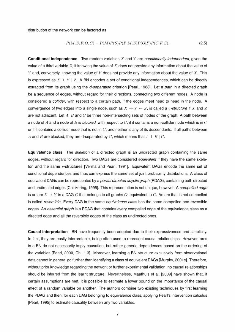
distribution of the network can be factored as

P (M,S, F,O,C) = P (M)P (S)P (F |M,S)P (O|F )P (C|F, S). (2.5)

Conditional independence Two random variables X and Y are conditionally independent, given the

value of a third variable Z, if knowing the value of X does not provide any information about the value of

Y and, conversely, knowing the value of Y does not provide any information about the value of X. This

is expressed as X ⊥⊥ Y | Z. A BN encodes a set of conditional independences, which can be directly

extracted from its graph using the d-separation criterion [Pearl, 1988]. Let a path in a directed graph

be a sequence of edges, without regard for their directions, connecting two different nodes. A node is

considered a collider, with respect to a certain path, if the edges meet head to head in the node. A

convergence of two edges into a single node, such as X → Y ← Z, is called a v-structure if X and Z

are not adjacent. Let A, B and C be three non-intersecting sets of nodes of the graph. A path between

a node of A and a node of B is blocked, with respect to C, if it contains a non-collider node which is in C

or if it contains a collider node that is not in C, and neither is any of its descendants. If all paths between

A and B are blocked, they are d-separated by C, which means that A ⊥⊥ B | C.

Equivalence class The skeleton of a directed graph is an undirected graph containing the same

edges, without regard for direction. Two DAGs are considered equivalent if they have the same skele-

ton and the same v-structures [Verma and Pearl, 1991]. Equivalent DAGs encode the same set of

conditional dependences and thus can express the same set of joint probability distributions. A class of

equivalent DAGs can be represented by a partial directed acyclic graph (PDAG), containing both directed

and undirected edges [Chickering, 1995]. This representation is not unique, however. A compelled edge

is an arc X → Y in a DAG G that belongs to all graphs G′ equivalent to G. An arc that is not compelled

is called reversible. Every DAG in the same equivalence class has the same compelled and reversible

edges. An essential graph is a PDAG that contains every compelled edge of the equivalence class as a

directed edge and all the reversible edges of the class as undirected ones.

Causal interpretation BN have frequently been adopted due to their expressiveness and simplicity.

In fact, they are easily interpretable, being often used to represent causal relationships. However, arcs

in a BN do not necessarily imply causation, but rather generic dependences based on the ordering of

the variables [Pearl, 2000, Ch. 1.3]. Moreover, learning a BN structure exclusively from observational

data cannot in general go further than identifying a class of equivalent DAGs [Murphy, 2001c]. Therefore,

without prior knowledge regarding the network or further experimental validation, no causal relationships

should be inferred from the learnt structure. Nevertheless, Maathuis et al. [2009] have shown that, if

certain assumptions are met, it is possible to estimate a lower bound on the importance of the causal

effect of a random variable on another. The authors combine two existing techniques by first learning

the PDAG and then, for each DAG belonging to equivalence class, applying Pearl’s intervention calculus

[Pearl, 1995] to estimate causality between any two variables.

7

2.2 Learning Bayesian networks

The problem of learning a Bayesian network B = (X, G,θ), given a dataset D comprising instances

of X, is stated as finding the structure G and the parameters θ such that B best matches D. One of

the approaches to this problem, that will be considered herein, consists in defining a scoring function

and a search procedure [Heckerman et al., 1995]. The scoring function φ(B,D) measures how well the

network B fits the dataset D, being related to the posterior probability of a network structure given the

data. The search procedure defines how to generate networks whose score is evaluated. Learning a

BN can be stated as the following optimization problem:

maximizeB∈Bn

φ(B,D), (2.6)

where Bn denotes the set of all BN with n variables.

Hardness results The number of possible structure hypotheses (DAGs) with n variables is more than

exponential in n. In fact, it has been shown that learning unrestricted BN from data, using a scoring

criterion, is NP-hard [Chickering et al., 1995]. Furthermore, limiting the number of parents of a node to

k is also NP-hard for k > 1 . Even restricting the search to polytrees2 with maximum in-degree of 2 is

NP-hard [Dasgupta, 1999]. Due to these results, polynomial-time algorithms for learning BN are limited

to finding tree structures. As a consequence, this work is mainly concerned with learning networks that

are represented by trees, because the number of variables can be quite large, even in the context of

short MTS.

2.2.1 Scoring functions

Many scoring criteria have been proposed in literature [Yang and Chang, 2002; Carvalho, 2009]. This

subsection presents two main properties regarding scoring functions, and provides the log-likelihood

and the minimum description length metrics as examples.

Score-equivalence An important property regarding scoring functions is score-equivalence. A scor-

ing function is score-equivalent if it evaluates the same value for equivalent networks. This is usually

a desired property, unless equivalent structures need to be distinguished, which happens when the di-

rectionality of the arcs has a special meaning, such as causality. Many of the commonly used scoring

criteria are score-equivalent, including the log-likelihood presented here.

Score-decomposability A scoring function is decomposable if it can be expressed as a sum of local

terms, each depending only on a node and its parents, that is,

φ(B,D) =

n∑i=1

φi(pa(Xi), D). (2.7)

2A polytree is a DAG whose skeleton is a tree. In contrast to a tree, nodes in a polytree can have more than one parent.

8

Decomposability simplifies the calculations of scores and provides an efficient way of evaluating incre-

mental changes on a network.

Log-likelihood A natural idea for a scoring function is to give a higher score to networks that are more

likely to have generated the data. This is accomplished by the likelihood function L(B : D) = P (D|B),

which measures the probability of data given the model. Since X is already known due toD and because

of the assumption of full observability (see Section 3.2), the model to be found is the pair (G,θG), where

θG is a set of parameters respecting the constraints imposed by G. According to the likelihood criterion,

the best model yields

maxG

L((G, θG) : D), (2.8)

where θG is obtained by maximizing the likelihood of the parameters θG given a fixed structure G. For a

multinomial distribution, the maximum likelihood estimation (MLE) for the parameters is given by

θG = θijk, (2.9)

where

θijk = PD(Xi = xik | pa(Xi) = wij) =Nijk

Nij(2.10)

and PD is the distribution induced by the observed frequency estimates. Equation (2.10) shows that

the parameters which give the most probable explanation for the data are simply obtained by counting

the different outcomes and calculating their frequencies. Since the parameters are trivially found for a

fixed network structure, given the data, the criterion depends only on the network G. Taking into account

Equation (2.2), and assuming that instances in D are i.i.d., the log-likelihood (LL) scoring criterion is

thus expressed [Heckerman et al., 1995] as

φLL(G,D) = logL(G : D)

=

N∑`=1

logPG(x`1, . . . , x

`n)

=

n∑i=1

qi∑j=1

ri∑k=1

Nijk log θijk

=

n∑i=1

qi∑j=1

ri∑k=1

Nijk logNijk

Nij.

(2.11)

The optimal structure is found by maximizing the previous expression over all possible structures G.

Generally, if the search space is not restricted, this criterion returns the complete graph, an effect com-

monly known as overfitting. The resulting model explains very well the training data, but fails to provide

good results on new cases. For this reason, the LL criterion is often extended to include a regularization

term, penalizing complex structures. Another possibility for avoiding overfitting is to limit the number

of parents each node is allowed to have, an approach that is considered in the Chow-Liu algorithm,

9

presented in Section 2.2.2.

Information-theoretic interpretation The derived expression for the LL scoring function can be inter-

preted from an information-theoretic point of view. To this objective, some background must be provided.

The mutual information of two random variables X and Y measures the mutual dependence between

them and is given by

I(X,Y ) =∑x,y

P (x, y) logP (x, y)

P (x)P (y). (2.12)

The entropy of a random variable X measures its expected uncertainty and is expressed as

H(X) = −∑x

P (x) logP (x). (2.13)

The LL criterion, given in Equation (2.11), can be reformulated as follows [Kollar and Friedman, 2009,

Ch. 18.3.1]:

φLL(G,D) =Nn∑

i=1

IPD(Xi,pa(Xi))−N

n∑i=1

HPD(Xi). (2.14)

As the second term of Equation (2.14) does not depend on the network structure, it can be disre-

garded when maximizing the expression over G. It becomes clear that LL gives an higher score to

networks which encode more informative relations among the nodes. The criterion effectively measures

the strength of the dependences between a node and its parents.

Other information-theoretic scores The minimum description length (MDL) score is an extension of

the LL criterion, including a term for penalizing complex structures:

φMDL(B,D) = φLL(G,D)− 1

2log(N)|B|, (2.15)

where |B| denotes the number of parameters of the network, given by

|B| =n∑

i=1

(ri − 1)qi. (2.16)

The MDL score coincides with the Bayesian information criterion (BIC) [Schwarz, 1978]. Another rele-

vant score is the more recent mutual information tests (MIT) [de Campos, 2006], which penalizes the

degree of interaction among the variables by a term related to Pearson’s χ2 test of independence.

2.2.2 Search algorithms

Due to the already stated hardness results, finding an optimal BN in polynomial time requires restricting

the search space to tree structures. An algorithm for solving this problem was developed by Chow and

Liu [1968] and is described in the following. A generic algorithm to find a locally optimal solution without

an a priori restriction on the search space is also presented.

10

Chow-Liu tree learning The Chow-Liu algorithm, originally presented before BN were formalized,

addresses the problem of approximating a joint probability distribution by a product of component dis-

tributions. It builds a tree with maximum mutual information, which is equivalent to building a tree with

maximum log-likelihood score, as seen in Section 2.2.1. For the purpose of being used as a BN struc-

ture, the resulting tree needs to be converted into a directed graph. This is done by arbitrarily choosing

a node as root and directing all edges outwards from it.

Algorithm 2.1: Chow-Liu tree learning

Input: X: a set of random variables;

D: a dataset comprising instances of X

Output: A tree graph, with X as nodes, maximizing the mutual information of the random variables

1 Build a complete undirected graph in X

2 For each Xi, Xj ∈ X, i 6= j :

3 Calculate the mutual information I(Xi, Xj) and assign this value as the weight of an

undirected edge between Xi and Xj

4 Apply a maximum weight spanning tree algorithm

The algorithm can be easily adapted to work with different metrics, including non score-equivalent

ones [Heckerman et al., 1995]. To deal with a different metric φ, the weight of an edge between Xi

and Xj is assigned as φj(Xi, D) − φj(, D), which is equal to φi(Xj, D) − φi(, D) when φ is

score-equivalent, and expresses the the contribution of the edge, as measured by φ, to the total network

score. If the used score is not score-equivalent, the weight of an edge may be direction dependant.

Consequently, the built complete graph is directed and the number of weights to compute duplicates. In

this case, a maximum weight directed spanning tree, also known as maximum branching, must be found

instead. The Edmonds’ algorithm [Edmonds, 1967] can be applied for this purpose.

Greedy hill climbing The hill climbing method belongs to the family of local search heuristics, which

are employed to solve hard optimization problems, such as the one of learning BN stated in Equation

(2.6). Hill climbing works by traversing the search space, starting from an initial solution and performing

a finite number of iterations. At each step, the algorithm considers local changes to the current structure,

such as the addition, deletion, or reversal of a single edge, and proceeds with the one which yields the

best gain in the scoring function [Gamez et al., 2011]. The use of a decomposable score allows an

efficient computation of the score metric at each iteration, due to the incremental changes in the graph.

When no further improvement can be made, the algorithm has reached a local optimum and stops. In

general, this greedy behaviour does not lead to a globally optimal solution, and the algorithm is said

to be trapped at a local solution. Some techniques, like restarting the search or introducing a random

component, are often employed to try to escape from local optima.

11

2.3 Inference in Bayesian networks

Since a graphical model provides a joint probability distribution, a useful task that can be performed is

estimating the value of unobserved variables Y ⊂ X, given a set of observed evidence e. This is the

main goal of inference, which relies on Bayes’ rule:

P (Y|e) = P (e|Y)P (Y)

P (e). (2.17)

In the above equation, P (Y|e) is often called the posterior, and expresses the resulting distribution

over Y conditioned on the possible knowledge provided by e. The uncertainty regarding Y, before

the evidence is observed, is expressed by the probability distribution P (Y), known as the prior. The

term P (e|Y) is called the likelihood and measures the compatibility of the evidence with the possible

configurations of Y.

Hardness results Performing inference using Bayes’ rule is generally intractable. It has been shown

that exact probabilistic inference on a generic BN is NP-hard [Cooper, 1990]. Moreover, even finding

an approximation for the values of unobserved nodes is an NP-hard problem, requiring an exponential

number of operations [Dagum and Luby, 1993]. While these hardness results are to some extent similar

to those obtained when considering the task of learning, there are in practice heuristic methods that

provide good estimates in reasonable time. For the special class of tree networks, the inference problem

can be solved efficiently in polynomial time complexity.

Belief propagation

The belief propagation algorithm for performing exact inference in a tree network was presented by

Pearl [1982]. Given a set of evidence variables E taking the values e, it allows the computation of the

conditional probabilities P (Yi|e) for all unobserved Yi nodes. To do so, all nodes send messages to

their neighbours and process the received messages, making use of their local probability distributions.

Before describing the algorithm, some concepts need to be defined [Neapolitan, 2004, Ch. 3.2.1].

Considering a node X, it divides the network into two disjoint parts (as it is a tree). Let E+ be the set

of evidence nodes which can be accessed via the (single) parent of X, denoted by pa(X). Conversely,

E− is the set of evidence nodes that can be reached through the children of X, denoted by ch(X). The

sets E+ and E− respectively take the sets of observed values e+ and e−. The conditional probability of

X taking a value x given the evidence, also called the belief in x, is given by

P (x|e) = P (x|e−, e+)

= αP (e−|x)P (x|e+)

= αλ(x)π(x),

(2.18)

where α is a normalization constant and, in general, λ(x) results from the messages sent by the children

of X and π(x) results from a message sent by the parent of X.

12

The values λ(x) are defined depending on the position of X in the network structure and whether it

belongs to the set of observed variables. Each case is addressed in the following. If X is an evidence

node and it takes the value x, it holds that λ(x) = 1 and λ(x) = 0 for all x 6= x. If X is not observed and

it is a leaf, i.e., X does not have any children, λ(x) = 1 for all x. The last case arises when X is neither

a leaf nor an evidence node, which yields

λ(x) =∏

Xc∈ch(X)

λXc→X(x), (2.19)

where each λXc→X(x) denotes a message sent from Xc to X and is given by

λXc→X(x) =∑

xi∈Xc

P (xi|x)λ(xi), (2.20)

recalling that Xc is the domain of Xc.

The values π(x) are defined according to similar conditions. If X is an evidence node and it takes

the value x, it holds that π(x) = 1 and π(x) = 0 for all x 6= x. If X is not observed and it is the root of the

tree, i.e., X does not have a parent, π(x) = P (x) for all x. When X is not the root nor is it observed,

π(x) =∑

xi∈Xpa(X)

P (x|xi)πpa(X)→X(xi), (2.21)

where πpa(X)→X(xi) denotes a message sent from pa(X) to X for each xi, given by

πpa(X)→X(xi) = π(xi)∏

Xc∈ch(pa(X))\X

λXc→pa(X)(xi). (2.22)

Algorithm 2.2: Belief propagation tree inference

Input: B = (X, G,θ): a Bayesian network

E← e: set of evidence variables and their observed values

Output: The resulting joint probability distribution P (Y|e), Y = X \E

1 Every leaf node Xl initializes λ(xl) for all xl ∈ Xl, which will be the messages for pa(Xl)

2 Every evidence node Xe ∈ E initializes its λ(xe) values

3 Starting from the leaves, messages are propagated upwards in the tree until they reach the root,

such that all nodes are able to compute their own λ values according to Equation (2.19)

4 The root node Xr initializes its values π(xr) for all xr ∈ Xr, which will be the messages for nodes

in ch(Xr)

5 Starting from the root, messages are propagated downwards in the tree until they reach the

leaves, such that all nodes are able to compute their own π values according to Equation (2.21)

6 All nodes can compute their belief values according to Equation (2.18)

13

Chapter 3

Dynamic Bayesian networks

While a BN defines a joint probability distribution over a fixed set of variables, a dynamic Bayesian

network extends this representation to model temporal processes [Friedman et al., 1998].

3.1 Definition and assumptions

Let X = (X1, . . . , Xn) be a random vector composed by the attributes that the are changed by some

process. The same assumptions as for BN, regarding the domain and notation of the variables, are con-

sidered. Let X[t] = (X1[t], . . . , Xn[t]) be a random vector that denotes the instantiation of the attributes

at time t. In addition, X[t1 : t2] denotes the set of random vectors X[t] for t1 ≤ t ≤ t2. For instance,

X[0 : T ] = X[0] ∪ · · · ∪X[T ], for T ≥ 0. Let P (X[0], . . . ,X[T ]), abbreviated by P (X[0 : T ]), denote the

joint probability distribution over the temporal trajectory of the process from X[0] to X[T ].

A dynamic Bayesian network is a representation of the joint probability distributions over all possible

trajectories of a process. It is composed by:

• a prior network B0, which specifies a distribution over the initial states X[0];

• a set of transition networks Bt0 over the variables X[0 : t], specifying the state transition probabili-

ties, for 0 < t ≤ T .

In the previous definition, the timeline is discretized into several time-slices, each comprising mea-

surements of the process at a specific time instant. Slices are equally spaced in time, which means

that the sampling interval is constant. As the temporal trajectories can be extremely complex, further

simplifying assumptions on the process are usually made.

A common premise is to consider first-order Markov processes, in which future values only depend

on present ones but not on the past trajectory, such that P (X[t + 1] | X[0 : t]) = P (X[t + 1] | X[t]). A

relaxation of this memoryless assumption is the higher-order Markov property, where nodes can have

dependences on an arbitrary (but fixed) number of previous time-slices. For instance, in a m-th-order

Markov process, P (X[t+1] | X[0 : t]) = P (X[t+1] | X[t−m+1 : t]), for some integer m > 0. m is also

called the (maximum) Markov lag of the process.

15

Turning signal [0]

Distance to next [0]

Speed [0]

Lane [0]

Turning signal [0]


Lane [1]

Speed [0]

Lane [0]


Turning signal [1]

Speed [1]

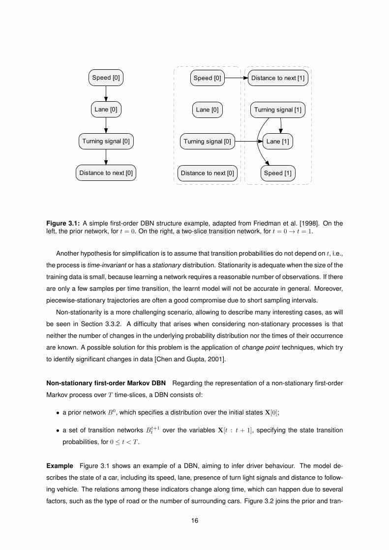
Figure 3.1: A simple first-order DBN structure example, adapted from Friedman et al. [1998]. On theleft, the prior network, for t = 0. On the right, a two-slice transition network, for t = 0→ t = 1.

Another hypothesis for simplification is to assume that transition probabilities do not depend on t, i.e.,

the process is time-invariant or has a stationary distribution. Stationarity is adequate when the size of the

training data is small, because learning a network requires a reasonable number of observations. If there

are only a few samples per time transition, the learnt model will not be accurate in general. Moreover,

piecewise-stationary trajectories are often a good compromise due to short sampling intervals.

Non-stationarity is a more challenging scenario, allowing to describe many interesting cases, as will

be seen in Section 3.3.2. A difficulty that arises when considering non-stationary processes is that

neither the number of changes in the underlying probability distribution nor the times of their occurrence

are known. A possible solution for this problem is the application of change point techniques, which try

to identify significant changes in data [Chen and Gupta, 2001].

Non-stationary first-order Markov DBN Regarding the representation of a non-stationary first-order

Markov process over T time-slices, a DBN consists of:

• a prior network B0, which specifies a distribution over the initial states X[0];

• a set of transition networks Bt+1t over the variables X[t : t + 1], specifying the state transition

probabilities, for 0 ≤ t < T .

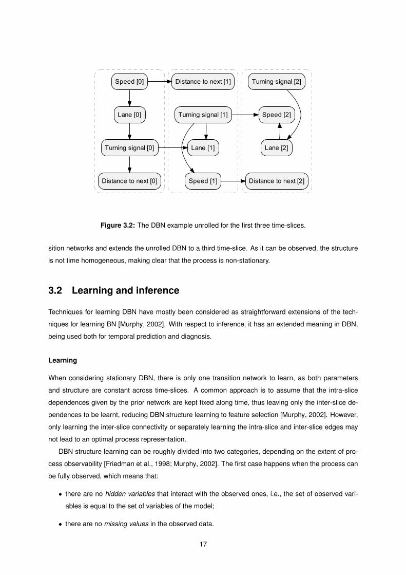
Example Figure 3.1 shows an example of a DBN, aiming to infer driver behaviour. The model de-

scribes the state of a car, including its speed, lane, presence of turn light signals and distance to follow-

ing vehicle. The relations among these indicators change along time, which can happen due to several

factors, such as the type of road or the number of surrounding cars. Figure 3.2 joins the prior and tran-

16

Turning signal [0]


Lane [1]

Speed [0]

Lane [0]


Turning signal [1]

Speed [1]

Speed [2]


Turning signal [2]

Lane [2]

Figure 3.2: The DBN example unrolled for the first three time-slices.

sition networks and extends the unrolled DBN to a third time-slice. As it can be observed, the structure

is not time homogeneous, making clear that the process is non-stationary.

3.2 Learning and inference

Techniques for learning DBN have mostly been considered as straightforward extensions of the tech-

niques for learning BN [Murphy, 2002]. With respect to inference, it has an extended meaning in DBN,

being used both for temporal prediction and diagnosis.

Learning

When considering stationary DBN, there is only one transition network to learn, as both parameters

and structure are constant across time-slices. A common approach is to assume that the intra-slice

dependences given by the prior network are kept fixed along time, thus leaving only the inter-slice de-

pendences to be learnt, reducing DBN structure learning to feature selection [Murphy, 2002]. However,

only learning the inter-slice connectivity or separately learning the intra-slice and inter-slice edges may

not lead to an optimal process representation.

DBN structure learning can be roughly divided into two categories, depending on the extent of pro-

cess observability [Friedman et al., 1998; Murphy, 2002]. The first case happens when the process can

be fully observed, which means that:

• there are no hidden variables that interact with the observed ones, i.e., the set of observed vari-

ables is equal to the set of variables of the model;

• there are no missing values in the observed data.

17

A fully observed process can be learnt using the previously discussed search and score approach (see

Section 2.2), which tries to find the best network over the space of models.

The second category concerns partially observed processes, where there are hidden variables

and/or missing data. Several difficulties arise in this case, mainly that partial observations are not

Markov even if the process has this property, and scoring functions no longer decompose. Friedman

[1997] proposed the structural expectation-maximization (SEM) iterative method to solve these prob-

lems. SEM alternates between evaluating the expected score of a model, using an inference engine,

and changing the model structure, until a local maximum is reached [Murphy and Mian, 1999].

Regarding the hardness results, it was recently shown that learning the structure of a DBN, unlike

the case for a static BN, does not necessarily have to be NP-hard [Dojer, 2006] . This is due to the

relaxation of the acyclicity constraint on the inter-sliced transition network, since the unrolled network is

always acyclic. A polynomial complexity bound in the number of variables was derived for the Bayesian

Dirichlet equivalence (BDe) and MDL scores in the same article. Relying on Dojer [2006], Vinh et al.

[2011b] further proposed an optimal polynomial-time algorithm for learning DBN using the information-

theoretic MIT score.

Inference Similarly to what respects BN, inference refers to estimating the value of unobserved vari-

ables given a set of observed ones, called the evidence nodes. However, in the context of DBN, this

operation has a broader meaning, as it can refer to inferring values at arbitrary time-slices. When the

evidence is given for a time t0 and the goal is to estimate values for a past time t < t0, this is known as

smoothing. When inference is done for the present time t = t0, the operation is called filtering. If one

wishes to estimate values on a future time t > t0, this is known as prediction. Although these operations

have different semantics, the techniques used to perform them are the same [Murphy, 2002].

3.3 Related work

3.3.1 Structure learning

While there is plenty of literature regarding the process of learning stationary first-order Markov net-

works, there are only a few references to learning more general classes of DBN. In fact, it was not until

recently that some authors started to relax the standard stationarity assumption underlying graphical

models. The next paragraphs review the state of the art of such realizations.

The problem of model selection, that is, identifying a system for probabilistic inference that is efficient,

accurate and informative is discussed by Bilmes [2000]. With the purpose of performing classification,

the author proposes a class of models called dynamic Bayesian multinets, where the conditional inde-

pendences are determined by the values of certain nodes in the graph, instead of being fixed. This is

accomplished by extending HMM to include dependences among observations of different time steps.

The idea of a network whose edges can appear and disappear is further explored by other authors in a

temporal context to model non-stationary processes.

18

Tucker and Liu [2003] follow the same line of work as Bilmes [2000], incorporating hidden nodes in

the DBN model. These nodes determine how the variables behave based upon their current state, thus

acting as controllers of time-varying dependences. A hill climbing procedure is employed to learn the

network structure. Referring to this work, Flesch and Lucas [2007] acknowledge that stationarity is a

strong assumption that usually does not hold and propose a new DBN framework where temporal and

non-temporal independence relations are separated.

Robinson and Hartemink [2009] define an extension of the traditional DBN model, and take the ap-

proach of learning an initial network of dependences and a set of incremental changes on its structure.

The authors assume that the process is piecewise-stationary, having the number and times of the tran-

sitions (change points) to be estimated a posteriori. Prior knowledge regarding both the initial structure

and the evolutionary behaviour of the network can be incorporated. By considering conjugate Dirichlet

priors on the parameters, which are assumed to have a multinomial distribution, the marginal likelihood

is computed exactly, resulting in the BDe metric. The authors extend this metric to incorporate the

changes introduced by their new model. For conducting the search procedure, they use a sampling

strategy based on the Markov chain Monte Carlo (MCMC) method, allowing faster convergence than

expectation-maximization (EM) techniques.

Dondelinger et al. [2010] follow the same approach, but consider continuous data. The authors

differentiate the penalties for adding and deleting edges in the network, as removing a critical regulatory

edge is a more relevant change than including a redundant connection. Moreover, they allow different

nodes of the network to have distinct penalty terms, instead of a single hyperparameter for penalizing

disparities between structures. Another differing aspect is that Robinson and Hartemink [2009] consider

change points regarding the whole network while Dondelinger et al. [2010] allow node-specific change

points, leading to a more flexible model.

Grzegorczyk and Husmeier [2009] propose a non-stationary model that comprises a fixed network

structure with time-varying parameters. The common structure is intended to provide information shar-

ing across time-slices, while the parameters account for changes in the process. The same node change

points technique as in Dondelinger et al. [2010] is employed. The authors advocate the fixed network

structure as a solution to model over-flexibility, a problem that almost inevitably results from modelling

short time series with several networks. On the other hand, Husmeier et al. [2010] note that this as-

sumption is too rigid to represent processes where changes in the overall regulatory network structure

are expected.

In more recent work, Grzegorczyk and Husmeier [2012] argue that there should be a trade-off be-

tween the often unrealistic stationarity assumption, modelled with constant parameters, and the opposite

case of complete parameter independence over time, ignoring the evolutionary aspect of the process.

They acknowledge, however, that the latter case, which is considered by Robinson and Hartemink [2009]

and Dondelinger et al. [2010], has the advantage of allowing the computation of the marginal likelihood

in closed form. The authors, also working in the continuous domain, introduce a scheme for coupling

the parameters along time-slices, although keeping the network structure fixed, as considered in Grze-

gorczyk and Husmeier [2009].

19

Regarding undirected graphical models, Kolar et al. [2010] propose two methods for estimating the

underlying time-varying networks of a stochastic process. They model each network as a MRF with

binary nodes. The first method assumes that the parameters change smoothly over time whereas the

second considers piecewise constant parameters with abrupt changes. In both approaches, the esti-

mator for the parameters is the result of a l1-regularized convex optimization problem. These methods,

however, only capture pairwise undirected relations between binary variables, resulting in a model that

is far from general application.

3.3.2 Real-world applications

A very frequent application of DBN structure learning is the identification of genetic regulatory systems

[Murphy and Mian, 1999; Husmeier, 2003; Zou and Conzen, 2005]. These networks model the reg-

ulatory interactions between DNA, RNA, proteins and small molecules [De Jong, 2002], and explicitly

represent the causality of developmental processes [Davidson and Levin, 2005]. Murphy and Mian

[1999] note that models learnt from data should be subject to experimental verification, which is usually

feasible in molecular biology.

Recent efforts have been made to model time-varying gene interactions [Grzegorczyk et al., 2008;

Lebre et al., 2010]. A frequently studied organism is the Drosophila melanogaster (common fruit fly),

whose gene expression patterns during a complete life cycle were made available [Arbeitman et al.,

2002]. Several authors use this dataset to learn time-varying dependences [Zhao et al., 2006; Guo

et al., 2007; Robinson and Hartemink, 2009; Dondelinger et al., 2010] and/or to assess correct change

points identification [Robinson and Hartemink, 2009; Lebre et al., 2010]. Another common example is

the Saccharomyces cerevisiae (yeast) [Husmeier et al., 2010; Grzegorczyk and Husmeier, 2012].

DBN are also used to model clinical data, describing the progression of a disease over time for

prediction purposes [van Gerven et al., 2008; Charitos et al., 2009; van der Heijden et al., 2013]. For

instance, van der Heijden et al. [2013] study the evolution of chronic obstructive pulmonary disease to

detect and possibly prevent episodes of decreased health status. They note that analysing clinical time

series is a challenging task because of insufficient data, irregular time intervals and missing values.

These problems arise due to the low frequency of the event of interest, the cost of taking measurements

and the inconvenience caused to patients.

3.3.3 Software implementations

Although there are many software implementations for BN inference and learning [Murphy, 2007], only

a minority is both freely available and able to deal with DBN structure learning. Some of the implemen-

tations that fall under both categories are briefly described in the following. It is important to note that

none of them supports non-stationary networks.

BNT: Bayes Net Toolbox for Matlab [Murphy, 2001a] is a very popular tool that comprises a wide

range of inference and learning algorithms. However, it only provides one structure learning algorithm

for DBN, which assumes full process observability and no intra-slice connectivity. BNT is well known for

20

its extensively documented source code.

Banjo: Bayesian Network Inference with Java Objects [Hartemink et al., 2005] focuses on score-

based structure learning, applying local search heuristics using the BDe metric. Available heuristic

search strategies include simulated annealing and greedy hill-climbing, paired with evaluation of a single

random local move or all local moves at each step. A notable feature of Banjo is its configurable Markov

lag interval, allowing edges from arbitrary time-slices.

BNFinder [Wilczynski and Dojer, 2009] is based on a polynomial-time algorithm for learning an opti-

mal network structure [Dojer, 2006]. It can use two different scoring criteria, BDe or MDL. BNFinder may

learn either inter-sliced DBN (from time series data) or static BN (from independent experiment data). In

the second case, it is necessary to specify constraints on the network’s structure to force its acyclicity.

GlobalMIT [Vinh et al., 2011a] results from the work in Vinh et al. [2011b], which adapts the polynomial-

time algorithm by Dojer [2006] to the MIT score. The authors refer to MIT as a compromise between

MDL and BDe, both in terms of time and accuracy. GlobalMIT only learns inter-slice edges, but the

authors note that the intra-slice connectivity can be learnt separately using a BN learning algorithm and

then combined with the inter-slice connectivity for the final result.

BNFinder2 [Dojer et al., 2013] is a newer version of BNFinder that includes some improvements.

Specifically, it implements an efficient parallelized version of the polynomial-time algorithm and includes

the MIT score following the work of Vinh et al. [2011b].

21

Chapter 4

Proposed method

The developed method for learning the structure of DBN is described in this chapter. The rationale for

the proposed algorithm and justifications for the design decisions are first discussed. The algorithm is

then presented in its non-stationary first-order Markov version, detailing its several steps and providing

a proof of its optimality. Minor adaptations to deal with stationary or higher-order Markov processes

are considered. A complexity analysis is made, asserting the algorithm’s polynomial running time in the

number of attributes. Finally, an overview of the software implementation is presented.

Alternative representation As seen in Section 3.3.3, many software implementations for learning

DBN are concerned with identifying inter-slice dependences, but disregard the intra-slice connectivity or

assume it is given by some prior network and kept fixed over time [Dojer et al., 2013; Murphy, 2001a;

Vinh et al., 2011a]. This representation of a process does not describe how the variables affect each

other at a given time step. Moreover, even if the intra-slice connectivity is learnt afterwards, as suggested

by Vinh et al. [2011a], it will not guarantee a final globally optimal network and thus may lead to inac-

curate representations. Taking into account these current limitations, an algorithm that simultaneously

learns intra and inter time-slice dependences is suggested.

Search space constraints As a consequence of considering intra-slice edges in the here proposed

algorithm, the relaxation of the acyclicity constraint proposed in Dojer [2006] no longer applies, and

obtaining an optimal network becomes NP-hard. This problem is approached by limiting the search

space to tree-augmented networks, that is, networks whose attributes have at most one parent in the

same time-slice. This restriction does not prevent an attribute to have several parents from the preceding

slice, and also accounts for the algorithm’s polynomial time complexity in the number of attributes. More-

over, even though tree structures appear to be a strong constraint, they have been shown to produce

very good results in classification tasks, namely within the tree augmented naive Bayes (TAN) method

[Friedman et al., 1997]. The algorithm here proposed is based on one presented in Chow and Liu [1968]

for approximating a discrete joint probability distribution (Algorithm 2.1). As seen in Section 2.2.2, the

Chow-Liu method can be adapted to use any decomposable scoring function φ. In this more general

case, the weight of an edge Xj → Xi is assigned as φi(Xj [t+ 1], D)− φi(, D).

23

Assumptions For developing a new DBN structuring learning algorithm, some common assumptions

were established. First, the modelled variables are discrete and have a finite number of states. Fur-

thermore, full observability is assumed, indicating that there are no hidden variables nor missing values.

Datasets used for learning are composed by observations of a stochastic process over sequential in-

stants of time. These observations are assumed to result from independent samples of a sequence

of underlying multinomial probability distributions. If the process is stationary, observations are also

identically distributed over time. Finally, the process is assumed to be first-order Markov.

4.1 Optimal tree-augmented DBN structure learning

Non-stationary version

In the temporal domain, besides depending on other current variables, nodes can also have parents

from previous time-slices. Considering the first-order Markov DBN paradigm, parents from the past can

only belong to the preceding slice. Let P≤p(X[t]) be the set of subsets of X[t] of cardinality less than or

equal to p. If a node in X[t+ 1] is limited to having at most p parents from the past, its set of parents

must belong to P≤p(X[t]). The optimal tree-augmented DBN structure learning algorithm, which shall

be called tDBN, proceeds as follows.

First, for each node Xi ∈ X[t + 1], the best score and the set of parents Xps[t] in P≤p(X[t]) that

maximizes it are found. This optimization is formally expressed as

si = maxXps[t]∈P≤p(X[t])

φi(Xps[t], Dt+1t ), (4.1)

where φi denotes a local term of a decomposable scoring function φ and Dt+1t is the subset of observa-

tions of D concerning the time transition t→ t+ 1.

Then, also allowing one parent from the current time-slice, for each edge Xj [t + 1] → Xi[t + 1], the

best score and the set of parents from the past that maximizes it are also found:

sij = maxXps[t]∈P≤p(X[t])

φi(Xps[t] ∪ Xj [t+ 1], Dt+1t ). (4.2)

A complete directed graph with nodes in X[t+1] is built, being the weight of each the edgeXj [t+1]→

Xi[t+ 1] assigned as

eij = sij − si, (4.3)

which expresses the gain in the total network score by including Xj [t + 1] as a parent of Xi[t + 1], as

opposed to leaving Xi[t+ 1] only with parents in X[t]. In general, eij 6= eji, contrasting to the Chow-Liu

algorithm, and therefore a directed spanning tree, or maximum branching, must be found instead of an

undirected spanning tree.

To obtain the t → t + 1 transition network structure, the Edmonds’ algorithm for finding a maximum

branching [Edmonds, 1967] is applied. The resulting directed tree immediately provides the network

24

intra-slice connectivity (in t + 1). In addition, for all the nodes except the root, their set of parents from

the preceding time-slice is the solution for the optimization problem in Equation (4.2). Similarly, the root

node’s parents are given by the solution for the problem in Equation (4.1). This provides the inter-slice

connectivity and completes the network structure for the current transition.

The procedure described in the previous paragraphs can jointly obtain the intra and inter-slice con-

nectivity in a transition network. By repeatedly applying it to all the available time transitions, it is possible

to retrieve the structure of a tree-augmented non-stationary first-order Markov DBN. A global view of this

method is presented in Algorithm 4.1.

Algorithm 4.1: Optimal non-stationary first-order Markov tree-augmented DBN structure learning

Input: X: the set of network attributes;

D: dataset of longitudinal observations over T time-slices;

φ: a decomposable scoring function

Output: A non-stationary first-order Markov tree-augmented DBN structure

1 For each transition t→ t+ 1 :

2 Build a complete directed graph in X[t+ 1]

3 Calculate the weight of all edges and the optimal set of parents of all nodes (Algorithm 4.2)

4 Apply a maximum branching algorithm (Algorithm A.1)

5 Extract transition t→ t+ 1 network using the maximum branching and the optimal set of

parents calculated in Algorithm 4.2

6 Collect transition networks to obtain DBN structure

Theorem 1. The non-stationary first-order Markov tDBN algorithm finds an optimal tree-augmented

structure under a given decomposable scoring criterion φ.

Proof. The proof follows by reductio ad absurdum. Assume that the best tree-augmented DBN B has a

score higher than that output by tDBN (Algorithm 4.1), say B′. The score of B is

s =∑i

φi(Πi[t] ∪Ωi[t+ 1], Dt+1t ), (4.4)

where Πi[t] are the inter-slice parents of Xi[t + 1] and Ωi[t + 1] are its intra-slice parents. Since B is a

tree-augmented DBN, elements of Ωi[t+1] are a singleton for all Xi[t+1] with the exception of the root

XR[t + 1], where ΩR[t + 1] = . Each edge in X[t + 1], say Xj [t + 1] → Xi[t + 1], contributes to the

score of B by φi(Πi[t] ∪ Xj [t+ 1], Dt+1t ) and so

s = φR(Πi[t], Dt+1t ) +

∑i 6=R

φi(Πi[t] ∪ Xj [t+ 1], Dt+1t ). (4.5)

Assume that the inter-slice parents Πi[t] are optimal for each i. Otherwise, by selecting the optimal Πi[t],

a tree-augmented DBN with higher score than B would be obtained, which contradicts the optimality of

25

Algorithm 4.2: Determining edge weights and optimal sets of parents (first-order Markov)

Input: X[t],X[t+ 1]: sets of n nodes from two adjacent time-slices;

p: upper bound on the number of parents from time-slice t;

Dt+1t : dataset of observations concerning the time transition t→ t+ 1;

φchild[t+1](parents,dataset): a local term of a decomposable scoring function φ

Output: E[n×n]: edge weights matrix;

parentsPastSlice[n]: optimal set of parents from time-slice t;

parentsAllSlices[n×n] : optimal set of parents from time-slices t and t+ 1

1 allParentSets← P≤p(X[t])

2 For each Xi[t+ 1] :

3 bestScore← −∞4 For each Xps[t] ∈ allParentSets :

5 currentScore← φi(Xps[t], Dt+1t )

6 If bestScore < currentScore :

7 bestScore← currentScore

8 parentsPastSlicei ← Xps[t]

9 For each Xj [t+ 1] :

10 Eij ← −bestScore




15 currentScore← φi(Xps[t] ∪ Xj [t+ 1], Dt+1t )



18 parentsAllSlicesij ← Xps[t]

19 Eij ← Eij+ bestScore

26

B. Similarly, the score of the tree-augmented DBN B′ output by Algorithm 4.1 is

s′ = φR′(Π′i[t], D

t+1t ) +

∑i 6=R

φi(Π′i[t] ∪ X ′j [t+ 1], Dt+1

t ). (4.6)

Moreover, s > s′, which implies that

s−∑i

φi(∆i[t], Dt+1t ) > s′ −

∑i

φi(∆i[t], Dt+1t ), (4.7)

where ∆i[t] is the optimal inter-slice parents for node i assuming no intra-slice parents. Due to Equations

(4.5) and (4.6), Equation (4.7) is equivalent to

∑i 6=R

φi(Πi[t]∪ Xj [t+1], Dt+1t )− φi(∆i[t], D

t+1t ) >

∑i6=R′

φi(Π′i[t]∪ X ′j [t+1], Dt+1

t )− φi(∆i[t], Dt+1t ).

(4.8)

Finally, note that the edge Xj [t+1]→ Xi[t+1] in the complete graph used in the Edmonds’ algorithm

is weighted by φi(Πi[t]∪Xj [t+1], Dt+1t )−φi(∆i[t], D

t+1t ) and the edgeX ′j [t+1]→ Xi[t+1] is weighted

by φi(Π′i[t] ∪ X ′j [t + 1], Dt+1t ) − φi(∆i[t], D

t+1t ). Thus, by the optimality of Edmonds’ algorithm, the

optimal branching B′ should be output, which contradicts s > s′.

Multiple optimal solutions It should be noted that even though tDBN retrieves an optimal tree-

augmented structure, it may not be the only existing solution. In fact, there can be multiple solutions to

the optimization problems stated in Equations (4.1) and (4.2) and, moreover, multiple maximum branch-

ings on a directed graph can exist.

Stationary version A stationary version of tDBN does not contain the for loop starting at line 1 in

Algorithm 4.1, because only one iteration is needed to find one transition network. The stationary tDBN

is presented in Algorithm 4.3. When determining the edge weights and the optimal set of parents

(Algorithm 4.2), the entire dataset D, comprising all observations, is used in each score evaluation.

Algorithm 4.3: Optimal stationary first-order Markov tree-augmented DBN structure learning

Input: X: the set of network attributes;

D: dataset of longitudinal observations over T time-slices;

φ: a decomposable scoring function

Output: A stationary first-order Markov tree-augmented DBN structure

1 Build a complete directed graph in X[t]

// Use the full dataset D as input to Algorithm 4.2

2 Calculate the weight of all edges and the optimal set of parents of all nodes (Algorithm 4.2)

3 Apply a maximum branching algorithm (Algorithm A.1)

4 Extract the transition network of the final DBN using the maximum branching and the optimal set

of parents calculated in Algorithm 4.2

27

Relaxation to higher-order Markov processes In a m-th-order Markov version of tDBN, regardless

of process stationarity, nodes are allowed to have parents from m previous time-slices. In this case,

each transition network t−m+ 1, . . . , t → t+ 1 has (m+ 1)× n nodes, for t ≥ m, and is learnt using

the subset Dt+1t−m+1 of the whole dataset of observations D. As such, changes in Algorithm 4.2 are made

in lines 1, 5 and 15, resulting in Algorithm 4.4. It should be noted that large values of m render the learnt

network very complex and not usable in practice.

Algorithm 4.4: Determining edge weights and optimal sets of parents (higher-order Markov)

Input: X[t−m+ 1], . . . ,X[t],X[t+ 1]: sets of n nodes from m+ 1 adjacent time-slices;

p: upper bound on the number of parents from time-slice t;

Dt+1t−m+1: dataset of observations concerning the time transitions

t−m+ 1→ · · · → t→ t+ 1;

φchild[t+1](parents,dataset): a local term of a decomposable scoring function φ

Output: E[n×n]: edge weights matrix;

parentsPastSlices[n]: optimal set of parents from time-slices t−m+ 1, . . . , t;

parentsAllSlices[n×n] : optimal set of parents from time-slices t−m+ 1, . . . , t, t+ 1

1 allParentSets← P≤p(X[t−m+ 1] ∪ · · · ∪X[t])



5 currentScore← φi(Xps[t], Dt+1t−m+1)



8 parentsPastSlicesi ← Xps[t]


10 Eij ← −bestScore




15 currentScore← φi(Xps[t] ∪ Xj [t+ 1], Dt+1t−m+1)



18 parentsAllSlicesij ← Xps[t]

19 Eij ← Eij+ bestScore

28

4.2 Complexity analysis

This section presents the derivation of a complexity bound on the running time of the non-stationary

first-order Markov tDBN algorithm. Complexity bounds to stationary and higher-order Markov versions

of the algorithm are also considered.

Theorem 2. The non-stationary first-order Markov tDBN algorithm admits a polynomial worst-case time

complexity in the number of attributes.

Proof. For each transition, the step of determining the edge weights and optimal sets of parents takes

the most number of operations and determines the algorithm’s growth rate. The iterative process starting

at line 11 in Algorithm 4.2 is the most expensive overall. It calculates the weights for all edges in a

complete graph with n nodes, which requires O(n2) iterations. For any edge, a score is evaluated for

each possible set of parents in the preceding time-slice. The total number of parent sets is given by:

|P≤p(X[t])| =p∑

i=1

(n

i

)<

p∑i=1

ni ∈ O(np). (4.9)

For calculating each score, all different network configurations must be considered. Assuming a worst-

case scenario where all random variables have the same number of discrete states r and a variable

Xi[t+ 1] has p+ 1 parents (one in X[t+ 1] and p in X[t]), there are O(rp+2) different configurations.

Each configuration needs to be counted over a dataset containing |Dt+1t | observations, which can be

stored in a |Dt+1t | × 2n sized matrix, thus requiring O(|Dt+1

t |n) comparisons. Taking into account all the

internal loops, the complexity of the outer cycle is O(np+3 rp+2 |Dt+1t |).

The efficient implementation of Edmonds’ algorithm described in Tarjan [1977] has quadratic com-

plexity in the number of nodes, hence being irrelevant to the overall bound. The whole tDBN algo-

rithm, which learns a network structure for each of T time transitions, admits a worst-case complexity of

O(np+3 rp+2 N), where N = |D| =∑T−1

t=0 |Dt+1t |. Therefore, it is polynomial in the number of attributes

n and in number of states r, linear in the the number of observations N , and exponential in the number

of parents p.

The time complexity of the stationary first-order Markov tDBN is also O(np+3 rp+2 N), since the

number of examinations of each observation is the same as in the non-stationary version.

Regarding higher-order Markov processes, the applied changes worsen the algorithm’s time com-

plexity, which can be roughly approximated by O((nm)p+3 rp+2 N).

4.3 Implementation

The proposed algorithm was implemented using the Java language, in an object-oriented approach. The

resulting program, tDBN, was released under the free software Apache 2.0 license, being available at

http://josemonteiro.github.io/tDBN/.

29

http://josemonteiro.github.io/tDBN/

The program reads an input comma-separated values (CSV) file, containing multivariate longitudinal

observations, and outputs a learnt tree-augmented DBN structure in the DOT format, allowing direct use

with Graphviz1, a tool for drawing graphs. Several options can be controlled by the user, such as the

number of parents from the preceding slice p, the Markov lag m and the scoring criterion to be used

(either LL or MDL).

The implementation of Edmonds’ algorithm was based on the efficient implementation for dense

graphs described in Tarjan [1977], with corrections by Camerini et al. [1979] (see Appendix A). Tofigh

[2009] provided helpful insight regarding implementation details.

Two external libraries, both released under the Apache 2.0 license, were used:

• opencsv2, for parsing CSV files;

• Apache Commons CLI3, for parsing command line options passed to the program, and also printing

help messages detailing the available options.

The program’s source code is well documented through the use of comments and javadoc notation.

Furthermore, usage examples as well as a description of input and output formats are provided in the

program’s website.

1Available at http://www.graphviz.org/.2Available at http://opencsv.sourceforge.net/.3Available at http://commons.apache.org/proper/commons-cli/.

30

http://www.graphviz.org/

http://opencsv.sourceforge.net/

http://commons.apache.org/proper/commons-cli/

Chapter 5

Experimental results

This chapter presents the different experiments that were performed using the proposed tDBN algorithm,

describing the methodology and obtained results. Simulated data was first considered to evaluate the

simpler stationary first-order Markov tDBN. As very good results were achieved, further assessment on

real data under more complicated settings was attempted. The non-stationary first-order Markov tDBN

was used to learn time-varying gene regulatory networks from gene expression data of Drosophila

melanogaster. The last experiment comprised the application of the stationary first-order Markov and

higher-order Markov versions of tDBN to a clinical dataset describing patients with rheumatoid arthritis.

5.1 Simulated data

This section describes the methodology used for evaluating the stationary tDBN algorithm on simulated

data and presents the obtained results, in terms of speed and accuracy. For comparative purposes,

Banjo [Hartemink et al., 2005], a state of the art DBN learning tool, was employed besides tDBN. Banjo

was chosen for being able to also learn the intra-slice connectivity, as opposed to most DBN learning

implementations.

Methodology Throughout the experiments, an implementation’s ability to recover a known network

structure was measured. This was accomplished by specifying a DBN (both its structure and param-

eters), sampling the network to generate observations and inputting the produced datasets to each

implementation, in order to learn the underlying structure. The original and recovered networks were

then compared by counting the true positive (TP ), false positive (FP ) and false negative (FN ) edges

and further evaluating the following performance metrics:

precision =TP

TP + FP(5.1)

and

recall =TP

TP + FN. (5.2)

31

In addition, to provide a unified score combining the two previous metrics, the F -measure was also

calculated:

F1 = 2 · precision · recallprecision + recall

. (5.3)

Experimental setup In the comparative tests, the stationary tDBN algorithm was employed using the

LL and MDL scores. Banjo’s Markov lag interval was set between 0 and 1 to allow intra-slice edges.

In addition, its running time was set to 10 minutes, which was always longer than tDBN’s, and simu-

lated annealing was used as search procedure. In all cases, the maximum number of parents was set

according to the original network. The experiments were run on an Intel i5-3570 @ 3.40 GHz machine.

Network settings Four different network settings are considered in Table 5.1. The first two networks

are complete tree-augmented DBN, in the sense that each attribute in X[t+ 1] has exactly p parents in

X[t] and at most one parent in X[t+ 1]. In these settings, the number of edges is always n(p + 1) − 1.

On the other hand, the third network is an incomplete tree-augmented DBN, because the number of

parents from the preceding slice is chosen at random between 1 and p. In the fourth network, there are

no edges inside X[t+ 1], corresponding to the traditional inter-sliced DBN concept. Figure 5.1 illustrates

the described network settings.

Datasets According to each network setting, a network was created by randomly generating its struc-

ture and parameters using uniform distributions. An experimental group, corresponding to a line in

Table 5.1, consisted of 5 independent datasets with the same number of observations, sampled from

one of the generated networks. The presented values result from averaging the performance metrics

over the datasets of a group.

X1[0]

X2[0]

X3[0]

X4[0]

X5[0]

X1[1]

X2[1]

X3[1]

X4[1]

X5[1]

(a) Complete tree-augmented DBN(n = 5, p = 2)

X1[0]

X2[0]

X3[0]

X4[0]

X5[0]

X1[1]

X2[1]

X3[1]

X4[1]

X5[1]

(b) Incomplete tree-augmented DBN(n = 5,max p = 3)

X1[0]

X2[0]

X3[0]

X4[0]

X5[0]

X1[1]

X2[1]

X3[1]

X4[1]

X5[1]

(c) Inter-sliced only DBN(n = 5, p = 2)

Figure 5.1: Network settings considered in simulated data experiments. For the sake of simplicity,each network only contains n = 5 attributes, instead of n = 20 that were actually contemplated in thesimulations.

32

Table 5.1: Comparative structure recovery results on simulated data, displayed as average statistics over 5 runs. Precision (Pre), recall (Rec) and F -measure(F1) values are presented as percentages, running time is in seconds. n is the number of network attributes, p is the number of parents from the precedingtime-slice, r is the number of states of all attributes and N is the number of observations. Values in bold correspond to the highest F -measure score in a givengroup. Banjo’s running time is not shown, as it was always 600 seconds.

tDBN+LL tDBN+MDL Banjo

N Inter-slice Global Inter-slice Global Inter-slice Global

Pre Rec F1 Pre Rec F1 Time Pre Rec F1 Pre Rec F1 Time Pre Rec F1 Pre Rec F1

Complete tree-augmented network (n = 20, p = 2, r = 2)

100 64 ± 3 64 ± 3 64 61 ± 4 61 ± 4 61 4 75± 3 54± 3 63 67± 3 54± 3 60 4 98± 3 17± 1 29 66± 9 15± 1 24

300 88 ± 2 88 ± 2 88 86 ± 3 86 ± 3 86 12 98 ± 2 80 ± 1 88 90± 2 79± 1 84 13 98± 3 18± 1 30 54± 3 20± 1 29

700 97 ± 1 97 ± 1 97 98 ± 1 98 ± 1 98 28 100± 0 93± 0 96 100± 0 95± 0 97 29 97± 3 19± 1 32 46± 3 19± 1 27

Complete tree-augmented network (n = 20, p = 2, r = 5)

100 15 ± 2 15 ± 2 15 13 ± 2 13 ± 2 13 68 21± 2 11± 1 14 16 ± 1 11 ± 1 13 68 – – – – – –

300 84 ± 3 84 ± 3 84 83 ± 3 83 ± 3 83 209 51± 5 26± 2 34 45± 5 29± 3 35 213 – – – – – –

700 100 ± 0 100 ± 0 100 100 ± 0 100 ± 0 100 491 97± 2 49± 1 65 96± 2 64± 1 77 489 100± 0 3± 0 6 100± 0 2± 0 4

Incomplete tree-augmented network (n = 20,max p = 3, r = 2)

100 39± 1 81± 3 53 43± 0 70± 1 53 44 73 ± 2 67 ± 2 70 70 ± 2 66 ± 3 68 46 96± 4 17± 1 29 60± 14 18± 3 28

300 43± 1 90± 1 58 53± 1 87± 2 66 136 85 ± 1 84 ± 2 84 86 ± 3 85 ± 3 85 140 100± 0 19± 1 32 46± 3 23± 1 31

700 48± 0 99± 1 65 58± 1 96± 2 72 330 90 ± 0 94 ± 1 92 94 ± 0 96 ± 0 95 326 93± 7 20± 2 33 37± 5 21± 3 27

Inter-sliced only network (n = 20, p = 2, r = 2)

100 63 ± 3 63 ± 3 63 42 ± 2 63 ± 3 50 4 73± 2 51± 3 60 43± 2 51± 3 47 4 100± 0 18± 1 31 100± 0 18± 1 31

300 87 ± 1 87 ± 1 87 59 ± 1 87 ± 1 70 12 91± 1 79± 1 85 59± 1 79± 1 68 12 100± 0 18± 0 31 89± 11 18± 0 30

700 91± 1 91± 1 91 61 ± 1 91 ± 1 73 28 96 ± 1 88 ± 1 92 63 ± 0 88 ± 1 73 28 100± 0 18± 0 31 100± 0 18± 0 31

33

Results

Because many methods only learn the inter-slice connectivity of DBN, the results in Table 5.1 present

the performance metrics taking into account 1) only the inter-slice edges and 2) all edges. From the

experimental results in Table 5.1, it can be seen that tDBN’s performance consistently increases with

N . Note that the precision and recall metrics coincide when the original network is a complete tree-

augmented DBN and LL is used as scoring function. This result is due to the LL score, causing the

recovery of the exact number of original edges and leading to FP=FN .

In the first setting, tDBN performs very well with either score, with LL having a slight advantage. This

result was expected, since a complete tree-augmented DBN is biased towards tDBN, and LL assures

that a necessary and sufficient number of edges is recovered. Banjo obtains a very good inter-slice

precision, but only recovers one fifth of the original edges. Notice that Banjo’s global results deteriorate

when N increases, which can be explained by decreasing performance while identifying the intra-slice

connectivity.

In the second setting, tDBN+LL globally outperforms the other implementations. The regularization

effect of MDL is observed through lower recall levels, since the number of network parameters increases

with r. Nevertheless, tDBN+MDL greatly improves with N and already achieves very high precision for

N = 700. Comparing to the first setting, Banjo is more conservative adding edges, and chooses none

for N ≤ 300.

In the third setting, the inter-slice precision of tDBN+LL does not exceed 50%, due to the recovery

of exactly p parents, when the real number can be smaller than p. In this setting, tDBN+MDL clearly

achieves the best performance. The penalizing term in MDL prevents false positive edges from being

chosen, resulting in significantly higher precision values compared to LL. Banjo performs like in the first

setting, being able to determine the correct parents and thus reaching high precision values with respect

to the inter-slice connectivity.

Even though the last setting comprises a network without intra-slice edges, the tDBN algorithm per-

forms well with either scoring function. In fact, the inter-slice metrics are comparable to the ones in the

first setting. The F -measure values of LL and MDL are very similar, causing neither score to stand out.

The recovery of an intra-slice tree, which is an inherent aspect of tDBN, worsens the global performance

of the algorithm. In this setting, Banjo obtains an excellent inter-slice result, correctly identifying all the

dependences and reporting no false positives. On the other hand, the percentage of retrieved edges is

quite low, resulting in unimpressive F -measure scores.

Overall, the tDBN algorithm obtained very good results. While tDBN+LL outperformed in the more

complex second setting network, tDBN+MDL showed to be more robust, achieving at least one high-

est F -measure score in each setting. Banjo consistently identified high-precision sparse inter-sliced

networks, but generally could not recover more than 20% of the existing data dependences.

34

0 100 200 300 400 500 600 700 800 900

0.2

0.3

0.4

0.5

0.6

0.7

0.8

N

Precision

n = 5n = 7n = 9

Figure 5.2: Average structure recovery precision vs. number of observations on simulated data. Net-works are complete tree-augmented DBN, with r = 8 and p = 2.

Additional experiments

Further simulations were performed to characterize the behaviour of the tDBN algorithm. The two fol-

lowing paragraph, respectively referring to Figures 5.2 and 5.3, present the details of some of the exper-

iments and the obtained results.

Figure 5.2 presents the precision values achieved by the tDBN algorithm, using the LL score, for

different values of input observations N . Three lines are shown, corresponding to complete tree-

augmented networks with different number of attributes n, each attribute taking r = 8 different states and

having p = 2 parents from the previous time-slice. Each point results from averaging the precision over

25 sampled datasets, with error bars denoting standard errors. It can be observed that precision gener-

ally increases with N for every choice of n. As networks become more complex, more observations are

needed to achieve the same precision levels.

Figure 5.3 shows the evolution of the recovery of a known structure with increasing number of input

observations N . The original complete tree-augmented network has n = 5 attributes, each taking

r = 8 different states and having one parent from the previous time-slice. Five learnt network structures

are shown, where dashed edges denote those that are not present in the original network but are

nevertheless recovered. As N increases, the recovered network structures become more similar to the

original, being identical for N = 250.

35

X1[0]

X2[0]

X3[0]

X4[0]

X5[0]

X1[1]

X2[1]

X3[1]

X4[1]

X5[1]

(a) Original network

X1[0]

X2[0]

X3[0]

X4[0]

X5[0]

X1[1]

X2[1]

X3[1]

X4[1]

X5[1]

(b) N = 50

X1[0]

X2[0]

X3[0]

X4[0]

X5[0]

X1[1]

X2[1]

X3[1]

X4[1]

X5[1]

(c) N = 100

X1[0]

X2[0]

X3[0]

X4[0]

X5[0]

X1[1]

X2[1]

X3[1]

X4[1]

X5[1]

(d) N = 150

X1[0]

X2[0]

X3[0]

X4[0]

X5[0]

X1[1]

X2[1]

X3[1]

X4[1]

X5[1]

(e) N = 200

X1[0]

X2[0]

X3[0]

X4[0]

X5[0]

X1[1]

X2[1]

X3[1]

X4[1]

X5[1]

(f) N = 250

Figure 5.3: Example of structure recovery vs. number of observations on simulated data. Originalnetwork is a complete tree-augmented DBN, with r = 8 and p = 1.

36

5.2 Drosophila melanogaster data

In this section, the tDBN algorithm is applied to identify non-stationary gene regulatory networks of

Drosophila melanogaster. Arbeitman et al. [2002] published a dataset containing gene expression mea-

surements of 4028 Drosophila genes over 67 time steps, covering the four major stages of morpho-

genesis: embryo, larva, pupa and adult. Some authors have focused on a small subset of this time

series, consisting of eleven genes involved in wing muscle development [Guo et al., 2007; Robinson and

Hartemink, 2010; Dondelinger et al., 2013]. Consequently, to allow comparison to other methods, the

same subset is considered herein.

Dataset preprocessing The Drosophila gene expression dataset1 was preprocessed in the same way

as in the aforementioned references. The procedure, described in Zhao et al. [2006], was the following.

For each of the eleven genes, the expression values were sorted in ascending order. The two smallest

and two largest values were treated as outliers and thus disregarded for the quantization process. The

median of the remaining gene expression values was used as threshold: the ones below the 50th

percentile were treated as repressed and those above the 50th percentile were treated as induced. In

this manner, the data was quantized into binary values and then split into four disjoint datasets, each

comprising the observations related to one of the morphogenic stages.

Results

For learning the gene regulatory networks, the first-order Markov tDBN algorithm was employed with the

MDL score, allowing at most two parents from the past. However, as the number of observations was

small, there was not enough evidence for MDL to include more than one parent. Figure 5.4 presents

the resulting networks in compact form, to facilitate comparison to networks inferred by other authors.

Table 5.2 examines the identified gene interactions against the ones reported in other publications. Guo

et al. [2007] predicted non-stationary undirected networks, while Dondelinger et al. [2013] inferred non-

stationary DBN. The interactions that were found both by tDBN and another source are listed, and the

most frequent ones, occurring in three or more stages, are highlighted.

The matching percentages in Table 5.2 suggest that tDBN performed reasonably well. The embryonic

and larval networks contain a significant number of known interactions that are present in at least one

of the corresponding reported networks. On the other hand, the pupal and adult networks did not

achieve this result. Some of the pupal interactions could be disjointly found on the networks of both

authors, resulting in a higher combined matching rate. The adult network, however, retrieved few known

interactions, even when comparing to both sources combined.

Discussion As acknowledged by Dondelinger et al. [2013], an objective assessment regarding the

accuracy of the learnt networks is not possible due to limited biological knowledge available, which

leads to the absence of a gold standard. Furthermore, there are three reasons for which the obtained

1Available at https://github.com/cran/ARTIVA/raw/master/data/drosophila.rda.

37

https://github.com/cran/ARTIVA/raw/master/data/drosophila.rda

Table 5.2: Comparative structure learning results on Drosophila data. Matches [source] indicates thepercentage of interactions identified by tDBN (excluding self-dependences) that were also identifiedin source. The last line enumerates the results found by tDBN that were also reported in anotherpublication. Interactions in bold occur in the majority of the Drosophila morphogenic stages.

Morphogenic stage: Embryonic Larval Pupal Adult

Observed time-slices: 31 10 18 8

Matches [Guo et al., 2007]: 25% 50% 40% 30%

Matches [Dondelinger et al., 2013]: 75% 60% 30% 20%

Matches (both sources): 75% 70% 60% 40%

Recovered interactions: mhc → gflmhc → mlc1mhc → msp300myo61F → actnprm → myo61Fup → mhc

mhc → msp300mhc → prmmhc → upmyo61F → eveup → gflup → mhcup – mlc1

actn → mlc1mlc1 – upmyo61F – twiup → mhcup → msp300up – prm

mhc → evemhc → msp300msp300 – prmup – mhc

results should be interpreted carefully. First, despite the best efforts to follow the procedure in Zhao et al.

[2006], the resulting preprocessed dataset was possibly not the same. Second, learnt interactions are

suggestions of causal regulatory effects. Additional biological experiments are necessary for validating

the inferred networks, as noted by Guo et al. [2007]. Third, the small number of observations leads to

the existence of many equivalent networks with maximum score, but only one is reported by the tDBN

algorithm.

38

twi

myo61F

actnmlc1

up

msp300

mhc

prm

slsgfl

eve

(a) Embryonic

twi

myo61F

actnmlc1

up

msp300

mhc

prm

slsgfl

eve

(b) Larval

twi

myo61F

actnmlc1

up

msp300

mhc

prm

slsgfl

eve

(c) Pupal

twi

myo61F

actnmlc1

up

msp300

mhc

prm

slsgfl

eve

(d) Adult

Figure 5.4: Drosophila gene regulatory networks identified by tDBN. Networks are shown in compactform, where each edge represents a dependence between a node at time-slice t + 1 and its parent atthe previous time-slice t. Highlighted edges indicate a relation found in the majority of the morphogenicstages. Intra-slice edges are omitted.

39

5.3 Rheumatoid arthritis data

In this section, the developed method is applied to model clinical data resulting from patients with

rheumatoid arthritis (RA), an autoimmune disease that causes inflammation, pain and loss of func-

tion in the joints. In most cases, RA is a chronic disorder, with periods of relatively mild activity that are

interleaved by flares of increased disease activity. The goal of this experiment is to assess the effective-

ness of tDBN for predicting the evolution of the disease. For this purpose, tDBN is employed to learn a

DBN model describing the co-evolution of attributes that characterize RA, the resulting network is used

to obtain the most likely states for the following time-slice, and the predicted variables are compared

with the actually observed values. 10-fold cross-validation is applied to ensure that the learnt models

generalized well. Additionally, stationary models are assumed because no temporal alignment of the

individuals, with respect to the disease evolution, was expected in the dataset, and also to maximize the

number of observations to learn rather complex networks.

Rheumatoid arthritis dataset Reuma.pt [Canhao et al., 2010] is a national level Portuguese database

that tracks rheumatic patients treated with biological agents, monitoring the evolution of the disease and

treatment efficacy. Provided by reuma.pt, the dataset used in this experiment is composed by obser-

vations resulting from 9305 hospital visits by 426 patients. Each observation characterizes the patient

(demographic data, medical history), the visit (time, location), the disease activity (medical scores, health

assessment questionnaires, joints evaluation, among others) and the therapy (active agents, posology).

An observation comprises slightly more than 1000 features, but a large majority is absent or does not

change over time.

Dataset preprocessing

The RA dataset was preprocessed before being input to tDBN, in a procedure that comprised attribute

selection, data cleansing and attribute discretization.

Due to the high dimensionality and sparseness of the data, a small subset of attributes was chosen

for use in the DBN model. The attributes that were fixed over time, namely related to a patient’s medical

history, were immediately discarded. Also not considered were the attributes that contained more than

25% of missing values. The remaining temporal attributes were chosen taking into account identified

redundancies and the expected relations among the variables that were used for prediction.

After removing non-relevant attributes from the dataset, the observations were checked for incom-

plete or incorrectly introduced data. Entries identified as typographical errors, but for which the intended

value could be inferred, were corrected. On the other hand, values that were absent or otherwise cor-

rupted were treated as missing data and the corresponding observations were disregarded.

The DBN model learnt by tDBN assumes an underlying multinominal distribution of data. For this

reason, attributes that represent continuous variables need to be discretized into discrete values. Fur-

thermore, the number of states of each attribute should be small to ensure that there is a relevant

number of observations per each state and that the algorithm does not take too long to run, since its

40

Table 5.3: Characterization of the attributes in the preprocessed rheumatoid arthritis dataset.

Attribute name Description Observed states

n meses inicio bio Number of months since the beginning ofthe treatment with the current biologicalagent.

6, 25, 42, 59, 76.5, 93,

109, 126, 145, 164

eva doente Visual analogue scale of pain according tothe patient.

4, 20, 30, 40, 50, 60,

70, 80, 90, 100

vs Sedimentation rate. The rate at which redblood cells sediment, used as non-specificmeasure of inflammation (units: mm/h).

8, 19, 32, 45, 59, 71,

84, 97.5, 108.5, 120

pcr Amount of C-reactive protein (CRP), aprotein found in the blood plasma, andwhose levels rise in response to inflamma-tion (units: mg/l).

3, 39, 70, 98, 123, 150,

184, 202, 231.5, 284

ndDAS Number of painful joints from the 28 jointsmeasured to assess the DAS.

0, 4, 7, 10, 13, 16, 18,

21, 24, 26

ntDAS Number of swollen joints from the 28 jointsmeasured to assess the DAS.

0, 4, 6, 9, 12, 14, 17,

20, 22, 24

nd Total number of painful joints. 1, 8, 14, 20, 26, 31.5,

37, 42, 49, 58

nt Total number of swollen joints. 0, 5, 8, 11, 14, 18, 21,

24, 26, 31.5

idade consulta arred Current age of the patient, in years. 23, 30, 36, 42, 49, 56,

62, 68, 74, 80

desc bio activo Current biological agent for RA treatment. Abatacept, Adalimumab,

Anacinra, Etanercept,

Golimumab, Infliximab,

Rituximab, Tocilizumab

anos doenca ate cons Number of years since the patient was di-agnosed with RA.

4, 7, 11, 16, 20.5, 24,

28, 33, 37, 41

i manif ea Indication of disease manifestation be-sides the joints.

0, 1

cod actividade das DAS class. 0, 1, 2, 3

time complexity depends on the number of states. Hence, continuous attributes were discretized into 10

equal-width intervals, with the extremity boundaries of each attribute being defined by its original contin-

uous range. For every interval, the median of its contained values was chosen as representative. The

attributes of the resulting dataset are described in Table 5.3.

Methodology

For assessing tDBN in the context of clinical data, several networks were learnt for predicting the Disease

Activity Score (DAS), a measure of disease activity in patients that suffer from RA [van der Heijde et al.,

1990], calculated as

DAS = 0.56√ndDAS+ 0.28

√ntDAS+ 0.70 ln(vs) + 0.014 eva doente. (5.4)

41

The resulting DAS provides a number on a scale from 0 to 10 that can be further divided into 4 classes:

• Class 0, for DAS < 2.6: remission;

• Class 1, for 2.6 ≤ DAS ≤ 3.2: low disease activity;

• Class 2, for 3.2 < DAS ≤ 5.1: medium disease activity;

• Class 3, for DAS > 5.1: high disease activity.

Two different approaches were considered for predicting the disease activity, classification and re-

gression. The classification approach consisted in forecasting the DAS class for the following time-slice

(i.e., hospital visit), and comparing it with the true observed class. Stratified cross-validation was used,

ensuring that each set contained approximately the same percentage of each class as the complete

dataset. The regression approach did not include the class as an attribute, but tried to directly predict

the DAS instead. The four attributes that are input to the score were forecast for the following slice, and

further used to calculate the DAS using Equation (5.4). The predicted DAS was compared to the actual

one, allowing for an error threshold, and a binary value was finally obtained: match or no match.

The methodology for both approaches was the following. The preprocessed dataset was divided into

10 equally sized partitions for cross-validation. Each set of 9 partitions – learning set – was used for

obtaining a stationary tree-augmented DBN network with the tDBN algorithm. Each left out partition –

test set – was used as input to the corresponding learnt network for generating predictions for the fol-

lowing time-slice. Finally, the predicted values were directly compared (classification) or first processed

and then compared (regression) to the actually observed values. The described procedure was ap-

plied for varying parameters m (Markov lag) and p (number of parents from preceding time-slices), and

with different scoring criteria. A simple baseline model was also considered in order to assess the real

gain when using tDBN. For every patient, the baseline model predicts the DAS class (classification) or

value (regression) for the following visit as the average of his/her m previously observed DAS classes or

values, respectively.

Classification results

The results for the multi-class classification approach are presented in Table 5.4 in the form of the

following performance metrics [Sokolova and Lapalme, 2009]:

average accuracy =1

C

C∑i=1

TPi + TNi

TPi + TNi + FPi + FNi(5.5)

and

precision =

∑Ci=1 TPi∑C

i=1(TPi + FPi), (5.6)

where C is the number of classes, and TPi, TNi, FPi and FNi respectively denote the true positive, true

negative, false positive and false negative counts for class i. The former metric measures the average

proportion of true results per class, while the latter evaluates the proportion of correctly predicted results

in the whole data.

42

Table 5.4: Classification results on rheumatoid arthritis data. Average accuracy (Av-acc) and precision(Pre) values are presented as percentages. m is the Markov lag and N is the number of total observedtransitions in the dataset.

m = 1 m = 2 m = 3

N = 4721 N = 3773 N = 3040

Model Av-Acc Pre Av-Acc Pre Av-Acc Pre

p = 1, MDL 76.1 52.2 75.5 50.9 76.4 52.9

p = 1, LL 72.1 44.1 72.4 44.8 72.7 45.4

p = 2, LL 74.0 47.9 73.5 46.9 – –

Baseline 75.3 50.6 73.9 47.8 74.5 48.9

From the results in Table 5.4, it can be observed that the networks learnt by tDBN with MDL have

the best performance across the different values of Markov lag m. The baseline classifier performs

slightly worse, but still very close, and tDBN with LL obtains the worst results. Markov lag appears to

be an irrelevant parameter in this case, with the differences in the results being explained by decreasing

number of observed transitions when m increases. A small increase in performance can be observed

when p is increased from 1 to 2.

In most cross-validation folds, and for the final model learnt with all data, the networks produced with

MDL identified cod actividade das, the DAS class, as the only dependence to itself. This means that

the previously observed class is the sole determinant to the predicted one, although not always in a

straightforward manner. For instance, it is more common in data for a patient to get from low disease

activity (class 1) to medium activity (class 2) in sequential visits than to remain in low disease activity.

Thus, if the previously observed class is 1, the MDL network predicts 2 for the following time-slice.

On the contrary, networks learnt with LL do not contain the self relation of cod actividade das. In-

stead, this attribute’s dependences were consistently identified as vs, an indirect measure of inflamma-

tion, ndDAS, the number of painful joints for DAS calculation, and eva doente, the pain intensity assessed

by the patient. These results are expected, since the identified relations are true dependences of the

DAS and thus also of its class.

Regression results

For the regression approach, the root-mean-square error (RMSE) was calculated as

RMSE =

√√√√ 1

N

N∑i=1

(DASpredicted − DASobserved)2, (5.7)

measuring the standard deviation of the differences between predicted values and observed values.

Another relevant metric that was considered was the proportion of correctly predicted results, setting up

a threshold for the absolute error e:

e = |DASpredicted − DASobserved|. (5.8)

43

Table 5.5: Regression results on rheumatoid arthritis data. RSME is the root-mean-square error,Pre(e < 0.5) denotes the percentage of values correctly predicted for a maximum absolute error thresh-old of 0.5. m is the Markov lag and N is the number of total observed transitions in the dataset.

m = 1 m = 2 m = 3

N = 4868 N = 3917 N = 3178

Model RMSE Pre(e < 0.5) RMSE Pre(e < 0.5) RMSE Pre(e < 0.5)

p = 1, MDL 1.45 33.0 1.41 35.9 1.40 36.3

p = 1, LL 1.44 33.7 1.40 35.7 1.36 37.5

p = 2, LL 1.44 33.7 1.50 33.7 – –

Baseline 1.26 36.9 1.10 40.0 1.04 41.3

0 0.2 0.4 0.6 0.8 1 1.2 1.4 1.6 1.8 20

0.2

0.4

0.6

0.8

1

threshold

Precision

(e<

threshold)

m = 1, baselinem = 1, p = 1, LLm = 2, baselinem = 2, p = 1, LLm = 3, baselinem = 3, p = 1, LL

Figure 5.5: Regression precision vs. error threshold on rheumatoid arthritis data. For each Markov lagm, the corresponding baseline model and the best performing tDBN learnt network are contemplated.

The regression results are presented in Table 5.5, in which it can be seen that the baseline models

achieve the best results across the different values of m. Networks learnt by tDBN with either score

perform similarly to each other, but worse than the baseline. Moreover, unlike the baseline model, the

performance of tDBN networks does not significantly improve with m, which can be explained by the

very few dependences being identified with Markov lag greater than one. This leads to an increased

performance gap between tDBN and baseline models, for m = 2 and m = 3, being especially noticeable

when the error threshold is greater than 0.5 (Figure 5.5). The number of parents from previous slice p

does not affect the results for m = 1, but deteriorates them for m = 2.

The data relations identified by tDBN with each score are essentially the same in both approaches. A

common aspect for all learnt networks, with respect to the inter-slice connectivity, is that most attributes

depend on themselves alone. There are exceptions to this rule, however. The numbers of painful and

swollen joints (nd and nt, respectively) are always related to another attribute in the past. With MDL, this

dependence was identified as i manif ea, the indicator of disease manifestation besides the joints. On

the other hand, with LL there is less consistency in the attributes found as dependences: eva doente is

the most common; vs and idade consulta arred, the patient age, were also identified.

44

Discussion

The best tDBN network within the classification approach was obtained with the MDL score, and ap-

proximates the baseline classifier by making the DAS class depend only on its previous value. The

models learnt with LL do not generalize as well to the test data as those learnt with MDL, and hence

produce worse results. In general, the tDBN classification results are comparable to those obtained by

the baseline classifier, which simply predicts the average of the previous class(es).

In the regression approach, networks learnt with tDBN could not compete with the baseline model.

An explanation for these results is the information loss due to data discretization. Each of the four

attributes used to calculate the DAS were discretized into 10 states, which limits the number of possible

values of the predicted DAS. To better understand and possibly overcome this limitation, different number

of states and other discretization methods could be tested.

Overall, the obtained results suggest that the investigated attributes do not provide additional infor-

mation to predict the disease activity evolution, which may happen due to several reasons. First, the

presence of noise in data, caused by typographical errors, measurement errors, and also because of

the subjective nature of some features (the pain analogue value according to the patient, for instance).

Second, the set of investigated attributes might not have been optimal. Even though the employed se-

lection process was based on reasonable criteria, well-known feature selection algorithms may obtain

a subset of attributes that yields better results, both in terms of learning time and prediction accuracy.

Third, the intervals between observations are irregular, which is not expected by the model. Despite

the average time between sequential visits being 3 months, there are many cases of shorter intervals.

Finally, the assumption of full observability may not be adequate, and therefore the complex temporal

process of RA may not be properly described through the existing attributes.

45

Chapter 6

Conclusions

6.1 Achievements

A simple yet effective algorithm for learning the structure of DBN, jointly recovering the inter and intra

time-slice connectivity, has been proposed. The tDBN algorithm has polynomial time complexity with

respect to the number of attributes and can be applied to stationary or non-stationary Markov processes.

Furthermore, a software implementation of the algorithm was made freely available.

The stationary version of tDBN achieved very good results on simulated datasets, showing to be

competitive with state of the art algorithms in recovering underlying structures. Furthermore, encour-

aging results were obtained on real data with the non-stationary and higher-order Markov versions of

tDBN, indicating a broad scope of applications for the proposed algorithm.

6.2 Future work

The developed algorithm can be extended to identify all networks with maximum score, since only one

optimal network is currently reported. This modification would allow to associate each found interaction

with a confidence value, related to the probability of its appearance in optimal networks.

Another possibility for improvement regards the implementation of the algorithm. The procedure

for calculating the edge weights and the optimal sets of parents (Algorithm 4.2) is easily parallelizable,

which indicates that running times could be reduced. Developing a parallel implementation of tDBN is

therefore a step to be considered.

Since a DBN is a generative model, it aims at describing all data, and therefore does not focus on

predicting a specific class or a single attribute. For making it more appropriate to classification, some

minor modifications could be implemented, such as setting the class attribute as a dependence of all the

other nodes, in a similar way as in the TAN classifier.

Finally, the application of the developed method to learn non-stationary processes could be improved

with the incorporation of change-point techniques, as investigated in Robinson and Hartemink [2010]

and Dondelinger et al. [2010]. In its current form, the tDBN algorithm cannot identify changes in the

47

underlying distribution of data and thus the number of transition networks to learn, as well as adequate

training data for each network, need to be previously specified.

Regarding the forecasting experiment with rheumatoid arthritis patients, the obtained preliminary re-

sults suggest that the examined set of attributes does not provide more information to predict the disease

activity indicator than its previously observed values. Changes in data preprocessing, namely related

to feature selection and discretization methods, can be tested to confirm or disprove this hypothesis.

Further experiments can be made to better understand the obtained results. For instance, the patients

could be stratified by biological treatment, and a network would be learnt for each stratum, in an effort

to understand which ones achieve higher prediction accuracy.

48

Bibliography

M. N. Arbeitman, E. E. Furlong, F. Imam, E. Johnson, B. H. Null, B. S. Baker, M. A. Krasnow, M. P.

Scott, R. W. Davis, and K. P. White. Gene expression during the life cycle of Drosophila melanogaster.

Science, 297(5590):2270–2275, 2002.

J. A. Bilmes. Dynamic Bayesian multinets. In Proceedings of the Sixteenth conference on Uncertainty

in artificial intelligence, pages 38–45. Morgan Kaufmann Publishers Inc., 2000.

P. M. Camerini, L. Fratta, and F. Maffioli. A note on finding optimum branchings. Networks, 9(4):309–312,

1979.

H. Canhao, A. Faustino, F. Martins, and J. a. E. Fonseca. Reuma.pt – the rheumatic diseases Por-

tuguese register. Acta reumatologica portuguesa, 36(1):45–56, 2010.

A. M. Carvalho. Scoring functions for learning Bayesian networks. Technical report, 2009.

T. Charitos, L. C. van Der Gaag, S. Visscher, K. A. Schurink, and P. J. Lucas. A dynamic Bayesian

network for diagnosing ventilator-associated pneumonia in ICU patients. Expert Systems with Appli-

cations, 36(2):1249–1258, 2009.

J. Chen and A. K. Gupta. On change point detection and estimation. Communications in statistics-

simulation and computation, 30(3):665–697, 2001.

D. M. Chickering. A transformational characterization of equivalent Bayesian network structures. In

Proceedings of the Eleventh conference on Uncertainty in artificial intelligence, pages 87–98. Morgan

Kaufmann Publishers Inc., 1995.

D. M. Chickering, D. Geiger, and D. Heckerman. Learning Bayesian networks: Search methods and

experimental results. In Proceedings of the Fifth International Workshop on Artificial Intelligence and

Statistics, pages 112–128, 1995.

C. Chow and C. Liu. Approximating discrete probability distributions with dependence trees. IEEE

Transactions on Information Theory, 14(3):462–467, 1968.

G. F. Cooper. The computational complexity of probabilistic inference using Bayesian belief networks.

Artificial intelligence, 42(2):393–405, 1990.

49

P. Dagum and M. Luby. Approximating probabilistic inference in Bayesian belief networks is NP-hard.

Artificial intelligence, 60(1):141–153, 1993.

R. Dahlhaus. Graphical interaction models for multivariate time series. Metrika, 51(2):157–172, 2000.

S. Dasgupta. Learning polytrees. In Proceedings of the Fifteenth conference on Uncertainty in artificial

intelligence, pages 134–141. Morgan Kaufmann Publishers Inc., 1999.

E. Davidson and M. Levin. Gene regulatory networks. Proceedings of the National Academy of Sciences

of the United States of America, 102(14):4935–4935, 2005.

L. M. de Campos. A scoring function for learning Bayesian networks based on mutual information and

conditional independence tests. The Journal of Machine Learning Research, 7:2149–2187, 2006.

H. De Jong. Modeling and simulation of genetic regulatory systems: a literature review. Journal of

computational biology, 9(1):67–103, 2002.

N. Dojer. Learning Bayesian networks does not have to be NP-hard. In Mathematical Foundations of

Computer Science 2006, pages 305–314. Springer, 2006.

N. Dojer, P. Bednarz, A. Podsiadło, and B. Wilczynski. Bnfinder2: Faster Bayesian network learning and

Bayesian classification. Bioinformatics, page btt323, 2013.

F. Dondelinger, S. Lebre, and D. Husmeier. Heterogeneous continuous dynamic Bayesian networks with

flexible structure and inter-time segment information sharing. 2010.

F. Dondelinger, S. Lebre, and D. Husmeier. Non-homogeneous dynamic Bayesian networks with

Bayesian regularization for inferring gene regulatory networks with gradually time-varying structure.

Machine learning, 90(2):191–230, 2013.

J. Edmonds. Optimum branchings. Journal of Research of the National Bureau of Standards B, 71(4):

233–240, 1967.

I. Flesch and P. Lucas. Independence decomposition in dynamic Bayesian networks. In Symbolic and

Quantitative Approaches to Reasoning with Uncertainty, pages 560–571. Springer, 2007.

N. Friedman. Learning belief networks in the presence of missing values and hidden variables. In ICML,

volume 97, pages 125–133, 1997.

N. Friedman, D. Geiger, and M. Goldszmidt. Bayesian network classifiers. Machine learning, 29(2-3):

131–163, 1997.

N. Friedman, K. Murphy, and S. Russell. Learning the structure of dynamic probabilistic networks. In

Proceedings of the Fourteenth conference on Uncertainty in artificial intelligence, pages 139–147.

Morgan Kaufmann Publishers Inc., 1998.

J. A. Gamez, J. L. Mateo, and J. M. Puerta. Learning Bayesian networks by hill climbing: efficient meth-

ods based on progressive restriction of the neighborhood. Data Mining and Knowledge Discovery, 22

(1-2):106–148, 2011.

50

Z. Ghahramani. Learning dynamic Bayesian networks. In Adaptive processing of sequences and data

structures, pages 168–197. Springer, 1998.

M. Grzegorczyk and D. Husmeier. Non-stationary continuous dynamic Bayesian networks. In Advances

in Neural Information Processing Systems, pages 682–690, 2009.

M. Grzegorczyk and D. Husmeier. Bayesian regularization of non-homogeneous dynamic Bayesian net-

works by globally coupling interaction parameters. In Journal of Machine Learning Research (JMLR)

Workshop and Conference Proceedings, volume 22, pages 467–476. Microtome Publishing, 2012.

M. Grzegorczyk, D. Husmeier, K. D. Edwards, P. Ghazal, and A. J. Millar. Modelling non-stationary

gene regulatory processes with a non-homogeneous Bayesian network and the allocation sampler.

Bioinformatics, 24(18):2071–2078, 2008.

F. Guo, S. Hanneke, W. Fu, and E. P. Xing. Recovering temporally rewiring networks: A model-based

approach. In Proceedings of the 24th international conference on Machine learning, pages 321–328.

ACM, 2007.

J. Hamilton. Time Series Analysis. Princeton University Press, 1994. ISBN 9780691042893.

A. Hartemink et al. Banjo: (Bayesian network inference with Java objects). http://www.cs.duke.edu/

~amink/software/banjo/, 2005.

D. Heckerman, D. Geiger, and D. M. Chickering. Learning Bayesian networks: The combination of

knowledge and statistical data. Machine learning, 20(3):197–243, 1995.

D. Husmeier. Sensitivity and specificity of inferring genetic regulatory interactions from microarray ex-

periments with dynamic Bayesian networks. Bioinformatics, 19(17):2271–2282, 2003.

D. Husmeier, F. Dondelinger, and S. Lebre. Inter-time segment information sharing for non-

homogeneous dynamic Bayesian networks. In Advances in Neural Information Processing Systems,

pages 901–909, 2010.

M. Kolar, L. Song, A. Ahmed, and E. P. Xing. Estimating time-varying networks. The Annals of Applied

Statistics, 4(1):94–123, 2010.

D. Kollar and N. Friedman. Probabilistic graphical models: principles and techniques. The MIT Press,

2009.

D. Koller, N. Friedman, L. Getoor, and B. Taskar. Graphical models in a nutshell. In L. Getoor and

B. Taskar, editors, Introduction to Statistical Relational Learning. MIT Press, 2007.

S. Lebre, J. Becq, F. Devaux, M. Stumpf, and G. Lelandais. Statistical inference of the time-varying

structure of gene-regulation networks. BMC systems biology, 4(1):130, 2010.

M. H. Maathuis, M. Kalisch, P. Buhlmann, et al. Estimating high-dimensional intervention effects from

observational data. The Annals of Statistics, 37(6A):3133–3164, 2009.

51

http://www.cs.duke.edu/~amink/software/banjo/

http://www.cs.duke.edu/~amink/software/banjo/

K. Murphy. The Bayes net toolbox for Matlab. Computing science and statistics, 33(2):1024–1034,

2001a.

K. Murphy. An introduction to graphical models. Technical report, 2001b.

K. Murphy. Software for graphical models: A review. International Society for Bayesian Analysis Bulletin,

14(4):13–15, 2007.

K. Murphy and S. Mian. Modelling gene expression data using dynamic Bayesian networks. Technical

report, Technical report, Computer Science Division, University of California, Berkeley, CA, 1999.

K. P. Murphy. Active learning of causal Bayes net structure. 2001c.

K. P. Murphy. Dynamic Bayesian networks: representation, inference and learning. PhD thesis, Univer-

sity of California, 2002.

R. E. Neapolitan. Learning Bayesian networks. Pearson Prentice Hall Upper Saddle River, 2004.

J. Pearl. Reverend Bayes on inference engines: A distributed hierarchical approach. In AAAI, pages

133–136, 1982.

J. Pearl. Probabilistic Reasoning in Intelligent Systems: Networks of Plausible Inference. Representation

and Reasoning Series. Morgan Kaufmann, 1988. ISBN 9781558604797.

J. Pearl. Causal diagrams for empirical research. Biometrika, 82(4):669–688, 1995.

J. Pearl. Causality: models, reasoning and inference, volume 29. Cambridge Univ Press, 2000.

L. Rabiner and B. Juang. An introduction to hidden Markov models. ASSP Magazine, IEEE, 3(1):4–16,

1986.

J. W. Robinson and A. J. Hartemink. Non-stationary dynamic Bayesian networks. In Advances in Neural

Information Processing Systems, pages 1369–1376, 2009.

J. W. Robinson and A. J. Hartemink. Learning non-stationary dynamic Bayesian networks. The Journal

of Machine Learning Research, 11:3647–3680, 2010.

S. Roweis and Z. Ghahramani. A unifying review of linear Gaussian models. Neural computation, 11(2):

305–345, 1999.

G. Schwarz. Estimating the dimension of a model. The annals of statistics, 6(2):461–464, 1978.

M. Sokolova and G. Lapalme. A systematic analysis of performance measures for classification tasks.

Information Processing & Management, 45(4):427–437, 2009.

C. Sutton and A. McCallum. An introduction to conditional random fields. arXiv preprint arXiv:1011.4088,

2010.

R. E. Tarjan. Finding optimum branchings. Networks, 7(1):25–35, 1977.

52

A. Tofigh. Optimum branchings and spanning aborescences. Technical report, 2009.

A. Tucker and X. Liu. Learning dynamic Bayesian networks from multivariate time series with chang-

ing dependencies. In In Proc. 5th Intelligent Data Analysis Conference (IDA 2003, pages 100–110.

Springer-Verlag, 2003.

D. van der Heijde, M. van’t Hof, P. van Riel, L. Theunisse, E. Lubberts, M. van Leeuwen, M. van Rijswijk,

and L. van de Putte. Judging disease activity in clinical practice in rheumatoid arthritis: first step in the

development of a disease activity score. Annals of the rheumatic diseases, 49(11):916–920, 1990.

M. van der Heijden, M. Velikova, and P. J. Lucas. Learning Bayesian networks for clinical time series

analysis. Journal of Biomedical Informatics, 2013.

M. A. van Gerven, B. G. Taal, and P. J. Lucas. Dynamic Bayesian networks as prognostic models for

clinical patient management. Journal of biomedical informatics, 41(4):515–529, 2008.

T. Verma and J. Pearl. Equivalence and synthesis of causal models. In Proceedings of the Sixth Annual

Conference on Uncertainty in Artificial Intelligence, UAI ’90, pages 255–270, New York, NY, USA,

1991. Elsevier Science Inc. ISBN 0-444-89264-8.

N. X. Vinh, M. Chetty, R. Coppel, and P. P. Wangikar. Globalmit: learning globally optimal dynamic

Bayesian network with the mutual information test criterion. Bioinformatics, 27(19):2765–2766, 2011a.

N. X. Vinh, M. Chetty, R. Coppel, and P. P. Wangikar. Polynomial time algorithm for learning globally

optimal dynamic Bayesian network. In Neural Information Processing, pages 719–729. Springer,

2011b.

B. Wilczynski and N. Dojer. Bnfinder: exact and efficient method for learning Bayesian networks. Bioin-

formatics, 25(2):286–287, 2009.

S. Yang and K.-C. Chang. Comparison of score metrics for Bayesian network learning. Systems, Man

and Cybernetics, Part A: Systems and Humans, IEEE Transactions on, 32(3):419–428, 2002.

W. Zhao, E. Serpedin, and E. R. Dougherty. Inferring gene regulatory networks from time series data

using the minimum description length principle. Bioinformatics, 22(17):2129–2135, 2006.

M. Zou and S. D. Conzen. A new dynamic Bayesian network (dbn) approach for identifying gene regu-

latory networks from time course microarray data. Bioinformatics, 21(1):71–79, 2005.

53

Appendix A

Maximum branching algorithm

Edmonds [1967] presented an algorithm for finding a maximum branching on a directed graph. Later,

Tarjan [1977] proposed an efficient implementation of the algorithm for dense graphs, which was further

corrected by Camerini et al. [1979]. This latter version of the algorithm is presented here.

Algorithm A.1: Maximum branching: overview

Input: G = (V, E): directed graph with n nodes and weighted edges

Output: A maximum branching of G

1 (refer to Algorithm A.2) // INIT phase

2 (refer to Algorithm A.3) // BRANCH phase

3 (refer to Algorithm A.4) // LEAF phase

4 Return T

Algorithm A.2: Maximum branching: initializations

1 S ← disjointSet(n) // set of strongly-connected graph components

2 W ← disjointSet(n) // set of weakly-connected graph components

3 F ← emptyForest() // maintains track of edges hierarchy to build final tree

4 For each v ∈ V :

5 I[v]← sort((i, v),∀i ∈ V) // list of incident edges on v, sorted by source node

6 min[v]← v // root of the strongly connected component v

7 S.makeSet(v)

8 W.makeSet(v)

9 cycle[v]← null // edges that form a cycle during the algorithm execution

10 forestLeaf[v]← null // pointer to edge that is a leaf of F

11 enteringEdge[v]← null // incident edge on the strongly-connected component v

12 T ← // set of edges of the final spanning tree

13 roots← V // set of all vertices, possible roots of final tree

55

Algorithm A.3: Maximum branching: branch procedure

1 While not roots.isEmpty() :

2 r ← roots.pop()

3 If I[r].isEmpty() :

4 root = min[r] // root of the final spanning tree

5 Else:

// get heaviest edge incident on r, removing it from I[r]

6 heaviestEdge← argmaxe∈I[r]

e.getWeight()

7 i, j ← heaviestEdge.getTail(),heaviestEdge.getHead()

8 F.add(node = heaviestEdge, children = cycle[r])

9 If cycle[r].isEmpty() :

// save pointer to heaviestEdge if it is a forest leaf

10 forestLeaf[j]← F.pointerTo(node = heaviestEdge);

11 If W.find(i) 6=W.find(j) : // no cycle is created

12 W.union(W.find(i),W.find(j))

13 enteringEdge[r]← heaviestEdge;

14 Else: // heaviestEdge introduces a cycle

15 cycle[r].clear()

16 cycleEdge← heaviestEdge

17 While cycleEdge not null : // get the edges of the created cycle

18 cycle[r].add(cycleEdge)

19 cycleEdge← enteringEdge[S.find(cycleEdge.getTail())]

20 lightestEdge← argmine∈cycle[r]

e.getWeight() // get lightest edge of the cycle

21 lw ← lightestEdge.getWeight()

22 For each e ∈ I[r] : // update weights of all edges incident on r

23 e.setWeight(e.getWeight() + lw − heaviestEdge.getWeight())

24 min[r]← min[y]

25 For each cycleEdge ∈ cycle[r], cycleEdge 6= heaviestEdge :

26 y ← S.find(cycleEdge.getHead())

// update weights of all edges incident on other nodes of the cycle

27 For each e ∈ I[y] :

28 e.setWeight(e.getWeight() + lw − cycleEdge.getWeight())

// join nodes into one strongly-connected component

29 S.union(r, y) // union must maintain the set of r

// merge lists of incident edges, skipping those which are inside the

new scc and keep only one edge (the heaviest) from each source node

30 I[r]← merge(I[r], I[y])

31 roots.push(r);

56

Algorithm A.4: Maximum branching: leaf procedure

1 If forestLeaf[root] not null :

2 P ← F.getPathUpToRoot(from = forestLeaf[root])

3 F.delete(P )

// Obtain edges of the final spanning tree from F

4 While not F.getRootNodes().isEmpty() :

5 rootEdge← F.getRootNodes.pop()

6 T.add(rootEdge)

7 P ← F.getPath(from = rootEdge, to = forestLeaf[rootEdge.getHead()])

8 F.delete(P )

57

Learning from short multivariate time series - ULisboa · HMM Hidden Markov model LL Log-likelihood...

Documents

Transcript of Learning from short multivariate time series - ULisboa · HMM Hidden Markov model LL Log-likelihood...