IOSR Journal of Mathematics (IOSR-JM)

e-ISSN: 2278-5728, p-ISSN:2319-765X. Volume 10, Issue 4 Ver. I (Jul-Aug. 2014), PP 32-37 www.iosrjournals.org

www.iosrjournals.org 32 | Page

dt

tdWbtx

dt

tdxGA

Estimation of Confidence Interval on the Continuous Time

Parameter using Bootstrap

Widhatul Milla1, Asep Saefuddin

1, Bagus Sartono

1

1Department of Statistics, Bogor Agricultural University, Indonesia

Abstract : Research on “Estimation of Confidence Interval on the Continuous Time Parameter” aims to know

the distribution of the parameter on the continuous time especially using structural equation model and the

shortest of the confidence interval length. CT model is important to solve some problem on the time series data

or some longitudinal data because this method can analyze incomplete data. Beside that CT model can estimate

the parameter with other time interval. Due to the importance of the CT model, this article analyzes the

estimation of confidence interval for knowing the distribution of the parameter; it is used to test the hypothesis

of the significance parameter likely on the regression model. The data that are used are the assessment of

mathematic and the experience of the teacher from Trends International Mathematics and Science Study

(TIMSS) since 1995 until 2011.

Keywords: continuous time model, structural equation model, confidence interval, bootstrap, TIMSS

I. Introduction Time series data is series of the quantitative data from the variable. Any other methods that can solve

the problem on the time series data from the simple like the average until the complicated one. Usually they will

use on the business forecasting. On the other hand, all of the method on the time series especially cannot analyze

the problem when the data that are used incomplete. Beside that we can use that method when we want to know

the relationship between two variables or more. [1]

Most studies of interdependences among the variables in the conceptual model like for example the

variable x in time t have relationship with variable y in time t+1 are cross sectional. Cross sectional research has

the advantage that auto regression effects cannot be assessed and thus cannot be controlled for in the analyzes of

the cross effects between the variable. Due to this model that it continuous time (CT) will solve all of the

problem of the time series data. Modeling especially on the stochastic model, we need the best parameter estimation. It means that, if

we can get the best parameter estimation we can applied this parameter estimation like an actual data. Usually,

we can use like AIC, BIC, confidence interval or just using another criteria like coefficient of determinant. In

this article, we will use confidence interval for knowing the distribution of parameter on the continuous time

model. This is important, because by using the confidence interval we can find the stabilization of the CT

parameter. Then for getting the confidence interval we can use bootstrap method. [2]

II. Literature Review 2.1. Continuous Time (CT)

The CT model applied in this article reads as follows :

The model consist of stochastic differential Equation which describes the evolution in CT of the n

vector x(t) of the latent state variables. Continuous time intercept vector b, drift matrix A (auto effect on the

diagonal and cross effect off-diagonal) is the analog of the auto cross regression matrix in DT. And finally the

continuous time error process vector, which makes the differential equations stochastic. [3]

𝑎22

𝑎21

𝑎12

𝑎11

𝑎22

𝑎12

𝑎21

𝑎11 𝑥𝑝𝑡

𝑥𝑝𝑡+1

𝑥𝑝𝑡+2

𝑎𝑐𝑡

𝑎𝑐𝑡+1

𝑎𝑐𝑡+2

Figure 1. Discrete time cross lagged and auto panel design

Estimation of Confidence Interval on the Continuous Time Parameter using Bootstrap

www.iosrjournals.org 33 | Page

Λy Cov

B Cov

iiiiiii ttttttt wbxAx

00000

000

00

0001

0001

00000

Titb

TitA

itb

itA

tbtA

xt

B

100000

0000

000

0

0

0

1

0

Ti

ii

t

t

t

Q

Q

Q

tx

ψ

biteit

b

iteit

IA

A

ΑA

1

QIAQA

roweirow i

i

t

t

#1

#

AIIAAGGQ #

' ,

2.2. Structural Equation Model (SEM)

A SEM model often can be specified in quite different ways and by different numbers of parameter

matrices. Here we will put the ADM (Approximate Discrete Model) and EDM each into two equations with four

parameter matrices: measurement parameter matrices 𝚲 and 𝚯, and structural parameter matrices 𝐁 and 𝚿: [4]

For clarity, we limit the presentation to the case of five time points T = 5; t1 , t2 , t3 , t4 , t5 but this is

easily reduced to three or extended to more than five time points. The model implied moment matrix =fΛ,Θ,Β,Ψ is a function of the parameter matrices, the likelihood in turn is a function of and sample moment

matrix S and the maximum likelihood solution minimizes the discrepancy between and S in the ML sense.

Hence, for obtaining the maximum likelihood estimate the ADM or the EDM by means of a SEM program. In

this article, just using the EDM that are put into SEM parameter matrices. [5] 1.3. Exact Discrete Model (EDM)

Oud and Jansen (2000) [6] propose to estimate parameter of CT by means of the EDM. The EDM

introduced by Bergstrom (1988) links in the exact way and the DT model parameters to underlying CT model

parameters to the underlying CT model parameters by means of nonlinear constraints. The link is obtained by

solving the stochastic differential equation in equation of CT for the observation intervals ∆ti = ti − ti−1. The

EDM contains the DT parameters estimated under the nonlinear constraints in the following equations:

with 𝑐𝑜𝑣 𝑤𝑡𝑖−Δ𝑡𝑖 = 𝑄Δ𝑡𝑖

This matrices above are the result from the parameter

estimation of structural equation model, and the element-element of those matrix are the parameter estimation of

EDM:

and

The relationship between continuous time and discrete time is governed by the matrix exponential

1.4. Confidence Interval and Bootstrap

Confidence interval (CI) is a measure of the reliability of an estimate or a type of interval estimate of

a population parameter. It is an observed interval (i.e. it is calculated from the observations), in principle

different from sample to sample, that frequently includes the parameter of interest if the experiment is repeated.

Confidence intervals consist of a range of values (interval) that act as good estimates of the unknown population

parameter. However, in infrequent cases, none of these values may cover the value of the parameter. The level

of confidence of the confidence interval would indicate the probability that the confidence range captures this

true population parameter given a distribution of samples. It does not describe any single sample. This value is

Estimation of Confidence Interval on the Continuous Time Parameter using Bootstrap

www.iosrjournals.org 34 | Page

represented by a percentage, so when we say, "we are 99% confident that the true value of the parameter is in

our confidence interval", we express that 99% of the observed confidence intervals will hold the true value of

the parameter. [7]

Bootstrapping is a method for assigning measures of accuracy (defined in terms of bias, variance,

confidence intervals, prediction error or some other such measure) to sample estimates. This technique allows

estimation of the sampling distribution of almost any statistic using only very simple methods. Generally, it falls

in the broader class of resampling methods. Bootstrapping is the practice of estimating properties of an estimator (such as its variance) by measuring those properties when sampling from an approximating

distribution. One standard choice for an approximating distribution is the empirical distribution of the observed

data. In the case where a set of observations can be assumed to be from an independent and identically

distributed population, this can be implemented by constructing a number of resamples of the observed dataset

(and of equal size to the observed dataset), each of which is obtained by random sampling with

replacement from the original dataset. [8]

III. Methodology 3.1. Data

The data that are used are the assessment of mathematic on the 8th grade and the experience of the

teacher from Trend International Mathematics and Science Study (TIMSS). The TIMSS is a series of

international assessment of the mathematics and science knowledge of students around the world. The

participating students come from a diverse set of educational systems (countries or regional). In each

participating educational systems, a minimum of 4500 to 5000 student are evaluated. Furthermore, for each

student, contextual, data on the learning conditions in mathematics and science are collected from the

participating students, their teachers and their principals via separate questionnaires.

As described in TIMSS 2011 Assessment Frameworks, the mathematics assessment is organized around

two dimensions: a content dimension specifying the subject matter or content domains to e assessed in

mathematics, and a cognitive dimension specifying the thinking processes that students are likely to use as they

engage with the content. Each item in the mathematics assessment is associated with one content domain and one cognitive domain, providing for both content based and cognitive oriented perspective on the student

achievement in mathematics. There are three content domains at the eighth grade: number, algebra, geometry

and data and chance. Then there are three cognitive that are knowing, applying, and reasoning.

3.2. Methods

Step 1: Exploration TIMSS data from 1995 until 2011 especially for the student on 8th grade all country that

are participated.

Step 2: Resample using Bootstrap

1. Resample the ID school from every country and every year

2. Result from the step 1 then do resample from the student and the teacher. So the chosen ID school

will allow who the student and the teacher that are resample and chosen.

3. Calculate the average of the assessment of the student and the experience of the teacher. This is the end process of the first step and will get one set data.

Step 3: Estimation of Parameter Continuous Time Model

1. Estimate discrete parameter from SEM using minimizing a function then will get the discrete

parameter from EDM by those result. Because the element-element of the matrix as the result of

the SEM is estimation parameter of EDM.

2. From the first process on the second step, we will use the estimation parameter of EDM as the

initial value to estimate parameter of continuous time.

Step 4: Do step 2 and step 3 until 1000 times.

IV. Results And Discussion 4. 1. Data Exploration

The data that were use like panel data, than the subject is the country that include the student and the

country. Not all country in every year is noted in TIMSS for example Austria in 1995 study it is being noted but

in 1999, 2003 and 2007 study is not being noted than in 2011 study Austria is being noted again. It’s looked in

Table 1 that in the first year, 1995, there are 33 countries that are not noted. The type data like here is good for

modeling with CT. In 1995, 1999 and 2003 study, the country that has the lowest score of mathematic is South

Africa. Then in 2007 until 2011 study, Qatar is as the country that has the lowest score. Besides that, 1995,

1999, 2003 study. Australia is as the country that got the highest score mathematic but not on 2007 and 2011

study. The country who got the highest score of mathematics in 2007 is China and Korea got the highest score

on 2011 period.

Estimation of Confidence Interval on the Continuous Time Parameter using Bootstrap

www.iosrjournals.org 35 | Page

04425,00

003025,0

052,00

0029,0

Based on the Table 1, we can look that the average in 1995 period is the highest than the others year.

The next, we can look here that from 1999, 2003 and 2007 the average of the mathematic score from the noted

countries are declined then in 2011 study inclined than the year before.

Table 1. The Descriptive Statistics of Mathematic Score TIMSS

Sixe

Skor Nilai Matematika kelas 8 TIMMS

Year

1995

Year

1999

Year

2003 Year 2007

Year

2011

N* 33 37 25 25 32

Means 507.3 486.3 463.8 450.8 473

Minimal 260.9 275 264 307 334

Maximal 643 604 605 598 614

Standar Deviation 67.8 73.1 75.8 73.4 71.3

N* the amount of the country that are nor noted

4.2. Estimation Parameter of Continuous Time

Based on the point 3 in this paper, we must find the parameter of EDM for getting the initial value then

we will get CT parameter. From the Table 2, we can look that the cross lagged effect is not significant but for

the autoregression effect is significant. The criteria of significances, if p_value more than 0.05 so we can call it that the effect not significant. Based on the table 2 again, we will get discrete parameter with structural equation

model and we will get the drift matrix.

Table 2. The estimation of parameter-parameter EDM Parameter Estimation SE

Autoregressive Effect

aacac 0.879* 0.0035

axpxp 0.823* 0.045

Cross Lagged Effect

aacxp 0.045 0.037

axpac -0.015 0.054

Latent Variable

bac 0.114 0.211

bxp 0.797 0.167

Residual

Var(wac) 0.131 0.0166

Var(wxp) 0.242 0.029

Cov (wxpac) 0.144 0.092

Measurement

M(act0) 2.479 0.094

M(xpt0) 4.448 0.112

Var(act0) 0.487 0.104

Var(xpt0) 0.626 0.144

Cov(act0,xpt0) 0.023 0.02

*Significance of 5%

Drift matrix is a matrix that the elements are the parameter of cross lagged effects and autoregressive

effect and the symbol is A. Because the cross lagged effects is not significant so one of the diagonal drift matrix

is 0.

The result of the drift matrix above will use as initial value to get parameter CT :

Then we can say that the parameter of autoregressive effect is −0.029 and it means that the

correlations between the variable latent of the mathematics assessment on the time 𝑡 with the variable latent of

the mathematics assessment on the time 𝑡 + 1 are −0.029. Beside that we can say that the correlations between

the variable latent of the teacher experience on the time 𝑡 with the variable latent of the teacher experience on

the time 𝑡 + 1 are −0.052.

Estimation of Confidence Interval on the Continuous Time Parameter using Bootstrap

www.iosrjournals.org 36 | Page

Table 3. The estimation of parameter-parameter CT Parameter Estimation SE

Autoregressive Effect

aacac -0.029 0.0096

axpxp -0.052 0.0134

Cross Lagged Effect

aacxp 0 -

axpac 0 -

Latent Variable

bac 0.0746 0.0253

bxp 0.2225 0.0589

Residual

Var(wac) 0.0369 0.0047

Var(wxp) 0.0748 0.0104

Cov (wxpac) 0.0079 0.0056

Measurement

M(act0) 2.480 0.0945

M(xpt0) 4.462 0.1106

Var(act0) 0.494 0.1061

Var(xpt0) 0.622 0.1434

Cov(act0,xpt0) 0.155 0.0917

Based on the table 4, we can know that as long as we predict we will so far away from the actual data.

In this article, we used TIMSS data with the interval four years. So if we predict with ∆𝑡 = 1 means that we

predict for 4 years ago. Then if we use ∆𝑡 = 0.5 it means that we predict for 2 years ago and etc.

Table 4. The estimation of parameter-parameter CT with variance of ∆𝑡 Ukuran Parameter 𝐴 ∆𝑡𝑖 Ukuran Parameter 𝐴 ∆𝑡𝑖

∆𝑡 = 1/4

0.98710

00.9928 ∆𝑡 = 7

6945,00

08163,0

∆𝑡 = 1/2

0.97430

00.9856 ∆𝑡 = 10

5940,00

07483,0

∆𝑡 = 1

9442,00

09714,0

∆𝑡 = 20

3513,00

05599,0

∆𝑡 = 2

9011.00

09436.0 ∆𝑡 = 25

2663,00

04812,0

∆𝑡 = 3

8553,00

09167,0 ∆𝑡 = 30

2663,00

04185,0

∆𝑡 = 5

8553,00

09167,0

∆𝑡 = 35

1214,00

03611,0

1.5. Estimation of Confidence Interval

Based on the steps on the method, we will do resample until one thousand times and then after we have

one thousands dataset we will find the CT parameter. So on the figure 2 above us can see the distribution of the Ct parameter between two variable latent on TIMSS data. For knowing what the distribution of this parameter

especially for the CT parameter, in this article will show the result for the test of normality. The results from

the Kolmogorov Smirnov test are not normal because the p_value still under 5% or 0.05

Estimation of Confidence Interval on the Continuous Time Parameter using Bootstrap

www.iosrjournals.org 37 | Page

-0.02625-0.02750-0.02875-0.03000-0.03125-0.03250-0.03375-0.03500

120

100

80

60

40

20

0

Prestasi matematika

-0.040-0.045-0.050-0.055-0.060-0.065-0.070-0.075

90

80

70

60

50

40

30

20

10

0

Pengalaman Guru Mengajar

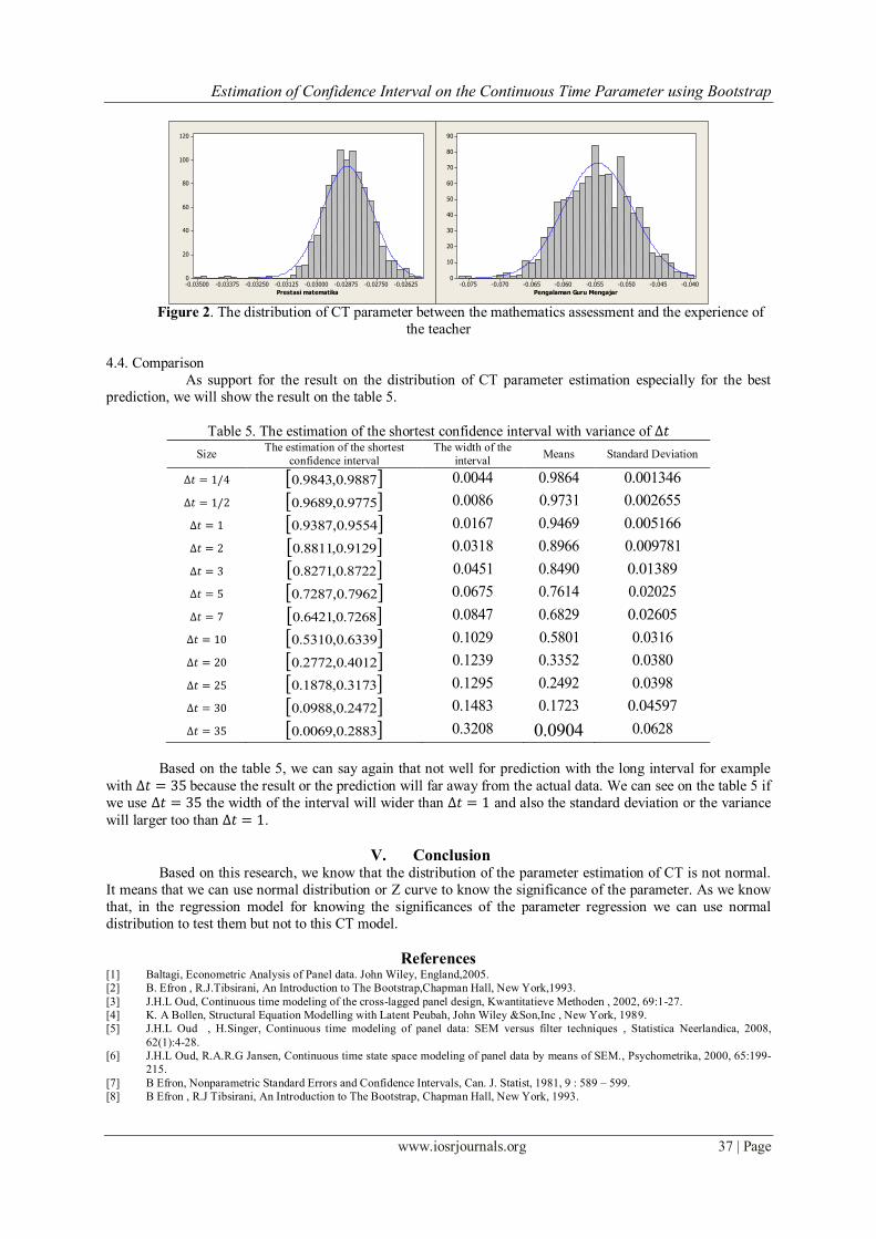
Figure 2. The distribution of CT parameter between the mathematics assessment and the experience of

the teacher

4.4. Comparison

As support for the result on the distribution of CT parameter estimation especially for the best

prediction, we will show the result on the table 5.

Table 5. The estimation of the shortest confidence interval with variance of ∆𝑡

Size The estimation of the shortest

confidence interval

The width of the

interval Means Standard Deviation

∆𝑡 = 1/4 9887.0,9843.0 0044.0

9864.0

001346.0

∆𝑡 = 1/2 9775.0,9689.0 0086.0

9731.0

002655.0

∆𝑡 = 1 9554.0,9387.0

0167.0

9469.0

005166.0

∆𝑡 = 2 9129.0,8811.0 0318.0

8966.0

009781.0

∆𝑡 = 3 8722.0,8271.0 0451.0

8490.0

01389.0

∆𝑡 = 5 7962.0,7287.0 0675.0

7614.0

02025.0

∆𝑡 = 7 7268.0,6421.0

0847.0

6829.0

02605.0

∆𝑡 = 10 6339.0,5310.0 1029.0

5801.0

0316.0

∆𝑡 = 20 4012.0,2772.0 1239.0

3352.0

0380.0

∆𝑡 = 25 3173.0,1878.0 1295.0

2492.0

0398.0

∆𝑡 = 30 2472.0,0988.0 1483.0

1723.0

04597.0

∆𝑡 = 35 2883.0,0069.0 3208.0

0904.0

0628.0

Based on the table 5, we can say again that not well for prediction with the long interval for example

with ∆𝑡 = 35 because the result or the prediction will far away from the actual data. We can see on the table 5 if

we use ∆𝑡 = 35 the width of the interval will wider than ∆𝑡 = 1 and also the standard deviation or the variance

will larger too than ∆𝑡 = 1.

V. Conclusion Based on this research, we know that the distribution of the parameter estimation of CT is not normal.

It means that we can use normal distribution or Z curve to know the significance of the parameter. As we know

that, in the regression model for knowing the significances of the parameter regression we can use normal

distribution to test them but not to this CT model.

References [1] Baltagi, Econometric Analysis of Panel data. John Wiley, England,2005.

[2] B. Efron , R.J.Tibsirani, An Introduction to The Bootstrap,Chapman Hall, New York,1993.

[3] J.H.L Oud, Continuous time modeling of the cross-lagged panel design, Kwantitatieve Methoden , 2002, 69:1-27.

[4] K. A Bollen, Structural Equation Modelling with Latent Peubah, John Wiley &Son,Inc , New York, 1989.

[5] J.H.L Oud , H.Singer, Continuous time modeling of panel data: SEM versus filter techniques , Statistica Neerlandica, 2008,

62(1):4-28.

[6] J.H.L Oud, R.A.R.G Jansen, Continuous time state space modeling of panel data by means of SEM., Psychometrika, 2000, 65:199-

215.

[7] B Efron, Nonparametric Standard Errors and Confidence Intervals, Can. J. Statist, 1981, 9 : 589 – 599.

[8] B Efron , R.J Tibsirani, An Introduction to The Bootstrap, Chapman Hall, New York, 1993.