Estimation and Inference with a (Nearly) Singular Jacobian∗

Sukjin Han

Department of Economics

University of Texas at Austin

sukjin.han@austin.utexas.edu

Adam McCloskey

Department of Economics

University of Colorado at Boulder

adam.mccloskey@colorado.edu

First Draft: February 15, 2014

This Draft: April 19, 2019

Abstract

This paper develops extremum estimation and inference results for nonlinear models with

very general forms of potential identification failure when the source of this identification

failure is known. We examine models that may have a general deficient rank Jacobian in

certain parts of the parameter space. When identification fails in one of these models, it

becomes under-identified and the identification status of individual parameters is not gener-

ally straightforward to characterize. We provide a systematic reparameterization procedure

that leads to a reparametrized model with straightforward identification status. Using this

reparameterization, we determine the asymptotic behavior of standard extremum estimators

and Wald statistics under a comprehensive class of parameter sequences characterizing the

strength of identification of the model parameters, ranging from non-identification to strong

identification. Using the asymptotic results, we propose hypothesis testing methods that

make use of a standard Wald statistic and data-dependent critical values, leading to tests

with correct asymptotic size regardless of identification strength and good power properties.

Importantly, this allows one to directly conduct uniform inference on low-dimensional func-

tions of the model parameters, including one-dimensional subvectors. The paper illustrates

these results in three examples: a sample selection model, a triangular threshold crossing

model and a collective model for household expenditures.

∗The authors are grateful to Donald Andrews, Isaiah Andrews, Xiaohong Chen, Xu Cheng, Gregory Cox,Aureo de Paula, Stephen Donald, Bruce Hansen, Bo Honore, Tassos Magdalinos, Peter Phillips, Eric Renault,Jesse Shapiro, James Stock, Yixiao Sun, Elie Tamer, Edward Vytlacil and four anonymous referees for helpfulcomments. This paper is developed from earlier work by Han (2009). The second author gratefully acknowledgessupport from the NSF under grant SES-1357607.

Keywords: Reparameterization, deficient rank Jacobian, asymptotic size, uniform inference,

subvector inference, extremum estimators, identification, nonlinear models, Wald test, weak

identification, under-identification.

JEL Classification Numbers: C12, C15.

1 Introduction

Many models estimated by applied economists suffer the problem that, at some points in the

parameter space, the model parameters lose point identification. It is often the case that at

these points of identification failure, the identified set for each parameter is not characterized by

the entire parameter space it lies in but rather the identified set for the entire parameter vector

is characterized by a lower-dimensional manifold inside of the vector’s parameter space. Such

a non-identification scenario is sometimes referred to as “under-identification” or “partial iden-

tification”. The non-identification status of these models is not straightforwardly characterized

in the sense that one cannot say that some parameters are “completely” unidentified while the

others are identified. Instead, it can be characterized by a non-identification curve that describes

the lower-dimensional manifold defining the identified set. Moreover, in practice the model pa-

rameters may be weakly identified in the sense that they are near the under-identified/partially-

identified region of the parameter space relative to the number of observations and sampling

variability present in the data.

This paper develops estimation and inference results for nonlinear models with very general

forms of potential identification failure when the source of this identification failure is known.

We characterize (global) identification failure in this paper through the Jacobian matrix of the

model restrictions: the Jacobian matrix of the model restrictions has deficient column rank in a

(typically linear) subspace of the entire parameter space.1 We examine models for which a vector

of parameters governs the identification status of the model, with identification failure occurring

when this vector of parameters is equal to a specific value. The contributions of this paper are

threefold. First, we provide a systematic reparameterization procedure that nonlinearly trans-

forms a model’s parameters into a new set of parameters that have straightforward identification

status when identification fails. Second, using this reparameterization, we derive limit theory

for a class of standard extremum estimators (e.g., generalized method of moments, minimum

distance and some forms of maximum likelihood) and Wald statistics for these models under a

comprehensive class of identification strengths including non-identification, weak identification

and strong identification. We find that the asymptotic distributions derived under certain se-

quences of data-generating processes (DGPs) indexed by the sample size provide much better

1See Rothenberg (1971) for a discussion of local vs. global identification.

1

approximations to the finite sample distributions of these objects than those derived under the

standard limit theory that assumes strong identification. Third, we use the limit theory derived

under weak identification DGP sequences to construct data-dependent critical values (CVs) for

Wald statistics that yield (uniformly) correct asymptotic size and good power properties. Im-

portantly, our robust inference procedures allow one to directly conduct hypothesis tests for

low-dimensional functions of the model parameters, including one-dimensional subvectors, that

are uniformly valid regardless of identification strength.

A substantial portion of the recent econometrics literature has been devoted to studying

estimation in the presence of weak identification and developing inference tools that are robust

to the identification strength of the parameters in an underlying economic or statistical model.

Earlier papers in this line of research focus upon the linear instrumental variables (IV) model, the

behavior of standard estimators and inference procedures under weak identification of this model

(e.g., Staiger and Stock, 1997), and the development of new inference procedures robust to the

strength of identification in this model (e.g., Kleibergen, 2002 and Moreira, 2003). More recently,

focus has shifted to nonlinear models, such as those defined through moment restrictions. In

this more general setting, researchers have similarly characterized the behavior of standard

estimators and inference procedures under various forms of weak identification (e.g., Stock and

Wright, 2000) and developed robust inference procedures (e.g., Kleibergen, 2005). Most papers

in this literature, such as Stock and Wright (2000) and Kleibergen (2005), focus upon special

cases of identification failure and weak identification by explicitly specifying how the Jacobian

matrix of the underlying model could become (nearly) singular. For example, Kleibergen (2005)

focuses on a zero rank Jacobian as the point of identification failure in moment condition models.

In this case, the identified set becomes the entire parameter space at points of identification

failure. The recent works of Andrews and Cheng (2012, 2013, 2014) implicitly focus on models

for which the Jacobian of the model restrictions has columns of zeros at points of identification

failure. For these types of models, some parameters become “completely” unidentified (those

corresponding to the zero columns) while others remain strongly identified. In this paper, we

do not restrict the form of singularity in the Jacobian at the point of identification failure. This

complicates the analysis but allows us to cover many more economic models used in practice

such as sample selection models, treatment effect models with endogenous treatment, nonlinear

regression models, nonlinear IV models, certain dynamic stochastic general equilibrium (DSGE)

models and structural vector autoregressions (VARs) identified by instruments or conditional

heteroskedasticity. Indeed, this feature of a singular Jacobian without zero columns at points of

identification failure is typical of many nonlinear models.

Only very recently have researchers begun to develop inference procedures that are robust

2

to completely general forms of (near) rank-deficiency in the Jacobian matrix. See Andrews

and Mikusheva (2016b) in the context of minimum distance (MD) estimation and Andrews and

Guggenberger (2018) and Andrews and Mikusheva (2016a) in the context of moment condi-

tion models. Andrews and Mikusheva (2016b) provide methods to directly perform uniformly

valid subvector inference while Andrews and Guggenberger (2018) and Andrews and Mikusheva

(2016a) do not.2 Unlike these papers, but like Andrews and Cheng (2012, 2013, 2014), we focus

explicitly on models for which the source of identification failure (a finite-dimensional param-

eter) is known to the researcher. This enables us to directly conduct subvector inference in a

large class of models that is not nested in the setup of Andrews and Mikusheva (2016b). Also

unlike these papers, but like Andrews and Cheng (2012, 2013, 2014), we derive nonstandard

limit theory for standard estimators and test statistics. This nonstandard limit theory sheds

light on how (badly) the standard Gaussian and chi-squared distributional approximations can

fail in practice. For example, one interesting feature of the models we study here is that the

asymptotic size of standard Wald tests for the full parameter vector (and certain subvectors) is

equal to one no matter the nominal level of the test. This feature emerges from observing that

the Wald statistic diverges to infinity under certain DGP sequences admissible under the null

hypothesis.

Aside from those already mentioned, there are many papers in the literature that study var-

ious types of under-identification in different contexts. For example, Sargan (1983) studies re-

gression models that are nonlinear in parameters and first-order locally under-identified. Phillips

(1989) and Choi and Phillips (1992) study under-identified simultaneous equations models and

spurious time series regressions. In a rather different context, Lee and Chesher (1986) also make

use of a reparameterization for a type of identification problem. Arellano et al. (2012) proposes

a way to test for under-identification in a generalized method of moments (GMM) context. Qu

and Tkachenko (2012) study under-identification in the context of DSGE models. Escanciano

and Zhu (2013) study under-identification in a class of semi-parametric models.3 Dovonon and

Renault (2013) uncover an interesting result that, when testing for common sources of condi-

tional heteroskedasticity in a vector of time series, there is a loss of first-order identification

under the null hypothesis while the model remains second-order identified. Although all of

these papers study under-identification of various forms, none of them deal with the empirically

2Andrews and Mikusheva (2016a) provide a method of “concentrating out” strongly identified nuisance pa-rameters for subvector inference when all potentially weakly identified parameters are included in the subvector.One may also “indirectly” perform subvector inference using the methods of either Andrews and Guggenberger(2018) or Andrews and Mikusheva (2016a) by using a projection or Bonferroni bound-based approach but thesemethods are known to often suffer from severe power loss. We refer the interested reader to Remark 5.2 for furthercomparisons with the methods in these papers as well as Andrews and Mikusheva (2016b).

3Both Qu and Tkachenko (2012) and Escanciano and Zhu (2013) use the phrase “conditional identification”to refer to “under-identification” as we use it here.

3

relevant potential for near or local to under-identification, one of the main focuses of the present

paper.

In order to derive our asymptotic results under a comprehensive class of identification

strengths, we begin by providing a general recipe for reparameterizing the extremum estimation

problem so that, after reparameterization, it falls under the framework of Andrews and Cheng

(2012) (AC12 hereafter). More specifically, the reparameterization procedure involves solving a

system of differential equations so that a set of the derivatives of the function that generates the

reparameterization are in the null space of the Jacobian of the original model restrictions. This

reparameterization generates a Jacobian of transformed model restrictions with zero columns at

points of identification failure. This systematic approach to nonlinear reparameterization gen-

eralizes some antecedents in linear models for which the reparameterizations amount to linear

rotations (e.g., Phillips, 1989). We show that the reparametrized extremum objective function

satisfies a crucial assumption of AC12: at points of identification failure, it does not depend

upon the unidentified parameters.4 This allows us to use the results of AC12 to find the limit

theory for the reparametrized parameter estimates. Though beyond the scope of the current

paper, our reparameterization procedure may similarly be useful as a step toward using the

general limit theory of Cox (2018) for some problems. This latter paper studies other, more

complicated forms of weak identification not covered by AC12.

We subsequently derive the limit theory for the original parameter estimates of economic

interest using the fact that they are equal to a bijective function of the reparametrized parame-

ter estimates. To obtain a full asymptotic characterization of the original parameter estimator,

we rotate its subvectors in different directions of the parameter space. The subvector estimates

converge at different rates in different directions of the parameter space when identification is

not strong, with some directions leading to a standard parametric rate of convergence and oth-

ers leading to slower rates. Under weak identification, some directions of the weakly identified

part of the parameter are not consistently estimable, leading to inconsistency in the parameter

estimator that is reflected in finite sample simulation results and our derived asymptotic approx-

imations. The rotation technique we use in our asymptotic derivations has many antecedents

in the literature. For example, Sargan (1983), Phillips (1989) and Choi and Phillips (1992) use

similar rotations to derive limit theory for estimators under identification failure; Antoine and

Renault (2009, 2012) use similar rotations to derive limit theory for estimators under “nearly-

weak” identification;5 Andrews and Cheng (2014) (AC14 hereafter) use similar rotations to find

the asymptotic distributions of Wald statistics under weak and nearly-strong identification; and

recently Phillips (2016) uses similar rotations to find limit theory for regression estimators in

4This corresponds to Assumption A of AC12.5In this paper, we follow AC12 and describe such parameter sequences as “nearly-strong”.

4

the presence of near-multicollinearity in regressors. However, unlike their predecessors used

for specific linear models, our nonlinear reparameterizations are not generally equivalent to the

rotations we use to derive asymptotic theory.

We also derive the asymptotic distributions of standard Wald statistics for general (possibly

nonlinear) hypotheses under a comprehensive class of identification strengths. The nonstan-

dard nature of these limit distributions implies that using standard quantiles from chi-squared

distributions as CVs leads to asymptotic size-distortions. To overcome this issue, we provide

two data-driven methods to construct CVs for standard Wald statistics that lead to tests with

correct asymptotic size, regardless of identification strength. The first is a direct analog of the

Type 1 Robust CVs of AC12. The second is a modified version of the adjusted-Bonferroni CVs

of McCloskey (2017), where the modifications are designed to ease the computation of the CVs

in the current setting of this paper. The former CV construction method is simpler to compute

while the latter yields better finite-sample properties. We then briefly analyze the power perfor-

mance of one of our proposed robust Wald tests in a triangular threshold crossing model with a

dummy endogenous variable. Finally, we apply the testing method in an empirical example that

analyzes the effects of educational attainment on criminal activity. The theoretical results of this

paper are based upon widely applicable high-level assumptions. We verify these assumptions for

the triangular threshold crossing model by imposing lower-level conditions in Online Appendix

B.

The paper is organized as follows. In the next section, we introduce the general class of

models subject to under-identification that we study and detail four examples of models in

this class. Section 3 introduces a new method of systematic nonlinear reparameterization that

leads to straightforward identification status under identification failure. This section includes

a step-by-step algorithm for obtaining the reparameterization. Section 4 provides the limit

theory for a general class of extremum estimators of the original model parameters under a

comprehensive class of identification strengths. The nonstandard limit distributions derived here

provide accurate approximations to the finite sample distributions of the parameter estimators,

uncovered via Monte Carlo simulation. Section 5 similarly provides the analogous limit theory

for standard Wald statistics. We describe how to perform uniformly robust inference in Section

6. Section 7 contains further details for a triangular threshold crossing model, including Monte

Carlo simulations demonstrating how well the nonstandard limit distributions derived in Sections

4–5 approximate their finite-sample counterparts and an analysis of the power properties of a

robust Wald test. Section 8 contains the empirical application. Proofs of the main results of

the paper and verification of assumptions for the threshold crossing model are contained in the

online appendix, while figures are collected at the end of the document. In addition, some of

5

the assumptions and expressions from AC12 that also appear in this paper are collected for the

reader’s convenience in The Appendix at the end of the paper.

Notationally, we respectively let bj , bj and db denote the jth entry, the jth subvector and the

dimension of a generic parameter vector b. All vectors in the paper are column vectors. However,

to simplify notation, we occasionally abuse it by writing (c, d) instead of (c′, d′)′, (c′, d)′ or (c, d′)′

for vectors c and d and for a function f(a) with a = (c, d), we sometimes write f(c, d) rather

than f(a). Finally, we write “wp1” as shorthand for “with probability one”.

2 General Class of Models

Suppose that an economic model implies a relationship among the components of a finite-

dimensional parameter θ:

0 = g(θ;γ∗) ≡ g∗(θ) ∈ Rdg (2.1)

when θ = θ∗. The “model restriction” function describing this relationship g may depend on the

true underlying parameter γ∗ that contains θ∗, i.e., the true underlying DGP. The parameter

γ∗ can be infinite-dimensional so that, e.g., moment conditions may constitute (some of) the

model restrictions. A special case of (2.1) occurs when g relates a structural parameter θ to a

reduced-form parameter ξ and depends on γ∗ only through the true value ξ∗ of ξ:

0 = g∗(θ) = ξ∗ − g(θ) ∈ Rdg (2.2)

when θ = θ∗; see Example 2.3 below.

Often, econometric models imply a decomposition of θ: θ = (β,µ), where the parameter β

determines the “identification status” of µ. That is, when β 6= β for some β, µ is identified; when

β = β, µ is under-identified; and when β is “close” to β relative to sampling variability, µ is local-

to-under-identified. For convenience and without loss of generality, we use the normalization β =

0. In this paper, we characterize identification of µ via the Jacobian of the model restrictions:

J∗(θ) ≡ ∂g∗(θ)

∂µ′. (2.3)

The Jacobian J∗(θ) will have deficient rank across the subset of the parameter space for θ for

which β = 0 but full rank over the remainder of the parameter space.6 We are considering

models that become globally under-identified in a (typically linear) subspace of the parameter

space. Our main focus is on models for which the column rank of J∗(θ) lies strictly between 0

6Assumption ID below is related to the former, and Assumption B3(iii) in AC12, which we assume later,implies the latter.

6

and dµ when β = 0 and this rank-deficiency is not the consequence of zero columns in J∗(θ);

see Remark 3.1 below for a related discussion in terms of the information matrix. Although

our results cover cases for which J∗(θ) has columns of zeros when β = 0, these cases are not of

primary interest for this paper since they are nested in the framework of AC12.

We detail four examples that have a deficient rank Jacobian (2.3) with nonzero columns

when β = 0. The first two and last examples fall into the framework of (2.1) and the third into

(2.2).

Remark 2.1. For some models, we can further decompose θ into θ = (β,µ) = (β, ζ,π), where

only the identification status of the subvector parameter π of µ is affected by the value of β.

More formally, when β = 0, rank (∂g∗(θ)/∂π′) < dπ for all θ = (0, ζ,π) ∈ Θ and γ∗ ∈ Γ,

where Θ and Γ denote the parameter spaces of θ and γ. Modulo the reordering of the elements

of µ, we can formalize the decomposition µ = (ζ,π) as follows: π is the smallest subvector of

µ such that

dπ − rank(∂g∗(θ)/∂π′

)= dµ − rank(J∗(θ))

when β = 0. That is, the rank deficiency of the Jacobian with respect to the subvector π is equal

to the rank deficiency of the Jacobian with respect to the vector µ when β = 0. This feature

holds for Examples 2.1–2.3 below, and will be illustrated as a special case throughout the paper.

Example 2.1 (Sample selection models using the control function approach).

Yi = X ′iπ1 + εi, Di = 1[ζ + Z ′1iβ ≥ νi],

(εi, νi)′ ∼ Fεν(ε, ν;π2),

where Xi ≡ (1, X ′1i)′ is k × 1, Zi ≡ (1, Z ′1i)

′ is l × 1, the variables (Xi, Zi) are independent of

the errors (εi, νi) and (Xi, Zi, εi, νi) are iid. Note that Zi may include (components of) Xi. We

observe Wi = (DiYi, Di, Xi, Zi) and Fεν(·, ·;π2) is a parametric distribution of the unobservable

variables (ε, ν) parameterized by the scalar π2. The mean and variance of each unobservable

is normalized to be zero and one, respectively. Constructing a moment condition based on the

control function approach (Heckman, 1979), we have, when θ = θ∗,

0 =g∗(θ) = Eγ∗ϕ(Wi,θ),

where θ = (β, ζ,π1,π2) and the moment function is

ϕ(w,θ) =

d

[x

q(ζ + z′1β;π2)

] [y − x′π1 − q(ζ + z′1β;π2)

]q(ζ + z′1β;π2)F−1

ν (−ζ − z′1β) [d− Fν(ζ + z′1β)] z

, (2.4)

7

with w = (dy, d, x, z) being a realization of Wi and q(·;π2) being a known function. When

Fεν(ε, ν;π2) is a bivariate standard normal distribution with correlation coefficient π2, we have

Fν(·) = Φ(·) and q(·;π2) = π2q(·) where q(·) = φ(·)/Φ(·) is the inverse Mill’s ratio based on the

standard normal density and distribution functions φ(·) and Φ(·).

Example 2.2 (Models of potential outcomes with endogenous treatment).

Y1i = X ′iπ1 + ε1i,

Y0i = X ′iπ2 + ε0i,

Di = 1[ζ + Z ′1iβ ≥ νi],

Yi = DiY1i + (1−Di)Y0i,

(ε1i, ε0i, νi)′ ∼ Fε1,ε0,ν(ε1, ε0, ν;π3),

where Fε1,ε0,ν(·, ·, ·;π3) is a parametric distribution of the unobserved variables (ε1, ε0, ν) pa-

rameterized by vector π3. We observe Wi = (Yi, Di, Xi, Zi). The Roy model (Heckman and

Honore, 1990) is a special case of this model of regime switching. This model extends the model

in Example 2.1, but is similar in the aspects that this paper focuses upon.

Example 2.3 (Threshold crossing models with a dummy endogenous variable).

Yi = 1[π1 + π2Di − εi ≥ 0]

Di = 1[ζ + βZi − νi ≥ 0], (εi, νi)

′ ∼ Fεν(εi, vi;π3).

where Zi ∈ 0, 1. We observe an iid sample of Wi = (Yi, Di, Zi) and assume that the in-

strument Zi is independent of (εi, νi). The model can be generalized by including common

exogenous covariates Xi in both equations and allowing the instrument Zi to take more than

two values. We focus on this stylized version of the model in this paper for simplicity only.

With Fεν(ε, ν;π3) = Φ(ε, ν;π3), a bivariate standard normal distribution with correlation co-

efficient π3, the model becomes the usual bivariate probit model. A more general model with

Fεν(ε, ν;π3) = C(Fε(ε), Fν(ν);π3), for C(·, ·;π3) in a class of single parameter copulas, is con-

sidered in Han and Vytlacil (2017), whose generality we follow here. Let π2 ≡ π1 + π2 and,

for simplicity, let Fν and Fε be uniform distributions.7 The results of Han and Vytlacil (2017)

provide that when θ = θ∗, ξ∗ − g(θ) = 0, where ξ = (p11,0, p11,1, p10,0, p10,1, p01,0, p01,1)′ with

7This normalization is not necessary and is only introduced here for simplicity; see Han and Vytlacil (2017)for the formulation of the identification problem without it.

8

pyd,z ≡ Prγ [Y = y,D = d|Z = z] and

g(θ) =

p11,0(θ)

p11,1(θ)

p10,0(θ)

p10,1(θ)

p01,0(θ)

p01,1(θ)

≡

C(π2, ζ;π3)

C(π2, ζ + β;π3)

π1 − C(π1, ζ;π3)

π1 − C(π1, ζ + β;π3)

ζ − C(π2, ζ;π3)

ζ + β − C(π2, ζ + β;π3)

. (2.5)

For later use, we also define the (redundant) probabilities:

p00,0(θ) ≡ 1− p11,0(θ)− p10,0(θ)− p01,0(θ), (2.6)

p00,1(θ) ≡ 1− p11,1(θ)− p10,1(θ)− p01,1(θ).

Example 2.4 (Engel curve models for household share). Tommasi and Wolf (2018) discuss

Engel curve estimation for the private assignable good in the Dunbar et al. (2013) collective

model for household expenditure shares when using the PIGLOG utility function. See equation

(2) of Tommasi and Wolf (2018) for these Engel curves. These authors estimate the model

parameters by a particular nonlinear least squares criterion. We instead consider the general

GMM estimation problem in this context for which 0 = g∗(θ) = Eγ∗ϕ(Wi,θ) when θ = θ∗,

where θ = (β,π1,π2,π3) and the moment function is

ϕ(w,θ) = A(yh)

[(w1,h

w2,h

)−

(π1(π2 + π3 + β log(π1yh))

(1− π1)(π2 + β log((1− π1)yh))

)], (2.7)

where A(·) is some (dg × 2)-dimensional function. For example,

A(yh) =

1 0

yh 0

0 1

0 yh

.

There are many other examples of models that fit our framework including but not limited

to nonlinear IV models, nonlinear regression models, certain DSGE models and structural VARs

identified by conditional heteroskedasticity or instruments.

Examples 2.1 and 2.2 are contained in a class of moment condition models that uses a

control function approach to account for endogeneity. This class of models fits our framework

9

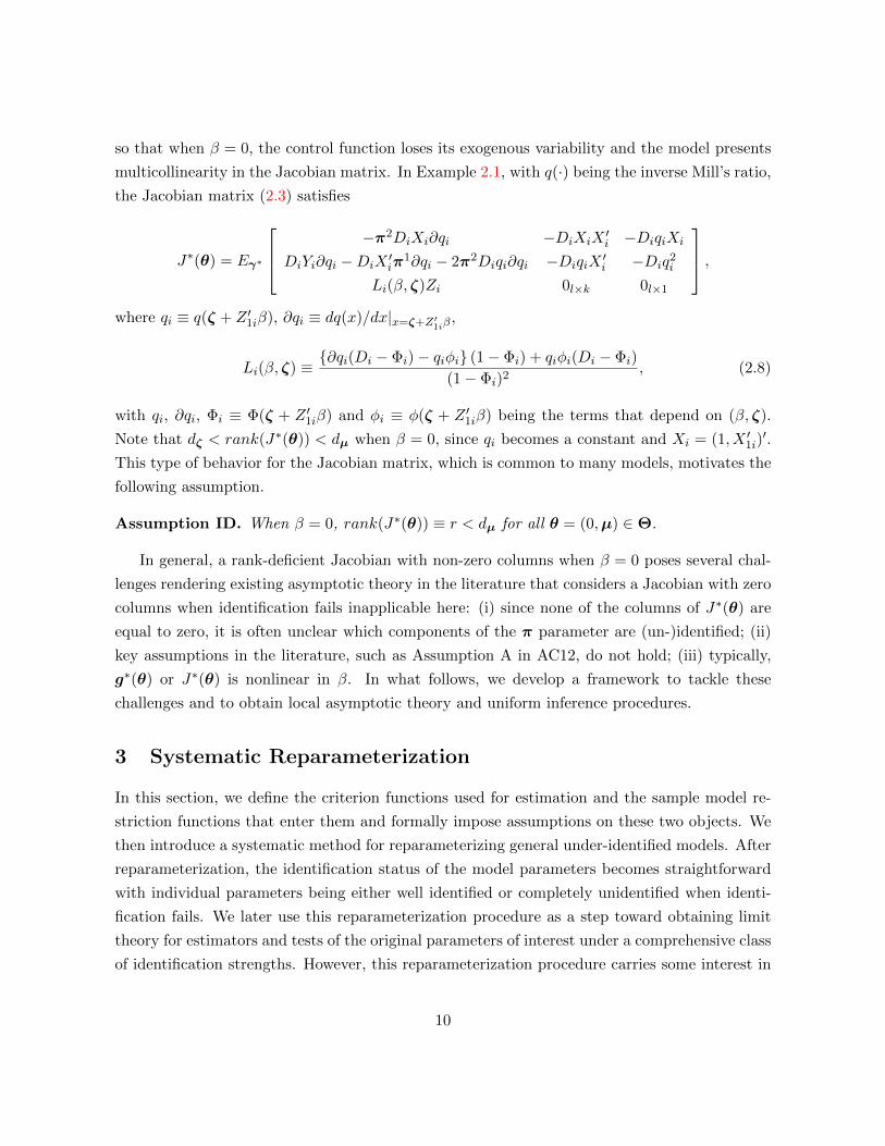
so that when β = 0, the control function loses its exogenous variability and the model presents

multicollinearity in the Jacobian matrix. In Example 2.1, with q(·) being the inverse Mill’s ratio,

the Jacobian matrix (2.3) satisfies

J∗(θ) = Eγ∗

−π2DiXi∂qi −DiXiX′i −DiqiXi

DiYi∂qi −DiX′iπ

1∂qi − 2π2Diqi∂qi −DiqiX′i −Diq

2i

Li(β, ζ)Zi 0l×k 0l×1

,where qi ≡ q(ζ + Z ′1iβ), ∂qi ≡ dq(x)/dx|x=ζ+Z′1iβ

,

Li(β, ζ) ≡ ∂qi(Di − Φi)− qiφi (1− Φi) + qiφi(Di − Φi)

(1− Φi)2, (2.8)

with qi, ∂qi, Φi ≡ Φ(ζ + Z ′1iβ) and φi ≡ φ(ζ + Z ′1iβ) being the terms that depend on (β, ζ).

Note that dζ < rank(J∗(θ)) < dµ when β = 0, since qi becomes a constant and Xi = (1, X ′1i)′.

This type of behavior for the Jacobian matrix, which is common to many models, motivates the

following assumption.

Assumption ID. When β = 0, rank(J∗(θ)) ≡ r < dµ for all θ = (0,µ) ∈ Θ.

In general, a rank-deficient Jacobian with non-zero columns when β = 0 poses several chal-

lenges rendering existing asymptotic theory in the literature that considers a Jacobian with zero

columns when identification fails inapplicable here: (i) since none of the columns of J∗(θ) are

equal to zero, it is often unclear which components of the π parameter are (un-)identified; (ii)

key assumptions in the literature, such as Assumption A in AC12, do not hold; (iii) typically,

g∗(θ) or J∗(θ) is nonlinear in β. In what follows, we develop a framework to tackle these

challenges and to obtain local asymptotic theory and uniform inference procedures.

3 Systematic Reparameterization

In this section, we define the criterion functions used for estimation and the sample model re-

striction functions that enter them and formally impose assumptions on these two objects. We

then introduce a systematic method for reparameterizing general under-identified models. After

reparameterization, the identification status of the model parameters becomes straightforward

with individual parameters being either well identified or completely unidentified when identi-

fication fails. We later use this reparameterization procedure as a step toward obtaining limit

theory for estimators and tests of the original parameters of interest under a comprehensive class

of identification strengths. However, this reparameterization procedure carries some interest in

10

its own right because it (i) characterizes the submanifold of the original parameter space that

is (un)identified and (ii) has the potential for application to finding the limit theory for general

models that are globally under-identified across their entire parameter space (in contrast to

those that lose identification in the subspace for which β = 0).

We define the extremum estimator θn as the minimizer of the criterion function Qn(θ) over

the optimization parameter space Θ:

θn ∈ Θ and Qn(θn) = infθ∈Θ

Qn(θ) + o(n−1).

In the following assumptions we presume that Qn(θ) is a function of θ only through the sample

counterpart gn(θ) of g∗(θ). In the case of MD and some particular maximum likelihood (ML)

models, gn(θ) = ξn − g(θ), where ξn is a sample analog of ξ∗, in analogy to (2.2). For GMM,

gn(θ) = n−1∑n

i=1 ϕ(Wi,θ).

Assumption CF. Qn(θ) can be written as

Qn(θ) = Ψn(gn(θ))

for some random function Ψn(·) that is differentiable wp1.

Assumption CF is naturally satisfied when we construct GMM/MD or ML criterion func-

tions, given (2.1) or (2.2). Note that models that generate minimum distance structures and

certain types of likelihoods as in Example 2.3 involve g∗(θ) = ξ∗−g(θ) by (2.2). For a GMM/MD

criterion function, Ψn(gn(θ)) = ‖Wngn(θ)‖2 where Wn is a (possibly random) weight matrix.8

Note also that our framework includes general ML estimation with concave likelihoods, since it

is numerically equivalent to GMM estimation that uses the score equations as moments.

Assumption Reg1. gn : Θ→ Rdg is continuously differentiable in θ wp1.

To simplify the asymptotic theory derived in Section 4, we impose the following assumption

that ensures the reparameterization function h(·) in Procedure 3.1 below does not depend on

the true DGP.

Assumption Jac. When β = 0, the null space of J∗(θ) is a subspace of the null space of

∂gn(θ)/∂µ′ wp1 for all n ≥ 1. The null space of J∗(θ) does not depend upon the true DGP γ∗.

We allow the null space of the sample Jacobian to be larger than that of the population

Jacobian to accommodate the possibility that particular realizations of the random variables

8Note that Assumption CF does not cover GMM with a continuously updating weight matrix Wn(θ).

11

entering the sample Jacobian can induce additional rank reduction. For example, this allows

the random variables X1i in Example 2.1 above to equal zero for all i = 1, . . . , n. Examples

2.1–2.4 satisfy this assumption. However, the asymptotic theory derived in Section 4 can be

extended to some cases for which our reparameterization is DGP-dependent, but we have not

found an application for which such an extension would be useful.

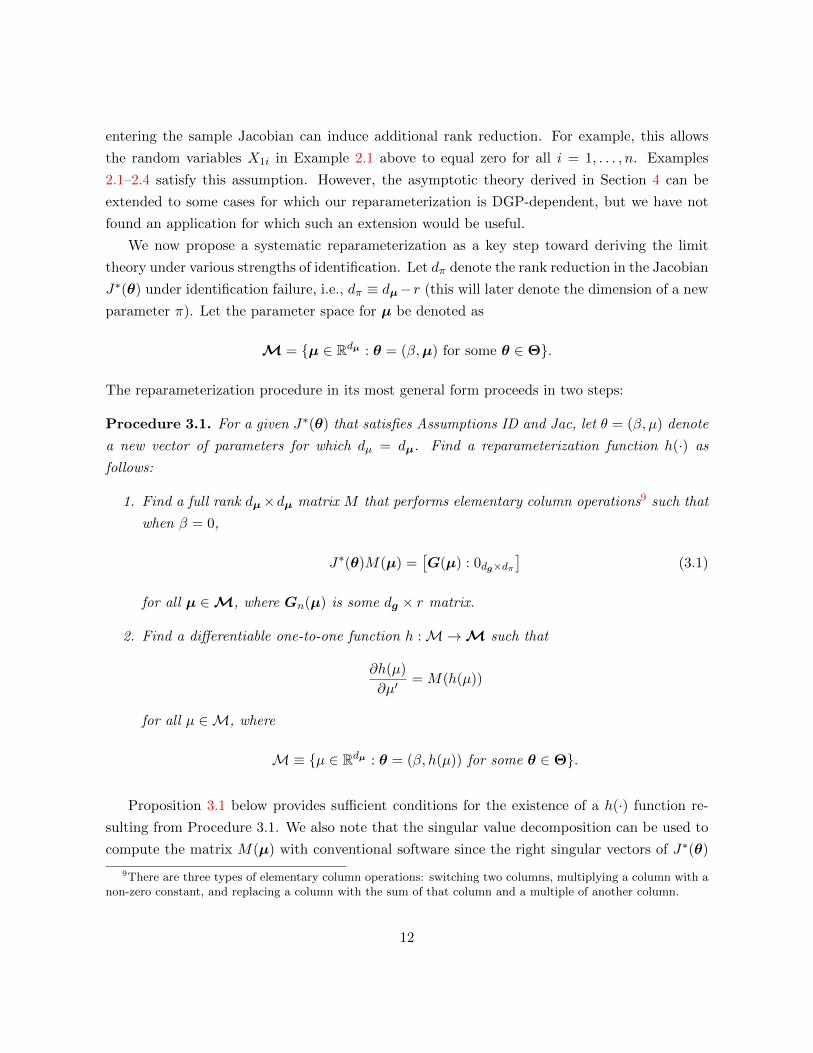
We now propose a systematic reparameterization as a key step toward deriving the limit

theory under various strengths of identification. Let dπ denote the rank reduction in the Jacobian

J∗(θ) under identification failure, i.e., dπ ≡ dµ−r (this will later denote the dimension of a new

parameter π). Let the parameter space for µ be denoted as

M = µ ∈ Rdµ : θ = (β,µ) for some θ ∈ Θ.

The reparameterization procedure in its most general form proceeds in two steps:

Procedure 3.1. For a given J∗(θ) that satisfies Assumptions ID and Jac, let θ = (β, µ) denote

a new vector of parameters for which dµ = dµ. Find a reparameterization function h(·) as

follows:

1. Find a full rank dµ×dµ matrix M that performs elementary column operations9 such that

when β = 0,

J∗(θ)M(µ) =[G(µ) : 0dg×dπ

](3.1)

for all µ ∈M, where Gn(µ) is some dg × r matrix.

2. Find a differentiable one-to-one function h :M→M such that

∂h(µ)

∂µ′= M(h(µ))

for all µ ∈M, where

M≡ µ ∈ Rdµ : θ = (β, h(µ)) for some θ ∈ Θ.

Proposition 3.1 below provides sufficient conditions for the existence of a h(·) function re-

sulting from Procedure 3.1. We also note that the singular value decomposition can be used to

compute the matrix M(µ) with conventional software since the right singular vectors of J∗(θ)

9There are three types of elementary column operations: switching two columns, multiplying a column with anon-zero constant, and replacing a column with the sum of that column and a multiple of another column.

12

that correspond to its zero singular values span its null space and its left singular vectors that

correspond to its non-zero singular values span its column space.10 With the reparameterization

function h(·), we transform µ to µ such that µ = h(µ). That is, we have the reparameterization

as the following one-to-one map:

θ ≡ (β, µ) 7→ θ ≡ (β,µ), (3.2)

where (β,µ) = (β, h(µ)). Throughout the paper, we use boldface font for the original parameters

and standard font for the transformed parameters; once all of the relevant parameters are

introduced, we summarize the notation in Table 1. Let π denote the subvector composed of

the final dπ entries of the new parameter µ so that we may write µ = (ζ, π). We illustrate

this reparameterization approach in the following continuation of Example 2.1. The approach

is further illustrated in Examples 2.3–2.4 below.

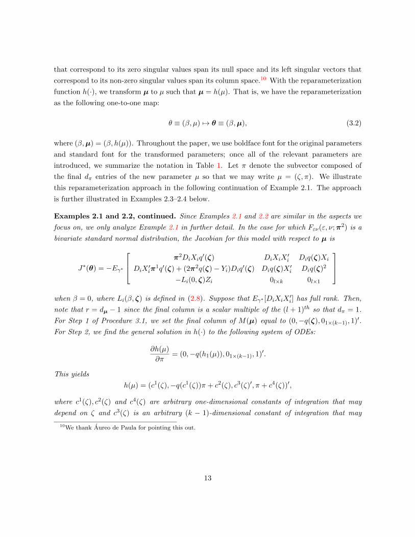
Examples 2.1 and 2.2, continued. Since Examples 2.1 and 2.2 are similar in the aspects we

focus on, we only analyze Example 2.1 in further detail. In the case for which Fεν(ε, ν;π2) is a

bivariate standard normal distribution, the Jacobian for this model with respect to µ is

J∗(θ) = −Eγ∗

π2DiXiq′(ζ) DiXiX

′i Diq(ζ)Xi

DiX′iπ

1q′(ζ) + (2π2q(ζ)− Yi)Diq′(ζ) Diq(ζ)X ′i Diq(ζ)2

−Li(0, ζ)Zi 0l×k 0l×1

when β = 0, where Li(β, ζ) is defined in (2.8). Suppose that Eγ∗ [DiXiX

′i] has full rank. Then,

note that r = dµ − 1 since the final column is a scalar multiple of the (l + 1)th so that dπ = 1.

For Step 1 of Procedure 3.1, we set the final column of M(µ) equal to (0,−q(ζ), 01×(k−1), 1)′.

For Step 2, we find the general solution in h(·) to the following system of ODEs:

∂h(µ)

∂π= (0,−q(h1(µ)), 01×(k−1), 1)′.

This yields

h(µ) = (c1(ζ),−q(c1(ζ))π + c2(ζ), c3(ζ)′, π + c4(ζ))′,

where c1(ζ), c2(ζ) and c4(ζ) are arbitrary one-dimensional constants of integration that may

depend on ζ and c3(ζ) is an arbitrary (k − 1)-dimensional constant of integration that may

10We thank Aureo de Paula for pointing this out.

13

depend on ζ. Upon setting c1(ζ) = ζ1, c2(ζ) = ζ2, c3(ζ) = (ζ3, . . . , ζk+1)′ and c4(ζ) = 0, we have

∂h(µ)

∂µ′=

1 0 01×(k−1) 0

−q′(ζ1)π 1 01×(k−1) −q(ζ1)

0(k−1)×1 0(k−1)×1 Ik−1 0(k−1)×1

0 0 01×(k−1) 1

being full rank. Thus, we have found a one-to-one reparameterization function h(·) such that

µ = (ζ,π) = h(µ) = (ζ1, ζ2 − q(ζ1)π, ζ3, . . . , ζk+1, π), or equivalently, ζ1 = ζ, ζ2 = π11 + q(ζ)π2,

(ζ3, . . . , ζk+1) = (π12, . . . ,π

1k) and π = π2.

Define the population and sample model restrictions and the criterion functions of the new

parameter θ as

g∗(θ) ≡ g∗(β, h(µ)), gn(θ) ≡ gn(β, h(µ))

and

Qn(θ) ≡ Qn(β, h(µ)).

The new Jacobian ∂g∗(θ)/∂µ′ = (∂g∗(θ)/∂µ′)(∂h(µ)/∂µ′) has the same reduced rank r < dµ =

dµ as the original Jacobian J∗(θ) = ∂g∗(θ)/∂µ′ since ∂h(µ)/∂µ = M(h(µ)) has full rank. But

now, by the construction of the reparameterization function h(·) according to Procedure 3.1, the

rank reduction arises purely from the final dπ columns of ∂g∗(θ)/∂µ′ being equal to zero. Using

this result, in conjunction with Assumption Jac, the reparametrized criterion function Qn(θ)

satisfies a property that is instrumental to deriving the limit theory detailed below.

Theorem 3.1. Under Assumptions ID, CF, Reg1 and Jac, Qn(θ) does not depend upon π when

β = 0 for all θ = (0, ζ, π) ∈ Θ.

In conjunction with other assumptions, the result of this theorem allows us to apply the

asymptotic results in Theorems 3.1 and 3.2 of AC12 to the reparametrized criterion function

Qn(θ), the new parameter θ and estimator θn, defined by

Qn(θn) = infθ∈Θ

Qn(θ) + o(n−1),

where Θ is the optimization parameter space in the reparametrized estimation problem and is

defined in terms of the original optimization parameter space Θ as follows:

Θ ≡ (β, µ) ∈ Rdθ : (β, h(µ)) ∈ Θ.

We now provide an algorithm for practical implementation of Procedure 3.1.

14

Algorithm 3.1. For a given J∗(θ) that satisfies Assumptions ID and Jac, let θ = (β, µ) =

(β, ζ, π) denote a new vector of parameters for which dµ = dµ. Find a reparameterization

function h(·) as follows:

1. Find a deterministic non-zero dµ × 1 vector m(1) such that when β = 0,

J∗(θ)m(1)(µ) = 0dg×1 (3.3)

for all µ ∈M.

2. Let µ(1) = (ζ(1), π(1)) denote a new dµ × 1 vector of parameters, where π(1) is a dπ × 1

subvector. Find the general solution in h(1) : M(1) →M to the following system of first

order ordinary differential equations (ODEs):

∂h(1)(µ(1))

∂π(1)1

= m(1)(h(1)(µ(1))) (3.4)

for all µ(1) ∈M(1) ≡ µ(1) ∈ Rdµ : θ = (β, h(1)(µ(1))) for some θ ∈ Θ.

3. From the general solution for h(1) in Step 2, find a particular solution for h(1) such that

the matrix ∂h(1)(µ(1))/∂µ(1)′ has full rank for all µ(1) ∈M(1).11

4. If dπ = 1 (i.e., π(1)1 = π(1)), stop and set h = h(1) and µ = µ(1). Otherwise, set θ(1) =

(β, µ(1)), g(1)(θ(1)) = g∗(β, h(1)(µ(1))), Θ(1) = (β, µ(1)) ∈ Rdθ : (β, h(1)(µ(1))) ∈ Θ and

i = 2 (moving to the second iteration of the algorithm) and continue to the next step.

5. Find a non-zero dµ × 1 vector m(i) such that when β = 0,

∂g(i−1)(θ(i−1))

∂µ(i−1)′m(i)(µ(i−1)) = 0dg×1 (3.5)

for all µ(i−1) ∈M(i−1).

6. Let µ(i) = (ζ(i), π(i)) denote a new dµ × 1 vector of parameters, where π(i) is a dπ × 1

subvector. Find the general solution in h(i) : M(i) → M(i−1) to the following system of

first order ODEs:∂h(i)(µ(i))

∂π(i)i

= m(i)(h(i)(µ(i))), (3.6)

11When evaluated at µ = h(1)(µ(1)), the vector m(1)(µ) is a column in the matrix ∂h(1)(µ(1))/∂µ(1)′, denotedas M (1) later. The analogous statement applies to m(i) in Steps 5–6. In the special case for which dπ = 1, m(1)(µ)evaluated at µ = h(1)(µ(1)) is equal to the final column of ∂h(1)(µ(1))/∂µ(1)′.

15

for all µ(i) ∈M(i) ≡ µ(i) ∈ Rdµ : θ(i−1) = (β, h(i)(µ(i))) for some θ(i−1) ∈ Θ(i−1).

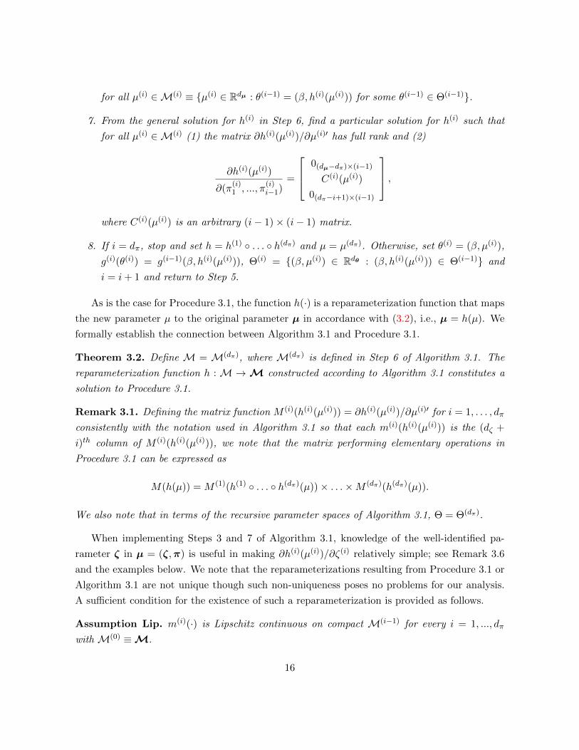
7. From the general solution for h(i) in Step 6, find a particular solution for h(i) such that

for all µ(i) ∈M(i) (1) the matrix ∂h(i)(µ(i))/∂µ(i)′ has full rank and (2)

∂h(i)(µ(i))

∂(π(i)1 , ..., π

(i)i−1)

=

0(dµ−dπ)×(i−1)

C(i)(µ(i))

0(dπ−i+1)×(i−1)

,where C(i)(µ(i)) is an arbitrary (i− 1)× (i− 1) matrix.

8. If i = dπ, stop and set h = h(1) . . . h(dπ) and µ = µ(dπ). Otherwise, set θ(i) = (β, µ(i)),

g(i)(θ(i)) = g(i−1)(β, h(i)(µ(i))), Θ(i) = (β, µ(i)) ∈ Rdθ : (β, h(i)(µ(i))) ∈ Θ(i−1) and

i = i+ 1 and return to Step 5.

As is the case for Procedure 3.1, the function h(·) is a reparameterization function that maps

the new parameter µ to the original parameter µ in accordance with (3.2), i.e., µ = h(µ). We

formally establish the connection between Algorithm 3.1 and Procedure 3.1.

Theorem 3.2. Define M = M(dπ), where M(dπ) is defined in Step 6 of Algorithm 3.1. The

reparameterization function h : M →M constructed according to Algorithm 3.1 constitutes a

solution to Procedure 3.1.

Remark 3.1. Defining the matrix function M (i)(h(i)(µ(i))) = ∂h(i)(µ(i))/∂µ(i)′ for i = 1, . . . , dπ

consistently with the notation used in Algorithm 3.1 so that each m(i)(h(i)(µ(i))) is the (dζ +

i)th column of M (i)(h(i)(µ(i))), we note that the matrix performing elementary operations in

Procedure 3.1 can be expressed as

M(h(µ)) = M (1)(h(1) . . . h(dπ)(µ))× . . .×M (dπ)(h(dπ)(µ)).

We also note that in terms of the recursive parameter spaces of Algorithm 3.1, Θ = Θ(dπ).

When implementing Steps 3 and 7 of Algorithm 3.1, knowledge of the well-identified pa-

rameter ζ in µ = (ζ,π) is useful in making ∂h(i)(µ(i))/∂ζ(i) relatively simple; see Remark 3.6

and the examples below. We note that the reparameterizations resulting from Procedure 3.1 or

Algorithm 3.1 are not unique though such non-uniqueness poses no problems for our analysis.

A sufficient condition for the existence of such a reparameterization is provided as follows.

Assumption Lip. m(i)(·) is Lipschitz continuous on compact M(i−1) for every i = 1, ..., dπ

with M(0) ≡M.

16

Proposition 3.1. Under Assumptions ID, Jac and Lip, there exists a reparametrization func-

tion h(·) on M that is an output of Algorithm 3.1 if Assumption Lip holds.

Assumption Lip is related to restrictions on g∗(θ). In practice, one can verify this assumption

by simply calculating m(i)(·) in Step 2 or 5 in Algorithm 3.1, as these steps are straightforward

to implement.

Remark 3.2. In some cases, it may be difficult to solve the ODEs (3.4) analytically. Nev-

ertheless, an abundance of numerical methods for solving systems of ODEs is readily available

in the literature.12 One can numerically solve for the h(i) functions in (3.4) using methods in,

e.g., Quarteroni et al. (2010). To summarize a standard approach to this problem, one can first

approximate the h(i) functions using known basis functions and transform the system of ODEs

into a nonlinear system of equations. Then a Newton-Raphson type method can be implemented

to solve for the coefficients on the basis functions, thus obtaining a numerical solution for the

h(i) functions. See Chapters 7–11 of Quarteroni et al. (2010) for details on the choice of basis

functions and algorithms used to implement this approach as well as other details for numerical

methods with nonlinear ODEs.

Remark 3.3. The nonlinear reparameterization approach we pursue here results in a new pa-

rameter with straightforward identification status when identification fails: ζ is well-identified

and π is completely unidentified. When β is close to zero, π will be weakly identified while (β, ζ)

remain strongly identified. Our analysis can be seen as a generalization of linear rotation-based

reparameterization approaches that have been successfully used to transform linear models in the

presence of identification failure so that the new parameters have the same straightforward iden-

tification status. See for example, Phillips (1989) and Choi and Phillips (1992) in the context of

linear IV models and Phillips (2016) in the context of the linear regression model with potential

multicollinearity.

Remark 3.4. We note that our systematic reparameterization approach may also be useful

in contexts for which a particular model is globally under-identified across its entire parameter

space (not just in the subspace for which a parameter β is equal to zero). The reparameteriza-

tion procedure may be useful for analyzing the identification properties of such models as well as

determining the limiting behavior of parameter estimates and test statistics. For models that are

globally under-identified across their parameter space with a constant (deficient) rank Jacobian,

the subsequent results of sections 4–6 could be modified so that no parameter β appears in the

analysis and the relevant limiting distributions would correspond to those derived under weak

12We thank Andres Santos for pointing this out.

17

(β,µ) = (β, h(µ)) Determines ID ID subject to failure ID not subject to failure

Original parametersβ µ,π β, ζ

θ ≡ (β,µ) ≡ (β, ζ,π)

Transformed parametersβ µ, π β, ζ

θ ≡ (β, µ) ≡ (β, ζ, π)

Table 1: Summary of Notation

identification with the localization parameter b simply set equal to zero. For example, such an

approach may be useful for under-identified DSGE models used in macroeconomics (see e.g., Ko-

munjer and Ng, 2011 and Qu and Tkachenko, 2012). Further analysis of this approach is well

beyond the scope of the present paper.

Remark 3.5. As can be seen from the continuation of Examples 2.1 and 2.3, when we know

the component ζ of µ is well-identified for all values of β, we can form h(·) so that the first

dζ elements of h(µ) are equal to the first dζ elements of the new well-identified parameter ζ =

(ζ1, ζ2), viz., ζ = (h1(µ), . . . , hdζ(µ)) = ζ1. This is the special case described in Remark 2.1. In

this special case, the reparameterization (3.2) can be written as a one-to-one map

θ ≡ (β, ζ, π) 7→ θ ≡ (β, ζ,π),

where (β, ζ,π) = (β, ζ1, h2(ζ2, π)) with µ = (ζ1, ζ2, π) = (ζ, π) and ζ is the new always well-

identified parameter.

We summarize the notation for the original and transformed parameters in Table 1 and close

this section by illustrating the reparameterization algorithm with two other examples discussed

earlier.

Example 2.3, continued. Given the specification of a single parameter copula C(·, ·;π3),

this model can be estimated by minimizing the negative (conditional) likelihood function so that

g∗(θ) = ξ∗ − g(θ), where ξ∗ is equal to a vector of the probabilities pyd,z’s and g(θ) is defined

18

in (2.5).13 The Jacobian for this model with respect to µ is

J∗(θ) = −∂g(θ)

∂µ′= −

C2(π2, ζ;π3) 0 C1(π2, ζ;π3) C3(π2, ζ;π3)

C2(π2, ζ;π3) 0 C1(π2, ζ;π3) C3(π2, ζ;π3)

−C2(π1, ζ;π3) 1− C1(π1, ζ;π3) 0 −C3(π1, ζ;π3)

−C2(π1, ζ;π3) 1− C1(π1, ζ;π3) 0 −C3(π1, ζ;π3)

1− C2(π2, ζ;π3) 0 −C1(π2, ζ;π3) −C3(π2, ζ;π3)

1− C2(π2, ζ;π3) 0 −C1(π2, ζ;π3) −C3(π2, ζ;π3)

when β = 0, where C1(·, ·;π3), C2(·, ·;π3) and C3(·, ·;π3) denote the derivatives of C(·, ·;π3)

with respect to the first argument, the second argument and π3. This matrix contains only three

linearly independent row so that r = dµ− 1. In the following analysis, since dπ = 1, we simplify

notation by letting h(1) = h, m(1) = m and µ(1) = µ = (ζ, π). For Step 1 of Algorithm 3.1, we

set m(µ) = (0, C3(π1, ζ;π3)/(1 − C1(π1, ζ;π3)),−C3(π2, ζ;π3)/C1(π2, ζ;π3), 1)′. For Step 2,

a set of general solutions to the system of ODEs

∂h(µ)

∂π=

0

C3(h2(µ),h1(µ);h4(µ))1−C1(h2(µ),h1(µ);h4(µ))

−C3(h3(µ),h1(µ);h4(µ))C1(h3(µ),h1(µ);h4(µ))

1

(3.7)

is implied by

h1(µ) = c1(ζ)

h2(µ)− C(h2(µ), h1(µ);h4(µ)) = c2(ζ) (3.8)

C(h3(µ), h1(µ);h4(µ)) = c3(ζ)

h4(µ) = π + c4(ζ),

where ci(ζ) is an arbitrary one-dimensional function of ζ for i = 1, 2, 3, 4. For Step 3, upon

13Maximizing the conditional likelihood is equivalent to maximizing the full likelihood for this problem.

19

setting c1(ζ) = ζ1, c2(ζ) = ζ2, c3(ζ) = ζ3 and c4(ζ) = 0, we have

∂h(µ)

∂µ′=

1 0 0 0

C2(h2(µ),ζ1;π)1−C1(h2(µ),ζ1;π)

11−C1(h2(µ),ζ1;π) 0 C3(h2(µ),ζ1;π)

1−C1(h2(µ),ζ1;π)

−C2(h3(µ),ζ1;π)C1(h3(µ),ζ1;π) 0 1

C1(h3(µ),ζ1;π) −C3(h3(µ),ζ1;π)C1(h3(µ),ζ1;π)

0 0 0 1

(3.9)

being full rank. Thus, we have found a reparameterization function h(·) satisfying the conditions

of Algorithm 3.1 though its explicit form will depend upon the functional form of the copula C(·).For example, if we use the Ali-Mikhail-Haq copula, defined for u1, u2 ∈ [0, 1] and π ∈ [−1, 1) by

C(u1, u2;π) =u1u2

1− π(1− u1)(1− u2), (3.10)

we obtain the following closed-form solution for h(·):

h(µ) =

ζ1

−b(µ)+√b(µ)2−4a(µ)c(µ)

2a(µ)ζ3(1−π+πζ1)ζ1−ζ3π+ζ1ζ3π

π

, (3.11)

where a(µ) = π(1 − ζ1), b(µ) = (1 − ζ1)(1 − π − πζ2) and c(µ) = ζ2[π(1 − ζ1) − 1].14 For any

choice of copula, we can also express the new parameters as a function of the original ones as

follows:

µ = (ζ1, ζ2, ζ3, π) = h−1(ζ,π) = (ζ,π1 − C(π1, ζ;π3), C(π2, ζ;π3),π3). (3.12)

Example 2.4, continued. In this example, we again consider GMM estimation so that g∗(θ) =

Eγ∗ϕ(Wi,θ), where the moment function ϕ(w,θ) is given by (2.7). The Jacobian with respect

to µ is

J∗(θ) = −Eγ∗A(Yh,i)

[π2 + π3 π1 π1

−π2 1− π1 0

]when β = 0. Since again r = dµ − 1 so that dπ = 1, simplifying notation as in the previous

examples, for Step 1 of Algorithm 3.1, we set m(µ) = (−π1(1− π1),−π1π2,π2 + π3(1− π1))′.

14As may be gleaned from this formula, the expression for h2(µ) comes from solving a quadratic equation.This solution has two solutions, one of which is always negative and one of which is always positive. Given thath2(µ) = π1 must be positive, h2(µ) is equal to the positive solution.

20

For Step 2, we need to find the general solution in h(·) to the following system of ODEs:

∂h(µ)

∂π= (−h1(µ)(1− h1(µ)),−h1(µ)h2(µ), h2(µ) + h3(µ)(1− h1(µ)))′.

Given its triangular structure, this system can be solved successively using standard single-

equation ODE methods, starting with the ∂h1(µ)/∂π equation, then the ∂h2(µ)/∂π equation,

followed by the ∂h3(µ)/∂π equation. The general solution takes the form

h(µ) =

[1 + c1(ζ)eπ]−1

c2(ζ)[e−π + c1(ζ)]

c3(ζ)[1 + c1(ζ)eπ]− c2(ζ)[e−π + c1(ζ)]

,

where ci(ζ) is an arbitrary function of ζ for i = 1, 2, 3. For Step 3, setting c1(ζ) = 1, c2(ζ) = eζ1

and c3(ζ) = ζ2 induces a simple triangular structure on the components of h(µ) as functions of

µ, i.e., so that h1(µ) is a function of π only and h2(µ) is a function of π and ζ1 only. Such a

triangular structure makes it easier to solve for µ in terms of µ. In this case, we have

∂h(µ)

∂µ′=

0 0 −eπ(1 + eπ)−2

eζ1(e−π + 1) 0 −eζ1−π

−eζ1(e−π + 1) 1 + eπ ζ2eπ + eζ1−π

being full rank. Thus, we have found a reparameterization function h(·) satisfying the conditions

of Algorithm 3.1 such that µ = h(µ) = (1/(1 + eπ), eζ1(e−π + 1), ζ2(1 + eπ) − eζ1(e−π + 1)), or

equivalently, µ = (ζ1, ζ2, π) = (log(π2(1− π1)),π1(π2 + π3), log((1− π1)/π1)).

The non-uniqueness of the reparameterizations resulting from Procedure 3.1 or Algorithm 3.1

leads to the natural question of how to “choose” the appropriate reparameterization in practice.

A natural criterion for guidance on the choice of reparameterization is interpretability. With this

criterion in mind, we recommend choosing a reparameterization function h(·) such that, after

suitable permutation of its rows and columns, ∂h(µ)/∂µ′ is triangular. The inverse function

theorem implies that (after suitable permutations) ∂h−1(µ)/∂µ′ will similarly be a triangular

matrix. This would then imply, for example, that ζ1 is a function of only one element of µ, ζ2

is a function of two or less elements of µ, and so on. This is desirable from an interpretability

perspective as it allows the user to understand which functions of the original model parameters

are identified, with the goal of keeping these functions as simple as possible. An additional

way of doing this is to choose the reparameterization function so that ∂h(µ)/∂µ′ is sparse.

Interpretability is likely to be easiest when one chooses h(·) to have both of these properties. In

21

practice, the “choice” of reparameterization is essentially dictated by the choice of constants of

integration when moving from the general solution to a system of ODEs to a particular solution,

in e.g., steps 3. and 7. of Algorithm 3.1. Note that in the illustrative reparameterizations given

for Examples 2.1, 2.3 and 2.4 above, we indeed choose the constants of integration (ci(ζ)’s and

ci(ζ)’s) following the general advice given here.

4 Limit Theory for Extremum Estimators

We proceed to derive the limit theory for the extremum estimator θn under a comprehensive

class of identification strengths by applying results from AC12 to the estimator of the parameters

in the reparametrized model θn and then determining the asymptotic behavior of the original

parameter estimator of interest via the relation θn = (βn, h(µn)). We formally characterize a

local-to-deficient rank Jacobian by modeling the β parameter as local-to-zero. This allows us

to fully characterize different strengths of identification, namely, strong, semi-strong, and weak

(which includes non-identification). Our ultimate goal from deriving asymptotic theory under

parameters with different strengths of identification is to conduct uniformly valid inference that

is robust to identification strength.

The true parameter space Γ for γ takes the form

Γ = γ = (θ, φ) : θ ∈ Θ, φ ∈ Φ(θ),

where Θ is a subset of Rdθ15 and Φ∗(θ) ⊂ Φ∗ for all θ ∈ Θ for some compact metric space Φ∗

with a metric that induces weak convergence of the bivariate distributions of the data (Wi,Wi+m)

for all i,m ≥ 1.16 We pause here to illustrate the form of this parameter space in two of our

running examples.

Examples 2.1 and 2.2, continued. We again focus upon Example 2.1 since the parameter

space for Example 2.2 has similar features. Here we also focus on the classic case for which

Fεν is a bivariate standard normal distribution. The parameter space for θ takes the form

Θ = B × Z ×Π1 ×Π2, where B =×l−1j=1[bL,j , bH,j ] with bL,j , bH,j ∈ R such that −1 < bL,j ≤

0 ≤ bH,j < 1 and bL,j 6= bH,j for j = 1, . . . , dβ, Z ⊂ R, Π1 ⊂ Rk, Π2 ⊂ (−1, 1), Z, Π1

and Π2 are compact. In this example, φ denotes the joint distribution of (Xi, Zi, εi, νi). Define

15Technically, the true parameter space for θ must be a subspace of the interior of the optimization parameterspace Θ. We suppress this distinction in the main text for ease of notation and refer the interested reader to TheAppendix for further details.

16Technically, there must exist a metric on Φ∗ such that (Wi,Wi+m) under γ converges in distribution to(Wi,Wi+m) under γ0 for any γ → γ0.

22

ai(β, ζ) ≡ (X ′i, qi)′ and let Pφ and Eφ denote probability and expectation under φ. Then we can

define the parameter space for φ as follows:

Φ(θ) =φ ∈ Φ∗ : Eφ[εiνi] = π2, Pφ(Z ′ic = 0) < 1 for any c 6= 0, Eφ[‖Zi‖4+ε + ‖Xi‖4+ε] ≤ C,

Eφ sup(β,ζ)∈B×Z

[q(ζ + Z ′1iβ)4+ε + F−1ν (−ζ − Z ′1iβ)4+ε + |Li(β, ζ)|2+ε] ≤ C,

Eφ[Diai(β, ζ)ai(β, ζ)′] ∈ R(k+1)×(k+1) has full rank for all (β, ζ) ∈ B ×Z with β 6= 0,

for some constants C <∞ and ε > 0.

Example 2.3, continued. The parameter space for θ takes the form

Θ = θ = (β, ζ,π1,π2,π3) ∈ [bL, bH ]×Z ×Π : tL ≤ β + ζ ≤ tH ,

where bL, bH , tL, tH ∈ R such that −1 < bL ≤ 0 ≤ bH < 1 with bL 6= bH , 0 < tL < tH < 1,

Z ⊆ [tl, th], Π ⊂ R3, Z and Π are compact. In this example, φ = Pγ(Zi = 1) and Φ(θ)

does not depend upon θ so that this parameter space can be defined as Φ = [pL, pH ], where

0 < pL < pH < 1.

The next lemma formally establishes the properties of the reparameterization function h(·).

Assumption H. (i) h : M → M is proper and continuously differentiable; (ii) Θ is simply

connected.

Sufficient conditions for Assumption H(i) are (i) M is bounded and (ii) h is continuously

differentiable.17

Lemma 4.1. Under Assumptions ID, Jac and H, (i) the function h :M→M is a homeomor-

phism and hence bijective; (ii) h(µ) is continuously differentiable on M.

Due to this result, we can equivalently derive limit theory under sequences of parameters in

Γ or in the following transformed parameter space:

Γ ≡ γ = (θ, φ) : θ ∈ Θ, φ ∈ Φ∗(θ)),

where Φ∗(θ) ≡ Φ∗(β, h(µ)) ⊂ Φ∗ for all θ ∈ Θ.18 Define sets of sequences of parameters γn as

17A function is proper if its pre-image of a compact set is compact. If h is continuous, the pre-image of a closedset under h is closed. Also, if M is bounded, the pre-image of a bounded set under h is bounded. Therefore,under these sufficient conditions, h is proper.

18In analogy to the remark made in footnote 15, the true parameter space for the transformed parameter θactually differs from Θ but the difference is suppressed in the main text for ease of notation. We again refer theinterested reader to The Appendix for details.

23

follows:

Γ(γ0) ≡ γn ∈ Γ : n ≥ 1 : γn → γ0 ∈ Γ ,

Γ(γ0, 0, b) ≡γn ∈ Γ(γ0) : β0 = 0 and n1/2βn → b ∈ Rdβ∞

,

Γ(γ0,∞, ω0) ≡γn ∈ Γ(γ0) : n1/2 ‖βn‖ → ∞ and

βn‖βn‖

→ ω0 ∈ Rdβ,

where γ0 ≡ (θ0, φ0) and γn ≡ (θn, φn), and R∞ ≡ R ∪ ±∞. When ‖b‖ < ∞, γn ∈Γ(γ0, 0, b) are weak or non-identification sequences, otherwise, when ‖b‖ =∞, they characterize

semi-strong identification. Sequences γn ∈ Γ(γ0,∞, ω0) characterize semi-strong identification

when βn → 0, otherwise, when limn→∞ βn 6= 0, they are strong identification sequences.

We characterize the limit theory for subvectors of the original parameter estimator of interest

θn, which we show is equal to (βn, h(µn)) by using Lemma 4.1. Toward this end, we use

µsn to denote a generic ds-dimensional subvector of µn and hs(·) to denote the corresponding

elements of h(·) in the relation µn = h(µn). Let hsµ(µ) = ∂hs(µ)/∂µ′ and partition hsµ(µ)

conformably with µ = (ζ, π): hsµ(µ) = [hsζ(µ) : hsπ(µ)]. Suppose rank(hsπ(µ)) = d∗π for all

µ ∈ Mε ≡ µ : (β, µ) ∈ Θ, ‖β‖ < ε for some ε > 0. For µ ∈ Mε, let A(µ) ≡ [A1(µ)′ : A2(µ)′]′

be an orthogonal ds × ds matrix such that A1(µ) is a (ds − d∗π) × ds matrix whose rows span

the null space of hsπ(µ)′ and A2(µ) is a d∗π × ds matrix whose rows span the column space

of hsπ(µ). The matrix A1(µ) essentially rotates hs(µ) “off” the π direction of its parameter

space while the matrix As2(µ) rotates hs(µ) “in” the direction of π. The estimate µsn = hs(µn)

has very different limiting behavior after being rotated by either of these two matrices, with

one “direction” converging at the√n-rate and the other being inconsistent. Similar asymptotic

behavior can be found in related contexts where parameters of interest are functions of quantities

with different convergence rates. Indeed, the rotation approach used in the limit theory here has

antecedents in many distinct but related contexts including Sargan (1983), Phillips (1989), Choi

and Phillips (1992), Sims et al. (1990), Antoine and Renault (2009, 2012), AC14 and Phillips

(2016).

The following assumptions impose regularity conditions on the subvector function hs(·).

Assumption Reg2. rank(hsπ(µ)) = d∗π for some constant d∗π ≤ dπ for all µ ∈ Mε for some

ε > 0.

Define

ηn(µ) ≡

√nA1(µ)hs(ζn, π)− hs(ζn, πn), if d∗π < ds

0, if d∗π = ds.

Assumption Reg3. Under γn ∈ Γ(γ0, 0, b), ηn(µn)p−→ 0 for all b ∈ Rdβ∞ .

24

Analogous assumptions can be found in, e.g., Assumptions R1 and R2 of AC14. With an

explicit h(·) found e.g., by Algorithm 3.1, Assumption Reg2 is straightforward to verify. As-

sumption Reg3 is a high-level assumption that may be verified via any of the sufficient conditions

given in Assumption Reg3* below.

Assumption Reg3*. (i) d∗π = ds.

(ii) ds = 1.

(iii) The column space of hsπ(µ) is the same for all µ ∈Mε for some ε > 0.

(iv) hs(µ) = Hsµ, where Hs is a ds × dµ matrix with full row rank.

(v) No more than dπ entries of hs(µ) depend upon π and each π-dependent entry depends

on a single different element of π.

Applying results of Lemmas 5.1 and 5.2 of AC14 shows that any of the conditions of As-

sumption Reg3*(i)-(iv) is sufficient for Assumption Reg3 to hold. The condition in Assumption

Reg3*(v) is sufficient for the condition in Assumption Reg3*(iii) to hold, as formalized in the

following lemma. This condition is relevant when the reparameterization function h(·) is non-

linear and one wishes to obtain the joint limiting behavior of a larger subvector of µn such that

ds > maxd∗π, 1. As may be gleaned from the sufficient conditions of Assumption Reg3*, the

feasibility of rotating a subvector µsn to obtain a√n-convergent direction in the parameter space

requires restrictions on the number of entires of µsn = hs(µn) that are nonlinear functions of πn.

These types of restrictions will be important for conducting Wald statistic-based inference in the

next section and are explored in more detail in the context of Example 2.3 after the following

lemma.

Lemma 4.2. Assumption Reg3*(v) implies Assumption Reg3*(iii).

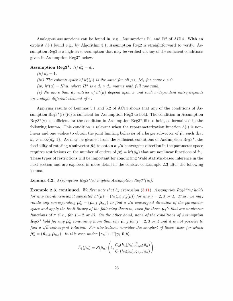
Example 2.3, continued. We first note that by expression (3.11), Assumption Reg3*(v) holds

for any two-dimensional subvector hs(µ) = (h1(µ), hj(µ)) for any j = 2, 3 or 4. Thus, we may

rotate any corresponding µsn = (µn,1, µn,j) to find a√n-convergent direction of the parameter

space and apply the limit theory of the following theorem, even for those µj’s that are nonlinear

functions of π (i.e., for j = 2 or 3). On the other hand, none of the conditions of Assumption

Reg3* hold for any µsn containing more than one µn,j for j = 2, 3 or 4 and it is not possible to

find a√n-convergent rotation. For illustration, consider the simplest of these cases for which

µsn = (µn,3, µn,4). In this case under γn ∈ Γ(γ0, 0, b),

A1(µn) = S(µn)

(1,C3(h3(µn), ζ1,n; πn)

C1(h3(µn), ζ1,n; πn)

),

25

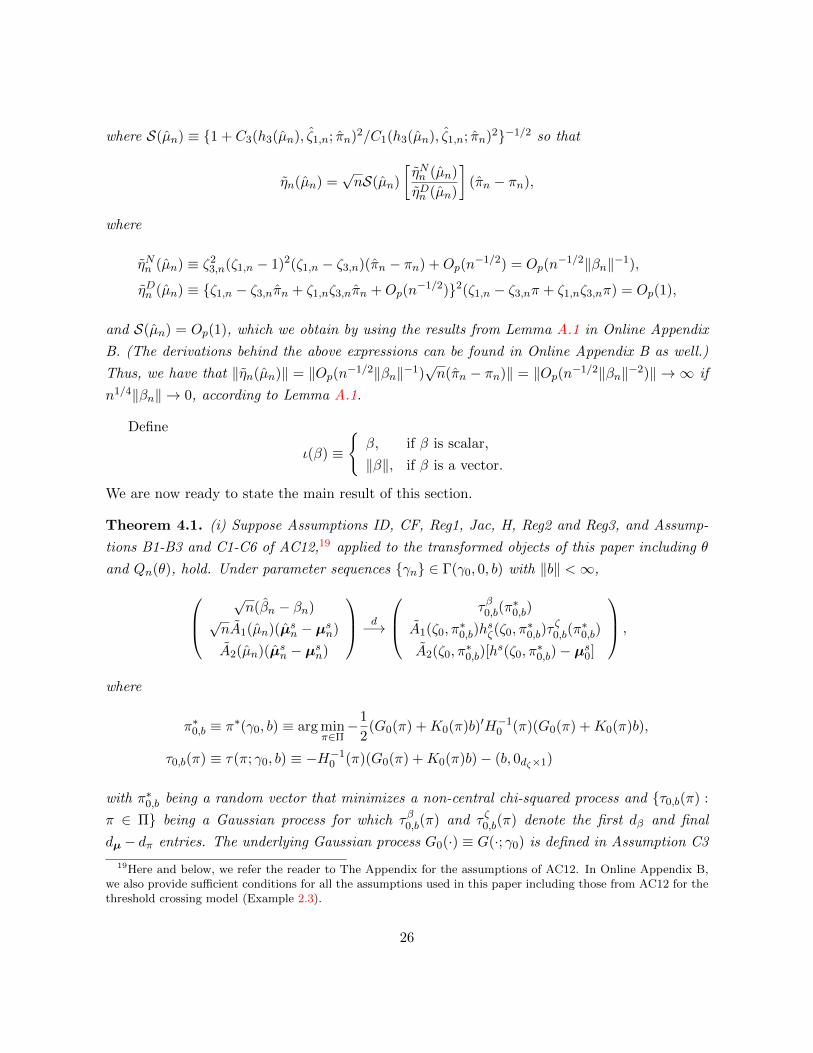
where S(µn) ≡ 1 + C3(h3(µn), ζ1,n; πn)2/C1(h3(µn), ζ1,n; πn)2−1/2 so that

ηn(µn) =√nS(µn)

[ηNn (µn)

ηDn (µn)

](πn − πn),

where

ηNn (µn) ≡ ζ23,n(ζ1,n − 1)2(ζ1,n − ζ3,n)(πn − πn) +Op(n

−1/2) = Op(n−1/2‖βn‖−1),

ηDn (µn) ≡ ζ1,n − ζ3,nπn + ζ1,nζ3,nπn +Op(n−1/2)2(ζ1,n − ζ3,nπ + ζ1,nζ3,nπ) = Op(1),

and S(µn) = Op(1), which we obtain by using the results from Lemma A.1 in Online Appendix

B. (The derivations behind the above expressions can be found in Online Appendix B as well.)

Thus, we have that ‖ηn(µn)‖ = ‖Op(n−1/2‖βn‖−1)√n(πn − πn)‖ = ‖Op(n−1/2‖βn‖−2)‖ → ∞ if

n1/4‖βn‖ → 0, according to Lemma A.1.

Define

ι(β) ≡

β, if β is scalar,

‖β‖, if β is a vector.

We are now ready to state the main result of this section.

Theorem 4.1. (i) Suppose Assumptions ID, CF, Reg1, Jac, H, Reg2 and Reg3, and Assump-

tions B1-B3 and C1-C6 of AC12,19 applied to the transformed objects of this paper including θ

and Qn(θ), hold. Under parameter sequences γn ∈ Γ(γ0, 0, b) with ‖b‖ <∞,√n(βn − βn)

√nA1(µn)(µsn − µsn)

A2(µn)(µsn − µsn)

d−→

τβ0,b(π∗0,b)

A1(ζ0, π∗0,b)h

sζ(ζ0, π

∗0,b)τ

ζ0,b(π

∗0,b)

A2(ζ0, π∗0,b)[h

s(ζ0, π∗0,b)− µs0]

,

where

π∗0,b ≡ π∗(γ0, b) ≡ arg minπ∈Π−1

2(G0(π) +K0(π)b)′H−1

0 (π)(G0(π) +K0(π)b),

τ0,b(π) ≡ τ(π; γ0, b) ≡ −H−10 (π)(G0(π) +K0(π)b)− (b, 0dζ×1)

with π∗0,b being a random vector that minimizes a non-central chi-squared process and τ0,b(π) :

π ∈ Π being a Gaussian process for which τβ0,b(π) and τ ζ0,b(π) denote the first dβ and final

dµ − dπ entries. The underlying Gaussian process G0(·) ≡ G(·; γ0) is defined in Assumption C3

19Here and below, we refer the reader to The Appendix for the assumptions of AC12. In Online Appendix B,we also provide sufficient conditions for all the assumptions used in this paper including those from AC12 for thethreshold crossing model (Example 2.3).

26

of AC12 and the underlying functions H0(π) ≡ H(π; γ0) and K0(π) ≡ K(π; γ0) are defined in

Assumptions C4(i) and C5(ii) of AC12, respectively.

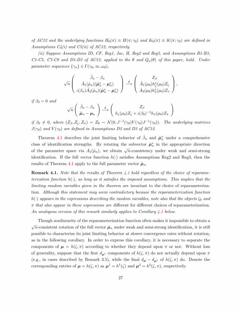
(ii) Suppose Assumptions ID, CF, Reg1, Jac, H, Reg2 and Reg3, and Assumptions B1-B3,

C1-C5, C7-C8 and D1-D3 of AC12, applied to the θ and Qn(θ) of this paper, hold. Under

parameter sequences γn ∈ Γ(γ0,∞, ω0),

√n

βn − βnA1(µn)(µsn − µsn)

ι(βn)A2(µn)(µsn − µsn)

d−→

Zβ

A1(µ0)hsζ(µ0)Zζ

A2(µ0)hsπ(µ0)Zπ

,

if β0 = 0 and

√n

(βn − βnµn − µn

)d−→

(Zβ

hζ(µ0)Zζ + ι(β0)−1hπ(µ0)Zπ

)if β0 6= 0, where (Zβ, Zζ , Zπ) = Zθ ∼ N (0, J−1(γ0)V (γ0)J−1(γ0)). The underlying matrices

J(γ0) and V (γ0) are defined in Assumptions D2 and D3 of AC12.

Theorem 4.1 describes the joint limiting behavior of βn and µsn under a comprehensive

class of identification strengths. By rotating the subvector µsn in the appropriate direction

of the parameter space via A1(µn), we obtain√n-consistency under weak and semi-strong

identification. If the full vector function h(·) satisfies Assumptions Reg2 and Reg3, then the

results of Theorem 4.1 apply to the full parameter vector µn.

Remark 4.1. Note that the results of Theorem 4.1 hold regardless of the choice of reparame-

terization function h(·), as long as it satisfies the imposed assumptions. This implies that the

limiting random variables given in the theorem are invariant to the choice of reparameteriza-

tion. Although this statement may seem contradictory because the reparameterization function

h(·) appears in the expressions describing the random variables, note also that the objects ζ0 and

π that also appear in these expressions are different for different choices of reparameterization.

An analogous version of this remark similarly applies to Corollary 4.1 below.

Though nonlinearity of the reparameterization function often makes it impossible to obtain a√n-consistent rotation of the full vector µn under weak and semi-strong identification, it is still

possible to characterize its joint limiting behavior at slower convergence rates without rotation,

as in the following corollary. In order to express this corollary, it is necessary to separate the

components of µ = h(ζ, π) according to whether they depend upon π or not. Without loss

of generality, suppose that the first dµ1 components of h(ζ, π) do not actually depend upon π

(e.g., in cases described by Remark 3.5), while the final dµ − dµ1 of h(ζ, π) do. Denote the

corresponding entries of µ = h(ζ, π) as µ1 = h1(ζ) and µ2 = h2(ζ, π), respectively.

27

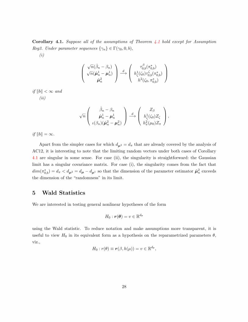
Corollary 4.1. Suppose all of the assumptions of Theorem 4.1 hold except for Assumption

Reg3. Under parameter sequences γn ∈ Γ(γ0, 0, b),

(i) √n(βn − βn)√n(µ1

n − µ1n)

µ2n

d−→

τβ0,b(π∗0,b)

h1ζ(ζ0)τ ζ0,b(π

∗0,b)

h2(ζ0, π∗0,b)

if ‖b‖ <∞ and

(ii)

√n

βn − βnµ1n − µ1

n

ι(βn)(µ2n − µ2

n)

d−→

Zβ

h1ζ(ζ0)Zζ

h2π(µ0)Zπ

,

if ‖b‖ =∞.

Apart from the simpler cases for which dµ2 = dπ that are already covered by the analysis of

AC12, it is interesting to note that the limiting random vectors under both cases of Corollary

4.1 are singular in some sense. For case (ii), the singularity is straightforward: the Gaussian

limit has a singular covariance matrix. For case (i), the singularity comes from the fact that

dim(π∗0,b) = dπ < dµ2 = dµ − dµ1 so that the dimension of the parameter estimator µ2n exceeds

the dimension of the “randomness” in its limit.

5 Wald Statistics

We are interested in testing general nonlinear hypotheses of the form

H0 : r(θ) = v ∈ Rdr

using the Wald statistic. To reduce notation and make assumptions more transparent, it is

useful to view H0 in its equivalent form as a hypothesis on the reparametrized parameters θ,

viz.,

H0 : r(θ) ≡ r(β, h(µ)) = v ∈ Rdr ,

28

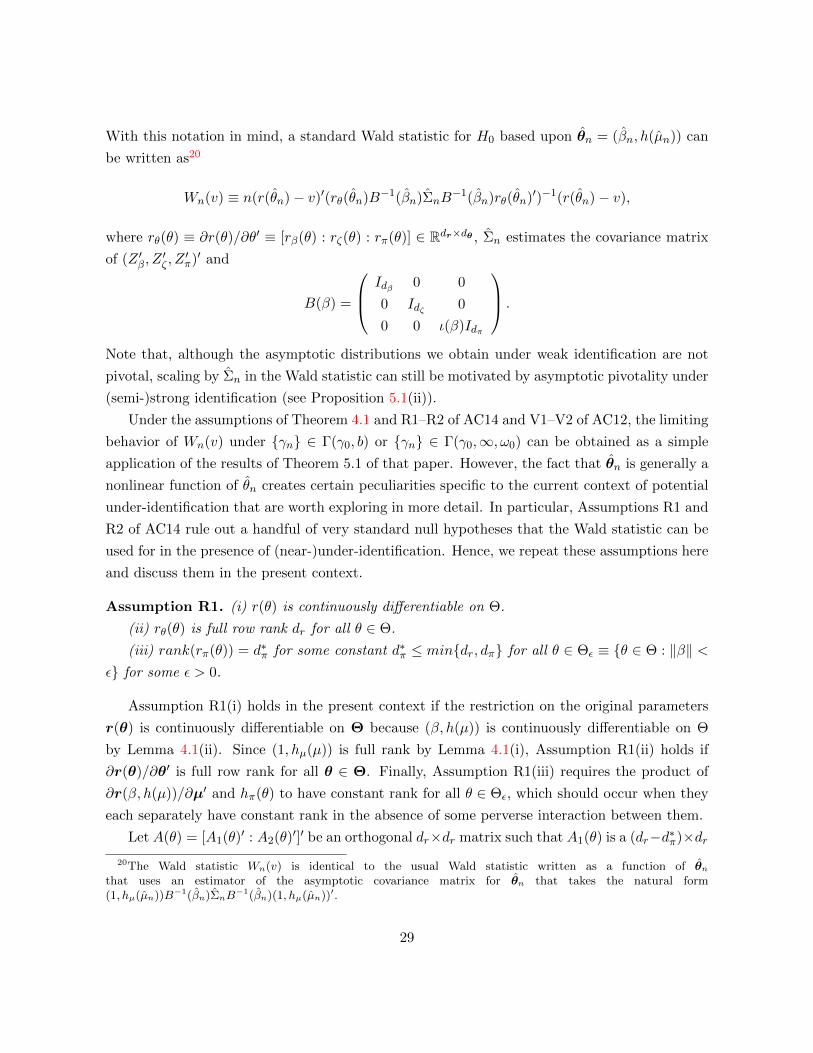
With this notation in mind, a standard Wald statistic for H0 based upon θn = (βn, h(µn)) can

be written as20

Wn(v) ≡ n(r(θn)− v)′(rθ(θn)B−1(βn)ΣnB−1(βn)rθ(θn)′)−1(r(θn)− v),

where rθ(θ) ≡ ∂r(θ)/∂θ′ ≡ [rβ(θ) : rζ(θ) : rπ(θ)] ∈ Rdr×dθ , Σn estimates the covariance matrix

of (Z ′β, Z′ζ , Z

′π)′ and

B(β) =

Idβ 0 0

0 Idζ 0

0 0 ι(β)Idπ

.

Note that, although the asymptotic distributions we obtain under weak identification are not

pivotal, scaling by Σn in the Wald statistic can still be motivated by asymptotic pivotality under

(semi-)strong identification (see Proposition 5.1(ii)).

Under the assumptions of Theorem 4.1 and R1–R2 of AC14 and V1–V2 of AC12, the limiting

behavior of Wn(v) under γn ∈ Γ(γ0, b) or γn ∈ Γ(γ0,∞, ω0) can be obtained as a simple

application of the results of Theorem 5.1 of that paper. However, the fact that θn is generally a

nonlinear function of θn creates certain peculiarities specific to the current context of potential

under-identification that are worth exploring in more detail. In particular, Assumptions R1 and

R2 of AC14 rule out a handful of very standard null hypotheses that the Wald statistic can be

used for in the presence of (near-)under-identification. Hence, we repeat these assumptions here

and discuss them in the present context.

Assumption R1. (i) r(θ) is continuously differentiable on Θ.

(ii) rθ(θ) is full row rank dr for all θ ∈ Θ.

(iii) rank(rπ(θ)) = d∗π for some constant d∗π ≤ mindr, dπ for all θ ∈ Θε ≡ θ ∈ Θ : ‖β‖ <ε for some ε > 0.

Assumption R1(i) holds in the present context if the restriction on the original parameters

r(θ) is continuously differentiable on Θ because (β, h(µ)) is continuously differentiable on Θ

by Lemma 4.1(ii). Since (1, hµ(µ)) is full rank by Lemma 4.1(i), Assumption R1(ii) holds if

∂r(θ)/∂θ′ is full row rank for all θ ∈ Θ. Finally, Assumption R1(iii) requires the product of

∂r(β, h(µ))/∂µ′ and hπ(θ) to have constant rank for all θ ∈ Θε, which should occur when they

each separately have constant rank in the absence of some perverse interaction between them.

Let A(θ) = [A1(θ)′ : A2(θ)′]′ be an orthogonal dr×dr matrix such that A1(θ) is a (dr−d∗π)×dr20The Wald statistic Wn(v) is identical to the usual Wald statistic written as a function of θn

that uses an estimator of the asymptotic covariance matrix for θn that takes the natural form(1, hµ(µn))B−1(βn)ΣnB

−1(βn)(1, hµ(µn))′.

29

matrix whose rows span the null space of rπ(θ)′ and A2(θ) is a d∗π × dr matrix whose rows span

the column space of rπ(θ). Let

ηn(θ) ≡

n1/2A1(θ) r(βn, ζn, π)− r(βn, ζn, πn) , if d∗π < dr

0, if d∗π = dr.

Assumption R2. Under γn ∈ Γ(γ0, 0, b), ηn(θn)p−→ 0 for all b ∈ Rdβ∞ .

In leading cases of interest, subvector null hypotheses, i.e., H0 : θs = v for some subvector

θs of θ, Assumption R2 is equivalent to Assumption Reg3 introduced in the previous section.21

Recalling that Assumption Reg3 is used to show a√n-convergent rotation of θsn can be con-

structed, we note that the existence of such a√n-convergent rotation is crucial to obtaining the

convergence of a subvector Wald statistic under weak and semi-strong identification sequences.

In the potential presence of the more complicated forms of identification failure we are interested

in here, standard Wald statistics for testing seemingly straightforward (linear) hypotheses can

easily diverge under the null hypothesis and weak or semi-strong identification sequences.

Remark 5.1. In cases for which ‖ηn(θn)‖ diverges, Theorem 5.2 of AC14 tells us that Wn(v)

also diverges. This is particularly important in the context of the nonlinear reparameterizations

of this paper. For example, it implies that if the reparameterization function h(·) is nonlinear,

a standard subvector Wald statistic can easily diverge when the subvector under test is “large

enough”, containing more than dπ entries of µ that are nonlinear functions of π. See the

continuation of Example 2.3 in the previous section for an example. This result is very important

in practice. It implies that subvector Wald tests making use of χ2dr

CVs exhibit size distortion

of the most extreme kind: their asymptotic size is equal to one if the subvector is large enough

(including the full vector θ).

Any one of the following sufficient conditions implies the high-level Assumption R2, as veri-

fied in Lemma 5.1 of AC14.

Assumption R2*. (i) d∗π = dr.

(ii) dr = 1.

(iii) The column space of rπ(θ) is the same for all θ ∈ Θε for some ε > 0.

In our context, Assumption R2*(i) requires the number of restrictions under test not exceed

dπ and that all restrictions must involve elements of µ that are nontrivial functions of π. In the

21This statement holds because if any elements of r(θ) are equal to elements of β, the corresponding elementsof r(βn, ζn, π)− r(βn, ζn, πn) are simply equal to zero.

30

case of subvector hypotheses, Assumption R2*(i)-(iii) is identical to Assumption Reg3*(i)-(iii)

and Assumptions Reg3*(iv) and (v) each implies Assumption R2*(iii).22

Assumption RL. r(θ) = Rθ, where R is a dr × dθ matrix with full row rank.

In the present context, Assumption RL essentially requires both the reparameterization

function h(·) and the restrictions under test to be linear, viz., h(θ) = Hθ and r(θ) = Rθ so

that r(θ) = RHθ. The reparameterization function h(·) is not generally linear. However, it is

sometimes possible to obtain linear reparameterizations in special cases for which the underlying

model is linear. See Remark 3.3. In linear models for which h(θ) = Hθ, the Wald statistic for

linear restrictions does not diverge under weak or semi-strong identification. The potential for

Wald statistic divergence for linear (including subvector) restrictions under weak or semi-strong

identification, as discussed in Remark 5.1, is truly a consequence of the nonlinearity of the

models we study in this paper.

Under a sequence γn, we consider the sequence of null hypotheses H0 : r(θ) = vn, where

vn = r(θn). In combination with our reparameterization results, direct application of Theorem

5.1 of AC14 yields the following results.

Proposition 5.1. (i) Suppose Assumptions CF, ID, Reg1, Jac, H, R1 and R2, and Assumptions

B1-B3, C1-C6 and V1 of AC12, applied to the θ and Qn(θ) of this paper, hold. Under γn ∈Γ(γ0, 0, b) with ‖b‖ <∞,

Wn(vn)d−→ λ(π∗0,b; γ0, b),

where λ(π; γ0, b) : π ∈ Π is a stochastic process defined in The Appendix.

(ii) Suppose Assumptions CF, ID, Reg1, Jac, H, R1 and R2, and Assumptions B1-B3, C1-

C5, C7-C8, D1-D3 and V2 of AC12, applied to the θ and Qn(θ) of this paper, hold. Under

γn ∈ Γ(γ0,∞, ω0),

Wn(vn)d−→ χ2

dr .

Remark 5.2. For some hypotheses, one may use the Wald statistic and robust CVs described

in the following section to conduct tests that uniformly control asymptotic size in the potential

presence of general identification failure. To better fit this result into the current literature

on hypothesis testing that is robust to general forms of identification failure, we remark here

on three leading categories of hypotheses that are of typical interest in applied work: (i) one-

dimensional hypotheses, (ii) subvector hypotheses and (iii) full vector hypotheses. Our results

are the first we are aware of that allow one to directly conduct one-dimensional hypothesis tests

for general moment condition or likelihood models that fall into the framework of this paper.

22These statements hold because β is not a function of π.

31

The methods of Andrews and Mikusheva (2016b) can only be used for these cases when the

estimation problem can be formulated in a MD framework. To use the methods of Andrews and

Guggenberger (2018) and Andrews and Mikusheva (2016a), one must rely on a power-reducing

projection or Bonferroni bound-based approach. For subvector hypotheses, our results allow one

to directly conduct hypothesis tests for a class of subvectors that are typically not “too large”

(see Example 2.3 in Section 4 and Remark 5.1). On the other hand, one may “concentrate out”

well-identified parameters to directly conduct hypothesis tests for a different class of subvectors in

moment condition models using the methods of Andrews and Guggenberger (2018) and Andrews

and Mikusheva (2016a).23 There is an interesting complementarity here between our results

and those of Andrews and Guggenberger (2018) and Andrews and Mikusheva (2016a): to use the

approach of these latter papers, the subvector must contain all parameters subject to identification

failure so that, in some sense, the subvectors cannot be “too small”. Finally, we note that except

for models that already fall under the framework of AC12, the results of our paper do not allow

one to directly conduct full vector hypotheses (due to the divergence of ηn(θn)) whereas the

methods of Andrews and Guggenberger (2018) and Andrews and Mikusheva (2016a) do. We

should also note that the frameworks of our paper and Andrews and Guggenberger (2018) or

Andrews and Mikusheva (2016a) are non-nested and a key limiting feature of our approach that

is not present in any of the other papers mentioned in this remark is that our approach applies

only to models for which a parameter governs identification strength.

Remark 5.3. We restrict focus in this paper to Wald statistics (rather than e.g., Langrange

multiplier or likelihood ratio statistics) since they do not require estimation under the null hy-

pothesis. This allows us to use the results of Section 4 and avoid restrictive assumptions on the

reparameterization function h(·) and/or the restrictions under test r(·). For example, AC12 im-

pose Assumption RQ1(iii) to analyze the likelihood ratio statistic. Though somewhat restrictive

even in their setting, such an assumption would be especially restrictive in ours since it would

typically require the separate elements of h(·) to be functions of ζ or π only, but not both at the

same time.

6 Robust Wald Inference

The limit distribution of λ(π∗0,b; γ0, b) given in Proposition 5.1(i) provides a good approximation

to the finite-sample distribution of Wn(v). This limit distribution depends upon the unknown

nuisance parameters b and γ0. Letting c1−α(b, γ0) denote the 1−α quantile of this distribution,

23Andrews and Mikusheva (2016a) cannot handle moment conditions for which the asymptotic variance matrixof the moments is singular. This occurs for the ML estimators of this paper.

32

a standard approach to CV construction for a test of size α would be to evaluate c1−α(·) at a

consistent estimate of (b, γ0). However, the nuisance parameter b and some elements in γ0 are

not consistently estimable under γn ∈ Γ(γ0, 0, b) with ‖b‖ < ∞, lending such an approach

to size distortions. This feature of the problem leads us to consider more sophisticated CV

construction methods that lead to correct asymptotic size for the test. We will restrict our focus

to testing problems for which the distribution function of λ(π∗0,b; γ0, b) in Proposition 5.1(i) only

depends upon γ0 through the parameters ζ0 and π0 and an additional consistently-estimable

finite-dimensional parameter δ0. This is the case in all of the examples we have encountered.24

Assumption FD. The distribution function of λ(π∗0,b; γ0, b) depends upon γ0 only through ζ0,

π0, and some δ0 ∈ Rdδ∞ such that under γn ∈ Γ(γ0, 0, b) or γn ∈ Γ(γ0,∞, ω0) there is an

estimator δn with δnp−→ δ0.

Given the above assumption, we may now redefine c1−α(·) to be a function of only the finite-

dimensional parameter (b, ζ0, π0, δ0). That is, let `0 = (b, ζ0, π0, δ0) and let c1−α(`0) denote the

1 − α quantile of λ(π∗0,b; γ0, b). We will “plug-in” consistent estimators for ζ0 and δ0, ζn and

δn, when constructing the CVs. The first construction is more computationally straightforward

while the second leads to tests with better finite-sample properties because it accounts for the

fact that in any finite sample, using the data to determine identification strength comes with

a positive probability of mis-categorizing the identification strength. Neglecting this fact can

induce over-rejection of the null hypothesis in finite samples.

6.1 Identification Category Selection CVs

The first type of CV we consider is the direct analog of AC12’s (plug-in and null-imposed) Type

I Robust CV. Define tn ≡ (nβ′nΣ−1ββ,nβn/dβ)1/2, where Σββ,n is equal to the upper left dβ × dβ

block of Σn and suppose κn is a sequence of constants such that κn → ∞ and κn/n1/2 → 0

(Assumption K of AC12). Then the ICS CV for a test of size α is defined as follows:

cICS1−α,n ≡

χ2dr

(1− α)−1 if tn > κn,

cLF1−α,n if tn ≤ κn

where χ2dr

(1 − α)−1 is the (1 − α) quantile of a χ2dr

-distributed random variable and cLF1−α,n ≡sup`∈Ln∩L(v) c1−α(`) with Ln ≡ ` = (b, ζ, π, δ) ∈ L : (ζ, δ) = (ζn, δn), L(v) ≡ ` ∈ L : r(θ) =

v, and L ≡ ` = (b, ζ, π, δ) ∈ Rdβ+dζ+dπ+dδ∞ : there is some γ0 ∈ Γ such that ζ = ζ0, π =

24It is possible to relax this restriction and modify the CVs accordingly. However, we have not found an examplewhere this is necessary.

33

π0, δ = δ0 and for some γn ∈ Γ(γ0), n1/2βn → b. That is, we both impose H0 and “plug-in”

consistent estimators ζn and δn of ζ0 and δ0 in the construction of the CV. This leads to tests

with smaller CVs and hence better power (see, e.g., AC12 for a discussion).25 A typical choice for

κn is κn = (log n)1/2 as it is analogous to the penalty term in the Bayesian information criterion.

Under the assumptions of Proposition 5.1, Assumption FD and the following assumption, we

can establish the correct asymptotic size of tests using the Wald statistic and ICS CVs.

Assumption DF1. The distribution function of λ(π∗0,b; γ0, b) is continuous at χ2dr

(1−α)−1 and

sup`∈L0∩L(v) c1−α(`), where L0 ≡ ` = (b, ζ, π, δ) ∈ L : (ζ, δ) = (ζ0, δ0).

This assumption is assured to hold e.g., if the distribution function of λ(π∗0,b; γ0, b) is abso-

lutely continuous. This both holds and is easy to check in most examples.

Proposition 6.1. Under the assumptions of Proposition 5.1, Assumption K of AC12 and As-

sumptions FD and DF1, lim supn→∞ supγ∈Γ:r(θ)=v Pγ(Wn(v) > cICS1−α,n) = α.

This proposition shows that for certain, namely low-dimensional, null hypotheses, a test that

rejects when the standard Wald statistic Wn(v) exceeds the ICS CV cICS1−α,n described in this

section has correct asymptotic size.

6.2 Adjusted-Bonferroni CVs

The second type of CV we consider is a modification of the adjusted-Bonferroni CV of McCloskey

(2017). The basic idea here is to use the data to narrow down the set of localization param-

eters b and parameters π from the entire space P(ζn, δn) ≡ (b, π) ∈ Rdβ+dπ∞ : for some γ0 ∈

Γ with ζ0 = ζn and δ0 = δn, π = π0 and for some γn ∈ Γ(γ0), n1/2βn → b, as in the con-

struction of least-favorable CVs, to a data-dependent set. Then one subsequently maximizes

c1−α(`) over b and π in this restricted set. Intuitively, this allows the CV to randomly adapt

to the data to determine how “guarded” we should be against potential weak identification and

which part of the parameter space Π is relevant to the finite-sample testing problem.

Let bn = n1/2βn. Using the results of Theorem 4.1, we can determine the joint asymptotic

distribution of (bn, πn) under sequences γn ∈ Γ(γ0, 0, b) with ‖b‖ < ∞, and consequently

construct an asymptotically valid confidence set for (b, π0). In the context of this paper, the

adjusted-Bonferroni CV of McCloskey (2017) uses such a confidence set for (b, π0) as the data-

dependent set to maximize c1−α(`) over. Though this may be feasible in principle, the formation

of such a confidence set would be quite computationally burdensome in our context since the

25As in AC12, one may also choose not to impose H0 in the CV construction since it is misspecified under thealternative. Then, simply replace Ln ∩ L(v) with Ln in the expression for cLF1−α. Also, any consistent estimatorsof the components of γ0 may be analogously “plugged-in”.

34

quantiles of the limit random vector (τβ0,b(π∗0,b), π

∗0,b) depend upon the underlying parameters

(b, π0) themselves.26 As a modification, here we instead propose the use of either one of two sets

as follows. For notational simplicity, we will denote either of the two sets as Ian(bn, πn), though

the second one does not depend directly on πn. The first is Ian(bn, πn) = (b, π) ∈ P(ζn, δn) :

[(bn − b)′, (πn − π)′] ˆΣ−1n [(bn − b)′, (πn − π)′]′ ≤ χ2

dβ+dπ(1− a)−1, where

ˆΣn ≡

(Σββ,n n−1/2‖βn‖−1Σβπ,n

n−1/2‖βn‖−1Σ′βπ,n n−1‖βn‖−2Σππ,n

)

with Σβπ,n denoting the upper right dβ × dπ block of Σn and Σππ,n denoting the lower right

dπ×dπ block of Σn. This set is akin to an a-level Wald confidence set for (b, π0). The second set

we propose can ease later computations: Ian(bn, πn) = (b, π) ∈ P(ζn, δn) : (bn−b)′Σ−1ββ,n(bn−b) ≤

χ2dβ

(1− a)−1. Though neither of these confidence sets has asymptotically correct coverage (at

level 1−a) under γn ∈ Γ(γ0, 0, b) with ‖b‖ <∞ sequences, they attain nearly correct coverage

as ‖b‖ → ∞. Similarly to the ICS CV in the previous subsection, one may also impose H0 and

“plug-in” the values of ζn and δn since they are consistent estimators.

Let Lan(b, γ0) = ` = (b, ζ, π, δ) ∈ Ln : (b, π) ∈ Ian(b + τβ0,b(π∗0,b), π

∗0,b) and Lan = ` =

(b, ζ, π, δ) ∈ Ln : (b, π) ∈ Ian(bn, πn). For a size-α test, the construction of the CV proceeds in

two steps:

1. Compute the smallest value ς = ς(ζn, δn,ˆΣn) such that

sup

(b,γ0)∈Rdβ∞ ×Γ:(b,ζ0,π0,δ0)∈Ln∩L(v)

P

(λ(π∗0,b; γ0, b) ≥ sup

`∈Lan(b,γ0)∩L(v)

c1−α(`) + ς

)≤ α.

2. Construct the quantity cAB1−α,n = sup`∈Lan∩L(v) c1−α(`) + ς(ζn, δn,ˆΣn). This is the adjusted-

Bonferroni CV.

By Assumption FD, the computations in Step 1 can be achieved by simulating from the joint dis-

tribution of λ(π∗0,b; γ0, b), τβ0,b(π

∗0,b) and π∗0,b over a grid of (b, γ0) values such that (b, ζ0, π0, δ0) ∈

Ln ∩ L(v) or by using more computationally efficient global optimization methods such as re-

sponse surface analysis (see e.g., Jones et al., 1998 and Jones, 2001). See Algorithm Bonf-Adj in

McCloskey (2017) for additional details on the computation of this CV. Under the assumptions

of Proposition 5.1, Assumption FD and the following assumption, we can establish the correct

asymptotic size of tests using the Wald statistic and adjusted-Bonferroni CVs.

26A similar complication arises in e.g., the formation of an asymptotically valid confidence set for the localizationparameter in a local-to-unit root autoregressive model.

35

Let La0(b, γ0) = ` = (b, ζ, π, δ) ∈ L0 : (b, π) ∈ Ia0 (b + τβ0,b(π∗0,b), π

∗0,b). When using the first

Ian(bn, πn) described above,

Ia0 (b+ τβ0,b(π∗0,b), π

∗0,b) = (b, π) ∈ P(ζ0, δ0) :

[(τβ0,b(π∗0,b)′, (π∗0,b − π)′]Σ−1

0 (b+ τβ0,b(π∗0,b), θ

∗0,b)[(τ

β0,b(π

∗0,b)′, (π∗0,b − π)′]′ ≤ χ2

dβ+dπ(1− a)−1

with

Σ0(b+ τβ0,b(π∗0,b), θ

∗0,b) ≡

(Σββ,0(θ∗0,b) ‖b+ τβ0,b(π

∗0,b)‖−1Σβπ,0(θ∗0,b)

‖b+ τβ0,b(π∗0,b)‖−1Σβπ,0(θ∗0,b)

′ ‖b+ τβ0,b(π∗0,b)‖−2Σππ,0(θ∗0,b)

)

and Σββ,0(θ∗0,b) denoting the upper left dβ × dβ block of Σ0(θ∗0,b), Σβπ,0(θ∗0,b) denoting the upper

right dβ×dπ block of Σ0(θ∗0,b), and Σππ,0(θ∗0,b) denoting the lower right dπ×dπ block of Σ0(θ∗0,b).

(The function Σ0(·) is defined in Assumption V1 of AC12.) When using the second Ian(bn, πn)

described above,

Ia0 (b+ τβ0,b(π∗0,b), π

∗0,b) = (b, π) ∈ P(ζ0, δ0) : τβ0,b(π

∗0,b)′Σ−1ββ,0(θ∗0,b)τ

β0,b(π

∗0,b) ≤ χ2

dβ(1− a)−1.

Assumption DF2. There exists some (b∗, γ∗0) ∈ Rdβ∞ × Γ such that for some γn ∈ Γ(γ∗0),

n1/2βn → b∗ and

(i) P (λ(π∗0,b∗ ; γ∗0 , b∗) ≥ sup`∈La0(b∗,γ∗0 )∩L(v) c1−α(`) + ς(ζ∗0 , δ

∗0 , Σ(b∗, γ∗0))) = α,

(ii) P (λ(π∗0,b∗ ; γ∗0 , b∗) = sup`∈La0(b∗,γ∗0 )∩L(v) c1−α(`) + ς(ζ∗0 , δ

∗0 , Σ(b∗, γ∗0))) = 0.

This assumption is a similar distributional continuity condition to Assumption DF1 that

holds in most examples.

Proposition 6.2. Under the assumptions of Proposition 5.1 and Assumptions FD and DF2,

lim supn→∞ supγ∈Γ:r(θ)=v Pγ(Wn(v) > cAB1−α,n) = α.

Similarly to Proposition 6.1, this proposition shows that for certain null hypotheses of in-

terest, a test that rejects when the Wald statistic Wn(v) exceeds the adjusted-Bonferroni CV

cAB1−α,n, whose construction is detailed in this section, has correct asymptotic size.

Remark 6.1. In combination with the standard Wald statistic, the two CV construction meth-

ods detailed in this section allow one to conduct subvector inference for subvectors of the model

parameters θ. One of the main alternative approaches to subvector inference with proven asymp-

totic size control would be to use an existing identification-robust test for the entire parameter

vector θ, such as those advanced by Andrews and Guggenberger (2018) and Andrews and Miku-

sheva (2016a), and “project the test” onto the space generated by the lower-dimensional null

36

hypothesis. Apart from their well-known poor power properties when the dimension of the full

parameter vector is substantially larger than the subvector under test, projection-based tests can

also be computationally costly. The computation of a projection-based typically involves min-

imizing a nonlinear test statistic function over the space of nuisance parameters that are not

under test. Our CV constructions also require the optimization of a nonlinear function c1−α(`)

but the dimension of the space over which the optimization is performed is equal to dβ + dπ,

which is typically of lower dimension than the nuisance parameters, at least for low-dimensional

hypotheses. Nevertheless, c1−α(`) must typically be computed via Monte Carlo simulation. So

there is no general rule for which of the two tests is easier to compute.

7 Threshold-Crossing Model Example

To illustrate our approach, we examine the threshold crossing model of a triangular system

(Example 2.3) in this section. Weak identification and robust inference have been extensively

studied in the literature (e.g., Staiger and Stock, 1997; Kleibergen, 2002; Moreira, 2003) for linear

models of a triangular system (i.e, linear IV models), but not in this nonlinear setting. The

latter, however, is empirically relevant when the dependent variable and/or endogenous regressor

are/is binary (e.g., Evans and Schwab, 1995; Goldman et al., 2001; Lochner and Moretti, 2004;

Altonji et al., 2005; Rhine et al., 2006) and instruments are potentially weak. This section

contains some of the objects that appear in the general results of this paper, applied to the

threshold crossing model. The full verification of the assumptions imposed in the theoretical

results of this paper and other technical details are contained in Online Appendix B.

The random sample is given by the vector Wi ≡ (Yi, Di, Zi) for i = 1, . . . , n. The ML

estimator θn minimizes the following criterion function in θ = (β, ζ,π1,π2, π) over the parameter

space Θ ≡ θ = (β, ζ,π1,π2, π) ∈ [−0.98 − ε, 0.98 + ε] × [0.01 − ε, 0.99 + ε] × [0.01 − ε, 0.99 +

ε]× [0.01− ε, 0.99 + ε]× [−0.99− ε, 0.99 + ε] : 0.01− ε ≤ β + ζ ≤ 0.99 + ε:

Qn(θ) =1

n

n∑i=1

ρ(Wi,θ)

for ε = 0.005, where ρ(w,θ) is a function of g(θ) via ρ(w,θ) ≡ −∑

y,d,z=0,1 1ydz(w) logpyd,z(θ),

the logarithm of density function27 with 1ydz(w) ≡ 1w = (y, d, z), and the set of pyd,z(θ)’s

are defined in (2.5)–(2.6). The parameter space Θ is chosen here to be unrestrictive while still

satisfying the conditions imposed in Online Appendix B. These latter conditions are mainly

27The log density would originally be ρ(w,θ, φ) ≡∑

y,d,z=0,1

1ydz(w) logpyd,z(θ) + log φz, but the term log φz

is dropped since it does not affect the optimization problem.

37

imposed to avoid boundary issues in the estimation of θ. See Online Appendix B and AC12 for

further details.

7.1 Asymptotic Distributional Approximations for the Estimators

In this subsection, we describe the quantities composing the asymptotic distributions of the

estimators in the threshold-crossing model example under γn ∈ Γ(γ0, 0, b) with ‖b‖ < ∞found in Theorem 4.1 and Corollary 4.1. The derivations used to obtain these quantities are

given in Online Appendix B.

After the transformation, the transformed fitted probabilities pyd,z(θ) ≡ pyd,z(β, h(µ)) can

be expressed as

p11,0(θ) = ζ3,

p11,1(θ) = C(h3(ζ1, ζ3, π), ζ1 + β;π),

p10,0(θ) = ζ2, (7.1)

p10,1(θ) = h2(ζ1, ζ2, π)− C(h2(ζ1, ζ2, π), ζ1 + β;π),

p01,0(θ) = ζ1 − ζ3,

p01,1(θ) = ζ1 + β − p11,1(θ),

and

p00,0(θ) = 1− p11,0(θ)− p10,0(θ)− p01,0(θ) = 1− ζ1 − ζ2, (7.2)

p00,1(θ) = 1− p11,1(θ)− p10,1(θ)− p01,1(θ) = 1− ζ1 − β − p10,1(θ).

The first deterministic function appearing in the results of Theorem 4.1 and Corollary 4.1 is

H(π; γ0) = −∑

y,d,z=0,1

φz,0pyd,z(θ0)

Dψpyd,z(ψ0, π)Dψpyd,z(ψ0, π)′,

where φz,0 ≡ Pγ0(Zi = z), ψ ≡ (β, ζ), ψ0 ≡ (0, ζ0) and Dψpyd,z(ψ0, π) ≡ ∂pyd,z(ψ0, π)/∂ψ. The

second one is

K(π; γ0) = −∑

y,d,z=0,1

φz,0pyd,z(θ0)

∂pyd,z(θ0)

∂β0Dψpyd,z(ψ0, π).

Finally, G(·; γ0) is a mean zero Gaussian process indexed by π ∈ Π = [−0.99, 0.99] with bounded

continuous sample paths and covariance kernel for π1, π2 ∈ Π equal to

Ω(π1, π2; γ0) = SψV†((ψ0, π1), (ψ0, π2); γ0)S′ψ,

38

where Sψ ≡ [Idψ : 0dψ×1] is a selector matrix that selects the subvector ψ from θ and

V †(θ1, θ2; γ0) ≡ Eγ0

∑y,d,z=0,1

1ydz(Wi)Dθp

†yd,z(θ1)

pyd,z(θ1)

∑y,d,z=0,1

1ydz(Wi)Dθp

†yd,z(θ2)′

pyd,z(θ2)

− Eγ0

∑y,d,z=0,1

1ydz(Wi)Dθp

†yd,z(θ1)

pyd,z(θ1)

Eγ0 ∑y,d,z=0,1

1ydz(Wi)Dθp

†yd,z(θ2)′

pyd,z(θ2)

=

∑y,d,z=0,1

pyd,z(θ0)φz,0pyd,z(θ1)pyd,z(θ2)

Dθp†yd,z(θ1)p†yd,z(θ2)′

−

∑y,d,z=0,1

pyd,z(θ0)φz,0pyd,z(θ1)

Dθp†yd,z(θ1)

∑y,d,z=0,1

pyd,z(θ0)φz,0pyd,z(θ2)

Dθp†yd,z(θ2)′

with Dθp

†yd,z(θ) ≡ B

−1(β)∂pyd,z(θ)/∂θ.

We conclude this subsection with a brief simulation study illustrating how well the weak

identification asymptotic distributions for the parameter estimators approximate their finite

sample counterparts. Here we specialize the results to the model that uses the Ali-Mikhail-Haq

copula defined in (3.10). Figures 1–3 provide the simulated finite-sample density functions of

the estimators of the threshold-crossing model parameters in the top row and their asymptotic

approximations in the bottom row. For the finite-sample distributions, we examine the true pa-

rameter values β ∈ 0, 0.1, 0.2, 0.4, ζ = 0.2 and π = (0.6, 0.4, 0.4). Under γn ∈ Γ(γ0, 0, b) the

asymptotic distributional approximations use the corresponding parameter values with b =√nβ,

ζ0 = ζ and π0 = π. Since θn = (βn, µn) = (βn, h(ζn, πn)), we use the distributions of the ele-

ments of β0 + τβ0,b(π∗0,b)/√n and h(ζ0 + τ ζ0,b(π

∗0,b)/√n, π∗0,b) as our asymptotic approximations to

the finite sample distributions of the elements of βn and µn. This approximation is asymptot-

ically equivalent to using the limiting objects in Corollary 4.1(i) but performs better in finite

samples by capturing the additional “randomness” arising from the√n-consistent parameter

estimate ζn in the distribution of µn. Figures 1–3 show that (i) the distributions of the parame-

ter estimators can be highly non-Gaussian under weak/non-identification; (ii) as β grows larger,

the distributions become approximately Gaussian; and (iii) the new asymptotic distributional

approximations perform well overall, especially in contrast with usual Gaussian approximations.

7.2 Asymptotic Distributional Approximations for Wald Statistics

Similarly to the previous subsection, we now describe the additional quantities needed to obtain

the asymptotic distributions of the Wald statistics in the threshold-crossing model example.

The derivations can similarly be found in Online Appendix B.

39

Recalling the function λ is defined in The Appendix, the only new object appearing in

λ(π∗0,b; γ0, b) in Proposition 5.1 that is not a function of the specific restrictions under test r(·)or objects described in the previous subsection is the deterministic function Σ(π; γ0). For the

threshold-crossing model, this function is given by Σ(π; γ0) = V −1(ψ0, π; γ0), where

V (ψ0, π; γ0) =∑

y,d,z=0,1

φz,0pyd,z(θ0)

Dθp†yd,z(ψ0, π)Dθp

†yd,z(ψ0, π)′.

Similarly to the previous subsection, we provide a brief simulation study to illustrate how well

the random variable λ(π∗0,b; γ0, b) from Proposition 5.1, arising as the limit of the Wald statistic

under weak identification, approximates its finite-sample counterparts. Figures 4–6 provide the

simulated finite sample density functions of Wn(v) for one-dimensional null hypotheses on the

separate elements of the parameter vector θ. This type of null hypothesis is a special case of

those satisfying Assumptions R1–R2 in Section 5. We emphasize the one-dimensional subvec-

tor testing case here, since it is often of primary interest in applied work and, to the best of

our knowledge, no other studies in the literature have developed weak identification asymptotic

results for test statistics of this form. As in the previous subsection, the finite-sample density

functions for the Wald statistics are given in the top row and the densities of λ(π∗0,b; γ0, b) are

given in the bottom row. In addition, the solid black line graphs the density function of a

χ21 distribution for comparison. We look at identical true parameter values as in the previous

subsection. Figures 4–6 show similar features to the corresponding figures for the estimators

(Figures 1–3): (i) the distributions of the Wald statistics can depart significantly from the usual

asymptotic χ21 approximations in the presence of weak/non-identification; (ii) as β grows larger,

the distributions become approximately χ21; and (iii) the new asymptotic distributional approx-

imation perform very well, especially compared to the usual χ21 approximation when β is small.

One interesting additional feature to note is that, although the distributions of the parameter

estimates when β = 0.2 in Figure 3 appear highly non-Gaussian (especially for π1 and π3), the

corresponding distributions in Figure 6 look well-approximated by the χ21 distribution. This is

perhaps due to the self-normalizing nature of Wald statistics.

7.3 Power Performance for One-Dimensional Robust Wald Tests

In this subsection, we provide a brief analysis of the power of one of our proposed robust

Wald tests when applied to the one-dimensional parameter π2 of the threshold crossing model.

Since the current literature does not contain tests with proven uniform size control for directly

testing one-dimensional hypotheses in the maximum likelihood setting, we can only compare

the power of our robust Wald test to a projected version of a full vector test. And since this

40

model is estimated by maximum likelihood, the only test we could find in the literature for the

full parameter vector θ with proven asymptotic size control is the singularity-robust Anderson

Rubin (SR-AR) test of Andrews and Guggenberger (2018) that uses the score function of the

log-likelihood as the moment function. Thus, as a baseline performance measure, we compare

the power of our robust test to the projected version of the SR-AR test.28

For testing the null hypothesis, H0 : π2 = 0.4 at the α = 0.05 level, we examine the power of

the robust Wald test that uses the (modified and) adjusted-Bonferroni CV described in Section

6.2, where we implement the CV with the second Ian(bn, πn) set described there with a = 0.5 . We

examine power under both weak and strong identification, corresponding here to β = 0.2 and 0.4.

For these two values of β, the finite sample distributions of the data are generated identically

to those in Sections 7.2-7.3 except that in order to produce power curves, we vary the true

underlying value of π2 across a space of alternative hypotheses. These power curves, along with

those of the projected SR-AR test are shown in Figure 7. Here, we can see the clear dominance

of the robust Wald test in comparison to projected SR-AR under strong identification. Under

weak identification, though the robust Wald test does not dominate, it exhibits higher power

over most of the alternative space, with especially pronounced power differences occurring at

more local alternatives.

8 Empirical Application: The Effect of Education on Crime

We now provide an identification-robust empirical analysis that revisits some of the analysis of

Lochner and Moretti (2004) on how educational attainment affects an individual’s subsequent

participation in crime. Lochner and Moretti (2004) study whether increasing one’s education

level tends to reduce their engagement in criminal behavior and whether a policy aimed at

doing so would be cost-effective relative to other crime prevention policies. These questions

relate to measuring the social returns to education that incorporate spill-over effects or exter-

nalities. As part of their analysis, Lochner and Moretti (2004) measure the effect of schooling

on incarceration using Census data. Since schooling is likely to be correlated with some of the

non-measurable factors that determine incarceration, they use differences in state compulsory

attendance laws to instrument for endogenous schooling. They find that schooling significantly

reduces the probability of incarceration. For this application, we use the same US Census data

(Lochner and Moretti’s, 2004 “inmates” data). All data and descriptions thereof are freely

available on Enrico Moretti’s website (http://eml.berkeley.edu//∼moretti/).

Of the many sets of variables examined by these authors, one fits particularly neatly into the

28Specifically, we minimize the SR-AR statistic over the remaining nuisance parameters β, ζ, π1 and π3 andcompare it to χ2

5(0.95)−1.

41

following threshold crossing model of a triangular system (Example 2.3) we examine in detail in

this paper:

Yi = 1[π1 + π2Di − εi ≥ 0]

Di = 1[ζ + βZi − νi ≥ 0], (εi, νi)

′ ∼ C(εi, vi;π3),

where C(ε, v;π3) = εv/[1 − π3(1 − ε)(1 − v)] denotes the Ali-Mikhail-Haq copula. In terms of

the variables of this model, Yi is an indicator variable that equals one if the individual is in

prison (labeled “prison” in the authors’ dataset), Di is an indicator variable that equals one if

the individual is a high school dropout (labeled “drop”) and Zi is an indicator variable that

equals one if the individual’s high school required at least 11 years of schooling (labeled “ca11”).

In this model, π2 ≡ π1 + π2 captures the counterfactual probability that an individual would

be incarcerated had they dropped out of high school, π1 is the counterfactual probability that

an individual would be incarcerated had they not dropped out, β measures how compulsory

schooling laws affect the decision to drop out from high school, ζ is equal to the probability of

dropping out for an individual attending a school without a compulsory schooling law and π3

measures the dependence between the unobserved components driving the high school drop out

decision and whether an individual becomes incarcerated.

A weak identification problem arises in the context of this application when the compul-

sory schooling laws have little (or no) effect on whether students drop out from high school,

relative to the variability of the underlying data. The weakness of compulsory schooling laws

as IVs for educational attainment decisions has been widely documented in previous literature

(e.g., Staiger and Stock, 1997). When weak identification is present in this model, the usual

large sample normal and chi-squared distributions fail to produce good approximations to the

sampling distributions of parameter estimators and Wald statistics, respectively (see Sections

7.1–7.2). This is analogous to a weak instruments problem in the standard linear IV model.

However, the non-linearity of the threshold crossing model complicates the analysis by making it

difficult to determine exactly which (functions of) parameters are weakly vs strongly identified.

This is precisely what our reparameterization method can be used to determine.

We focus on the subpopulation of black individuals as the response of black individuals

to schooling may be different than that of white individuals. Lochner and Moretti (2004) also

provide separate analyses for white vs. black individuals. We further focus on the subpopulation

of black individuals turning age 14 in 1958 or later to account both for the impact of the Supreme

Court decision Brown v. Board of Education and to mitigate cohort and/or time effects (see

Lochner and Moretti, 2004 for further details). This leaves us with a final subpopulation of

n = 184, 171 individuals.

From this subpopulation, the maximum likelihood point estimates of the threshold crossing

42

model parameters are as follows: βn = −0.0137, ζn = 0.3060, π1,n = 0.0260, π2,n = 0.0782

and π3,n = 0.0394. Loosely speaking, note that the value of βn may be indicative of weak

identification since |√nβn| = 5.879, roughly in line with b values that produce nonstandard

densities in our simulation analysis of Sections 7.1–7.2. In other words, the data indicate that

although there is evidence that the presence of a compulsory schooling law decreases the prob-

ability that a student drops out, this effect is weak enough to produce sampling distributions

for parameter estimators and test statistics that are not well-approximated by the usual nor-

mal and chi-squared approximations. The non-robust inference methods used in the original

study by Lochner and Moretti (2004) rely upon the usual large sample normal and chi-squared

approximations. In weakly identified scenarios, these types of approximations are likely to pro-

duce e.g., significance tests with actual size in exceedance of their nominal level and confidence

intervals that under-cover.

We perform robust Wald inference for the main parameter of interest π2. Rather than

comparing the Wald statistic for this parameter to the upper quantiles of a chi-squared distribu-

tion (with one degree of freedom), we approximate the null distribution by a stochastic process

evaluated at the minimizer of a non-central chi-squared process to form a confidence interval.

General expressions for these processes are given in Theorem 4.1(i) and Proposition 5.1(i). Ex-

pressions for the quantities entering these processes that are specific to the threshold-crossing

model are given in Sections 7.1–7.2. Though their expressions are involved, these processes and

the resulting distributional approximations are straightforward to simulate. By using this more

accurate nonstandard approximation to the null distribution of the Wald statistic, we produce a

confidence interval with true coverage much closer to the nominal level than would obtain under

the usual chi-squared distributional approximation.

Though they are straightforward to compute via simulation, the upper quantiles of the

nonstandard distributional approximations depend upon nuisance parameters φ1, β, ζ, b and π.

To implement our robust inference procedures, we must determine the values of these nuisance

parameters at which to simulate the distributions. The nuisance parameters φ1 = P (Zi = 1),

β and ζ = (ζ,π1 − C(π1, ζ;π3), C(π2, ζ;π3)) are consistently estimable via ML estimation

and we evaluate the nonstandard distributions at consistent estimates for these parameters.

On the other hand, the nuisance parameters b and π are not consistently estimable. For these

parameters, we compute the 0.5-level confidence set I0.5n = b ∈ R : (

√nβn−b)′Σ−1

ββ,n(√nβn−b) ≤

χ21(0.5)−1×R, where Σββ,n is

√n times the usual standard error for the ML estimator βn and

χ21(0.5)−1 is the 50th percentile of a chi-squared distribution with one degree of freedom. This

set provides us with the range of identification-strength parameters b that the data indicate

as the most relevant to this particular application. We find the largest 1 − α quantile of the

43

nonstandard distribution across the confidence set I0.5n . Finally, to correct for the fact that

(b, π) may not lie in the confidence set, we add a small constant to this largest quantile. This

constant is determined by jointly simulating the nonstandard null asymptotic distribution of the

Wald statistic and βn according to Steps 1. and 2. in Section 6.2. The sum of this constant and

largest quantile is equal to the identification-robust adjusted-Bonferroni CV. The robust Wald

test rejects when the standard Wald statistic exceeds this CV.

For a test of nominal size α = 0.05, the adjusted-Bonferroni CV just described is cAB1−α,n ≈11.5.29 Forming a robust confidence interval for π2, by finding all hypothesized values of π2

that are not rejected by the robust Wald test, we obtain a 95% confidence interval equal to

[lb∗, 0.326], where lb∗ > 0 is some small number that provides the lower bound on the true

parameter space for π2 (lb∗ must be strictly greater than zero to satisfy the parameter space

conditions in Online Appendix B). For comparison, the standard Wald confidence interval that

is not robust to weak identification is equal to [0.036, 0.12]. It is interesting to note that, in

contrast to the standard confidence interval, the robust confidence interval implies that we fail

to reject any small value of the counterfactual probability. That is, no matter how close lb∗ is

to zero, we cannot reject the null hypothesis H0 : π2 = lb∗.

29Due to the structure of the parameter space, the CV does not depend upon the null hypothesized value forπ2.

44

A Appendix: Assumptions in Andrews and Cheng (2012)

For the reader’s convenience, we restate the assumptions of AC12 that appear in the theorems in

Sections 4–6 of the current paper. At the end of this subsection, we also restate the expression

for the limit distribution of the Wald statistic of AC14 that is used in Sections 5–6. “With

respect to” is abbreviated as “w.r.t.”

Recall h(θ) ≡ (β, h(µ)). As noted in footnotes 15 and 18, the true parameter spaces for θ

and θ differ from the parameter spaces Θ and Θ. Specifically, let Θ∗ denote the true parameter

space for θ and Θ∗ ≡ h−1(Θ∗) denote the true parameter space for θ. Lemma 4.1(i) implies the

bijectivity of h : Θ∗ → Θ∗, since we assume that the true parameter space is contained in the

optimization parameter space (see Assumption B1 below). We assume that Θ∗ is a compact

subset of Rdθ . All statements made throughout the main text should technically be written with

Θ∗ and Θ∗ replacing Θ and Θ in the definitions of Γ and Γ.

Define Θ∗δ ≡ θ ∈ Θ∗ : ‖β‖ < δ, where Θ∗ is the true parameter space for θ.

Assumption B1 (AC12): (i) int(Θ) ⊃ Θ∗. (ii) For some δ > 0, Θ ⊃β ∈ Rdβ : ‖β‖ < δ

×

Z0 ×Π ⊃ Θ∗δ for some nonempty open set Z0 ⊂ Rdζ . (iii) Π is compact.

Assumption B2 (AC12): (i) Γ is compact and Γ = γ = (θ, φ) : θ ∈ Θ∗, φ ∈ Φ∗(θ). (ii) For

some δ > 0, γ = (β, ζ, π, φ) ∈ Γ with 0 ≤ ‖β‖ < δ implies that γ = (β, ζ, π, φ) ∈ Γ for all

β ∈ Rdβ with 0 ≤∥∥∥β∥∥∥ < δ. (iii) For δ > 0 as in (ii), ∃γ = (β, ζ, π, φ) ∈ Γ with 0 < ‖β‖ < δ.

Assumption B3: (i) For some nonstochastic real-valued functionQ(θ; γ0) on Θ×Γ, supθ∈Θ |Qn(θ)−Q(θ; γ0)| →p 0 under γn ∈ Γ(γ0) ∀γ0 ∈ Γ. (ii) When β0 = 0, for every neighborhood Ψ0(⊂Rdψ) of ψ0 = (β0, ζ0), infπ∈Π(infψ∈Ψ(π)/Ψ0

Q(ψ, π; γ0)−Q(ψ0, π; γ0)) > 0 ∀γ0 = (ψ0, π0, φ0) ∈ Γ.

(iii) When β0 6= 0, for every neighborhood Θ0(⊂ Θ) of θ0 = (β0, ζ0, π0), infθ∈Θ/Θ0Q(θ; γ0) −

Q(θ0; γ0) > 0 ∀γ0 = (θ0, φ0) ∈ Γ.

Assumption C1: Under γn = (βn, ζn, πn, φn) ∈ Γ(γ0, 0, b), for some δ > 0, ∀θ = (ψ, π) ∈Θδ = θ ∈ Θ : ‖β‖ < δ, the following statements hold: (i) The sample criterion function

Qn(ψ, π) has a quadratic expansion in ψ around ψ0,n = (0, ζn) for given π,

Qn(ψ, π) = Qn(ψ0,n, π) +DψQn(ψ0,n, π)′(ψ − ψ0,n)

+1

2(ψ − ψ0,n)′DψψQn(ψ0,n, π)(ψ − ψ0,n) +Rn(ψ, π),

whereDψQn(ψ0,n, π) ∈ Rdψ is a stochastic generalized first partial-derivative vector, andDψψQn(ψ0,n, π) ∈Rdψ×dψ is a generalized second partial-derivative matrix that is symmetric and may be stochastic

45

or nonstochastic. (ii) The remainder, Rn(ψ, π), satisfies

supψ∈Ψ(π):‖ψ−ψ0,n‖≤δn

∣∣a2n(γn)Rn(ψ, π)

∣∣(1 + ‖an(γn)(ψ − ψ0,n)‖)2

= opπ(1)

for all constants δn → 0, (iii) DζQn(θ) and DζζQn(θ) do not depend on π when β = 0, where

θ = (β, ζ, π) ∈ Θ, DζQn(θ) denotes the last dζ elements of DψQn(θ), and DζζQn(θ) is the lower

dζ × dζ block of DψψQn(θ).

Assumption C2: (i) DψQn(θ) takes the form DψQn(θ) = n−1∑n

i=1m(Wi, θ) for some function

m(Wi, θ) ∈ Rdψ ∀θ ∈ Θδ, for any true parameter γ∗ ∈ Γ. (ii) Eγ∗m(Wi, ψ∗, π) = 0 ∀π ∈ Π,

∀i ≥ 1 when the true parameter is γ∗ ∀γ∗ = (ψ∗, π∗, φ∗) ∈ Γ with β∗ = 0.

Define an empirical process Gn(π) : π ∈ Π by

Gn(π) = n−1/2n∑i=1

(m(Wi, ψ0,n, π)− Eγnm(Wi, ψ0,n, π)).

Assumption C3: Under γn ∈ Γ(γ0, 0, b), Gn(·) ⇒ G(·; γ0), where G(·; γ0) is a mean zero

Gaussian process indexed by π ∈ Π with bounded continuous sample paths and some covariance

kernel Ω(π1, π2; γ0) for π1, π2 ∈ Π.

Assumption C4: (i) Under γn ∈ Γ(γ0, 0, b), supπ∈Π ‖DψψQn(ψ0,n, π)−H(π; γ0)‖ →p 0

for some nonstochastic symmetric dψ × dψ matrix-valued function H(π; γ0) on Π × Γ that is

continuous on Π ∀γ0 ∈ Γ. (ii) λmin(H(π; γ0)) > 0 and λmax(H(π; γ0)) < ∞ ∀π ∈ Π, ∀γ0 ∈ Γ

with β0 = 0.

Define the dψ×dβ matrix of partial derivatives of the average population moment function w.r.t.

the true β value, β∗, to be

Kn(θ; γ∗) = n−1n∑i=1

∂

∂β∗′Eγ∗m(Wi, θ).

The domain of the function Kn(θ; γ∗) is Θδ × Γ0, where Γ0 = γa = (aβ, ζ, π, φ) ∈ Γ : γ =

(β, ζ, π, φ) ∈ Γ with ‖β‖ < δ and a ∈ [0, 1], and δ > 0 is as in Assumption B2(ii).

Assumption C5: (i) Kn(θ; γ∗) exists ∀(θ, γ∗) ∈ Θδ × Γ0, ∀n ≥ 1. (ii) For some nonstochastic

dψ × dβ matrix-valued function K(ψ0, π; γ0), K(ψn, π; γn)→ K(ψ0, π; γ0) uniformly over π ∈ Π

for all nonstochastic sequences ψn and γn such that γn ∈ Γ, γn → γ0 = (0, ζ0, π0, φ0) for

some γ0 ∈ Γ, (ψn, π) ∈ Θ, and ψn → ψ0 = (0, ζ0). (iii) K(ψ0, π; γ0) is continuous on Π ∀γ0 ∈ Γ

with β0 = 0.

46

Define a “weighted non-central chi-squared” process ξ(π; γ0, b) : π ∈ Π by

ξ(π; γ0, b) ≡ −1

2(G(π; γ0) +K(π; γ0)b)′H−1(π; γ0) (G(π; γ0) +K(π; γ0)b) .

Assumption C6: Each sample path of the stochastic process ξ(π; γ0, b) : π ∈ Π in some set

A(γ0, b) with Prγ0(A(γ0, b)) = 1 is minimized over Π at a unique point (which may depend on

the sample path), denoted π∗(γ0, b), ∀γ0 ∈ Γ with β0 = 0, ∀b with ‖b‖ <∞.

Define a non-stochastic function η(π; γ0, ω0) : π ∈ Π by

η(π; γ0, ω0) ≡ −1

2ω′0K(π; γ0)′H−1(π; γ0)K(π; γ0)ω0.

Assumption C7: The non-stochastic function η(π; γ0, ω0) is uniquely minimized over π ∈ Π

at π0 ∀γ0 ∈ Γ with β0 = 0.

Assumption C8: Under γn ∈ Γ(γ0, 0, b),∂∂ψ′EγnDψQn(ψ, πn)|ψ=ψn → H(π0; γ0).

Assumption D1: When the true parameters are γn ∈ Γ(γ0,∞, ω0), the following statements

hold: (i) The sample criterion function Qn(θ) has a quadratic expansion in θ around θn:

Qn(θ) = Qn(θn) +DQn(θn)′(θ − θn)

+1

2(θ − θn)D2Qn(θn)(θ − θn) +R∗n(θ),

whereDQn(θn) ∈ Rdθ is a stochastic generalized first derivative vector andD2Qn(θn) ∈ Rdθ×dθ is

a generalized second derivative matrix that is symmetric and may be stochastic or nonstochastic.

(ii) The remainder, R∗n(θ), satisfies

supθ∈Θn(δn)

|nR∗n(θ)|(1 +

∥∥n1/2B(βn)(θ − θn)∥∥)2

= op(1)

for all constants δn → 0, where Θn(δn) = θ ∈ Θ : ‖ψ − ψn‖ ≤ δn ‖βn‖ and ‖π − πn‖ ≤ δn.

Assumption D2: Under γn ∈ Γ(γ0,∞, ω0), Jn = B−1(βn)D2Qn(θn)×B−1(βn) →p J(γ0) ∈Rdθ×dθ , where J(γ0) is nonsingular and symmetric.

Assumption D3: (i) Under γn ∈ Γ(γ0,∞, ω0), n1/2B−1(βn)DQn(θn)→d G∗(γ0) ∼ N(0dθ , V (γ0))

for some symmetric dθ × dθ matrix V (γ0). (ii) V (γ0) is positive definite ∀γ0 ∈ Γ.

Let

Σ(θ; γ0) = J−1(θ; γ0)V (θ; γ0)J−1(θ; γ0),

47

Σ(π; γ0) = Σ(ψ0, π; γ0).

Assumption V1—Scalar β: (i) Jn = Jn(θn) and Vn = Vn(θn) for some (stochastic) dθ × dθmatrix-valued functions Jn(θ) and Vn(θ) on Θ that satisfy supθ∈Θ

∥∥∥Jn(θ)− J(θ; γ0)∥∥∥→p 0 and

supθ∈Θ

∥∥∥Vn(θ)− V (θ; γ0)∥∥∥→p 0 under γn ∈ Γ(γ0, 0, b) with ‖b‖ <∞. (ii) J(θ; γ0) and V (θ; γ0)

are continuous in θ on Θ ∀γ0 ∈ Γ with β0 = 0. (iii) λmin(Σ(π; γ0)) > 0 and λmax(Σ(π; γ0)) <∞∀π ∈ Π, ∀γ0 ∈ Γ with β0 = 0.

When β is a vector, we reparametrize β as (‖β‖ , ω), where ω = β/ ‖β‖ if β 6= 0 and

by definition ω = 1dβ/∥∥1dβ

∥∥ with 1dβ = (1, ..., 1) ∈ Rdβ if β = 0. Correspondingly, θ is

reparametrized as θ+ = (‖β‖ , ω, ζ, π). Let Θ+ = θ+ : θ+ = (‖β‖ , β/ ‖β‖ , ζ, π), θ ∈ Θ. Let θ+n

and θ+0 be the counterparts of θn and θ0 after reparametrization. Let J(θ+; γ0) and V (θ+; γ0)

denote some nonstochastic dθ × dθ matrix-valued functions such that J(θ+; γ0) = J(γ0) and

V (θ+; γ0) = V (γ0). Let

Σ(θ+; γ0) = J−1(θ+; γ0)V (θ+; γ0)J−1(θ+; γ0),

Σ(π, ω; γ0) = Σ(‖β0‖ , ω, ζ0, π; γ0),

and let Σββ(π, ω; γ0) denote the upper left dβ × dβ submatrix of Σ(π, ω; γ0).

Assumption V1—Vector β: (i) Jn = Jn(θ+n ) and Vn = Vn(θ+

n ) for some (stochastic) dθ × dθmatrix-valued functions Jn(θ+

n ) and Vn(θ+n ) on Θ+ that satisfy supθ+∈Θ+

∥∥∥Jn(θ+n )− J(θ+; γ0)

∥∥∥→p

0 and supθ+∈Θ+

∥∥∥Vn(θ+n )− V (θ+; γ0)

∥∥∥ →p 0 under γn ∈ Γ(γ0, 0, b) with ‖b‖ < ∞. (ii)

J(θ+; γ0) and V (θ+; γ0) are continuous in θ+ on Θ+ γ0 ∈ Γ with β0 = 0. (iii) λmin(Σ(π, ω; γ0)) >

0 and λmax(Σ(π, ω; γ0)) < ∞ ∀π ∈ Π, ∀ω ∈ Rdβ with ‖ω‖ = 1, ∀γ0 ∈ Γ with β0 = 0. (iv)

Pr[τβ(π∗(γ0, b), γ0, b) = 0] = 0 ∀γ0 ∈ Γ with β0 = 0 and ∀b with ‖b‖ <∞.

Assumption V2: Under γn ∈ Γ(0,∞, ω0), Jn →p J(γ0) and Vn →p V (γ0).

Assumption K: (i) κn →∞ and (ii) κn/n1/2 → 0.

Lastly, we restate the expression for the limit distribution of the Wald statistic. Define a

stochastic process λ(π; γ0, b) : π ∈ Π by

λ(π; γ0, b) = τA(π; γ0, b)′B(π; γ0, b)(r

∗θ(ψ0, π)Σ(π; γ0, b)r

∗θ(ψ0, π)′)−1B(π; γ0, b)τ

A(π; γ0, b),

where

τA(π; γ0, b) =

(r∗ψ(ψ0, π)τ(π; γ0, b)

A2(ψ0, π)(r(ψ0, π)− r(ψ0, π0))

)∈ Rdr ,

48

B(π; γ0, b) =

[I(dr−d∗π) 0

0 ι(τβ(π; γ0, b))Id∗π

],

Σ(π; γ0, b) =

Σ(π; γ0) if β is a scalar,

Σ(π, ω∗(π; γ0, b); γ0) if β is a vector,

ω∗(π; γ0, b) =τβ(π; γ0, b)

‖τβ(π; γ0, b)‖.

49

References

Altonji, J. G., Elder, T. E., Taber, C. R., 2005. An evaluation of instrumental variable strategies

for estimating the effects of catholic schooling. Journal of Human resources 40 (4), 791–821.

7

Andrews, D. W. K., Cheng, X., 2012. Estimation and inference with weak, semi-strong, and

strong identificationith weak, semi-strong, and strong identification. Econometrica 80, 2153–

2211. 1

Andrews, D. W. K., Cheng, X., 2013. Maximum likelihood estimation and uniform inference

with sporadic identification failure. Journal of Econometrics 173, 36–56. 1

Andrews, D. W. K., Cheng, X., 2014. GMM estimation and uniform subvector inference with

possible identification failure. Econometric Theory 30, 287–333. 1

Andrews, D. W. K., Guggenberger, P., 2018. Identification- and singularity-robust inference for

moment condition models, Cowles Foundation Discussion Paper No. 1978. 1, 2, 5.2, 6.1, 7.3

Andrews, I., Mikusheva, A., 2016a. Conditional inference with a functional nuisance parameter.

Econometrica 84, 1571–1612. 1, 2, 5.2, 23, 6.1

Andrews, I., Mikusheva, A., 2016b. A geometric approach to weakly identified econometric

models. Econometrica 84, 1249–1264. 1, 2, 5.2

Antoine, B., Renault, E., 2009. Efficient GMM with nearly-weak instruments. Econometrics

Journal 12, 135–171. 1, 4

Antoine, B., Renault, E., 2012. Efficient minimum distance estimation with multiple rates of

convergence. Journal of Econometrics 170, 350–367. 1, 4

Arellano, M., Hansen, L. P., Sentana, E., 2012. Underidentification? Journal of Econometrics

170, 256–290. 1

Choi, I., Phillips, P. C. B., 1992. Asymptotic and finite sample distribution theory for IV

estimators and tests in partially identified structural equations. Journal of Econometrics 51,

113–150. 1, 3.3, 4

Cox, G., 2018. Weak identification in a class of generically identified models with an application

to factor models, Unpublished Manuscript, Department of Economics, Columbia University.

1

50

Dovonon, P., Renault, E., 2013. Testing for common conditionally heteroskedastic factors.

Econometrica 81, 2561–2586. 1

Dunbar, G. R., Lewbel, A., Pendaku, K., 2013. Children’s resources in collective households:

Identification, estimation, and an application to child poverty in Malawi. American Economic

Review 103, 438–471. 2.4

Escanciano, J. C., Zhu, L., 2013. Set inferences and sensitivity analysis in semiparametric condi-

tionally identified models, Unpublished Manuscript, Indiana University, Department of Eco-

nomics. 1, 3

Evans, W. N., Schwab, R. M., November 1995. Finishing high school and starting college: Do

catholic schools make a difference? The Quarterly Journal of Economics 110 (4), 941–74. 7

Goldman, D., Bhattacharya, J., Mccaffrey, D., Duan, N., Leibowitz, A., Joyce, G., Morton, S.,

2001. Effect of Insurance on Mortality in an HIV-Positive Population in Care. Journal of the

American Statistical Association 96 (455). 7

Han, S., 2009. Identification and inference in a bivariate probit model with weak instruments.

Unpublished Manuscript, Department of Economics, Yale University. ∗

Han, S., Vytlacil, E., 2017. Identification in a generalization of bivariate probit models with

dummy endogenous regressors. Journal of Econometrics 199, 63–73. 2.3, 7

Heckman, J. J., 1979. Sample selection bias as a specification error. Econometrica 47, 153–161.

2.1

Heckman, J. J., Honore, B. E., 1990. The empirical content of the Roy model. Econometrica 58,

1121–1149. 2.2

Jones, D. R., 2001. A taxonomy of global optimization methods based on response surfaces.

Journal of Globabl Optimization 21, 345–383. 6.2

Jones, D. R., Schonlau, M., Welch, W. J., 1998. Efficient global optimization of expensive black-

box functions. Journal of Global Optimization 13, 455–492. 6.2

Kleibergen, F., 2002. Pivotal statistics for testing structural parameters in instrumental variables

regression. Econometrica 70, 1781–1803. 1, 7

Kleibergen, F., 2005. Testing parameters in GMM without assuming that they are identified.

Econometrica 73, 1103–1123. 1

51

Komunjer, I., Ng, S., 2011. Dynamic identification of dynamic stochastic general equilibrium

models. Econometrica 79, 1995–2032. 3.4

Lee, L. F., Chesher, A., 1986. Specification testing when score statistics are identically zero.

Journal of Econometrics 31, 121–149. 1

Lochner, L., Moretti, E., 2004. The effect of education on crime: evidence from prison inmates,

arrests, and self-reports. American Economic Review 94, 155–189. 7, 8

McCloskey, A., 2017. Bonferroni-based size-correction for nonstandard testing problems. Journal

of Econometrics 200, 17–35. 1, 6.2, 6.2

Moreira, M. J., 2003. A conditional likelihood ratio test for structural models. Econometrica 71,

1027–1048. 1, 7

Phillips, P. C. B., 1989. Partially identified econometric models. Econometric Theory 5, 181–240.

1, 3.3, 4

Phillips, P. C. B., 2016. Inference in near-singular regression. In: G. Gonzalez-Rivera, R. C. H.,

Lee, T.-H. (Eds.), Essays in Honor of Aman Ullah. Vol. 36 of Advances in Econometrics.

Emerald Group Publishing Limited, pp. 461–486. 1, 3.3, 4

Qu, Z., Tkachenko, D., 2012. Identification and frequency domain quasi-maximum likelihood es-

timation of linearized dynamic stochastic general equilibrium models. Quantitative Economics

3, 95–132. 1, 3, 3.4

Quarteroni, A., Sacco, R., Saleri, F., 2010. Numerical mathematics. Vol. 37. Springer Science &

Business Media. 3.2

Rhine, S. L., Greene, W. H., Toussaint-Comeau, M., 2006. The importance of check-cashing

businesses to the unbanked: Racial/ethnic differences. Review of Economics and Statistics

88 (1), 146–157. 7

Rothenberg, T. J., 1971. Identification in parametric models. Econometrica 39, 577–591. 1

Sargan, J. D., 1983. Identification and lack of identification. Econometrica 51, 1605–1633. 1, 4

Sims, C. A., Stock, J. H., Watson, M. W., 1990. Inference in linear time series models with some

unit roots. Econometrica 58, 113–144. 4

Staiger, D., Stock, J. H., 1997. Instrumental variables regression with weak instruments. Econo-

metrica 65, 557–586. 1, 7, 8

52

Stock, J. H., Wright, J. H., 2000. GMM with weak identification. Econometrica 68, 1055–1096.

1

Tommasi, D., Wolf, A., 2018. Estimating household resource shares: a shrinkage approach.

Economics Letters 163, 75–78. 2.4

53

Figure 1: Threshold Crossing Model Parameter Estimator Densities when b = 0

Asymptotic (bottom row) and finite-sample (top row, n = 1000) densities of the estimatorsof β, ζ, π3, π1 and π2 (left-to-right) in the Threshold-Crossing model when ζ = 0.2 andπ = (0.6, 0.4, 0.4).

Figure 2: Threshold Crossing Model Parameter Estimator Densities when b =√n0.1

Asymptotic (bottom row) and finite-sample (top row, n = 1000) densities of the estimatorsof β, ζ, π3, π1 and π2 (left-to-right) in the Threshold-Crossing model when ζ = 0.2 andπ = (0.6, 0.4, 0.4).

54

Figure 3: Threshold Crossing Model Parameter Estimator Densities when b =√n0.2

Asymptotic (bottom row) and finite-sample (top row, n = 1000) densities of the estimatorsof β, ζ, π3, π1 and π2 (left-to-right) in the Threshold-Crossing model when ζ = 0.2 andπ = (0.6, 0.4, 0.4).

Figure 4: Wald Statistic Densities for the Threshold Crossing Model when b = 0

Asymptotic (bottom row) and finite-sample (top row, n = 1000) densities of the Wald statisticfor the parameters β, ζ, π3, π1 and π2 (left-to-right) in the Threshold-Crossing model whenζ = 0.2 and π = (0.6, 0.4, 0.4), with a χ2

1 density overlay (bold line).

55

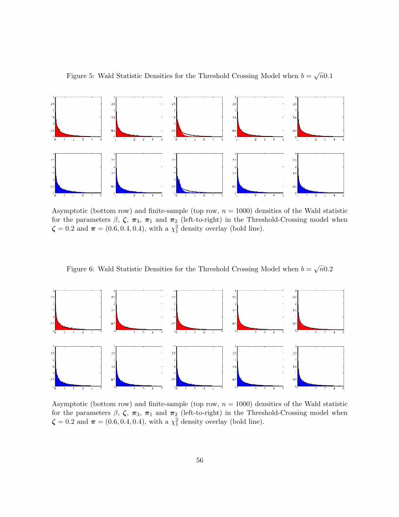
Figure 5: Wald Statistic Densities for the Threshold Crossing Model when b =√n0.1

Asymptotic (bottom row) and finite-sample (top row, n = 1000) densities of the Wald statisticfor the parameters β, ζ, π3, π1 and π2 (left-to-right) in the Threshold-Crossing model whenζ = 0.2 and π = (0.6, 0.4, 0.4), with a χ2

1 density overlay (bold line).

Figure 6: Wald Statistic Densities for the Threshold Crossing Model when b =√n0.2

Asymptotic (bottom row) and finite-sample (top row, n = 1000) densities of the Wald statisticfor the parameters β, ζ, π3, π1 and π2 (left-to-right) in the Threshold-Crossing model whenζ = 0.2 and π = (0.6, 0.4, 0.4), with a χ2

1 density overlay (bold line).

56

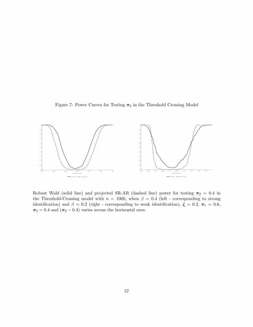
Figure 7: Power Curves for Testing π2 in the Threshold Crossing Model

0

0.1

0.2

0.3

0.4

0.5

0.6

0.7

0.8

0.9

1

-0.266 -0.171 -0.076 0.019 0.114 0.209 0.304

deviationfromnull

RobustWald ProjectedSR-AR

0

0.1

0.2

0.3

0.4

0.5

0.6

0.7

0.8

0.9

1

-0.38 -0.285 -0.19 -0.095 0 0.095 0.19 0.285 0.38 0.475

deviationfromnull

RobustWald ProjectedSR-AR

Robust Wald (solid line) and projected SR-AR (dashed line) power for testing π2 = 0.4 inthe Threshold-Crossing model with n = 1000, when β = 0.4 (left - corresponding to strongidentification) and β = 0.2 (right - corresponding to weak identification), ζ = 0.2, π1 = 0.6,π3 = 0.4 and (π2 − 0.4) varies across the horizontal axes.

57