Estimating the Natural Rates in the

New Keynesian Framework ∗

Hilde C. Bjørnland†

Norwegian School

of Management (BI)

and

Norges Bank

Kai Leitemo

Norwegian School

of Management (BI)

Junior Maih

Norges Bank

June 21, 2007

Abstract

The time-varying natural rate of interest and output and the implied medium-

term inflation target for the US economy are estimated over the period 1983-2005.

The estimation is conducted within the New-Keynesian framework using Bayesian

and Kalman-filter estimation techniques. Employing the model-consistent estimate

of the output gap, we get a small weight on the backward-looking component of the

New-Keynesian Phillips curve – similar to studies which use labor share of income

as a proxy for marginal costs (e.g., Galı et al., 2001, 2003). The turning points of the

business cycle are nevertheless broadly consistent with those of CBO/NBER. We

find considerable variation in the natural rate of interest while the inflation target

has been close to 2% over the last decade.

JEL-codes: C51, E32, E37, E52.

Keywords: Natural rate of interest, natural rate of output, New-Keynesian model,

inflation target.

∗We are grateful to Ida Wolden Bache, Leif Brubakk, Santiago Acosta Ormaechea, Scott Schuh andseminar participants at the 2006 Dynare Conference in Paris, the CEF 2007 Conference in Montreal andthe 11th ICMAIF conference in Crete 2007 for comments. We also thank John Williams for providinginformation from the updated estimation of the model in Laubach and Williams (2003). The authorsthank the Norwegian Financial Market Fund under the Norwegian Research Council for financial support.Views expressed are those of the authors and do not necessarily reflect the views of Norges Bank.

†Corresponding author: Department of Economics, Norwegian School of Management (BI), Ny-dalsveien 37, 0442 OSLO. Email: hilde.c.bjornland@bi.no.

1

1 Introduction

The New Keynesian theory as developed Goodfriend and King (1997), Rotemberg and

Woodford (1997), McCallum and Nelson (1999a) and others, and with policy implications

extensively explored in Clarida et al. (1999) and Woodford (2003), has become the leading

framework for the analysis of monetary policy. This theory honors the proposition that

monetary policy affects only nominal variables in the long run and that the steady-state

inflation rate can be governed by monetary policy. Moreover, it assumes that the central

bank implements its policy through the setting of the short-term interest rate. Monetary

policy influences decisions about real magnitudes due to prices not being fully free to

adjust to shocks (price rigidities). The overriding objective of monetary policy is to

alleviate the effects of these rigidities while keeping inflation expectations close to a target

rate of inflation.

An important point of reference for the policymaker is therefore how the economy

would have developed had prices been without rigidities and instead fully flexible. We

refer to the rate of interest and the level of output in such an equilibrium as the natural

rates of interest rates and the natural level of output (see Woodford, 2003). Consistent

with this view, the strategy of monetary policy is often formulated in terms of deviations

from these natural rates, that is, in terms of the interest rate gap and the output gap

respectively. The well-known Taylor rule (Taylor, 1993) provides an illustration. Under

the Taylor rule, the central bank raises the interest rate relative to the natural rate of

interest if either inflation deviates from the inflation target and/or output deviates from

the natural rate of output. In steady state, where there is no need for monetary policy

to respond to shocks, the interest rate equals the natural rate. For these reasons, the

natural rates are important indicators for the setting of the policy instrument and the

characterization of a neutral monetary policy stance.

2

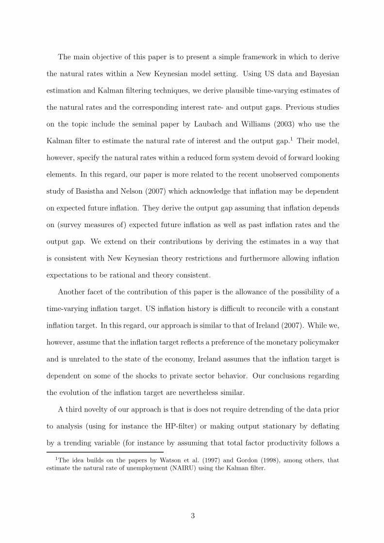
The main objective of this paper is to present a simple framework in which to derive

the natural rates within a New Keynesian model setting. Using US data and Bayesian

estimation and Kalman filtering techniques, we derive plausible time-varying estimates of

the natural rates and the corresponding interest rate- and output gaps. Previous studies

on the topic include the seminal paper by Laubach and Williams (2003) who use the

Kalman filter to estimate the natural rate of interest and the output gap.1 Their model,

however, specify the natural rates within a reduced form system devoid of forward looking

elements. In this regard, our paper is more related to the recent unobserved components

study of Basistha and Nelson (2007) which acknowledge that inflation may be dependent

on expected future inflation. They derive the output gap assuming that inflation depends

on (survey measures of) expected future inflation as well as past inflation rates and the

output gap. We extend on their contributions by deriving the estimates in a way that

is consistent with New Keynesian theory restrictions and furthermore allowing inflation

expectations to be rational and theory consistent.

Another facet of the contribution of this paper is the allowance of the possibility of a

time-varying inflation target. US inflation history is difficult to reconcile with a constant

inflation target. In this regard, our approach is similar to that of Ireland (2007). While we,

however, assume that the inflation target reflects a preference of the monetary policymaker

and is unrelated to the state of the economy, Ireland assumes that the inflation target is

dependent on some of the shocks to private sector behavior. Our conclusions regarding

the evolution of the inflation target are nevertheless similar.

A third novelty of our approach is that is does not require detrending of the data prior

to analysis (using for instance the HP-filter) or making output stationary by deflating

by a trending variable (for instance by assuming that total factor productivity follows a

1The idea builds on the papers by Watson et al. (1997) and Gordon (1998), among others, thatestimate the natural rate of unemployment (NAIRU) using the Kalman filter.

3

trend stationary process), as has been common practice in many recent DSGE analysis,

including Edge et al. (2005), Juillard et al. (2005) and Smets and Wouters (2003, 2007)

who also estimate the natural rates.2

An important empirical finding is that inflation is primarily a forward-looking process.

By allowing inflation to have both forward-looking and backward-looking components,

using a hybrid New-Keynesian Phillips curve, data prefers a forward-looking specification.

Although this is the common conclusion in studies which use labor’s share of income as

a proxy for marginal costs (see Galı et al., 2001, 2003), it is not common finding when

the output gap is the proxy. Interestingly, after accounting for the time-varying inflation

target and natural rate of interest, a model-consistent estimate of the output gap shares

some of the same properties as labor’s share of income in representing marginal costs.

This conveniently suggests that the approach of studying monetary policy within the

small and simple model framework with inflation, output gap and the interest rate, as

advocated in Woodford (2003), seems sensible.

The remainder of this paper is organized as follows. In Section 2 we present the

New Keynesian framework. Section 3 presents the estimation framework and results. In

Section 4 we provide some concluding remarks.

2 The New Keynesian Framework

The New Keynesian framework3 assumes that firms operate in monopolistic competitive

markets and production is constrained by aggregate demand. Prices are assumed to be

sticky and consequently do not move instantaneously to movements in marginal costs. Due

to the price stickiness, the central bank affects aggregate demand through its influence

2A recent exception is Juillard et al. (2006). They allow for a more general stochastic process wherethere could be both temporary changes in the growth rate of total factor productivity as well as auto-correlated deviations from steady state.

3See Goodfriend and King (1997), Rotemberg and Woodford (1997), Rotemberg and Woodford (1999),McCallum and Nelson (1999b) and Clarida et al. (1999).

4

on real interest rates. By lowering real interest rates, the central bank induces higher

aggregate demand, marginal costs and prices than would otherwise materialize. As noted

above, the natural rate of interest rate can be regarded as the neutral stance of monetary

policy - the real interest rate that produces zero output gap and stable inflation.

In estimating the natural rates, we build on the economic structure provided by the

New Keynesian framework. The basic model is extended with external habit formation

in consumption (Fuhrer, 2000) and a hybrid New-Keynesian Phillips curve that allows

for both forward-looking and backward-looking elements. This set up is rationalized by

the Calvo (1983) framework with some of the firms setting prices in accordance to an

indexation scheme (Christiano et al., 2005) or in accordance with some rule-of-thumb

(Galı and Gertler, 1999).

The approach remains nevertheless conservative regarding the extent of the economic

structure regarding production technology and the structure of the labor market imposed

in estimation. This reduces the approach’s rigor at the gain of not being tied up to a

particular description of production technology which may bias the result if incorrect.

Specifically, we allow the natural rate of output to follow exogenous processes and in this

regard, the paper draws on the literature on structural time-series estimation, see e.g.

Harvey (1989).

2.1 Aggregate demand

We assume that the economy consists of a representative household that lives forever and

maximizes expected utility given by

U = Et

∞∑

i=0

(

1

1 + δ

)i[

1

(1 − σ)

(

Ct+iVt+i

Ht+i

)(1−σ)]

,

5

subject to the intertemporal budget constraint given by

Ct +Mt

Pt

+Bt

Pt

=

(

Wt

Pt

)

Nt +Mt−1

Pt

+ It−1Bt−1

Pt

−Tt

Pt

+ Πt.

δ is the discount rate, σ is the intertemporal elasticity of substitution and C is an CES

index of consumption goods. V is a consumption preference shock. The consumer is

also assumed to have preferences over money and leisure, but for simplicity, these are not

explicitly modeled.

The consumer can either hold money (M) or bonds (B) as a store of wealth. Money

yields utility (not modeled) whereas bonds yield a gross risk-free return of It in every

period. Consumption preferences are subject to a shock Vt ≡ (1 − vt) where

vt = ρvvt−1 + vt (1)

and vt is a white-noise shock. Ht represents external habit persistence. We allow habit

persistence to be of order 2 and specify as follows

Ht = Cγ1

t−1Cγ2

t−2

where γ1 and γ2 are habit parameters. This more general setup allows agents to form

habits with respect to the changes in as well as the level of consumption.

The first-order condition for the solution to the problem implies the consumption Euler

equation

(

CtVt

Cγ1

t−1Cγ2

t−2

)1−σ1

Ct

=

(

1

1 + δ

)

ItEt

(

Ct+1Vt+1

Cγ1

t Cγ2

t−1

)1−σ1

Ct+1

Pt

Pt+1

. (2)

6

Taking the logarithm of the Euler equation and using the resource constraint, we have

yt =σ

AEtyt+1 +

(γ1 − γ2) (σ − 1)

Ayt−1 (3)

+γ2 (σ − 1)

Ayt−2 −

1

A(it −Etπt+1 − δ) +

(σ − 1)

A(vt − Etvt+1) ,

where A ≡ σ + γ1 (σ − 1) and πt is quarterly inflation at an annual rate. A small letter

denotes the log of the corresponding capital letter variable.4

Note that due to dynamic homogeneity, we can write the aggregate demand schedule

(3) as

∆yt =σ

γ1 (σ − 1)Et∆yt+1 −

γ2

γ1∆yt−1 (4)

−1

γ1 (σ − 1)(it − Etπt+1 − ρ) +

1

γ1(vt −Etvt+1) .

2.2 Aggregate supply

Aggregate supply is represented by the hybrid Phillips curve as

πt = µEtπt+1 + (1 − µ)

4∑

j=1

αjπt−j + ζmct + εt

where (1−µ) is the weight on the backward-looking component and mct is marginal costs

as of time t. As in Rudebusch (2002a,b), we allow for a lag structure on past inflation

to match the dynamics of inflation at the quarterly frequency. Furthermore, we impose

dynamic homogeneity, i.e., that α4 = 1 − α1 − α2 − α3.5 We assume that log marginal

4Note that we have for simplicity ignored Jensen’s inequality and used first-order Taylor approxima-tions, implying lnE(1 + x) = E ln(1 + x) = Ex.

5Although we do not provide any microfoundations for these lags, we postulate that these lags willfollow from the rules-of-thumb framework of pricing of Galı and Gertler (1999) given that rule-of-thumballows for longer lags.

7

costs are linear in log deviation of output from its natural rate, i.e.,

mct = γ (yt − ynt ) ,

where ynt is the natural rate of output. By defining the deviation of output from the

natural rate as the output gap, xt ≡ yt − ynt , we can write the Phillips curve as

πt = µEtπt+1 + (1 − µ)4

∑

j=1

αjπt−j + κxt + εt, (5)

where κ ≡ ζγ. The natural rate of output is given exogenously by the process

∆ynt = v + ωt (6)

where ν is the unconditional expected growth rate of output and ωt is an AR(1) shock to

the growth rate6

ωt = φωt−1 + t. (7)

The output gap follows the process

xt = xt−1 + ∆yt − ∆ynt . (8)

6The shock is best thought of as representing variations in productivity and preferences that influencethe marginal rate of substitution between consumption and leisure. Neither sources is modeled explicitlyhere.

8

2.3 Monetary policy

The monetary authority is setting the interest rate in accordance with a dynamic Taylor

rule as

it = ψit−1 + (1 − ψ)(

int + θπ

(

πt − πTt

)

+ θxxt

)

+ ut, (9)

where ψ measures the smoothing in the interest rate setting. int is the nominal natural

interest rate (defined below) and

πt ≡1

4

3∑

j=0

πt−j

is the four-quarter inflation at an annual rate. We assume that the intermediate-run

inflation target evolves according to

πTt = (1 − ρπ)π∗ + ρππ

Tt−1 + ξt, (10)

where π∗ is the steady-state inflation rate (or long-run inflation target) and ξt is an AR(1)

shock to the inflation target, following

ξt = ρκξt−1 + κt. (11)

2.4 The natural interest rate

The process for the natural nominal rate of interest can be found by replacing output and

the interest rate in equation (3) with the natural rates and then solving for the interest

9

rate, i.e.,

ynt =

σ

AEty

nt+1 +

(γ1 − γ2) (σ − 1)

Ayn

t−1 (12)

+γ2 (σ − 1)

Ayn

t−2 −1

A(int − Etπt+1 − δ) +

(σ − 1)

A(vt − Etvt+1) ,

or

∆ynt =

σ

γ1 (σ − 1)Et∆y

nt+1 −

γ2

γ1

∆ynt−1 (13)

−1

γ1 (σ − 1)(int −Etπt+1 − δ) +

1

γ1(vt − Etvt+1) .

and isolating for the natural interest rate

int = δ + Etπt+1 + σEt∆ynt+1 − γ1 (σ − 1)∆yn

t − γ2(σ − 1)∆ynt−1 (14)

+(σ − 1) (vt −Etvt+1) .

The natural real interest rate is then found from the Fisher equation as

rnt ≡ int −Etπt+1. (15)

The output gap process can be expressed as a function of the natural interest rate by

subtracting equation (12) from equation (3) which gives

xt =σ

AEtxt+1 +

(γ1 − γ2) (σ − 1)

Axt−1 (16)

+γ2 (σ − 1)

Axt−2 −

1

A(it − int )

where the natural rate of interest is given in equation (14) above.

10

3 Estimation

We estimate the parameters of the model comprising of equations (1), (4), (5), (6), (7),

(8), (9), (10) and (11) using Bayesian methods and the Kalman filter. The focus of the

analysis will be on the estimation of the natural real rate of interest and the output gap.

The use of Bayesian methods to estimate DSGE models has increased over recent years,

in a variety of contexts, see An and Schorfheide (2006) for a recent evaluation. The focus

is on methods that are built around a likelihood function, typically derived from a DSGE

model (see, e.g., Adolfson et al., 2005). With sensible priors, Bayesian techniques offer

a major advantage over other system estimators such as maximum likelihood, which in

small samples can often allow key parameters to wander off in nonsensical directions.

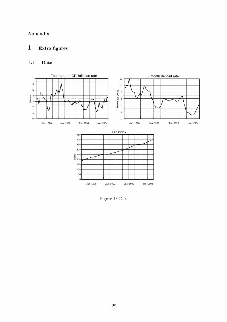
3.1 Data

We estimate the model laid out in the previous section using U.S. quarterly time series

for three variables: real output, inflation and interest rates. The sample period is 1983q1

to 2005q4. The period covers the last part of the Volcker period and the major part

of the Greenspan period. The choice of periods follows from the assumption that these

two Chairmen shares approximately the same dislike for inflation. The monetary policy

regime is therefore roughly constant over the sample period. We use the quarterly average

daily readings of US 3-month deposit rates as the relevant nominal interest rate. For real

output and inflation we use real GDP and the CPI, all items, for total USA. GDP and

CPI are seasonally adjusted by their original source (OECD). We treat inflation, output

growth, and the nominal interest rate as stationary, and express them in deviations from

their sample mean. Note that all changes are measured at an annual rate. Inflation,

output and 3-month deposit rates are plotted in Figure 1.1 in the appendix.

11

3.2 Parameter estimation

As is well known from Bayes’s rule, the posterior distribution of the parameters is pro-

portional to the product of the prior distribution of the parameters and the likelihood

function of the data. This prior distribution describes the available information prior to

observing the data used in the estimation. The observed data is then used to update the

prior, via Bayes theorem, to the posterior distribution of the model’s parameters.

To implement the Bayesian estimation method, we need to be able to evaluate nu-

merically the prior and the likelihood function. Then we use the Metropolis-Hastings

algorithm to obtain random draws from the posterior distribution, from which we obtain

the relevant moments of the posterior distribution of the parameters.

More specifically, the model is estimated in two steps in Dynare-Matlab. In the first

step we compute the posterior mode using ’csminwel’, an optimization routine developed

by Christopher Sims. We use the first three years of the full sample 1983q1 to 2005q4

to obtain a prior on the unobserved state, and use the subsample 1986q1 to 2005q4 for

inference. To calculate the likelihood function of the observed variables we apply the

Kalman filter. In the second step, we use the mode as a starting point to compute the

posterior distribution of the parameters and the marginal likelihood by simulations of the

Metropolis-Hasting (MH) algorithm (see Schorfheide, 2000, for details). The debugging

features of Dynare are used to determine if the optimization routines have found the

optimum and if enough draws have been executed for the posterior distributions to be

accurate. Having estimated the parameters, they can then be used to construct the

natural rates of interest rates and output.

3.3 Prior and posterior distributions of the estimated parameters

The Bayesian estimation technique allows us to use prior information from previous micro

12

and macro based studies in a formal way. Table 1 below summarizes the assumptions

for the prior distribution of the estimated parameters and structural shocks. In the

first three columns, the list of structural coefficients with their associated prior mean,

standard deviations and distribution are shown. Following standard conventions we use

Beta distributions for parameters that fall between zero and one, (inverted) gamma (invg)

distributions for parameters that need to be constrained to be greater than zero and

normal (norm) distributions in other cases. For some of the parameters, the distribution

is constrained further, as indicated in column four (‘support’).

The next three columns indicate the posterior mean and the associated 95 percent

confidence interval. Starting with the Phillips curve, we provided a prior for µ = 0.50

that put equal weight on the forward-looking and backward-looking components with a

large standard deviation providing a rather diffuse prior. This choice is rationalized by

the fact that the literature has suggested estimates in the whole zero-unity interval. We

wanted data to determine this coefficient without pushing it in either direction. In the

estimation, α1, α2, α3 and α4 were restricted to sum to one (with α4 determined by this

identity). However, since we do not have a strong prior on their magnitudes, we give

them the same weight with the standard deviation set to 0.1. κ was estimated at 0.089

which is not far from the estimate of 0.13 obtained by Rudebusch (2002a,b) who used

CBO estimate of the output gap.

We find that the Phillips curve is primarily forward looking, it has nevertheless a non-

negligible weight on the backward-looking component, with (1-µ) just below 0.4. This

is consistent with the estimates of the New Keynesian Phillips curve found when using

labor’s share of income as the proxy for marginal costs7 as opposed to using detrended

output. Our results are consistent with the estimation results in Galı et al. (2003, 2005)

using a full information, system estimation. We find this result interesting because it

7See, e.g., Galı et al. (2001, 2003, 2005) and Sbordone (2002, 2005)

13

Table 1: Estimation results for the US economy

Coefficients Prior mean Prior s.d. Distr. Support post. mean 5% 95%

Phillips curve

µ 0.50 0.20 beta [0, 1] 0.626 0.314 0.908α1 0.25 0.10 norm none 0.353 0.200 0.506α2 0.25 0.10 norm none 0.240 0.100 0.366α3 0.25 0.10 norm none 0.227 0.094 0.369α4 0.25 n/a n/a n/a 0.180 n/a n/aκ 0.20 0.15 gamm [0,∞] 0.089 0.005 0.163

IS curve

δ 0.04 0.02 gamm [0,∞] 0.016 0.006 0.027σ 2.00 0.50 beta [1.05, 5] 2.047 1.625 2.448γ1 0.50 0.20 beta [0, 1] 0.537 0.332 0.727γ2 0.40 0.20 beta [0, 1] 0.599 0.396 0.870ρv 0.85 0.10 beta [0, 1] 0.945 0.916 0.980

Natural rate process

φ 0.850 0.10 beta [0, 1] 0.788 0.678 0.909υ 0.030 0.005 gamm [0,∞] 0.029 0.024 0.035

Monetary policy

ρpi 0.800 0.10 beta [0, 1] 0.853 0.751 0.950ρχ 0.800 0.10 beta [0, 1] 0.795 0.662 0.939θπ 0.500 0.10 beta [0.1, 1.5] 0.578 0.420 0.720θx 0.500 0.10 beta [0.1, 1.5] 0.449 0.284 0.570ψ 0.700 0.10 beta [0, 1] 0.828 0.793 0.872

Standard deviations of shocks

σκ 0.002 Inf invg [0,∞] 0.0024 0.0008 0.0045σε 0.001 Inf invg [0,∞] 0.0110 0.0091 0.0127σu 0.001 Inf invg [0,∞] 0.0024 0.0020 0.0028σvt

0.001 Inf invg [0,∞] 0.1983 0.1181 0.3045σ 0.001 Inf invg [0,∞] 0.0096 0.0074 0.0119

14

suggests that the output gap may proxy marginal costs on par with labor’s share of

income once we use a model-consistent estimate of the output gap. Further, our results

also support that monetary policy can be studied within the simple two-equation model

framework which explains the development of inflation and the output gap conditional on

the policy instrument (as suggested by Clarida et al. (1999) and Woodford (2003)).

Regarding the expectational IS curve, we find that our prior on the intertemporal elas-

ticity of substitution σ = 2 is well within the range of the estimates in the literature. The

posterior has increased somewhat from the prior, although not significantly so (posterior

mean equals 2.05). Moreover, the preference shocks display a high degree of persistence,

with a coefficient of ρv = 0.95. In addition, the habit parameters γ1 and γ2 are restricted

to lie between zero and one, with the prior for γ1 being the largest, assuming more habit

from the immediate past. However, we choose a large standard deviation of 0.2 that pro-

vides us with a fairly diffuse prior. The second-order habit persistence is well accounted

for in data, as both γ1 and γ2 turn out to be above, yet close to 0.5. Finally, the prior

for the annual discount rate δ is set to 0.04, reflecting a quarterly discount factor of 0.99.

Rather surprisingly, we find that data push the annual discount rate from the prior of

four percent to 1.6 percent.

The prior for the equilibrium natural output growth rate is set equal to the (annual)

growth rate in the model (3 percent), with the posterior mean estimated to υ = 0.029.

The data seems to support a dynamic Taylor rule specification of monetary policy

reasonably well. The monetary policy shock has standard deviation of 0.024. Moreover,

the weight on inflation and output gap is deviating only marginally from the priors and

what Taylor (1993) suggested as likely coefficients (0.5). There is a pronounced gradual

adjustment of the interest rate with ψ = 0.83. Finally, we calibrate the steady-state

inflation rate π∗ to be equal to steady state inflation. The results seems to indicate fairly

persistent movements in the medium-run inflation target (ρπ = 0.85), with also rather

15

Table 2: Error variance decomposition

Variables & shocks Inf.-tar. (κ) Cost-push (ε) Mon.pol. (u) Preference (v) Nat. rate ( )

rn 0.00 0.00 0.00 91.52 8.48x 25.14 21.75 6.51 44.04 2.56π 31.58 48.25 1.46 17.56 1.14i 10.79 3.04 0.85 83.91 1.41in 10.81 2.89 0.44 78.08 7.78πT 100.00 0.00 0.00 0.00 0.00

persistent shocks to this process (ρχ = .80). The latter suggest that movements in the

medium-run inflation target is done gradually over time.

3.4 Error variance decomposition and impulse responses

Table 2 shows the decomposition of the unconditional variance. Some interesting ob-

servations can be made from the table. We first note that the main drivers of inflation

variations are the cost-push and inflation-target shocks. These shocks account for about

80% of the variation in inflation. If the central bank adheres to an inflation-targeting loss

specification with the loss function having inflation and output gap variations as the two

arguments (see Svensson (1997) and Clarida et al. (1999)), efficiency in policymaking re-

quires that inflation should be driven only by cost-push and inflation-target shocks. The

ratio is high and can be taken as an indication of efficiency in policymaking. However, by

the same logic, the central bank should neutralize the impact of preference shocks on both

the output gap and inflation. This does not seem to be the case. Although the Taylor

rule has allowed strong responses to the preference shocks as they can explain more than

80% of the variation in the interest rate, preference shocks have still influenced inflation

and, in particular, the output gap to a large extent. Hence, the estimated Taylor rule

does less well in insulating the economy from this type of shock.

The natural real interest rate is driven mainly by preference shocks. Shocks to the

16

natural rate of output play only a minor role in explaining the variation observed. This

partly reflects the fact that the standard deviation preference shocks is large relative to

the standard deviation of shocks to the natural rate of output.

The impulse response functions are shown in the appendix. None of these responses

deviate from what we understand as conventional thinking, although the responses to

some of the shocks seem to be rather fast (preference shocks in particular). The impulses

from the monetary policy shock correspond well with results generated from VARs: For a

positive shock to the interest rate, the output gap falls on impact and inflation reacts with

a lag. The short-term interest rate falls relatively quickly and enters a period in which the

policymaker corrects for the shock. Finally, a shock to the medium-run inflation target

raises inflation expectations and the current inflation rate on impact due to the expec-

tations channel. The nominal interest rate increases, but the real interest rate falls and

creates a temporary increase in the output gap which again increases inflation. Inflation

peaks after 5 quarters and is then brought slowly back to the steady-state rate of inflation

over a 5−7 years period. Hence, the medium-term is relatively long, approximately equal

to the average business cycle. This gives some indication of the medium-term inflation

target being used as an instrument to smooth output as a result of pursuing a constant

inflation target over the business cycle.

3.5 The estimated variables

The smoothed output gap, the medium-run inflation target and the nominal and real

natural interest rates are shown with 95% confidence intervals in Figure 1. Furthermore,

Figure 2 shows the smoothed natural rate of output and the natural real interest rate

plotted with actual output and the real interest rates respectively, as well as the real

interest rate gap (r − rn) and the estimated inflation gap (πt − πT ).

The output gap estimates suggest two recessions over the sample period: the first one

17

Figure 1: Inflation target, output gap and natural interest rates.

1 9 9 0 1 9 9 5 2 0 0 0 2 0 0 5- 0 . 0 8

- 0 . 0 6

- 0 . 0 4

- 0 . 0 2

0

0 . 0 2

0 . 0 4

0 . 0 6

1 9 9 0 1 9 9 5 2 0 0 0 2 0 0 5- 0 . 0 5

0

0 . 0 5

0 . 1

0 . 1 5

1 9 9 0 1 9 9 5 2 0 0 0 2 0 0 5- 0 . 0 2

0

0 . 0 2

0 . 0 4

0 . 0 6

0 . 0 8

1 9 9 0 1 9 9 5 2 0 0 0 2 0 0 5- 0 . 0 5

0

0 . 0 5

0 . 1

0 . 1 5p T

i n

r n

O u t p u t g a p ( x ) N a t u r a l n o m i n a l i n t e r e s t r a t e ( )

M e d i u m - r u n i n f l a t i o n t a r g e t ( ) N a t u r a l r e a l i n t e r e s t r a t e ( )

The figures show the estimated smoothed variables over the sample period.

with a trough in 1991 and the other with a trough in 2001/2002. The recessions are of

approximately the same order of magnitude, suggesting a deviation of output from the

natural rate of output of approximately 5%. The recessions correspond to periods with

large positive interest-rate gaps (see Figure 2). Further, as will be discussed in more detail

below, the dates for the turning points and the length of the business cycles do not seem

inconsistent with NBER/CBO estimates.

The sample average CPI inflation over the period is 3.3%. The estimated medium-

run inflation target suggests that the mild run-up of inflation in the late 1980s, due to

18

Figure 2: The natural rate of output, interest-rate and inflation gaps.

Apr−1987 Apr−1989 Apr−1991 Apr−1993 Apr−1995 Apr−1997 Apr−1999 Apr−2001 Apr−2003 Apr−2005

−0.02

0

0.02

0.04

Inflation gap

Jan−1987 Jan−1989 Jan−1991 Jan−1993 Jan−1995 Jan−1997 Jan−1999 Jan−2001 Jan−2003 Jan−2005

15.6

15.7

15.8

15.9

16

16.1

16.2

16.3

log

GD

P

Natural rate of output Observed output

Jan−1987 Jan−1989 Jan−1991 Jan−1993 Jan−1995 Jan−1997 Jan−1999 Jan−2001 Jan−2003 Jan−2005

−0.04

−0.02

0

0.02

0.04

0.06

0.08

Per

cent

age

poin

ts

Natural real interest rate Real interest rate

Jan−1987 Jan−1989 Jan−1991 Jan−1993 Jan−1995 Jan−1997 Jan−1999 Jan−2001 Jan−2003 Jan−2005

−0.04

−0.02

0

0.02

0.04

0.06

Interest rate gap

From the top-left panel and moving clockwise: The panels show the natural rate of output and the realrate with their observed variables, the inflation gap and the interest rate gap

a positive output gap, was partly accommodated by an increase in the inflation target

over the period, see Figure 1. The reduction in the rate of inflation of the first part of

the 1990s, accompanied by the recession in the same period, can partly be explained by

a reduction in the inflation target. From 1994 to the end of the sample, the medium-run

inflation target is estimated to be around 2% with a confidence band of about ±1 p.p.

For most of the period, the inflation target is significantly above zero. The inflation gap

(see Figure 2) suggests that for the major part of the 1990s and the period after 2002,

inflation has in general been above the medium-term inflation target, and therefore has

exerted an upward pressure on interest rates.

The estimate of the natural real interest rate shows considerable variation over the

period – varying between −3% and 6%. The variation in the natural real interest rate

19

is in periods greater than the equivalent real interest rate. This is also found in the

DSGE study of Edge et al. (2005), but not by Laubach and Williams (2003) where the

natural interest rates appear as smoothed interest rates. Here, the natural rate follows

instead from the stochastic processes governing the preference shocks and shocks to the

natural rate of output (see equations (14) and (15)). These processes which determine

the interest rate under the assumption of flexible prices are unaffected by the potential

smoothing of interest rates done by the central bank in the sticky-price equilibrium. 8

Moreover, the mode of the natural rate of interest is in the range 3 − 4% which does

not seem unreasonable for the average real interest rate. The average natural interest

rate is remarkably stable over the period 1994-2000 where the variation is in the region

±1p.p. This is a result also found by Edge et al. (2005). The recession of the first half of

2000s imply negative real interest rates for this period, suggesting a rather expansionary

monetary policy that would have been needed in order to keep aggregate demand equal

to the natural rate of output.

It has been relatively common to estimate monetary policy reaction functions condi-

tional on the natural rate of interest being equal to a constant plus the inflation rate. The

relatively large variation in the natural interest rate suggests that the estimates could be

severely biased if the central bank is not taking account of the time-varying nature of

the natural rate of interest when setting interest rate. In particular, the high degree of

persistence in the natural rate in then likely to bias the coefficient on the past interest rate

upwards. Moreover, failing to take account of the interdependence between the output

gap and natural interest rates (estimates) may also bias the estimates.

With high volatility in the natural rate of interest, a “neutral” monetary policy stance

8By the same logic, there is nothing that ensures that the evolvement of the natural rate of outputis smoother than output itself. Woodford (2001, p.234) notes “In theory, a wide variety of real shocksshould affect the growth rate of potential output[...] [T]here is no reason to assume that all of thesefactors follow smooth trends. As a result, the output-gap measure that is relevant for welfare may bequite different from simple detrended output.”

20

requires considerable changes in the interest rate. If the policymaker nevertheless regards

the natural rate of interest as a constant, policy is likely to induce inefficient movements

in inflation and output.

Some readers may object to the arguments by claiming that interest rates should be

smoothed over time and for this reason the variability in the natural rate should largely be

ignored. We claim that such an argument mixes up two things. Interest rate smoothing

can be welfare-enhancing (see Woodford, 1999) in its own right due to its impact on

private sector expectations. But optimal smoothing of interest rate does not imply the

removal of some arguments over which the smoothing should be done. While the interest

rate may be more volatile if responding to the natural interest rate, the benefits of interest

rate smoothing can still be extracted.

Figure 3: Alternative estimates of the output gap

Jan−1986 Jan−1991 Jan−1996 Jan−2001

−5

−4

−3

−2

−1

0

1

2

3

Per

cent

BLM LW

Jan−1986 Jan−1991 Jan−1996 Jan−2001

−5

−4

−3

−2

−1

0

1

2

3

Per

cent

BLM HP1600

Jan−1986 Jan−1991 Jan−1996 Jan−2001

−5

−4

−3

−2

−1

0

1

2

3

Per

cent

BLM BN (2−sided)

Jan−1986 Jan−1991 Jan−1996 Jan−2001

−5−4−3−2−101234

Per

cent

BLM CBO

3.6 Alternative output gap series

We now return to the output gap in more detail, to compare our measure to some alterna-

21

Table 3: Correlation and standard deviations

Estimate BLM LW HP1600 BN (2-sided) CBO

Crosscorrelations and standard deviations

BLM 1.74 0.55 0.58 0.27 0.51LW 1.17 0.66 0.45 0.69HP1600 0.98 0.69 0.87BN (2-sided) 1.69 0.47CBO 1.60

Autocorrelations

0.76 0.97 0.89 0.95 0.95

The standard deviations are shown on the diagonal of the matrix.

tive measures of the gap previously found in the literature. Figure 3 compares our measure

of the output gap (BLM henceforth) to i) the output gap derived from an updated version

(2006) of Laubach and Williams (2003) (LW henceforth)9, ii) the two sided output gap

estimate of Basistha and Nelson (2007) (BN henceforth)10, iii) the Congressional Budget

Office (CBO) estimate of potential output as well as iv) the Hodrick Prescott filtered

output gap, with lambda= 1600 (HP henceforth).11 Tables 3 and 4 finally show respec-

tively the correlation and the concordance (i.e., the time proportion that the cycles of two

series spend in the same phase, see McDermott and Scott (2000))12 between the different

estimates.

Our output gap series is picking the major NBER recession periods (of 1991 and 2001)

efficiently. The gap is also broadly consistent with that of the other gaps, although there

are notable differences. The differences are hardly surprising given that our estimate is

consistent with a rational expectations forward-looking Phillips curve, whereas the others

are not. Our estimate has the highest volatility and the smallest persistence of the series.

9We thank John Williams for providing us with the updated simulation results.

10Their output gap series was downloaded from http://www.be.wvu.edu/divecon/econ/basistha/gap.htm.

11The Hodrick Prescott method is a univariate statistical method designed to extract the low frequencycomponent of a time series. Lambda penalizes the variation in the trend, and is determined a priori.Lambda= 1600 is commonly used in many internationally studies.

12The measure of concordance is useful when the focus of the analysis is on the sign of the gap andnot necessarily its magnitude.

22

Table 4: Concordance

Estimate BLM LW HP1600 BN (2-sided) CBO

BLM 1.00 0.68 0.76 0.69 0.62LW 1.00 0.76 0.79 0.74HP1600 1.00 0.79 0.85BN (2-sided) 1.00 0.79CBO 1.00

Our Phillips curve allows for longer lags and this implies that, for a given value of κ, the

output gap needs to move more in order to have the same effect on inflation. The high

degree of inflation persistence in the Phillips curve also imply that the needed persistence

in the output gap is lower in order to explain the observed persistence in the inflation.

Inflation is also more responsive to persistent changes in the output gap due to the large

coefficient on future expected inflation in the Phillips curve. In order for the model to

match inflation dynamics and volatility, the output gap then needs to be somewhat less

persistent compared to a situation with a smaller forward-looking term in the Phillips

curve. The deviations from the other series are likely to be attributable to the differences

needed for the output gap to better reflect underlying marginal costs, as discussed above.

The differences show up in the measures of correlation. Table 3 indicates that there

is modest degree of co-movement, with correlation coefficients varying around 0.5. The

lowest correlation is found between our estimate (BLM) and that of BN.13 This is partly

explained by the early 1990s, where all the output gaps except the BN output gap increase,

with our measure suggesting a pronounced peak in 1994. Our estimate of the natural

rate of interest rose sharply over the period 1993-1995 and the interest rate gap became

negative (ref. Table 2). An expansionary monetary policy contributed to the output gap

peak. The measures of concordance in the output gap, stated in Table 4, are slightly

larger than the correlation coefficient for the alternative estimates. This implies that

13In fact, the BN gap displays low correlation with all the other gaps as well.

23

the estimates differ more in their sizes than their phases, that is, the different methods

tend to pick the same phase for their respective output gap estimate. This is important

information for Central Banks that may care more of the sign of the gap rather than its

absolute magnitude.

4 Concluding remarks

This paper provides estimates of the natural real interest rate, the output gap and the

implicit inflation target for the US economy. The inflation target since 1994 has been

remarkably stable around 2 percent. The natural real interest rate has, however, been

varying a lot. The assumption often made in the monetary policy literature that the

natural real interest rate is exogenous or even constant, might be very misleading and

biasing the results. For the conduct of monetary policy, acknowledging the variation in

the real interest rate and conducting policy in accordance with it, seems to be important.

By estimating the hybrid New-Keynesian Phillips curve with a model-consistent es-

timate of the output gap, we find that the structure of the curve is very similar to that

found by estimating the Phillips curve with the labor share of income as a proxy for

marginal costs. The debate whether it is the output gap or the labor share of income

that provide the best proxy for marginal costs, may therefore be misleading. The paper

suggests that the output gap might represent marginal costs on par with labor’s share

of income once a model-consistent estimate of the output gap is used instead of ad-hoc

estimates, e.g. detrended (HP-filtered) output. If the output gap can be taken as a good

proxy for marginal costs, our results strengthen the idea that a simple two-variable sys-

tem in inflation and the output gap (see, Clarida et al. (1999) and Woodford (2003)) can

capture the effects of monetary policy on the private sector.

24

References

Adolfson, Malin, Stefan Laseen, Jesper Linde, and Mattias Villani, 2005, Bayesian es-

timation of an open economy DSGE model with incomplete pass-through, Sveriges

Riksbank working paper series 179.

An, Sungbae, and Frank Schorfheide, 2006, Bayesian analysis of DSGE models, Working

Paper no 06-5, Federal Reserve Bank of Philadelphia.

Basistha, Arabinda, and Charles R. Nelson, 2007, New measures of the output gap based

on the forward-looking new keynesian phillips curve, Journal of Monetary Economics

54, 498–511.

Calvo, Guillermo A., 1983, Staggered prices in a utility-maximizing framework, Journal

of Monetary Economics 12(3), 383–98.

Christiano, Lawrence J., Martin Eichenbaum, and Charles Evans, 2005, Nominal rigidities

and the dynamic effects of a shock to monetary policy, Journal of Political Economy

113 (1), 1–45.

Clarida, Richard, Jordi Galı, and Mark Gertler, 1999, The science of monetary policy: A

new Keynesian perspective, Journal of Economic Literature 37:4, 1661–1707.

Edge, Rochelle M., Michael T. Kiley, and Jean-Philippe Lafonte, 2005, An estimated

DSGE model of the US economy, Manuscript, Board of Governors of the Federal

Reserve System.

Fuhrer, Jeffrey C., 2000, Habit formation in consumption and its implications for

monetary-policy models, American Economic Review 90 (3), 367–90.

Galı, Jordi, and Mark Gertler, 1999, Inflation dynamics: A structural econometric analy-

sis, Journal of Monetary Economics 44, 195–222.

25

Galı, Jordi, Mark Gertler, and David J. Lopez-Salido, 2005, Robustness of the estimates of

the hybrid new keynesian phillips curve, Journal of Monetary Economics 52 (6), 1107–

18.

Galı, Jordi, Mark Gertler, and David Lopez-Salido, 2003, Erratum to ’european inflation

dynamics’, European Economic Review 47(4), 759–760.

Galı, Jordi, Mark Gertler, and J. David Lopez-Salido, 2001, European inflation dynamics,

European Economic Review 45:7, 1237–1270.

Goodfriend, Marvin, and Robert G. King, 1997, The new neoclassical synthesis and the

role of monetary policy, in: Ben S. Bernanke, Julio J. Rotemberg, eds, NBER Macro-

economics AnnualMIT Press Cambridge and London 231–83.

Gordon, Robert J., 1998, Foundations of the goldilocks economy: Supply shocks and the

time-varying NAIRU, Brooking Papers on Economic Activity 0 (2), 297–333.

Harvey, Andrew C., 1989, Forecasting, Structural Time Series Models and the Kalman

Filter (Cambridge University Press, New York).

Ireland, Peter N., 2007, Changes in the federal reserve’s inflation target: Causes and

consequences, Manuscript, Boston College.

Juillard, Michel, Ondra Kamenik, Michael Kumhof, and Douglas Laxton, 2006, Measures

of potential output from an estimated DSGE model of the united states, Manuscript,

CEPREMAP and IMF.

Juillard, Michel, Philippe Karam, Douglas Laxton, and Paolo Pesenti, 2005, Welfare-

based monetary policy rules in an estimated DSGE model of the US economy, Manu-

script, Federal Reserve Bank of New York.

26

Laubach, Thomas, and John C. Williams, 2003, Measuring the natural rate of interest,

The Review of Economics and Statistics 85(4), 1063–1070.

McCallum, Bennett T., and Edward Nelson, 1999a, An optimizing IS-LM specification

for monetary policy and business cycle analysis, Journal of Money, Credit and Banking

31(3), 296–316. NBER Working Paper No. W5875.

1999b, Performance of operational policy rules in an estimated semiclassical structural

model, in: John B. Taylor, ed., Monetary Policy Rules(National Bureau of Economic

Research, Cambridge, Massachusetts) 15–54.

McDermott, John C., and Alasdair Scott, 2000, Concordance in business cycles, IMF

Working Papers 00/37.

Rotemberg, Julio J., and Michael Woodford, 1997, An optimizing-basec econometric

model for the evaluation of monetary policy, in: Julio J. Rotemberg, Ben S. Bernanke,

eds, NBER Macroeconomics AnnualMIT Press Cambridge, MA 297–346.

1999, Interest rate rules in an estimated sticky price model, in: John B. Taylor, ed.,

Monetary Policy Rules(National Bureau of Economic Research, Cambridge, Massa-

chusetts) 57–119.

Rudebusch, Glenn, 2002a, Term structure evidence on interest rate smoothing and mon-

etary policy inertia, Journal of Monetary Economics 49, 1161–1187.

Rudebusch, Glenn D., 2002b, Assessing nominal income rules for monetary policy with

model and data uncertainty, Economic Journal 112, 1–31.

Sbordone, Argia M., 2002, Prices and unit labor costs: A new test of price stickiness,

Journal of Monetary Economics 49 (2), 265–92.

27

2005, Do expected future marginal costs drive inflation dynamics?, Journal of Monetary

Economics 52, 1183–1197.

Schorfheide, Frank, 2000, Loss function-based evaluation of DSGE models, Journal of

Applied Econometrics 15(6), 645–670.

Smets, Frank, and Rafael Wouters, 2003, An estimated dynamic stochastic general equi-

librium model of the euro area, Journal of the European Economic Association 1, 1123–

1175.

2007, Shocks and frictions in US business cycles, Europena Central Bank Working

Paper No. 722.

Svensson, Lars E.O., 1997, Inflation forecast targeting: Implementing and monitoring

inflation targets, European Economic Review 41, 1111–1146.

Taylor, John B., 1993, Discretion versus policy rules in practice, Carnegie Rochester

Conference Series on Public Policy 39(0), 195–214.

Watson, Mark W., Douglas Staiger, and James Stock, 1997, How precise are estimates

of the natural rate of unemployment, in: Christina D. Romer, David H. Romer, eds,

Reducing Inflation: Motivation and Strategy(The University of Chicago Press, Chicago

and London) chapter 5, 195–246.

Woodford, Michael, 1999, Optimal monetary policy inertia, Working Paper, Princeton

University.

2001, The taylor rule and optimal monetary policy, American Economic Review 91

(2), 232–37.

2003, Interest and Prices: Foundations of a Theory of Monetary Policy (Princeton

University Press, Princeton).

28

Appendix

1 Extra figures

1.1 Data

Jan−1986 Jan−1992 Jan−1998 Jan−2004

0

1

2

3

4

5

6

7

Per

cent

Four−quarter CPI inflation rate

Jan−1986 Jan−1992 Jan−1998 Jan−2004

0

2

4

6

8

10

12

Per

cent

age

poin

ts

3−month deposit rate

Jan−1986 Jan−1992 Jan−1998 Jan−2004

0

50

100

150

200

250

300

350

400

450

Inde

x

GDP index

Figure 1: Data

29

1.2 Impulse response functions

Figure 2: Monetary policy shock to the medium-term inflation target

1 0 2 0 3 0 4 0 5 0 6 0- 2

0

2

4

6x 1 0 - 3

1 0 2 0 3 0 4 0 5 0 6 00

1

2

3

4x 1 0 - 3

1 0 2 0 3 0 4 0 5 0 6 0- 2

0

2

4

6x 1 0 - 3

1 0 2 0 3 0 4 0 5 0 6 00

1

2

3x 1 0 - 3

1 0 2 0 3 0 4 0 5 0 6 00

1

2

3

4x 1 0 - 3

1 0 2 0 3 0 4 0 5 0 6 00

2

4

6x 1 0 - 3

O u t p u t g a p ( x ) ( )p

( )yD ( )i

I n f l a t i o n r a t e

O u t p u t g r o w t h N o m i n a l i n t r a t e

N a t n o m i n t r a t e ( i n ) M e d - t e r m i n f t a r g e t ( p T )

The impulse response function due to a shock to the medium-term inflation target.

30

Figure 3: Monetary policy shock to short-term interest rate

1 0 2 0 3 0 4 0 5 0 6 0- 4

- 2

0

2x 1 0 - 3

1 0 2 0 3 0 4 0 5 0 6 0- 1 5

- 1 0

- 5

0

5x 1 0 - 4

1 0 2 0 3 0 4 0 5 0 6 0- 4

- 2

0

2x 1 0 - 3

1 0 2 0 3 0 4 0 5 0 6 0- 1

0

1

2x 1 0 - 3

1 0 2 0 3 0 4 0 5 0 6 0- 1 5

- 1 0

- 5

0

5x 1 0 - 4

O u t p u t g a p ( x ) ( )p

( )yDO u t p u t g r o w t h

N a t n o m i n t r a t e ( i n )

I n f l a t i o n r a t e

( )iN o m i n a l i n t r a t e

The impulse response functions due to a shock to the short-term interest rate.

31

Figure 4: Preference shock

1 0 2 0 3 0 4 0 5 0 6 00

0 . 0 0 5

0 . 0 1

0 . 0 1 5

1 0 2 0 3 0 4 0 5 0 6 0- 5

0

5

1 0x 1 0 - 3

1 0 2 0 3 0 4 0 5 0 6 0- 4

- 2

0

2x 1 0 - 3

1 0 2 0 3 0 4 0 5 0 6 0- 5

0

5

1 0x 1 0 - 3

1 0 2 0 3 0 4 0 5 0 6 00

2

4

6

8x 1 0 - 3

1 0 2 0 3 0 4 0 5 0 6 00

0 . 0 0 5

0 . 0 1

0 . 0 1 5

O u t p u t g a p ( x )

( )pI n f l a t i o n r a t e ( )yDO u t p u t g r o w t h

( )iN o m i n a l i n t r a t e N a t n o m i n t r a t e ( i n )

N a t r e a l i n t r a t e ( r n )

The impulse response functions due to a preference shock.

32

Figure 5: Cost-push shock

1 0 2 0 3 0 4 0 5 0 6 0- 6

- 4

- 2

0

2x 1 0 - 3

1 0 2 0 3 0 4 0 5 0 6 0- 5

0

5

1 0

1 5x 1 0 - 3

1 0 2 0 3 0 4 0 5 0 6 0- 2

- 1

0

1x 1 0 - 3

1 0 2 0 3 0 4 0 5 0 6 0- 1

0

1

2

3x 1 0 - 3

1 0 2 0 3 0 4 0 5 0 6 0- 2

0

2

4x 1 0 - 3

O u t p u t g a p ( x ) ( )pI n f l a t i o n r a t e

( )yDO u t p u t g r o w t h ( )iN o m i n a l i n t r a t e

N a t n o m i n t r a t e ( i n )

The impulse response functions due to a cost-push shock.

33

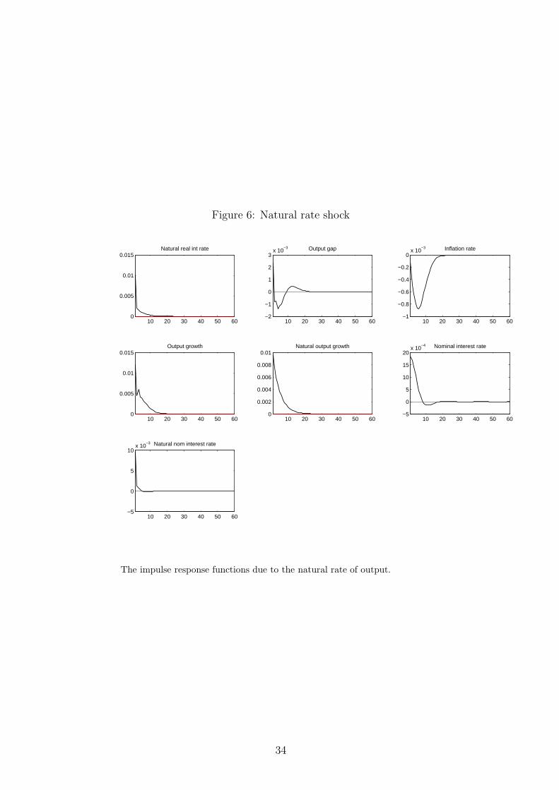
Figure 6: Natural rate shock

10 20 30 40 50 600

0.005

0.01

0.015Natural real int rate

10 20 30 40 50 60−2

−1

0

1

2

3x 10

−3 Output gap

10 20 30 40 50 60−1

−0.8

−0.6

−0.4

−0.2

0x 10

−3 Inflation rate

10 20 30 40 50 600

0.005

0.01

0.015Output growth

10 20 30 40 50 600

0.002

0.004

0.006

0.008

0.01Natural output growth

10 20 30 40 50 60−5

0

5

10

15

20x 10

−4 Nominal interest rate

10 20 30 40 50 60−5

0

5

10x 10

−3 Natural nom interest rate

The impulse response functions due to the natural rate of output.

34