Keynesian Dynamics and the Wage-Price Spiral. Estimating ...

Keynesian Dynamics and the Wage-Price Spiral.Estimating and Analyzing

a Baseline Disequilibrium Approach

Pu ChenFaculty of Economics

Bielefeld University, BielefeldGermany

Carl ChiarellaSchool of Finance and EconomicsUniversity of Technology, Sydney

Australia

Peter FlaschelFaculty of EconomicsBielefeld University

Germany

Willi SemmlerFaculty of Economics

Bielefeld University, BielefeldGermany

November 10, 2004

Abstract:

In this paper, we reformulate the theoretical baseline DAS-AD model of Asada, Chen, Chiarella andFlaschel (2004) to allow for its somewhat simplified empirical estimation. The model now exhibits aTaylor interest rate rule in the place of an LM curve and a dynamic IS curve and dynamic employ-ment adjustment. It is based on sticky wages and prices, perfect foresight of current inflation ratesand adaptive expectations concerning the inflation climate in which the economy is operating. The im-plied nonlinear 6D model of real markets disequilibrium dynamics avoids striking anomalies of the oldNeoclassical synthesis and can be usefully compared with the model of the new Neoclassical Synthesiswhen the latter is based on both staggered prices and wages. It exhibits typical Keynesian feedbackstructures with asymptotic stability of its steady state for low adjustment speeds and with cyclical lossof stability – by way of Hopf bifurcations – when certain adjustment speeds are made sufficiently large.

In the second part we provide system estimates of the equations of the model in order to study itsstability features based on empirical parameter estimates with respect to its various feedback channels.Based on these estimates we find that the dynamics is strongly convergent around the steady state,but will loose this feature if the inflationary climate variable adjusts sufficiently fast. We also studyto which extent more active interest rate feedback rules or downward wage rigidity can stabilize thedynamics in the large when the steady state is made locally repelling by a faster adjustment of infla-tionary expectations. We find support for the orthodox view that (somewhat restricted) money wageflexibility is the most important stabilizer in this framework, while monetary policy should allow forsufficient steady state inflation in order to avoid stability problems in areas of the phase space wherewages are still not very flexible in a downward direction.

———————Keywords: DAS-DAD growth, wage and price Phillips curves, nonlinear estimation, stability, economicbreakdown, persistent cycles, monetary policy.

JEL CLASSIFICATION SYSTEM: E24, E31, E32.

1

1 Introduction

In this paper, we reformulate, simplify and also extend from the empirical perspective amature, but traditionally oriented theoretical model of disequilibrium AS-AD dynamicswith both traditional, but also quite recent microfoundations, as for example providedin Blanchard and Katz’ (1999) analysis of the dynamics of money wages. Our model ofnow in fact D(isequilibrium)AS-D(isequilibrium)AD growth is in its qualitative featuresbased on our earlier theoretical presentation and analysis of a model of DAS-AD growthdynamics, and represents a significant reformulation of the conventional neoclassical AS-AD framework, see Asada, Chen, Chiarella, Flaschel (2004) for details. It replaces theLM curve of the earlier paper by a Taylor interest rate policy rule, as in the New Key-nesian approaches. The model, as well as its theoretical analog, exhibits sticky wages aswell as sticky prices, underutilized labor as well as capital stock, myopic perfect foresightof current wage and price inflation rates and adaptively formed medium-run calculationsconcerning the inflation climate in which the economy is operating. Moreover we nowemploy a dynamic IS-equation in the place of the originally static one of the Asada,Chen, Chiarella, Flaschel (2004) paper and will also make use of a dynamic form ofOkun’s law in addition.

The resulting nonlinear 5D model of labor and goods market disequilibrium dynamics(with a Taylor rule based treatment of the financial part of the economy) avoids thestriking anomalies of the conventional AS-AD model of the old Neoclassical synthesiswhen analyzed under the assumption of myopic perfect foresight.1 Instead it exhibitsKeynesian feedback dynamics proper with in particular asymptotic stability of its uniqueinterior steady state solution for low adjustment speeds of wages, prices, and expectationsamong others. The loss of stability occurs cyclically, by way of Hopf bifurcations, whensome of these adjustment speeds are made sufficiently large, even leading eventually topurely explosive dynamics sooner or later. This latter fact – if it occurs – implies theneed to look for appropriate extrinsic (behavioral) nonlinearities that can bound thedynamics in an economically meaningful domain, such as (some) downward rigidity ofwages and prices and the like, if the economy departs too much from its steady stateposition. This procedure of making an explosive dynamics bounded and thus viablestands in stark contrast to the New Keynesian approach to macrodynamics where on asimilar level of formalization total instability is desirable and achieved by the choice ofan appropriate Taylor policy rule and where the economy is then made a bounded onesimply by assumption (and thus always sitting in the steady state if exogenously givenstochastic processes are removed from the dynamics).

Our approach is indeed – formally seen – closely related to the New Keynesian one. Weuse the same formal structure for the variables that drive wage and price inflation rates(utilizations rates and real wages), but with a microfoundations that are for examplebased on Blanchard and Katz’s (1999) reconciliation of Wage Phillips Curves and currentlabor market theories. The basic difference in the wage-price module is on this basis thatwe augment this structure by hybrid expectations formation where the forward-lookingpart is based on a neoclassical type of dating and where expectations are of cross-over

1These anomalies include in particular saddle point dynamics that imply instability unless somepoorly motivated – and indeed inconsistent – jumps are imposed on certain variables, here in fact onboth the price and the wage level, despite the existence of a money wage Phillips Curve (WPC), seeAsada, Chen, Chiarella and Flaschel (2004) for details.

2

type, i.e., we have price inflation expectations in the Wage Phillips Curve (WPC) andwage inflation expectations in the Price Phillips Curve (PPC). Our formulation of thewage-price module allows therefore an interesting comparison to situations where NewKeynesian authors allow for both staggered prices and wages. Concerning the IS-curvewe make use of a law of motion for the rate of capacity utilization of firms that dependson the level of capacity utilization (the dynamic multiplier), the real rate of interestand finally on the real wage and thus on income distribution. New Keynesian authorsgenerally use a purely forward-looking IS-curve (with only the real rate of interest effect),a procedure that – like the purely forward-looking New Keynesian Phillips curve – hasbeen criticized from the empirical point of view, see in particular the recent paper byFuhrer and Rudebusch (2004) with regard to the relevance of forward-looking behaviorin the IS-representation of goods-market dynamics. Since we distinguish between therate of employment of the labor force and that of the capital stock, the rate of capacityutilization, we finally employ some form of Okun’s law to relate these to variables witheach other.

The model of this paper can therefore, on the one hand, usefully compared to theNew Keynesian one with staggered wage and price dynamics, but is on the other handradically different from this approach with respect to implications, since we are notforced into a framework with four forward-looking variables where we have to look forfour unstable roots in order to get the conclusion that the model is always sitting inits steady state (assuming boundedness as solution procedure) as long as only isolatedshocks occur and is thus driven as far as business cycle implications are concerned solelyby the stochastic processes that are added to its deterministic core. We have forward-looking behavior (with neoclassical dating) and will find asymptotic stability in thetraditional sense of the word over certain ranges in the parameter space, while – in thecase of local instability – we look for behavioral nonlinearities that allow the dynamicsto remain bounded in an economically meaningful range in the place of an impositionof such boundedness on admissible solution curves and looking for determinacy.

We, by contrast, therefore obtain and can prove – still from the purely theoretical per-spective – based on empirically still unrestricted sizes of the considered adjustmentspeeds of wages, prices, and quantities, the existence of damped, persistent or explosivefluctuations in the real and the nominal part of the dynamics, in the rates of capacityutilization of both labor and capital, and of wage and price inflation rates which hereinduce interest rate adjustments by the monetary authority through the attempt to sta-bilize the observed output and price level fluctuations, providing us with a Keynesiantheory of an income distribution driven cycle, including a modern approach to monetarypolicy in such a context. This even holds in the case of myopic perfect foresight, wherethe structure of the od Neoclassical synthesis radically dichotomizes into independentclassical supply-side and real dynamics – that cannot be influenced by monetary policy –and a subsequently determined inflation dynamics, that are purely explosive if the pricelevel is taken as a predetermined variable, a situation that forces conventional approachesto these dichotomizing dynamics to assume convergence by an inconsistent applicationof the jump-variable technique,2 see again Asada, Chen, Chiarella and Flaschel (2004)for details. In our new matured type of Keynesian labor and goods market dynamicswe however can treat myopic perfect foresight of both firms and wage earners without

2since the nominal wage is transformed into a non-predetermined variable there, despite the initialassumption of only gradually adjusting money wages.

3

the need for the methodology of this ‘rational expectations’ solution in the context ofan unstable saddlepoint dynamics, be it of old or new Keynesian type.

From the global perspective, if our theoretical model loses asymptotic stability for higheradjustment speeds, in the present framework specifically of prices and our inflationaryclimate expression, purely explosive behavior is the generally observed outcome, as itcan be demonstrated by means of numerical simulations. The considered, so far onlyintrinsically nonlinear, model type therefore cannot be considered as being completelyspecified under such circumstances, since some mechanism is then required to boundthe fluctuations to economically viable regions. Downward money wage rigidity was themechanism we have often used for this purpose and which we will try here again (withlimited success however as we shall see), in contrast to its successful application in thenumerical investigations in Asada, Chen, Chiarella and Flaschel (2004).

The here estimated somewhat simplified feedback structure of their theoretical model,now indeed no longer (in general) supports the view (of Keynes and others) that down-ward money wage rigidity will stabilize the economy (as was shown in the structurallymore elaborated earlier paper). Instead, this downward rigidity may now even causeeconomic breakdown when applied to situations that were strongly stable (convergentto the steady state) without it. This is due to our estimation of the dynamics of capacityutilization rates where we find, on the one hand, besides the usual negative dependenceon the real rate of interest, a strong negative dependence on the real wage. On the otherhand, we find in the wage-price block of the model the sign restrictions of New Keynesianwage and price inflation equations (but do not have their sign reversals in their reduced-form expressions later on, due to our different handling of forward-looking expectationsand the inclusion of backward-looking ones). As far as the money wage Phillips curveis concerned we also confirm the form specified in Blanchard and Katz (1999) and finda similar general form to hold for the price inflation Phillips curve. These estimatedcurves then by and large suggest that real wage changes depend positively on economicactivity, and this the more the stronger nominal wages react to the employment gap onthe market for labor. In sum we therefore get that growth rate of real wages dependsnegatively on its level, and this stabilizing feedback chain to being the stronger the moreflexible nominal wages react to labor market imbalances in the upward as well as in thedownward direction. Complete downward wage flexibility may therefore become a prob-lem, and this already in situations where the economy is producing fairly damped cycles(if the monetary authority is using too low an inflation target).

In the numerical simulations of the estimated model we will indeed then find that thereestablishment of money wage flexibility in severely depressed regions of the phase space(however coupled with some midrange downward wage rigidity) will avoid this break-down, however at the costs of persistent economic fluctuations to some extent belowthe normal operating level of the economy. In the present framework (of a profit-ledgoods demand regime, where real wage increases decrease economic activity) finally es-tablished downward money wage flexibility is therefore good for economic stability andthis the more the closer this stability feature is established to the steady state from be-low. The opposite conclusion however holds with respect to price flexibility. Excludingby our parameter estimates significant price level deflation – but not wage level defla-tion – from occurring, we thereby obtain and study a baseline model of the DAS-DADvariety with a rich set of stability implications and with various types of business cy-cle fluctuations that it can generate endogenously as well as exogenously (by adding

4

stochastic processes to the considered deterministic dynamics). The dynamic outcomesof this baseline disequilibrium AS-AD or DAS-DAD model can be usefully contrastedwith those of the currently fashionable New Keynesian alternative (the new NeoclassicalSynthesis) that in our view is more limited in scope, at least as far as the treatment of in-teracting Keynesian feedback mechanisms and the thereby implied dynamic possibilitiesare concerned. A detailed comparison with this New Keynesian approach is providedin Chiarella, Flaschel and Franke (2004, Ch.1). This comparison reveals in particularthat one does not really need the typical (in our view strange) dynamics of rational ex-pectation models, based on the specification of certain forward looking variables, if suchforward-looking behavior is coupled with backward-looking behavior for the medium-run evolution of the economy (and neoclassical dating in the forward-looking part) andif certain non-linearities in economic behavioral make the obtained dynamics boundedfar off the steady state. In our approach standard Keynesian feedback mechanisms arecoupled with a wage-price spiral having – besides partial forward-looking behavior – aconsiderable degree of inertia, with the result that these feedback mechanisms by andlarge work as expected (as known from partial analysis), in their interaction with theadded wage and price level dynamics.

The present paper therefore intends to provide a empirically supported baseline modelof the Keynesian DAS-DAD variety, not plagued by the theoretical anomalies of the oldNeoclassical Synthesis and the empirical anomalies of the new Neoclassical Synthesisof the New Keynesian approach. It does so on the basis of the fully specified DAS-AD growth dynamics of Asada, Chen, Chiarella and Flaschel (2004), by transformingthese dynamics into a reduced DAS-DAD format that can be estimated empirically.It discusses the feedback structure of this reduced form and its stability implications,first on a general level and then on the level of the sign and size restrictions obtainedfrom empirical estimates of the six laws of motion of the dynamics. These estimates alsoallow us to show asymptotic stability for the estimated parameter sizes and to determinestability boundaries (with respect to the speed of adjustment of the inflationary climate)where the need for further (behavioral) nonlinearities therefore becomes a matter offact, here only studied to a certain degree, but further investigated and discussed in acompanion paper to the present one (see Asada, Chiarella, Flaschel and Hung, 2004).

Section 2 considers for later comparison the New Keynesian macrodynamic model withstaggered wage and price setting in a deterministic and continuous time framework.Section 3 then presents our reformulation of the baseline Keynesian DAS-AD growthdynamics of Asada, Chen, Chiarella and Flaschel (2004) as a DAS-DAD growth dynamicsin order to make this model applicable to empirical estimation. Section 4 considersthe feedback chains of the reformulated model and derives cases of local asymptoticstability and of loss of stability by way of Hopf-bifurcations. In section 5 we thenestimate the model to find out sign and size restrictions for its behavioral equationsand which type of feedback mechanisms may apply to the US-economy after World WarII. Section 6 investigates in detail the stability properties of the estimated dynamics.Section 7 analyzes on the one hand the stability problems that occur when there is afloor to money wage deflation and the role of monetary policy in such a context. Onthe other hand, it studies the role of such a floor and its removal in more or less severedepressions from the global point of view, when the steady state becomes a local repellerdue to a faster , adjustment of the inflationary climate expression considered to surroundcurrent perfectly foreseen inflation. We here find that the combination of some downward

5

rigidity in wage deflation coupled with its returning flexibility when depressions becomesufficiently severe will on the one hand avoid the explosive fluctuations of the completelyunrestricted case, while also avoiding complete the economic collapse that would comeabout when the floor to wage deflation would be a global one. Section 8 concludes.Details of the estimation results are presented in an appendix to the paper.

2 New Keynesian macrodynamics

In this section we consider briefly the modern analog to the old neoclassical synthesis(in its Keynesian format), the New Keynesian approach to macrodynamics, and thisalready in its advanced form, where both staggered price setting and staggered wagesetting are assumed. We here follow Woodford (2003, p.225) and Ereg et al. (2000) intheir formulation of staggered wages and prices, where their joint evolution is coupledwith the usual forward-looking output dynamics, coupled with a derived law of motionfor real wages now in addition.3 We shall only briefly look at this extended approachhere in order to allow us to consider the similarities and differences between our laterand these New Keynesian dynamics later on.

Woodford (2003, p.225) makes basically use of the following two loglinear equations fordescribing the joint evolution of wages and prices:4

∆ ln wtWPC= βEt(∆ ln wt+1) + βwy ln Yt − βwω ln ωt

∆ ln ptPPC= βEt(∆ ln pt+1) + βpy ln Yt + βpω ln ωt

where all parameters are assumed as positive. Our first aim here is to derive the con-tinuous time analog to these two equations (and the other equations of the full model)and to show on this basis how this extended model is solved in the spirit of the rationalexpectations school.

In a deterministic setting we obtain from the above

∆ ln wt+1WPC=

1

β[∆ ln wt − βwy ln Yt + βwω ln ωt]

∆ ln pt+1PPC=

1

β[∆ ln pt − βpy ln Yt − βpω ln ωt]

and thus get, if we assume (in all of the following and without much loss in generality)that the parameter β is not only close to one, but in fact set equal to one:

∆ ln wt+1 −∆ ln wtWPC= −βwy ln Yt + βwω ln ωt

∆ ln pt+1 −∆ ln ptPPC= −βpy ln Yt − βpω ln ωt

Denoting by πw the rate of wage inflation and by πp the rate of price inflation (bothindexed by the end of the corresponding period) then gives rise to (when transferred tocontinuous time, with ln Y = y and θ = ln ω):

3Further approaches that incorporate both wage and price staggering are provided in Christiano,Eichenbaum and Evans (2001) and Sbordone (2001, 2002).

4∆ the backward oriented difference operator.

6

πw WPC= −βwyy + βwωθ

πp PPC= −βpyy − βpωθ

With respect to the output dynamics of the New Keynesian approach:

yt = yt+1 − αyi(it − πpt+1 − i0), i.e., yt+1 − yt = αyi(it − πp

t+1 − i0)

we get on this basis the reduced form law of motion

yIS= αyi[(βiπ − 1)πp + (βiy + βpy)y + βpωθ)]

where we have already inserted an interest rate policy rule in order to (hopefully) getdeterminacy as in the New Keynesian baseline model, which is known to be indeterminedfor the case of an interest rate peg. As Taylor interest rate policy rule we here have chosenthe simple rule:

i = it = io + βiππ + βiyy

see Walsh (2003, p.247), which is of a classical Taylor rule type.

There remains finally the law of motion for real wages to be determined, which due toθ = ln ω simply reads

θ = πw − πp

We thus get from this extended New Keynesian model an autonomous linear dynam-ics, in the variables πw, πp, y and θ. The in general uniquely determined steady stateof the dynamics is given by (0.0, 0, io). From the definition of θ we obtain, in directgeneralization of the baseline New Keynesian model with only staggered price setting,that the model exhibits four forward-looking variables. Searching for a zone of determi-nacy of the dynamics (appropriate parameter values that make the steady state the onlybounded solution of the dynamics to which the economy then immediately returns afterisolated shocks of any type) thus demands to establish conditions such that all roots ofthe Jacobian have positive real parts.

The Jacobian of the 4D dynamical system under consideration reads:

J =

0 0 −βwy βwω

0 0 −βpy −βpω

0 αyi(βiπ − 1) αyi(βiy + βpy) αyiβpω

1 −1 0 0

.

7

For the determinant of this Jacobian we therefrom get

−|J | = (βwyβpω + βpyβwω)αyi(βiπ − 1)>=<

0 iff βiπ>=<

1

We thus get that an active monetary policy (βiπ > 1) is no longer appropriate to ensuredeterminacy (for which a positive determinant of J is a necessary condition). Therearises the necessity to specify an extended interest rate policy rule from which one canobtain determinacy (the steady state as the only stable solution and the only realizedsituation in this deterministic setup) as in the New Keynesian baseline model, whichis known to be indetermined in the case of an interest rate peg, but which is alwaysdetermined for βiπ > 1.

There are a variety of critical arguments raised in the literature against the New PhillipsCurve (NPC) of the baseline model of Keynesian macrodynamics, see in particularMankiw (2001) and recently Eller and Gordon (2003) for particular strong statements.5

These and other criticisms in our view will also apply to the above extended wage andprice dynamics. In view of these and other critiques we here propose the following mod-ifications to the above presentation of the wage-price dynamics which will remove fromit completely the questionable feature of a sign reversal for the role of output and wagegaps, caused by the fact that future values of the considered state values are used onthe right hand side of their determining equations, which implies that the time ratesof change of these variables depend on output and wage gaps with a reversed sign infront on them. These sign reversals are at the root of the problem when the empiri-cal relevance of such NPC’s is investigated. We instead will make use of the followingexpectations augmented wage and price Phillips curves:

∆ ln wt+1WPC= κw∆ ln pt+1 + (1− κw)πm

t + βwy ln Yt − βwω ln ωt]

∆ ln pt+1PPC= κp∆ ln wt+1 + (1− κp)π

mt + βpy ln Yt + βpω ln ωt]

We have modified the New Keynesian approach to wage and price dynamics here onlywith respect to the terms that concern expectations, in order to obtain the situationof in fact a wage-price spiral from it. We first assume that expectation formation isof a crossover type, with perfectly foreseen price inflation in the WPC of workers andperfectly foreseen wage inflation in the PPC of firms. Furthermore, we make use inthis regard of a neoclassical dating in the considered PC’s, which means that – as inthe reduced form PC then often considered – we have the same dating for expectationsand actual wage and price formation on both sides of the PC’s. Finally, followingChiarella and Flaschel (1996), we assume expectations formation to be of a hybrid type,where a certain weight is given to current (perfectly foreseen) inflation rates and thecounterweight attached to a concept which we have dubbed the inflationary climateπm that is surrounding the currently evolving wage-price spiral. We thus assume thatworkers as well as firms to a certain degree pay attention of whether the current situationis embedded in a high inflation regime or in a low inflation one.

5With respect to the New Phillips curve it is stated in Mankiw (2001): ”Although the new KeynesianPhillips curves has many virtues, it also has one striking vice: It is completely at odd with the facts.”

8

These relatively straightforward modifications of the New Keynesian approach to ex-pectations formation will imply for the dynamics of what we call a matured traditionalKeynesian approach – completed in the next section – radically different solutions andstability features, with in particular no need to single out the steady state as the onlyrelevant situation for economic analysis in the deterministic setup here considered. Con-cerning microfoundations for the assumed wage-price spiral we here only note that theWPC can be microfounded as in Blanchard and Katz (2000), using standard labor mar-ket theories, giving rise to nearly exactly the form shown above (with the unemploymentgap in the place of the logarithm of the output gap) if hybrid expectations formation isembedded into their approach in addition. Concerning the PPC a similar procedure maybe applied based on desired markups of firms. Along these lines one in particular getsan economic motivation for the inclusion of – indeed the logarithm – of the real wage (orwage share) with negative sign into the WPC and with positive sign into the PPC, with-out any need for loglinear approximations. We furthermore use the (un-)employmentgap and the capacity utilization gap in these two PC’s, respectively, in the place of asingle measure (the log of the output gap). We conclude that the above wage-pricespiral is an interesting alternative to the – theoretically rarely discussed and empiricallyquestionable – New Keynesian form of wage-price dynamics. This wage-price spiral willbe embedded into a complete Keynesian approach in the next section, exhibiting a dy-namic IS-equation as in Rudebusch and Svensson (1999), now also including real wageeffects and thus a role for income distribution, exhibiting furthermore Okun’s law as thelink from goods to labor markets and exhibiting of course the classical type of a Taylorinterest rate policy rule in the place of an LM-curve.

3 Keynesian disequilibrium dynamics: Empirically

oriented reformulation of a baseline model

In this section we reformulate the theoretical disequilibrium model of AS-AD growth ofAsada, Chen, Chiarella and Flaschel (2004) in order to make it applicable for empiricalestimation in a somewhat simplified way and for the study of the role of contemporaryinterest rate policy rules in such a framework. We dismiss now the LM curve of theoriginal approach and replace it here by a Taylor type policy rule and use in additiondynamic IS as well as employment equations in the place of the originally static ones,where with respect to the former the dependence of consumption and investment onincome distribution now only appears in an aggregated format. We use Blanchard andKatz (2000) error correction terms both in the wage and the price Phillips curve andthus give income distribution a role to play in wage as well as in price dynamics. Finally,we will have again inflationary inertia in a world of myopic perfect foresight through theinclusion of a medium-run variable, the inflationary climate in which the economy isoperating, and its role for the wage - price dynamics of the considered economy.

We start from the observation that a Keynesian model of aggregate demand fluctuationsshould (independently of whether justification can be found for this in Keynes’ GeneralTheory) allow for under- (or over-)utilized labor as well as capital in order to be generalenough from the descriptive point of view. As Barro (1994) for example observes, IS-LM is (or should be) based on imperfectly flexible wages and prices and thus on theconsideration of wage as well as price Phillips Curves. This is precisely what we will

9

do in the following, augmented by the observation that also medium-run aspects countboth in wage and price adjustments, here formulated in simple terms by the introductionof the concept of an inflation climate. We have moreover model-consistent expectationswith respect to short-run wage and price inflation. The modification of the traditionalAS-AD model that we shall consider thus treats – as already described in the precedingsection – expectations in a hybrid way, with crossover myopic perfect foresight of thecurrently evolving rates of wage and price inflation on the one hand and an adaptiveupdating of an inflation climate expression with exponential or any other weightingschemes on the other hand.

We consequently assume two Phillips Curves in the place of only one. In this way, wecan discuss wage and price dynamics separately from each other, in their structuralforms, now indeed both based on their own measure of demand pressure, namely V l −V l, V c − V c, in the market for labor and for goods, respectively. We here denote byV l the rate of employment on the labor market and by V l the NAIRU-level of thisrate, and similarly by V c the rate of capacity utilization of the capital stock and V c

the normal rate of capacity utilization of firms. These demand pressure influences onwage and price dynamics, or on the formation of wage and price inflation rates, w, p,are both augmented by a weighted average of corresponding cost-pressure terms, basedon forward looking myopic perfect foresight p, w, respectively, and a backward lookingmeasure of the prevailing inflationary climate, symbolized by πm.

We thereby arrive at the following two Phillips Curves for wage and price inflation,which in this core version of Keynesian AS-AD dynamics are – qualitatively seen – for-mulated in a fairly symmetric way.6 We stress that we include forward-looking behaviorhere, without the need for an application of the jump variable technique of the rationalexpectations school in general and the New Keynesian approach in particular as will beshown in the next section.7

The structural form of the wage-price dynamics:

w = βw1(Vl − V l)− βw2(ln ω − ln ωo) + κwp + (1− κw)πm, (1)

p = βp1(Vc − V c) + βp2(ln ω − ln ωo) + κpw + (1− κp)π

m. (2)

Somewhat simplified versions of these two Phillips curves have been estimated for theUS-economy in various ways in Flaschel and Krolzig (2004), Flaschel, Kauermann andSemmler (2004) and Chen and Flaschel (2004) and were found there to represent a signif-icant improvement over the conventional single reduced-form Phillips curve, there withwage flexibility being greater than price flexibility with respect to their demand pressuremeasure in the market for goods and for labor,8 respectively, and with workers being

6With respect to empirical estimation one could also add the role of labor productivity growth,yet will here not do so, but concentrate on the cycle component of the model, caused by changingincome distribution in a world of stable goods market and interest rate dynamics. With respect to thedistinction between real wages, unit wage costs we shall therefore detrend the corresponding time seriessuch that the following types of PC’s can still be applied.

7For a detailed comparison with the New Keynesian alternative to our model type see Chiarella,Flaschel and Franke (2004).

8for lack of better phrases we associate the degree of wage and price flexibility with the size of theparameters βw1 , βp1 , though of course the extent of these flexibilities will also depend on the size of thefluctuations of the excess demands in the market for labor and for goods, respectively.

10

more short-sighted than firms with respect to their cost pressure terms. Note that sucha finding is not possible in the conventional framework of a single reduced-form Phillipscurve. Inflationary expectations over the medium run, πm, i.e., the inflationary climatein which current inflation is operating, may be adaptively following the actual rate ofinflation (by use of some linear or exponential weighting scheme), may be based ona rolling sample (with hump-shaped weighting schemes), or on other possibilities forupdating expectations. For simplicity of the exposition we shall make use of the con-ventional adaptive expectations mechanism in the theoretical part of this paper:

πm = βπm(p− πm) (3)

Note that for our current version of the wage-price spiral, the inflationary climate variabledoes not matter for the evolution of the real wage ω = w/p , the law of motion of whichis given by (with κ = 1/(1− κwκp)):

ω = κ[(1− κp)(βw1(Vl − V l)− βw2(ln ω − ln ωo))− (1− κw)(βp1(V

c − V c) + βp2(ln ω − ln ωo))]

This follows easily from the following obviously equivalent representation of the abovetwo PC’s:

w − πm = βw1(Vl − V l)− βw2(ln ω − ln ωo) + κw(p− πm),

p− πm = βp1(Vc − V c) + βp2(ln ω − ln ωo)) + κp(w − πm),

by solving for the variables w− πm and p− πm. It also implies the following two across-markets or reduced form PC’s:

p = κ[βp1(Vc − V c) + βp2(ln ω − ln ωo) + κp(βw1(V

l − V l)− βw2(ln ω − ln ωo))] + πm,

w = κ[βw1(Vl − V l)− βw2(ln ω − ln ωo)) + κw(βp1(V

c − V c) + βp2(ln ω − ln ωo))] + πm,

which represent a considerable generalization of the conventional view of a single-marketprice PC with only one measure of demand pressure, the one in the labor market.

The remaining laws of motion of the private sector of the model are as follows:

V c = −αV c(V c − V c)± αω(ln ω − ln ωo)− αr((r − p)− (ro − π)) (4)

V l = αV l1(V c − V c) + αV l

2V c (5)

The first law of motion is of the type of a dynamic IS-equation, see also Rudebuschand Svensson (1999) in this regard, here represented by the growth rate of the capacityutilization rate of firms. It reflects the dependence of output changes on aggregate incomeand thus on the rate of capacity utilization by assuming a negative, i.e., stable dynamicmultiplier relationship in this respect, it shows the joint dependence of consumptionand investment on the real wage (which in the aggregate may in principle allows for

11

positive or negative signs before the parameter αω, depending on whether consumptionor investment is more responsive to real wage changes), and shows finally the negativeinfluence of the real rate of interest on the evolution of economic activity. Note herethat we have generalized this law of motion in comparison to the one in the originalbaseline model of Asada, Chen, Chiarella and Flaschel (2004), since we now allow for thepossibility that also consumption, not only investment, depends on income distributionas measured by the real wage. We note that we also use ln ω in the dynamic multiplierequation, since this variable will be used later on to estimate this equation.

In the second law of motion, for the rate of employment, we assume that the employmentpolicy of firms follows – in the form of a generalized Okun Law – the rate of capacityutilization (and the thereby implied rate of over- or underemployment of the employedworkforce) partly with a lag (measured by 1/βV l

1), and partly without a lag (through a

positive parameter αV l2). Employment is thus assumed to adjust to the level of current

activity in somewhat delayed form which is a reasonable assumption from the empiricalpoint of view. The second term, αV l

2V c, is added to take account of the possibility that

Okun’s Law may hold in level form rather than in the form of a law of motion, sincethis latter dependence can be shown to be equivalent to the use of a term (V c/V c)

αV l2

when integrated, i.e., the form of Okun’s law in which this law was originally specifiedby Okun (1967) himself.

The above two laws of motion therefore reformulate the static IS-curve and the employ-ment this curve implies, as employed in Asada, Chen, Chiarella and Flaschel (2004),in a dynamic form. They only reflect implicitly the there assumed dependence of therate of capacity utilization on the real wage, due to on smooth factor substitution inproduction (and the measurement of the potential output this implies in Asada, Chen,Chiarella and Flaschel (2004))), which constitutes another positive influence of the realwage on the rate of capacity utilization and its rate of change. This simplification helpsto avoid the estimation of separate equations for consumption and investment C, I andfor potential output Y p as they were discussed and used in detail in this earlier paper.

Finally, we no longer to employ here a law of motion for real balances as was still the casein Asada, Chen, Chiarella and Flaschel (2004). Money supply is now accommodatingto the interest rate policy pursued by the central bank and thus does not feedback intothe core laws of motion of the model. As interest rate policy we assume the followingclassical type of Taylor rule:

r = −γr(r − ro) + γp(p− π) + γV c(V c − V c) (6)

Note that we allow for interest rate smoothing in this rule. Furthermore, the actual(perfectly foreseen) rate of inflation p is used to measure the inflation gap with respectto the inflation target π of the central bank. There is in addition the assumption of apositive influence of an output gap in the law of motion for the nominal rate of interest,here measured by the rate of excess capacity of firms. Note finally that we could haveincluded (but have not done this here yet) a new kind of gap into the above Taylor rule,the real wage gap, since we have in our model a dependence of aggregate demand onincome distribution and the real wage. The state of income distribution matters for the

12

dynamics of our model and thus should also play a role in the decisions of the centralbank. All of the employed gaps are measured relative to the steady state of the model,in order to allow for an interest rate policy that is consistent with it.

We note that the steady state of the considered dynamics is basically the same asthe one considered in Asada, Chen, Chiarella and Flaschel (2004), with εo = 0, V c

o =V c, V l

o = V l, πmo = π. The values of ωo, ro are in principle determined as in Asada,

Chen, Chiarella and Flaschel (2004), but are here just assumed as given, underlying thelinear approximation of the IS curve of the present model around the steady state ofthe original framework (when adjusted to the considered modifications of the baselinemodel). As the model is formulated now it exhibits five gaps, to be closed in the steadystate and has five laws of motion, which when set equal to zero, exactly imply this result,since the determinant of the Jacobian of the dynamics is shown to be always non-zeroin the next section of the paper.

The steady state of the dynamics is locally asymptotically stable under certain sluggish-ness conditions that are reasonable from a Keynesian perspective, loses its asymptoticstability by way of cycles (by way of so-called Hopf-bifurcations) if the system becomestoo flexible, and becomes sooner or later globally unstable if (generally speaking) ad-justment speeds become too high, as we shall show below. If the model is subject toexplosive forces, it requires extrinsic nonlinearities in economic behavior – like down-ward money wage rigidity – to come into being at least far off the steady state in orderto bound the dynamics to an economically meaningful domain in the considered 5Dstate space. Asada, Chiarella, Flaschel and Hung (2004) provide a variety of numericalstudies for such an approach with extrinsically motivated nonlinearities and thus under-take its detailed numerical investigation. In sum, therefore, our dynamic AS-AD growthmodel here and there will exhibit a variety of features that are much more in line witha Keynesian understanding of the characteristics of the trade cycle than is the case forthe conventional modelling of AS-AD growth dynamics or its radical reformulation bythe New Keynesians (where – if non-determinacy can be avoided by the choice of anappropriate Taylor rule – only the steady state position is a meaningful solution in therelated setup we considered in the preceding section).

Taken together the model of this section consists of the following five laws of motion(with the derived reduced form expressions as far as the wage-price spiral is concernedand with reduced form expressions by assumption concerning the goods and the labormarket dynamics):9

9As the model is formulated we have no real anchor for the steady state rate of interest (via investmentbehavior and the rate of profit it implies in the steady state) and thus have to assume here that it isthe monetary authority that enforces a certain steady state values for the nominal rate of interest.

13

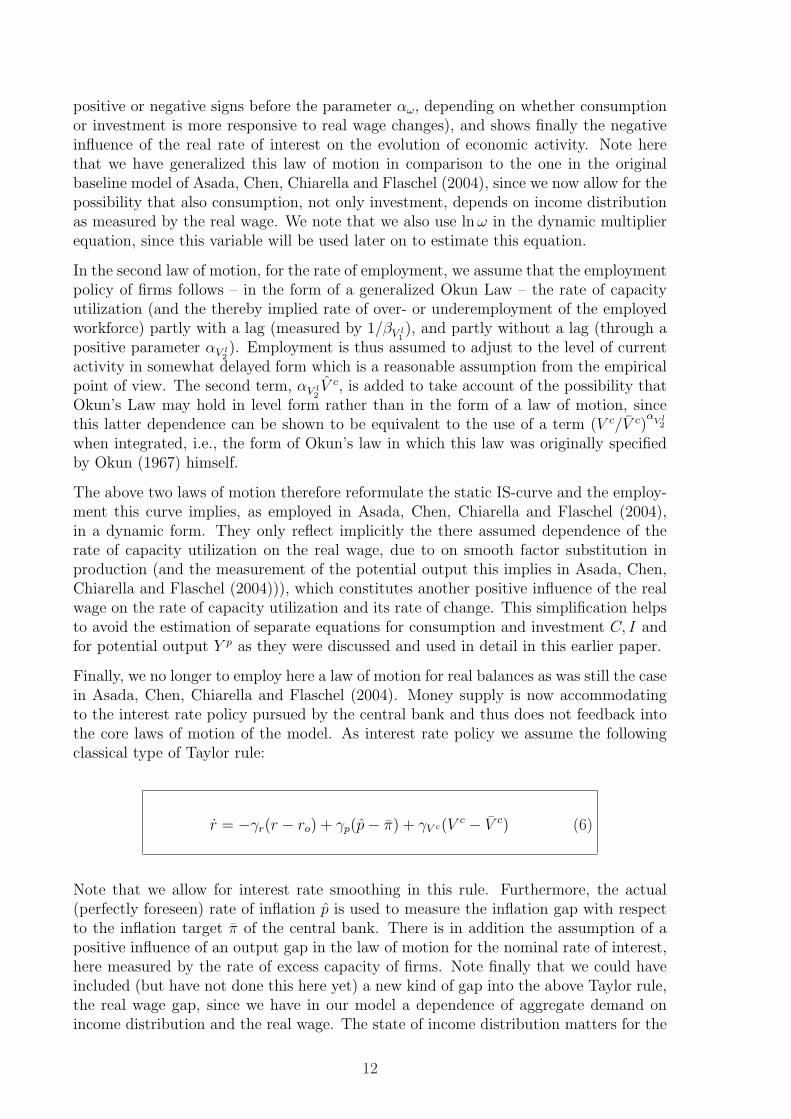
V c Dyn.IS= −αV c(V c − V c)± αω(ln ω − ln ωo)− αr((r − p)− (ro − π)) (7)

V l O.Law= βV l

1(V c − V c) + βV l

2V c (8)

rT.Rule

= −γr(r − ro) + γp(p− π) + γV c(V c − V c) (9)

ωRWPC

= κ[(1− κp)(e¯taw1(V

l − V l)− βw2(ln ω − ln ωo))

− (1− κw)(βp1(Vc − V c) + βp2(ln ω − ln ωo))] (10)

πm I.Climate= βπm(p− πm) or (11)

πm(t) = πm(to)e−βπm (t−to) + βπm

∫ t

to

eβπm (t−s)p(s)ds

representing in correspondence to the baseline model of New Keynesian macroeconomicsthe IS-dynamics, Okun’s Law and the Taylor Rule, but including now also the dynamicsof the real wage, and the updating of the inflationary climate expression. We have tomake use in addition of the following reduced form expression for the price inflation rateor the PPC:

p = κ[βp1(Vc − V c) + βp2(ln ω − ln ωo)

+ κp(βw1(Vl − V l)− βw2(ln ω − ln ωo))] + πm (12)

which has to be inserted into the above laws of motion in various places in order to getan autonomous nonlinear system of differential equations in the state variables: capacityutilization V c, the rate of employment V l, the nominal rate of interest r, the real wagerate ω, and the inflationary climate expression πm. We stress that one can consider theeq. (12) as a sixth law of motion of the considered dynamics which however – whenadded — leads a system determinant which is zero and which therefore allows for zero-root hysteresis for certain variables of the model (in fact in the price level if the targetrate of inflation of the CB is zero and if interest rate smoothing is present in the TR).We have written the laws of motion in an order that first presents the dynamic equationsalso present in the baseline New Keynesian model of inflation dynamics, and then ourformulation of the dynamics of income distribution and of the inflationary climate inwhich the economy is operating.

With respect to the empirically motivated restructuring of the original theoretical frame-work, the model is as pragmatic as the approach employed by Rudebusch and Svensson(1999). By and large we believe that it represents a working alternative to the NewKeynesian approach, in particular when the current critique of the latter approach istaken into account. It overcomes the weaknesses and the logical inconsistencies of theold Neoclassical synthesis, see Asada, Chen, Chiarella and Flaschel (2004), and it doesso in a minimal way from a mature, but still traditionally oriented Keynesian perspective(and is thus not really ’New’). It preserves the problematic stability features of the realrate of interest channel, where the stabilizing Keynes effect or the interest rate policyof the central bank is interacting with the destabilizing, expectations driven Mundell

14

effect. It preserves the real wage effect of the old Neoclassical synthesis, where – due toan unambiguously negative dependence of aggregate demand on the real wage – we hadthat price flexibility was destabilizing, while wage flexibility was not. This real wagechannel is not really a topic in the New Keynesian approach, due to the specific form ofwage-price dynamics there considered, see the preceding section, and it is summarizedin the figure 1 for the situation where investment dominates consumption with respectto real wage changes. In the opposite case, the situations considered in this figure willbe reversed with respect to their stability implications.

AssetMarkets:

DepressedGoods Markets

DepressedLabor Markets

wages

prices

Normal Rose Effect (example):

interest rates

investment

aggregate demand

Recovery!

Recovery!

real wages

consumption

?

AssetMarkets:

DepressedGoods Markets

DepressedLabor Markets

wages

prices

Adverse Rose Effect (example):

interest rates

investment

aggregate demand

Further

Further

real wages

consumption

?

Figure 1: Rose effects: The real wage channel of Keynesian macrodynamics .

The feedback channels just discussed will be the focus of interest in the now followingstability analysis of our D(isquilibrium)AS-D(isquilibrium)AD dynamics. We have em-ployed reduced-form expressions in the above system of differential equations wheneverpossible. We have thereby obtained a dynamical system in five state variables that is ina natural or intrinsic way nonlinear (to its reliance on growth rate formulations). Wenote that there are many items that reappear in various equations, or are similar to eachother, implying that stability analysis can exploit a variety of linear dependencies in thecalculation of the conditions for local asymptotic stability. This dynamical system willbe investigated in the next section in somewhat informal terms with respect to somestability assertions it gives rise to. A rigorous proof of local asymptotic stability and itsloss by way of Hopf bifurcations can be found in Asada, Chen, Chiarella and Flaschel(2004), there for the original baseline model. For the present model variant we supplya more detailed stability proofs in Asada, Chiarella, Flaschel and Hung (2004), wherealso more detailed numerical simulations of the model will be provided.

4 5D Feedback-guided stability analysis

In this section we illustrate an important method to prove local asymptotic stabilityof the interior steady state of the dynamical system (7) – (11) (with eq. (12) wher-

15

ever needed) through partial motivations from the feedback chains that characterizethis empirically oriented baseline model of Keynesian dynamics. Since the model isan extension of the standard AS-AD growth model, we know from the literature thatthere is a real rate of interest effect typically involved, first analyzed by formal methodsin Tobin (1975), see also Groth (1992). Instead of the stabilizing Keynes-effect, basedon activity-reducing nominal interest rate increases following price level increases, wehave here however a direct steering of economic activity by the interest rate policy ofthe central bank. Secondly, if the correctly anticipated short-run real rate of interest isdriving investment and consumption decisions (increases leading to decreased aggregatedemand), there is the activity stimulating (partial) effect of increases in the rate of infla-tion (as part of the real rate of interest channel) that may lead to accelerating inflationunder appropriate conditions. This is the so-called Mundell-effect that normally worksopposite to the Keynes-effect, but through the same real rate of interest channel as thislatter effect. Due to our use of a Taylor rule in the place of the conventional LM curve,the Keynes-effect is here implemented in a more direct way towards a stabilization ofthe economy (coupling nominal interest rates directly with the rate of price inflation)and it is supposed to work the stronger the larger the parameters γp, γV c are chosen.The Mundell-effect by contrast is the stronger the faster the inflationary climate adjuststo the present level of price inflation, since we have a positive influence of this climatevariable both on price as well as on wage inflation and from there on rates of employmentof both capital and labor.

There is a further important potentially (at least partially) destabilizing feedback mech-anism as the model is formulated. Excess profitability depends positively on the rateof return on capital and thus negatively on the real wage ω. We thus get – since con-sumption may also depend (positively) on the real wage – that real wage increases candepress or stimulate economic activity depending on whether investment or consumptionis dominating the outcome of real wage increases (we here neglect the stabilizing role ofthe additional Blanchard and Katz type error correction mechanisms). In the first case,we get from the reduced-form real wage dynamics:

ω = κ[(1− κp)βw(V l − V l)− (1− κw)βp(Vc − V c)].

that price flexibility should be bad for economic stability, due to the minus sign infront of the parameter βp, while the opposite should hold true for the parameter thatcharacterizes wage flexibility. This is a situation as it was already investigated in Rose(1967). It gives the reason for our statement that wage flexibility gives rise to normaland price flexibility to adverse Rose effects as far as real wage adjustments are con-cerned (if it is assumed – as in our theoretical baseline model – that only investmentdepends on the real wage). Besides real rate of interest effects, establishing opposingKeynes- and Mundell-effects, we thus have also another real adjustment process in theconsidered model where now wage and price flexibility are in opposition to each other,see Chiarella and Flaschel (2000) and Chiarella, Flaschel, Groh and Semmler (2000) forfurther discussion of these as well as of other feedback mechanisms of such Keynesiangrowth dynamics. We observe again that our theoretical DAS-AD growth dynamics inAsada, Chen, Chiarella and Flaschel (2004) – due to their origin in the baseline modelof the Neoclassical Synthesis, stage I – allows for negative influence of real wage changeson aggregate demand solely, and thus only for cases of destabilizing wage level flexibility,but not price level flexibility. In the empirical estimation of the model (7) – (11) we willindeed find that this case seems to be the one that characterizes our empirically and

16

broader oriented dynamics (7) – (11).

This adds to the description of the dynamical system (7) – (11) whose stability prop-erties are now to be investigated by means of varying adjustment speed parametersappropriately. With the feedback scenarios considered above in mind, we first observethat the inflationary climate can be frozen at its steady state value, πm

o = π, if βπm = 0is assumed. The system thereby becomes 4D and it can indeed be further reduced to 3Dif in addition αω = 0, βw2 = 0, βp2 = 0 is assumed, since this decouples the ω-dynamicsfrom the remaining system dynamics V c, V l, r. We will consider the stability of these 3Dsubdynamics – and its subsequent extensions – in informal terms here only, reservingrigorous calculations to the alternative scenarios provided in Asada, Chiarella, Flascheland Hung (2004). We nevertheless hope to be able to show to the reader how one canindeed proceed systematically from low to high dimensional analysis in such stabilityinvestigations from the perspective of the partial feedback channels implicitly containedin the considered 5D dynamics. This method has been already applied successfully tovarious other, often more complicated, dynamical systems, see Asada, Chiarella, Flascheland Franke (2003) for a variety of typical examples.

Before we start with our stability investigations we establish that loss of stability canin general only occur in the considered dynamics by way of Hopf-bifurcations, since thefollowing proposition can be shown to hold true under mild – empirically plausible –parameter restrictions.

Proposition 1:

Assume that the parameter γr is chosen sufficiently small and that the pa-rameters βw2 , βp2 , κp fulfill βp2 > βw2κp. Then: The 5D determinant of theJacobian of the dynamics at the interior steady state is always negative insign.

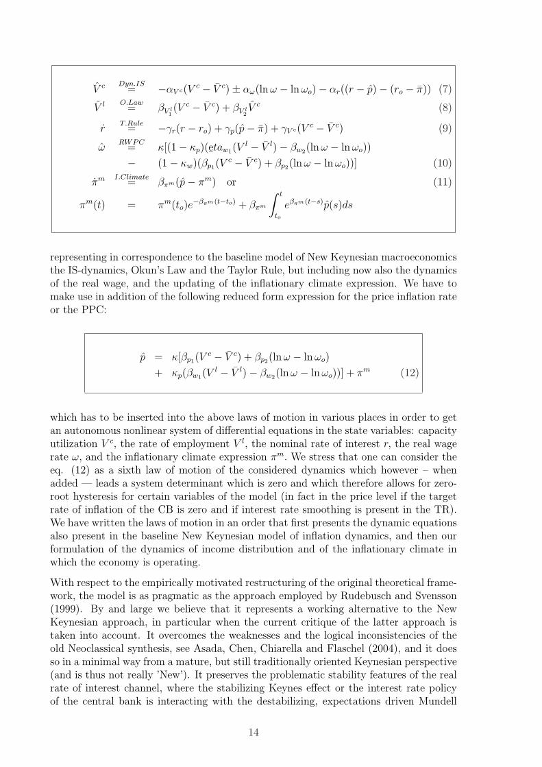
Sketch of proof: We have for the sign structure in this Jacobian under the givenassumptions the following situation to start with (we here assume as limiting situationγr = 0 and have already simplified the law of motion for V l by means of the one forV c through row operations that are irrelevant for the size of the determinant to becalculated):

J =

± + − ± ++ 0 0 0 0+ + 0 + +− + 0 − 0+ + 0 + 0

.

We note that the ambiguous sigh in the entry J11 in the above matrix is due to the factthat the real rate of interest is a decreasing function of the inflation rate which in turndepends positively on current rates of capacity utilization.

Using the second row and the last row in their dependence on the partial derivatives ofp we can reduces this Jacobian to

J =

0 0 − ± ++ 0 0 0 00 0 0 0 +0 + 0 − 00 + 0 + 0

17

without change in the sign of its determinant. In the same way we can now use thethird row to get another matrix without any change in the sign of the correspondingdeterminants

J =

0 0 − ± 0+ 0 0 0 00 0 0 0 +0 + 0 − 00 + 0 + 0

The last two columns can under the observed circumstances be further reduced to

J =

0 0 − ± 0+ 0 0 0 00 0 0 0 +0 + 0 0 00 0 0 + 0

which finally gives

J =

0 0 − 0 0+ 0 0 0 00 0 0 0 +0 + 0 0 00 0 0 + 0

.

This matrix is easily shown to exhibit a negative determinant which proves the propo-sition, also for all values of γr which are chosen sufficiently small.

Proposition 2:

Assume that the parameters βw2 , βp2 , αω and βπm are all set equal to zero.This decouples the dynamics of V c, V l, r from the rest of the system. Assumefurthermore that the partial derivative of the first law of motion dependsnegatively on V c, i.e., the dynamic multiplier process, characterized by αV c ,dominates this law of motion with respect to the overall impact of the rate ofcapacity utilization V c.10 Then: The interior steady state of the implied 3Ddynamical system

V c = −αV c(V c − V c)− αr((r − p)− (ro − π)) (13)

V l = βV l1(V c − V c) (14)


is locally asymptotically stable if the interest rate smoothing parameter γr

and the employment adjustment parameter βV l are chosen sufficiently smallin addition.

Sketch of proof: In the considered situation we have for the Jacobian of these reduceddynamics at the steady state:

J =

− + −+ 0 0+ + −

10i.e., αV c > αpκκpβw.

18

The determinant of this Jacobian is obviously negative if the parameter γr is chosensufficiently small. Similarly, the sum of the minors of order 2: a2, will be positive if βV l

is chosen sufficiently small. The validity of the full set of Routh-Hurwitz conditions theneasily follows, since trace J = −a1 is obviously negative and since det J is part of theexpressions that characterize the product a1a2.

Proposition 3:

Assume now that the parameter αω is negative, but chosen sufficiently small,while the error correction parameters βw2 , βp2 are still kept at zero. Then:The interior steady state of the resulting 4D dynamical system (where thestate variable ω is now included)

V c = −αV c(V c − V c)− αω(ln ω − ln ωo)− αr((r − p)− (ro − π)) (16)

V l = βV l1(V c − V c) (17)


ω = κ[(1− κp)βw1(Vl − V l)− (1− κw)βp1(V

c − V c) (19)

is locally asymptotically stable.

Sketch of proof: It suffices to show in the considered situation that the determinantof the resulting Jacobian at the steady state is positive, since small variations of theparameter αω must then move the zero eigenvalue of the case αω = 0 into the negativedomain, while leaving the real parts of the other eigenvalues – shown to be negative inthe preceding proposition – negative. The determinant of the Jacobian to be consideredhere – already slightly simplified – is characterized by

J =

0 + − −+ 0 0 00 + − 00 + 0 0

This can be further simplified to

J =

0 0 0 −+ 0 0 00 0 − 00 + 0 0

without change in the sign of the corresponding determinant which proves the proposi-tion.

We note that this proposition also holds where βp2 > βw2κp holds true as long as thethereby resulting real wage effect is weaker than the one originating from αω. Finally –and in sum – we can also state that the full 5D dynamics must also exhibit a locallystable steady state if βπm is made positive, but chosen sufficiently small, since we havealready shown that the full 5D dynamics exhibits a negative determinant of its Jacobianat the steady state under the stated conditions. Increasing βπm from zero to a smallpositive value therefore must mover the corresponding zero eigenvalue into the negativedomain of the plane of complex numbers.

19

Summing up, we can state that a weak Mundell effect, the neglect of Blanchard-Katzerror correction terms, a negative dependence of aggregate demand on real wages, cou-pled with nominal wage and also to some extent price level inertia (in order to allow fordynamic multiplier stability ), a sluggish adjustment of the rate of employment towardsactual capacity utilization and a Taylor rule that stresses inflation targeting thereforeare here (for example) the basic ingredients that allow for the proof of local asymptoticstability of the interior steady state of the dynamics (7) – (11). We expect howeverthat indeed a variety of other and also more general situations of convergent dynamicscan be found, but have to leave this here for future research and numerical simulationsof the model. Instead we now attempt to estimate the signs and also the sizes of theparameters of the model in order to gain insight into the question to what extent forexample the US economy after World War II supports one of the real wage effects con-sidered in figure 1 and also the possibility of overall asymptotic stability for such aneconomy, despite a destabilizing Mundell effect in the real interest rate channel. Due toproposition 1 we know that the dynamics will generally only loose asymptotic stabilityin a cyclical fashion (by way of a Hopf-bifurcation) and will indeed do so if the param-eter βπm is chosen sufficiently large. We thus arrive at a radically different outcome forthe dynamics implied by our mature traditional Keynesian approach as compared tothe New Keynesian dynamics. the next topic naturally here is if the economy can beassumed to be in the convergent regime of its alternative dynamical possibilities. Thisof course can only be decided by an empirical estimation of its various parameters whichis the subject of the now following section.

5 Estimating the model

We now provide some estimates for the signs and sizes of the parameters of the modelof this paper and will do so – with respect to the wage-price spiral – on the level ofits structural form (where it has not yet been reduced to the dynamics of real wages,see eq. (12)). The further aim of these estimates is of course to determine whether theimplied autonomous reduced form 5D dynamics we considered in the preceding section –obtained when equation (12) is inserted into (7) – (11) – exhibits asymptotic stability of(convergence to) its interior steady state position. in its theoretical form these dynamicsexhibit the following sign structure in their Jacobian, calculated at its interior steadystate:

J =

± + − ± +± + − ± ++ + − ± +− + 0 − 0+ + 0 ± 0

.

There are therefore a variety of ambiguous effects embedded in the general form of itsdynamics, due to the Mundell-effect and the Rose-effect in the dynamics of the goods-market, and the opposing Blanchard-Katz error correction terms in the reduced formprice Phillips curve. In section 4 we have then considered certain special cases of thegeneral model which allowed for the derivation of asymptotic stability of the steadystate and its loss of stability by way of Hopf bifurcations if certain speed parametersbecome sufficiently large. In the present section we now provide empirical estimates

20

for the laws of motion (7) – (11) of our disequilibrium AS-AD model, by means ofthe structural form of the wage and price Phillips curve, coupled with the dynamicmultiplier equation, Okun’s law and the interest rate policy rule. These estimates, onthe one hand, serve the purpose of confirming the parameter signs we have specified inthe initial theory-guided formulation of the model and to determine the sizes of theseparameters in addition. On the other hand, we have three different situations where wecannot specify the parameter signs on purely theoretical grounds and where we thereforeaim at obtaining these signs from the empirical estimates of the equations where thishappens.

There is first of all, see eq. (7), the ambiguous influence of real wages on (the dynamicsof) the rate of capacity utilization, which should be a negative one if investment is moreresponsive than consumption to real wage changes and a positive one in the opposite case.There is secondly, with an immediate impact effect if the rates of capacity utilization forcapital and labor are perfectly synchronized, the fact that real wages rise with economicactivity through money wage changes on the labor market, while they fall with it throughprice level changes on the goods market, see eq. (9). Finally, we have in the reducedform equation for price inflation a further ambiguous effect of real wage increases, whichthere lower p through their effect on wage inflation, while speeding up p through theireffect on price inflation, effects which work into opposite directions in the reduced formprice PC (12). Mundell-type, Rose-type and Blanchard-Katz error-correction feedbackchannels therefore make the dynamics indeterminate on the general level.

In all of these three cases empirical analysis will now indeed provide us with definiteanswers which ones of these opposing forces will be the dominant ones. Furthermore,we shall also see that the Blanchard and Katz (2000) error correction terms do play arole in the US-economy, in contrast to what has been found out by these authors for themoney wage PC in the U.S. However, we will not attempt to estimate the parameterβπm that characterizes the evolution of the inflationary climate in our economy. Instead,we will use moving averages with linearly declining weights for its representation, whichallows to bypass the estimation of the law of motion (11). We consider this as thesimplest approach to the treatment of our climate expression (comparable with recentNew Keynesian treatments of hybrid expectation formation), which should later on bereplaced by more sophisticated ones, for example one that makes use of the Livingstonindex for inflationary expectations as in Laxton et al. (2000) which in our view mirrorssome adaptive mechanism in the adjustment of inflationary expectations.

We take an encompassing approach to conduct our estimates. The structural laws ofmotion of our economy, see section 3, have been formulated in an intrinsically nonlinearway (due to certain growth rate formulations). We note that single equations estimateshave suggested to only use αV l

2in the equation that describes the dynamics of the

employment rate. We use moreover both the logs of real wages and unit-wage costs (indetrended form) in the equation describing goods market dynamics, in an attempt toestimate separately the influence of income distribution on aggregate demand as inducedvia consumption (a positive one) and via investment (a negative one).11 In the wage-price spiral we use however – in line with Blanchard and Katz (2000) – the log of unitwage costs throughout, again removing their significant downward trend in the employeddata appropriately.

11Using a single measure for the influence of income distribution on aggregate demand basicallyaggregates the separated outcome as we shall see our further estimates below.

21

We do this in conjunction with time-invariant estimates of all the parameters of ourmodel. This in particular implies that Keynes’ (1936) explanation of the trade cycle,which employed systematic changes in the propensity to consume, the marginal efficiencyof investment and liquidity preference over the course of the cycle, find no applicationhere and that – due the use of detrended measures for income distribution changes andunit-wage costs – also the role of technical change is downplayed to a significant degree,in line with its neglect in the theoretical equations of the model presented in section 3. Asa result we expect to obtain from our estimates long-phased economic fluctuations, butnot long -waves yet, since important fluctuations in aggregate demand (based on time-varying parameters) are still ignored and since the dynamics is then driven primarily byslowly changing income distribution, indeed a slow process in the overall evolution ofthe U.S. economy after world war II.

To show that such an understanding of the model is a suitable description of (some of)the dynamics of the observed data, we first fit a corresponding 6D VAR model to thedata to find out the dynamics in the six independent variables there employed. We thenidentify a linear structural model that parsimoniously encompasses the employed VAR.Finally, we contrast our nonlinear structural model, i.e., the laws of motion (1) to (5)in structural form, with the linear structural VAR model and show through a J Testthat the nonlinear model is indeed preferred by the data. In this way we show that ournonlinear structural model represents a proper description of the data.

The relevant variables for the following investigation are the wage inflation rate, the priceinflation rate, the rates of utilization of labor and of capital, the nominal interest rate,the log of the real wage and / or of average unit wage cost, to be denoted in the followingby: d ln wt, d ln pt, V

lt , V c

t , rt, rwt, and uct, where uct(rwt) is the cycle component of thelog of the time series for the unit real wage cost (the real wage), both filtered by thebandpass filter.12

5.1 Data Description

The empirical data of the corresponding time series are taken from the Federal ReserveBank of St. Louis data set (see http:/www.stls.frb.org/fred). The data are quarterly ,seasonally adjusted and are all available from 1948:1 to 2001:2. Except for the unem-ployment rates of the factors labor, U l, and capital, U c, the log of the series are used(see table 1).

12For details of bp filter see Baxter and King (1991).

22

dlnw

1947 1953 1959 1965 1971 1977 1983 1989 1995-0.014

-0.007

0.000

0.007

0.014

0.021

0.028

0.035dlnwp

1947 1953 1959 1965 1971 1977 1983 1989 1995-0.02

-0.01

0.00

0.01

0.02

0.03

0.04

lnVl

1948 1954 1960 1966 1972 1978 1984 1990 1996-0.125

-0.100

-0.075

-0.050

-0.025lnVc

1948 1954 1960 1966 1972 1978 1984 1990 1996-0.40

-0.35

-0.30

-0.25

-0.20

-0.15

-0.10

-0.05

lnrw

1954 1959 1964 1969 1974 1979 1984 1989 1994 1999-0.020

-0.015

-0.010

-0.005

0.000

0.005

0.010

0.015

0.020lnuc

1950 1956 1962 1968 1974 1980 1986 1992 1998-0.024

-0.012

0.000

0.012

0.024

0.036

Pi

1950 1956 1962 1968 1974 1980 1986 1992 19980.000

0.005

0.010

0.015

0.020

0.025r

1955 1960 1965 1970 1975 1980 1985 1990 1995 20000.00

0.02

0.04

0.06

0.08

0.10

0.12

0.14

0.16

0.18

Figure 2: The fundamental data of the model.

23

Variable Transformation Mnemonic Description of the untransformed seriesU l = 1− V l UNRATE/100 UNRATE Unemployment RateU c = 1− V c 1-CUMFG/100 CUMFG Capacity Utilization: Manufacturing,

Percent of Capacityln w ln(COMPNFB) COMPNFB Nonfarm Business Sector: Compensa-

tion Per Hour, 1992=100ln p ln(GNPDEF) GNPDEF Gross National Product: Implicit Price

Deflator, 1992=100ln yn = ln y − ln ld ln(OPHNFB) OPHNFB Nonfarm Business Sector; Output Per

Hour of All Persons, 1992=100UC = ln w − ln p− ln yn ln

(COMPRNFB

OPHNFB

)COMPRNFB Nonfarm Business Sector: Real Com-

pensation Per Output Unit, 1992=100RW = ln w − ln p ———- ——— log of the real wager ———- ——— Federal Funds Rate

Table 1: Data used for the empirical investigation

Note that we now use ln wt and ln pt, i.e., logarithms, in the place of the original levelmagnitudes. Their first differences d ln wt, d ln pt thus give the current rate of wage andprice inflation. We use πt in this section to denote here specifically a moving averageof price inflation with linearly decreasing weights over the past 12 quarters, interpretedas a particularly simple measure for the inflationary climate expression of our model,and we denote by V l, V c(U l, U c) the rates of (under-)utilization of labor and the capitalstock. The graphs of the time series of these variables are shown in the figure 2.

There is a pronounced downward trend in part of the employment rate series (over the1970’s and part of the 1980’s) and in the wage share (normalized to 0 in 1996). Thelatter is not the topic of this paper and will only briefly be considered in the concludingsection. Wage inflation shows three to four trend reversals, while the inflation climaterepresentation clearly show two periods of low inflation regimes and in between a highinflation regime.

We expect that the 6 independent time series for wages, prices, capacity utilization rates,labor productivity and the interest rate (federal funds rate) are stationary. The graphsof the series for wage and price inflation, capacity utilization rates and labor productivitygrowth, d ln wt, d ln pt, V

lt , V c

t , d ln ynt confirm our expectation. In addition we carry outthe DF unit root test for each series. The test results are shown in table 2.

Variable Sample Critical Value Test Statisticd ln w 1947:02 TO 2000:04 -3.41000 -3.74323d ln p 1947:02 TO 2000:04 -3.41000 -3.52360lnV l 1948:02 TO 2000:04 -1.95000 -0.75474lnV c 1948:02 TO 2000:04 -3.41000 -4.15536

r 1955:01 TO 2000:04 -1.95000 -0.94144lnuc 1950:01 TO 2000:04 -3.41000 -7.09932

Table 2: Summary of DF-Test Results

The applied unit root test confirms our expectations with the exception of V l and r.Although the test cannot reject the null of unit root, there is no reason to expect therate of unemployment and the federal funds rate as being unit root processes. Indeed weexpect that they are constrained in certain limited ranges, say from zero to 0.3. Due to

24

the lower power of the DF test, this test result should only provide hints that the rate ofunemployment and the federal funds rate exhibit strong autocorrelations, respectively.

5.2 Estimation of the unrestricted VAR

Given the assumption of stationarity, we can construct a VAR model for these 6 variablesto mimic the DGP of these 6 variables by linearizing our given structural model in anobvious way.

d ln wt

d ln pt

ln V lt

ln V ct

rt

uct

=

c1

c2

c3

c4

c5

c6

+

b1

b2

b3

b4

b5

b6

d74+P∑

k=1

a11k a12k a13k a14k a15k a16k






d ln wt−k

d ln pt−k

ln V lt−k

ln V ct−k

rt−k

uct−k

+

e1t

e2t

e3t

e4t

e5t

(20)

To determine the lag length of the VAR we apply sequential likelihood tests. We startwith a lag length of 24, at which the residuals can be taken as a WN process. Thesequence likelihood ratio test procedure gives a lag length of 11. The test results arelisted below.

• H0 : P = 20 v.s. H1 : P = 24Chi-Squared(144)= 147.13 with Significance Level 0.91





According to these test results we use a VAR(12) model to represent a general modelthat should be a good approximation of the DGP. Because the variable uct is treatedas exogenous in the structural form (1) – (6) of the dynamic system , we factorize theVAR(12) process into a conditional process of d ln wt, d ln pt, ln V l

t , ln V ct , rt given uct and

the lagged variables, and the marginal process of uct given the lagged variables:

25

d ln wt

d ln pt

ln V lt

ln V ct

rt

=

c∗1c∗2c∗3c∗4c∗5

+

b∗1b∗2b∗3b∗4b∗5

d74 +

a1

a2

a3

a4

a5

uct (21)

+P∑

k=1

a∗11k a∗12k a∗13k a∗14k a∗15k a∗16k

a∗21k a∗22k a∗23k a∗24k a∗25k a∗26k

a∗31k a∗32k a∗33k a∗34k a∗35k a∗36k

a∗41k a∗42k a∗43k a∗44k a∗45k a∗46k

a∗51k a∗52k a∗53k a∗54k a∗55k a∗56k

d ln wt−k

d ln pt−k

ln V lt−k

ln V ct−k

rt−k

uct−k

+

e∗1t

e∗2t

e∗3t

e∗4t

e∗5t

uct = c6 +P∑

k=1

(a61k a62k a63k a64k a65k a66k

)

d ln wt−k

d ln pt−k

ln V lt−k

ln V ct−k

rt−k

uct−k

+ e6t (22)

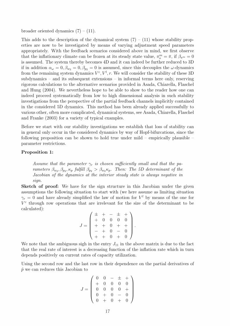
We now examine whether uct can be taken as ”exogenous” variable. The partial sys-tem (21) is exactly identified. Hence the variables uct are weakly exogenous for theparameters in the partial system.13 For the strong exogeneity of uct, we test whetherd ln wt, d ln pt, ln V l

t , ln V ct , rt Granger cause uct. The test is carried out by testing the

hypothesis: H0 : aijk = 0, (i = 6; j = 1, 2, 3, 4, 5; k = 1, 2, ..., 12) in (22) based on thelikelihood ratio

• Chi-Squared(60)=57.714092 with Significance Level 0.55972955

The result of the test is uct is strongly exogenous with respect to the parameters in (21).Hence we can investigate the partial system (21) taking uct as exogenous.

5.3 Estimation of the Structural Model

As discussed in section 3, the law of motion for the real wage rate, eq. (10), represents areduced form expression for the two structural equations for d ln wt and d ln pt. Notingagain that the inflation climate variable is defined here as a linearly declining function ofpast price inflation rates, the dynamics of the system (1) – (6) is equivalently presented

13For a detailed discussion of this procedure, see Chen (2003).

26

by the following equations:14

d ln wt = βw1 ln V lt−1 − βw2uct−1 + κwd ln pt + (1− κw)πt + c1 + e1t (23)

d ln pt = βp1 ln V ct−1 + βp2uct−1 + κpd ln wt + (1− κp)πt + c2 + e2t (24)

d ln V lt = αV l

2d ln V l

t + e3t (25)

d ln V ct = −αV c ln V c

t−1 − αr(rt−1 − d ln pt)− αωuct−1 + c4 + e4t (26)

drt = −γrrt−1 + γpd ln pt + γV c ln V ct−1 + c5 + e5t (27)

Obviously, the model (23) – (27) is nested in the VAR(12) of (21). Therefore we can use(21) to evaluate the empirical relevance of the model (23) – (27). First we test whetherthe parameter restrictions on (21) implied by (23) – (27) are valid.

The linearized structural model (23) – (27) puts 349 restrictions on the unconstrainedVAR(12) of the system (21). Applying likelihood ratio methods we can test the validityof these restrictions. For the period from 1965:1 to 2000:4 we cannot reject the null ofthese restrictions. The test result is the following:

• Chi-Squared(349)= 361.716689 with Significance Level 0.34902017

Obviously, the specification (23) – (27) is a valid one for the data set from 1965:1 to2000:4. This result shows strong empirical relevance for the laws of motions as describedin (1) – (6) as a model for the U.S. economy from 1965:1 to 2000:4. It is worthwhileto note that altogether 349 restrictions are implied through the structural form of thesystem (1) – (6) on the VAR(12) model. A p-value of 0.39 thus means that (1) – (6)is a much more parsimonious presentation of the DGP than VAR(12), and henceforth amuch more efficient model to describe the economic dynamics for this period.

To get a result that is easier to interpret from the economic perspective, we transform themodel (23) – (27) back to its originally nonlinear form (1) – (6), now using in addition atfirst two distributional variables to measure the influence of consumption and investmenton aggregate demand:15

d ln wt = βw1Vlt−1 − βw2uct−1 + κwd ln pt + (1− κw)πt + c1 + e1t (28)

d ln pt = βp1Vct−1 + βp2uct−1 + κpd ln wt + (1− κp)πt + c2 + e2t (29)

d ln V lt = αV l

2d ln V c

t + e3t (30)

d ln V ct = −αV cV c

t−1 + αωrwt−1 − αuuct−1 − αr(rt−1 − d ln pt) + c4 + e4t (31)

drt = −γrrt−1 + γpd ln pt + γV cV ct−1 + c5 + e5t (32)

The estimation results for this particular case are listed in the appendix to this paper.They do not differ in their qualitative implications from the estimates to be consideredbelow where only the measure uc is used to consider the role of income distribution

14Note here that the difference operator d is to be interpreted as backward in orientation and thatthe nominal rate of interest is dated at the beginning of the relevant period. The linearly decliningmoving average πt in turn concerns the past twelve price inflation rates.

15Note that drt = −γrrt−1 + γpd ln pt + γV cV ct−1 + c5 + e5t can also be represented by rt = (1 −

γr)rt−1 + ... in the equations to be estimated below.

27

in the dynamic multiplier equation and where the Taylor rule is represented by rt =(1− γr)rt−1 + ...

This model therefore differs from the model (23) – (27) by referring now again to theexplaining variables V c and V l instead of ln V c and ln V l which were necessary to con-struct a linear VAR(12) system. In addition we have considered the log of the real wagerw as an explaining variable to account for the influence of consumption demand on therate of capacity utilization and the log of average unit wage costs uc as the explainingvariable for the profitability effect on investment behavior. We compare on this basisthe model (28) – (32) with the model (23) – (27) in a nonnested testing framework. Ap-plying the J test to such a nonlinear estimation procedure, we get significant evidencethat the model (28) – (32) is to be preferred to the model (23) – (27).

Model J testH1 : Model of (23) – (27) is true tα = 4.611H2 : Model of (28) – (32) is true tφ = −0.928

We have already omitted in the following summary of our model estimate the insignif-icant parameters in the shown quantitative representation of the structural model andalso the stochastic terms. By putting furthermore the NAIRU expressions and all otherexpressions that are here still assumed as constant into overall constant terms, we there-fore finally get following estimation result:16

d ln wt = 0.11V lt−1 − 0.09uct−1 + 0.62d ln pt + 0.38πt − 0.10 (33)

d ln pt = 0.03V ct−1 + 0.07uct−1 + 0.34d ln wt + 0.66πt − 0.03 (34)

d ln V lt = 0.20d ln V c

t (35)

d ln V ct = −0.11V c

t−1 − 0.17(rt−1 − d ln pt) + 0.48rwt−1 − 0.80uct−1 + 0.10 (36)

drt = −0.10rt−1 + 0.43d ln pt + 0.05V ct−1 − 0.03 (37)

If one disregards the possibly questionable application of both the real wage and theaverage unit wage costs as explaining variables in the equation driving goods marketdynamics, employing the single measure uc in their place, one gets as approximateparameter values (with basically the same statistical characteristics):




t (40)


t−1 − 0.17(rt−1 − d ln pt)− 0.74uct−1 + 0.08 (41)

rt = 0.90rt−1 + 0.41d ln pt + 0.05V ct−1 − 0.04 (42)

Next we compare the preceding situation with the case where the climate expression πis based on 24 quarter horizon in the place of the 12 quarter horizon we have employedso far.

16We have here reduced the weights in the cost pressure expressions slightly in order to meet the unityrestrictions on these weights that are postulated by theory and thus here only represent the degree offorward-looking behavior in a somewhat stylized from, see the appendix to this paper for the exactresults and their evaluation by means of t-statistics, R2 terms and Durbin-Watson coefficients.

28

d ln wt = 0.13V lt−1 − 0.08uct−1 + 0.69d ln pt + 0.31π24t − 0.12 (43)

d ln pt = 0.03V ct−1 + 0.09uct−1 + 0.50d ln wt + 0.50π24t − 0.03 (44)


t (45)


t−1 − 0.17(rt−1 − d ln pt)− 0.74uct−1 + 0.09 (46)

rt = 0.90rt−1 + 0.43d ln pt + 0.05V ct−1 − 0.03 (47)

We see that the application of a time horizon of 24 quarters for the formation of theinflationary climate variable does not alter the qualitative properties of the dynamicssignificantly as compared to the case of a moving average with linearly declining weightsover 12 quarters only (which approximately corresponds to a value of βπm = 0.15 inan adaptive expectations mechanism as used for the theoretical version of the model insection 3). Even choosing only a six quarter horizon for our linearly declining weightspreserves the qualitative features of our estimated model and also by and large the stabil-ity properties of the dynamics as we shall see later on, though inflationary expectationsover the medium run are then updated with a speed comparable to the ones used inhybrid New Keynesian approaches to their price PC:

d ln wt = 0.11V lt−1 − 0.10uct−1 + 0.40d ln pt + 0.60π6t − 0.10 (48)

d ln pt = 0.03V ct−1 + 0.03uct−1 + 0.18d ln wt + 0.82π6t − 0.02 (49)


t (50)


t−1 − 0.17(rt−1 − d ln pt)− 0.74uct−1 + 0.08 (51)

rt = 0.90rt−1 + 0.44d ln pt + 0.05V ct−1 − 0.04 (52)

We thereby arrive at the general qualitative result that wages are more flexible thanprices with respect to their corresponding measures of demand pressure and that wageearners are more short-sighted than firms with respect to the weight they give theircurrent (perfectly foreseen) measure of cost pressure as compared to the inflationaryclimate that surrounds this situation. Blanchard and Katz (2000) type error correctionmechanisms play a role both in the WPC and also in the PPC for the U.S. economyand have the sign that is predicted by theory, in contrast to what is found out bythese two authors. We have the validity of Okun’s law with an elasticity coefficient ofaround 20 percent and have the correct signs for the dynamic multiplier process as wellas with respect to the influence of changing real rate of interests on economic activity.Finally, the impact of income distribution on the change in capacity utilization is (insum) a negative one and thus of an orthodox type, meaning that rising average unitwage costs will decrease economic activity, and will therefore imply at least from apartial perspective that increasing wage flexibility is stabilizing, while increasing priceflexibility (again with respect to its measure of demand pressure) is not. We note, finally,that the different definitions of the inflationary climate used in these system estimatesprimarily and not unexpectedly changes the weights in the employed cost pressure terms,while it leaves intact the qualitative nature of all other parameter estimates.

We conclude from the above that it should be legitimate to use (38) – (42) for the furtherevaluation of the dynamic properties of our theoretical model of section 3, in order to

29

see what more can be obtained as compared to the theoretical results of section 4 whenempirically supported parameter sizes are approximately taken into account. To makethis approximation a sensible procedure we finally also report single equations estimatesfor our 5D system in order to get a feeling for the intervals in which the parameter valuesmay sensibly assumed to be in.




t (55)


t−1 − 0.18(rt−1 − d ln pt)− 0.79uct−1 + 0.12 (56)

rt = 0.90rt−1 + 0.44d ln pt + 0.05V ct−1 − 0.03 (57)

Again the weights concerning the cost pressure items are changed significantly and alsocertain speeds of adjustment. We do not expect however that this changes the stabilityproperties of the dynamics in a qualitative sense and have to check this in the followingsections from the theoretical as well as numerical perspective.

The above by and large similar representation of the signs and the sizes of the parametervalues of our dynamics thus reveal various interesting assertions on the relative impor-tance of demand pressure influences as well as cost pressure effects in the wage-pricespiral of the U.S. economy. The Blanchard and Katz error correction terms have thecorrect signs and are of relevance in general. Okun’s law holds as a level relationshipbetween the capacity utilization rate and the rate of employment, basically of the formV l/V l = (V c/V c)b with an elasticity parameter b of about 20 percent. The dynamicIS equation shows the from the partial perspective the stabilizing role of the multiplierprocess and a significant dependence of the rate of change of capacity utilization on thecurrent real rate of interest. There is a significant and positive effect of real wages –we conjecture: via consumption – on the growth in activity levels and an even strongernegative effect of real unit wage costs – we conjecture: via investment – on this growthrate of capacity utilization, which in aggregated form however gives that the economy isprofit-led as far as aggregate goods demand is concerned, i.e., real wage cost increasessignificantly decrease economy activity.

Finally, for the Taylor interest rate policy rule, we get the result that interest ratesmoothing takes place around the ten percent level, that monetary policy is to be con-sidered as passive (γp = 0.43) in such an environment as far as the inflation gap isconcerned, and that there is only a weak direct influence of the output gap on the rateof change of the nominal rate of interest. We stress here that this result will change con-siderably if interest rate smoothing is removed from the model which however impliesin our modelling framework that the steady state rate of interest is no longer uniquelydetermined. Finally, turning back to the case of interest rate smoothing, it is not possi-ble to recover the steady state rate of interest from the constant in the above estimatedTaylor rules in a statistically significant way, since the expression implied for this rateby our formulation of the Taylor rule would be:

ro = (const + γpπ + γV c)/γr

which does not determine this rate with any reliable statistical confidence. This also

30

holds for the other constants that we have assumed as given in our formulation ofKeynesian DAS-DAD dynamics.

In sum we therefore get that the system estimates of this section provides us with a resultthat confirms theoretical sign restrictions. It moreover provides by and large definiteanswers with respect to the role of income distribution in the considered disequilibriumAS-AD or DAS-DAD dynamics, confirming in particular the orthodox point of view thateconomic activity is – in sum – likely to depend negatively on real wage or unit wage costs.We have also a negative real wage effect in the dynamics of income distribution, in thesense that the growth rate of real wages, see our reduced form real wage dynamics (??),depends – through Blanchard and Katz error correction terms – negatively on the realwage. Its dependence on economic activity levels however is somewhat ambiguous, butin any case small. Real wages – possibly – therefore only weakly increase with increasesin the rate of capacity utilization which in turn however depends in an unambiguous waynegatively on the real wage, implying in sum that the Rose (1967) real wage channel isthere, but not dominating the dynamic outcomes.

Finally, the estimated adjustment speed of the price level is so small that the dynamicmultiplier effect dominates the overall outcome of changes in capacity utilization onthe growth rate of this utilization rate, which therefore establishes a further stabilizingmechanism in the reduced form of our multiplier equation. The model and its estimatesthus by and large confirm the conventional Keynesian view on the working of the econ-omy and thus provide in sum a result very much in line with the traditional ways ofreasonings from a Keynesian perspective, with one important qualification however, aswe will show in the next sections, namely that downward money wage flexibility is goodfor economic stability, in line with Rose’s (1967) model of the employment cycle, but inopposition to what Keynes (1936) stated on the role of rigid money wages. Yet, the roleof income distribution in aggregate demand and wage vs. price flexibility was not reallya topic in the General Theory, which therefore did not comment on the possibility thatwage declines may lead the economy out of a depression via a channel different from theconventional now so-called Keynes-effect.

6 Stability analysis of the estimated model

In the preceding section we have provided definite answers with respect to the type ofreal wage effect present in the data of the U.S. economy after World War II, concerningthe dependence of aggregate demand on the real wage, the degrees of wage and priceflexibilities and the degree of forward-looking behavior in the wage and price PC. Theresulting combination of effects and the estimated sizes of the parameters (in particularthe relative degree of wage vs. price flexibility) suggest that their particular type ofinteraction is favorable for stability. We stress however that the inflation climate is sofar only measured by a moving average of past inflation rates with linearly decliningweights. The role of a varying parameter βπm – which when increased will definitelydestabilize the economy – is thus not yet considered at present.

We start the stability analysis of the model with estimated parameters from the followingreference situation (the system estimate where the inflationary climate is measured as

31

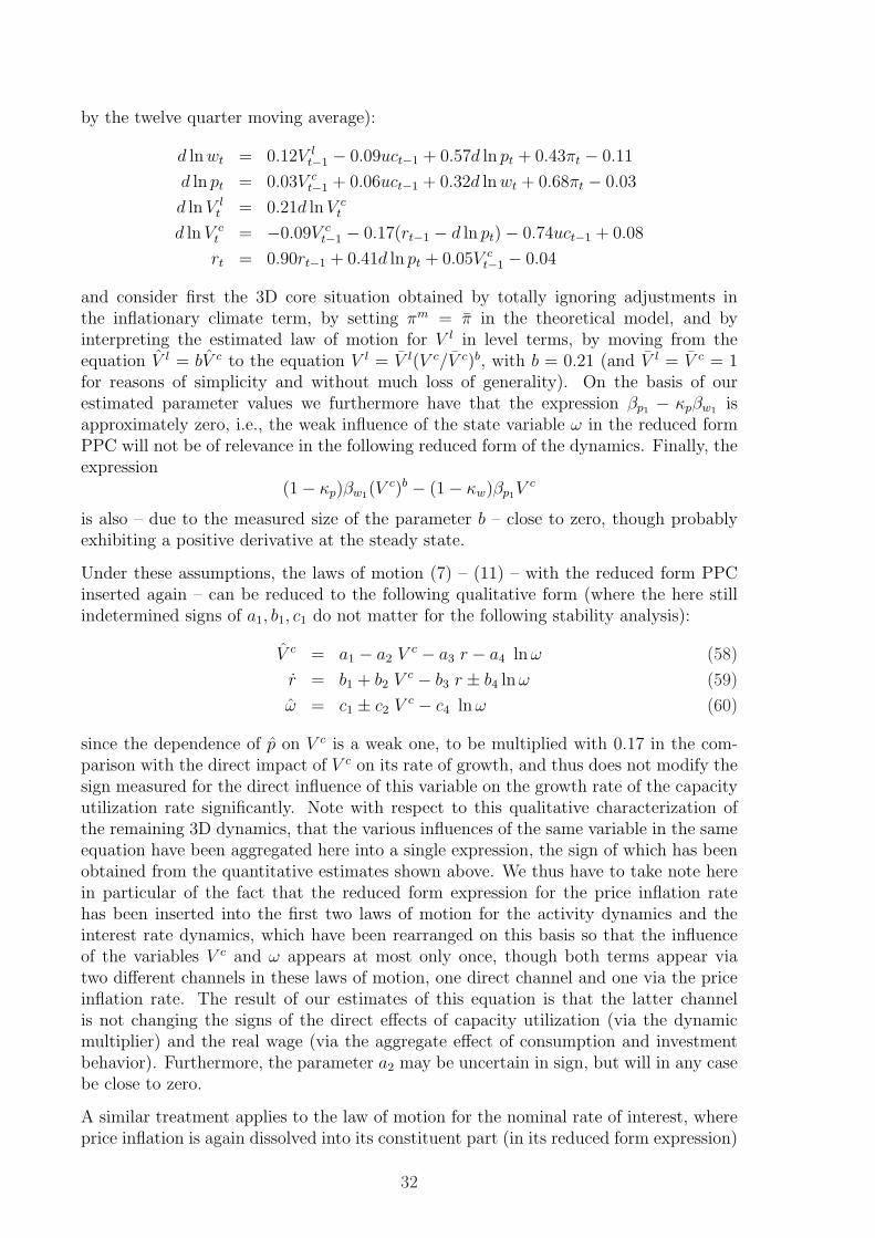
by the twelve quarter moving average):

d ln wt = 0.12V lt−1 − 0.09uct−1 + 0.57d ln pt + 0.43πt − 0.11

d ln pt = 0.03V ct−1 + 0.06uct−1 + 0.32d ln wt + 0.68πt − 0.03


t


t−1 − 0.17(rt−1 − d ln pt)− 0.74uct−1 + 0.08

rt = 0.90rt−1 + 0.41d ln pt + 0.05V ct−1 − 0.04

and consider first the 3D core situation obtained by totally ignoring adjustments inthe inflationary climate term, by setting πm = π in the theoretical model, and byinterpreting the estimated law of motion for V l in level terms, by moving from theequation V l = bV c to the equation V l = V l(V c/V c)b, with b = 0.21 (and V l = V c = 1for reasons of simplicity and without much loss of generality). On the basis of ourestimated parameter values we furthermore have that the expression βp1 − κpβw1 isapproximately zero, i.e., the weak influence of the state variable ω in the reduced formPPC will not be of relevance in the following reduced form of the dynamics. Finally, theexpression

(1− κp)βw1(Vc)b − (1− κw)βp1V

c

is also – due to the measured size of the parameter b – close to zero, though probablyexhibiting a positive derivative at the steady state.

Under these assumptions, the laws of motion (7) – (11) – with the reduced form PPCinserted again – can be reduced to the following qualitative form (where the here stillindetermined signs of a1, b1, c1 do not matter for the following stability analysis):

V c = a1 − a2 V c − a3 r − a4 ln ω (58)

r = b1 + b2 V c − b3 r ± b4 ln ω (59)

ω = c1 ± c2 V c − c4 ln ω (60)

since the dependence of p on V c is a weak one, to be multiplied with 0.17 in the com-parison with the direct impact of V c on its rate of growth, and thus does not modify thesign measured for the direct influence of this variable on the growth rate of the capacityutilization rate significantly. Note with respect to this qualitative characterization ofthe remaining 3D dynamics, that the various influences of the same variable in the sameequation have been aggregated here into a single expression, the sign of which has beenobtained from the quantitative estimates shown above. We thus have to take note herein particular of the fact that the reduced form expression for the price inflation ratehas been inserted into the first two laws of motion for the activity dynamics and theinterest rate dynamics, which have been rearranged on this basis so that the influenceof the variables V c and ω appears at most only once, though both terms appear viatwo different channels in these laws of motion, one direct channel and one via the priceinflation rate. The result of our estimates of this equation is that the latter channelis not changing the signs of the direct effects of capacity utilization (via the dynamicmultiplier) and the real wage (via the aggregate effect of consumption and investmentbehavior). Furthermore, the parameter a2 may be uncertain in sign, but will in any casebe close to zero.

A similar treatment applies to the law of motion for the nominal rate of interest, whereprice inflation is again dissolved into its constituent part (in its reduced form expression)

32

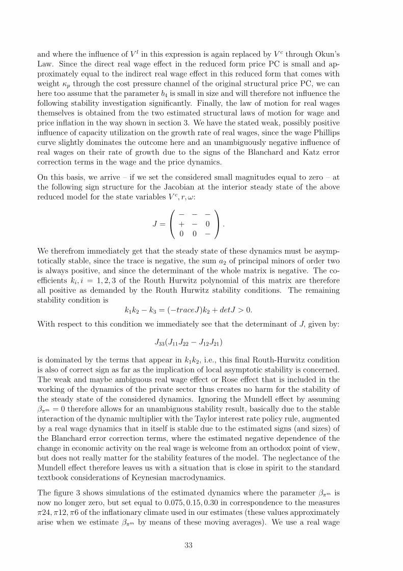
and where the influence of V l in this expression is again replaced by V c through Okun’sLaw. Since the direct real wage effect in the reduced form price PC is small and ap-proximately equal to the indirect real wage effect in this reduced form that comes withweight κp through the cost pressure channel of the original structural price PC, we canhere too assume that the parameter b4 is small in size and will therefore not influence thefollowing stability investigation significantly. Finally, the law of motion for real wagesthemselves is obtained from the two estimated structural laws of motion for wage andprice inflation in the way shown in section 3. We have the stated weak, possibly positiveinfluence of capacity utilization on the growth rate of real wages, since the wage Phillipscurve slightly dominates the outcome here and an unambiguously negative influence ofreal wages on their rate of growth due to the signs of the Blanchard and Katz errorcorrection terms in the wage and the price dynamics.

On this basis, we arrive – if we set the considered small magnitudes equal to zero – atthe following sign structure for the Jacobian at the interior steady state of the abovereduced model for the state variables V c, r, ω:

J =

− − −+ − 00 0 −

.

We therefrom immediately get that the steady state of these dynamics must be asymp-totically stable, since the trace is negative, the sum a2 of principal minors of order twois always positive, and since the determinant of the whole matrix is negative. The co-efficients ki, i = 1, 2, 3 of the Routh Hurwitz polynomial of this matrix are thereforeall positive as demanded by the Routh Hurwitz stability conditions. The remainingstability condition is

k1k2 − k3 = (−traceJ)k2 + detJ > 0.

With respect to this condition we immediately see that the determinant of J, given by:

J33(J11J22 − J12J21)

is dominated by the terms that appear in k1k2, i.e., this final Routh-Hurwitz conditionis also of correct sign as far as the implication of local asymptotic stability is concerned.The weak and maybe ambiguous real wage effect or Rose effect that is included in theworking of the dynamics of the private sector thus creates no harm for the stability ofthe steady state of the considered dynamics. Ignoring the Mundell effect by assumingβπm = 0 therefore allows for an unambiguous stability result, basically due to the stableinteraction of the dynamic multiplier with the Taylor interest rate policy rule, augmentedby a real wage dynamics that in itself is stable due to the estimated signs (and sizes) ofthe Blanchard error correction terms, where the estimated negative dependence of thechange in economic activity on the real wage is welcome from an orthodox point of view,but does not really matter for the stability features of the model. The neglectance of theMundell effect therefore leaves us with a situation that is close in spirit to the standardtextbook considerations of Keynesian macrodynamics.

The figure 3 shows simulations of the estimated dynamics where the parameter βπm isnow no longer zero, but set equal to 0.075, 0.15, 0.30 in correspondence to the measuresπ24, π12, π6 of the inflationary climate used in our estimates (these values approximatelyarise when we estimate βπm by means of these moving averages). We use a real wage

33

shock (increase by ten percent) to investigate the response of the dynamics to such ashock. The obtained impulse-responses are very similar to each other, also in the casewhere we use π12 in combination with the single equation estimates of our parametervalues. In the considered range for the parameter βπm the responses of the dynamicsare by and large of the shown type, i.e., the system has strong, though cyclical stabilityproperties over this whole range, independently of the particular combination of thespeed of adjustment of the inflationary climate and the set of other parameter values wehave estimated in the preceding section.

We note that the system is subject to zero root hysteresis, since the laws of motionfor V l, V c are here linearly dependent (since αV l

1), has been estimated as being zero),

i.e., it need not converge back to the initially given steady state value of the rate ofcapacity utilization which was assumed to be 1. Note also that the parameter estimatesare based on quarterly data, i.e., the plots in figure 3 correspond to 25 years and thusshow a long period of adjustment, due to the fact that all parameters have been assumedas time invariant so that only the slow process of changing income distribution and itsimplications for Keynesian aggregate demand is driving the economy.

Next we test the stability properties of the model if one of its parameters is varied insize. We find (also for parameter variations that are not shown) that all partial feedbackchains (including the working of the Blanchard / Katz error correction terms) translatethemselves into corresponding ’normal’ eigenvalue reaction patterns for the full 5D dy-namics, with the exception of the speed parameter βw1 where the eigenvalue diagramshows that increasing wage flexibility may become destabilizing if made sufficiently large.This shows that are partial insight may be misleading due to the fact that the corre-sponding feedback chain is only a small component of the many minors that have to beinvestigated in the application of the Routh-Hurwitz conditions to the full 4D dynamics(where Okun’s law is applied in level form).

34

12dfp s12dfp

6dfp

24dfp

cV

100t q=

The maximum real part of eigenvalues is always negative,but there is one pair of conjugate complex eigenvalues

0.075mπβ =

1,2im λ

0.30mπβ =

Figure 2: Responses to real wage shocks in the range of estimated parameter values.

Increasing price flexibility is destabilizing via the Mundell-effect, since the growth rateV c of economic activity can thereby be made to depend positively on its level (via thisreal rate of interest channel, see eq. (12)), leading to an unstable augmented dynamicmultiplier process in the trace of J under such circumstances. Furthermore, such in-creasing price flexibility will give rise to a negative dependence of the growth rate ofthe real wage on economic activity (whose rate of change in turn depends negatively onthe real wage) and thus lead to further sign changes in the Jacobian J. Increasing priceflexibility is therefore bad for the stability of the considered dynamics from at least twoperspectives.

The destabilizing role of price flexibility is enhanced if we add to the above stabilityanalysis for the 3D Jacobian the law of motion for the inflationary climate surroundingthe current evolution of price inflation. Under this extension we go back to a 4D dy-namical system, the Jacobian J of which is obtained by augmenting the previous one inits sign structure in the following way (see again eq. (12))):

J =

− − − ++ − 0 +0 0 − 0+ 0 0 0

.

35

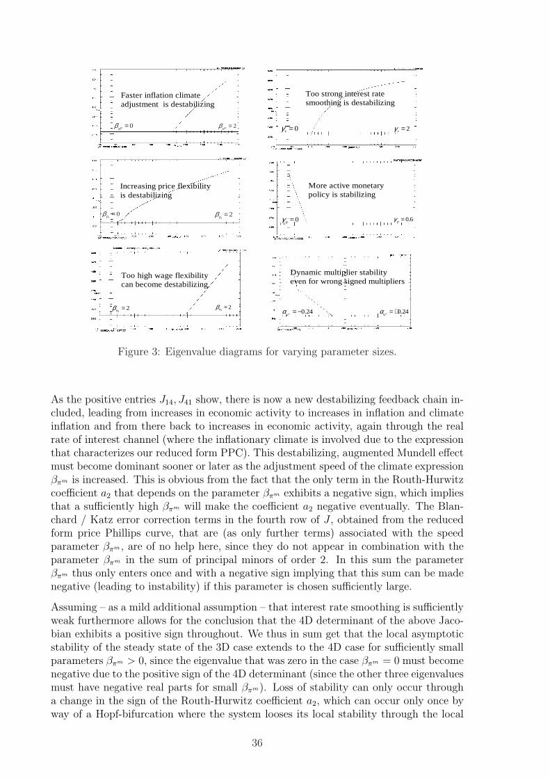
0mπβ = 2mπβ =-

10pβ =

12pβ =

12wβ = 1

2wβ =

2rγ =0rγ =

0pγ = 0.6pγ =

0.24cVα = − 0.24cV

α = +

Faster inflation climateadjustment is destabilizing

Increasing price flexibilityis destabilizing

Too high wage flexibilitycan become destabilizing

Too strong interest ratesmoothing is destabilizing

More active monetarypolicy is stabilizing

Dynamic multiplier stabilityeven for wrong signed multipliers

Figure 3: Eigenvalue diagrams for varying parameter sizes.

As the positive entries J14, J41 show, there is now a new destabilizing feedback chain in-cluded, leading from increases in economic activity to increases in inflation and climateinflation and from there back to increases in economic activity, again through the realrate of interest channel (where the inflationary climate is involved due to the expressionthat characterizes our reduced form PPC). This destabilizing, augmented Mundell effectmust become dominant sooner or later as the adjustment speed of the climate expressionβπm is increased. This is obvious from the fact that the only term in the Routh-Hurwitzcoefficient a2 that depends on the parameter βπm exhibits a negative sign, which impliesthat a sufficiently high βπm will make the coefficient a2 negative eventually. The Blan-chard / Katz error correction terms in the fourth row of J , obtained from the reducedform price Phillips curve, that are (as only further terms) associated with the speedparameter βπm , are of no help here, since they do not appear in combination with theparameter βπm in the sum of principal minors of order 2. In this sum the parameterβπm thus only enters once and with a negative sign implying that this sum can be madenegative (leading to instability) if this parameter is chosen sufficiently large.

Assuming – as a mild additional assumption – that interest rate smoothing is sufficientlyweak furthermore allows for the conclusion that the 4D determinant of the above Jaco-bian exhibits a positive sign throughout. We thus in sum get that the local asymptoticstability of the steady state of the 3D case extends to the 4D case for sufficiently smallparameters βπm > 0, since the eigenvalue that was zero in the case βπm = 0 must becomenegative due to the positive sign of the 4D determinant (since the other three eigenvaluesmust have negative real parts for small βπm). Loss of stability can only occur througha change in the sign of the Routh-Hurwitz coefficient a2, which can occur only once byway of a Hopf-bifurcation where the system looses its local stability through the local

36

death of an unstable limit cycle or the local birth of a stable limit cycle. This result isdue to the destabilizing Mundell-effect of a faster adjustment of the inflationary climatethe economy is embedded into, which in the present dynamical system works throughthe elements J14, J41 in the Jacobian J of the dynamics and thus through the positivedependence of economic activity on the inflationary climate expression and the positivedependence of this climate expression on the level of economic activity.

We therefrom in sum get that the 4D dynamics will be convergent for sufficiently smallspeeds of adjustments βπm , while it will be divergent for parameters βπm chosen suf-ficiently large. The Mundell effect thus works as expected from a partial perspective.There will be a unique Hopf bifurcation point βH

πm in between where the system losesasymptotic stability in a cyclical fashion. Yet sooner or later purely explosive behaviorwill be indeed be established (as can be checked by numerical simulations), where thereis no room any more for persistent economic fluctuations in the real and the nominalmagnitudes of the economy. In such a situation global behavioral nonlinearities mustbe taken into account in order to limit the dynamics to domains in the mathematicalphase space that are of economic relevance. Compared to the New Keynesian approachbriefly considered in section 2 of this paper we thus have that – despite many similaritiesin the wage-price block of our dynamics – we have completely different implications forthe resulting dynamics which is convergent (and thus determined from the historicalperspective) when estimated empirically (with structural Phillips curves that are not allat odds with the facts) and which – should loss of stability occur via a faster adjust-ments of the inflationary climate expression – must be bounded by appropriate changesin economic behavior far off the steady state and not just by mathematical assump-tion as in the New Keynesian case. Furthermore, we have employed in our model typea dynamic IS-relationship in the spirit of Rudebusch and Svensson’s (1999) approach,also confirmed in its backward orientation by a recent article of Fuhrere and Rudebusch(2004). One may therefore state that the results achieved in this and the precedingsection can provide an alternative of mature, but traditional Keynesian type that doesnot lead to the radical – and not very Keynesian – New Keynesian conclusion that thedeterministic part of the model is completely trivial and the dynamics but a consequenceof the addition of appropriate stochastic processes.

37

7 Instability, global boundedness and monetary pol-

icy rules

Based on the estimated parameter values the preceding section has shown that themodel then exhibits strong convergence properties with only mild fluctuations aroundthe steady state in the case of small shocks, but with a long downturn and a long-lastingadjustment in the case of strong shocks (as in the case of figure 2, where a 10 percentincrease in real wages is shocking the economy. Nevertheless, the economy is reactingfairly stable to such a large shock and thus seems to be of the type of a strong shockabsorber. Figure 2 however is based on estimated linear Phillips curves, i.e. in particular,on wage adjustment that is as flexible in an upward as well as in a downward direction.It is however much more plausible that wages behave differently in a high and in a lowinflation regime, see Chen and Flaschel (2004) for a study of the WPC along these lineswhich confirms this common sense statement. Following Filardo (1998) we here go evenone step further and indeed assume a three regime scenario shown in figure 4 where wemake use of his figure 4 and for illustrative purposes of the parameter sizes there shownfor yearly data (though they there refer to output gaps on the horizontal axis, inflationsurprises on the vertical axis and a standard reduced form Phillips curve relating thesetwo magnitudes):

lV

w

1.2wβ =

1.49wβ =

.02f = − 1Rigid Wage-Inflation Regime

UnfoldingDepression

Flexwage-InflationRegime

Shifts with

Vertical Displacementdepending onUnionPower

ˆ (1 ) mw wpκ κ π+ −

ˆ, (1 ) mw wpω κ κ π+ −Shifts with

Figure 4: Three possible regimes for wage inflation.

The figure 4 suggests that the WPC of the present model is only in effect if there holdssimultaneously that wage inflation is above a certain floor f – here (following Filardo)shown to be negative, while this floor is claimed and measured to be positive for sixEuropean countries in Hoogenveen and Kuipers (2000) – and that the employment rate

38

is still above a certain floor V l, where wage inflation starts to become (downwardly)flexible again. In this latter area (where wage inflation according to the original linearcurve is below f and the employment rate below V l,) we assume as form for the resultingflex wage-inflation curve the following simplification and modification of the original one:

w = βw1(Vl − V l) + κwp + (1− κw)πm, i.e.,

we do not consider the Blanchard and Katz error correction term to be in operationthen any more. In sum, we therefore assume a normal operation of the economy if bothlower floors are not yet reached, constant wage inflation if only the floor f has beenreached and further falling wage inflation or deflation rates (from the side of demandpressure) if both floors have been passed. Downward wage inflation or wage deflationrigidity thus does not exist for all states of a depressed economy, but can give way to itsfurther downward adjustment.17

In figure 5 we consider the situation depicted in figure 2 for a twelve quarter movingaverage inflation climate and again contractive real wage shocks. Compared to thereaction of the rate of capacity utilization V c in figure 2 we have for the accompanyinginterest rate reaction no overshooting, but after the initial decrease in the interest ratereacting to the resulting depression and disinflation a monotonic increase in this rateback to its steady state level. We use the interest rate now in the place of V c in orderto check that it does not become negative during a viable operation of the economy.The shown time series is the same for no floor in the money wage rate and a strict floorf = 0 that excludes any decline in the money wage rate from the dynamics.

the estimated model 'dfp12' : .02π =

economic breakdown due toa too low inflation target: .003π =

1cVγ =

1.5pγ =

time

r

Figure 5: Downward money wage rigidity and too restrictive inflation targets.

17An example for this situation is given by the German economy, at least since 2003.

39

If, in the estimated situation, the central bank now reduces the target rate of inflationfrom 2 percent to 0.3 percent, we get a dramatic change for the case of complete down-ward money wage rigidity. The turning point in economic activity – here shown throughthe rate r solely – gets lost and the economy is subject to economic breakdown over ahorizon of about 6 years (since the time scale on the horizontal axis is referring to quar-ters). The explanation of such an occurrence is a simple one: Declining price levels incombination with downwardly rigid money wages lead to systematic real wage increaseswhich in turn reduce economic activity and thus lead to further reductions in the pricelevel and so on. An inflation target that is too tight can therefore be disastrous in thecase of downward money wage rigidity.

cV

time

the unrestricted dynamicsfor 1.52mπβ =

adding a global floor forwage deflation; f = -.005

return to wage flexibilityalready below V^l = 0.98

Figure 6: Explosive unrestricted fluctuations and single vs. two times kinked WPC’s.

Of course, the monetary authority may try to stick to this target and to make its interestrate policy more active, either by increasing its reaction to the inflation gap or to thecapacity utilization gap. The result is also depicted in figure 5 and it is shown therethat both of these policies can prevent economic breakdown, the stronger reaction to theinflation gap with a deep and long depression and the stronger reaction to the activitygap with a less deep, but more volatile result in the fluctuations of the capacity utilizationof firms (here only indicated through movements in the nominal rate of interest). Thelesson from this figure thus is that even in a very stable environment too tight an inflationtarget can be very problematic and only be overcome in its consequences by a strongresponse of interest rates to inflation and output gaps (if there is a strong nonlinearityin the money wage PC, but less strong in fact than what was estimated to be the casein Hoogenveen and Kuipers (2000)).

This result holds for an economy that exhibits strong convergence properties if not

40

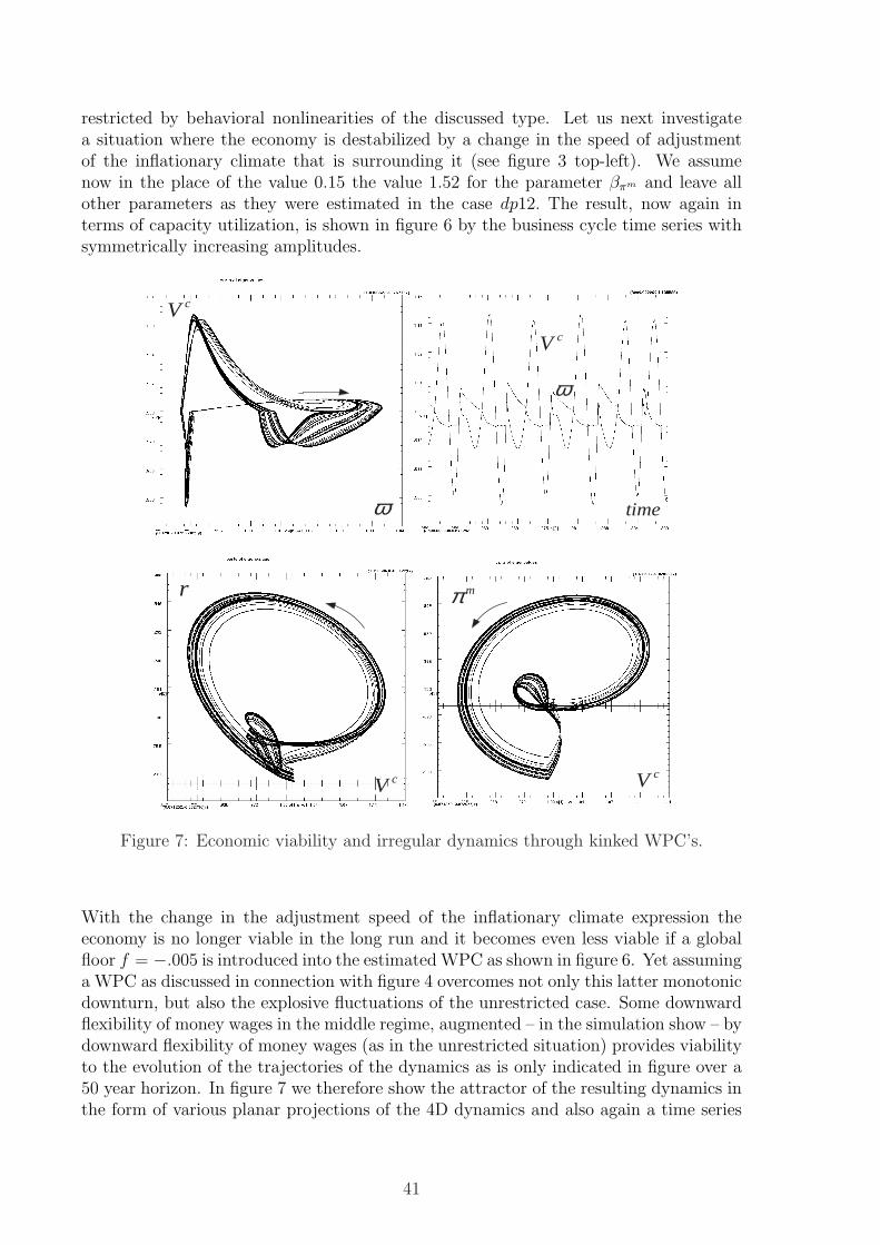
restricted by behavioral nonlinearities of the discussed type. Let us next investigatea situation where the economy is destabilized by a change in the speed of adjustmentof the inflationary climate that is surrounding it (see figure 3 top-left). We assumenow in the place of the value 0.15 the value 1.52 for the parameter βπm and leave allother parameters as they were estimated in the case dp12. The result, now again interms of capacity utilization, is shown in figure 6 by the business cycle time series withsymmetrically increasing amplitudes.

mπr

ω

cVcV

cVcV

time

ω

Figure 7: Economic viability and irregular dynamics through kinked WPC’s.

With the change in the adjustment speed of the inflationary climate expression theeconomy is no longer viable in the long run and it becomes even less viable if a globalfloor f = −.005 is introduced into the estimated WPC as shown in figure 6. Yet assuminga WPC as discussed in connection with figure 4 overcomes not only this latter monotonicdownturn, but also the explosive fluctuations of the unrestricted case. Some downwardflexibility of money wages in the middle regime, augmented – in the simulation show – bydownward flexibility of money wages (as in the unrestricted situation) provides viabilityto the evolution of the trajectories of the dynamics as is only indicated in figure over a50 year horizon. In figure 7 we therefore show the attractor of the resulting dynamics inthe form of various planar projections of the 4D dynamics and also again a time series

41

of the rate of capacity utilization over a time span of 250 years.18

We see in figure 7 projections of – from the mathematical point of view – complexattractor, which – from the economic point of view – is however only somewhat irregular.We can detect phases where economic activity rises without much change in real wages(and also the opposite) and phases where inflation without much change or even adecline in economic activity. The figure 7, bottom-right, shows the typical overshootingmechanism of here the interaction of capacity utilization with the inflationary climate,with stagflation occurring top-right in this phase plot. The interactions of interest ratesand economic activity is a cyclical one, with increased tensions and sudden turns atlow rates of interest. The interaction of the employment rate is partly clockwise, butalso partly counterclockwise. In sum, we therefore for the moment find that twicekinked Phillips curves as considered in Filardo (1998), here used for our WPC, cantame explosive behavior or even avoid economic breakdown, and will in fact give rise toeven complex dynamics if the adjustment of inflationary expectations introduces localinstability in an otherwise stable system with estimated parameter sizes. We finally notethat, on an average, the employment rate stays significantly below the normal level 1,the interest rate above its target level and the inflation climate below the target of thecentral bank, while capacity utilization fluctuates fairly symmetrically around its normallevel.

r r

r r

cV cV

cV cV

.41, .05cp Vγ γ= = .41, .2cp V

γ γ= =

.41, .4cp Vγ γ= =.2, .05cp V

γ γ= =

Figure 8: Monetary policy in regimes of irregular persistent business fluctuations .

In figure 8 finally we consider the issue of what monetary policy can achieve in such an

18Note that the phase length of the considered fluctuations must be a long one, since all parametersof the model are kept constant along these fluctuations, instead of varying systematically with as forexample discussed in the ’Notes on trade Cycle’ in Keynes General Theory.

42

environment. Top-left we show again the obtained complex dynamics for the estimatedparameters of the interest rate policy rule, there projected into the interest rate – infla-tionary climate phase plane. Increasing the reaction of the monetary authority to theutilization gap (from the estimated value 0.05 to 0.2) removes the complexity of the dy-namics and give rise to a limit cycle with considerably less amplitude and less deflationthan was the case before. We even get convergence and thus complete disappearanceof the business cycle for the further increased parameter value γV c = 0.4, though nottowards the interior steady state of the unrestricted model, but towards a depressedsituation with high interest rates and the stable deflation our kinked WPC does allowfor. By contrast, however, increasing the reaction of the central bank to the size of theobserved inflation gap will make the economy not more, but less stable, while indeed areduction in the already passive reaction strength (shown in figure 8, bottom-left) willagain remove the initial persistent cycle and lead to damped fluctuations, again notaround the interior steady state of the unrestricted dynamics, but to a steady state withcapacity utilization and nominal interest rate above and the other state variables belowthese steady state values.

We conclude from these few simulation examples, that our estimated Keynesian disequi-librium dynamics gives rise to a variety of interesting situations when certain kinks inmoney wage behavior and changes in the adjustment speed of our inflationary climateexpression is taken account of. These changes furthermore show that more further in-vestigation of such behavioral nonlinearities are needed, see Chen and Flaschel (2004)and Flaschel, Kauermann and Semmler (2004) for some attempts into this direction inthe case of the U.S. economy, and that the role of climate expressions must be furtheranalyzed in future extensions of the analysis here presented.

8 Conclusions and outlook

We have considered in this paper a significant extension and modification of the tradi-tional approach to AS-AD growth dynamics, primarily by way of an appropriate refor-mulation of the wage-price block of the model, that allows us to avoid the dynamicalinconsistencies of the traditional Neoclassical Synthesis. It also allowed us to overcomethe empirical weaknesses and theoretical indeterminacy problems of the New Neoclassi-cal Synthesis, the New Keynesian approach, that arise from the existence of only purelyforward looking behavior in baseline models of staggered price and wage setting. Con-ventional wisdom, based on the rational expectations approach, however is here used toavoid the latter indeterminacy problems by appriate extensions of the baseline modelthat enforce its total instability (the existence of only unstable roots), implying thatthe steady state represents the only bounded trajectory in the deterministic core of themodel (to which the economy then immediately returns when hit by a demand, supplyor policy shock).

By contrast, our alternative approach – which allows for sluggish wage as well as priceadjustment and also for certain economic climate variables, representing the medium-run evolution of inflation (and in Asada, Chen, Chiarella and Flaschel (2004) also ofexcess profitability) – completely bypasses the purely formal imposition of such bound-edness assumptions. Instead it allows to demonstrate in a detailed way, guided by theintuition behind important macroeconomic feedback channels, local asymptotic stability

43

under certain plausible assumptions (indeed very plausible from the perspective of Key-nesian feedback channels), cyclical loss of stability when these assumptions are violated(if speeds of adjustment become sufficiently high), and even explosive fluctuations in thecase of further increases of the crucial speeds of adjustment of the model. In the lattercase extrinsic behavioral nonlinearities have to be introduced in order to tame the explo-sive dynamics, for example as in Chiarella and Flaschel (2000, Ch.6,7) where a kinkedPhillips curve (downward wage rigidity) is employed to achieve global boundedness.

The stability features of this – in our view properly reformulated – Keynesian dynamicsare based on specific interactions of traditional Keynes- and Mundell-effects or real rateof interest effects with so-called Rose or real-wage effects, see Chiarella and Flaschel(2000) for their introduction, which in the present framework – for the estimated model– simply means that increasing wage flexibility is stabilizing and increasing price flex-ibility destabilizing, based on the estimated fact that aggregate demand here dependsnegatively on the real wage and due to the extended types of Phillips curves we haveemployed in our new approach to traditional Keynesian growth dynamics. The interac-tion of these three effects is what explains the obtained stability results under the in thiscase not very important assumption of myopic perfect foresight, on wage as well as priceinflation, and thus gives rise to a traditional type of Keynesian business cycle theory, notat all plagued by the anomalies of the textbook AS-AD dynamics, see Chiarella, Flascheland Franke (2004) for a detailed treatment and critique of this textbook approach.

Our model therefore provides an array of stability results, which however are narroweddown to damped oscilations when the model is estimated with data for the U.S. economyafter World War II. Yet, also in this strongly conbvergent case, there can arise stabilityproblems if the estimated linear WPC is modified to allow for some downward moneywage rigidities. In such a case, prices may fall faster than wages in a depression, leadingto real wage increases and thus to further reductions in economic activity, setting inmotion a downward deflations spiral with further and further increasing real wages untilin fact economic breakdown occurs. We have shown in this regard how the reestablish-ment of downward wage flexibility in situations that have become very severe may avoidthis economic breakdown, leading then to persistent business fluctuations of more or lessirregular type and thus back to a further array of interesting stability scenarios. Mone-tary policy can try to avoid such situations and preserve damped oscillatory behavior,primarily through the adoption of a target rate of inflation that is chosen sufficientlylarge, and in case of the establishment of persistent fluctuations of the above type, re-duce such fluctuations by an activation of its reaction to output gaps or a reduction ofits reaction to inflation gaps, as was shown by way of numerical examples. It is thereforenot obvious into which direction monetary policy should be changed in order to makethe economy less and not indeed more volatile.

The model of this paper will be numerically explored in a companion paper, Asada,Chiarella, Flaschel and Hung (2004), in order to analyze in greater depth, with andwithout the empirical background here generated, the interaction of the various feed-back channels present in the considered dynamics. At that point we will make use of LMcurves as well as Taylor interest rate policy rules, kinked Phillips curves and Blanchardand Katz error correction mechanisms in order to investigate in detail the various waysby which locally unstable dynamics can be made bounded and thus viable. The ques-tion then is which assumption on private behavior and fiscal and monetary policy – onceviability is achieved – can reduce the volatility of the resulting persistent fluctuations.

44

Our work on related models suggests that interest rate policy rule may not be sufficientto tame the explosive dynamics in all conceivable cases, or even make it convergent. Butwhen viability is achieved – for example by downward wage rigidity – we can then inves-tigate parameter corridors where monetary policy can indeed reduce the endogenouslygenerated fluctuations of this approach to Keynesian business fluctuations.

Taking all this together, our general conclusion here is that this framework not onlyovercomes the anomalies of the Neoclassical Synthesis, Stage I, but also provides acoherent alternative to its second stage, the New Keynesian theory of the business cycle,as for example sketched in Gali (2000). This alternative is based on disequilibrium inthe market for goods and labor, on sluggish adjustment of prices as well as wages and onmyopic perfect foresight interacting with certain economic climate expression with a richarray of dynamic outcomes that provide great potential for further generalizations. Someof these generalizations have already been considered in Chiarella, Flaschel, Groh andSemmler (2000) and Chiarella, Flaschel and Franke (2004). Our overall approach, whichmay be called a disequilibrium approach to business cycle modelling of mature Keynesiantype, thus provides a theoretical framework within which to consider the contributionsof authors such as Zarnowitz (1999) who also stresses the dynamic interaction of manytraditional macroeconomic building blocks.

References (to be adjusted)

Asada, T., Chiarella, C., Flaschel, P. and R. Franke (2003): Open EconomyMacrodynamics. An Integrated Disequilibrium Approach. Heidelberg: SpringerVerlag.

Asada, T., Chen, P., Chiarella, C. and P. Flaschel (2004): Keynesian dynam-ics and the wage-price spiral. A baseline disequilibrium approach. UTS Sydney:School of Finance and Economics.

Asada, T., Chiarella, C., Flaschel, P. and H. Hung (2004): Keynesian dy-namics and the wage-price spiral. Numerical Analysis of a Baseline DisequilibriumModel. UTS Sydney: School of Finance and Economics.

Barro, X. (1994): The aggregate supply / aggregate demand model. Review of Eco-nomics and Statistics, 575, 1 – 6.

Baxter, M and King, R (1999): Measuring business cycles: Approximate band-passfilters for economic time series. Eastern Economic Journal, 81:4, 575-5.

Blanchard, O.J. and L. Katz (2000): Wage dynamics: Reconciling theory andevidence. American Economic Review. Papers and Proceedings, 69 – 74.

Chen Pu (2003): Weak Exogeneity in Simultaneous Equations System. University ofBielefeld: Discussion Paper No. 502.

Chen, P. and Flaschel, P. (2004): Testing the dynamics of wages and prices for theUS economy. Bielefeld: Center for Empirical Macroeconomics. Working paper.

Chiarella, C. and P. Flaschel (2000): The Dynamics of Keynesian MonetaryGrowth: Macro Foundations. Cambridge, UK: Cambridge University Press.

45

Chiarella, C., P. Flaschel, G. Groh and W. Semmler (2000): Disequilibrium,Growth and Labor Market Dynamics. Heidelberg: Springer Verlag.

Chiarella, C., Flaschel, P. and R. Franke (2004): .A Modern Approach to Key-nesian Business Cycle Theory. Qualitative Analysis and Quantitative Assessment.Cambridge, UK: Cambridge University Press, to appear.

Flaschel, P. and H.-M.Krolzig (2004): Wage and price Phillips curves. An em-pirical analysis of destabilizing wage-price spirals. Oxford: Oxford University.Discussion paper.

Flaschel, P., Kauermann, G. and W. Semmler (2004): Testing wage and pricePhillips curves for the United States. Bielefeld University: Center for EmpiricalMacroeconomics, Discussion Paper.

Gali, J. (2000): The return of the Phillips curve and other recent developments inbusiness cycle theory. Spanish Economic Review, 2, 1 – 10.

Gali, J., Gertler, M. and J.D. Lopez-Salido (2003): Robustness of the Es-timates of the Hybrid New Keynesian Phillips Curve. Paper presented at theCEPR Conference: The Phillips curve revisited. Berlin: June 2003

Groth, C. (1992): Some unfamiliar dynamics of a familiar macromodel. Journal ofEconomics, 58, 293 – 305.

Eller, J.W. and R.J. Gordon (2003): Nesting the New Keynesian Phillips Curvewithin the Mainstream Model of U.S. Inflation Dynamics. Paper presented at theCEPR Conference: The Phillips curve revisited. Berlin: June 2003

Mankiw, G. (2001): The inexorable and mysterious tradeoff between inflation andunemployment. Economic Journal, 111, 45 – 61.

Rose, H. (1967): On the non-linear theory of the employment cycle. Review of Eco-nomic Studies, 34, 153 – 173.

Rudebusch, G.D. and L.E.O. Svensson (1999): Policy rules for inflation targeting.In: J.B.Talor (ed.): Monetary Policy Rules. Chicago: Chicago University Press.

Sargent, T. (1987): Macroeconomic Theory. New York: Academic Press.

Tobin, J. (1975): Keynesian models of recession and depression. American EconomicReview, 65, 195 – 202.

Woodford, M. (2003): Interest and Prices. Princeton: Princeton University Press.

Zarnowitz, V. (1999): Theory and History Behind Business Cycles: Are the 1990sthe onset of a Golden Age? NBER Working paper 7010,http://www.nber.org/papers/w7010.

46

9 Appendix: Estimation Results

System-Estimate: \pi24

Linear Systems - Estimation by System Instrumental Variables

Iterations Taken 2Quarterly Data From 1965:01 To 2002:04Usable Observations 141Total Observations 152 Skipped/Missing 11

Dependent Variable DWCentered R**2 0.575957 R Bar **2 0.483774Uncentered R**2 0.924109 T x R**2 130.299Mean of Dependent Variable 0.0144658956Std Error of Dependent Variable 0.0067780095Standard Error of Estimate 0.0048699237Sum of Squared Residuals 0.0027273581Durbin-Watson Statistic 1.729474

Variable Coeff Std Error T-Stat Signif*******************************************************************************1. DP 0.742146755 0.1742780244.25841 0.00002059 2. \PI24 0.3709280800.258063828 1.43735 0.15061853 3. VL{1}0.130083208 0.050842531 2.55855 0.01051094 4. UCBP{1}-0.083710765 0.035544840 -2.35508 0.01851897 5. Constant-0.119681460 0.048707479 -2.45715 0.01400452

Dependent Variable DPCentered R**2 0.741782 R Bar **2 0.682891Uncentered R**2 0.937025 T x R**2 132.120Mean of Dependent Variable 0.0107048312Std Error of Dependent Variable 0.0061013171Standard Error of Estimate 0.0034358019Sum of Squared Residuals 0.0013457398Durbin-Watson Statistic 1.756548

Variable Coeff Std Error T-Stat Signif*******************************************************************************6. DW 0.542721944 0.0587209859.24238 0.00000000 7. \PI24 0.5455242160.075159486 7.25822 0.00000000 8. VC{1}

47

0.029690971 0.006570948 4.51852 0.00000623 9. UCBP{1}0.091781957 0.022814773 4.02292 0.00005748 10. D740.006062371 0.001735776 3.49260 0.00047834 11. Constant-0.027228957 0.005453445 -4.99298 0.00000059

Dependent Variable DLVLCentered R**2 0.635807 R Bar **2 0.567907Uncentered R**2 0.635925 T x R**2 89.665Mean of Dependent Variable 0.0000643400Std Error of Dependent Variable 0.0035883459Standard Error of Estimate 0.0023587552Sum of Squared Residuals 0.0006565197Durbin-Watson Statistic 1.431341

Variable Coeff Std Error T-Stat Signif*******************************************************************************12. DLVC 0.2091319356 0.0144254835 14.49740 0.0000000013. Constant 0.0001859823 0.0001763756 1.05447 0.29166905

Dependent Variable DLVCCentered R**2 0.403475 R Bar **2 0.280056Uncentered R**2 0.404114 T x R**2 56.980Mean of Dependent Variable -0.000581654Std Error of Dependent Variable 0.017816411Standard Error of Estimate 0.015117141Sum of Squared Residuals 0.0265092413Durbin-Watson Statistic 1.334401

Variable Coeff Std Error T-Stat Signif*******************************************************************************14. VC{1} -0.093805470 0.026035675 -3.60296 0.0003146215. RRATE{1} -0.173880204 0.044069044 -3.94563 0.0000795916. UCBP -0.744305360 0.127462642 -5.83940 0.0000000117. Constant 0.086219485 0.021848091 3.94632 0.00007936

Dependent Variable RATECentered R**2 0.889129 R Bar **2 0.866190Uncentered R**2 0.982857 T x R**2 138.583Mean of Dependent Variable 0.0712450355Std Error of Dependent Variable 0.0305780815Standard Error of Estimate 0.0111854768Sum of Squared Residuals 0.0145133273Durbin-Watson Statistic 1.717594

Variable Coeff Std Error T-Stat Signif*******************************************************************************18. DP 0.426569670 0.169847604 2.51148 0.0120224519. VC{1} 0.045860894 0.020205006 2.26978 0.0232210120. RATE{1} 0.900706175 0.035391750 25.44961 0.00000000

48

21. Constant -0.034790497 0.016931833 -2.05474 0.03990422

Covariance\Correlation Matrix of ResidualsDW DP DLVL DLVC RATE

DW 0.00001934297 -0.8808113407 -0.0769496687 -0.0757498777 -0.1304136539DP -0.00001196783 0.00000954425 -0.0508887611 0.1207371612 0.1294293357DLVL -0.00000073027 -0.00000033924 0.00000465617 -0.3872194428 -0.0668326528DLVC -0.00000456807 0.00000511447 -0.00001145673 0.00018800880 0.5109124741RATE -0.00000581914 0.00000405674 -0.00000146311 0.00007107380 0.00010293140






Dependent Variable DPCentered R**2 0.806935 R Bar **2 0.762903Uncentered R**2 0.952915 T x R**2 134.361Mean of Dependent Variable 0.0107048312Std Error of Dependent Variable 0.0061013171Standard Error of Estimate 0.0029708892Sum of Squared Residuals 0.0010061848Durbin-Watson Statistic 1.702034

Variable Coeff Std Error T-Stat Signif*******************************************************************************

49

6. DW 0.336057879 0.0731191224.59603 0.00000431 7. \PI12 0.6817049650.081901222 8.32350 0.00000000 8. VC{1}0.034327378 0.006749461 5.08594 0.00000037 9. UCBP{1}0.064237346 0.021147879 3.03753 0.00238525 10. D740.007869569 0.001745077 4.50958 0.00000650 11. Constant-0.029547353 0.005457849 -5.41374 0.00000006





Dependent Variable RATECentered R**2 0.889087 R Bar **2 0.866140Uncentered R**2 0.982850 T x R**2 138.582Mean of Dependent Variable 0.0712450355Std Error of Dependent Variable 0.0305780815Standard Error of Estimate 0.0111875877Sum of Squared Residuals 0.0145188059Durbin-Watson Statistic 1.720381

Variable Coeff Std Error T-Stat Signif*******************************************************************************

50

18. DP 0.412678154 0.170978227 2.41363 0.0157945019. VC{1} 0.049245320 0.020250914 2.43176 0.0150257520. RATE{1} 0.902140081 0.035309913 25.54920 0.0000000021. Constant -0.037507088 0.016965122 -2.21084 0.02704726


DW 0.00001801540 -0.6927029730 -0.0446864666 -0.0453206036 -0.1118783388DP -0.00000785413 0.00000713606 -0.0375454185 0.1912816213 0.1742782419DLVL -0.00000041356 -0.00000021869 0.00000475414 -0.4108331850 -0.0870687804DLVC -0.00000264207 0.00000701826 -0.00001230350 0.00018864879 0.5126235990RATE -0.00000481863 0.00000472420 -0.00000192644 0.00007144659 0.00010297025






Dependent Variable DPCentered R**2 0.832232 R Bar **2 0.793969Uncentered R**2 0.959084 T x R**2 135.231

51

Mean of Dependent Variable 0.0107048312Std Error of Dependent Variable 0.0061013171Standard Error of Estimate 0.0027694288Sum of Squared Residuals 0.0008743499Durbin-Watson Statistic 1.747540

Variable Coeff Std Error T-Stat Signif*******************************************************************************6. DW 0.177078861 0.0838578392.11166 0.03471601 7. \PI6 0.8248037840.089209229 9.24572 0.00000000 8. VC{1}0.028436521 0.006116308 4.64930 0.00000333 9. UCBP{1}0.030970638 0.021627119 1.43203 0.15213584 10. D740.007316561 0.001775362 4.12116 0.00003770 11. Constant-0.023573580 0.004863736 -4.84680 0.00000125





Dependent Variable RATECentered R**2 0.889093 R Bar **2 0.866147Uncentered R**2 0.982851 T x R**2 138.582

52

Mean of Dependent Variable 0.0712450355Std Error of Dependent Variable 0.0305780815Standard Error of Estimate 0.0111872870Sum of Squared Residuals 0.0145180254Durbin-Watson Statistic 1.719811

Variable Coeff Std Error T-Stat Signif*******************************************************************************18. DP 0.436354636 0.172619081 2.52785 0.0114764319. VC{1} 0.049608273 0.020259936 2.44859 0.0143416720. RATE{1} 0.900497767 0.035458792 25.39561 0.0000000021. Constant -0.037940151 0.016971735 -2.23549 0.02538517


DW 0.00001780791 -0.3668130112 -0.0735320861 0.0071825216 -0.1002736397DP -0.00000385464 0.00000620106 -0.0987427905 0.2880260143 0.1636919701DLVL -0.00000067949 -0.00000053844 0.00000479509 -0.4197416135 -0.0904398589DLVC 0.00000041656 0.00000985732 -0.00001263208 0.00018888110 0.5124650125RATE -0.00000429376 0.00000413623 -0.00000200957 0.00007146653 0.00010296472

53

Keynesian Dynamics and the Wage-Price Spiral. Estimating ...

Documents

Transcript of Keynesian Dynamics and the Wage-Price Spiral. Estimating ...