Estimating The Demand for School Attributes in...

Estimating The Demand for School Attributes in

Pakistan

Pedro CarneiroUniversity College London, Institute for Fiscal Studies and

Centre for Microdata Methods and Practice

Jishnu DasWorld Bank

Hugo Reis∗

University College London

February 2010

[Preliminary Version]

Abstract

This paper studies the determinants of parental choices of school at-tributes in Pakistan, a country where a long fraction of schools are private.We estimate a standard model of demand for differentiated products usinga rich dataset with school attributes, household and child characteristics,and school choices. We find that a one-standard deviation increase in thequality of basic facilities is valued at about 210 rupees, which correspondsto an increase of the average school fee by around 45 per cent. In termsof distance, a one standard deviation decrease (on average an 800 meterdecrease) is valued at about 180 rupees. There is some evidence that thedeterminants of school choice change with household/student characteris-tics, like gender and parents education, in particular regarding price anddistance.

Keywords: Education, School Choice, Pakistan, Demand, Discretechoice model

JEL Classification:I20,I21

1 Introduction

Although the study of the effect of school competition on school quality is ex-tensive, this topic is still one of the most important in the field of educationaleconomics and at an educational policy level, in particular in the US and UK.

∗E-mail: [email protected]; [email protected]; [email protected].

1

In the last decade, many empirical studies emerged in the U.S. (a good exampleis Hoxby (2003) and more recently Hastings, Kane and Staiger (2009)) and thequality of educational institutions became a worldwide concern. School choice isone of the most debated policies aimed at increasing welfare1. Those in favouradvocate that school choice may create incentives for schools to increase produc-tivity, offering a product closer to students demand, and expand the choice setfor poor students. In contrast, opponents argue that school choice may increasesegregation, may decrease school quality to poor students by moving good peersto other schools, and may produce competition in irrelevant attributes if parentsare careless about educational outcomes.

This paper studies the determinants of parents choices among different schoolswhen they are allowed to do so. Do they consider price?, quality? distance?.This line of research is relevant from a policy perspective as it allows to havea clear understanding of how students are allocated to schools in equilibrium.An extended literature have analysed this topic: i) simple logit models for thechoice between different type of schools (for example, Alderman, Orazem andPatterno (2001) for Pakistan, Checchi and Japelli (2004) for Italy), ii) struc-tural choice models using information on a particular area (Bayer and McMillan(2006)and iii) mixed logit models with information about the first and secondchoices in a particular area (Hastings, Kane and Staiger (2009) and Hastingsand Weinstein (2007)) and iv) logit model for the choice of an individual schoolbetween public and voucher schools (Gallego and Hernando (2009) for Chile)2.

We extend the literature to a developing country using detailed informationon the school choices in Punjab province, the largest state in Pakistan, in acontext in which parents can choose among all schools (public and private)3.During the 1970’s Pakistan actively discouraged private schooling, to the pointof nationalizing many private schools. While this policy was reversed in thefollowing decade, the trend towards private schools has accelerated in recentyears. For example, the number of primary private schools increased more than10 times in the last 25 years (47000 in 2005 compared with 3800 in 1983).Therefore, some characteristics of the Pakistani educational system make thestudy of school choice interesting. In Pakistan, not only parents are allowed to

1A good example is the Chilean education voucher system2Their approach is similar to the approach presented in this paper. However, it does not

take into account random coefficients and the choice set includes only public and voucherschools (private schools accounts for more than 10 per cent of total enrollment)

3Gallego and Hernando (2009) allows more choice than the public schools considering alsothe choice of voucher schools. However, they do not take into account the non-free privateschools, which account for more than 10 per cent of total enrollment.

2

choose freely the school without any restriction as the ”creation” of a privateschool is relatively simple. These schools are usually familiar enterprises purelydriven by their own revenues and facing little government regulation (Andrabiet al 2007). They offer Western education type in a coeducational environment,in particular at the primary level. Another important characteristic of theseschools is that the typical rural private school is very affordable what explainsthe recent trend in the number of private schools. In 2000, a national level censusof private school shows that the median fee charged by a private school is about60 rupees per month (around a day’s unskilled wage). Public schools charge nofees. These characteristics play all in favour of expansion of school choice inPakistan, which is shown in our sample. In Punjab, the largest province in thecountry, the educational marketplace seems reasonably competitive. A tipicalvillage is serviced, on average, by 7 different schools (public and private).

We model school choice of a household as a discrete choice model of a singleschool. The utility function specification is based on the random utility modeldeveloped by McFadden (1974) and the specification of Berry, Levinsohn, andPakes (BLP) (2004), which includes choice-specific unobservables characteris-tics combining macro and micro data. In our model, the allocation of studentsto schools is allowed to vary with household’s own characteristics.A central empirical issue is whether the sources of consumer heterogeneity, typ-ically available in micro data sets (income, household demographics, locationof residence), are rich enough to account for the heterogeneity in tastes for dif-ferent characteristics. Our model allows tastes for characteristics to vary as afunction of both observed and unobserved consumer attributes.

The results suggest that the most relevant determinants of parents’ choicesamong different schools are price, distance and basic infrastructure. We findthat a one-standard deviation increase in the quality of basic facilities is valuedat about 210 rupees, which corresponds to an increase of the average schoolfee by around 45 per cent. In terms of distance, a one standard deviationdecrease (on average an 800 meter decrease) is valued at about 180 rupees.Other quality characteristics, like test scores, seem not to be as important forthe parents decision as it is in other countries like in the US 4. There is someevidence that the determinants of school choice change with household andstudent characteristics, like gender and parents education, in particular in termsof price and distance.

4In Chile there is also some evidence of the importance of test scores on parents’ schooldecision

3

The remaining of this paper is organised as follows. Section 2 presents theData. Section 3 describes the econometric model used to study the determinantsof parents choices among different schools. Section 4 presents the results. FinallySection 5 concludes.

2 Data

This paper uses the Learning and Education Achievement in Punjab School(LEAPS) project data set5. The LEAPS data is collected from 112 villages inthe Punjab province, the largest state in Pakistan, located in the three districtsof Attock (North), Faisalabad (Center), and Rahim Yar Khan (South). Villageswere randomly chosen from a list of villages with at least one private schoolaccording to the 2000 census of private schools. This allows us to look at dif-ferences between private and public schools in the same village. The baselinesurvey in 2004 covered 823 schools (government and private) and around 1800households (with almost 6000 children).

We use school characteristics, students background, their educational outcomesand parent preferences data. Table 1 presents the variables used and a briefdescription of each variable.We use Math average test scores to measure academic outcomes. To measureother characteristics of school, we use school fees payed by the students andinfrastructure facilities (basic and extra)6 We consider teacher absenteeism andteacher test scores as measures of teacher quality.In addition, we include information on the distance from the place where thestudent lives and all schools in the village. At the student level we use parentseducation, age and gender. As a proxy measure of household income per capitawe use expenditure per capita .

Table 2 presents summary statistics for the attributes we use at the schoollevel. In our sample, almost 40 per cent of the schools are private and the

5The project details are available at www.leapsproject.org6School basic facilities: number of permanent classrooms, semi-permanent classrooms,

staffrooms, stores, toilets(combined), toilets(boys), toilets(girls), and blackboards per student(including nursery students).School extra facilities: whether school has library, computers, sports equipment, meeting hall,surrounding wall or fence, fans, and electricity.

4

average private school fee paid by the parents is around 1120 rupees per year.Overall, there is a considerable variance of school characteristics.Table 3 illustrates descriptive statistics at the household and student level.Around 75 per cent of the children attend school and around 16 per cent neverattended school. The average age of the children is 10 years old. In terms ofdistance to school, it is interesting to notice that boys travel, on average, morethan girls. The total monthly household expenditure per capita is around 950rupees, almost the same amount parents spent on average per year to keep achild in a private school.Table 4 describes data of the school attributes divided by parents educationand income. As expected, more educated parents have a higher percentage ofchildren in private schools and thus pay more (around two times on average)for school fees. In addition, more educated parents have children in schoolswith better infrastructures, lower teacher absenteeism and slightly higher av-erage test scores. In terms of income, the results are in general similar andas expected. Wealthier parents have more children in private schools (payinghigher fees) and children tend to travel less. Moreover, wealthier householdshave their children in schools with better infrastructures, higher average testscores (despite relatively small) and lower teacher absenteeism.

3 Model

Several methods have been used to estimate models of demand for differentiatedproducts in the presence of endogenous explanatory variables. In this paper, wedescribe the most often used procedure in the literature, developed by Berry,Levishon and Pakes (BLP) 2004, which includes choice-specific unobservablecharacteristics combining macro and micro data.

3.1 BLP approach

The indirect utility of household i get from its child (of gender g) attendingschool j in village t is given by

uijtg =K∑k=1

xjktgβik + γidijtg + λjtg + εijtg (1)

5

where

j = {0, ..., J} index schools competing in the market tg; j = 0 is the ”out-side” good such that ui0tg is the utility the individual derives if he does not goto any of the J schools.

i = {1, ..., N} index indviduals,

t = {1, ...T} index mauzas (villages),

g = {male, female},

k index the observed school characteristics and

r index the observed individual characterisitcs.

Let Xjk = {xj1,xj2,...,xK} be observed school characteristics,

λj unobserved school attributes valued equally by everyone,

dij− distance from the house of the household i to school j.

Zi = {zi1,zi2,...,ziR} observable individual characteristics,

vi unobservable characteristics of household i and

εijtg individual-specific preference for school j in market tg assumed to havean extreme value type I distribution.

The value of school’s characteristics is allowed to vary with household’s owncharacteristics according to:

βik = βk +R∑r=1

zirtgβork + βuk vitg (2)

and

γi = γ +R∑r=1

zirtgγr + γuvitg (3)

6

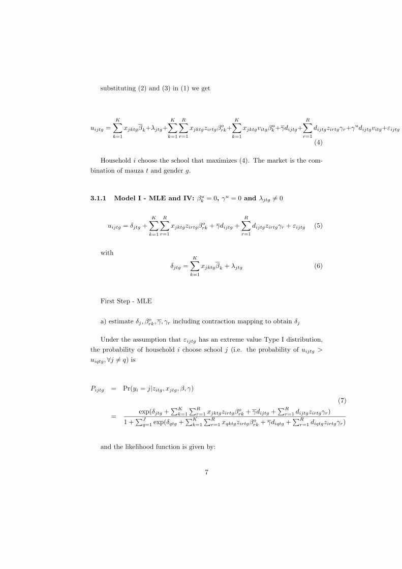
substituting (2) and (3) in (1) we get

uijtg =K∑k=1

xjktgβk+λjtg+K∑k=1

R∑r=1

xjktgzirtgβork+

K∑k=1

xjktgvitgβuk+γdijtg+

R∑r=1

dijtgzirtgγr+γudijtgvitg+εijtg

(4)

Household i choose the school that maximizes (4). The market is the com-bination of mauza t and gender g.

3.1.1 Model I - MLE and IV: βuk = 0, γu = 0 and λjtg 6= 0

uijtg = δjtg +K∑k=1

R∑r=1

xjktgzirtgβork + γdijtg +

R∑r=1

dijtgzirtgγr + εijtg (5)

with

δjtg =K∑k=1

xjktgβk + λjtg (6)

First Step - MLE

a) estimate δj , βork, γ, γr including contraction mapping to obtain δj

Under the assumption that εijtg has an extreme value Type I distribution,the probability of household i choose school j (i.e. the probability of uijtg >uiqtg,∀j 6= q) is

Pijtg = Pr(yi = j|zitg, xjtg, β, γ)

(7)

=exp(δjtg +

∑Kk=1

∑Rr=1 xjktgzirtgβ

ork + γdijtg +

∑Rr=1 dijtgzirtgγr)

1 +∑Jq=1 exp(δqtg +

∑Kk=1

∑Rr=1 xqktgzirtgβ

ork + γdiqtg +

∑Rr=1 diqtgzirtgγr)

and the likelihood function is given by:

7

L(β, γ) =J∏j=1

∏i∈Aj

Pijtg

and the log-likelihood by:

LL(β, γ) =∑Jj=1

∑i∈Aj

ln(Pijtg)

where, the set of households that choose school j is given by

Ajtg(xjtg, dijtg; δjtg, βork, γ, γr) = {(εi0tg, ..., εiJtg)|uijtg > uiltg,∀j 6= l}

Partially differentiating (7) with respect to δqtg we get

∂LL

∂δqtg=

J∑j=1j 6=q

∑i∈Aj

1Pijtg

∂Pijtg∂δqtg

+∑i∈Aq

1Piqtg

∂Piqtg∂δqtg

(8)

Given that

∂Piqtg∂δqtg

= Piqtg(1− Piqtg) (9)

∂Pijtg∂δqtg

= −PiqtgPijtg, j 6= q (10)

the FOC with respect to δqtg of the Maximum Likelihood (ML) problembecomes:

∂LL

∂δqtg=

∑i∈Aq

1−J∑j=1

∑i∈Aj

Piqtg

= Nq −N∑i=1

Piqtg = 0

8

Dividing by N we get:

shq −1N

N∑i=1

Piqtg = 0 (11)

where shq is the share of students that attend school q and N is the totalnumber of students.

This condition implies that the estimated δjtg has to guarantee that theempirical share of student attending school j has to be equal to the averageprobability that a student attends this school.

In order to find estimates for the parameters of interest we need to iterateover

δt+1qtg = δtqtg −

[log(shq)− log(

1N

N∑i=1

Piqtg)

](12)

Each iteration over (12) requires a new calculation of the probabilities in (7)

Second Step - IV

b) estimate βk

The second step is the estimation of the school fixed effect (δjtg) on theobserved school characteristics as in equation (6).

School fees and test score variables may be correlated with the unobservedquality characteristics of the school, which lead OLS estimation to be biased. Atthis stage, a natural issue arises to define which variables to use as instruments.BLP proposed to use the observed non-price attributes of other schools. Theidea is that each firm will price its products taking into account the substitutionwith other firms products. We assume that the price charged by one schoolis correlated with the observable characteristics of other schools in the samemarket. Following BLP, and assuming that the unobservable attributes of schoolj (λj) are not dependent of its non-price and non-test score characteristics(Xj� {pricej , test scorej}) , the non-price and non-test scores attributes ofother schools in the same market (X−j� {price−j , test score−j}) are used asinstruments.

9

3.1.2 Model II - Maximum Simulation Likelihood (MSL) and IV:

βuk 6= 0, γu 6= 0 and λjtg 6= 0

uijtg = δjtg+K∑k=1

R∑r=1

xjktgzirtgβork+

K∑k=1

xjktgvitgβuk+γdijtg+

R∑r=1

dijtgzirtgγr+dijtgvitgγu+εijtg

(13)

with

δjtg =K∑k=1

xjktgβk + λjtg (14)

First Step - MSL

a) estimate δj , βork, βuk , γ, γr, γ

u including contraction mapping to obtain δj .

Let P̃iqtg be a simulated approximation to Piqtg. The simulated choice prob-ability is given by

P̃ijtg =

ND∑n=1

exp(δjtg +∑K

k=1∑R

r=1 xjktgzirtgβork + γdijtg +

∑Rr=1 dijtgzirtgγr +

∑Kk=1 xjktgvitgnβ

uk + dijtgvitgnγ

u)

1 +∑J

q=1 exp(δqtg +∑K

k=1∑R

r=1 xqktgzirtgβork + γdiqtg +

∑Rr=1 diqtgzirtgγr +

∑Kk=1 xqktgvitgnβu

k + diqtgγu)

for random draws vitgn, n = 1, ..., ND.

The Simulated log-likelihood function is given by

SLL(β, γ) =∑Jj=1

∑i∈Aj

ln(P̃ijtg)

This procedure is the same as ML except that simulated probabilities areused instead of the exact probabilities.

Second Step - IV

b) estimate βk

The second step is the estimation of the school fixed effects (δjtg) on theobserved school characteristics as before and in equation (14).

10

4 Results

BLP approach

Model I - no random coefficients (βuk = 0, γu = 0)

Table 5 panel A presents the estimation results of βk, the direct effects. Theanalysis will focus on the OLS and IV estimates in column (3) and (4), whichcontrols for village characteristics. As expected, estimates suggest that schoolsthat charge higher fees and are located at a higher distance tend to be lesspreferred by parents. In turn, parents tend to prefer schools with more/betterbasic infrastructures (e.g. toilets). In general, with the expected sign but notstatistically significant we have characteristics like average students test scores,extra infrastructures, teacher absenteeism and teacher test scores. In terms ofeconomic significance of these estimates, we get that a one-standard deviationincrease in basic facilities is valued at about 210 rupees, which corresponds toan increase of the average school fee by around 45 per cent. In terms of distance,a one standard deviation decrease (on average an 800 meter decrease) is valuedat about 180 rupees. In general, the results are similar to the ones presented incolumn (1) and (2) where there is no controls for village characteristics.

Table 6 panel A presents the interaction results to study the degree of het-erogeneity in terms of preferences for school attributes depending on observablestudent characteristics. More educated parents are willing to pay more schoolfees and tend to put more weight on extra facilities and Teacher Test scoresand less weight on basic facilities. Wealthier families tend to put more weighton extra facilities, less on basic facilities and are willing to pay more for schoolfees. In addition, although parents are willing to pay less for a girl student,characteristics like extra facilities and average test scores seem to be more im-portant. Also, less distant schools seems to be more relevant if the chidren is agirl. Moreover, if the children is younger, parents are willing to pay more andfeatures like basic infrastructures and test scores seem to be more important.In terms of teacher abseenteeism there seems to be no heterogeneity.

Model II - random coefficients βuk 6= 0, γu 6= 0

Table 5 panel B presents the direct effects results of the model when weinclude choice-specific unobservables characteristics. These results are in line

11

with the ones presented by model I. Parents tend to prefer schools i) that chargelower fees, ii) that are located at a smaller distance and iii) with more/betterbasic infrastuctures.

Table 6 panel B describes the interaction results to study the degree of het-erogeneity in terms of preferences for school attributes depending on observablestudent characteristics. In this model, the degree of heterogeneity is smaller.The remaining effects are the ones regarding price and distance. More educatedand richer parents are willing to pay more for children education and less distantschools seems to be more relevant if the chidren is a girl.

Table 7 describes the interaction results to study the degree of heterogeneityin terms of preferences for school attributes depending on unobservable studentcharacteristics. These results indicate that we do not need additional unob-served interactions to explain the data.

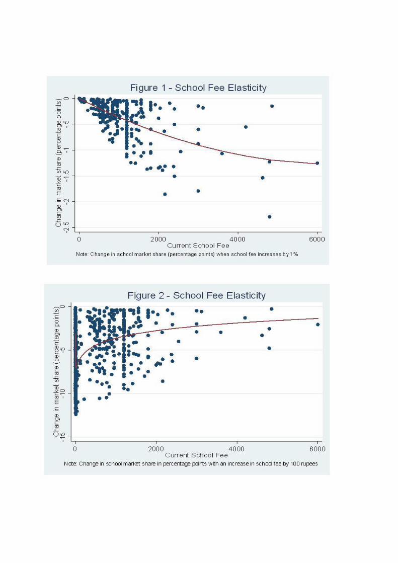
School Fee Elasticity

Figure 1 and 2 present two measures of school fee elasticity. Figure 1 con-siders the impact on private schools market shares when the price increases by1 per cent. In this case, we have a negative relation between current prices andchanges in the market share. Therefore, more expensive private schools presenta higher elasticity (highest reduction in their market share due to a 1 per centincrease in prices). The most affected schools would see their market share re-duced by 2.3 p.p. (on average the market share per private school is reducedby around 0.4 p.p.). In Figure 2 we look at the effect of an increase in pricesby 100 rupees on the school market share in percentage points (p.p), includingpublic schools in the analyses. In this figure we have a positive relation betweencurrent prices and changes in the market share. In fact, public schools and pri-vate schools charging lower prices have a bigger impact on their share comparedwith more expensive private schools. Market share decreases on average 5 p.p,reaching a maximum of almost 12.5 p.p in some public schools.

5 Conclusion

School choice is one of the most debated topic and one of the most important inthe educational economics field. In fact, the quality of educational institutions

12

become a worldwide concern, including the developing countries. Our study ofthe demand side of the Pakistani education system can help us understand theeffects of choice (in particular the widespread supply of affordable private insti-tutions) on educational outcomes and household/student welfare. This paperpresents estimates of the demand side of school choice allowing the allocationof students to vary with household own characteristics (observable and unob-servable). These estimates are essential to understand the effects of increasedchoice and potential responses from the supply side. In addition, they allow thestudy of different implications in terms of education policy. Our results suggestthat the most relevant determinants of parents’ choices among different schoolsare price, distance and basic infrastructure. There is some evidence that the de-terminants of school choice change with household/student characteristics, likegender and parents education, in particular regarding price and distance. Theseestimates will allow us to study the effects of school choice on consumer(student)welfare through policy simulations. Using compensation variation to measurechanges in student welfare related to changes in the design of the school choicesystem. This particular effect is the aim of future and ongoing research.

References

[1] Ackeberg D., Benkard C., Berry, S. and Pakes A. (2007) “Econometric Toolsfor Analyzing Market Outcomes” Handbook of Econometrics, vol.6A, Ch.63,4172-4276

[2] Andrabi T., Das J., Khwaja A., Vishwanath T. and Zajonc, T. (2007) “TheLearning and Educational Achievement in Punjab Schools (LEAPS) Report”, Oxford University Press, Pakistan (forthcoming)

[3] Bayer P., Ferreira, F. and McMillan R. (2007) “A Unified Framework forMeasuring Preferences for Schools and Neighborhoods” Journal of PoliticalEconomy, vol. 115, 4, 588-638

[4] Berry, S., Levinsohn J. and Pakes A. (1995). “Automobile prices in marketequilibrium”, Econometrica, 63, 841-889 .

[5] Berry, S., Levinshon J. and Pakes A. (2004). “Differentiated Products De-mand Systems from a Combination of Micro and Macro Data: The New CarMarket”, Journal of Political Economy, vol. 112 , 3, 68-105

13

[6] Berry, S. and Haile, P. (2009). “Nonparametric Identification of MultinomialChoice Demand Models with Heterogeneous Consumers”, NBER Workingpaper No. 15276

[7] Gallego F., and Hernando, A. (2009). “School Choice in Chile: Lookingat the demand side”, Documento de Trabajo 356, Pontificia UniversidadCatolica Chile

[8] Hastings J., Kane, T. and Staiger D. (2009). “Heterogeneous Preferences andthe Efficacy of Public School Choice”, Revise and Resubmit, Econometrica.Combines and replaces National Bureau of Economic Research Paper Work-ing Papers No. 12145 and No. 11805. June (2008).

[9] Hastings J. and Weinstein (2007). “No Child Left behind: Estimating theimpact on choices and student outcomes”, NBER Working paper No. 13009

[10] Petrin A. (2002). “Quantifying the benefits of new products: The case ofthe minivan”, Journal of Political Economy, vol. 110, 4, 705-729.

[11] Train K. (2009). “Discrete Choice Methods with Simulation”, CambridgeUniversity Press, Second edition

14

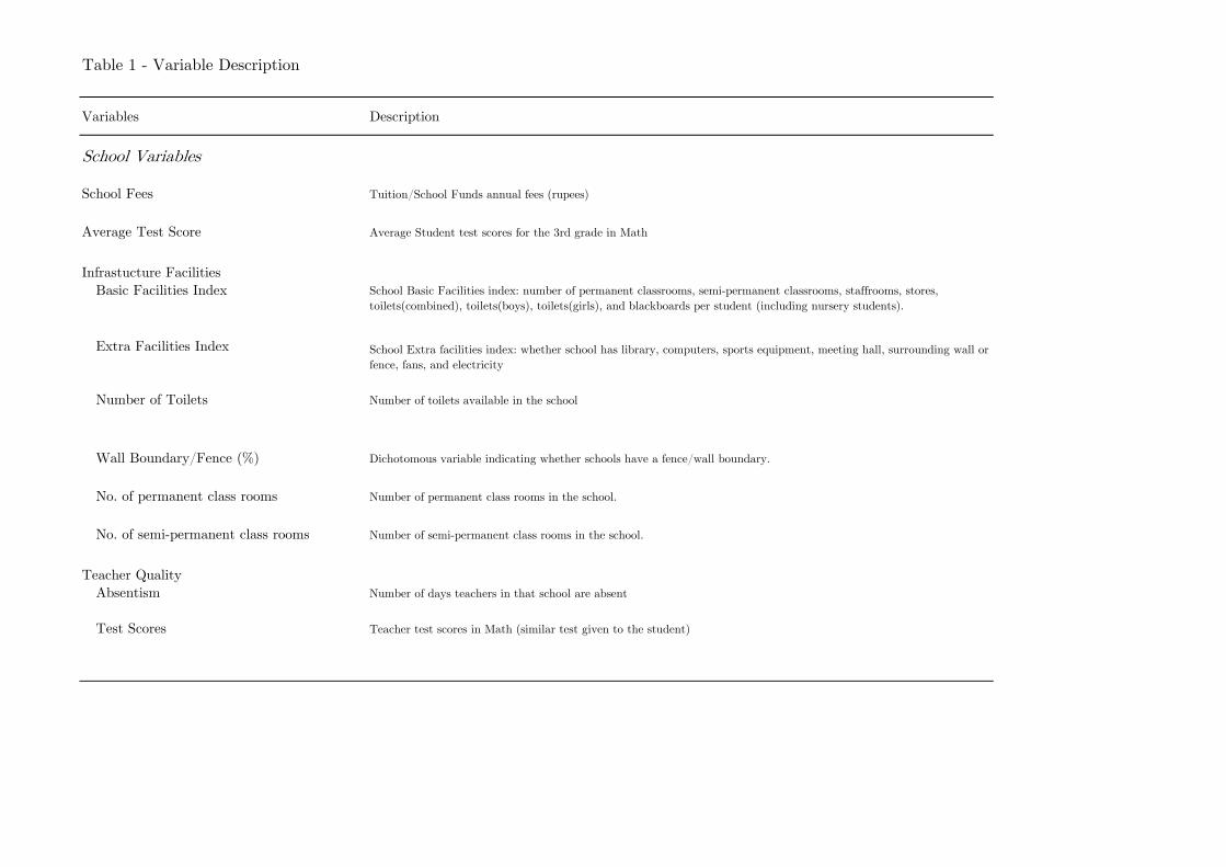
Table 1 - Variable Description

Variables Description

School Variables

School Fees Tuition/School Funds annual fees (rupees)

Average Test Score Average Student test scores for the 3rd grade in Math

Infrastucture Facilities

Basic Facilities Index

Extra Facilities Index

Number of Toilets Number of toilets available in the school

Wall Boundary/Fence (%) Dichotomous variable indicating whether schools have a fence/wall boundary.

No. of permanent class rooms Number of permanent class rooms in the school.

No. of semi-permanent class rooms Number of semi-permanent class rooms in the school.

Teacher Quality

Absentism Number of days teachers in that school are absent

Test Scores Teacher test scores in Math (similar test given to the student)

School Basic Facilities index: number of permanent classrooms, semi-permanent classrooms, staffrooms, stores,

toilets(combined), toilets(boys), toilets(girls), and blackboards per student (including nursery students).

School Extra facilities index: whether school has library, computers, sports equipment, meeting hall, surrounding wall or

fence, fans, and electricity

Table 1 (cont.) - Variable Description

Variables Description

Individual/household characteristics

Girl Dichotomous variable indicating whether a student is a girl.

Age of the child Reports the child's age in years.

School Attendance Dichotomous variable indicating whether a children is attending school.

Distance to school (Kms) Reports the distance in Kms from the house to any school available in the village.

Parents Education

Father Education Reports the students's father years of education.

Mother Education Reports the students's mother years of education.

Highest Parent Education Reports the highest level of students's parents years of education.

Proxy of Income

Total Expenditure Total monthly expenditure

Household size Number of people living in the household

Expenditure per "capita" Total monthly expenditure divided by household size

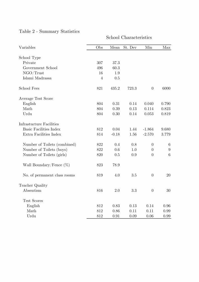
Table 2 - Summary Statistics

Variables Obs Mean St. Dev Min Max

School Type

Private 307 37.3

Government School 496 60.3

NGO/Trust 16 1.9

Islami Madrassa 4 0.5

School Fees 821 435.2 723.3 0 6000

Average Test Score

English 804 0.31 0.14 0.040 0.790

Math 804 0.39 0.13 0.114 0.823

Urdu 804 0.30 0.14 0.053 0.819

Infrastucture Facilities

Basic Facilities Index 812 0.04 1.44 -1.864 9.680

Extra Facilities Index 814 -0.18 1.56 -2.570 3.779

Number of Toilets (combined) 822 0.4 0.8 0 6

Number of Toilets (boys) 822 0.6 1.0 0 9

Number of Toilets (girls) 820 0.5 0.9 0 6

Wall Boundary/Fence (%) 823 78.9

No. of permanent class rooms 819 4.0 3.5 0 20

Teacher Quality

Absentism 816 2.0 3.3 0 30

Test Scores

English 812 0.83 0.13 0.14 0.96

Math 812 0.86 0.11 0.11 0.99

Urdu 812 0.91 0.09 0.06 0.99

School Characteristics


Variables Obs Mean St. Dev Min Max

Girls (%) 5834 47.8

Age of the child 5834 9.9 3.0 4 16

School Attendance 5667

Currently Attending 4296 75.8

Used to, but no longer 475 8.4

Never Attended 896 15.8

Distance to current school (Kms) 3703 0.611 0.799 0 7.3

Girls 1687 0.510 0.633 0 5.9

Boys 2017 0.695 0.907 0 7.3

Distance to all schools (Kms) 13224 1.272 1.376 0 12.9

Parents Education

Father Education 5097 4.3 4.2 0 16

Mother Education 5570 1.4 2.8 0 12

Highest Parent Education 5718 4.0 4.1 0 16

Proxy of Income

Expenditure per "capita" 1807 931 1219 41 23574

Household size 1807 7.9 3.0 2 40

Total Expenditure 1807 6947 9297 164 206323

Individual and Household Characteristics


Variables School Fees Distance Absentism Private

English Math Urdu (Km) Basic Extra (days) English Math Urdu (%)

Mother Education

less than 5 years 0.29 0.38 0.29 281.6 0.609 -0.30 -0.04 2.2 0.85 0.87 0.91 25.3

more than 5 years 0.31 0.38 0.30 411.5 0.621 -0.26 0.20 2.1 0.83 0.86 0.90 40.4

Father Education

less than 5 years 0.28 0.37 0.27 203.0 0.649 -0.30 -0.11 2.3 0.85 0.87 0.91 20.2

more than 5 years 0.31 0.38 0.30 396.8 0.571 -0.29 0.10 2.1 0.84 0.86 0.91 34.7

Expenditure per "capita"

< percentile 25 0.30 0.37 0.28 192.3 0.937 -0.35 -0.16 2.3 0.83 0.87 0.91 15.3

between pc25 and pc50 0.29 0.37 0.28 273.5 0.604 -0.37 -0.10 2.3 0.85 0.86 0.91 25.2

between pc50 and pc75 0.28 0.38 0.28 308.7 0.538 -0.27 0.05 2.2 0.85 0.86 0.91 27.9

> percentile75 0.31 0.38 0.30 375.7 0.490 -0.21 0.12 2.0 0.85 0.87 0.91 35.9

School and Individual and Household Characteristics

Average Test Scores Teacher Test ScoresInfrastucture Facilities

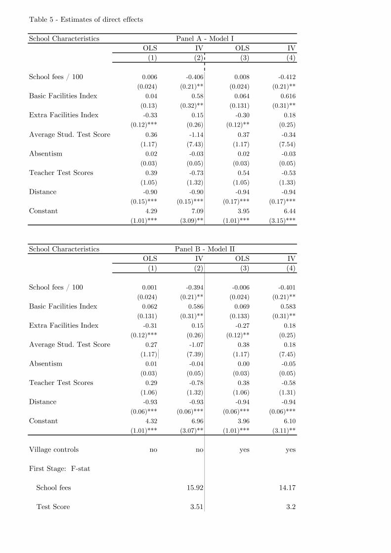
Table 5 - Estimates of direct effects


OLS IV OLS IV

(1) (2) (3) (4)

School fees / 100 0.006 -0.406 0.008 -0.412

(0.024) (0.21)** (0.024) (0.21)**

Basic Facilities Index 0.04 0.58 0.064 0.616

(0.13) (0.32)** (0.131) (0.31)**

Extra Facilities Index -0.33 0.15 -0.30 0.18

(0.12)*** (0.26) (0.12)** (0.25)

Average Stud. Test Score 0.36 -1.14 0.37 -0.34

(1.17) (7.43) (1.17) (7.54)

Absentism 0.02 -0.03 0.02 -0.03

(0.03) (0.05) (0.03) (0.05)

Teacher Test Scores 0.39 -0.73 0.54 -0.53

(1.05) (1.32) (1.05) (1.33)

Distance -0.90 -0.90 -0.94 -0.94

(0.15)*** (0.15)*** (0.17)*** (0.17)***

Constant 4.29 7.09 3.95 6.44

(1.01)*** (3.09)** (1.01)*** (3.15)***


OLS IV OLS IV

(1) (2) (3) (4)

School fees / 100 0.001 -0.394 -0.006 -0.401

(0.024) (0.21)** (0.024) (0.21)**

Basic Facilities Index 0.062 0.586 0.069 0.583

(0.131) (0.31)** (0.133) (0.31)**

Extra Facilities Index -0.31 0.15 -0.27 0.18

(0.12)*** (0.26) (0.12)** (0.25)

Average Stud. Test Score 0.27 -1.07 0.38 0.18

(1.17) (7.39) (1.17) (7.45)

Absentism 0.01 -0.04 0.00 -0.05

(0.03) (0.05) (0.03) (0.05)

Teacher Test Scores 0.29 -0.78 0.38 -0.58

(1.06) (1.32) (1.06) (1.31)

Distance -0.93 -0.93 -0.94 -0.94

(0.06)*** (0.06)*** (0.06)*** (0.06)***

Constant 4.32 6.96 3.96 6.10

(1.01)*** (3.07)** (1.01)*** (3.11)**

Village controls no no yes yes

First Stage: F-stat

School fees 15.92 14.17

Test Score 3.51 3.2

Panel A - Model I

Panel B - Model II

Table 6 - Estimates of Interaction Terms

School Characteristic

Individual/household

characteristic

School Fees / 100 Girl -0.070 -0.063 -0.050 -0.064

(0.015)*** (0.015)*** (0.008)*** (0.533)

Age -0.007 -0.009 -0.009 -0.008

(0.002)*** (0.002)*** (0.014) (0.040)

Parents Education 0.009 0.010 0.010 0.010

(0.001)*** (0.001)*** (0.000)*** (0.012)

Expenditure /100 0.002 0.002 0.002 0.002

(0.000)*** (0.001)*** (0.001)* (0.008)

Basic Facilities Index Girl 0.003 0.007 -0.009 0.006

(0.033) (0.049) (1.261) (0.151)

Age -0.017 -0.017 -0.017 -0.019

(0.000)*** (0.010)** (0.035) (0.254)

Parents Education -0.022 -0.024 -0.022 -0.025

(0.007)*** (0.007)*** (0.029) (0.064)

Expenditure /100 -0.003 -0.004 -0.003 -0.003

(0.003) (0.003)* (0.003) (0.014)

Extra Facilities Index Girl 0.022 0.119 0.101 0.112

(0.093) (0.082)* (0.420) (1.471)

Age 0.017 0.017 0.019 0.015

(0.003)*** (0.011)* (0.041) (0.716)


(0.007)* (0.005)** (0.018) (0.028)

Expenditure /100 -0.002 -0.003 -0.002 -0.002

(0.002) (0.002)* (0.005) (0.010)

Average Test Score (Stud.) Girl 0.564 0.599 0.476 0.606

(0.573) (0.270)** (1.384) (17.048)

Age -0.029 -0.040 -0.033 -0.041

(0.046) (0.008)*** (0.428) (2.390)

Parents Education -0.034 -0.038 -0.038 -0.038

(0.086) (0.038) (0.250) (0.177)

Expenditure /100 -0.006 -0.016 -0.009 -0.014

(0.022) (0.022) (0.145) (0.145)

Absentism Girl 0.007 0.017 0.016 0.022

(0.030) (0.029) (0.071) (2.420)

Age 0.001 -0.001 0.000 0.000

(0.005) (0.003) (0.019) (0.015)


(0.002)* (0.002) (0.006) (0.077)

Expenditure /100 -0.001 -0.001 -0.001 -0.001

(0.001) (0.001) (0.003) (0.029)

Teacher Test Scores Girl 0.245 0.241 0.260 0.245

(0.419) (0.419) (3.242) (3.242)

Age 0.010 -0.006 0.019 0.007

(0.026) (0.026) (0.041) (0.041)


(0.051) (0.010)*** (0.037) (0.275)

Expenditure /100 0.032 0.009 0.007 0.029

(0.014)** (0.017) (0.111) (0.209)

Distance Girl -0.449 -0.434 -0.441 -0.452

(0.190)*** (0.105)*** (0.403) (0.158)***

Age 0.000 0.015 0.013 0.010

(0.010) (0.014) (0.059) (0.353)


(0.009) (0.008) (0.080) (0.494)

Expenditure /100 0.004 -0.004 -0.004 -0.002

(0.004) (0.005) (0.004) (0.041)

Village controls no yes no yes

Panel A - Model I Panel B - Model II

Table 7 - Estimates of Interaction Terms

(unobservable household characteristics)

School Characteristic

School fees / 100 0.000 -0.002

(0.019) (0.016)

Basic Facilities Index 0.001 0.003

(0.480) (1.240)

Extra Facilities Index 0.001 -0.008

(0.682) (1.053)

Average Stud. Test Score -0.001 0.000

(0.095) (0.515)

Absentism -0.001 0.011

(0.248) (1.699)

Teacher Test Scores 0.000 0.001

(1.257) (3.281)

Distance 0.001 -0.002

(0.172) (1.209)

Village controls no yes

Model II

-2.5

-2-1

.5-1

-.5

0

Change in

mark

et

share

(perc

enta

ge p

oin

ts)

0 2000 4000 6000Current School Fee

Note: Change in school market share (percentage points) when school fee increases by 1%

Figure 1 - School Fee Elasticity

-15

-10

-50

Change in

mark

et

share

(perc

enta

ge p

oin

ts)

0 2000 4000 6000Current School Fee

Note: Change in school market share in percentage points with an increase in school fee by 100 rupees

Figure 2 - School Fee Elasticity

Estimating The Demand for School Attributes in...

Documents

Transcript of Estimating The Demand for School Attributes in...