ESTIMATING FOREST ATTRIBUTES FROM SPHERICAL IMAGES

ESTIMATING FOREST ATTRIBUTES FROM SPHERICAL IMAGES

by

Haozhou WANG

Bachelor of Ecology, Nanjing Forestry University, 2017

A Thesis Submitted in Partial Fulfillment of the Requirements for the Degree of

Master of Science in Forestry

in the Graduate Academic Unit of Faculty of Forestry and Environmental Management

Supervisor: John A. Kershaw Jr., PhD, FOREM, University of New Brunswick

Examining Board: John A. Kershaw, Jr., PhD, FOREM Jae Ogilvie, MScF, FOREM Dhirendra Shukla, PhD, TME

This thesis is accepted by the Dean of Graduate Studies

THE UNIVERSITY OF NEW BRUNSWICK

December, 2019

©Haozhou WANG, 2020

ii

Abstract

Forest attribute estimation is fundamental in forest inventory and management, but

is often time-consuming and labor intensive using traditional measurement methods. A

consumer-level spherical camera (Ricoh Theta S) which can obtain panoramic photos

from single exposures controlled by a smart phone, shows great potential to make forest

inventories more efficient. In this study, the spherical camera was used in estimating

stand basal area, canopy structural fractions, and individual tree diameters and heights.

Our results showed good correspondence (high r2 and low rMSE) between image

measured values and field measured values in most cases by linear regression. Potential

factors which may affect image estimation also were analyzed. We believe this low-cost

system could make some contributions to forest operations and more efficient forest

management.

iii

Acknowledgement

A long time and many detours were taken that brought me to this point. I believe the

project could have more depth if less time was wasted at various twists, however, without

these twists, fewer lessons would have been learned during my graduate studies. Thanks

to the UNB/NFU 3+1+1 program for providing me a chance to accomplish my graduate

studies in Canada. What is more, this project would not be accomplished without the help

of some individuals. First of all, I would like to thank Dr. John Kershaw who got me

started, patiently and responsibly guided the whole journey of this project. Specially, I

would like to thank Dr. Lavigne Mike who funded me through my toughest two seasons.

Also, Dr. Lloyd Waugh and Jae Ogilvie who served on my committee, and Goodine

Gretta who helped me with image processing and technical problems. Thank you to my

lab mates and field assistant students who helped me collect field measurement data in

Newfoundland and the Noonan Research Forest: Ting-Ru Yang, Yung-Han Hsu, Yang

Zhan, Yingbing Chen, Wushuang Li, Shun-Ying Chen, Xu Ma, and Emily Loretta

Nicholson. Also, Zizhen Gao, Rongrong Gu, Luji Xiong, Xu Gong, Tiancheng Wu in the

neighboring wood tech lab, as well as other friends in Fredericton who supported me a lot

in my local life. Finally, I would like to thank my parents, Shiquan Wang and Chunyan

Feng, for their understanding, patience, and economic support during my graduate

studies.

Funding for this project was provided in part by the National Science and

Engineering Research Council of Canada, Discovery Grants program, the Province of

Newfoundland and Labrador Centre for Forest Science and Innovation Contribution

iv

Agreement, and the New Brunswick Innovation Foundation Research Assistant’s

Initiative and Graduate Scholarships programs.

v

Table of Contents

Abstract............................................................................................................................... ii

Acknowledgement ............................................................................................................. iii

Table of Contents ................................................................................................................ v

List of Tables ................................................................................................................... viii

List of Figures ..................................................................................................................... x

List of Abbreviations ...................................................................................................... xvii

Chapter 1: General Introduction ..................................................................................... 1

1.1 Background .......................................................................................................... 1

1.2 Tree Parameters .................................................................................................... 1

1.2.1 Individual tree parameters ............................................................................. 1

1.2.2 Stand structure parameters ............................................................................ 3

1.3 Sampling Strategies for Parameters ..................................................................... 5

1.3.1 Equal probability ........................................................................................... 6

1.3.2 Variable probability ...................................................................................... 8

1.3.3 Stand basal area estimates by variable probability ....................................... 9

1.4 Remote Sensing Technologies ........................................................................... 11

1.4.1 Above canopy remote sensing .................................................................... 11

1.4.2 Below canopy remote sensing .................................................................... 13

1.5 Objectives ........................................................................................................... 14

1.6 Thesis Structure .................................................................................................. 15

1.7 References .......................................................................................................... 16

Chapter 2: Estimating Forest Basal Area from Spherical Images ................................ 32

2.1 Introduction ........................................................................................................ 32

2.2 Methods and Materials ....................................................................................... 35

2.2.1 Study sites ................................................................................................... 35

2.2.2 Data collection ............................................................................................ 35

2.2.3 Image processing software .......................................................................... 37

2.2.4 Data analysis ............................................................................................... 39

2.3 Results ................................................................................................................ 41

2.3.1 Influence of different digital sample locations ........................................... 41

2.3.2 Effects of BAF choice ................................................................................. 42

vi

2.3.3 Inter-observer consistency .......................................................................... 43

2.3.4 Understory density effects .......................................................................... 45

2.4 Discussion .......................................................................................................... 45

2.5 Conclusion .......................................................................................................... 51

2.6 Acknowledgements ............................................................................................ 52

2.7 References .......................................................................................................... 52

Chapter 3: Plant Fraction Calculation from Spherical Images by HSV Color Space .. 71

3.1 Introduction ........................................................................................................ 71

3.2 Methods and Materials ....................................................................................... 76

3.2.1 Study sites ................................................................................................... 76

3.2.2 Digital data acquisition ............................................................................... 77

3.2.3 Image processing methods .......................................................................... 78

3.2.4 Data analysis ............................................................................................... 83

3.3 Results ................................................................................................................ 87

3.3.1 Classification algorithm comparison .......................................................... 87

3.3.2 Cylindrical versus hemispherical image plant fraction estimates ............... 88

3.4 Discussion .......................................................................................................... 88

3.5 Conclusion .......................................................................................................... 92

3.6 References .......................................................................................................... 93

Chapter 4: Estimating Individual Tree Heights and DBHs from Spherical Images ... 116

4.1 Introduction ...................................................................................................... 116

4.2 Methods and materials ..................................................................................... 121

4.2.1 Study sites ................................................................................................. 121

4.2.2 Data collection .......................................................................................... 121

4.2.3 Image processing algorithms .................................................................... 124

4.2.4 Data analysis ............................................................................................. 128

4.3 Results .............................................................................................................. 130

4.3.1 Urban forest validation ............................................................................. 130

4.3.2 Field forest test .......................................................................................... 132

4.3.3 Factors contributing to potential errors ..................................................... 133

4.4 Discussion ........................................................................................................ 135

4.5 Conclusion ........................................................................................................ 138

4.6 References ........................................................................................................ 139

vii

Chapter 5: General Conclusion ................................................................................... 165

5.1 References ........................................................................................................ 169

Appendix A: Panorama2BA Software Code .................................................................. 171

gui.py .......................................................................................................................... 171

ba.py ............................................................................................................................ 190

db.py ............................................................................................................................ 190

Appendix B: Plant Fraction Calculation Code................................................................ 195

config.py (HSV Threshold) ........................................................................................ 195

Hemispherical/converse.py ......................................................................................... 195

Hemispherical/plant_fraction_hemi.py ....................................................................... 199

Hemispherical/classify_all_fisheye.py ....................................................................... 201

Cylindrical/plant_fraction_cyli.py .............................................................................. 201

Cylindrical/classify_all_cylindrical.py ....................................................................... 203

Appendix C: Individual Tree Extraction Software Code ................................................ 205

app.py .......................................................................................................................... 205

Curriculum Vitae

viii

List of Tables

Table 2.1: Average stand-level estimates (standard errors in parentheses) by trial and

treatment for the 3 early spacing trials located with western Newfoundland. 61

Table 2.2: Simple linear regression results for field basal area versus photo basal area by

digital sample point type. The linear model is FBA=b0 + b1*PBA, if PBA is

the same as FBA, then b0=0 and b1=1 ........................................................... 62

Table 3.1: Percent species composition (by basal area) across the two study sites used in

this study ....................................................................................................... 103

Table 3.2: Classification accuracy assessment results. (BC-2 = blue-channel classification

with 2 classes (sky – plant), by ImageJ, HSV-2 = HSV thresholding with two

classes, and HSV-3 = HSV thresholding with three classes (sky – wood –

foliage)) ......................................................................................................... 104

Table 3.3: Classification accuracy assessment for HSV 3 classes .................................. 105

Table 3.4: Simple linear regression results for hemispherical approach versus cylindrical

approach. The linear model is PFc = b0 + b1*PFd, if PFd is the same as PFc,

then b0=0 and b1=1 ...................................................................................... 106

Table 4.1: Simple linear regression results for angle measured from image and field. The

linear model is Y=b0+b1*X, if Image (X) is the same as Field (Y), then b0=0

and b1=1 ....................................................................................................... 147

Table 4.2: Simple linear regression results for factors measured from field and field angle

derived. The linear model is Y=b0+b1X, if field angle derived (X) is the same

as Field measured (Y), then b0=0 and b1=1 ................................................. 148

ix

Table 4.3: Simple linear regression results between image estimates and field measures.

The linear model is Y=b0+b1*X, if Image measured (X) is the same as Field

measured (Y), then b0=0 and b1=1 .............................................................. 149

Table 4.4: Summary of KS-Tests for real forest validation. Plot radii varied by spacing

treatment (Control (S00, 5.2m);1.2m (S12, 7.2m); 1.8m (S18, 10.4m); 2.4m

(S24, 15.0m); 3.0m (S30, 18.0m)) ................................................................ 150

x

List of Figures

Fig 1.1: Tools used in individual tree diameter and height measurements ....................... 28

Fig 1.2: Tools used in stand level attributes measurements .............................................. 29

Fig 1.3: Equal probability and variable probability sampling design ............................... 30

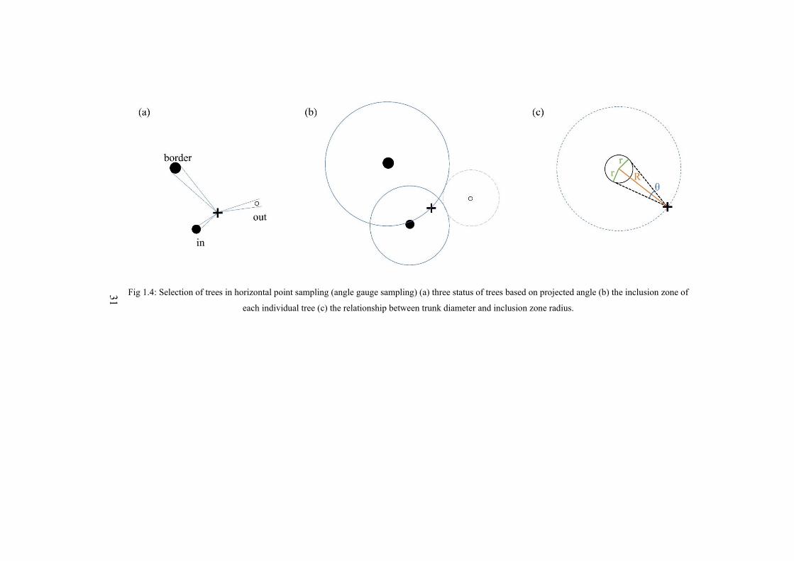
Fig 1.4: Selection of trees in horizontal point sampling (angle gauge sampling) (a) three

status of trees based on projected angle (b) the inclusion zone of each individual

tree (c) the relationship between trunk diameter and inclusion zone radius. ...... 31

Fig. 2.1: Digital data collection methods: (a) Digital sample location design for

Newfoundland (NL) and Noonan Research Forest (NRF) (Three locations were

established at the midpoint of plot radius along azimuths of 120°, 240°, and 360°

in each NL plot, while only one location was set in the center for each NRF

plot); (b) tripod and camera set up for spherical image acquisition. .................. 63

Fig. 2.2: Sample geometry. For angle count sampling: (a) overhead view showing “in”,

“border” and “out” tree (gray circles represent tree trunks); (b) the relationship

between horizontal angle (θ), tree diameter (D) and plot (inclusion zone) radius

(R). The BAF determines the fixed horizontal angle θ which was used as the

threshold to determine tree status on the spherical images. ................................ 64

Fig. 2.3: Two image processing methods: (a) Edge marking method – users click on the

edges of each tree. A reference bar (the length is based on BAF=1) is used to

guide users so that every tree does not have to be marked; the line color indicates

tree status based on desired BAF: black = “in”, gray = “out”); (b) Target count

method - a transparent reference octagon, scaled to the desired BAF is provided

xi

to mark “in” trees - “out” trees are those trees smaller than the octagon target

and are not marked. ............................................................................................. 65

Fig. 2.4: Comparisons between photo estimated basal area (PBA) and field measured

basal area (FBA) by digital sample location type (one center versus three

individuals versus mean of three individuals) and two tree marking method

(target counting (left panels) versus edge marking (right panels)). The one center

estimates (a and d) were from the Noonan Research Forest (NRF) and the three

estimates per plot (b and e) and mean of three estimates (c and f) were from the

Newfoundland (NL) spacing trials. ..................................................................... 66

Fig. 2.5: The influence of photo basal area factor (BAF) choice on the basal area

difference (field basal area – photo basal area, m2/ha) for Newfoundland (NL)

and Noonan Research Forest (NRF). The black solid line is the mean for each

location and the gray dashed line indicates perfect fit ........................................ 67

Fig. 2.6: Comparisons between field basal area and photo basal area by two marking

methods (edge marking versus target counting) among seven different users. The

locally weighted scatterplot smoothing (LOWESS) regression lines show the

trends between field measure and photo. ............................................................ 68

Fig. 2.7: Two plots with the smallest (a) and largest (b) variance among seven users by

two tree marking methods (edge marking versus target counting). PBA means

photo-based basal area and FBA means field-based basal area. The FBA of (a) is

30 m2/ha, and FBA of (b) is 55.2 m2/ha. The small dots are the tree edges that

users marked. The black small dot with connected lines means this tree is

counted as an “in” tree, while the light gray small dots means it is an “out” tree

xii

in edge marking mode. The dark gray octagon is the “in” tree marked in target

counting mode. .................................................................................................... 69

Fig. 2.8: Effects of understory density on the basal area difference (field basal area –

photo basal area, m2/ha) in the NRF plots by two marking methods (target

counting (left panels) versus edge marking (right panels)). (a) and (d) are total

understory trees, (b) and (e) are understory trees whose height smaller than 1.3

m, while (c) and (f) are those greater than 1.3 m. ............................................... 70

Fig. 3.1: The location of sites used in this study. The first site was three early spacing

trails located in western Newfoundland (NL), Canada, the second site was the

Femelschlag Research Study located on the Noonan Research Forest (NRF) in

central New Brunswick, Canada. ...................................................................... 107

Fig. 3.2: Digital data collection methods. (a) Digital sample location design for three sites

in Newfoundland (NL) and Noonan Research Forest (NRF) Study. For NL sites,

three locations were established at the midpoint of plot radius along azimuths of

360°, 120°, and 240°. For NRF, only one location center was set. (b) tripod and

spherical camera set up for spherical image acquisition at different heights

(1.6m, 2.6m, 3.6m, 4.6m). ................................................................................ 108

Fig. 3.3: The HSV thresholds for different classes. S1 is clear sky, S2 is diffused sky, S3

is cloudy sky, while F is foliage. (the remaining space is assumed to be woody

stems and branches) .......................................................................................... 109

Fig. 3.4: The workflow of two approaches to estimate plant fraction (PF) from spherical

photos. The left blue workflow is the hemispherical approach (HPF) which

converts original cylindrical images to hemispherical images first then apply

xiii

algorithms commonly used in hemispherical images. The right green one is the

cylindrical approach (CPF) which directly calculate the PF value on original

cylindrical images without image converting. .................................................. 110

Fig. 3.5: Classification accuracy assessment by error matrix. (a) is the result produced by

image classification algorithm, (b) is the result by visual inspection as true value,

(c) is a comparison error matrix generated by classified and true images. ....... 111

Fig. 3.6: Classification results comparison between HSV threshold in hemispherical

approach (HPF) and ImageJ blue channel threshold (BPF). (a) is NRF site and

(b) is NL sites .................................................................................................... 112

Fig. 3.7: Several extreme plant fraction values differences caused by overexposure and

flashed out. ........................................................................................................ 113

Fig. 3.8: Classification results for two algorithms (HSV threshold and Blue-Channel

threshold) by 7 representative image segments. (a) (b) white pure sky from

COR_R3_S18_1; (c) pure blue sky from Femel_33_11; (d) gradual change sky

from ROD_R2_S18_1; (e) (f) over exposure from Femel_29_16 and

Femel_33_13 respectively; (g) underexposure from Femel_31_13. ................ 114

Fig. 3.9: Classification results comparison by two approaches. The spherical images were

classified into 3 classes: sky (b), foliage (c), wood (d). The plant class (a) is the

sum of foliage and wood. .................................................................................. 115

Fig. 4.1: Two study sites locations in this study. ............................................................ 151

Fig. 4.2: Digital data collection methods. (a) tripod and spherical camera set up for

spherical image acquisition at two different heights (1.6m and 2.6m). (b) Digital

sample location design for urban area feasibility validation and real forest

xiv

application. For Urban Site, only one location center was set. For Forest Site,

three locations were established at the midpoint of plot radius along azimuths of

0°, 120°, and 240°. ............................................................................................ 152

Fig. 4.3: The distance, slope deviation, and tree height calculation from the side view of

spherical geometry. (a) derived the distance (R) and slope deviation (△h)

caused by terrain by key points of tree bases. (b) is the height calculation by key

points of tree tips. .............................................................................................. 153

Fig. 4.4: The DBH calculation in spherical geometry. (a) is the calculation for 1.3m

height in image. (b) is the hint about DBH boundary marking and distance to

tree center in stereo coordinates (using 1.6m digital sample height for example);

(c) is the geometry calculation for DBH. .......................................................... 154

Fig. 4.5: The graphical user interface that used to extract the key points coordinates of

individual trees for parameter calculation. The images show in this figure are

plot B with steep slope. And the yellow line shows the horizontal line (the

equator) of spherical images. ............................................................................ 155

Fig. 4.6: The angle comparison between image measured and field measured. ............. 156

Fig. 4.7: Comparisons between field measures and those derived from field measured

angles using spherical geometry: (a) comparison between radial distance (R)

derived from field angles (DerivedR) and R as measured in the field (FieldR);

(b) comparison between height derived from field angles (DerivedHT) and HT

as measured at digital sampling point (ProjectedHT); (c) comparison between

height derived from field angles (DerivedHT and HT as measured in the field at

proper place where tree tip and base were clearly visible (FieldHT). .............. 157

xv

Fig. 4.8: Radial distance comparisons between field measured and image estimates. ... 158

Fig. 4.9: Individual height (HT) comparisons between field measured and image

estimates. (a) is compared with field height measured at the digital sampling

points, (b) is compared with field height measured at proper place that can see

the tree tip clearly. ............................................................................................. 159

Fig. 4.10: DBH comparisons between field measured and image estimates (a) is

compared with projected DBH measured by caliper, (b) is compared with DBH

measured by dimeter tape. ................................................................................ 160

Fig. 4.11: Field measured (green) distributions versus image estimated (red) distributions

for DBH and HT by spacing treatment: (a) and (f) Control; (b) and (g) 1.2m

Spacing; (c) and (h) 1.8m Spacing; (d) and (i) 2.4m spacing; and (e) and (j) 3.0m

Spacing. ............................................................................................................. 161

Fig. 4.12: The residual error between field measured and image measured distances

(imageR - fieldR) under different factors (radial distance, R; tree height, HT;

diameter at breast height, DBH). The red line is the LOWESS regression and

shows the trend of errors with the factor changes. ............................................ 162

Fig. 4.13: The residual error between field measured and image measured heights

(imageHT - fieldHT) under different factors (radial distance, R; tree height, HT;

diameter at breast height, DBH). The red line is the LOWESS regression and

shows the trend of errors with the factor changes. ............................................ 163

Fig. 4.14: The residual error between field measured and image measured DBHs

(imageDBH - fieldDBH) under different factors (radial distance, R; tree height,

xvi

HT; diameter at breast height, DBH). The red line is the LOWESS regression

and shows the trend of errors with the factor changes. ..................................... 164

xvii

List of Abbreviations

AA Average accuracy BA Basal area, the cross-sectional area of tree trunk at breast height BAF Basal area factor BC Blue channel in RGB color space BPF Plant fraction by blue-channel classification algorithms CFF Foliage fraction by cylindrical approach (in Chapter 3) CPF Plant fraction by cylindrical approach (in Chapter 3) CWF Wood fraction by cylindrical approach (in Chapter 3) DBH Individual tree stem diameter at breast height (1.3m) DSP Digital sample point EVI Enhanced vegetation index FBA Field basal area GF Gap fraction GPS Global positioning system HFF Foliage fraction by hemispherical approach (in Chapter 3) HPF Plant fraction by hemispherical approach (in Chapter 3) HWF Wood fraction by hemispherical approach (in Chapter 3) HPS Horizontal point sampling HSV Hue, saturation, brightness (value) color space HT The total height of tree LAI Leaf area index LiDAR Light detection and ranging LME Linear mixed effect (models) LOWESS Locally weighted scatterplot smoothing NDVI Normalized difference vegetation index NL Newfoundland NRF Noonan Research Forest OA Overall accuracy PAi Producer’s accuracy of class i PAI Plant area index PBA Photo basal area PF Plant fraction RAW Raw image file (minimally processed data from the camera sensor) RGB Red, green, blue color space rMSE Root mean square error SAVI Soil-adjusted vegetation index SfM Structure from Motion SI The International system of units TF Tree factor or expansion factor TLS Terrestrial laser scanner UAV Unmanned aerial vehicles VPS Vertical point sampling

1

Chapter 1: General Introduction

1.1 Background

Forests are the dominant terrestrial ecosystem on Earth and account for over three

quarters of the gross primary productivity of the biosphere and about 80% of plant

biomass (Pan et al. 2013). They provide several ecosystem services including watershed

protection, soil structure maintenance, and global carbon storage (Chazdon 2008). Due to

the importance of forests, estimating complex forest conditions using easily-measured

tree attributes is critical to forest inventory and management.

1.2 Tree Parameters

1.2.1 Individual tree parameters

Individual tree attributes are of great importance, because they are often the

fundamental measures of area-based attribute estimates such as total volume and biomass

which are difficult or even impossible to measure directly. Individual tree attributes often

include age, stem diameter (cross-sectional areas), total height, merchantable height,

main stem form, and crown parameters (Kershaw et al. 2016). Typically diameter at

breast height (DBH; breast height (BH) = 1.3m) and total height (HT) are the most

common individual tree attributes measured (Avery and Burkhart 2002), and are the

fundamental parameters used in allometric equations to estimate biomass, volume, or

carbon (Lambert et al. 2005, Xing et al. 2005, Zianis et al. 2005).

The definition of tree diameter is a straight line that passes through the tree center

and meets each end of the tree bark (Kershaw et al. 2016). This attribute is important due

2

to the ability to directly measure and the ability to derive other parameters such as cross-

sectional area (basal area, BA), surface area, and trunk volume (Kershaw et al. 2016).

Though which diameters should be measured vary with different circumstance, the

diameter at breast height (1.3 m in SI units or 4.5 ft in imperial units) is widely used in

North America (Kershaw et al. 2016). Traditionally, this attribute can be easily measured

by contact dendrometers (Fig 1.1.a-d) such as diameter tape, Biltmore stick, calipers, and

sector fork (Jackson 1911, Bower and Blocker 1966, Kershaw et al. 2016). Clark et al.

(2000a) comprehensively reviewed various diameter measurement tools and their

associated accuracies. In this review, he also pointed out that although these tools are

very handy and have been widely used among researchers and forest managers, the

reliability and subjectivity effects should be taken into consideration for large-scale

inventory work.

Tree height has several definitions, including total height, bole height, merchantable

height, stump height, and so on (Kershaw et al. 2016). Total height, which is defined as

the vertical distance from the tip of tree to the ground, is commonly used. Traditionally,

total height is measured from the ground based on similar triangles or trigonometry

(Kershaw et al. 2016). Based on these principles, instruments such as the hypsometer,

clinometer, and altimeter (Fig 1.1.e-i) accompanied with a measuring tape for horizontal

distance were used in field measurement (Pardé 1955, Wesley 1956, Curtis and Bruce

1968, Iles and Fall 1988, Kershaw et al. 2016). But with the development of technology,

several advanced electronic hypsometers (Fig 1.1.j) which use laser or ultrasonic sound

waves to measure distances precisely are available with the disadvantage of a high price

(US$800-US$3000) and bulkiness (Kershaw et al. 2016).

3

1.2.2 Stand structure parameters

Stand-level attributes such as basal area per ha, volume per ha, and biomass per ha

are usually estimated by summing individual tree values and applying the appropriate

expansion factors to scale from plot to per unit area (Kershaw et al. 2016). For stand

crown and canopy measurement, attributes such as crown closure, canopy cover, and leaf

area index are often measured at the stand level rather than summarized from individual

tree measurements (Kershaw et al. 2016).

Stand basal area, defined as the sum of individual tree cross-sectional areas, is one

of the most common stand-level parameters estimated in most forest inventories (Iles

2003, Kershaw et al. 2016). Basal area is often expressed at breast height, and is an

important measure of stand density that incorporates tree size as well as number

(Kershaw et al. 2016). It is a fundamental component of volume and biomass calculations

(Iles 2003, Jenkins et al. 2003, Lambert et al. 2005, Slik et al. 2010) and is an important

stand characteristic for forest growth models (Opie 1968, Lootens et al. 2007, Weiskittel

et al. 2011). Stand basal area can be derived by summarizing the DBH of all trees in

fixed-area plots, or can be calculated using horizontal point sampling by counting the

numbers of trees that subtend a projected horizontal angle and multiplying by a constant

without measuring any DBHs (Kershaw et al. 2016). Horizonal point sampling typically

uses tools such as an angle gauge, relascope, or prism (Fig 1.2.a-c) to decide which trees

are counted. The theory of this sampling method will be discussed in Section 1.3.2.

There are several canopy attributes such as gap fraction, canopy cover, canopy

closure, canopy openness, and so on. These attributes are similar but slightly different

concepts that need to be clarified (Gonsamo et al. 2013).

4

Gap fraction (GF, or P0), defined as “the area fraction of open sky not obstructed by

canopy elements over the limited area defined by specific view zenith (θ) and azimuth

(Φ) angles” (Gonsamo et al. 2013), The key point of the GF definition is the limited area

fraction defined by specific view angles. Commonly, the GF or P0 should include two

subscripts: GF (θ, Φ) or P0 (θ, Φ). When the azimuth angle is not given, GF (θ) or P0 (θ)

represent the gap proportion in a narrow ring area at that zenith angle (Jonckheere et al.

2005, Pekin and MacFarlane 2009).

Canopy cover is the proportion of canopy elements vertically projected onto the

ground (Gonsamo et al. 2013). This measurement is easy to measure from a vertical

direction, and is commonly measured using satellite, airborne, or unmanned aerial vehicle

(UAV) images.

Canopy openness is defined as “the area fraction of the sky hemisphere (180°) that

is unobstructed by canopy elements when viewed from a single point” (Gonsamo et al.

2013). The key point of canopy openness is the full sky hemisphere (180°). Canopy

openness can be simply calculated from the sky pixels versus total pixel numbers in

classified binary images.

Canopy closure, defined as the complement of canopy openness (1 – canopy

openness), ideally it is expressed using the whole hemisphere, however, closure

measurements are often restricted by selected zenith angles because horizon gaps and

canopy elements are hard to measure (Gonsamo et al. 2013). Canopy closure often is the

same definition as plant fraction, which is used in this study, and a restricted zenith angle

of 57.5° is often used. Lemmon (1956, 1957) first developed a method to measure plant

fraction using a spherical densiometer (Fig 1.2.d) which is a curved mirror with a grid,

5

and counting the number of grids containing plants divided by the total grid number.

Photographic techniques with high-quality digital images provide a much more accurate

and repeatable measure than traditional grid counting (Kershaw et al. 2016). This image-

based method is sensitive to thresholding which separates the image pixels into sky and

other components.

Leaf area index (LAI) is the total foliage area (one-sided projection area) in a unit

area (Kershaw et al. 2016), the units are 𝑚 ⋅ 𝑚 or 𝑚 ⋅ ℎ𝑎 . This parameter shows a

strong linear relationship with stem wood and total biomass production (Waring et al.

1981, Oren et al. 1987, Vose and Allen 1988). The direct method to estimate LAI

requires destructive sampling: felling individual trees and weighing the foliage in lab

(Kershaw et al. 2016). This method is not only labor intensive, but also has effects on the

remaining stand. Indirect methods such as allometric regression relationships, litterfall

traps (Fig 1.2.e), and indirect noncontact methods have theoretical, practical, or

methodological challenges (Larsen and Kershaw 1990, Weiss et al. 2004, Jonckheere et

al. 2004). Alternatively, hemispherical photographic methods (Fig 1.2.f) are widely used

in forest LAI estimates (MacFarlane et al. 2007a, Liu et al. 2013, Fournier and Hall

2017). These methods employ simple models of forest canopy radiation transfer, along

with image processing and the relationship between gap fraction and zenith angle to

estimate LAI (Rich 1990, Weiss et al. 2004).

1.3 Sampling Strategies for Parameters

Measuring the attributes of all individual trees in a stand or forest area should be the

most accurate method to evaluate forest conditions, ideally. However, obviously, it is

6

quite labor intensive and time consuming, also it is not applicable for large scale forest

inventories. The most common practice is using sample plots, which are defined as the

units for recording information and measurements (Kershaw et al. 2016). Basic sampling

strategies can be divided into two main categories: equal probability and variable

probability.

1.3.1 Equal probability

The most common sample plot has been a unit of fixed area for many years, and

these fixed-area sampling units are often small areas of square, rectangular, circular, or

triangular shape (Kershaw et al. 2016). A plot center is set in a forest, and based on this

center, a boundary of fixed-area, shape, and orientation determined. Each tree meeting

some defined height or diameter criteria included within the boundary is selected and

measured.

Alternatively, each tree can be thought to have its own inclusion zone which is the

same size, shape, and orientation as the fixed-area boundary, just centered on each tree. A

sample point (plot center) is set in the forest, and those trees whose inclusion zones

include the plot center are selected and measured (Fig 1.3.a&b). In this procedure, the

probability of selection is the same for all individual trees because their inclusion zones

are all the same size (Kershaw et al. 2016), and therefore, their probabilities of selection

are equal.

Circular plots, which use a radius as a single dimension to define the boundary,

have been widely used (Kershaw et al. 2016). In this plot type, the inclusion zone of each

individual tree has the same radius as the plot radius (Fig 1.3.a). The main advantages of

7

circular plots are: 1) The length of boundary is the minimum of all shapes with the same

area. It implies fewer decisions to judge trees near the boundary. 2) Unlike rectangle or

strip plots, circular plots have no predetermined orientation. and 3) They are the simplest

for correcting slopover bias, which caused by the inclusion zone of one tree partly falls

outside the plot center. The main disadvantage is the difficulties associated with carefully

determining distances from trees to plot center without the assistance of modern

ultrasonic or laser distance measuring tools (Kershaw et al. 2016). Unlike circular plots,

square or rectangular plots are much easier to decide in or out due to the straight-line

boundary, also these straight boundaries can be easily marked by compass and tape

(Kershaw et al. 2016). But laying out the plot corners and boundaries carefully and the

orientation effects should be taken into consideration when analyzing bias (Kershaw et al.

2016).

The fixed-area plot also has limitations. Normally, in the east coast of the North

America, there are many more small trees than large ones in natural forests. Due to the

equal probability, there tends to be many small trees selected in this sampling method.

However, compared with large trees, when measuring volume, biomass, or carbon

storage, small trees are less proportionally of lower influence or consequence, but are

measured many more times than large trees (Kershaw et al. 2016). To solve this problem,

different sizes of plots for different sized vegetation can be used. For example, Van Den

Meersschaut and Vandekerkhove (2000) used four concentric circular plots with 4

different areas to measure: seedlings (16 m2), shrubs (64 m2), living trees (255 m2), dead

trees (1018 m2), and lesser vegetation and lying deadwood (16 m×16 m). While this is

still considered fixed area plot sampling, it is really an intermediate step between equal

8

probability sampling and variable probability sampling (Section 1.3.2) and can be quite

cumbersome to implement in the field.

1.3.2 Variable probability

While using concentric plots is one method to solve the problem of oversampling

certain classes of vegetation, using a sampling procedure in which the probability of

selecting a tree depends on some tree character (e.g. DBH or HT) is also possible

(Kershaw et al. 2016). In this situation, larger trees have larger inclusion zones while

smaller trees have smaller zones (Fig 1.3.c), which means, the probability of selecting a

tree is proportional to its size (Kershaw et al. 2016). Variable probability is a very

efficient sampling scheme; however, because there is high variance in counts of trees

between points, sample sizes are often much higher than when using fixed area plots (Iles

2003, Kershaw et al. 2016, Yang et al. 2017). As a result, various subsampling schemes

have been developed to reduce the point and tree measurements (Grosenbaugh 1963a,

Iles 2003, Marshall et al. 2004, Yang et al. 2017). Variable probability selection can be

applied to trees, sample points, and even stands (Kershaw et al. 2016); however, one of

the limitations of variable probability sampling is identification of an appropriate

covariate for selection (Hsu et al. In Review).

Horizontal Point Sampling, is the most used application of variable probability

sampling and was originally developed by Bitterlich (1947). It is also called angle count

sampling because an angle is used to select trees proportional to their basal area

(Bitterlich 1947, 1984). In this method, the observer occupies the point (plot center) and a

horizontal angle (often created by tools shown in Fig 1.2.a-c) is projected towards each

9

tree at DBH level (Fig 1.4.a). All trees that are as large as or larger than the projected

horizontal angles are counted.

1.3.3 Stand basal area estimates by variable probability

In most forest inventory data analyses, measurements are summarized and divided

by the total plot size to express values on a per unit area basis (Kershaw et al. 2016). The

ratio of each selected tree scaled to per unit area measurement is called the tree factor or

expansion factor (Kershaw et al. 2016). For each tree:

𝑇𝐹𝑈𝑛𝑖𝑡 𝐴𝑟𝑒𝑎

𝐼𝑛𝑐𝑙𝑢𝑠𝑖𝑜𝑛 𝑧𝑜𝑛𝑒 𝑎𝑟𝑒𝑎 (1.1)

where TFi is the tree factor of sample tree i, unit area is 10000 m2, inclusion zone areai is

the inclusion zone area of sample tree i in the same units as Unit Area.

Tree factor can then be used to expand specific tree attributes (Attribute Factor, XFi)

to stand or forest level attributes by simply multiplying the value of that attributes (Xi) by

tree factor (TFi):

𝑋𝐹 𝑋 ∙ 𝑇𝐹 (1.2)

The stand attribute value equals the sum of all selected trees:

𝑋 𝑋𝐹 𝑋 ∙ 𝑇𝐹 (1.3)

e.g. Stand Basal Area

𝐵𝐴 𝐵𝐴𝐹 𝐵𝐴 ∙ 𝑇𝐹 (1.4)

Combined with Eq. (1.1):

10

𝐵𝐴 𝐵𝐴 ∙𝑈𝑛𝑖𝑡 𝐴𝑟𝑒𝑎

𝐼𝑛𝑐𝑙𝑢𝑠𝑖𝑜𝑛 𝑍𝑜𝑛𝑒 𝐴𝑟𝑒𝑎

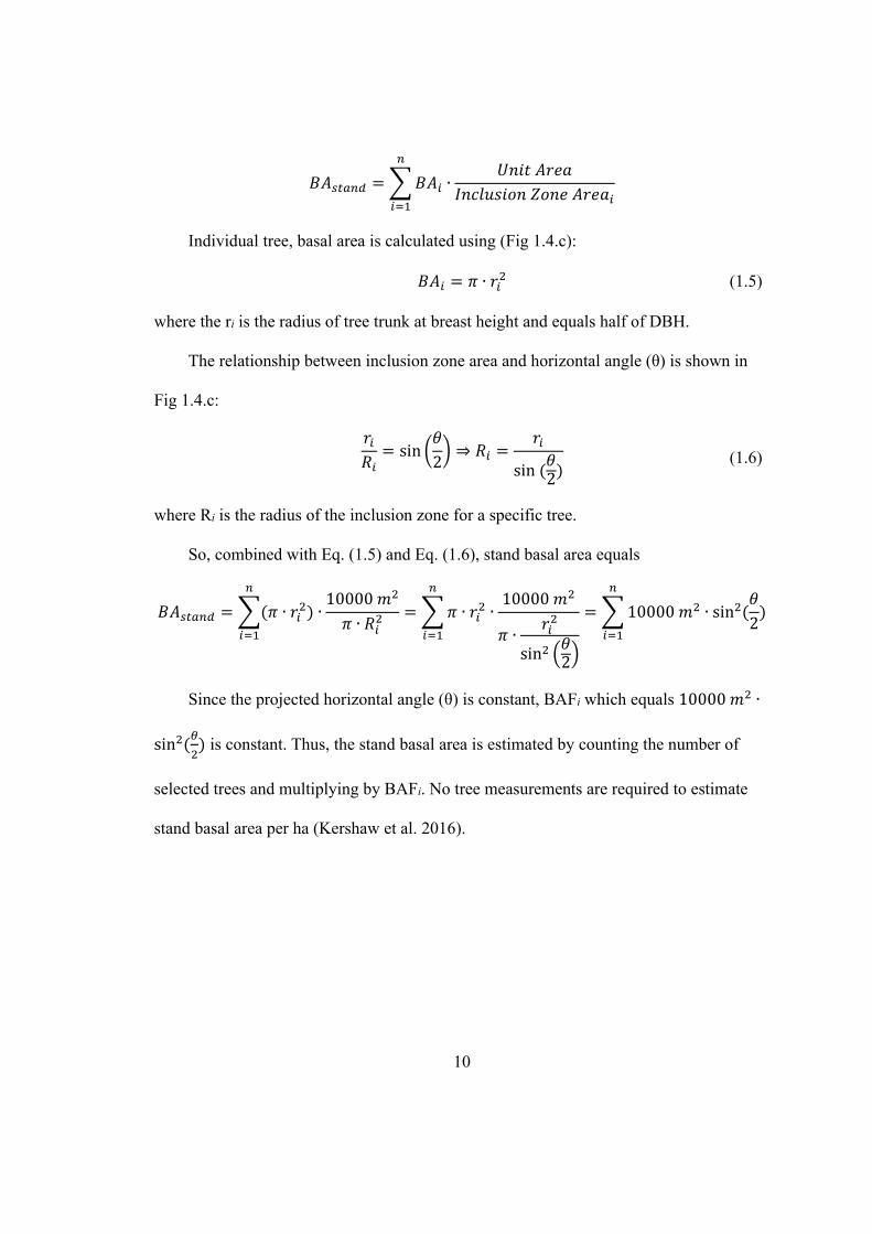
Individual tree, basal area is calculated using (Fig 1.4.c):

𝐵𝐴 𝜋 ∙ 𝑟 (1.5)

where the ri is the radius of tree trunk at breast height and equals half of DBH.

The relationship between inclusion zone area and horizontal angle (θ) is shown in

Fig 1.4.c:

𝑟𝑅

sin𝜃2

⇒ 𝑅𝑟

sin 𝜃2

(1.6)

where Ri is the radius of the inclusion zone for a specific tree.

So, combined with Eq. (1.5) and Eq. (1.6), stand basal area equals

𝐵𝐴 𝜋 ∙ 𝑟 ∙10000 𝑚𝜋 ∙ 𝑅

𝜋 ∙ 𝑟 ∙10000 𝑚

𝜋 ∙𝑟

sin𝜃2

10000 𝑚 ∙ sin𝜃2

Since the projected horizontal angle (θ) is constant, BAFi which equals 10000 𝑚 ∙

sin is constant. Thus, the stand basal area is estimated by counting the number of

selected trees and multiplying by BAFi. No tree measurements are required to estimate

stand basal area per ha (Kershaw et al. 2016).

11

1.4 Remote Sensing Technologies

1.4.1 Above canopy remote sensing

Above canopy remote sensing techniques, e.g. satellite, manned aircraft, and

unmanned aerial vehicles (UAV), are applied in forest inventory to save time and

workloads for large-scale investigations.

Satellite remote sensing is a mature technology for large scale investigation, it can

be applied for estimating biomass, leaf area, land-cover classification, and deforestation

monitoring (Tucker et al. 1985, Running et al. 1986, Skole and Tucker 1993, Lu 2006,

Jin et al. 2014). The most common method for these applications is using different

vegetation indices such as normalized difference vegetation index (NDVI), soil-adjusted

vegetation index (SAVI), enhanced vegetation index (EVI), and so on to represent plant

or environmental conditions (Major et al. 1990, Nagler et al. 2005). However, limited by

the low spatial resolution, cloud contamination, and overpass period, it is difficult for

conventional satellite remote sensing techniques to estimate individual tree information

which match with the detailed data measured during ground investigations (Turner et al.

2012).

Airborne remote sensing has been developed for many years (Reeves 1936, Colwell

1964). Airborne images are no longer limited to sensors in the visible spectrum, but also

can use infrared, laser (LiDAR), ultrasonic (radar), and even hyperspectral (Kasischke et

al. 1997, Asner et al. 2007, Smith et al. 2010). Several attributes such as canopy height

(Paine and Kiser 2012), species detection (Junttila and Kauranne 2012), canopy diversity

(Asner and Martin 2009, Asner et al. 2017), and above ground biomass (Lefsky et al.

12

2002, Meyer et al. 2013, Hayashi et al. 2015) can be estimated using this technology.

However, manned aircraft is limited by flight route control in some areas and the sensors

often have a very high investment cost, thus high costs for airborne imaging.

This big challenge is partially resolved by unmanned aerial vehicle (UAV) remote

sensing, which is an emerging tool to provide timely, lower-cost, and high resolution

means of investigation (Anderson and Gaston 2013). Several studies demonstrate the

possibility of using high resolution UAV images to extract individual tree heights and

crown coverages by structure from motion (SfM) techniques (Turner et al. 2012, Dandois

and Ellis 2013, Wallace et al. 2016). Also the vegetation structure and functional

properties can be extracted to explore biodiversity (Getzin et al. 2011, Hoffmann et al.

2016). However, many of these approaches require high-performance-computers for

indoor 3D point cloud reconstruction and data analysis, driving up the costs and time

required to complete inventories. The canopy makes extracting tree trunk attributes hard

when using visible spectrum sensors. Though radio and laser sensor techniques make

penetration of canopies easier (Wallace et al. 2016, Asner et al. 2017), the high prices of

these sensors limit wide spread use. Also, the scale at which a UAV sample can be

efficiently processed is generally too small for a woodlot-scale inventory.

Above canopy remote sensing has saved a large amount of labor and makes large

scale forest investigations possible. However, collecting under canopy forest attributes

data for validation cannot be avoided.

13

1.4.2 Below canopy remote sensing

For under canopy data collection, there are also some novel indirect optical remote

sensing tools. Some of the simpler tools were introduced in Section 1.2, some other self-

made and minority instruments such as TRAC and MVI (for PAI/LAI measurement),

DEMON (for beam transmission), spherical densiometer (for forest canopy parameters),

and Moosehorn (for crown closure) are seldomly used in practice (Seidel et al. 2011).

The most popular optical methods includes hemispherical (fisheye) cameras (MacFarlane

et al. 2007b, Jonckheere et al. 2009, Brandão et al. 2016), laser scanners (Lefsky et al.

2002, Seidel et al. 2012, Hayashi et al. 2015), and digital cameras (Lati et al. 2011,

Maynard et al. 2014, Inoue et al. 2015).

Hemispherical photographs have been used to estimate crown and canopy

parameters, such as gap fraction, foliage cover, and leaf area index for many years

(Demarez et al. 2008, Zhao et al. 2012). Though many software and algorithms have been

developed to analyze fisheye images (van Gardingen et al. 1999, Lang and Yueqin 1986,

Montes et al. 2007, Seidel et al. 2011), the high price of traditional hemispherical

cameras make consumer-grade digital cameras more and more popular for different

aspects of forest measuring (Frazer et al. 2001).

Terrestrial (ground-based) laser scanner (TLS) is an optical method which has the

ability to record 3D point cloud information of the forest structure. Several studies have

used this novel tool to estimate biomass and canopy metrics (Hilker et al. 2010,

Holopainen et al. 2011, Wallace et al. 2017). Directly using the point cloud 3D

information to calculate biomass by counting plant voxel volume is another approach

(Seidel et al. 2012). However, the high price of laser scanners (50 to 80 times the price of

14

a fisheye camera) (Seidel et al. 2011) accompanied by the long scanning times,

difficulties in analyzing point clouds, and high computer hardware performance

requirements significantly limits wide spread use.

Using consumer-grade digital cameras to extract tree attributes has been developed

over decades including measuring upper stem diameters (Grosenbaugh 1963b), heights

(Clark et al. 2000b), and even generating 3D stem models (Larsen 2006, Mokroš et al.

2018). These studies pay more attention to photographing single trees, which is not so

useful for estimating attributes of a large cluster of trees (Perng et al. 2018). Merging 360

degrees photos into panoramic images to get cluster attributes such as basal area is a

method reported by many researchers (Fastie 2010, Dick et al. 2010), but it only contains

horizontal information and sloped terrain makes the center of image not exactly breast

height (Perng et al. 2018).

The new 360° spherical cameras offer an inexpensive option for obtaining inventory

covariates and potentially obtaining direct stand and tree measurements. The compact

size of a spherical camera makes it an easy-to-use tool in the forest and can be moved

through the canopy to obtain structural estimates more easily than traditional fisheye

cameras and other digital cameras.

1.5 Objectives

This project has three main objectives. The first one will use the horizontal part of

spherical images to extract stand basal area. The second part will extract forest canopy

attributes in the vertical projection of spherical images. The last objectives will be to

15

extract individual tree attributes from two spherical images taken at different heights. The

specific objectives are as follows:

1. Using spherical images for image-based angle count sampling to estimate stand

basal area and analyze effects of potential vegetation and stand structure factors that

might limit generalization of this techinique.

2. Developing a novel HSV classification threshold to classify transformed or

original spherical images and to estimates plant fractions, stem fractions, foliage

fractions, etc. and compare the results with traditional fisheye classification algorithm

(blue channel classification).

3. Using paired spherical images at two different heights, to extract individual tree

DBH and height; the results will be compared with field measurements obtained in an

urban setting and across an early spacing trial for a real forest comparison.

A framework that enables using spherical images to extract common forest attributes

will be developed in this project. The outcomes include several applications for Microsoft

windows for each objective respectively. This framework will provide the opportunity to

increase the efficiency in the field, reduce measurement errors and ensure data

consistency in long-term investigations.

1.6 Thesis Structure

The structure of this thesis is around five chapters to cover the objectives mentioned

above. This chapter (Chapter 1) is a general introduction chapter. Chapter 2, Estimating

Forest Basal Area from Spherical Images demonstrates how spherical images can be

used to conduct horizontal point sampling for stand basal area attributes (Chapter 2 is

16

accepted for publication in Mathematical and Computational Sciences in Forestry and

Natural Resources). Chapter 3, Plant Fraction Calculation from Spherical Images by

HSV Color Space demonstrates how spherical images can be used to estimate fisheye

camera attributes in an automatic way. Chapter 4, Estimating Individual Tree Diameters

and Heights with Spherical Images demonstrates how spherical images can be used to

extract individual tree attributes. The concluding Chapter 5 summarizes the results of this

project and future developments to extend the project direction.

1.7 References

Anderson, K., and K. J. Gaston. 2013. Lightweight unmanned aerial vehicles will

revolutionize spatial ecology. Frontiers in Ecology and the Environment 11:138–

146.

Asner, G. P., D. E. Knapp, T. Kennedy-Bowdoin, M. O. Jones, R. E. Martin, J. Boardma,

and C. B. Field. 2007. Carnegie Airborne Observatory: in-flight fusion of

hyperspectral imaging and waveform light detection and ranging for three-

dimensional studies of ecosystems. Journal of Applied Remote Sensing

1(1):013536.

Asner, G. P., and R. E. Martin. 2009. Airborne spectranomics: mapping canopy chemical

and taxonomic diversity in tropical forests. Frontiers in Ecology and the

Environment 7:269–276.

Asner, G. P., R. E. Martin, D. E. Knapp, R. Tupayachi, C. B. Anderson, F. Sinca, N. R.

Vaughn, and W. Llactayo. 2017. Airborne laser-guided imaging spectroscopy to

map forest trait diversity and guide conservation. Science 355:385–389.

17

Avery, T. E., and H. E. Burkhart. 2002. Forest measurements. Fifth. McGraw-Hill, New

York.

Bitterlich, W. 1947. Die winkelzählmessung (Measurement of basal area per hectare by

means of angle measurement.). Allgemeine Forst- und Holzwirtschaftliche

Zeitung 58:94–96.

Bitterlich, W. 1984. The relascope idea: Relative measurements in forestry. First. CAB

International, Slough, England.

Bower, D. R., and W. W. Blocker. 1966. Accuracy of bands and tape for measuring

diameter increments. Journal of Forestry 64:21–22.

Brandão, Z. N., J. H. Zonta, Z. N. Brandão, and J. H. Zonta. 2016. Hemispherical

photography to estimate biophysical variables of cotton. Revista Brasileira de

Engenharia Agrícola e Ambiental 20:789–794.

Chazdon, R. L. 2008. Beyond Deforestation: Restoring Forests and Ecosystem Services

on Degraded Lands. Science 320:1458–1460.

Clark, N. A., R. H. Wynne, and D. L. Schmoldt. 2000a. A review of past research on

dendrometers. Forest Science 46:570–576.

Clark, N. A., R. H. Wynne, D. L. Schmoldt, and M. Winn. 2000b. An assessment of the

utility of a non-metric digital camera for measuring standing trees. Computers and

Electronics in Agriculture 28:151–169.

Colwell, R. N. 1964. Aerial Photography - a Valuable Sensor for the ScientistT.

American Scientist 52:17–49.

Curtis, R. O., and D. Bruce. 1968. Tree heights without a tape. Journal of Forestry 66:60–

61.

18

Dandois, J. P., and E. C. Ellis. 2013. High spatial resolution three-dimensional mapping

of vegetation spectral dynamics using computer vision. Remote Sensing of

Environment 136:259–276.

Demarez, V., S. Duthoit, F. Baret, M. Weiss, and G. Dedieu. 2008. Estimation of leaf

area and clumping indexes of crops with hemispherical photographs. Agricultural

and Forest Meteorology 148:644–655.

Dick, A. R., J. A. Kershaw, and D. A. MacLean. 2010. Spatial Tree Mapping Using

Photography. Northern Journal of Applied Forestry 27:68–74.

Fastie, C. L. 2010. Estimating stand basal area from forest panoramas. Proceedings of the

Fine International Conference on Gigapixel Imaging for Science. Carnegie

Mellon University, Pittsburg, PA. 4(8).

Fournier, R. A., and R. J. Hall, editors. 2017. Hemispherical Photography in Forest

Science: Theory, Methods, Applications. Springer Netherlands.

Frazer, G. W., R. A. Fournier, J. A. Trofymow, and R. J. Hall. 2001. A comparison of

digital and film fisheye photography for analysis of forest canopy structure and

gap light transmission. Agricultural and Forest Meteorology 109:249–263.

van Gardingen, P. R., G. E. Jackson, S. Hernandez-Daumas, G. Russell, and L. Sharp.

1999. Leaf area index estimates obtained for clumped canopies using

hemispherical photography. Agricultural and Forest Meteorology 94:243–257.

Getzin, S., K. Wiegand, and I. Schöning. 2011. Assessing biodiversity in forests using

very high-resolution images and unmanned aerial vehicles. Methods in Ecology

and Evolution 3:397–404.

19

Gonsamo, A., P. D’odorico, and P. Pellikka. 2013. Measuring fractional forest canopy

element cover and openness – definitions and methodologies revisited. Oikos

122:1283–1291.

Grosenbaugh, L. R. 1963a. Some suggestions for better sample–tree measurement.

Proceedings of the 1963 Society of American Foresters National Convention.

Society of American Foresters. pp 36–42.

Grosenbaugh, L. R. 1963b. Optical dendrometers for out-of-reach diameters: A

conspectus and some new theory. Forest Science Monographs 4(48).

Hayashi, R., J. A. Kershaw Jr., and A. R. Weiskittel. 2015. Evaluation of alternative

methods for using LiDAR to predict aboveground biomass in mixed species and

structurally complex forests in northeastern North America. Mathematical and

Computational Forestry and Natural Resources Sciences 7:49–65.

Hilker, T., M. van Leeuwen, N. C. Coops, M. A. Wulder, G. Newnham, D. L. B. Jupp,

and D. S. Culvenor. 2010. Comparing canopy metrics derived from terrestrial and

airborne laser scanning in a Douglas-fir dominated forest stand. Trees, Structure

and Function 24:819–832.

Hoffmann, H., R. Jensen, A. Thomsen, H. Nieto, J. Rasmussen, and T. Friborg. 2016.

Crop water stress maps for an entire growing season from visible and thermal

UAV imagery. Biogeosciences 13:6545–6563.

Holopainen, M., M. Vastaranta, V. Kankare, M. Räty, M. Vaaja, X. Liang, X. Yu, J.

Hyyppä, H. Hyyppä, R. Viitala, and S. Kaasalainen. 2011. Biomass Estimation of

Individual Trees Using STEM and Crown Diameter Tls Measurements. ISPRS -

20

International Archives of the Photogrammetry, Remote Sensing and Spatial

Information Sciences 3812:91–95.

Hsu, Y.-H., T.-R. Yang, and Y. Chen. In Review. Sampling to correct LiDAR-assisted

forest inventories. Forest Science.

Iles, K. 2003. A sampler of inventory topics. 2nd edition. Kim Iles and Associates,

Nanaimo, BC.

Iles, K., and M. Fall. 1988. Can an angle gauge really evaluate “borderline trees”

accurately in variable plot sampling? Canadian Journal of Forest Research

18:776–783.

Inoue, T., S. Nagai, H. Kobayashi, and H. Koizumi. 2015. Utilization of ground-based

digital photography for the evaluation of seasonal changes in the aboveground

green biomass and foliage phenology in a grassland ecosystem. Ecological

Informatics 25:1–9.

Jackson, A. 1911. The Biltmore stick and its use on national forests. Journal of Forestry

9:406–411.

Jenkins, J. C., D. C. Chojnacky, L. S. Heath, and R. A. Birdsey. 2003. National scale

biomass estimators for United States tree species. Forest Science 49:12–35.

Jin, Y., X. Yang, J. Qiu, J. Li, T. Gao, Q. Wu, F. Zhao, H. Ma, H. Yu, and B. Xu. 2014.

Remote Sensing-Based Biomass Estimation and Its Spatio-Temporal Variations in

Temperate Grassland, Northern China. Remote Sensing 6:1496–1513.

Jonckheere, I., L. Comita, J. Thompson, J. Zimmerman, M. Uriarte, and P. Coppin. 2009.

Exploration of in-situ light and biomass estimation by digital hemispherical

photography in tropical forests. 11, Page 12447.

21

Jonckheere, I., S. Fleck, K. Nackaerts, B. Muys, P. Coppin, M. Weiss, and F. Baret.

2004. Review of methods for in situ leaf area index determination: Part I.

Theories, sensors and hemispherical photography. Agricultural and Forest

Meteorology 121:19–35.

Jonckheere, I. G. C., B. Muys, and P. R. Coppin. 2005. Derivative analysis for in situ

high dynamic range hemispherical photography and its application in forest

stands. IEEE Geoscience and Remote Sensing Letters 2:296–300.

Junttila, V., and T. Kauranne. 2012. Evaluating the robustness of plot databases in

species-specific light detection and ranging-based forest inventory. Forest Science

58:311–325.

Kasischke, E. S., J. M. Melack, and M. C. Dobson. 1997. The use of imaging radars for

ecological applications—A review. Remote Sensing of Environment 59:141–156.

Kershaw, J. A., Jr., M. J. Ducey, T. W. Beers, and B. Husch. 2016. Forest Mensuration.

5th edition. Wiley/Blackwell, Hobokin, NJ.

Lambert, M.-C., C.-H. Ung, and F. Raulier. 2005. Canadian national tree aboveground

biomass equations. Canadian Journal of Forest Research 35:1996–2018.

Lang, A. R. G., and X. Yueqin. 1986. Estimation of leaf area index from transmission of

direct sunlight in discontinuous canopies. Agricultural and Forest Meteorology

37:229–243.

Larsen, D. R., and J. A. Kershaw Jr. 1990. The measurement of leaf area. Techniques in

Forest Tree Ecophysiology. Lassoie, J. and T. Hinkley (eds.). CRC Press, Boca

Raton, FL. pp. 465–475.

22

Larsen, D. R. 2006. Development of a photogrammetric method of measuring tree taper

outside bark. Gen. Tech. Rep. SRS-92. Asheville, NC: U.S. Department of

Agriculture, Forest Service, Southern Research Station. pp. 347-350.

Lati, R. N., S. Filin, and H. Eizenberg. 2011. Robust Methods for Measurement of Leaf-

Cover Area and Biomass from Image Data. Weed Science 59:276–284.

Lefsky, M. A., W. B. Cohen, D. J. Harding, G. G. Parker, S. A. Acker, and S. T. Gower.

2002. Lidar remote sensing of above-ground biomass in three biomes. Global

Ecology and Biogeography 11:393–399.

Lemmon, P. E. 1956. A spherical densiometer for estimating forest overstory density.

Forest Science 2:314–320.

Lemmon, P. E. 1957. A new instrument for measuring over-story density. Journal of

Forestry 55:667–669.

Liu, C., S. Kang, F. Li, S. Li, and T. Du. 2013. Canopy leaf area index for apple tree

using hemispherical photography in arid region. Scientia Horticulturae 164:610–

615.

Lootens, J. R., D. R. Larsen, and S. R. . Shifley. 2007. Height-diameter equations for 12

upland species in the Missouri Ozark Highlands. Northern Journal of Applied

Forestry 24:1149–152.

Lu, D. 2006. The potential and challenge of remote sensing‐based biomass estimation.

International Journal of Remote Sensing 27:1297–1328.

MacFarlane, C., S. K. Arndt, S. J. Livesley, A. C. Edgar, D. A. White, M. A. Adams, and

D. Eamus. 2007a. Estimation of leaf area index in eucalypt forest with vertical

23

foliage, using cover and fullframe fisheye photography. Forest Ecology and

Management 242:756–763.

MacFarlane, C., A. Grigg, and C. Evangelista. 2007b. Estimating forest leaf area using

cover and fullframe fisheye photography: Thinking inside the circle. Agricultural


Major, D. J., F. Baret, and G. Guyot. 1990. A ratio vegetation index adjusted for soil

brightness. International Journal of Remote Sensing 11:727–740.

Marshall, D. D., K. Iles, and J. F. Bell. 2004. Using a large-angle gauge to select trees for

measurement in variable plot sampling. Canadian Journal of Forest Research

34:840–845.

Maynard, D. S., M. J. Ducey, R. G. Congalton, J. Kershaw, and J. Hartter. 2014. Vertical

point sampling with a digital camera: Slope correction and field evaluation.

Computers and Electronics in Agriculture 100:131–138.

Meyer, V., S. S. Saatchi, J. Chave, J. Dalling, S. Bohlman, G. A. Fricker, C. Robinson,

and M. Neumann. 2013. Detecting tropical forest biomass dynamics from

repeated airborne Lidar measurements. Biogeosciences 10:5421–5438.

Mokroš, M., J. Výbošťok, J. Tomaštík, A. Grznárová, P. Valent, M. Slavík, and J.

Merganič. 2018. High Precision Individual Tree Diameter and Perimeter

Estimation from Close-Range Photogrammetry. Forests 9(696).

Montes, F., P. Pita, A. Rubio, and I. Cañellas. 2007. Leaf area index estimation in

mountain even-aged Pinus silvestris L. stands from hemispherical photographs.

Agricultural and Forest Meteorology 145:215–228.

24

Nagler, P. L., R. L. Scott, C. Westenburg, J. R. Cleverly, E. P. Glenn, and A. R. Huete.

2005. Evapotranspiration on western U.S. rivers estimated using the Enhanced

Vegetation Index from MODIS and data from eddy covariance and Bowen ratio

flux towers. Remote Sensing of Environment 97:337–351.

Opie, J. E. 1968. Predictability of Individual Tree Growth Using Various Definitions of

Competing Basal Area. Forest Science 14:314–323.

Oren, R., R. H. Waring, S. G. Stafford, and J. W. Barrett. 1987. Twenty-four years of

ponderosa pine growth in relation to canopy leaf area and understory competition.


Paine, D. P., and J. D. Kiser. 2012. Aerial photography and image interpretation. 3rd

edition. Wiley, New York.

Pan, Y., R. A. Birdsey, O. L. Phillips, and R. B. Jackson. 2013. The Structure,

Distribution, and Biomass of the World’s Forests. Annual Review of Ecology,

Evolution, and Systematics 44:593–622.

Pardé, J. 1955. Le mouvement forestier à l’étranger. Un dendromètre pratique : le

Dendromètre Blume-Leiss (The forest movement abroad. A practical

dendrometer: the dendrometer Blume-Leiss). Revue Forestière Française 7:207–

210.

Pekin, B., and C. MacFarlane. 2009. Measurement of Crown Cover and Leaf Area Index

Using Digital Cover Photography and Its Application to Remote Sensing. Remote

Sensing 1:1298–1320.

25

Perng, B.-H., T. Y. Lam, and M.-K. Lu. 2018. Stereoscopic imaging with spherical

panoramas for measuring tree distance and diameter under forest canopies.

Forestry: An International Journal of Forest Research 91:662–673.

Rich, P. M. 1990. Characterizing plant canopies with hemispherical photographs. Remote

Sensing Reviews 5:13–29.

Reeves, D. M. 1936. Aerial Photography and Archaeology. American Antiquity 2:102–

107.

Running, S. W., D. L. Peterson, M. A. Spanner, and K. B. Teuber. 1986. Remote sensing

of coniferous forest leaf area. Ecology 67:273–276.

Seidel, D., S. Fleck, and C. Leuschner. 2012. Analyzing forest canopies with ground-

based laser scanning: A comparison with hemispherical photography. Agricultural

and Forest Meteorology 154–155:1–8.

Seidel, D., S. Fleck, C. Leuschner, and T. Hammett. 2011. Review of ground-based

methods to measure the distribution of biomass in forest canopies. Annals of


Skole, D., and C. Tucker. 1993. Tropical deforestation and habitat fragmentation in the

Amazon: Satellite data from 1978 to 1988. Science 260:1905–1910.

Slik, J. W. F., S.-I. Aiba, F. Q. Brearley, C. H. Cannon, O. Forshed, K. Kitayama, H.

Nagamasu, R. Nilus, J. Payne, G. Paoli, A. D. Poulsen, N. Raes, D. Sheil, K.

Sidiyasa, E. Suzuki, and J. L. C. H. van Valkenburg. 2010. Environmental

correlates of tree biomass, basal area, wood specific gravity and stem density

gradients in Borneo’s tropical forests. Global Ecology and Biogeography 19:50–

60.

26

Smith, A. M. S., M. J. Falkowski, A. T. Hudak, J. S. Evans, A. P. Robinson, and C. M.

Steele. 2010. A cross-comparison of field, spectral, and lidar estimates of forest

canopy cover. Canadian Journal of Remote Sensing 36:447–459.

Tucker, C. J., J. R. Townshend, and T. E. Goff. 1985. African land-cover classification

using satellite data. Science 227:369–375.

Turner, D., A. Lucieer, and C. Watson. 2012. An automated technique for generating

georectified mosaics from ultra-high resolution unmanned aerial vehicle (UAV)

imagery, based on structure from motion (SfM) point clouds. Remote Sensing

4:1392–1410.

Van Den Meersschaut, D., and K. Vandekerkhove. 2000. Development of a stand–scale

forest biodiversity index based on the State forest inventory. Integrated tools for

natural resources inventories in the 21st century. Proceedings. USDA, Forest

Service, North Central Forest Experiment Station General Techinal Report GTR-

NC-212. pp. 340–347.

Vose, J. M., and H. L. Allen. 1988. Leaf area, stemwood growth, and nutrition

relationships in loblolly pine. Forest Science 34:547–563.

Wallace, L., S. Hillman, K. Reinke, and B. Hally. 2017. Non-destructive estimation of

above-ground surface and near-surface biomass using 3D terrestrial remote

sensing techniques. Methods in Ecology and Evolution 8:1607–1616.

Wallace, L., A. Lucieer, Z. Malenovskỳ, D. Turner, and P. Vopěnka. 2016. Assessment

of Forest Structure Using Two UAV Techniques: A Comparison of Airborne

Laser Scanning and Structure from Motion (SfM) Point Clouds. Forests 7(62).

27

Waring, R. H., K. Newman, and J. Bell. 1981. Efficiency of tree crowns and stemwood

production at different canopy leaf densities. Forestry 54:129–137.

Weiskittel, A. R., D. W. Hann, J. A. Kershaw Jr., and J. K. Vanclay. 2011. Forest Growth

and Yield Modeling. 2nd edition. Wiley/Blackwell, New York.

Weiss, M., F. Baret, G. J. Smith, I. Jonckheere, and P. Coppin. 2004. Review of methods

for in situ leaf area index (LAI) determination: Part II. Estimation of LAI, errors

and sampling. Agricultural and Forest Meteorology 121:37–53.

Wesley, R. 1956. Measuring the height of trees. Park Administration 21:80–84.

Xing, Z., C. P.-A. Bourque, D. E. Swift, C. W. Clowater, M. Krasowski, and F.-R. Meng.

2005. Carbon and biomass partitioning in balsam fir (Abies balsamea). Tree

Physiology 25:1207–1217.

Yang, T.-R., Y.-H. Hsu, J. A. Kershaw, E. McGarrigle, and D. Kilham. 2017. Big BAF

sampling in mixed species forest structures of northeastern North America:

influence of count and measure BAF under cost constraints. Forestry: An

International Journal of Forest Research 90:649–660.

Zhao, D., D. Xie, H. Zhou, H. Jiang, and S. An. 2012. Estimation of Leaf Area Index and

Plant Area Index of a Submerged Macrophyte Canopy Using Digital

Photography. PLOS ONE 7(12):e51034.

Zianis, D., P. Muukkonen, R. Mäkipää, and M. Mencuccini. 2005. Biomass and stem

volume equations for tree species in Europe. Silva Fennica Monographs 4(63).

28

Fig 1.1: Tools used in individual tree diameter and height measurements

29

Fig 1.2: Tools used in stand level attributes measurements

30

Fig 1.3: Equal probability and variable probability sampling design

31

Fig 1.4: Selection of trees in horizontal point sampling (angle gauge sampling) (a) three status of trees based on projected angle (b) the inclusion zone of

each individual tree (c) the relationship between trunk diameter and inclusion zone radius.

32

Chapter 2: Estimating Forest Basal Area from Spherical Images

2.1 Introduction

Forests are the dominant terrestrial ecosystem on Earth and account for three quarters

of the gross primary productivity of the biosphere and about 80% of plant biomass (Pan

et al., 2013). In addition to ecosystem services like watershed protection and carbon

storage (Chazdon, 2008), the other economic and social products provided by forests are

of great interest to land owners and forest managers (Gillis, 1990; Christensen et al.,

1996). To satisfy the multiple demands from forests, advanced tools used to collect data

efficiently are required for making good forest management decisions (Clutter et al.,

1983; Baskerville, 1986; Bettinger et al., 2017). Therefore, coupling advanced

technology with traditional forest inventories to save costs and time, and to improve

accuracy of estimates, are of great importance (Husch, 1980; Iles, 2003; Kershaw et al.,

2016).

Forest inventories typically collect measurements on individual trees (e.g., species,

diameter at breast height, and total height) and use these measures to estimate stand-level

parameters such as density, volume, and biomass (Kershaw et al., 2016). Stand basal

area, defined as the sum of individual tree cross-sectional areas, is one of the most

common stand-level parameters estimated in most forest inventories (Iles, 2003; Kershaw

et al., 2016). Basal area is often expressed at breast height (1.3 m in SI and 4.5 ft in the

Imperial system). Basal area is an important measure of stand density that incorporates

tree size as well as number (Kershaw et al., 2016). It is a fundamental component of

volume and biomass calculations (Iles, 2003; Jenkins et al., 2003; Lambert et al., 2005;

33

Slik et al., 2010; Kershaw et al., 2016) and is an important stand characteristic for forest

growth models (Opie, 1968; Lootens et al., 2007; Weiskittel et al., 2011).

When using fixed-area sampling units, basal area is calculated from individual tree

diameter measurements (Kershaw et al., 2016), which can be a time consuming endeavor

depending upon tree density and sampling unit size. Angle count sampling (Bitterlich,

1947, 1984; Iles, 2003), or horizontal point sampling as it is commonly known

(Grosenbaugh, 1952; Bitterlich, 1984; Iles, 2003; Kershaw et al., 2016), is an alternative

method that measures basal area by counting trees that subtend (i.e., appear as large or

larger than) a projected angle and multiplying by the basal area expansion factor (BAF).

The ability to estimate basal area by counting trees makes angle count sampling a very

efficient sampling approach (Bitterlich, 1984; Iles, 2003; Marshall et al., 2004; Kershaw

et al., 2016; Yang et al., 2017).

DeCourt (1956) was the first to recognized that it was possible to conduct angle

count sampling using photographs. Grosenbaugh (1963) hinted at this application but did

not develop the technique very deeply. Because of the time and costs associated with

film-based imagery, photo-based angle count sampling was not developed any further

until the work by Stewart (2004) who proposed photo-based angle count sampling using

8 directional photos and developed methods to correct for image distortion near the photo

edges. Dick (2012) using panoramic stitching software, merged 24 images into a single

panorama image and eliminated the need for distortion correction. By defining an angle

gauge in terms of pixels, Dick (2012) developed a simple photographic angle count

method implemented in ArcGIS (ESRI, Redlands, CA). Independently, Fastie (2010)

merged 504 images into an ultra-high resolution panorama to estimate basal area. Given

34

that angle count sampling was already an extremely efficient inventory system in the

field, these approaches for photo-based sampling were more curiosities than operational

developments.

The main advantage of the photo-based method was that basal area estimates could

potentially be extracted from archive photos (Stewart et al., 2004). However, photo-based

approaches also suffered from potential under-estimation bias due to occluded (hidden)

trees (Dick et al., 2010; Zasada et al., 2013). In addition to the hidden trees, other

potential impacts such as understory vegetation, counting dead trees, image resolution,

and user errors were not systematically explored in these previous studies.

Digital technology continues to advance rapidly, and stitching packages are now

available on many smart phones. In addition, the recent development of consumer-grade

spherical cameras opens the opportunity to obtain panoramic photos from single

exposures controlled by a smart phone. The ability to rapidly obtain panoramic photos

and develop onboard processing creates an opportunity to revisit the photo-based angle

count sampling idea. The goal of this study was to develop an open-source software

package that implements angle count sampling using spherical photos taken from a Ricoh

Theta S, which is a relatively inexpensive consumer-grade camera. The specific

objectives were: (1) to derive the geometry of applying the angle-count sampling idea to

spherical images to obtain basal area estimates, (2) to assess the precision and accuracy

of this approach compared to traditional field measured data, (3) to assess the inter-

observer variability in implementing this approach, and (4) to assess the effects of

understory tree density on the photo-based estimates.

35

2.2 Methods and Materials

2.2.1 Study sites

Data for this study come from two different studies. The first study was three early

spacing trials located in western Newfoundland (NL). The NL sites were located in the

Boreal Forest region (Rowe, 1972) and were dominated by balsam fir (Abies balsamea)

with some black spruce (Picea mariana) and other boreal species. The trials were

established in the early 1980’s. At each site, there were three replicates of five thinning

spacing treatments: Control (no spacing), 1.2m, 1.8m, 2.4m, and 3.0m average spacing.

The second study was located on the Noonan Research Forest (NRF) in central New

Brunswick, Canada, managed by the University of New Brunswick. The NRF was

located in the Acadian Forest region (Rowe, 1972), and was composed of a variety of

stand types from relatively pure coniferous stands to mixed hardwood-softwood stands. A

permanent 100m by 100m inventory sample grid was overlaid on the NRF in 1999. The

83 grid intersections within the Femelschlag Research Study were used in this study.

2.2.2 Data collection

2.2.2.1 Field data

Only the most recent measurements of the 45 NL plots (3 trials × 5 treatments/trial ×

3 replicates/treatment) were used in this study (Table 2.1). The plot radii were: Control

(no spacing) = 5.2m; 1.2m spacing = 7.2m; 1.8m spacing = 10.4m; 2.4m spacing =

15.0m; and 3.0m spacing = 18.0m). Plot sizes varied by treatment with the goal to have

approximately 100 trees per plot at the initial measurement. On each plot, all trees taller

36

than 1.3m were measured for diameter at breast height (DBH, 1.3m above ground,

nearest 0.1cm) and total height (nearest 0.1m). Field basal area (FBA, m2/ha) was

calculated using:

FBA ExpF 𝜋

𝐷𝐵𝐻200

(2.1)

where ExpF is the plot expansion factor (ExpF 10000 𝜋𝑅⁄ ; R is plot radius in

meters).

On the NRF sample points, a 2 M BAF (basal area factor; i.e., each tree tallied

represented 2 m2/ha basal area) angle count sample was conducted centered at the 83 grid

intersections in summer 2018. All trees that subtended the projected angle were counted

and FBA (m2/ha) was calculated by multiplying the number of count trees by the BAF (2

in this case). In addition, those trees with DBHs smaller than 6 cm were tallied as

understory trees by height status (less than or greater than 1.3m tall) on a 4m radius plot

centered on the grid intersections. Species and status (live or dead) also were recorded for

all understory trees.

2.2.2.2 Digital sample points

For each NL sample plot, three digital sample locations were established at half the

plot radius along azimuths of 120°, 240°, and 360° relative to plot center (Fig. 2.1.a). On

the NRF sample points, only one digital sample location was established at the grid

intersection (Fig. 2.1.a).

A Ricoh Theta S (Ricoh Imaging Company, LTD., 2016) spherical camera was used

to capture spherical images. A single spherical image was captured at 1.6m above the

37

ground at each digital sampling point (Fig. 2.1.b) and downloaded to a smart phone. .

Though the spherical camera records a 360° spherical image, the spherical image is

projected into a 2D digital image using cylindrical projection. In this projection system,

the vertical coordinate in the 2D image and related vertical angle (latitude) in spherical

coordinates are always consistent no matter how far an object is from horizontal center.

The image resolution was 5376 pixels in width and 2688 pixels in height.

2.2.3 Image processing software

Angle count sampling (Bitterlich, 1947, 1984) is a sampling method that uses a

horizontally projected angle to select trees for inclusion in the sample (Fig. 2.2.a). A

basal area expansion factor (BAF) is derived from the sampling geometry associated with

a tree that is at its limiting distance (Fig. 2.2.b). Angle count sampling is a form of

sampling with variable probability and is an application of selecting sample trees based

on probability proportional to size (Grosenbaugh, 1958; Kershaw et al., 2016). Basal area

per ha is obtained by counting selected trees and multiplying by the BAF (Bitterlich,

1947; Kershaw et al., 2016). The key point to apply this sampling method on a spherical

image is determining which trees in an image should be counted or not. In this study, two

different methods for photo angle count sampling were developed and compared.

2.2.3.1 Edge marking method

In this method, the horizontal angle of each individual tree trunk at breast height

(1.3m) in the image was determined (Fig. 2.2.b). This was accomplished by having the

user mark the edges of each tree on the image (Fig. 2.3.a). The width of each tree trunk

38

was used to calculate the maximum BAF threshold (maxBAF) at “border” tree condition

using the following equation:

maxBAF 100 ∙ sin

𝑇𝑊𝑃𝑊

∙ 360° (2.2)

where TW was the pixel width of the marked tree; and PW was the total width of the

spherical image (PW = 5376 in this study).

By calculating maxBAF, the number of count trees was simply the number of

marked trees where maxBAF ≥ desired BAF, and photo basal area (PBA, m2/ha) was:

PBA BAF ∗ count maxBAF BAF (2.3)

2.2.3.2 Target count method

This method was similar to the field angle gauge process. The camera projected a

horizontal angle based on the given BAF toward each tree (Fig. 2.3.b). To better visualize

the cross-sectional angles of leaning trees, an octagon shaped target was used as the

target threshold. A tree equal to or greater than the octagon target in size was marked as

an “in” tree, otherwise that tree was an “out” tree and not counted. The PBA of this

image was equal to the given BAF multiplied by the count of “in” trees.

2.2.3.3 Software implementation

An open source software package, Panorama2BasalArea, was developed in Python

3.6 (Guido, 2018) to implement the angle count sampling workflows described above. It

included the plot photo management, tree trunk edge marking and octagon threshold

counting, individual tree management, and PBA data export (Fig. 2.3). When using the

edge marking method, a reference scale bar was provided. Trees which were narrower

39

than the reference scale bar (BAF=1) were ignored to reduce the workload associated

with edge marking (Fig. 2.3.a). For the target marking method, a reference octagon scaled

to a given BAF was provided. Only those trees equal to or larger than the reference

octagon were marked (Fig. 2.3.b). The source code for this software package can be

downloaded from: https://github.com/HowcanoeWang/Panorama2BasalArea. It was also

packaged as an executable app for Windows platforms:

https://github.com/HowcanoeWang/Panorama2BasalArea/releases.

2.2.4 Data analysis

2.2.4.1 Influence of number of digital sample points

Hidden trees blocked by closer trees or understory vegetation create a potential for

underestimating PBA. One possible way to deal with the hidden tree problem was to use

multiple sample points in one plot. While hidden trees result in underestimation, errors in

marking tree edges and judging octagon thresholds could result in over- or under-

estimation relative to field basal area (FBA). To test the influence of multiple digital

sample points and the effects of two tree marking methods on PBA estimates, three

separate analyses were undertaken: 1) PBA estimated from one center digital sample

point on the 83 NRF sample points; 2) PBA estimated on the NL plots using three

individual (off-center) digital sample points; and 3) PBA estimated from the average of

the three digital sample points on each NL plot. For each analysis, a simple linear

regression was fitted to the FBA – PBA data:

FBA 𝑏 𝑏 ∙ PBA (2.4)

40

If PBA was the same as FBA, then b0 = 0 and b1 = 1. The resulting parameter estimates

were tested for these values using t-tests and Bonferroni-adjusted alpha levels (Zar,

2009).

2.2.4.2 Influence of choice of BAF

As BAF increases, the distance a tree of a certain diameter can be from plot center

decreases (Fig. 2.2). The expected number of count trees also decreases. Both factors

should result in a lower probability of hidden trees (i.e., fewer hidden trees). On the other

hand, as photo BAF increases so does variation between sample points. The trade-off

becomes one of under-estimation versus increased sampling error. The optimal

compromise is to use a BAF that reduces the number of hidden trees without appreciably

increasing sample variation. To test this idea, BAFs ranging from 2 to 15 were applied to

calculate PBA and compared to FBA using the edge marking method (edge marking was

used because the user only needs to mark trees once and all BAFs can be determined,

target counting requires multiple runs through the images). The difference between FBA

and PBA were compared using bean plots, and variance and bias were visually analyzed.

2.2.4.3 Inter-observer variation

To examine inter-observer variability, 15 images from the three NL sites (one

replicate from each trial) and 5 images from the NRF plots were selected as testing

images. These 20 images were used for the edge marking method. For the target count

method, horizontally mirrored images were used. In total, there were 40 test images given

to 7 individuals. Everyone had different random orders for these images. The volunteers

were trained how to use the software in both modes and then marked each image in the

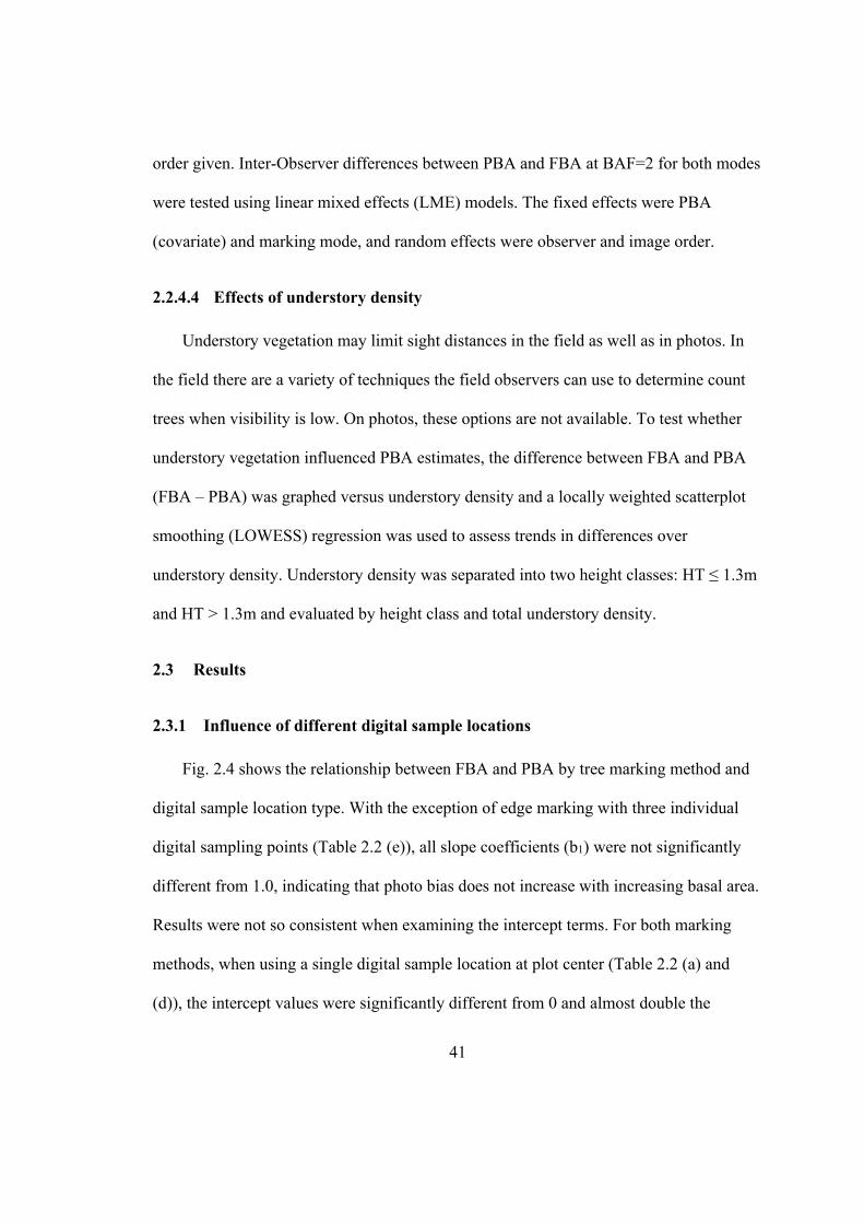
41

order given. Inter-Observer differences between PBA and FBA at BAF=2 for both modes

were tested using linear mixed effects (LME) models. The fixed effects were PBA

(covariate) and marking mode, and random effects were observer and image order.

2.2.4.4 Effects of understory density

Understory vegetation may limit sight distances in the field as well as in photos. In

the field there are a variety of techniques the field observers can use to determine count

trees when visibility is low. On photos, these options are not available. To test whether

understory vegetation influenced PBA estimates, the difference between FBA and PBA

(FBA – PBA) was graphed versus understory density and a locally weighted scatterplot

smoothing (LOWESS) regression was used to assess trends in differences over

understory density. Understory density was separated into two height classes: HT ≤ 1.3m

and HT > 1.3m and evaluated by height class and total understory density.

2.3 Results

2.3.1 Influence of different digital sample locations

Fig. 2.4 shows the relationship between FBA and PBA by tree marking method and

digital sample location type. With the exception of edge marking with three individual

digital sampling points (Table 2.2 (e)), all slope coefficients (b1) were not significantly

different from 1.0, indicating that photo bias does not increase with increasing basal area.

Results were not so consistent when examining the intercept terms. For both marking

methods, when using a single digital sample location at plot center (Table 2.2 (a) and

(d)), the intercept values were significantly different from 0 and almost double the

42

intercept values (b0) obtained using multiple digital sampling points. For the multiple

digital sampling points, only the intercept term for edge marking was significantly

different from 0 (Table 2.2 (e)). Both intercepts for the average of three digital sampling

points were negative, though not significantly different from 0 (Table 2.2 (c) and (f)).

In terms of goodness of fit, the edge marking techniques generally had higher r2

values and lower root mean square error (rMSE) values, indicating a stronger linear

relationship between FBA and PBA (Table 2.2). All regressions indicate an under-

estimation of FBA, except at the very lowest FBA values, when averaging across

multiple digital sampling points. Under-estimation was consistent with the hypothesis of

visibility bias resulting from occluded (hidden or missing) “in” trees. It was expected that

the visibility bias would increase with increasing FBA; however, that was not generally

observed in this study (Table 2.2 and Fig. 2.4).

2.3.2 Effects of BAF choice

It was hypothesized that increasing BAF would result in fewer hidden trees and less

user error in marking edges and that PBA would become closer to FBA; however, that

was not what was observed in this study. Fig. 2.5 shows the effects of increasing BAFs

on PBA estimation. For the NRF plots, the mean differences between FBA and PBA

decreased slightly, but remained positive (underestimation) across all levels of BAF. For

the NL plots, the deviations decreased, but were essentially 0 across all levels of BAF.

The NRF only had one center digital sample location while NL had three sample

locations (Fig. 2.1.a). The additional digital sample points capture a greater range of the

plot variation and reduces the effects of hidden trees. One issue noted on several of the

43

NRF plots was the presence of a tree very close to plot center. Large trees can block

significant view angles on plots. Increasing BAF does not compensate for these

situations. One the other hand, multiple digital sample locations minimized these effects

by locating the camera at different positions within the plot.

For both NRF and NL sites, variation in the differences between FBA and PBA

increased with increasing BAF (Fig. 2.5). Smaller plots are inherently more variable, and

this was an expected outcome. It was expected that there would be an optimal BAF that

minimized differences without substantial increases in variation. This was not observed

in this study. It should be noted that this inference was only based on edge marking

method because of the ease of changing BAF (edges only have to be marked once and all

BAFs could be determined). Results for target counting were not undertaken because

counts would have to be made independently for each BAF tested requiring a significant

increase in image processing time.

2.3.3 Inter-observer consistency

Comparisons between FBA and PBA across the seven volunteers are shown in Fig.

2.6. Most users consistently underestimated FBA with both marking methods, with edge

marking resulting in greater underestimation than target counting (Fig. 2.6. Column 1).

While differences between users were observed (Fig. 2.6. Columns 2-7), on average, user

estimates were comparable (i.e., LOWESS lines were very close to the 1:1 line). Target

counting was generally more consistent than edge marking among different users and

generally resulted in similar estimates across users (Fig. 2.6).

44

Fig. 2.7 shows the two plots with the least and greatest deviations between users. For

the least plot, though different users did not mark exactly the same points across different

trees, the edge positions, as well as the dark gray targets for “in” trees, were almost the

same across users. The simple forest structure facilitates tree marking and results in lower

variability between users. However, it was a different story for the plot with the greatest

deviations. Neither the “out” trees nor the “in” trees have similar positions. Trees were

very dense and diameters smaller, resulting in many “border” trees – small deviations in

edge marking resulted in changes in “in” and “out” status. This problem was further

compounded by the fact that edges of each tree were difficult to distinguish.

To statistically assess the effects of tree marking methods, different users, and image

order (i.e., familiarity with using software), a linear mixed effects (LME) model was

fitted to the data. The full model was:

FBA PBA Marking User Order e (2.5)

where () indicate random effects. A backwards selection method was used to test

significance of random effects. For the full model, the standard deviations associated with

the random effects were: 2.1879 for User and 0.7292 for Order (residual standard error

was 3.7051). The model was refitted with Order excluded and a log likelihood test

performed. The p-value associated with dropping Order was 0.926, indicating that image

order was not a significant random effect influencing deviations from FBA. Similarly,

User was subsequently dropped, and the p-value was 0.081. So, while more significant

than image order, differences between users were still not significant at α =0.05. The final

reduced model only included the fixed effects PBA (covariate) and Marking (method).

Both factors were significant: PBA (p<0.001) and Marking (p<0.01). The root Mean

45

Square Error was 10.6129 and the F value associated with PBA was 320.87 (p < 0.001)

and for Marking Method was 9.913 (p = 0.002).

2.3.4 Understory density effects

Effects of understory density on PBA estimates for the NRF plots are shown in Fig.

2.8. Based on the LOWESS trend lines, understory density did not pose a large visibility

bias in this study. Except for a single plot with very high understory density (> 30000

trees per ha), the trend lines remained around 15 m2/ha, indicating little impact of

understory density on FBA. The value of 15 is very close to the intercept coefficient

estimated above (Table 2.2) and the results here show that the variation in FBA - PBA

(Fig. 2.8) was not due to understory vegetation.

2.4 Discussion

Our results show that spherical images from a consumer-grade 360° camera can

efficiently and effectively estimate basal area using photo-based angle-count sampling.

While underestimation was consistently observed, the trend did not appear to be related

to the amount of basal area per ha present, understory vegetation, nor inter-user

variability. As a result, underestimation could be easily corrected using some form of

double sampling (Dai, 2018, p. 30; Dick, 2012) with ratio correction.

In this study, two photo processing methods were used: the edge marking method

and the octagon target counting method. The resulting PBA estimates were acceptable for

both methods. The advantage of edge marking was that different BAFs can be assessed

without remarking, but this is generally only useful for big BAF sampling (Bell et al.,

1983; Iles, 2003; Marshall et al., 2004) or for research situations where one is interested

46

in effects of different BAFs (as in this study). All users in this study felt the target

counting was more familiar (more similar to the process they used in the field) and more

repeatable than edge marking. Difficulties recognizing tree edges, especially in dense

forest conditions, along with twice the number of mouse clicks for each tree could

potentially cause higher user errors. The octagon target count method avoided potential

edge marking errors and only required one click; however, repeated marking for different

BAFs would be required.

It was expected that visibility bias would increase with increasing basal area because

of an increasing number of hidden trees. This was not observed in this study. There are

several potential explanations for this result. First, and most likely, the results obtained

here were the compensatory effects of underestimation caused by hidden trees coupled

with overestimation caused by increased user error as field basal area increased. In this

study, the plots with the highest basal areas were generally composed of very dense small

stems, especially on the NL sites. With many small trees in an image it can be difficult to

distinguish multiple overlapping small trees from one larger individual tree. With the

edge marking method, it can be very difficult to clearly see the tree edges as well due to

the resolution and exposure conditions (Fig. 2.7.b). Secondly, the plots with very high

basal areas also had a significant number of dead trees present. While care was exercised

to determining live/dead and avoid marking dead trees, this could have increased counts

on the higher basal area plots. Both factors may have also contributed to the lack of

improvement in PBA estimates with increasing BAF.

Multiple digital sampling locations within plots greatly decreased effects of hidden

trees and any user errors. In several individual images there were nearby tree trunks

47

which occluded large portions of the plot radial view. The potential for hidden trees in

these situations was quite large. The multiple digital sample locations minimize this issue

by providing multiple plot viewpoints as well as capturing more of the local spatial

variability. Hidden trees cannot be observed using any remote sensing technique and is a

tough problem to deal with (Ducey and Kershaw, 2011; Ducey and Astrup, 2013; Zasada

et al., 2013). When carrying out field measured angle count sampling, it is possible for

the observer to lean left and right or even slightly change location to identify hidden

trees. Distances from plot center and diameters of hidden trees also can be measured to

determine if hidden trees are count trees or not. This is not possible with photographic or

other remote sensing methods (Fastie, 2010). Building a model to correct for hidden tree

effects can be very complex and should take into account stand density, distance from

tree to sensor, the thickness of each tree trunk, and so on (Zasada et al., 2013). Such

model-based approaches are inherently more variable and require substantial field data to

calibrate (Ducey and Astrup, 2013). A simpler method is to use double sampling with

ratio correction (Dick, 2012; Dai, 2018) or some form of distance sampling correction

(Kershaw, 2010). We have shown another alternative, which is to simply add additional

digital sampling locations within a plot, which is often the solution employed with

terrestrial LiDAR scanning (Seidel et al., 2012; Wallace et al., 2017). Limiting plot size

(or in this case increasing BAF) is another way to decrease effects of hidden trees (Dick

et al., 2010; Zasada et al., 2013); however, this did not seem to be effective in this study.

While multiple digital sample locations improve PBA estimation, it greatly increases

field acquisition time. Given that angle count sampling is already an efficient method to

implement in the field, multiple images would most likely require more field effort.

48

Double sampling with ratio correction is most likely to be the most efficient method for

dealing with hidden trees (Dick, 2012; Dai, 2018).

It is very important to determine an appropriate BAF for angle-count sampling

(Bitterlich, 1984; Iles, 2003; Yang et al., 2017). Choice of BAF greatly influences

variability, which in turn, influences sample size requirements, numbers of trees counted

per plot, and ultimately inventory costs (Iles, 2012; Yang et al., 2017). We found that

BAF could be increased to about 5 without substantially increasing variability. Yang et

al. (2017) obtained similar results for the entire NRF. The increased BAF had the added

effect of slightly reducing visibility bias, thus a trade-off between visibility bias and plot

variation needs to be consider when implementing photo-based angle count sampling.

In this study understory vegetation did not seem to influence visibility bias. Concerns

about effects of understory vegetation has been mentioned by many photo-based forest

inventory studies (Stewart, 2004; Dick et al., 2010; Fastie, 2010; Perng et al., 2018), but

none of these studies verified this effect experimentally. We found that different

understory tree densities had no significant impact on the differences between FBA and

PBA. This was contrary to our expectations. A possible explanation for this phenomenon

is that most of the understory vegetation in the study plots were shorter than 1.3m in

height. Additional advantages in our study include very flat terrain and the ability to view

up the stem and visualize stem size when taller understory vegetation blocked the view.

Variability between different users is a very important consideration when choosing

measurement methods. While a few photo forest mensuration studies have shown that

they can achieve small differences between field measured data and photo measured data

(Clark et al., 2000; Fastie, 2010; Rodríguez-García et al., 2014), none, to our knowledge,

49

have systematically tested the repeatability and reproducibility among different users.

Our repeatability test given by seven volunteers showed: 1) Random effects of image

processing order (familiarity of software) and different users did not have significant

impacts on photo estimation; 2) the denser the plot, the more differences between users

due to manual identification and selection by mouse clicking; and 3) using octagon target

counts did not require identifying tree edges and resulted in lower underestimation than

edge marking.

Many studies have focused on individual tree measurements, then summarizing these

measures into stand level attributes. Some studies use scale tags placed on each tree or

measured field distances and slopes (Dick et al. 2010, Lu et al. 2019). These methods

require measuring or tagging individual trees which is time-consuming and costly and/or

require multiple images for each tree of interest (Stewart et al. 2004, Perng et al. 2018).

These techniques have limited benefit for improving inventory efficiency. In addition,

errors resulting from stitching several digital photos together cannot be avoided (Fastie

2010, Dick et al. 2010, Perng et al. 2018, Lu et al. 2019). Structure from Motion (SfM) is

an “automatic” merging technology which enables 3D reconstruction from photo series

without actual measurements (Snavely et al. 2008). Several studies have used this

technique to reconstruct individual tree stems (Miller et al. 2015, Surový et al. 2016, Mokroš

et al. 2018), or to develop stand level point clouds (Liang et al. 2014, 2015, Forsman et al.

2016, Liu et al. 2018). However, this automatic technology requires obtaining a large

number of photos (Berveglieri et al. 2017a, Liu et al. 2018) and high performance

computers and complex algorithms to conduct analysis (Belton et al. 2013, Liang et al.

2015, Mulverhill et al. 2019). In addition, the points clouds require subsequent

50

measurement to produce the tree and stand attributes. We simply extract the stand-level

basal area directly from the photos.

The method we proposed here has several advantages. First, using a consumer-grade

spherical camera is a very cost-effective (around $400 CDN) and time-effective (less than

1 minute per photo) method. The image is automatically merged in the camera

eliminating the often time-consuming task of acquiring and stitching multiple photos

from different view radii (Dick et al., 2010; Fastie, 2010) or placing reference scale

objects in the field (Dean, 2003; Varjo et al., 2006; Perng et al., 2018). Keeping

permanent digital records for forest plots provides the opportunity for making new

retrospective measurements, this aspect is likely to become more advantageous as novel

technology develops in future (Iles, 1994). Finally, quantification of differences among

users is difficult to assess and correct with most field measurement techniques. The

software developed here keeps a record of individual markings (Fig. 2.7) that could be

used as a comparison reference for correcting photo-based samples.

This study also had some limitations. The camera elevation was not exactly at the

definition of breast height (1.3 m). When selecting tree trunks for marking and estimating

basal area at breast height, we used the equatorial plane of the spherical camera rather

than calculating 1.3m height on tree trunks based on stereoscopic principles (Rodríguez-

García et al., 2014; Sánchez-González et al., 2016; Perng et al., 2018). The spherical

image is merged by two hemispherical lenses, the joint region can sometimes be fuzzy or

blurred which makes tree trunk identification more difficult. Variable sunlight conditions

can result in inconsistent exposure levels across the spherical image. Underexposure

makes trunks in the far distance dark and hard to distinguish while overexposure flashes

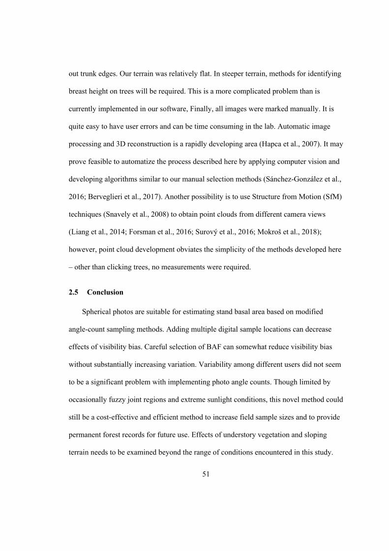
51

out trunk edges. Our terrain was relatively flat. In steeper terrain, methods for identifying

breast height on trees will be required. This is a more complicated problem than is

currently implemented in our software, Finally, all images were marked manually. It is

quite easy to have user errors and can be time consuming in the lab. Automatic image

processing and 3D reconstruction is a rapidly developing area (Hapca et al., 2007). It may

prove feasible to automatize the process described here by applying computer vision and

developing algorithms similar to our manual selection methods (Sánchez-González et al.,

2016; Berveglieri et al., 2017). Another possibility is to use Structure from Motion (SfM)

techniques (Snavely et al., 2008) to obtain point clouds from different camera views

(Liang et al., 2014; Forsman et al., 2016; Surový et al., 2016; Mokroš et al., 2018);

however, point cloud development obviates the simplicity of the methods developed here

– other than clicking trees, no measurements were required.

2.5 Conclusion

Spherical photos are suitable for estimating stand basal area based on modified

angle-count sampling methods. Adding multiple digital sample locations can decrease

effects of visibility bias. Careful selection of BAF can somewhat reduce visibility bias

without substantially increasing variation. Variability among different users did not seem

to be a significant problem with implementing photo angle counts. Though limited by

occasionally fuzzy joint regions and extreme sunlight conditions, this novel method could

still be a cost-effective and efficient method to increase field sample sizes and to provide

permanent forest records for future use. Effects of understory vegetation and sloping

terrain needs to be examined beyond the range of conditions encountered in this study.

52

Future research should focus on other forest attribute extraction such as height and

diameter and automatic image processing.

2.6 Acknowledgements

Funding for this project was provided in part by the National Science and

Engineering Research Council of Canada, Discovery Grants program, the Province of

Newfoundland and Labrador Centre for Forest Science and Innovation Contribution

Agreement, and the New Brunswick Innovation Foundation Research Assistants

Initiative and Graduate Scholarships programs. The authors also thank the lab mates,

collaborators, and summer field crew who helped make this project possible: Emily

Loretta Nicholson, UNB; Dr. Mike Lavigne, Gretta Goodine, and Rodney Foster,

Atlantic Forestry Research Centre, Natural Resources Canada; We also thank Yang Zhan,

Wushuang Li, Shun-Ying Chen, and Yunjia Dai for their volunteer work for software

testing and inter-observer error analysis.

2.7 References

Baskerville, G. 1986. Understanding forest management. Forestry Chronicle 62:339–347.

Bell, J. F., K. Iles, and D. Marshall. 1983. Balancing the ratio of tree count-only sample

points and VBAR measurements in variable plot sampling.Bell J.F. and

Atterbury, T. (eds.). Proceedings: Renewable Resource Inventories for

Monitoring Changes and Trends. College of Forestry, Oregon State University,

Corvallis, OR. pp. 699–702.

Belton, D., S. Moncrieff, and J. Chapman. 2013. Processing tree point clouds using

Gaussian Mixture Models. ISPRS Annals of Photogrammetry, Remote Sensing

53

and Spatial Information Sciences. Copernicus GmbH, Antalya, Turkey. pp. 43–

48.

Berveglieri, A., A. Tommaselli, X. Liang, and E. Honkavaara. 2017a. Photogrammetric

measurement of tree stems from vertical fisheye images. Scandinavian Journal of

Forest Research 32:737–747.

Berveglieri, A., A. M. G. Tommaselli, X. Liang, and E. Honkavaara. 2017b. Vertical

Optical Scanning with Panoramic Vision for Tree Trunk Reconstruction. Sensors

17(2791).

Bettinger, P., K. Boston, J. Siry, and D. Grebner. 2017. Forest Management and

Planning. 2nd edn. Academic Press, San Diego, CA.

Bitterlich, W. 1947. Die winkelzählmessung (Measurement of basal area per hectare by

means of angle measurement.). Allgemeine Forst- und Holzwirtschaftliche

Zeitung 58:94–96.





Christensen, N. L., A. M. Bartuska, J. H. Brown, S. Carpenter, C. D’Antonio, R. Francis,

J. F. Franklin, J. A. MacMahon, R. F. Noss, D. J. Parsons, C. H. Peterson, M. G.

Turner, and R. G. Woodmansee. 1996. The report of the Ecological Society of

America committee on the scientific basis for ecosystem management. Ecological

Applications 6:665–691.

54

Clark, N. A., R. H. Wynne, D. L. Schmoldt, and M. Winn. 2000. An assessment of the



Clutter, J. L., J. C. Fortson, L. V. Pienaar, G. H. Brister, and R. L. Bailey. 1983. Timber

management. A quantitative approach. First. John Wiley & Sons, New York.

Dai, X. 2018. Bias correction in panoramic photo-based angle count sampling. Unpub.

BScF Honors, University of New Brunswick, Fredericton, NB, Canada.

Dean, C. 2003. Calculation of wood volume and stem taper using terrestrial single-image

close-range photogrammetry and contemporary software tools. Silva Fennica

37:359–380.

DeCourt, N. 1956. Utilisation de la photographie pour mesurer les surfaces terrières (The

use of photography for measuring basal area). Revue Forestière Française 8:505–

507.

Dick, A. R. 2012. Forest inventory using a camera: Concept, field implementation and

instrument development. Unpublished MScF Thesis, University of New

Brunswick, Fredericton, NB, Canada.



Ducey, M. J., and R. Astrup. 2013. Adjusting for nondetection in forest inventories

derived from terrestrial laser scanning. Canadian Journal of Remote Sensing

39:410–425.

Ducey, M. J., and J. A. Kershaw. 2011. Vertical Point Sampling with a Camera. Northern

Journal of Applied Forestry 28:61–65.

55

Fastie, C. L. 2010. Estimating stand basal area from forest panoramas. Page 8

Proceedings of the Fine International Conference on Gigapixel Imaging for

Science. Carnegie Mellon University, Pittsburg, PA.

Forsman, M., N. Börlin, and J. Holmgren. 2016. Estimation of Tree Stem Attributes

Using Terrestrial Photogrammetry with a Camera Rig. Forests 7(61).

Gillis, A. M. 1990. The New Forestry. BioScience 40:558–562.

Grosenbaugh, L. R. 1952. Plotless timber estimates--New, fast, easy. Journal of Forestry

50:32–37.

Grosenbaugh, L. R. 1958. Point-sampling and line-sampling: Probability theory,

geometric implications, synthesis. Page 34. Occasional Paper, USDA Forest

Service, Southern Forest Experiment Station.

Grosenbaugh, L. R. 1963. Optical dendrometers for out-of-reach diameters: A conspectus

and some new theory. Forest Science Monographs 4(48).

Guido, van R. 2018. Python (programming language). Python Software Foundation, US.

Url: https://docs.python.org/3.6/reference/index.html. Last Accessed 12-11-2018.

Hapca, A. I., F. Mothe, and J.-M. Leban. 2007. A digital photographic method for 3D

reconstruction of standing tree shape. Annals of Forest Science 64:631–637.

Husch, B. 1980. How to determine what you can afford to spend on inventories. IUFRO

Workshop on Arid Land Resource Inventories. USDA, Forest Service,

Washington Office, General Technical Report WO-28, La Paz, Mexico. pp. 98–

102

Iles, K. 1994. Directions in Forest Inventory. Journal of Forestry 92:12–15.

56


Nanaimo, BC.

Iles, K. 2012. Some Current Subsampling Techniques in Forestry. Mathematical &

Computational Forestry & Natural Resource Sciences 4(2).

Jenkins, J. C., D. C. Chojnacky, L. S. Heath, and R. A. Birdsey. 2003. National scale

biomass estimators for United States tree species. Forest Science 49:12–35.

Kershaw, J. A., Jr. 2010. Correcting for visibility bias in photo point samples.

Stockbridge, MA.





Liang, X., A. Jaakkola, Y. Wang, J. Hyyppä, E. Honkavaara, J. Liu, and H. Kaartinen.

2014. The Use of a Hand-Held Camera for Individual Tree 3D Mapping in Forest

Sample Plots. Remote Sensing 6:6587–6603.

Liang, X., Y. Wang, A. Jaakkola, A. Kukko, H. Kaartinen, J. Hyyppä, E. Honkavaara,

and J. Liu. 2015. Forest Data Collection Using Terrestrial Image-Based Point

Clouds From a Handheld Camera Compared to Terrestrial and Personal Laser

Scanning. IEEE Transactions on Geoscience and Remote Sensing 53:5117–5132.

Liu, J., Z. Feng, L. Yang, A. Mannan, T. U. Khan, Z. Zhao, and Z. Cheng. 2018.

Extraction of Sample Plot Parameters from 3D Point Cloud Reconstruction Based

on Combined RTK and CCD Continuous Photography. Remote Sensing

10(1299).

57

Lootens, J. R., D. R. Larsen, and S. R. . Shifley. 2007. Height-diameter equations for 12

upland species in the Missouri Ozark Highlands. Northern Journal of Applied

Forestry 24:1149–1152.

Lu, M.-K., T. Y. Lam, B.-H. Perng, and H.-T. Lin. 2019. Close-range photogrammetry

with spherical panoramas for mapping spatial location and measuring diameters

of trees under forest canopies. Canadian Journal of Forest Research 49:865–874.



34:840–845.

Miller, J., J. Morgenroth, and C. Gomez. 2015. 3D modelling of individual trees using a

handheld camera: Accuracy of height, diameter and volume estimates. Urban

Forestry & Urban Greening 14:932–940.




Mulverhill, C., N. C. Coops, P. Tompalski, C. W. Bater, and A. R. Dick. 2019. The utility

of terrestrial photogrammetry for assessment of tree volume and taper in boreal

mixedwood forests. Annals of Forest Science 76(83).

Opie, J. E. 1968. Predictability of Individual Tree Growth Using Various Definitions of

Competing Basal Area. Forest Science 14:314–323.




58




Ricoh Imaging Company, LTD. 2016. Rioch Theta S 360 video camera.

http://www.ricoh-imaging.co.jp/english/products/theta\_s/. Last Accessed 26-08-

2016.

Rodríguez-García, C., F. Montes, F. Ruiz, I. Cañellas, and P. Pita. 2014. Stem mapping

and estimating standing volume from stereoscopic hemispherical images.

European Journal of Forest Research 133:895–904.

Rowe, J. S. 1972. Forest Regions of Canada. Publication, Fisheries and Environment

Canada, Canadian Forest Service, Headquarters, Ottawa. 172 p.

Sánchez-González, M., M. Cabrera, P. J. Herrera, R. Vallejo, I. Cañellas, and F. Montes.

2016. Basal Area and Diameter Distribution Estimation Using Stereoscopic

Hemispherical Images. Photogrammetric Engineering & Remote Sensing 82:605–

616.

Seidel, D., S. Fleck, and C. Leuschner. 2012. Analyzing forest canopies with ground-

based laser scanning: A comparison with hemispherical photography. Agricultural

and Forest Meteorology 154–155:1–8.

Slik, J. W. F., S.-I. Aiba, F. Q. Brearley, C. H. Cannon, O. Forshed, K. Kitayama, H.

Nagamasu, R. Nilus, J. Payne, G. Paoli, A. D. Poulsen, N. Raes, D. Sheil, K.

Sidiyasa, E. Suzuki, and J. L. C. H. van Valkenburg. 2010. Environmental

correlates of tree biomass, basal area, wood specific gravity and stem density

59

gradients in Borneo’s tropical forests. Global Ecology and Biogeography 19:50–

60.

Snavely, N., S. M. Seitz, and R. Szeliski. 2008. Modeling the World from Internet Photo

Collections. International Journal of Computer Vision 80:189–210.

Stewart, B. 2004, August. Using a camera as an angle gauge in angle-count sampling.

MF Thesis, The University of Georgia.

Stewart, B., C. J. Cieszewski, and M. Zasada. 2004. Use of a camera as an angle-gauge in

angle-count sampling. Second International Conference on Forest Measurements

and Quantitative Methods and Management. Warnell School of Forestry and

Natural Resources, University of Georgia, Athens, GA. pp. 375–380

Surový, P., A. Yoshimoto, and D. Panagiotidis. 2016. Accuracy of Reconstruction of the

Tree Stem Surface Using Terrestrial Close-Range Photogrammetry. Remote

Sensing 8:123.

Varjo, J., H. Henttonen, J. Lappi, J. Heikkonen, and J. Juujärvi. 2006. Digital horizontal

tree measurements for forest inventory. Working papers of the Finnish Forest

Research Institute 40(23).

Wallace, L., S. Hillman, K. Reinke, and B. Hally. 2017. Non-destructive estimation of

above-ground surface and near-surface biomass using 3D terrestrial remote

sensing techniques. Methods in Ecology and Evolution 8:1607–1616.

Weiskittel, A. R., D. W. Hann, J. A. Kershaw Jr., and J. K. Vanclay. 2011. Forest Growth

and Yield Modeling. 2nd edition. Wiley/Blackwell, New York.



60



Zar, J. H. 2009. Biostatistical analysis. 5th edition. Pearson, New York.

Zasada, M., K. Stereńczak, W. M. Dudek, and A. Rybski. 2013. Horizon visibility and

accuracy of stocking determination on circular sample plots using automated

remote measurement techniques. Forest Ecology and Management 302:171–177.

61

Table 2.1: Average stand-level estimates (standard errors in parentheses) by trial and treatment for the 3 early spacing trials located with western

Newfoundland.

Trial Year Treatment Stand-Level Averages (Standard Errors) Trees (num/ha) Basal Area (m2/ha) DBH (cm) Total Height (m) Cormack 2013 Control (no spacing) 9974 (1807) 62.39 (6.26) 8.97 (0.42) 9.21 (0.92) 1.2m spacing 6239 (740) 49.94 (9.49) 10.14 (1.60) 8.86 (1.63) 1.8m spacing 2978 (433) 34.41 (10.88) 12.07 (1.64) 8.73 (1.61) 2.4m spacing 1432 (168) 32.38 (3.81) 16.98 (0.59) 10.62 (0.54) 3.0m spacing 965 (62) 21.54 (0.92) 16.86 (0.18) 9.62 (0.23) Pasadena 2013 Control (no spacing) 6112 (2049) 61.04 (9.36) 11.52 (1.27) 9.83 (0.82) 1.2m spacing 3616 (863) 67.22 (5.07) 15.59 (1.95) 11.37 (1.38) 1.8m spacing 2611 (309) 53.59 (7.29) 16.16 (0.16) 10.81 (0.43) 2.4m spacing 1793 (545) 46.18 (10.12) 18.26 (0.86) 11.35 (0.29) 3.0m spacing 1111 (61) 36.88 (3.04) 20.55 (0.58) 11.60 (0.33) Roddickton 2017 Control (no spacing) 12775 (2101) 73.19 (8.06) 8.59 (0.88) 7.07 (0.62) 1.2m spacing 4987 (1066) 54.62 (4.61) 11.94 (1.47) 8.28 (1.28) 1.8m spacing 2927 (247) 40.58 (2.86) 13.30 (0.50) 7.94 (0.25) 2.4m spacing 2119 (253) 40.40 (9.13) 15.50 (0.85) 8.74 (0.67) 3.0m spacing 1253 (87) 31.25 (2.21) 17.83 (0.41) 9.12 (0.35)

62

Table 2.2: Simple linear regression results for field basal area versus photo basal area by digital sample point type. The linear model is FBA=b0 + b1*PBA,

if PBA is the same as FBA, then b0=0 and b1=1

Photo marking mode Digital sample points type Parameters Estimate Standard Error p-value r2 rMSE Target Counting (a) One center estimate b0 19.74 3.85 <0.001 0.41 9.27 b1 0.84 0.11 0.150 (b) Three individual estimates b0 4.44 3.08 0.152 0.61 9.66 b1 0.99 0.06 0.868 (c) Mean of three estimates b0 -5.22 4.79 0.282 0.75 7.77 b1 1.21 0.11 0.063 Edge Marking (d) One center estimate b0 15.69 4.09 <0.001 0.44 9.00 b1 0.83 0.10 0.093 (e) Three individual estimates b0 7.34 2.91 0.013 0.60 9.72 b1 0.88 0.06 0.048 (f) Mean of three estimates b0 -4.04 4.32 0.355 0.78 7.30 b1 1.13 0.09 0.158

63

Fig. 2.1: Digital data collection methods: (a) Digital sample location design for Newfoundland (NL) and Noonan Research Forest (NRF) (Three locations

were established at the midpoint of plot radius along azimuths of 120°, 240°, and 360° in each NL plot, while only one location was set in the center for

each NRF plot); (b) tripod and camera set up for spherical image acquisition.

64

Fig. 2.2: Sample geometry. For angle count sampling: (a) overhead view showing “in”, “border” and “out” tree (gray circles represent tree trunks); (b) the

relationship between horizontal angle (θ), tree diameter (D) and plot (inclusion zone) radius (R). The BAF determines the fixed horizontal angle θ which

was used as the threshold to determine tree status on the spherical images.

65

Fig. 2.3: Two image processing methods: (a) Edge marking method – users click on the edges of each tree. A reference bar (the length is based on BAF=1)

is used to guide users so that every tree does not have to be marked; the line color indicates tree status based on desired BAF: black = “in”, gray = “out”);

(b) Target count method - a transparent reference octagon, scaled to the desired BAF is provided to mark “in” trees - “out” trees are those trees smaller than

the octagon target and are not marked.

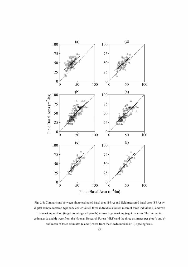
66

Fig. 2.4: Comparisons between photo estimated basal area (PBA) and field measured basal area (FBA) by

digital sample location type (one center versus three individuals versus mean of three individuals) and two

tree marking method (target counting (left panels) versus edge marking (right panels)). The one center

estimates (a and d) were from the Noonan Research Forest (NRF) and the three estimates per plot (b and e)

and mean of three estimates (c and f) were from the Newfoundland (NL) spacing trials.

67

Fig. 2.5: The influence of photo basal area factor (BAF) choice on the basal area difference (field basal area – photo basal area, m2/ha) for Newfoundland

(NL) and Noonan Research Forest (NRF). The black solid line is the mean for each location and the gray dashed line indicates perfect fit

68

Fig. 2.6: Comparisons between field basal area and photo basal area by two marking methods (edge

marking versus target counting) among seven different users. The locally weighted scatterplot smoothing

(LOWESS) regression lines show the trends between field measure and photo.

69

Fig. 2.7: Two plots with the smallest (a) and largest (b) variance among seven users by two tree marking

methods (edge marking versus target counting). PBA means photo-based basal area and FBA means field-

based basal area. The FBA of (a) is 30 m2/ha, and FBA of (b) is 55.2 m2/ha. The small dots are the tree

edges that users marked. The black small dot with connected lines means this tree is counted as an “in”

tree, while the light gray small dots means it is an “out” tree in edge marking mode. The dark gray octagon

is the “in” tree marked in target counting mode.

70

Fig. 2.8: Effects of understory density on the basal area difference (field basal area – photo basal area, m2/ha) in the NRF plots by two marking methods

(target counting (left panels) versus edge marking (right panels)). (a) and (d) are total understory trees, (b) and (e) are understory trees whose height smaller

than 1.3 m, while (c) and (f) are those greater than 1.3 m.

71

Chapter 3: Plant Fraction Calculation from Spherical Images by HSV Color Space

3.1 Introduction

Applications of image analysis in forest inventory can be traced back to the middle

of the 20th century. For example, Reineke (1940) used photos to establish a permanent

plot record, Shelbourne and Namkoong (1966) developed a method for measuring trunk

parameters based on image geometry. Upper canopy information and light conditions

were first recorded using a hemispherical camera with a fisheye lens called the Robin Hill

camera (Evans and Coombe 1959) which produced a single image by converting a full

hemisphere to a circular plane with a polar projection (Coombe and Evans 1960, Rich et

al. 1999). Forestry and ecological researchers developed methods to maximize the

benefits of hemispherical images and improved and standardized the acquisition,

analysis, and interpretation of images using hemispherical photos (Fournier and Hall

2017 p. 2).

Initially, analyses were based on manual processing of film images, and the

information extracted from hemispherical photos was primarily used to calculate sunlight

penetration and solar radiation through canopy openings (Fournier and Hall 2017 p. 3).

Manual processing methods were slow and often subjective. With the advent of the

digital camera and personal computer, the technology to process hemispherical

photographs developed into a more automated, precise analysis based on the geometric

distributions of plant structural elements (Rich 1990, Chen et al. 1991). Analyzing

canopy gap information to derive canopy structure became a focus of research in forestry

and ecology (van Gardingen et al. 1999, Leblanc et al. 2005, Cescatti 2007). The

72

improvement in image resolution, dynamic range of sensors, and richness of image

processing software greatly improved the procedures for hemispherical image acquisition

and analysis compared to film-based photography (Chianucci and Cutini 2012, Fournier

and Hall 2017 p. 117). Several studies have emphasized the effects of this revolution,

especially in terms of image resolution and digitalization (Englund et al. 2000, Inoue et

al. 2004).

Currently, image processing software can be separated into two types: commercial

software and open source (free or low cost) software. Open source software includes:

CAN-EYE (Baret and Weiss 2004), CIMES (Gonsamo et al. 2011), and GLA (Frazer et

al. 1999). Commercial software includes: HemiView (Rich et al. 1999), and

WinSCANOPY (Regent Instruments Inc. 2018). Several studies have compared different

software (Bréda 2003, Jarčuška et al. 2010, Promis et al. 2011, Fournier and Hall 2017

chap. 7). Based on these studies, it is hard to draw conclusions about which is best; it

depends on user preference, type of camera, and costs (free or commercial). Batch

processing options are often very important (Fournier and Hall 2017 chap. 5). While

well-integrated software is convenient to use, the flexibility to adjust to personal

requirements and incorporation of new processing algorithms is often limited. As a result,

several researchers chose to write their own programs to apply their novel ideas in image

processing, including: DHPT (Loffredo et al. 2016), HSP (Lang et al. 2013), and the

ImageJ Hemispherical_2.0 extension (Rasband 1997, Beckschäfer 2015).

As Chianucci and Cutini (2012) and Fournier and Hall (2017) summarized, the

processing of forest hemispherical images has four main steps: 1) Image acquisition and

73

quality control; 2) Image enhancement (optional); 3) Sky and canopy pixel classification

(binarization); and 4) Extraction of attributes from classified binary images.

The first step is to obtain suitable images. Hemispherical images are normally taken

in summer when canopies are fully developed. The ideal sunlight conditions are close to

sunrise or sunset or when the sky is uniformly overcast (Leblanc et al. 2005). Uneven sky

radiance and clouds complicate image analysis (Fournier and Hall 2017 p. 119). Zhang et

al. (2005) pointed out that the exposure settings of cameras have great impacts on gaps

and its fractional determination. Default auto-exposures often do not yield accurate and

consistent gap fraction estimates (Chen et al. 1991, MacFarlane et al. 2000, Zhang et al.

2005). The best exposures for simple classification are set manually to ensure the sky is

well diffused and appears almost white and the contrast between sky and plant is

maximized (Chen et al. 1991). Generally, the most suitable manual setting is to

overexpose images by 1 – 3 f-stops of shutter speed relative to the reference exposure

measured in clear sky (Zhang et al. 2005).

The second (optional) step is image enhancement. A common enhancing filter is

sharpening based on edge enhancement provided by almost all software packages. Edge

enhancement is used to increase the contrast between small gaps and dense canopies. It is

most useful for low resolution images containing a large proportion of mixed pixels,

which means the pixel includes several different classes (Fournier and Hall 2017 p. 121).

Gamma correction is another option. Although digital cameras respond linearly to light

(Zhang et al. 2005), most camera software automatically applies a gamma logarithmic

transformation to simulate the non-linear behavior of the human eye (Cescatti 2007).

Commonly the gamma value of a camera ranges between 2.0 to 2.5 and darkens the

74

midtones of an image. This often worsens the estimates of gaps within canopies (Cescatti

2007). MacFarlane et al. (2007a, 2007b) pointed out that restoring gamma values to 1.0

helps solve the large errors in those images. For cameras that record RAW image

formats, the gamma function correction is unnecessary and can be easily transferred to

binary images by linear transformation (Lang et al. 2010).

The third step is classification. Because of the importance of thresholding

segmentation and pixel classification, this step has been thoroughly investigated over the

past few decades, as Wagner and Hagemeier (2006) reviewed. Even though common

digital images have three color channels (Red, Green, and Blue, RGB), most studies only

use gray-scale values (0-255) from the blue channel for classification (Leblanc et al.

2005, Zhang et al. 2005, MacFarlane 2011). The blue portion of light is absorbed by plant

pigments and darkens the foliage in hemispherical photos (Leblanc et al. 2005,

Jonckheere et al. 2005). Using a single channel has the additional benefit of avoiding

aberrations caused by lens imperfections (Frazer et al. 2001, Leblanc et al. 2002, Fournier

and Hall 2017 chap. 5). Six binarization algorithms based on blue channel histograms

were reviewed by Glatthorn and Beckschäfer (2014); however, all algorithms were

sensitive to overexposure. Exposures need to be strictly controlled when taking images.

Beckschäfer et al. (2013) suggested using the camera screen to check histograms in the

field to determine whether exposures were suitable or not.

Even though images are well exposed and taken in deeply overcast conditions,

luminance heterogeneity always exists (Wagner 1998, 2001, Schwalbe et al. 2006,

Fournier and Hall 2017 p. 125). To minimize its effects, instead of using a global

threshold in which a single threshold is applied to an entire image, different regional

75

thresholds are applied to parts of images according to the zenith and horizon angles

(Wagner 1998, Leblanc et al. 2005, Fournier and Hall 2017 p. 127). Appling different

thresholds for different canopy densities has been explored as well (MacFarlane 2011).

However, these optimization algorithms narrowed their attention to only blue channel

information, rather than considering full color information and textural differences

between sky and canopy.

With the development of computer vision algorithms, some novel algorithms such as

edge detection (Nobis and Hunziker 2005, Glatthorn and Beckschäfer 2014) and

integrated RGB channels with different weights based on brightness obtained by hue

values (Loffredo et al. 2016) or external light sensors (Zhao and He 2016) have displayed

better tolerance to overexposure. Converting RGB color space to HSV (hue, saturation,

and value) color space (Riaz et al. 2008) is another option, For example, Chumuang et al.

(2016) used hue ranges from 110 to 130 (255 maximum) to classify green leaves and

white background while Yang et al. (2015) used an HSV decision tree to classify green

vegetation from soil background. However, both HSV methods were applied to a

common digital camera image. Based on our current literature search, this classification

method has not been applied to hemispherical images.

The fourth step is extracting canopy attributes from classified binary images. This is

a standard procedure for many hemispherical image analysis software packages.

Attributes, such as canopy closure, gap fraction, canopy openness, and so on, are well

defined by Gonsamo et al. (2013). However, for fisheye cameras, two things need

consideration: projection distortion and lens vignetting (Fournier and Hall 2017 chap. 5).

Projection distortion occurs when the fisheye lens does not conform, or strictly conform,

76

to perfect polar or equidistant projection due to manufacture defects (Herbert 1987). In

these cases, additional calibration is required (Frazer et al. 2001). Lens vignetting is due

to the structure of the fisheye camera, the wide aperture always results in gradual light

fall-off near the outer image edges. Although this can be improved by applying correction

algorithms, the light conditions are difficult to correct to true values (Wagner 1998, 2001,

Schwalbe et al. 2006).

The new 360-degree spherical cameras offer an inexpensive option for obtaining full

spherical stand information with one exposure. The friendly price and compact size make

it an easy-to-use tool in the forest and may be an acceptable alternative to traditional

fisheye cameras. The purpose of this chapter is to explore whether spherical cameras can

be used to extract canopy information and whether a novel HSV threshold can produce

similar, or even enhanced, classification results compared to traditional blue channel-

based classification algorithms. Specific objectives include: 1) propose a global HSV

classification threshold to classify images into three classes: sky, foliage, and wood; 2)

compare the new HSV threshold with a blue channel-based minimum threshold as

implemented by ImageJ Hemispherical_2.0 extension (Beckschäfer 2015); 3) compare

hemispherical and cylindrical projections of spherical images using the HSV threshold

technique and analyze the consistency between projections.

3.2 Methods and Materials

3.2.1 Study sites

There were two different sites used in this study. The first site was three early

spacing trails located in western Newfoundland (NL). These sites (Cormack, Pasadena,

77

and Roddickton, Fig. 3.1) were dominated by balsam fir (Abies balsamea) with minor

components of black spruce (Picea mariana) and other boreal species. The trials were

established in the early 1980’s. At each trial, there were three replicates of five spacing

treatments: Control (no spacing), 1.2m, 1.8m, 2.4m, and 3.0m average spacing. Because

of the early spacing treatments, the NL plots are even-aged, single stratum stands with

relatively uniform stand structure.

The second site was the Femelschlag Research Study located on the Noonan

Research Forest (NRF) in central New Brunswick, Canada (Fig. 3.1). The NRF plots

were composed of a variety of stand types from pure coniferous stands to mixed

hardwood-softwood stands. Because of the variety of stand types, the NRF plots were

much more structurally diverse. A permanent 100m by 100m inventory sample grid was

overlaid on the NRF in 1999. The 83 grid intersections within the Noonan Femelschlag

Research Study were used in this study. Table 3.1 summarizes the species composition

across the two study areas.

3.2.2 Digital data acquisition

A Ricoh Theta S (Ricoh Imaging Company, LTD. 2016) spherical camera was used

to capture spherical images. Four single spherical images were captured at four different

heights (1.6m, 2.6m, 3.6m, 4.6m) at each digital sampling point (Fig. 3.2.a) using a

height pole (Fig. 3.2.b). On the NL sites, three digital sample points per replicate plot

were used. Digital sample points were located at half the plot radius at azimuths of 360°,

120°, and 240°. Plot radii varied by spacing treatment: Control (5.2m);1.2m (7.2m); 1.8m

78

(10.4m); 2.4m (15.0m); 3.0m (18.0m). On the NRF plots a single digital sampling point

was located at plot center (Fig. 3.2.a).

Although the spherical camera records a 3D image, the image is stored as a 2D

digital image based on cylindrical equidistant projection using on-board camera software.

The resolution of the projected 2D cylindrical images was 5367 pixels in width and 2688

pixels in height.

3.2.3 Image processing methods

Even though hemispherical cameras take full 360°/180° images, because of the

projection distortion (Blennow 1995), resolution considerations (Leblanc et al. 2005),

light degradation (Wilson 1963, Wagner 1998, Schwalbe et al. 2006), and biological

considerations (lower parts of stems dominate more than canopy foliage) only the higher

zenith angles of the hemispherical images were used. Based on these previous studies,

Plant fraction (PF), in this study, was defined as the fraction of the image occupied by

plant pixels within a 57.5° zenith angle after distortion calibration (PF57.5) rather than

using the full 90° hemispherical images. (Weiss et al. 2004, Jonckheere et al. 2005).

Two different approaches to calculate PF were developed in this study, the general

workflow is shown in Fig. 3.4. One approach converted cylindrical images to

hemispherical images first, then applied common fisheye processing methods

(hemispherical approach), the other approach directly applied a weight function to

classified cylindrical images (cylindrical approach). The hemispherical approach was

good for comparing the new method with traditional image processing methods, while

the cylindrical approach was more efficient for image processing.

79

3.2.3.1 Hemispherical Approach

There were three steps to estimate plant fraction from spherical images in this

approach: 1) conversion from the stored cylindrical image to a hemispherical image; 2)

distortion correction; and 3) threshold classification.

1) Image Transformation

The 3D spherical images were stored as 2D cylindrical images. To transform the

cylindrical image to a hemispherical image, the spherical coordinates were required as an

intermediate transformation. For a given point, C 𝑥 ,𝑦 , in the x-y pixel coordinate

system of the cylindrical image (Fig. 3.4.a), the related zenith angle (𝜑 ) and azimuth

angle (𝜆 ) within the 3D spherical coordinate system (S, Fig. 3.4.b) was calculated using

(Aghayari et al. 2017):

𝑆 𝜆 ,𝜑 ⇒𝜆 𝑋 𝑥

2𝜋𝑋

𝜑 𝑦𝑌2

0.5𝜋𝑌

(3.1)

where X was the cylindrical image width in pixels (5367 pixels for the images used in

this study) Y was the cylindrical image height in pixels (2688 pixels for the images used

in this study); 𝑥 is the horizontal pixel coordinate; and 𝑦 is the vertical pixel coordinate

(Fig. 3.4.d). The zenith angle (𝜑 ) ranged from -π/2 (-90°) to π/2 (90°) while the azimuth

angle (𝜆 ) ranged from 0 (0°) to 2π (360°).

The points in spherical coordinates (S, Fig. 3.4.b) were then projected to

hemispherical coordinates (H, Fig. 3.4.c) using:

80

𝐻 𝑚 ,𝑛 ⇒𝑚

𝑌2

sin 𝜆 ∙ 𝑟

𝑛𝑌2

cos 𝜆 ∙ 𝑟 (3.2)

where 𝑟 is the radius from fisheye center to the projected point:

𝑟𝑌2∙

0.5𝜋 𝜑 0.5𝜋

(3.3)

Duplicate pixels in the converted hemisphere image (for example, all pixels in the

first line of the original cylindrical image were converted to one center pixel in

hemispherical image), were averaged as the final pixel value in the hemisphere image.

For pixels in converted hemispherical images with no values (holes), the average value of

the eight-neighbor pixels was used.

2) Distortion correction

As shown in Fig. 3.4.c, the projected hemispherical images had distortion (note how

the edges of the ceiling light fixtures curve). To correct the distortion, an equisolid

distortion correction method (Hughes et al. 2010) was applied:

𝑟 ′𝑋

2√2∙ 𝑡𝑎𝑛 2 ∙ 𝑎𝑟𝑐𝑡𝑎𝑛

𝑟

√2𝑋2

(3.4)

the distortion corrected point H′ 𝑚 ,𝑛 in hemispherical coordinates (Fig. 3.4.d) was

then equal to:

𝐻′ 𝑚 ,𝑛 ⇒𝑚

𝑌2

sin 𝜆 ∙ 𝑟

𝑛𝑌2

cos 𝜆 ∙ 𝑟 (3.5)

The procedures for averaging duplicates and filling holes were the same as those in

previous step.

81

3) Threshold classification

In this step, the HSV color space threshold is applied to classify the pixels into three

classes (foliage-green; wood-red; and sky-blue; 3 color image) or two classes (plant-

white; sky-black; binary image). Unlike RGB color space that uses the three primary

colors (red, green, blue) to combine into a new color, the HSV color space uses attributes

of hue, saturation, and brightness (value) to represent colors (Hanbury and Serra 2002).

The main benefit of using HSV color space was that it was easier to use simple

linear boundaries (rectangles) to distinguish different classes such as sky pixels in

different weather conditions and foliage pixels (Fig. 3.3). The thresholds applied in this

study were Clear Sky (S1): (0.5<h<0.68, 0.45<s<1, 0.75<v<1), Diffused Sky (S2):

(0.48<h<0.61, 0.15<s<0.45, 0.85<v<1), Cloudy Sky (S3): (0<h<1, 0<s<0.15, 0.88<v<1),

and Foliage (F): (0.17<h<0.48, 0.15<s<0.45, 0.2<v<1). The remaining space was

assumed to represent woody plant parts.

After pixel classification, hemispherical plant fraction (HPF), was calculated as the

proportion of pixels covered by plants (foliage and wood):

𝐻𝑃𝐹𝑐𝑜𝑢𝑛𝑡 𝑜𝑓 𝑝𝑙𝑎𝑛𝑡 𝑝𝑖𝑥𝑒𝑙𝑠𝑐𝑜𝑢𝑛𝑡 𝑜𝑓 𝑎𝑙𝑙 𝑝𝑖𝑥𝑒𝑙𝑠

(3.6)

Similarly, hemispherical wood fraction (HWF) or hemispherical foliage fraction (HFF)

was obtained by counting wood pixels or foliage pixels and dividing by total pixels.

3.2.3.2 Cylindrical Approach

The hemispherical approach was suitable for producing images to be used in

traditional fisheye analysis software, however, it was possible to estimate PF directly

from the cylindrical images without coordinate conversion. The procedure applied the

82

HSV classification algorithm directly to the cylindrical image and determined PF for each

pixel line (CPFl, cylindrical plant fraction of line l). Total CPF was then obtained by

summing the CPFl multiplied by a weight that represented a functional transformation

from row length to hemispherical annulus.

The classification procedure was the same as for the hemispherical approach

described above, just applied directly to the cylindrical image. The weight of row l was

calculated based on the relative area of the annulus of the circle at row l.

𝑤𝐴 𝑙 𝐴 𝑙 1

𝐴 859∙ (3.7)

where A(l) was the area of the hemispherical circle at row l, and 𝐴 𝑙 π ∙ 𝑟 . In this

equation, 𝑟 was the corrected hemispherical radius at row l 𝑙. .⎯⎯⎯⎯ 𝜑

. .⎯⎯⎯⎯ 𝑟

. .⎯⎯⎯⎯ 𝑟 . 859 is the row number of 57.5° zenith angle in this study ( ∙

.∙

.858.6), so 𝑙 is the circle boundary in hemispherical images and maximum row

in cylindrical images.

The cylindrical plant fraction, CPF, was then calculated:

𝐶𝑃𝐹 𝐶𝑃𝐹 ∙ 𝑤 (3.8)

Similarly, cylindrical wood fraction (CWF) or cylindrical foliage fraction (CFF) can

be obtained using the same process.

The hemispherical approaches and cylindrical approaches are quite different. The

cylindrical approach is quite similar with the most common approaches applied by

several fisheye analysis software: plant fraction is estimated by dividing the image into

83

several zenith annuli and azimuthal sectors (Fournier and Hall 2017 p. 133). The PF in

each sector is calculated and given a corresponding weight determined by a calibration

algorithm. The total PF (within 57.5° zenith angle) is obtained by summing all of the

sector PFs multiplied by their associated calibration weight. However, for the

hemispherical approach, the calibration function is applied first, then the classification

algorithm is used to create binary images. Which means, the hemispherical approach

measures PF at the pixel-level, while the common methods and cylindrical approach

applies calibration weight at the sector (or annulus) level.

3.2.4 Data analysis

We did not have access to a standard fisheye camera, so we are unable to compare

360° photos to standard hemispherical photos. Our analyses will instead focus on two

aspects: 1) Comparison of the HSV classification method proposed here with the

commonly used Blue-channel thresholding method; and 2) Comparison of PF estimated

from cylindrical photos (CPF) to estimates from hemispherical photos (HPF).

3.2.4.1 Comparison of classification methods

We used two analyses to examine differences between the HSV classification

method and the Blue-channel threshold method. For estimation of leaf area index,

photography is generally restricted to a few hours in the morning and late afternoon or

when sky conditions are uniform (Leblanc et al. 2005). This greatly limits the application

of this technology in operational forest inventories. The HSV method should provide a

greater range of conditions over which photography can be obtained and correctly

classified.

84

The first analysis examined a series of photographs taken at the NL and NRF sites.

The cylindrical photos were re-projected as hemispherical images (hemispherical

approach) and the HSV classification method applied to estimate plant fraction (HPF), as

described above. The re-projected hemispherical images also were used as input into the

Hemispherical 2.0 ImageJ extension (Rasband 1997, Beckschäfer 2015), and a blue

channel thresholding plant fraction estimate (BPF) obtained. The two PF estimates were

compared using 1:1 scatterplots and locally weighted scatterplot smoothing (LOWESS)

regressions. The photos were then visually classified by overall exposure level and

presence of sunspots. Examples of extreme classification deviations were identified and

performance of the two classification methods visually assessed using paired

classification images.

The first analysis allows for a broad comparison of the classification methods but

does not provide quantitative measures to judge which method performs better. In many

remote sensing classification studies, the classifications resulting from algorithms are

often compared to manual classification (Congalton 1991, Rau et al. 2011, Feng et al.

2015). However, manual classification is time consuming, since each pixel needs to be

visually assessed and its class manually determined and marked on the images.

To reduce the time required to manually classify images, selected portions of photos

were identified to represent contrasting classification challenges: 1) simple sky conditions

(pure white clouds or pure blue sky) versus variable sky (blue sky and white clouds

mixed); 2) ideal light conditions (diffuse light with uniform sky conditions) versus bright

sunlight (overexposure); and 3) heterogeneity of light with some dark (underexposed)

areas. Seven photo segments which were considered representative of different image

85

features were selected and clipped from the hemispherical transformed images for

classification. This merged image was then classified using the HSV method and the

blue-channel (BC) method. The image also was manually classified using pixel by pixel

assessment in GIMP (Gimp 2008). In the manual classification, each pixel was classified

as either sky, foliage, or wood. The manual classification results were viewed as the

“true” classification value.

Error matrices (Fig. 3.5.c) were created to summarize the number of pixels correctly

classified between algorithm classified results and manual classified results. The

producer’s accuracy of each class (PAi), average accuracy (AA), overall accuracy (OA),

and Kappa coefficient were derived from the error matrices and used to evaluate

classification accuracy (Congalton 1991).

The PAi attribute was the evaluator for accuracy of class i, it can be calculated by

the following equation:

𝑃𝐴𝑛𝑛 ∙

(3.9)

where 𝑛 is the number of pixels of class i in the manual classification classified as class

j by the classification algorithm (thus 𝑛 is the number of correctly classified pixels in

class i – the diagonal of the error matrix), and 𝑛 ∙ ∑ 𝑛 is the total number of class i

pixels in manual classified image (𝑛 ∙ is 15).

The other attributes (AA, OA, Kappa) can be used as the evaluator for whole

images. AA is the average of individual class accuracies and was calculated using:

𝐴𝐴∑ 𝑃𝐴

𝑘 (3.10)

86

where k is the number of classes, OA is the average of individual accuracies weighted by

class sample size; it was defined as follows:

𝑂𝐴∑ 𝑃𝐴 𝑛 ∙

𝑛∙∙

∑ 𝑛𝑛∙∙

(3.11)

where 𝑛∙∙ is the number of all pixels (𝑛∙∙ 36 in this case).

By definition, the higher OA or AA is, the more pixels are correctly classified;

however, misclassified pixels are not considered. The Kappa coefficient (K) is a measure

of classification accuracy that accounts for all combinations of classifications (Congalton

1991). K was calculated using Bishop et al. (1975):

𝐾𝑛∙∙ ∙ ∑ 𝑛 ∑ 𝑛 ∙ ∙ 𝑛∙

𝑛∙∙ ∑ 𝑛 ∙ ∙ 𝑛∙ (3.12)

Higher K means higher similarity. While the seven photo segments were merged into a

single image for classification, each segment was analyzed individually for classification

accuracy. For comparing classification methods, a two-level classification (sky vs plant)

was used.

3.2.4.2 Hemispherical versus cylindrical images

The PFs obtained from the field images using the hemispherical approach (HPF) and

the cylindrical approach (CPF) were compared using a simple linear regression:

𝐻𝑃𝐹 𝑏 𝑏 ∙ 𝐶𝑃𝐹 (3.13)

If the cylindrical approach is the same as the hemispherical approach, then b0=0 and

b1=1. The parameters were evaluated using Bonferroni-adjusted alpha levels (Zar 2009).

Plant fraction (HPF vs. CPF), foliage fraction (HFF vs. CFF) and wood fractions (HWF

vs. CWF) were evaluated.

87

3.3 Results

3.3.1 Classification algorithm comparison

There was a total of 957 images between the NL sites and the NRF site. Figure 3.6

shows the relationship between HPF and BPF. As can be seen in Fig. 3.6, the HSV

classification (HPF) consistently produced higher estimates than the blue channel

classification (BPF). In general, the NL values were closer than the NRF values. For both

sites, as PF increased, the differences between HSV and blue-channel generally

decreased (Fig. 3.6).

Sunflecks greatly affected the classification (Fig. 3.7), especially for the blue-

channel method. The blue-channel method overclassified sky in high light conditions,

and in one extreme case, the entire image was classified as sky.

For the seven image segments, the manual visual classification and the three

autoclassification results are shown in Fig. 3.8. In general, the HSV 3 class method failed

to classify most foliage correctly. Foliage seems to be better classified when the

background sky is blue rather than white (compare the left-hand side of Figure 3.8 d-3 to

the right hand-side). Overall, the HSV 2 class method appeared to works good in all but

the lowest, most diffused light conditions (Fig. 3.8 g-4). The blue-channel method did not

perform very well in bright light conditions (Fig. 3.8 c-5, e-5, and f-5) nor when woody

plant parts were brightly lit (Fig. 3.8 b-5); however, in low, diffuse light conditions (Fig.

3.8 g-5) it performed much better than the HSV method.

The classification accuracy statistics confirm these results (Table 3.2). AA, OA, and

K were all larger for HSV-2 than for BC-2 with the exception of image segment (g) – the

88

low, diffuse light segment. The HSV-3 was not as accurate as the HSV-2 (Table 3.2), this

was primarily due to the poor classification of foliage across all seven image segments

(Table 3.3)

3.3.2 Cylindrical versus hemispherical image plant fraction estimates

Fig. 3.9 shows the relationship between PF from cylindrical images (CPF) versus PF

from hemispherical images (HPF). Correspondence between all four fractional

components was very high. The resulting regression fits and associated goodness-of-fit

statistics are shown in Table 3.4. The high r2 values (0.99) and low root mean square

errors (rMSE) indicate strong linear relationships between the two image types. All b0’s

were nearly equal to 0.0 and all b1’s were nearly equal to 1.0 (because of the large

number of observations and strong linear trends, the standard errors of the parameter

estimates were very small, thus making small differences statistically “significant”, but of

no importance to the assessment of equivalent estimates).

3.4 Discussion

The results here show the potential for using a 360° spherical camera to estimate PF

as is currently done using more costly hemispherical cameras. The spherical images

stored as cylindrical projections can be easily re-projected to hemispherical images using

the coordinate transformations described in this study. These photos can then be

processed using any package that processes hemispherical photos. We demonstrate this

using Hemisphere 2.0 (Beckschäfer 2015) in ImageJ (Rasband 1997).

We did not compare our results with those obtained from a normal hemispherical

camera; However, the results we obtained are comparable to those published by others.

89

For our NL plots which were boreal conifer stands, the mean PF is 68.93% ± 9.40% and

with minimum 15.22% and maximum 86.61%. For related pure conifer studies,

Smolander and Stenberg obtained mean plant fractions of 67% in one Scots pine (Pinus

sylvestris) stand (2001). For pinus tabulaeformis and Larix principis-rupprechtii stand,

the mean PF was 85.69% and 79.82% respectively (Sang et al. 2008). For a mixed

conifer stand that included red fir (Abies magnifica), white fir (Abies concolor), Jeffrey

pine (Pinus jeffreyi) and Lodgepole pine (Pinus contorta), the average PF was 65% and

ranged from 43% to 78% (Musselman et al. 2012). Stenberg et al. also reported for a

Norway spruce forest, the natural canopy density (similar definition of PF in this study,

equals to 1 - openness) ranged from 10% to 77%, while the fertilized canopy ranged from

25% to 93% (1999). For our NRF plots which were mixed species forests, the mean PF

value was 70.96% ± 9.94% and ranged from 11.60% to 85.61%. Souza et al. (2008)

reported that PFs in mixed forests collected by 525 random points ranged from 83.7% to

95.8% with mean value of 89.2% ± 1.5%. Several studies report values that were not very

close to our results because they used the full 90° zenith angle while our study using

57.5° zenith angle which is more effective for canopy estimation (Jonckheere et al. 2005,

Pekin and MacFarlane 2009, Gonsamo et al. 2013). Future work should include a direct

comparison with dedicated hemispherical cameras to clearly assess differences between

spherical and hemispherical approaches.

In addition to the re-projected images being comparable, we show that nearly

identical PF values can be obtained directly from the cylindrical projections provided the

projection weights are applied to the latitudinal PFs (Fig. 3.9). The ability to obtained PFs

from the cylindrical projections reduces the image processing time and preserves the full

90

resolution of the 360° images (5367 by 2688 in the cylindrical space and 26882 in the

hemispherical space). In addition, the cylindrical photos can be used to obtain other forest

attributes useful for forest inventory such as basal area (Wang et al. Under review;

Chapter 2, this thesis) and sum of height2 (Hsu 2019). These parameters coupled with PF

may be used to select forest inventory plots (Hsu 2019) or to estimate stand-level

parameters such as volume or biomass.

The HSV thresholding method was able to obtain total PF estimates comparable

with the commonly employed blue-channel thresholding method (Figs. 3.7 & 3.8). The

PF values obtained using HSV thresholding were almost always larger than those

obtained using the blue-channel thresholding (Fig. 3.7) especially on over-exposed

images. The results obtained from the manual classified image segments suggest that the

HSV method is more accurate than the blue-channel method except in low, diffused light

conditions (Fig. 3.8, Table 3.3). Though ImageJ used the minimum threshold algorithm,

which proved the most accurate in well exposed images, the sensitivity of single blue

channel histogram to overexposure is unavoidable (Glatthorn and Beckschäfer 2014),

because this minimum thresholding algorithm is based on the assumption of well diffused

light conditions (one peak at the minimum, zero, gray value) and its histogram shape

character. The overexposed images had blue channel histograms that were distorted to a

distinct peak around the maximum value (Beckschäfer et al. 2013) and did not follow the

ideal shape.

Initially, it was hypothesized that the HSV thresholding would be able to distinguish

foliage from wood; however, these results were very poor (Fig. 3.8 and Table 3.4). One

possible solution is setting different thresholds for different brightness (or canopy

91

densities) in different horizon angle regions of individual images (Wagner 1998, Leblanc

et al. 2005, MacFarlane 2011), or dynamically and automatically adjusting thresholds

(Glatthorn and Beckschäfer 2014, Fournier and Hall 2017 p. 125). Almost all auto-

thresholding algorithms are based on the histogram shape of the blue channel, which can

be easily affected by overexposure that frequently occurs in auto-exposed photographs

(Glatthorn and Beckschäfer 2014), the idea of auto-adjusting in these algorithms can be

achieved by fitting general image brightness to suitable HSV thresholds. In addition to

adjusting threshold values, edge detection algorithms, which are based on image texture

(Nobis and Hunziker 2005); the gamma function correction, which shows more accurate

than common histogram algorithm (MacFarlane et al. 2007b); and applying RGB

channels by different weight (Loffredo et al. 2016, Zhao and He 2016) may address this

issue as well.

The HSV thresholding method allows for greater range in exposure than the blue-

channel method, thus extending the time of day for which quality photos can be obtained.

However, even with the extended exposures, best results were obtained in uniform

overcast sky, such as sunrise, sunset, or cloudy weather (Leblanc et al. 2005). We did not

attempt to control the exposure of these images. Not only for higher efficiency and

convenience in data collection, but also those well controlled image exposures are almost

dark or binary, and have low compatibility with other attribute measurements such as

wood and foliage fraction (this chapter), stand basal area (Chapter 2), and individual tree

DBH, HT, and position mapping (Chapter 4). Also several, hemispherical studies use

automatic exposure. As reviewed by Beckschäfer et al. (2013) in 61 publications using

hemispherical images, there were 13 studies that clearly stated using auto-exposure, 20

92

studies did not state this but have high possibility of using default auto-exposure. Eleven

studies used 2-3 EVs higher than reference open areas as suggested by Zhang et al.

(2005), eight studies used other exposure settings compared with reference open areas,

and five studies took several different exposures in the field and picked the best to

analyze. Additional work examining exposure control may enhance the results obtained

here.

For future work, several suggestions are recommended: 1) Taking brightness into

consideration, the Z axis should be automatically adjusted by individual exposure to

avoid misclassification in Fig. 3.8.g; 2) Update current Ricoh Theta S (Ricoh Imaging

Company, LTD. 2016) to Ricoh Theta Z1 (Ricoh Imaging Company, LTD. 2019), which

can provide finer resolution (6720 × 3360) and RAW image formats. Higher resolution

can produce fewer mixed pixels and their effects (Blennow 1995, Glatthorn and

Beckschäfer 2014). The RAW image format is not affected by gamma function and can

be converted to images that are easier to classify (Lang et al. 2010).

3.5 Conclusion

In this study, a 360° spherical camera was applied to estimate plant fraction, an

important canopy attribute. The resulting re-projected hemispherical photos could be

used in existing hemispherical image processing software to estimate plant fraction and

the values obtained were similar to those reported by others for similar forest types. A

novel HSV color space thresholding method was developed to classify sky, wood and

foliage pixels and compared with a traditional single blue channel based minimum

thresholding classification algorithm implemented in ImageJ Hemispherical_2.0

93

extension. Based on manual classification, the HSV method performed better than the

blue-channel method except in low diffused light conditions. Our results show the new

HSV threshold can achieve better results in over-exposed conditions than Hemispherical

2.0. We also were able to estimate plant fraction directly from the cylindrical images

without reprojection. Our results show that the spherical camera can be a powerful tool

for canopy analysis with a much lower price tag. As this technology matures, finer

resolution and the ability to obtain RAW image formats will improve the quality of

canopy estimation obtainable with this technology.

3.6 References

Aghayari, S., M. Saadatseresht, M. Omidalizarandi, and I. Neumann. 2017. Geometric

Calibration of Full Spherical Panoramic Ricoh-Theta Camera. ISPRS Annals of

Photogrammetry, Remote Sensing and Spatial Information Sciences IV-

1(W1):237–245.

Baret, F., and M. Weiss. 2004. Can-Eye: Processing digital photographs for canopy

structure characterization. Tutorial. http://www. avignon. inra.

fr/can_eye/page2.htm. Access Date: 28-06-2019

Beckschäfer, P. 2015. Hemispherical_2.0 – Batch processing hemispherical and canopy

photographs with ImageJ – User Manual. https://www.doi.org/

10.13140/rg.2.1.3059.4088. Access Date: 09-06-2019

Beckschäfer, P., D. Seidel, C. Kleinn, and J. Xu. 2013. On the exposure of hemispherical

photographs in forests. iForest - Biogeosciences and Forestry 6(228).

94

Bishop, Y. M., S. E. Fienberg, and P. W. Holland. 1975. Discrete Multivariate Analysis:

Theory and Practice. Cambridge, Massachusetts: Massachusetts Institute of

Technology Press, New York.

Blennow, K. 1995. Sky View Factors from High-Resolution Scanned Fish-eye Lens

Photographic Negatives. Journal of Atmospheric and Oceanic Technology

12:1357–1362.

Bréda, N. J. J. 2003. Ground‐based measurements of leaf area index: a review of

methods, instruments and current controversies. Journal of Experimental Botany

54:2403–2417.

Cescatti, A. 2007. Indirect estimates of canopy gap fraction based on the linear

conversion of hemispherical photographs: Methodology and comparison with

standard thresholding techniques. Agricultural and Forest Meteorology 143:1–12.

Chen, J. M., T. A. Black, and R. S. Adams. 1991. Evaluation of hemispherical

photography for determining plant area index and geometry of a forest stand.

Agricultural and Forest Meteorology 56:129–143.

Chianucci, F., and A. Cutini. 2012. Digital hemispherical photography for estimating

forest canopy properties: current controversies and opportunities. iForest -

Biogeosciences and Forestry 5(6):290-295.

Chumuang, N., S. Thaiparnit, and M. Ketcham. 2016. Algorithm Design in Leaf Surface

Separation by Degree in HSV Color Model and Estimation of Leaf Area by

Linear Regression. 2016 12th International Conference on Signal-Image

Technology Internet-Based Systems (SITIS), pp. 628–631

95

Congalton, R. G. 1991. A review of assessing the accuracy of classifications of remotely

sensed data. Remote Sensing of Environment 37:35–46.

Coombe, D. E., and G. C. Evans. 1960. Hemispherical photography in studies of plants.

Medical and Biological Illustration 10:68–75.



507.

Englund, S. R., J. J. O’Brien, and D. B. Clark. 2000. Evaluation of digital and film

hemispherical photography and spherical densiometry for measuring forest light

environments. Canadian Journal of Forest Research 30:1999–2005.

Evans, G. C., and D. E. Coombe. 1959. Hemisperical and Woodland Canopy

Photography and the Light Climate. Journal of Ecology 47:103–113.

Feng, Q., J. Liu, and J. Gong. 2015. UAV Remote Sensing for Urban Vegetation

Mapping Using Random Forest and Texture Analysis. Remote Sensing 7:1074–

1094.



Frazer, G. W., C. Canham, and K. Lertzman. 1999. Gap Light Analyzer (GLA), Version

2.0: Imaging software to extract canopy structure and gap light transmission

indices from true-colour fisheye photographs, users manual and program

documentation. Simon Fraser University, Burnaby, British Columbia, and the

Institude of Ecosystem Studies, Millbrook, New York.

96

Frazer, G. W., R. A. Fournier, J. A. Trofymow, and R. J. Hall. 2001. A comparison of

digital and film fisheye photography for analysis of forest canopy structure and

gap light transmission. Agricultural and Forest Meteorology 109:249–263.

van Gardingen, P. R., G. E. Jackson, S. Hernandez-Daumas, G. Russell, and L. Sharp.

1999. Leaf area index estimates obtained for clumped canopies using


Gimp, G. 2008. Image manipulation program. User Manual, Edge-Detect Filters, Sobel,

The GIMP Documentation Team 8:8–7.

Glatthorn, J., and P. Beckschäfer. 2014. Standardizing the Protocol for Hemispherical

Photographs: Accuracy Assessment of Binarization Algorithms. PLoS ONE

9(11):e111924.

Gonsamo, A., P. D’odorico, and P. Pellikka. 2013. Measuring fractional forest canopy

element cover and openness – definitions and methodologies revisited. Oikos

122:1283–1291.

Gonsamo, A., J.-M. N. Walter, and P. Pellikka. 2011. CIMES: A package of programs for

determining canopy geometry and solar radiation regimes through hemispherical

photographs. Computers and Electronics in Agriculture 79:207–215.

Hanbury, A., and J. Serra. 2002. A 3D-polar Coordinate Colour Representation Suitable

for Image Analysis. Page Computer Vision and Image Understanding. Vienna

University of Technology, Vienna, Austria.

Herbert, T. J. 1987. Area projections of fisheye photographic lenses. Agricultural and

Forest Meteorology 39:215–223.

97

Hsu, Y.-H. 2019. Applications of variable probability sampling using remotely sensed

covariates. MSc Forestry thesis, The University of New Brunswick.

Hughes, C., P. Denny, E. Jones, and M. Glavin. 2010. Accuracy of fish-eye lens models.

Applied Optics 49:3338–3347.

Inoue, A., K. Yamamoto, N. Mizoue, and Y. Kawahara. 2004. Effects of image quality,

size and camera type on forest light environment estimates using digital


Jarčuška, B., S. Kucbel, and P. Jaloviar. 2010. Comparison of output results from two

programmes for hemispherical image analysis: Gap Light Analyser and

WinScanopy. Journal of Forest Science 56:147–153.

Jonckheere, I. G. C., B. Muys, and P. R. Coppin. 2005. Derivative analysis for in situ

high dynamic range hemispherical photography and its application in forest

stands. IEEE Geoscience and Remote Sensing Letters 2:296–300.

Lang, M., A. Kodar, and T. Arumäe. 2013. Restoration of above canopy reference

hemispherical image from below canopy measurements for plant area index

estimation in forests/ Metsa võrastiku läbipaistvuse mõõtmine digitaalsete

poolsfäärikaamerate abil. Forestry Studies 59:13–27.

Lang, M., A. Kuusk, M. Mõttus, M. Rautiainen, and T. Nilson. 2010. Canopy gap

fraction estimation from digital hemispherical images using sky radiance models

and a linear conversion method. Agricultural and Forest Meteorology 150:20–29.

Leblanc, S. G., J. M. Chen, R. Fernandes, D. W. Deering, and A. Conley. 2005.

Methodology comparison for canopy structure parameters extraction from digital

98

hemispherical photography in boreal forests. Agricultural and Forest Meteorology

129:187–207.

Leblanc, S. G., R. Fernandes, and J. M. Chen. 2002. Recent advancements in optical field

leaf area index, foliage heterogeneity, and foliage angular distribution

measurements. IEEE International Geoscience and Remote Sensing

Symposium.5:2902-2904

Loffredo, N., X. Sun, and Y. Onda. 2016. DHPT 1.0: New software for automatic

analysis of canopy closure from under-exposed and over-exposed digital

hemispherical photographs. Computers and Electronics in Agriculture 125:39–47.

MacFarlane, C. 2011. Classification method of mixed pixels does not affect canopy

metrics from digital images of forest overstorey. Agricultural and Forest


MacFarlane, C., S. K. Arndt, S. J. Livesley, A. C. Edgar, D. A. White, M. A. Adams, and

D. Eamus. 2007a. Estimation of leaf area index in eucalypt forest with vertical

foliage, using cover and fullframe fisheye photography. Forest Ecology and


MacFarlane, C., M. Coote, D. A. White, and M. A. Adams. 2000. Photographic exposure

affects indirect estimation of leaf area in plantations of Eucalyptus globulus

Labill. Agricultural and Forest Meteorology 100:155–168.

MacFarlane, C., A. Grigg, and C. Evangelista. 2007b. Estimating forest leaf area using

cover and fullframe fisheye photography: Thinking inside the circle. Agricultural


99

Musselman, K. N., N. P. Molotch, S. A. Margulis, P. B. Kirchner, and R. C. Bales. 2012.

Influence of canopy structure and direct beam solar irradiance on snowmelt rates

in a mixed conifer forest. Agricultural and Forest Meteorology 161:46–56.

Nobis, M., and U. Hunziker. 2005. Automatic thresholding for hemispherical canopy-

photographs based on edge detection. Agricultural and Forest Meteorology

128:243–250.

Pekin, B., and C. MacFarlane. 2009. Measurement of Crown Cover and Leaf Area Index

Using Digital Cover Photography and Its Application to Remote Sensing. Remote

Sensing 1:1298–1320.

Promis, A., S. Gärtner, D. Butler-Manning, C. Durán-Rangel, A. Reif, G. Cruz, and L.

Hernández. 2011. Comparison of four different programs for the analysis of

hemispherical photographs using parameters of canopy structure and solar

radiation transmittance. Sierra Heft 11:19–33.

Rasband, W. 1997. ImageJ. US National Institutes of Health, Bethesda, MD, USA.

Rau, J. Y., J. P. Jhan, C. F. Lo, and Y. S. Lin. 2011. Landslide Mapping Using Imagery

Acquired by a Fixed-Wing Uav. ISPRS - International Archives of the

Photogrammetry, Remote Sensing and Spatial Information Sciences 3822:195–

200.

Regent Instruments Inc. 2018. WinSCANOPY: Canopy Structure and Solar Radiation

Analysis. https://www.regentinstruments.com/assets/winscanopy_about.html.

Accessed Data: 28-06-2019

Reineke, L. H. 1940. Permanent sample plot photography. Journal of Forestry 38:813–

815.

100

Riaz, M., G. Kang, Y. Kim, S. Pan, and J. Park. 2008. Efficient Image Retrieval Using

Adaptive Segmentation of HSV Color Space. 2008 International Conference on

Computational Sciences and Its Applications. pp. 491–496

Rich, P. M. 1990. Characterizing plant canopies with hemispherical photographs. Remote

Sensing Reviews 5:13–29.

Rich, P. M., J. Wood, D. Vieglais, K. Burek, and N. Webb. 1999. HemiView user

manual. Delta-T Devices, Ltd. https://www.delta-t.co.uk/download/2825/.

Accessed Data: 13-06-2019.


http://www.ricoh-imaging.co.jp/english/products/theta_s/. Accessed Date: 25-11-

2019.

Ricoh Imaging Company, LTD. 2019. Richo Theta Z1 360 video camera.

https://theta360.com/en/about/theta/z1.html. Accessed Date: 28-06-2019.

Sang, W., S. Chen, and G. Li. 2008. Dynamics of leaf area index and canopy openness of

three forest types in a warm temperate zone. Frontiers of Forestry in China 3:416–

421.

Schwalbe, E., H. Maas, M. Kenter, and S. Wagner. 2006. Profile Based Sub-Pixel-

Classification of Hemispherical Images for Solar Radiation Analysis in Forest

Ecosystems. Remote Sensing and Spatial Information Sciences 36(Part7):(on CD-

ROM).

Shelbourne, C., and G. Namkoong. 1966. Photogrammetric technique for measuring bole

straightness. Proceedings of the eight southern conference on forest tree

improvement, June. pp. 16–17.

101

Smolander, S., and P. Stenberg. 2001. A method for estimating light interception by a

conifer shoot. Tree Physiology 21:797–803.

Souza, A. F., C. Forgiarini, S. J. Longhi, and D. A. Brena. 2008. Regeneration patterns of

a long-lived dominant conifer and the effects of logging in southern South

America. Acta Oecologica 34:221–232.

Stenberg, P., T. Kangas, H. Smolander, and S. Linder. 1999. Shoot structure, canopy

openness, and light interception in Norway spruce. Plant, Cell & Environment

22:1133–1142.

Wagner, S. 1998. Calibration of grey values of hemispherical photographs for image

analysis. Agricultural and Forest Meteorology 90:103–117.

Wagner, S. 2001. Relative radiance measurements and zenith angle dependent

segmentation in hemispherical photography. Agricultural and Forest Meteorology

107:103–115.

Wagner, S., and M. Hagemeier. 2006. Method of segmentation affects leaf inclination

angle estimation in hemispherical photography. Agricultural and Forest


Wang, H., J. A. Kershaw, T.-R. Yang, Y.-H. Hsu, X. Ma, and Y. Chen. Under review. An

Integrated System for Estimating Forest Basal Area from Spherical Images.

Mathematical and Computational Forestry & Natural-Resource Sciences.

Weiss, M., F. Baret, G. J. Smith, I. Jonckheere, and P. Coppin. 2004. Review of methods

for in situ leaf area index (LAI) determination: Part II. Estimation of LAI, errors

and sampling. Agricultural and Forest Meteorology 121:37–53.

102

Wilson, J. W. 1963. Estimation of foliage denseness and foliage angle by inclined point

quadrats. Australian Journal of Botany 11:95–105.

Yang, W., S. Wang, X. Zhao, J. Zhang, and J. Feng. 2015. Greenness identification based

on HSV decision tree. Information Processing in Agriculture 2:149–160.

Zar, J. H. 2009. Biostatistical analysis. 5th edition. Pearson, New York.

Zhang, Y., J. M. Chen, and J. R. Miller. 2005. Determining digital hemispherical

photograph exposure for leaf area index estimation. Agricultural and Forest


Zhao, K., and F. He. 2016. Estimating light environment in forests with a new

thresholding method for hemispherical photography. Canadian Journal of Forest

Research 46:1103–1110.

103

Table 3.1: Percent species composition (by basal area) across the two study sites used in this study

Species Name Percent Species Composition1

Common Name Scientific Name Cor Pas Rod NRF Balsam Fir Abies balsamea 72.39 97.94 97.51 12.55 Larch/Tamarack Larix laricina - - - 2.79 White Spruce Picea glauca 12.21 1.14 1.86 - Black Spruce Picea mariana 3.40 - 0.42 13.16 Red Spruce Picea rubens - - - 21.02 Eastern White Pine Pinus strobus - - - 2.98 Eastern Hemlock Tsuga canadensis - - - 1.47 Manitoba Maple Acer negundo - - - 0.50 Red Maple Acer rubrum - - - 22.71 Sugar Maple Acer saccharum - - - 0.46 Yellow Birch Betula alleghaniensis 0.05 - - 0.87 Paper Birch Betula papyrifera 1.85 0.92 0.21 16.64 White Ash Fraxinus americana - - - 1.75 Black Ash Fraxinus nigra - - - 0.03 Tupelo Spp. Nyssa sylvatica - - - 0.22 Eastern Cottonwood Populus deltoides - - - 2.02 Largetooth Aspen Populus grandidentata - - - 0.83 Trembling Aspen Populus tremuloides 10.09 - - - Other Hardwood 1.20 - - 0.12

1Newfoundland Early Spacing Trials: Cor = Cormack; Pas = Pasadena; Rod = Roddickton. NRF = Noonan Femelschlag Research Area

104

Table 3.2: Classification accuracy assessment results. (BC-2 = blue-channel classification with 2 classes (sky – plant), by ImageJ, HSV-2 = HSV

thresholding with two classes, and HSV-3 = HSV thresholding with three classes (sky – wood – foliage))

Image Average Accuracy (AA) Overall Accuracy (OA) Kappa (K) Segment BC-2 HSV-2 HSV-3 BC-2 HSV-2 HSV-3 BC-2 HSV-2 HSV-3 (a) 0.780 0.926 0.679 0.800 0.930 0.846 0.581 0.858 0.718 (b) 0.619 0.936 0.641 0.594 0.933 0.891 0.227 0.867 0.792 (c) 0.734 0.843 0.630 0.778 0.866 0.761 0.506 0.713 0.551 (d) 0.906 0.945 0.739 0.964 0.977 0.867 0.868 0.917 0.565 (e) 0.627 0.699 0.510 0.689 0.748 0.726 0.284 0.434 0.413 (f) 0.500 0.753 0.528 0.450 0.729 0.710 0.000 0.481 0.474 (g) 0.875 0.590 0.428 0.940 0.867 0.545 0.770 0.265 0.150 Average 0.720 0.813 0.593 0.745 0.864 0.764 0.462 0.648 0.523

105

Table 3.3: Classification accuracy assessment for HSV 3 classes

Image Producer’s Accuracy Segment Sky Wood Foliage (a) 0.963 0.874 0.226 (b) 0.984 0.881 0.058 (c) 0.979 0.472 0.440 (d) 0.994 0.949 0.274 (e) 0.995 0.452 0.083 (f) 0.989 0.594 0.002 (g) 0.182 0.988 0.115 Average 0.869 0.744 0.171

106

Table 3.4: Simple linear regression results for hemispherical approach versus cylindrical approach. The

linear model is PFc = b0 + b1*PFd, if PFd is the same as PFc, then b0=0 and b1=1

Elements Parameters Estimate Std. Err. r2 rMSE (a) Plant Fraction b0 0.029 0.0010 0.99 0.004 b1 0.977 0.0014 (b) Sky Fraction b0 -0.006 0.0004 0.99 0.004 b1 0.977 0.0014 (c) Foliage Fraction b0 0.002 0.0003 0.99 0.004 b1 1.008 0.0013 (d) Wood Fraction b0 0.009 0.0006 0.99 0.004 b1 0.998 0.0011 Param. = Parameter; Est. = Estimate; Std. Err. = Standard Error; rMSE = root Mean Square Error.

107

Fig. 3.1: The location of sites used in this study. The first site was three early spacing trails located in western Newfoundland (NL), Canada, the second site

was the Femelschlag Research Study located on the Noonan Research Forest (NRF) in central New Brunswick, Canada.

108

Fig. 3.2: Digital data collection methods. (a) Digital sample location design for three sites in Newfoundland (NL) and Noonan Research Forest (NRF)

Study. For NL sites, three locations were established at the midpoint of plot radius along azimuths of 360°, 120°, and 240°. For NRF, only one location

center was set. (b) tripod and spherical camera set up for spherical image acquisition at different heights (1.6m, 2.6m, 3.6m, 4.6m).

109

Fig. 3.3: The HSV thresholds for different classes. S1 is clear sky, S2 is diffused sky, S3 is cloudy sky,

while F is foliage. (the remaining space is assumed to be woody stems and branches)

110

Fig. 3.4: The workflow of two approaches to estimate plant fraction (PF) from spherical photos. The left

blue workflow is the hemispherical approach (HPF) which converts original cylindrical images to

hemispherical images first then apply algorithms commonly used in hemispherical images. The right green

one is the cylindrical approach (CPF) which directly calculate the PF value on original cylindrical images

without image converting.

111

Fig. 3.5: Classification accuracy assessment by error matrix. (a) is the result produced by image

classification algorithm, (b) is the result by visual inspection as true value, (c) is a comparison error matrix

generated by classified and true images.

112

Fig. 3.6: Classification results comparison between HSV threshold in hemispherical approach (HPF) and ImageJ blue channel threshold (BPF). (a) is NRF

site and (b) is NL sites

113

Fig. 3.7: Several extreme plant fraction values differences caused by overexposure and flashed out.

114

Fig. 3.8: Classification results for two algorithms (HSV threshold and Blue-Channel threshold) by 7

representative image segments. (a) (b) white pure sky from COR_R3_S18_1; (c) pure blue sky from

Femel_33_11; (d) gradual change sky from ROD_R2_S18_1; (e) (f) over exposure from Femel_29_16 and

Femel_33_13 respectively; (g) underexposure from Femel_31_13.

115

Fig. 3.9: Classification results comparison by two approaches. The spherical images were classified into 3

classes: sky (b), foliage (c), wood (d). The plant class (a) is the sum of foliage and wood.

116

Chapter 4: Estimating Individual Tree Heights and DBHs from Spherical Images

4.1 Introduction

Forests are the dominant terrestrial ecosystems which account for over three quarters

of gross primary productivity and plant biomass on the Earth (Pan et al. 2013). They can

provide many ecosystem services including watershed protection, soil structure

maintenance, and global carbon storage (Chazdon 2008). To better manage these forest

areas, detailed and accurate forest inventories at different levels should be conducted to

obtain required information about forest conditions and resources (Kershaw et al. 2016).

Individual tree stem attributes, such as diameters, heights and spatial locations, are

critical measurements in most forest inventories (Kershaw et al. 2016, Lam et al. 2017,

Mulverhill et al. 2019). Diameter at breast height and total tree height are the

fundamental parameters used in allometric equations to estimate biomass, volume, and

carbon (Smith and Brand 1983, Blake et al. 1991, Lambert et al. 2005, Xing et al. 2005,

Zianis et al. 2005). How to measure these parameters across large scale forests with high

efficiency and low costs is a continuing challenge for all forest inventory specialists.

Compared to field data collection, remote sensing is a more time and labor-saving

method for large-scale landscape inventories. Although total height can be estimated

from 3D point clouds generated from airborne LiDAR (Hilker et al. 2010, Giannetti et al.

2018), and some algorithms have shown success in estimating DBH from canopy data

based on individual tree segmentation (Li et al. 2012, Kaartinen et al. 2012, Strîmbu and

Strîmbu 2015), individual tree attributes are still difficult to estimate accurately and

precisely due to canopy cover (Strimbu et al. 2019) and low point cloud densities below

117

the canopy. Under canopy measurements are still required due to the limitations of the

above canopy methods (Wells 2018, Strimbu et al. 2019).

For under canopy measurements, traditional tools such as diameter tapes and

clinometers are widely used. These basic tools have been modified and digitized to make

field data collection more efficient. Field measurement tools can be lumped into 2 broad

classes: contact and optical (Clark et al. 2000a). Contact tools are often used for diameter

measurements. The Biltmore stick (Jackson 1911), calipers, diameter tape, and sector

fork (Bitterlich 1959, Clark et al. 2000a) are contact tools for measuring diameters. All of

these tools have been refined and improved over time including several digital versions

(Clark et al. 2000a). Most non-contact tools focus on optical methods. Optical calipers,

rangefinder dendrometers, and optical forks for measuring diameters are a few examples

(Clark et al. 2000a), and even some smartphone applications (Anton 2019).

Although several of these instruments have high accuracy and precision, the higher

costs and the continued focus on individual trees limit wide-spread use, and many

instruments have disappeared from the market (Clark et al. 2000a, Shimizu et al. 2014,

Perng et al. 2018). Laser and sonic instruments for measuring tree heights have had

greater success than digital instruments for diameter measurement (Clark et al. 2000a).

The success of these instruments over similar ones for DBH measurement is probably

due to the difficulty and time-consuming nature of height measurement using traditional

tools. More repeatable measurements and reduced field time has contributed to these

instruments being widely adopted in forest inventory operations.

Photogrammetry has had a long history of use in forestry. Reineke (1940) was

among the first to develop the idea of using terrestrial images in forestry. Field measured

118

distances were commonly used in early studies (Reineke 1940, Clark et al. 2000b). In

addition to using distance to establish scale, reference targets with known length or size

(poles, tags, or laser facula) was another popular method to establish scale and has been

widely applied in photogrammetry studies (Dean 2003, Varjo et al. 2006, Pengle et al.

2013, Shimizu et al. 2014, Celes et al. 2019). Multiple images with known shifts in

position can also be used to establish scale (Clark et al. 1998).

Many studies focus only on single tree images and individual tree measurements.

However, for inventory efficiency, methods to extract estimates for multiple trees without

the need to shift the camera for each tree of interest are required (Stewart 2004, Perng et

al. 2018). DeCourt (1956) demonstrated how images could be used to estimate basal area

per ha using angle count sampling methods (Bitterlich 1984). However, the cost of print

images and manual processing limited the use of this method, especially since field

implementation of angle count sampling was already a very efficient forest inventory

technique. With the advent of affordable digital cameras, Stewart (2004) revived this idea

and took a series of 8 photographs at 45° intervals to estimate stand basal area. Fastie

(2010) took images at 8.5° intervals (504 images in 12 rows by 42 columns) to stitch

ultra-high resolution panoramas to estimate stand basal area. Dick et al. (2010) used a

single row of 24 horizontal images to map tree locations from stitched panoramas. Lu et

al. (2019) recently expanded this idea to measure tree diameters at different heights.

However, for parameters other than stand basal area based on angle count sampling, all of

these studies required scale tags (Dick et al. 2010, Lu et al. 2019) on each tree or

measured field distances and slopes (Lu et al. 2019). Measuring or tagging individual

trees is time consuming and costly, and, other than providing a permanent record of field

119

conditions, the images have no benefit for improving inventory field efficiency. In

addition, errors resulting from the stitching of several digital image cannot be avoided

(Fastie 2010, Dick et al. 2010, Perng et al. 2018, Lu et al. 2019).

Structure from motion (SfM) technology enables 3D reconstruction from image

series without actual measurements (Snavely et al. 2008). Several studies have shown its

potential to solve the need for field targets and/or measuring dependencies. This

technique has been applied to 3D reconstruction of individual stems (Larsen 2006a,

2006b, Miller et al. 2015, Surový et al. 2016, Mokroš et al. 2018), and to stand level

forest point cloud development (Liang et al. 2014, 2015, Forsman et al. 2016, Liu et al.

2018). The mapping accuracy from SfM is similar to TLS (Liang et al. 2014). However,

the inconveniences of this technology include: 1) requiring walking through sample plots

and obtaining a large number of images (Berveglieri et al. 2017, Liu et al. 2018); 2)

although point clouds can be generated automatically by commercial software, the quality

control (always a factor when stitching images) and point cloud generation and analyzes

requires a high performance computer and complex algorithms (Belton et al. 2013, Liang

et al. 2015, Mulverhill et al. 2019); and 3) measurements still need to be extracted from

the point clouds.

Using wide-angle hemispherical lenses has potential to eliminate errors caused by

stitching images and could potentially simplify calculations. Paired fisheye cameras have

been used to obtain stem diameter, basal area, mapping and volume without dependence

on field measurements (Rodríguez-García et al. 2014, Sánchez-González et al. 2016).

Berveglieri et al. (2017) developed an automated algorithm by matching hemispherical

images at different heights to estimate stem diameters. More recently, the development of

120

affordable 360° spherical cameras offer new opportunities for obtaining optical tree

measurements (Perng et al. 2018). Spherical cameras, like the Ricoh Theta S (Ricoh

Imaging Company, LTD. 2016), offer an inexpensive option for obtaining spherical

inventory images directly. The compact size of a spherical camera makes it an easy-to-

use tool in the forest and can be moved through the canopy using a height pole to obtain

structural estimates more easily than traditional fisheye cameras and other digital

cameras. For example, Mulverhill et al. (2019) used this new technology to generate 3D

plot point clouds and significantly decreased the number of images required for accurate

point cloud rendering. The results showed high correspondence with field measured data

(Mulverhill et al. 2019). Although the procedures are mostly automatic, the other

inconveniences of using SfM technology mentioned above remain.

Furthermore, it might be questioned as to the need to generate a 3D point cloud and

then do measurements, when those basic measurements can often be done directly on the

images. What is really required is a simplified system for obtaining spherical images in

stereo. The goal of this study was to develop an approach to obtain such spherical image

pairs and apply stereoscopic geometry to estimate diameter, height, and location

(mapping) of individual trees directly without any field measurement dependency. The

specific objectives were: 1) derive the geometry for two vertically displaced spherical

image pairs to estimate desired tree attributes; 2) test the technique in an open urban

setting; and 3) assess accuracy and precision in a real forest situation.

121

4.2 Methods and materials

4.2.1 Study sites

Urban Site – The University of New Brunswick campus located in Fredericton,

New Brunswick, Canada (Fig. 4.1) was used for validating the approach in an open

situation where visibility was not an issue. Two plots were selected for this phase of the

study. The criteria for sample point selection included: 1) Open forest conditions with a

moderate number of trees (7-12 trees) with each tree’s tip and base clearly visible; 2)

Trees have different distances to the sampling point; and 3) Variable diameters and

heights of the individual trees.

Forest Site – One replicate from an early spacing trail located on western

Newfoundland Island, near Roddickton, Newfoundland, Canada (Fig. 4.1) was used for

testing the approach in a real forest condition. The spacing trials, with different densities

and resulting tree sizes was an ideal field setting for this test. The site was dominated by

balsam fir (Abies balsamea) with minor components of black spruce (Picea mariana) and

other boreal species. The trials were established in the early 1980’s. Five spacing

treatments were applied: Control (no spacing), 1.2m, 1.8m, 2.4m, and 3.0m average

spacing. Because of the early spacing treatments, the NL plots were even-aged, single

stratum stands with relatively uniform stand structures within spacing treatments.

4.2.2 Data collection

The method developed here uses stereo pairs of spherical images and spherical

geometry to estimate diameter at breast height (DBH, cm) and total height (HT, m).

Images are acquired at 1.6m and 2.6m above ground. The geometric derivations are given

122

and the method is validated in an urban forest situation and then tested in a real forest

situation.

4.2.2.1 Digital Image Pairs

A Ricoh Theta S (Ricoh Imaging Company, LTD. 2016) spherical camera was used

to capture spherical images. Two single spherical images were captured at 1.6m and 2.6m

above ground at each digital sampling point at both study sites. The spherical camera was

mounted on a height plot that was stabilized using a tripod (Fig. 4.2.a) and raised to the

desired digital sample heights. On the Urban Site, a single digital sampling point was

located strategically among the trees of interest (Fig. 4.2.b) to ensure visibility and a

variety of camera to tree distances.

On the Forest Site, three digital sample points per replicate plot were used (Fig.

4.2.b). Multiple digital sample points were used to minimize tree occlusion and facilitate

measurement of as many plot trees as possible. Digital sample points were located at half

the plot radii at azimuths of 0°, 120°, and 240°. Plot radii varied by spacing treatment

(Control (5.2m);1.2m (7.2m); 1.8m (10.4m); 2.4m (15.0m); 3.0m (18.0m)) with the aim

of having about 100 trees per plot at the time of treatment establishment (1982). For each

digital sampling point the GPS coordinates were obtained using multiple sampling over a

10 – 15 minutes period using a Garmin Map76CS GPS.

Although the spherical camera recorded 360° spherical images, the images were

stored using cylindrical equidistant projections. The resolution of the projected

cylindrical images was 5367 pixels in width and 2688 pixels in height.

123

4.2.2.2 Urban Site Data

The Urban Site was used to test the feasibility and check the algorithm logic. Using

the criteria described above, the sampling points were located and all trees who’s base

and top were clearly visible from the sampling point were identified. For each selected

tree, flagging tape was wrapped around the tree circumference at breast height (1.3m) to

facilitate visibility and a numbered target placed on each tree to facilitate matching field

and image measurements.

The DBH of each tree was measured using calipers and diameter tape. Diameter

tapes are often used in operational forest inventories. The DBH estimates using the

diameter tape was used as the “field value” (FieldDBH). Because cross-sections of tree

trunks are not, generally, perfect circles and often elliptical, at best, and normally

irregular, the diameter projected onto an image may vary substantially depending on

projection azimuth. The projected DBH was measured using calipers and was measured

along the tree axis perpendicular to the projection azimuth (ProjectedDBH).

The algorithms used to estimate DBH and HT were derived using projection

geometry (Section 4.2.3). HT was measured in the field from 2 different perspectives: 1)

the mean height (ProjectedHT) measured at the digital sampling point; and 2) from a

convenient and reasonable location to clearly see the tree tip and base (FieldHT).

To be able to separate logic errors from image measure errors, the required

projection angles from the two digital sample heights to the tree tips and bases were

measured in the field using a TruPulse laser hypsometer (Laser Tech, Denver, CO) and

recorded to the nearest degree (Y°). The four field measured projection angles were

labeled as: FieldU1.6, FieldB1.6, FieldU2.6, and FieldB2.6 corresponding to the upper

124

projections angles (FieldU) and base projection angles (FieldB) and the subscripts

denoting digital sample height. The field projected angles were measured at the digital

sample heights using a ladder. Finally, the horizontal distance (FieldR) from camera to

each tree was measured using a TruPulse laser hypsometer.

4.2.2.3 Forest Site Data

As with the Urban Site Data, DBH (nearest 0.1cm) and HT (nearest 0.1m) of each

individual tree in one replicate from the spacing trial were measured using a diameter

tape and laser hypsometer. However, because the spherical images were acquired for a

different purpose than individual tree measurement, trees were not individually identified

and tagged in the field so that they could be aligned on the spherical image. Therefore,

comparisons between field measurements and spherical measurements were limited to

plot level rather than individual tree level.

4.2.3 Image processing algorithms

The general workflow includes: 1) marking the key points (base and tip) of each

individual tree on the cylindrical image; 2) determining the pixel coordinates of the key

points in the cylindrical images and conversion to latitude and longitude in spherical

coordinates; 3) applying spherical geometry to the spherical coordinates to estimate

distance, slope deviation and tree height parameters; and 4) determining the vertical pixel

coordinate (y) for breast height (1.3m) in the cylindrical images, marking the left and

right tree trunk edges (horizontal angles) at 1.3m, determining the intersection angles to

camera center, and estimating DBH by spherical geometry.

125

The goal of this study was to estimate individual tree DBH and HT using two

stereographic spherical images. The images were obtained at 1.6m and 2.6m above

ground at the digital sampling point as described above. In preliminary analyses, other

digital sample heights were examined (3.6m and 4.6m) and, while tree tip visibility

improved, these heights resulted in increased difficulties observing tree bases, so 1.6m

and 2.6m were selected for ease of implementation.

We used a spherical geometric approach to estimate tree distance from camera (R),

slope elevation change (Δh), HT, and DBH (Fig. 4.3 & Fig. 4.4). The digital sample

height, P1 and P2 were located at (0, Z1) and (0, Z2) respectively (Z1 = 1.6m and Z2 =

2.6m in this study, Fig. 4.3.a). R was defined as the radial distance (m) of the tree from

the digital sample point (R was always considered positive in our derivations). Δh (m)

was defined as the slope elevation change from ground level at the digital sampling point

to ground level at the base of the tree.

Tree base and tree tip were the key points (Fig. 4.3) needing to be marked in the

cylindrical images which are stored as a simple x-y matrix images using a cylindrical

projection. All key points extracted from the cylindrical images were in pixel coordinates.

To implement spherical geometry, these pixel coordinates ( , )i ix y needed to be

transformed into spherical angles ( , )i ilon lat using the methods of Aghayari et al. (2017):

2( )

0.5( )

2

i i

i i

lon X xX

Ylat y

Y

(4.1)

where X was the cylindrical image width in pixels (5367 pixels for the images used in

this study); Y was the cylindrical image height in pixels (2688 pixels for the images used

126

in this study); 𝑥 was the horizontal pixel coordinate; and 𝑦 was the vertical pixel

coordinate. The zenith angle (latitude, 𝑙𝑎𝑡 ) ranged from -π/2 (-90°) to π/2 (90°) while the

azimuth angle (longitude, 𝑙𝑜𝑛 ) ranged from 0 (0°) to 2π (360°).

There were four key heights for each tree: T0, T1, T2, and T3 (Fig. 4.3.b).

Determination of R and Δh required the angles from the digital sample heights to the tree

base (β1 and β2, derived from ilat ):

1 1

2 2

tan (Z h) / R

tan (Z h) / R

(4.2)

Solving the system of equations in (4.2) for Δh leads to:

2 1 1 2

1 2

Z tan Z tanh

tan tan

(4.3)

and R is then obtained using:

1 2

1 21 2

Z h Z hR or R

tan tan

(4.4)

The point T0 was then defined as, relative to the ground level of the digital sample point

(0,0), as (R, Δh). The points T1 and T2 were then defined as (R, Z1) and (R, Z2)

respectively and the heights are: H1 = Z1 – Δh and H2 = Z2 – Δh (if Δh < 0, Hi > Zi). Point

T3 was then (R, Z1+R*tan(τ1)) or (R, Z2+R*tan(τ2)). H3 is then H1+R*tan(τ1) or

H2+R*tan(τ2) and is the total height (HT) that we desired. Because our spherical

geometric definitions assume that both the camera and the tree are perfectly vertical, any

lean in either will produce errors. To account for some of this error, we expressed HT as

the average of H3 derived using P1 and H3 derived using P2. The effect of camera lean

was further explored below, effect of tree lean was not considered further.

127

Tree diameter (DBH) is typical measured at 1.3m (breast height). To estimate DBH

from the images, it was first necessary to locate 1.3m on each image. The angle from

horizontal to 1.3m was estimated for each image (Fig. 4.4.a) using:

111

212

1.3 Z htan

R

1.3 Z htan

R

(4.5)

Because the cylindrical projection places the horizon at the center of the image, the

vertical pixel coordinate for 1.3m on both cylindrical images was calculated using the

two horizontal angles:

11

22

Yy Y

2 180

Yy Y

2 180

(4.6)

where yi = the pixel number of the row, Y = the total number of vertical pixels, and γi are

the horizontal angles calculated in (4.5).

DBH was then estimated from the tree projection angle on each image (Fig. 4.4.b).

Tree projection angle (ω) was estimated by marking the left (Bl) and right (Br) tree

boundaries:

r,1 l,11

r,2 l,22

x x360

X

x x360

X

(4.7)

where xl and xr were the horizontal pixel coordinates of the left and right side of the tree

at 1.3m in cylindrical images (projected Bl and Br points in stereo coordinates), X = the

128

pixel width of the image. The distance from the camera to the tree center, as shown in

Fig. 4.4.c, was the slope distance (L) shown by the blue line in Fig. 4.4.b:

11

22

R DBH 2L

cos

R DBH 2L

cos

(4.8)

DBH (cm) was then estimated using (Fig. 4.4.c):

1 1 1

2 2 2

DBH 200L sin

DBH 200L sin

(4.9)

Because Li depends on DBHi, eq. (4.9), must be solved for DBH yielding:

1

11

1

2

22

2

200sin R2

DBH

cos sin2

200sin R2

DBH

cos sin2

(4.10)

As with R and HT, DBH was estimated as the average from the two images:

1 2DBH DBH DBH 2 . To facilitate extraction of the required image measurements,

a graphical interface was developed in Python3.6 (Fig. 4.5).

4.2.4 Data analysis

4.2.4.1 Urban Data Analyses

The primary purpose of the Urban study was to collect data in an idea situation and

then identify which components of the process were most difficult to extract from the

129

images. In the field we collected all distances (FieldR) and view angles (FieldB and

FieldU) as if they were extracted from the images (ImageR, ImageB, and ImageU). These

values were then compared to the values obtained from the images using linear regression

to check whether logic errors exist in geometry when deriving key points marked in pixel

coordinates to projection angles. If the image and field values were the same, then the

intercept for the regression should be 0 and the slope 1. To check whether logic errors

exist in geometry of tree traits calculation, these field view angles (FieldB and FieldU)

were used to calculate the distance (FieldRDerived) and tree heights (FieldHTDerived)

by image geometries and compared with those actually measured in field (FieldR,

ProjectedHT, and FieldHT) by linear regression mentioned above. Then all the image

derived traits (ImageR, ImageDBH, and ImageHT) were compared with field measured

(FieldR, ProjectedDBH, FieldDBH, ProjectedHT, FieldHT) by linear regressions.

Finally, an analysis about what factors contribute to potential errors was conducted, the

distance from tree to camera (R), the horizontal view angle of tree trunk edges (ω), the

mean projection angle of tree tip from two digital sample heights (τ), and mean vertical

view angle from tree bases to tree tips (τ+β) were taken into consideration, the trend of

error changes with increasing of these factors is shown by LOWESS regression.

4.2.4.2 Forest Data Analyses

As noted above, the images from the Roddickton spacing trials were originally taken

for area-based estimation, not individual tree measurement. As a result, there was no

attempt to match individual trees within the images, so the trees were not tagged. This

made it very difficult, if not impossible, to match individual field measurements with

130

image measurements for conducting pairwise statistical tests. Instead, we focused on

distributional statistics at the plot level to compare DBH and HT estimates. The two-

sample Kolmogorov-Smirnov test (Hodges 1958) which tests whether two samples were

drawn from the same continuous distribution, was used here. Our null hypothesis was

that the field measured samples and image measured samples were distributed the same.

The alternative hypothesis was that they were not distributed the same. We assume that

equal distributions convey a level of confidence that our technique was measuring DBH

and HT correctly. This assumption ignores potential bias in trees visible in the images.

4.3 Results

4.3.1 Urban forest validation

Fig. 4.6 shows the relationship between image measured angles for individual tree

key points versus field measured angles for the key points at the two digital sample

heights. The key points of tree tip and tree base in images from the two digital sample

heights were fundamental for estimating HT and DBH. The correspondence between all

image measured angles (ImageB and ImageU) and field measured angles (FieldB and

FieldU) was generally very high (Fig. 4.6). There was more deviation in tree tip angles

than in tree base angles (Fig. 4.6). The associated goodness-of-fit statistics are shown in

Table 4.1. All b1s were nearly equal to 1. Only b1 for the 2.6m tip angle was significantly

different (p<0.05) from 1. The b0s were more variable; however, none were significantly

different (p<0.05) from 0 (though b0 for the 2.6m tip angle was close to p = 0.05). The

high r2 values and low rMSE further confirm strong linear relationships between field and

image angle measures, which indicates that the key points for the individual trees were

131

marked correctly on the images and demonstrates that there are not logic errors in angle

calculation using the spherical projections.

Fig. 4.7 shows comparisons between tree measures derived from field measured

angles to those values measured in field (only vertical angles were measured in the field -

horizontal angles were too small to reliably measure using hand tools). The radial

distance, R (Fig. 4.7.a), which was only a function of base angles was very accurately

estimated from the images. Similarly, ProjectedHT, the tree height as viewed from the

digital sample point, was also very accurately estimated using image measurements (Fig.

4.7.b). FieldHT, the actual tree height as measured from an appropriate view angle,

however, was not very accurately estimated, especially in the upper range (Fig. 4.7.c).

Table 4.2 shows the goodness-of-fit statistics for the simple linear regressions of

field measured values versus field derived values. For ProjectedHT, b0 was close to 0 and

b1 to 1 with high r2 and low rMSE. However, the DerivedHTs were significantly different

(p<0.05) from the FieldHTs (Table 4.2). The r2 was lower and the rMSE was much

higher for FieldHT versus DerivedHT. While DerivedHT was significantly different

(p<0.05) than FieldHT, similar results were obtained if we fit FieldHT versus

ProjectedHT with r2=0.88 and rMSE=1.16, demonstrating the importance of measuring

tree heights at an appropriate location.

Fig. 4.8 shows the relationships between field measured distance (FieldR) and image

estimated distance (ImageR). While the ImageR was slightly underestimated compared to

FieldR, the simple linear regression (Table 4.3) showed no significant differences

(p>0.05) with a high r2 and low rMSE.

132

As with DerivedHT, ImageHT was not significantly different (p > 0.05) from

ProjectedHT (Fig. 4.9); however, ImageHT was significantly different (p < 0.05) from

FieldHT. As FieldHT increased, there was a trend of increasing overestimation (Fig.

4.9b) similar to what was observed for DerivedHT (Fig. 4.7c). The significance of these

trends was confirmed by the linear regressions (Table 4.3).

For DBH estimation (Fig. 4.10), all b0s and b1s were not significantly different from

0 and 1, respectively, (p > 0.05) for both ProjectedDBH and FieldDBH. The high r2s

(0.96) and low rMSEs (around 2.4) confirmed strong linear relationships between image

measured DBHs and field measured DBHs.

4.3.2 Field forest test

The distributional comparisons between field measured attributes and image

estimated attributes for the NL spacing study are shown in Fig. 4.11 and the KS test

results are given in Table 4.4. With the exception of the 1.2m spacing treatment, the

number of measurable trees on the images were lower than the number of trees measured

on the actual field plots (Table 4.4), despite having 3 digital sample points per plot. A

previous study using the NL spacing trials and spherical images to estimate basal area via

modified angle count sampling (Wang et al. In Review, chapter 2, this thesis) showed no

visibility bias for angle count sampling; however, this does not appear to be the case for

numbers of trees on fixed area plots.

For DBH and HT measurements of individual trees, the results obtained in the forest

situation are very different from what were observed in the urban setting. With the

exception of the Control spacing (S00), all image HT distributions were not significantly

133

different (p>0.05) from field distributions (Fig. 4.11 and Table 4.4). On the other hand,

only the 3.0m spacing (S30) produced DBH distributions that were not significantly

different from field distributions (Fig. 4.11 and Table 4.4). These results are the opposite

of what was observed in the Urban situation where DBH was estimated consistently more

accurately than HT.

4.3.3 Factors contributing to potential errors

To understand how different attributes contribute to the errors in tree measurement

obtained from the images, we focus assessment on the urban trees because there were

more controls on the field measurements and we could align individual trees between

field and image measures. The effects of distance (R), HT, and DBH on the errors

between field and image measurements (Error = Image – Field) are shown in Fig. 4.12,

Fig. 4.13, and Fig. 4.14, respectively.

The overall trend for errors associated with R was an increasing negative error with

increasing distance (increasing underestimation of ImageR with increasing FieldR);

however, this trend was largely driven by a single tree located far from the digital

sampling point. FieldR errors ranged from about -5.0m to about 1.0m, again with the

largest absolute error associated with the farthest tree from the digital sampling point.

The more general trend was an increasing variability in error with increasing FieldR.

Within the range of most field plot radii (11.28m is widely used in eastern North

America), the results are very good with almost no trends in errors (Fig. 4.12.a). The

trends of increasing negative errors with increasing tree size was primarily due to

extreme trees in the urban setting – extremely far away, extremely tall, or extremely large

134

diameter. Excluding these trees results in much less obvious effects of tree size on

distance errors, as would be expected, since distance does not depend on tree size (other

than large trees are easier seen on the images).

For FieldHT, with the exception of one tree, all errors were within about ± 2.5m

(Fig. 4.13). Surprisingly there was no consistent, obvious trend with increasing FieldR

(Fig. 4.13.a); however, while there was no obvious bias, there was decreasing variation in

error with increasing FieldR. Similarly, field measured tree size had very little influence

on error (Fig. 4.13.b&c). The lack of bias with increasing FieldHT was offset by an

increasing trend in variance: as FieldHT increased, the range of errors tended to increase

(Fig. 4.13.b). Similar trends were observed for FieldDBH (Fig. 4.13.c). The trends in

errors associated with FieldDBH are the result of high correlation between FieldDBH and

FieldHT rather than a cause and effect relationship between error and FieldDBH.

Errors for DBH are shown in Figure 4.14. DBH errors ranged from about -5.0 cm to

5.0 cm. Variation in error decreased with increasing FieldR; however, there was no

noticeable trends (bias) in error with increasing FieldR (Fig. 4.14.a). Initially, it looks like

there was a very strong increasingly negative trend with increasing tree size (especially

for FieldHT; Fig. 4.14.b); however, both the FieldHT trend (Fig. 4.14.b) and FieldDBH

trend (Fig. 4.14.c) were driven by a single tree that was both the tallest and largest

diameter tree in the data set. If this tree was excluded, there were no trends associated

with FieldHT and a slightly increasing variability with increasing FieldDBH, especially

above 30cm DBH (Fig. 4.14. c).

135

4.4 Discussion

The goal of this study was to examine the potential of using spherical images to

estimate individual tree diameter and height. This method was applied in an open urban

setting and in a real forest situation. Our results observed a good correspondence with

field measured data in the urban area, while the real forest results were more mixed.

Our urban area validation showed that correspondence between image measured and

field measured DBHs was high for both ProjectedDBH (measured by caliper at image

view angle) and for FieldDBH (measured with diameter tape) (Fig. 4.8). However, for the

real forest test, the results were not as good, distributions of image derived DBHs were

consistently larger than distributions of field measured DBHs (Fig. 4.11). For height

estimation, the urban forest study showed a high correspondence with ProjectedHT

measured in field, however, it did not perform as well with height measured from proper

place where the tree tip can be seen clearly (FieldHT). However, surprisingly, in the

forest situation, the image measured height (ImageHT) was distributed similarly to field

measured height (FieldHT) for all spacings except the control.

There are several possible explanations for the reversed results in the two study

areas. First, the urban trees were substantially larger (bigger DBH and higher height) than

the forest trees. The urban tree height ranged from 10 m to 25 m (Fig. 4.9), and the urban

DBH ranged from 15 cm to 70 cm (Fig. 4.10), while, the forest trees had a DBH range

from 5 cm to 25 cm with large variation within and between the different spacing

treatments (Fig. 4.11.a-e). Only the 3.0m spacing treatment had low variability within the

treatment, and this was the treatment that was not significantly different for DBH. In

136

contrast, the forest trees had HTs lower than about 15m with very narrow variability

within and between the spacing treatments (Fig. 4.11.f-j).

Density probably played an important role as well. In the urban setting, the trees

were well spaced and the boles clearly distinguishable against a background of grass. In

the forested situation, especially at the narrower spacings, the tree trunks often

overlapped in the background making it very difficult to clearly distinguish the tree

edges. The smaller trees were most likely easier be missed when marking trees for

measurement. If the trunk edge was not clearly distinguishable, those trees were not

marked on the images. Given that we had three digital sampling points per forest plot, the

larger trees were probably more visible across multiple images as well, further

contributing to the bias toward larger trees. For example, consider the control plot (S00)

and 1.2m spacing plot (S12) field distribution which showed an abundance of very small

trees (Fig. 4.11.a&b) - these two plots had the worst performance for DBH estimation.

Because we did not attempt to eliminate the repeated measures of trees across images,

this probably contributed significantly to the overestimation problem observed in this

study. Furthermore, the problem with hidden trees, which exists in all panoramic images

(Dick et al. 2010), was an additional source of bias in this study.

The uniformity in the field height distributions (Fig. 4.11) negated any visibility bias

for the image height distributions. In addition, the shorter conifer trees in the forested

situation, with their cone-shaped crowns, made it easier to identify the real tree tip. As

Kershaw et al. (2016 p. 117) pointed out, there is a tendency to overestimate the height of

large, flat-crowned trees using the tangent method. Our results in Fig. 4.13 also show

137

how even isolated trees can be overestimated (in this case, greater than 7 m) due to close

proximity to measurement location.

Unlike other under canopy remote sensing techniques, irregularity in tree cross-

sectional shape did not appear to be a problem in this study, at least in the Urban setting

(Fig. 4.10). Stem irregularities can cause errors in image derived DBH estimates (Perng

et al. 2018). Several studies have addressed this issue by either taking images at different

azimuths around the stem, or constructing 3D models (Larsen 2006a) or even generating

3D point clouds to assess stem geometric structure (Ringdahl et al. 2013, Liang et al.

2014, Surový et al. 2016, Mokroš et al. 2018). Though these methods produce small

errors (<12%; (Ringdahl et al. 2013) and low rMSEs: 1.27cm – 2.39cm (Liang et al.

2014, Surový et al. 2016, Mokroš et al. 2018)), however, the computation requirements

limit their wide-scale application in forest inventories. Our results show, if accounting for

the optical fork effects (Grosenbaugh 1963), the error can be decreased to an acceptable

level. In our case, errors were 2.4 ± 1.6 cm. Similarly, Celes et al. (2019) reported an

uncertainty of approximately ±1 cm and Lu et al. (2019) had errors within ±6 cm with the

assistance of field reference targets.

One of the biggest limitations for applying spherical images to whole plot

measurement is tree visibility, not only for small trees far away from plot center with

very narrow view angles, but also for trees occluded by larger trees near plot center.

Instead of using fixed area sampling with spherical images, angle count sampling (as

shown in Chapter 2) is a powerful sampling technique that could eliminate or minimize

this limitation. By controlling the basal area factor, the visibility issue can be controlled

(Wang et al. In Press (chapter 2, this thesis); Dick 2012). As shown by Wang et al. (In

138

Press; this thesis Chapter 2), hidden tree effects can be further minimized using three

digital sampling points.

The measurement methods developed here could be integrated into a Big BAF

sampling scheme as well (Bell et al. 1983, Iles 2003, Marshall et al. 2004). The Big BAF

system uses a small BAF to estimate basal area, and larger BAF to select trees to measure

HT and DBH. If designed carefully, less than one tree per plot, on average, needs

measured (Bell et al. 1983, Marshall et al. 2004, Yang et al. 2017), thus eliminating the

potential for bias due to visibility, as observed here.

One of the key next steps is to replicate the measurement protocols used in the urban

setting in a forested situation where field and image measurements could be matched.

This will help eliminate some of the uncertainty we obtained in our forested test. There

are several additional improvements that could greatly improve the efficiency and

accuracy of this technique. Development of an automatic key point matching algorithm

between the two spherical images using pattern matching algorithms would decrease the

image processing workload and eliminate some user error associated with manual

marking. Time-motion studies comparing in field measurement times with image

measurement times would also provide additional insight into gains in measurement

efficiency associated with this technique.

4.5 Conclusion

Though the use of images in forest inventory has a long history with numerous

methods to estimate desired forest attributes, the use of vertical paired spherical images

has not been explored prior to this study. Our results show this novel technology can

139

achieve good correspondence with field measures; however, issues of visibility need to

be considered when applying the technique operationally. Appropriate sampling units,

such as angle count sampling, may minimize some of these issues.

4.6 References

Aghayari, S., M. Saadatseresht, M. Omidalizarandi, and I. Neumann. 2017. Geometric

Calibration of Full Spherical Panoramic Ricoh-Theta Camera. ISPRS Annals of

Photogrammetry, Remote Sensing and Spatial Information Sciences IV-

1(W1):237–245.

Anton, H. 2019, Forest measurement by smartphone | LinkedIn.

https://www.linkedin.com/pulse/forest-measurement-smartphone-anton-

holmstr%C3%B6m/. Accessed Date: 28-07-2019.

Bell, J. F., K. Iles, and D. Marshall. 1983. Balancing the ratio of tree count-only sample

points and VBAR measurements in variable plot sampling.Bell J.F. and

Atterbury, T. (eds.). Proceedings: Renewable Resource Inventories for

Monitoring Changes and Trends. College of Forestry, Oregon State University,

Corvallis, OR. pp. 699–702.

Belton, D., S. Moncrieff, and J. Chapman. 2013. Processing tree point clouds using

Gaussian Mixture Models. ISPRS Annals of Photogrammetry, Remote Sensing

and Spatial Information Sciences. Copernicus GmbH, Antalya, Turkey. pp. 43–

48.

140

Berveglieri, A., A. Tommaselli, X. Liang, and E. Honkavaara. 2017. Photogrammetric

measurement of tree stems from vertical fisheye images. Scandinavian Journal of

Forest Research 32:737–747.

Bitterlich, W. 1959. Sektorkluppern aus Leichmetall. (Calipering forks made of light

alloys). Holzkurier 14:15–17.



Blake, J., G. Somers, and G. Ruark. 1991. Estimating limiting foliar biomass in conifer

plantations from allometric relationships and self-thinning behavior. Forest

Science 37:296–307.

Celes, C. H. S., R. F. de Araujo, F. Emmert, A. J. N. Lima, and M. A. A. Campos. 2019.

Digital Approach for Measuring Tree Diameters in the Amazon Forest. Floresta e

Ambiente 26.



Clark, N. A., R. H. Wynne, and D. L. Schmoldt. 2000a. A review of past research on

dendrometers. Forest Science 46:570–576.

Clark, N. A., R. H. Wynne, D. L. Schmoldt, and M. Winn. 2000b. An assessment of the



Clark, N., R. H. Wynne, D. L. Schmoldt, P. A. Araman, and M. F. Winn. 1998. Use of a

non-metric digital camera for tree stem evaluation. Page Proceedings, 1998

ASPRS/RT Annual Convention.(pre-published version).

141

Dean, C. 2003. Calculation of wood volume and stem taper using terrestrial single-image

close-range photogrammetry and contemporary software tools. Silva Fennica

37:359–380.



507.



Fastie, C. L. 2010. Estimating stand basal area from forest panoramas. Page 8

Proceedings of the Fine International Conference on Gigapixel Imaging for

Science. Carnegie Mellon University, Pittsburg, PA.

Forsman, M., N. Börlin, and J. Holmgren. 2016. Estimation of Tree Stem Attributes

Using Terrestrial Photogrammetry with a Camera Rig. Forests 7(61).

Giannetti, F., N. Puletti, V. Quatrini, D. Travaglini, F. Bottalico, P. Corona, and G.

Chirici. 2018. Integrating terrestrial and airborne laser scanning for the

assessment of single-tree attributes in Mediterranean forest stands. European

Journal of Remote Sensing 51:795–807.

Grosenbaugh, L. R. 1963. Optical dendrometers for out-of-reach diameters: A conspectus

and some new theory. Forest Science Monographs 4(48).

Hilker, T., M. van Leeuwen, N. C. Coops, M. A. Wulder, G. Newnham, D. L. B. Jupp,

and D. S. Culvenor. 2010. Comparing canopy metrics derived from terrestrial and

airborne laser scanning in a Douglas-fir dominated forest stand. Trees, Structure

and Function 24:819–832.

142

Hodges, J. L. 1958. The significance probability of the smirnov two-sample test. Arkiv

för Matematik 3:469–486.


Nanaimo, BC.

Jackson, A. 1911. The Biltmore stick and its use on national forests. Journal of Forestry

9:406–411.

Kaartinen, H., J. Hyyppä, X. Yu, M. Vastaranta, H. Hyyppä, A. Kukko, M. Holopainen,

C. Heipke, M. Hirschmugl, F. Morsdorf, E. Næsset, J. Pitkänen, S. Popescu, S.

Solberg, B. M. Wolf, and J.-C. Wu. 2012. An International Comparison of

Individual Tree Detection and Extraction Using Airborne Laser Scanning. Remote

Sensing 4:950–974.



Lam, T. Y., J. A. Kershaw, Z. S. N. Hajar, K. A. Rahman, A. R. Weiskittel, and M. D.

Potts. 2017. Evaluating and modelling genus and species variation in height-to-

diameter relationships for Tropical Hill Forests in Peninsular Malaysia. Forestry:

An International Journal of Forest Research 90:268–278.



Larsen, D. R. 2006a. Use of very high resolution digital oblique photography in the

development of 3-dimensional models for tree measurements: Examples from

ground based and aerial based platforms. American Society of Photogrammetry

and Remote Sensing (published by ASPRS on CD).

143

Larsen, D. R. 2006b. Development of a photogrammetric method of measuring tree taper

outside bark. Gen. Tech. Rep. SRS-92. Asheville, NC: U.S. Department of

Agriculture, Forest Service, Southern Research Station. pp. 347-350.

Li, W., Q. Guo, M. Jakubowski, and M. Kelly. 2012. A new method for segmenting

individual trees from the lidar point cloud. Photogrammetric Engineering and

Remote Sensing 78:75–84.

Liang, X., A. Jaakkola, Y. Wang, J. Hyyppä, E. Honkavaara, J. Liu, and H. Kaartinen.

2014. The Use of a Hand-Held Camera for Individual Tree 3D Mapping in Forest

Sample Plots. Remote Sensing 6:6587–6603.

Liang, X., Y. Wang, A. Jaakkola, A. Kukko, H. Kaartinen, J. Hyyppä, E. Honkavaara,

and J. Liu. 2015. Forest Data Collection Using Terrestrial Image-Based Point

Clouds From a Handheld Camera Compared to Terrestrial and Personal Laser

Scanning. IEEE Transactions on Geoscience and Remote Sensing 53:5117–5132.

Liu, J., Z. Feng, L. Yang, A. Mannan, T. U. Khan, Z. Zhao, and Z. Cheng. 2018.

Extraction of Sample Plot Parameters from 3D Point Cloud Reconstruction Based

on Combined RTK and CCD Continuous Photography. Remote Sensing

10(1299).

Lu, M.-K., T. Y. Lam, B.-H. Perng, and H.-T. Lin. 2019. Close-range photogrammetry

with spherical panoramas for mapping spatial location and measuring diameters

of trees under forest canopies. Canadian Journal of Forest Research 49:865–874.



34:840–845.

144

Miller, J., J. Morgenroth, and C. Gomez. 2015. 3D modelling of individual trees using a

handheld camera: Accuracy of height, diameter and volume estimates. Urban

Forestry & Urban Greening 14:932–940.




Mulverhill, C., N. C. Coops, P. Tompalski, C. W. Bater, and A. R. Dick. 2019. The utility

of terrestrial photogrammetry for assessment of tree volume and taper in boreal

mixedwood forests. Annals of Forest Science 76(83).




Pengle, C., L. Jinhao, and W. Dian. 2013. Measuring diameters at breast height using

combination method of laser and machine vision (In Chinese). Transactions of the

Chinese Society for Agricultural Machinery 44:271–275.




Reineke, L. H. 1940. Permanent sample plot photography. Journal of Forestry 38:813–

815.


http://www.ricoh-imaging.co.jp/english/products/theta\_s/. Last Accessed 26-08-

2016.

145

Ringdahl, O., P. Hohnloser, T. Hellström, J. Holmgren, and O. Lindroos. 2013. Enhanced

Algorithms for Estimating Tree Trunk Diameter Using 2D Laser Scanner. Remote

Sensing 5:4839–4856.

Rodríguez-García, C., F. Montes, F. Ruiz, I. Cañellas, and P. Pita. 2014. Stem mapping

and estimating standing volume from stereoscopic hemispherical images.

European Journal of Forest Research 133:895–904.

Sánchez-González, M., M. Cabrera, P. J. Herrera, R. Vallejo, I. Cañellas, and F. Montes.

2016. Basal Area and Diameter Distribution Estimation Using Stereoscopic

Hemispherical Images. Photogrammetric Engineering & Remote Sensing 82:605–

616.

Shimizu, A., S. Yamada, and Y. Arita. 2014. Diameter Measurements of the Upper Parts

of Trees Using an Ultra-Telephoto Digital Photography System. Open Journal of

Forestry 4:316–326.

Smith, W. B., and G. J. Brand. 1983. Allometric biomass equations for 98 species of

herbs, shrubs, and small trees. Page 8. Research Note, USDA, Forest Service,

North Central Forest Experiment Station.

Snavely, N., S. M. Seitz, and R. Szeliski. 2008. Modeling the World from Internet Photo

Collections. International Journal of Computer Vision 80:189–210.

Stewart, B. 2004, August. Using a camera as an angle gauge in angle-count sampling.

MF Thesis, The University of Georgia.

Strimbu, B. M., C. Qi, and J. Sessions. 2019. Accurate Geo-Referencing of Trees with

No or Inaccurate Terrestrial Location Devices. Remote Sensing 11(16).

146

Strîmbu, V. F., and B. M. Strîmbu. 2015. A graph-based segmentation algorithm for tree

crown extraction using airborne LiDAR data. ISPRS Journal of Photogrammetry

and Remote Sensing 104:30–43.

Surový, P., A. Yoshimoto, and D. Panagiotidis. 2016. Accuracy of Reconstruction of the

Tree Stem Surface Using Terrestrial Close-Range Photogrammetry. Remote

Sensing 8:123.

Varjo, J., H. Henttonen, J. Lappi, J. Heikkonen, and J. Juujärvi. 2006. Digital horizontal

tree measurements for forest inventory. Working papers of the Finnish Forest

Research Institute 40(23).

Wells, L. A. 2018. A Vision System for Automatic Dendrometry and Forest Mapping.

Ph.D. Thesis, Oregon State University, Corvallis, Oregon.

Xing, Z., C. P.-A. Bourque, D. E. Swift, C. W. Clowater, M. Krasowski, and F.-R. Meng.

2005. Carbon and biomass partitioning in balsam fir (Abies balsamea). Tree

Physiology 25:1207–1217.





Zianis, D., P. Muukkonen, R. Mäkipää, and M. Mencuccini. 2005. Biomass and stem

volume equations for tree species in Europe. Silva Fennica Monographs 4(63).

147

Table 4.1: Simple linear regression results for angle measured from image and field. The linear model is Y=b0+b1*X, if Image (X) is the same as Field

(Y), then b0=0 and b1=1

X Y Param. Estimate Std. Err. p-value r2 rMSE ImageB16 FieldB16 b0 0.093 0.258 0.722 0.991 0.809 b1 1.028 0.022 0.209 ImageU16 FieldU16 b0 1.247 1.064 0.255 0.989 1.557 b1 0.963 0.224 0.116 ImageB26 FieldB26 b0 -0.039 0.357 0.914 0.991 0.964 b1 0.994 0.022 0.800 ImageU26 FieldU26 b0 1.941 1.008 0.069 0.989 1.563 b1 0.951 0.022 0.040 Param. = Parameter; Std. Err. = Standard Error; rMSE = root Mean Square Error.

148

Table 4.2: Simple linear regression results for factors measured from field and field angle derived. The linear model is Y=b0+b1X, if field angle derived

(X) is the same as Field measured (Y), then b0=0 and b1=1

X Y Param. Est. Std. Err. p-value r2 rMSE DerivedR FieldR b0 -0.180 0.542 0.743 0.974 0.952 b1 1.058 0.039 0.153 DerivedHT ProjectedHT b0 0.653 0.743 0.390 0.949 0.971 b1 0.990 0.052 0.851 DerivedHT FieldHT b0 3.954 1.245 0.005 0.761 1.627 b1 0.692 0.087 0.002 ProjectedHT FieldHT b0 3.032 0.900 0.003 0.880 1.155 b1 0.731 0.060 <0.001 Param. = Parameter; Est.=Estimate; Std. Err. = Standard Error; rMSE = root Mean Square Error.

149

Table 4.3: Simple linear regression results between image estimates and field measures. The linear model is Y=b0+b1*X, if Image measured (X) is the

same as Field measured (Y), then b0=0 and b1=1

X Y Param. Est. Std. Err. p-value r2 rMSE ImageR FieldR b0 -0.180 0.542 0.743 0.974 0.153 b1 1.058 0.039 0.153 ImageHT ProjectedHT b0 0.653 0.743 0.390 0.949 0.971 b1 0.990 0.052 0.851 ImageHT FieldHT b0 3.954 1.245 0.005 0.762 1.627 b1 0.692 0.087 0.002 ImageDBH ProjectedDBH b0 -1.246 1.546 0.430 0.966 2.398 b1 1.039 0.044 0.378 ImageDBH FieldDBH b0 0.116 1.578 0.942 0.962 2.448 b1 0.999 0.044 0.963 Param. = Parameter; Est. = Estimate; Std. Err. = Standard Error; rMSE = root Mean Square Error.

150

Table 4.4: Summary of KS-Tests for real forest validation. Plot radii varied by spacing treatment (Control

(S00, 5.2m);1.2m (S12, 7.2m); 1.8m (S18, 10.4m); 2.4m (S24, 15.0m); 3.0m (S30, 18.0m))

Plot Field Tree #

Image Tree #

Factor KS Value p-value

S00 94 63 DBH 0.4262 <0.001 HT 0.2518 0.013 S12 56 92 DBH 0.3602 <0.001 HT 0.2096 0.079 S18 103 60 DBH 0.2589 <0.001 HT 0.1126 0.6697 S24 137 96 DBH 0.2600 <0.001 HT 0.1393 0.198 S30 122 59 DBH 0.1555 0.257 HT 0.1188 0.577

151

Fig. 4.1: Two study sites locations in this study.

152

Fig. 4.2: Digital data collection methods. (a) tripod and spherical camera set up for spherical image acquisition at two different heights (1.6m and 2.6m).

(b) Digital sample location design for urban area feasibility validation and real forest application. For Urban Site, only one location center was set. For

Forest Site, three locations were established at the midpoint of plot radius along azimuths of 0°, 120°, and 240°.

153

Fig. 4.3: The distance, slope deviation, and tree height calculation from the side view of spherical geometry. (a) derived the distance (R) and slope

deviation (△h) caused by terrain by key points of tree bases. (b) is the height calculation by key points of tree tips.

154

Fig. 4.4: The DBH calculation in spherical geometry. (a) is the calculation for 1.3m height in image. (b) is the hint about DBH boundary marking and

distance to tree center in stereo coordinates (using 1.6m digital sample height for example); (c) is the geometry calculation for DBH.

155

Fig. 4.5: The graphical user interface that used to extract the key points coordinates of individual trees for parameter calculation. The images show in this

figure are plot B with steep slope. And the yellow line shows the horizontal line (the equator) of spherical images.

156

Fig. 4.6: The angle comparison between image measured and field measured.

157

Fig. 4.7: Comparisons between field measures and those derived from field measured angles using spherical geometry: (a) comparison between radial

distance (R) derived from field angles (DerivedR) and R as measured in the field (FieldR); (b) comparison between height derived from field angles

(DerivedHT) and HT as measured at digital sampling point (ProjectedHT); (c) comparison between height derived from field angles (DerivedHT and HT as

measured in the field at proper place where tree tip and base were clearly visible (FieldHT).

158

Fig. 4.8: Radial distance comparisons between field measured and image estimates.

159

Fig. 4.9: Individual height (HT) comparisons between field measured and image estimates. (a) is compared with field height measured at the digital sampling

points, (b) is compared with field height measured at proper place that can see the tree tip clearly.

160

Fig. 4.10: DBH comparisons between field measured and image estimates (a) is compared with projected DBH measured by caliper, (b) is compared with

DBH measured by dimeter tape.

161

Fig. 4.11: Field measured (green) distributions versus image estimated (red) distributions for DBH and HT

by spacing treatment: (a) and (f) Control; (b) and (g) 1.2m Spacing; (c) and (h) 1.8m Spacing; (d) and (i)

2.4m spacing; and (e) and (j) 3.0m Spacing.

162

Fig. 4.12: The residual error between field measured and image measured distances (imageR - fieldR) under different factors (radial distance, R; tree

height, HT; diameter at breast height, DBH). The red line is the LOWESS regression and shows the trend of errors with the factor changes.

163

Fig. 4.13: The residual error between field measured and image measured heights (imageHT - fieldHT) under different factors (radial distance, R; tree


164

Fig. 4.14: The residual error between field measured and image measured DBHs (imageDBH - fieldDBH) under different factors (radial distance, R; tree


165

Chapter 5: General Conclusion

A new 360° spherical camera was used to obtain several tree and forest attributes in

this pilot study. It offers an inexpensive option for not only recording current forest

conditions, but also for obtaining similar stand and tree measurements as commonly

obtained with traditional inventory tools. The compact size of a spherical camera enables

it to be easily used in the forest and lifted through the canopy to get canopy structural

information. It is much more compact and affordable than traditional digital or

hemispherical cameras. This study showed the potential for spherical camera applications

by: 1) extracting stand basal area using angle gauge sampling concepts; 2) estimating

plant fraction using an automated classification based on a new HSV thresholding

algorithm that can classify sky, foliage, and woody components of the image; and 3)

applying spherical geometry to estimate DBH, and height of individual trees based on

stereoscopic spherical photos.

Stand basal area was extracted from spherical images using modified angle-count

sampling methods. An open source software called “Panorama2BasalArea”

(https://github.com/HowcanoeWang/Panorama2BasalArea) was developed in Python3.6

to estimate basal area from spherical photos. Two modes for identifying “in” trees were

developed. The first mode, referred to as edge marking, required edges of each tree on an

image to be carefully marked. From the edge boundaries, the projection angle was

calculated, and the projection angle compared with the desired horizontal angle to

determine whether the tree is counted or not. The second mode, referred to as target

counting, used a reference octagon target to compare tree projection angle to desired

166

horizontal angle. Trees larger than the target are counted as “in” trees. The first mode has

the advantage that, once trees are marked, any basal area factor (BAF) can be applied.

Using appropriate basal area factors can reduce the number of hidden trees (Bitterlich

1984, Iles 2003, Yang et al. 2017), eliminates the need to mark very small trees, and can

be incorporated into more sophisticated sampling schemes such as big BAF sampling

(Iles 2012, Yang et al. 2017), On-the-other-hand, target marking is simpler, more similar

to field applications of angle count sampling, and results in higher consistency between

different users, but requires repeated marking for different BAFs. Careful selection of

BAFs can reduce visibility bias without increasing variation substantially. Multiple

digital sampling locations within a sample point can also decrease effects of visibility

bias.

Hemispherical estimates of plant fraction and/or gap fraction have been widely used

in forestry and ecological studies (Cescatti 2007, Lang et al. 2010, Fournier and Hall

2017). Traditionally, hemispherical cameras have been used to estimate canopy structure.

In this study, we show how the upper part of the spherical image can produce similar

images through projection transformation and similar estimates of canopy structure. We

also develop the geometry to produce plant fraction estimates directly from the

cylindrical projections of spherical images (the native format that spherical images are

stored). Our results showed that the two approaches can achieve almost identical

estimates. The cylindrical approach is more efficient since it does not require

reprojection. A major advantage of the spherical camera is its cost compared to

hemispherical cameras with the spherical camera costing less than 5% of most

commercial hemispherical cameras and often producing higher resolution images.

167

In addition to simply extracting plant fraction from spherical images, we also

explore new ways for pixel classification. The most basic image processing step is pixel

classification, which separates the sky from the plant portions of the image. Traditional

classification algorithms are often based on blue channel histogram thresholding which

has narrow requirements for photo brightness and exposure quality control. Obtaining

suitable photos for blue channel thresholding limits the time of day and weather

conditions under which photos can be obtained. The ideal photos for blue channel

thresholding are almost black and white and are not suitable for any other analyses. We

developed a novel classification algorithm based on HSV color space. In addition to

simply classifying sky versus plant, this classification scheme can also specify foliage

and wood classes.

Several manually classified representative samples were used as true values, and the

HSV versus blue channel thresholding were compared. Based on the kappa coefficient,

the new HSV algorithm was more tolerant to overexposed images than the traditional

blue channel classification algorithm. However, underexposed images did not result in

good classification results based on current thresholds for overexposed images. The

spherical camera will be more powerful as finer resolution, RAW image formats, and

automatic brightness adjustment become available in newer camera models. The

availability of user software development kits (SDKs) have to the potential to make these

cameras extremely powerful canopy analyzers in the near future.

Finally, we applied spherical geometry to stereo spherical images to obtain estimates

of tree diameters and heights. Using trees from an open urban setting demonstrated that

tip and base angles can be accurately obtained from cylindrical projections of spherical

168

images to obtain tree height estimates and that tree horizontal projection angles can be

accurately measured to obtain diameter estimates. While projection angles can be

accurately measured, the resulting tree heights were not comparable to properly measured

tree heights primarily because of the inability to clearly see tree tips in many of the

images. Diameters, on the other hand, were accurately measured both in terms of

projected diameter and diameter based on diameter tape measures.

When applied in a forest setting, heights were more accurately measured than

diameters – the opposite of what was obtained in the urban setting. This was primarily a

function of differences in tree size. The spacing trial used in this study produced a broad

range of tree diameters. As spacing increased, tree diameter increased, and so did the

accuracy of diameter estimation from photos (Fig 4.9). Small trees produce very small

horizontal angles, and small errors in edge pixel identification can result in large errors in

diameter estimation. Another limitation of the field test was that we did not identify

individual trees so that measurements could be aligned. The multiple digital photo points

probably resulted in multiple measurements of the larger trees and more chances of

missing the smaller trees. The wider spacing produced bigger trees that were farther

apart, thus making it easier to identify tree edges. Accuracy of height estimates, on the

other hand, were not affected by the differences in spacing trials. Height is generally

insensitive to spacing (Lanner 1985). The Newfoundland trees were also quite short

(generally less than 20m) making it easier to see tree tips and minimizing errors

associated with identifying tree tips.

This work demonstrated the potential of spherical cameras for obtaining basic forest

inventory estimates and individual tree estimates. While there are some limitations to

169

these values, there are many benefits to them that merit additional investigation. First, the

spherical images provide quick estimates of important forest attributes that can be

subsequently used in hierarchical sampling schemes to improve field efficiency (Hsu

2019). Implementation of onboard camera processing may also improve the efficiency of

spherical images for forest inventory applications. Image segmentation or machine

learning classification may produce more automated identification and marking of

individual trees further reducing individual observer variation. The spherical camera

represents a low-cost option to terrestrial laser scanning and may be able to produce more

accurate forest-level estimates in a quicker time frame than what is currently possible

with TLS technology.

5.1 References



Cescatti, A. 2007. Indirect estimates of canopy gap fraction based on the linear

conversion of hemispherical photographs: Methodology and comparison with

standard thresholding techniques. Agricultural and Forest Meteorology 143:1–12.



Hsu, Y.-H. 2019. Applications of variable probability sampling using remotely sensed

covariates. MSc Forestry thesis, The University of New Brunswick.


Nanaimo, BC.

170

Iles, K. 2012. Some Current Subsampling Techniques in Forestry. Mathematical &

Computational Forestry & Natural Resource Sciences 4(2).

Lang, M., A. Kuusk, M. Mõttus, M. Rautiainen, and T. Nilson. 2010. Canopy gap

fraction estimation from digital hemispherical images using sky radiance models

and a linear conversion method. Agricultural and Forest Meteorology 150:20–29.

Lanner, R. M. 1985. On the insensitivity of height growth to spacing. Forest Ecology and






171

Appendix A: Panorama2BA Software Code

All the following codes in this appendix can be download from: https://github.com/

HowcanoeWang/Panorama2BasalArea/tree/master/app

gui.py

# ‐*‐ coding:utf‐8 ‐*‐ """ ############################################################################ Panorama2BasalArea Beta 0.1: Calculate forest BA values from spherical (panorama) images by manual tree selection. Author: Howcanoe WANG GUI class structure: ‐‐ Pano2BA() |‐‐ class MenuBar(pack='top') |‐‐ self.progressbar(pack='bottom') |‐‐ self.left_frame(pack='left') | |‐‐ self.img_table(pack='top') | |‐‐ self. btn_frame(pack='bottom') | |‐‐ self.add_img_btn(pack='left') | |‐‐ self.del_img_btn(pack='right') |‐‐ self.right_frame(pack='right') | |‐‐ self.tree_table(pack='right') |‐‐ class ScrolledCanvas(pack='top') ############################################################################ """ import os import sys import xlwt import traceback from tkinter import Tk, Button, Menubutton, Menu, Canvas, Scrollbar, Label, Frame, TclError, IntVar, Radiobutton from tkinter.simpledialog import askstring, askfloat from tkinter.filedialog import asksaveasfilename, askopenfilename, askdirectory from tkinter.messagebox import askokcancel, showwarning, showinfo, showerror, askyesno, askyesnocancel from tkinter.ttk import Treeview, Progressbar from PIL import Image, ImageDraw from PIL.ImageTk import PhotoImage from PIL.ImageOps import equalize from db import DataBase from numpy import ones, arange, sqrt, sin, cos, pi from ba import plot_ba_calculator, max_baf, in_tree_pixel class Pano2BA(Tk): saved = True title_name = 'Panorama2BA' img_info = {'img_id': [], 'img_dir': [], 'img_name': [], 'width': [], 'height': [], 'baf': [], 'in_num': [], 'ba': []} # edge mode tree_info = {'tree_id': [], 'left': [], 'right': [], 'width': [], 'state': []} # click mode # tree_info = {'click_id': [], 'x':[], 'y':[], 'width':[], 'state':[]} def __init__(self): Tk.__init__(self) self.config(bg='white') self.protocol("WM_DELETE_WINDOW", self.quit_save_confirm) self.wm_state('zoomed') # maximize windows self.w = self.winfo_width() self.h = self.winfo_height() self.mode = IntVar() # 0 for edge mode, 1 for bar mode self.mode.set(0) # default edge mode # ===================== # creating components # =====================

172

self.MenuBar = MenuBar(self) self.progressbar = Progressbar(self, orient='horizontal', length=100, mode='determinate') self.left_frame = Frame(self) self.img_label = Label(self.left_frame, text="Image Management Panel") self.img_table = Treeview(self.left_frame, show="headings", columns=('Image Name', 'BAF', 'In', 'BA')) self.img_table_bar = Scrollbar(self.left_frame) self.btn_frame = Frame(self.left_frame) self.add_img_btn = Button(self.btn_frame, text="Add img(s)", state='disabled', command=self.add_img) self.del_img_btn = Button(self.btn_frame, text="Del img(s)", state='disabled', command=self.del_img) self.right_frame = Frame(self) self.tree_label = Label(self.right_frame, text="Tree Management Panel") self.mode_frame = Frame(self.right_frame) self.edge_mode = Radiobutton(self.mode_frame, text="Edge Selection", command=self.change_selection_mode, variable=self.mode, value=0) self.ball_mode = Radiobutton(self.mode_frame, text="Ref.Ball Clicking", command=self.change_selection_mode, variable=self.mode, value=1) self.tree_table = Treeview(self.right_frame, show="headings", columns=('No.', 'Width', 'State')) self.tree_table_bar = Scrollbar(self.right_frame) self.del_tree_btn = Button(self.right_frame, text="Del selection(s)", state='disabled', command=self.del_tree) self.ScrolledCanvas = ScrolledCanvas(self) # ==================== # Components configs # ==================== self.add_img_btn.config(bg='white') self.del_img_btn.config(bg='white') self.del_tree_btn.config(bg='white') self.img_table.column('Image Name', width=130, anchor='center') self.img_table.column('BAF', width=40, anchor='center') self.img_table.column('In', width=40, anchor='center') self.img_table.column('BA', width=40, anchor='center') self.img_table.heading('Image Name', text='Image Name') self.img_table.heading('BAF', text='BAF') self.img_table.heading('In', text='In') self.img_table.heading('BA', text='BA') self.img_table_bar.config(command=self.img_table.yview, bg='white') self.img_table.config(yscrollcommand=self.img_table_bar.set) self.tree_table.column('No.', width=40, anchor='center') self.tree_table.column('Width', width=50, anchor='center') self.tree_table.column('State', width=45, anchor='center') self.tree_table.heading('No.', text='No.') self.tree_table.heading('Width', text='Width') self.tree_table.heading('State', text='State') self.tree_table_bar.config(command=self.tree_table.yview, bg='white') self.tree_table.config(yscrollcommand=self.tree_table_bar.set) self.bind('<Control‐n>', self.MenuBar.new_project) self.bind('<Control‐o>', self.MenuBar.open_project) self.bind('<Control‐s>', self.MenuBar.save_project) self.bind('<Lock‐KeyPress>', self.show_capslock_warning) # connect to the control of Scrolled Canvas self.bind('<space>', self.ScrolledCanvas.open_create_tree_mode) self.bind('<KeyPress‐Shift_L>', self.ScrolledCanvas.press_shift) self.bind('<KeyRelease‐Shift_L>', self.ScrolledCanvas.release_shift) self.bind('<KeyRelease‐Control_L>', self.ScrolledCanvas.refresh_zoomed_image) self.bind('<KeyPress‐r>', self.ScrolledCanvas.press_r) self.img_table.bind('<ButtonRelease‐1>', self.open_img_project) self.img_table.bind('<Button‐3>', self.change_baf) self.img_table.bind('<Button‐2>', self.change_baf_all) self.tree_table.bind('<ButtonRelease‐1>', self.center_tree) self.tree_table.bind('<KeyPress‐Delete>', self.del_tree) # ==================== # packing components # ==================== self.MenuBar.pack(side='top', fill='x') self.progressbar.pack(side='bottom', fill='x') self.left_frame.pack(side='left', fill='y')

173

self.img_label.pack(side='top', fill='x') self.btn_frame.pack(side='bottom', fill='x') self.add_img_btn.pack(side='left', fill='x', expand='yes') self.del_img_btn.pack(side='right', fill='x', expand='yes') self.img_table_bar.pack(side='right', fill='y') self.img_table.pack(side='top', fill='y', expand='yes') self.right_frame.pack(side='right', fill='y') self.tree_label.pack(side='top', fill='both') self.mode_frame.pack(side="top", fill='both') self.edge_mode.pack(side="left", fill='both') self.ball_mode.pack(side="right", fill='both') self.del_tree_btn.pack(side='bottom', fill='x') self.tree_table_bar.pack(side='right', fill='y') self.tree_table.pack(side='top', fill='both', expand='yes') self.ScrolledCanvas.pack(side='top', fill='both', expand='yes') self.update_title() def make_unsaved(self): self.saved = False self.update_title() def update_title(self): if self.saved: title_suffix = '' else: title_suffix = '* (Not saved)' if self.ScrolledCanvas.zoom_ratio != 1: title_zoom = ' [' + str(self.ScrolledCanvas.zoom_ratio * 100)[:3] + '%]' else: title_zoom = '' full_title = self.title_name + title_suffix + title_zoom self.title(full_title) def quit_save_confirm(self): def _do_quit(): self.quit() if os.path.exists('~$default.sqlite'): db.conn.close() os.remove('~$default.sqlite') if not self.saved: ans = askokcancel('Warning', "Changes not saved, continue quit and drop all changes?") if ans: _do_quit() else: _do_quit() def update_progress(self, value): # value is between 0 and 100 self.progressbar['value'] = value self.progressbar.update() def add_img(self): mode = askyesnocancel('Add mode selection', 'Add images from folder? (Choose no to just add a single image)') if mode is not None: if mode: # add by folder folder_name = askdirectory(title='Choose an image folder') if folder_name != '': # select a folder ask_keyword = True while ask_keyword: keyword_string = askstring(title='Input include keywords', prompt="support image type:(*.jpg, *.jpeg, *.png)\n" "leave empty or type '*' to add all images,\n" "keywords should split by ';' or space ' '," "'‐' before a word to exclude this word\n===============\n" "e.g. 'cor; rua ‐19' means " "add images have 'cor' OR 'rua' but do not contain '19'") if keyword_string is not None: # input a string

keyword_string = keyword_string.replace('；', ';') keyword_string = keyword_string.replace(' ', ';') if keyword_string == '' or keyword_string == '*': # input all images img_dir_list, img_name_list = self._get_all_image_dirs(folder_name, '*') else: keywords = keyword_string.split(';') img_dir_list, img_name_list = self._get_all_image_dirs(folder_name, keywords)

174

satisfy = askyesnocancel('Import confirm', 'Import all the following images? ' '[Yes] to add, [No] to re‐input keywords, ' '[Cancel] to stop adding\n'+str(img_name_list)) if satisfy is None: # stop adding ask_keyword = False else: if satisfy: # confirm to add img_mode_choice = askyesnocancel('Default mode Selection', 'The default tree marking mode is ' 'Edge Marking[Yes] or Clicking[No] ' 'or ignore[Cancel]?') if img_mode_choice: img_mode = 0 else: img_mode = 1 ask_keyword = False length = len(img_dir_list) for i, img_dir in enumerate(img_dir_list): # ‐‐‐‐‐for Lab use only‐‐‐‐‐‐ if img_mode_choice is None: if '_r' in os.path.basename(img_dir): img_mode = 1 else: img_mode = 0 # ‐‐‐‐‐‐for Lab use only‐‐‐‐‐‐ db.add_img(img_dir, img_mode) self.update_progress(int(100 * i / length)) self.refresh_img_table() self.open_img_project() self.make_unsaved() self.update_progress(100) else: # cancel adding ask_keyword = False else: # add single img img_dir = askopenfilename(title='Choose an image', filetypes=[('JPEG', '.jpeg, .jpg'), ('PNG', '.png')]) if img_dir != '': img_mode_choice = askyesnocancel('Default mode Selection', 'The default tree marking mode is Edge Marking[Yes]' ' or Clicking[No] or ignore[Cancel]?') if img_mode_choice is None: # Cancel # for Lab use only if '_r' in os.path.basename(img_dir): img_mode = 1 else: img_mode = 0 elif img_mode_choice == True: img_mode = 0 else: img_mode = 1 db.add_img(img_dir, img_mode) self.update_progress(50) self.refresh_img_table() self.open_img_project() self.update_progress(100) self.make_unsaved() @staticmethod def _get_all_image_dirs(folder_name, keywords='*'): img_dir_list = [] img_name_list = [] g = os.walk(folder_name) for path, dir_list, file_list in g: for file_name in file_list: # check whether it is a image file pick = False for suffix in ['.jpg', '.jpeg', '.JPG', '.JPEG', '.png']: if suffix in file_name: pick = True if not pick: continue if keywords == '*': # add all images img_dir = os.path.join(path, file_name) img_dir_list.append(img_dir) img_name_list.append(file_name) else: include = False exclude = False for key in keywords: if '‐' in key: # exclude keywords

175

ex_key = key[1:] if ex_key in file_name: exclude = True else: # include keyword if key in file_name: include = True if include and not exclude: img_dir = os.path.join(path, file_name) img_dir_list.append(img_dir) img_name_list.append(file_name) return img_dir_list, img_name_list def del_img(self): selections = self.img_table.selection() length = len(selections) rm_img_id_list = [] rm_img_name_list = [] for iid in selections: img_id = int(iid) img_table_row = self.img_info['img_id'].index(img_id) img_name = self.img_info['img_name'][img_table_row] rm_img_id_list.append(img_id) rm_img_name_list.append(img_name) self.update_progress(20) confirm = askyesno('warning', 'Are you sure to remove the following images?\n' + str(rm_img_name_list) + '\nall tree data in these image will also get lost') if confirm: for i, img_id in enumerate(rm_img_id_list): db.rm_img(img_id) steps = int(70 * i / length) self.update_progress(20 + steps) self.refresh_img_table() self.update_progress(95) self.open_img_project() self.make_unsaved() self.update_progress(100) else: # cancel remove self.update_progress(100) def change_baf(self, event=None): if self.del_img_btn['state'] == 'normal': # have data in img_table baf = askfloat('Change BAF', 'Input the BAF value (float, e.g. 2.0) changing to:') if baf is not None: self.update_progress(10) db.edit_img_baf(self.ScrolledCanvas.img_id, baf) self.ScrolledCanvas.baf = baf self.refresh_tree_table() self.update_progress(40) self.local_refresh_img_table(baf) self.update_progress(70) self.ScrolledCanvas.open_img(reload=False, recenter=False) self.update_progress(100) self.make_unsaved() def change_baf_all(self, event=None): if self.del_img_btn['state'] == 'normal': # have data in img_table if not self.saved: asksave = askyesnocancel("Warning", "You changes have not been saved, save it? \n" "[Cancel] to cancel changing all BAFs, \n" "[No] to changing all BAFs without saving current changes") if asksave is None: return if asksave: # == True self.MenuBar.save_project() baf = askfloat('Change all BAFs', 'Input the BAF value (float, e.g. 2.0) changing all the images to:') if baf is not None: confirm2 = askyesno("Warning", "Confirm changing all BAF to value " + str(baf) + '?\nThis operation can not undo.') if confirm2: db.edit_img_baf_all(baf) self.refresh_img_table() self.refresh_tree_table() self.ScrolledCanvas.open_img(reload=False, recenter=False) self.make_unsaved() def del_tree(self, event=None): confirm = askyesno('warning', 'Are you sure to remove selected records?') if confirm:

176

selections = self.tree_table.selection() length = len(selections) for i, iid in enumerate(selections): tree_id = int(iid) if self.mode.get() == 0: # edge mode db.rm_tree(tree_id) else: # click mode db.rm_click(tree_id) steps = int(90 * i / length) self.update_progress(steps) self.refresh_tree_table() self.local_refresh_img_table(baf=self.ScrolledCanvas.baf) self.update_progress(95) self.ScrolledCanvas.open_img(reload=False, recenter=False) self.update_progress(100) self.make_unsaved() else: # cancel remove self.update_progress(100) def center_tree(self, event=None): selections = self.tree_table.selection() if len(selections) == 1: # select one tree. tree_id = int(selections[0]) if self.mode.get() == 0: tree_row = self.tree_info['tree_id'].index(tree_id) x1, y1 = self.tree_info['left'][tree_row] x2, y2 = self.tree_info['right'][tree_row] center_x = (x1 + x2) / 2 * self.ScrolledCanvas.zoom_ratio center_y = (y1 + y2) / 2 * self.ScrolledCanvas.zoom_ratio else: tree_row = self.tree_info['click_id'].index(tree_id) center_x = self.tree_info['x'][tree_row] * self.ScrolledCanvas.zoom_ratio center_y = self.tree_info['y'][tree_row] * self.ScrolledCanvas.zoom_ratio self.ScrolledCanvas.change_canvas_position(center_x, center_y) def local_refresh_img_table(self, baf): # update img_table information selections = self.img_table.selection() if len(selections) == 1: # not multiple selection img_id = int(selections[0]) img_table_row = self.img_info['img_id'].index(img_id) in_tree_num = self.tree_info['state'].count('in') ba = plot_ba_calculator(baf, in_tree_num) self.img_info['baf'][img_table_row] = baf self.img_info['in_num'][img_table_row] = in_tree_num self.img_info['ba'][img_table_row] = ba # update img_table values = [self.img_info['img_name'][img_table_row], self.img_info['baf'][img_table_row], self.img_info['in_num'][img_table_row], self.img_info['ba'][img_table_row]] self.img_table.item(img_id, values=values) def refresh_img_table(self): # clear table info self.img_table.delete(*self.img_table.get_children()) # get image info self.img_info = db.get_img_info() length = len(self.img_info['img_id']) if length > 0: # have img data self.del_img_btn.config(state='normal') for i in range(length): img_values = [self.img_info['img_name'][i], self.img_info['baf'][i], self.img_info['in_num'][i], self.img_info['ba'][i]] self.img_table.insert('', 'end', iid=str(self.img_info['img_id'][i]), values=img_values) self.img_table.selection_set(str(self.img_info['img_id'][0])) else: # no img data, empty project self.del_img_btn.config(state='disabled') self.refresh_tree_table() self.ScrolledCanvas.initialize(clean_canvas=True) def refresh_tree_table(self): # clear table info self.tree_table.delete(*app.tree_table.get_children()) # get new tree info if self.mode.get() == 0: self.tree_info = db.get_tree_info(self.ScrolledCanvas.img_id) else: self.tree_info = db.get_click_info(self.ScrolledCanvas.img_id)

177

length = len(self.tree_info['state']) if length > 0: # tree exist self.del_tree_btn.config(state='normal') for i in range(length): # here start counting tree number (display in tree_table) from 1 tree_values = [i+1, self.tree_info['width'][i], self.tree_info['state'][i]] # but the actual tree index start from 0 in software if self.mode.get() == 0: self.tree_table.insert('', 'end', iid=str(self.tree_info['tree_id'][i]), values=tree_values) else: self.tree_table.insert('', 'end', iid=str(self.tree_info['click_id'][i]), values=tree_values) else: self.del_tree_btn.config(state='disabled') def open_img_project(self, event=None, force_fresh=False): if self.del_img_btn['state'] == 'normal': # ensure it is not an empty list selections = self.img_table.selection() if len(selections) == 1: # not multiple selection img_id = int(selections[0]) img_table_row = self.img_info['img_id'].index(img_id) # check if click on the older one new_img_id = self.img_info['img_id'][img_table_row] if new_img_id != self.ScrolledCanvas.img_id or force_fresh: # click not the same self.ScrolledCanvas.img_id = self.img_info['img_id'][img_table_row] self.ScrolledCanvas.img_dir = self.img_info['img_dir'][img_table_row] self.ScrolledCanvas.baf = self.img_info['baf'][img_table_row] self.ScrolledCanvas.img_width = self.img_info['width'][img_table_row] self.ScrolledCanvas.img_height = self.img_info['height'][img_table_row] if self.img_info['mode'][img_table_row] == 0: self.mode.set(0) else: self.mode.set(1) self.refresh_tree_table() self.update_progress(30) self.ScrolledCanvas.zoom_ratio = 1.0 self.ScrolledCanvas.open_img(reload=True) self.update_progress(100) self.update_title() def show_capslock_warning(self, event=None): if event.keysym != "Caps_Lock": showwarning('Caution', 'You activate CapsLock, it may effects some operation, please turn it off') def change_selection_mode(self): if self.del_img_btn['state'] == 'normal': # ensure it is not an empty list img_table_row = self.img_info['img_id'].index(self.ScrolledCanvas.img_id) if self.mode.get() == 0: db.edit_img_mode(self.ScrolledCanvas.img_id, 0) self.img_info['mode'][img_table_row] = 0 self.tree_info = db.get_tree_info(self.ScrolledCanvas.img_id) else: db.edit_img_mode(self.ScrolledCanvas.img_id, 1) self.img_info['mode'][img_table_row] = 1 self.tree_info = db.get_click_info(self.ScrolledCanvas.img_id) # clear canvas and draw images self.refresh_tree_table() self.local_refresh_img_table(baf=self.ScrolledCanvas.baf) self.ScrolledCanvas.initialize() self.ScrolledCanvas.open_img(reload=False) self.make_unsaved() self.update_progress(100) class MenuBar(Frame): def __init__(self, parent=None): Frame.__init__(self, parent) self.pack() self.menubar = Frame(self) self.menubar.config(bg='white') self.menubar.pack(side='top', fill='x') self.fbutton = Menubutton(self.menubar, text='File', underline=0) self.fbutton.pack(side='left') self.file = Menu(self.fbutton, tearoff=False) self.file.add_command(label='New', command=self.new_project, underline=0) self.file.add_command(label='Open', command=self.open_project, underline=1) self.file.add_command(label='Save', command=self.save_project, underline=1, state='disabled') self.fbutton.config(menu=self.file, bg='white') self.ebutton = Menubutton(self.menubar, text='Export', underline=0, state='disabled')

178

self.ebutton.pack(side='left') self.export = Menu(self.ebutton, tearoff=False) self.export.add_command(label='Default BAF', command=self.default_baf_export, underline=0) self.export.add_command(label='BAF sequence', command=self.sequence_baf_export, underline=0) self.ebutton.config(menu=self.export, bg='white') def new_project(self, event=None): ans = True if not app.saved: ans = askyesnocancel('Warning', 'Changes not saved, save current changes[Y], discard changes[N], or cancel?') if ans is None: # cancel return elif ans: # save changes self.save_project() project_dir = asksaveasfilename(title='New project', defaultextension=".sqlite", initialdir='.', filetypes=[('Pano2ba project', '.sqlite')]) if project_dir != '': if project_dir[‐7:] == '.sqlite': app.add_img_btn.config(state='normal') app.del_img_btn.config(state='disabled') app.title_name = project_dir[:20] + '...' + project_dir[‐30:] app.update_title() app.update_progress(20) if os.path.exists(project_dir): os.remove(project_dir) app.update_progress(50) db.create_db(project_dir) if os.path.exists('~$default.sqlite'): os.remove('~$default.sqlite') app.update_progress(70) app.img_table.delete(*app.img_table.get_children()) app.tree_table.delete(*app.tree_table.get_children()) app.ScrolledCanvas.initialize(clean_canvas=True) self.file.entryconfigure('Save', state="normal") self.ebutton.config(state='normal') app.update_progress(100) def open_project(self, event=None): ans = True if not app.saved: ans = askyesnocancel('Warning', 'Changes not saved, save current changes[Y], discard changes[N], or cancel?') if ans is None: # cancel return elif ans: # save changes self.save_project() project_dir = askopenfilename(title='Open project', initialdir='.', filetypes=[('Pano2ba project', '.sqlite')]) if project_dir != '': former_db_path = db.db_path db.change_db(project_dir) # check if is the pano2ba project db db.curs.execute("SELECT name FROM sqlite_master WHERE type='table';") table_columns = db.curs.fetchall() app.update_progress(5) if table_columns == [('ImageInfo',), ('TreeInfo',)]: db.update_db() showinfo('Update', 'Detect older version database, updated successfully') db.curs.execute("SELECT name FROM sqlite_master WHERE type='table';") table_columns = db.curs.fetchall() if table_columns == [('ImageInfo',), ('TreeInfo',), ('ClickInfo',)]: app.add_img_btn.config(state='normal') self.file.entryconfigure('Save', state="normal") self.ebutton.config(state='normal') app.title_name = project_dir[:20] + '...' + project_dir[‐30:] app.update_title() app.update_progress(10) if os.path.exists('~$default.sqlite'): os.remove('~$default.sqlite') app.update_progress(15)

179

# loading img_info app.refresh_img_table() app.update_progress(20) app.open_img_project(force_fresh=True) app.update_progress(100) else: db.change_db(former_db_path) app.update_progress(100) showwarning('Open Errors', 'This sqlite file is not pano2BA project database') def save_project(self, event=None): if app.title_name != 'Panorama2BA': app.update_progress(20) db.commit() app.update_progress(70) app.saved = True app.update_title() app.update_progress(100) @staticmethod def default_baf_export(): save_path = asksaveasfilename(title='export data', defaultextension=".xls", filetypes=[('2003 excelfile', '.xls')]) if save_path != '': app.update_progress(10) wb = xlwt.Workbook(encoding='uft‐8') plot_info = wb.add_sheet(sheetname='Plot Info') tree_info = wb.add_sheet(sheetname='Tree Info') click_info = wb.add_sheet(sheetname='Click Info') # plot info img_data = app.img_info img_length = len(img_data['img_id']) img_title = ['Image ID', 'Image Name', 'BAF', 'In Tree Number', 'BA'] for i, name in enumerate(img_title): plot_info.write(0, i, label=name) for i in range(img_length): plot_info.write(i + 1, 0, img_data['img_id'][i]) plot_info.write(i + 1, 1, img_data['img_name'][i]) plot_info.write(i + 1, 2, img_data['baf'][i]) plot_info.write(i + 1, 3, img_data['in_num'][i]) plot_info.write(i + 1, 4, img_data['ba'][i]) app.update_progress(10 + 30 * i / img_length) # tree_info tree_data = db.get_tree_info_all() tree_length = len(tree_data['tree_id']) tree_title = ['Tree ID', 'Image ID', 'Tree Width Pixel', 'Max BAF'] for i, name in enumerate(tree_title): tree_info.write(0, i, label=name) for i in range(tree_length): tree_info.write(i + 1, 0, tree_data['tree_id'][i]) tree_info.write(i + 1, 1, tree_data['img_id'][i]) tree_info.write(i + 1, 2, tree_data['width'][i]) tree_info.write(i + 1, 3, tree_data['max_baf'][i]) app.update_progress(40 + 30 * i / tree_length) # click_info click_data = db.get_click_info_all() click_length = len(click_data['click_id']) click_title = ['img_id','click_id','x','y','BAF'] for i, name in enumerate(click_title): click_info.write(0, i, label=name) for i in range(click_length): click_info.write(i + 1, 0, click_data['click_id'][i]) click_info.write(i + 1, 1, click_data['img_id'][i]) click_info.write(i + 1, 2, click_data['x'][i]) click_info.write(i + 1, 3, click_data['y'][i]) click_info.write(i + 1, 4, click_data['baf'][i]) app.update_progress(70 + 25 * i / click_length) wb.save(save_path) app.update_progress(100) showinfo('Success', 'Successfully export result into ' + save_path) @staticmethod def sequence_baf_export(): showinfo('Notice', 'Please aware that this only applicable for images have "edge selection" records.') save_path = asksaveasfilename(title='export data', defaultextension=".xls", filetypes=[('2003 excelfile', '.xls')]) if save_path != '':

180

baf_list = [2] ask_loop = True while ask_loop: st = askfloat('start', 'please type the start baf value (>= 1)', minvalue=1, maxvalue=50) ed = askfloat('end', 'Please type the end baf value (<=50)', minvalue=st, maxvalue=50) step = askfloat('step', 'Please type the step of interval', minvalue=0.05, maxvalue=ed ‐ st) try: baf_list = list(arange(st, ed + step, step)) except TypeError: return confirm = askyesnocancel('Confirm', 'Are you sure to export results related to the following BAFs? \n' + str(baf_list) + '\n[Yes] to continue, [No] to reinput BAFs, ' '[Cancel] to cancel export') if confirm is None: return elif not confirm: # false, re input pass else: # true ,start export ask_loop = False app.update_progress(10) # export excels wb = xlwt.Workbook(encoding='uft‐8') plot_info = wb.add_sheet(sheetname='Plot Info') tree_info = wb.add_sheet(sheetname='Tree Info') click_info = wb.add_sheet(sheetname='Click Info') # plot info img_data = db.get_img_info_baf_range(baf_list) img_length = len(img_data['img_id']) plot_info.write(0, 0, label='Image ID') plot_info.write(0, 1, label='Image Name') col = 2 for baf in baf_list: plot_info.write(0, col, label='BA(baf=' + str(baf) + ')') #plot_info.write(0, col+1, label='In Tree Num') col += 1 #col += 2 for i in range(img_length): plot_info.write(i + 1, 0, img_data['img_id'][i]) plot_info.write(i + 1, 1, img_data['img_name'][i]) col = 2 for j, value in enumerate(img_data['baf_num_ba'][i]): plot_info.write(i + 1, col + j, value) app.update_progress(10 + 30 * i / img_length) # tree_info tree_data = db.get_tree_info_all() tree_length = len(tree_data['tree_id']) tree_title = ['Tree ID', 'Image ID', 'Tree Width Pixel', 'Max BAF'] for i, name in enumerate(tree_title): tree_info.write(0, i, label=name) for i in range(tree_length): tree_info.write(i + 1, 0, tree_data['tree_id'][i]) tree_info.write(i + 1, 1, tree_data['img_id'][i]) tree_info.write(i + 1, 2, tree_data['width'][i]) tree_info.write(i + 1, 3, tree_data['max_baf'][i]) app.update_progress(40 + 30 * i / tree_length) # click_info click_data = db.get_click_info_all() click_length = len(click_data['click_id']) click_title = ['img_id', 'click_id', 'x', 'y', 'BAF'] for i, name in enumerate(click_title): click_info.write(0, i, label=name) for i in range(click_length): click_info.write(i + 1, 0, click_data['click_id'][i]) click_info.write(i + 1, 1, click_data['img_id'][i]) click_info.write(i + 1, 2, click_data['x'][i]) click_info.write(i + 1, 3, click_data['y'][i]) click_info.write(i + 1, 4, click_data['baf'][i]) app.update_progress(70 + 25 * i / click_length) wb.save(save_path) app.update_progress(100) showinfo('Success', 'Successfully export result into ' + save_path) class ScrolledCanvas(Frame): add_tree = False add_tree_lock = False

181

zoom_ratio = 1.0 mouse_in_canvas = False shift_hold = False move_point = False zooming = False reference_bar = False # default, point1 is left, point2 is right, r is id for reference bar ## edge mode shape_ids = {'point1': [], 'line': [], 'point2': [], 'text': [], 'canvas_img': None, 'r': None} moving = {'fixed_p': [0, 0], 'line': 'line_id', 'move_p': 'point_id', 'text': 'text_id', 'tree_row': 0, 'which': 0} ## click mode click_ids = {'point':[], 'text':[], 'canvas_img':None, 'r':None} moving_cmode = {'move_p':'point_id', 'text':'text_id', 'tree_row':0} # record current img img_id = ‐1 img_dir = '' baf = 2 img_width = 1000 img_height = 800 save_image = None # preprocess photos = PIL.Image() save_photo = None # zoomed photo shows in canvas = tk.PhotoImage() min_width = in_tree_pixel(1, img_width) * zoom_ratio r_pixel = (in_tree_pixel(baf, img_width) * zoom_ratio) / 2 def __init__(self, parent=None): Frame.__init__(self, parent) self.canvas = Canvas(self, relief='sunken') self.vbar = Scrollbar(self) self.hbar = Scrollbar(self, orient='horizontal') self.canvas.config(borderwidth=0, bg='white') self.vbar.config(command=self.canvas.yview, bg='white') # scroll steps self.hbar.config(command=self.canvas.xview, bg='white') self.canvas.config(yscrollcommand=self.vbar.set) # canvas steps self.canvas.config(xscrollcommand=self.hbar.set) self.canvas.bind('<ButtonPress‐1>', self.left_click) self.canvas.bind('<B1‐Motion>', self.hold_move_mouse) self.canvas.bind('<Motion>', self.move_mouse) self.canvas.bind('<ButtonRelease‐1>', self.left_loose) self.canvas.bind('<MouseWheel>', self.xbar_scroll) self.canvas.bind('<Control‐MouseWheel>', self.zoom) self.canvas.bind("<Enter>", self.on_enter) self.canvas.bind("<Leave>", self.on_leave) self.canvas.bind('<Lock‐KeyPress>', Pano2BA.show_capslock_warning) self.vbar.pack(side='right', fill='y') self.hbar.pack(side='bottom', fill='x') self.canvas.pack(side='top', fill='both', expand='yes') imarray = ones((10, 10, 3)) * 255 im = Image.fromarray(imarray.astype('uint8')).convert("RGBA") photo_im = PhotoImage(im) self.shape_ids['canvas_img'] = self.canvas.create_image(0, 0, image=photo_im, anchor='nw') self.shape_ids['r'] = self.canvas.create_rectangle(0, 0, 5, 5, fill='white', outline='black', state='hidden') self.click_ids['r'] = self.canvas_create_octagon(self.img_width / 2, self.img_height / 2, fill='white', outline='yellow', stipple='gray12', state='hidden') # ======================== # functions used outside # ======================== def initialize(self, clean_canvas=False): # functions used to clear trees or background image (if clean_canvas =True) self.add_tree = False self.add_tree_lock = False if clean_canvas: self.zoom_ratio = 1.0 self.mouse_in_canvas = False self.shift_hold = False self.move_point = False self.reference_bar = False if self.shape_ids['r'] is not None: self.canvas.itemconfig(self.shape_ids['r'], state='hidden') if self.click_ids['r'] is not None: self.canvas.itemconfig(self.click_ids['r'], state='hidden')

182

self.add_tree = False self.config(cursor='arrow') self._update_r_pixel() # clear canvas trees record self._clear_canvas_all_trees() if app.mode.get() == 0: self.shape_ids['point1'] = [] self.shape_ids['point2'] = [] self.shape_ids['line'] = [] self.shape_ids['text'] = [] else: self.click_ids['point'] = [] self.click_ids['text'] = [] if clean_canvas: self.img_id = ‐1 self.img_dir = '' self.baf = 2 self.img_width = 1000 self.img_height = 800 self.save_image = None self.save_photo = None imarray = ones((10, 10, 3)) * 255 im = Image.fromarray(imarray.astype('uint8')).convert("RGBA") self.save_photo = PhotoImage(im) self._update_img() def open_img(self, reload=True, recenter=True): # step0: clear canvas # step1: load image and image equalization # step2: draw dealt image # step3: draw trees and update self.shapes_ids; init moving and other ctrl params self.initialize(clean_canvas=False) app.update_progress(45) # step 0 if reload: self._preprocess_img() app.update_progress(60) self._resize_img() app.update_progress(70) self._update_img() if recenter: self.change_canvas_position(0, self.save_photo.height() / 2) # step 1 app.update_progress(80) # step 3: draw trees if app.mode.get() == 0: tree_num = len(app.tree_info['tree_id']) for tree_row in range(tree_num): x1, y1 = app.tree_info['left'][tree_row] x2, y2 = app.tree_info['right'][tree_row] x1 *= self.zoom_ratio y1 *= self.zoom_ratio x2 *= self.zoom_ratio y2 *= self.zoom_ratio if app.tree_info['state'][tree_row] == 'out': line = self.canvas.create_line(x1, y1, x2, y2, fill='red', width=3) else: line = self.canvas.create_line(x1, y1, x2, y2, fill='blue', width=3) point1 = self.canvas.create_oval(x1 ‐ 5, y1 ‐ 5, x1 + 5, y1 + 5, fill='yellow', outline='black') point2 = self.canvas.create_oval(x2 ‐ 5, y2 ‐ 5, x2 + 5, y2 + 5, fill='yellow', outline='black') text_x = (x1 + x2) / 2 text_y = (y1 + y2) / 2 text = self.canvas.create_text(text_x, text_y, text=str(tree_row+1), fill='yellow', font=('Times', '12', 'bold')) self.shape_ids['point1'].append(point1) self.shape_ids['point2'].append(point2) self.shape_ids['line'].append(line) self.shape_ids['text'].append(text) progress = 20 * (tree_row / tree_num) app.update_progress(80 + progress)

183

else: # tree_info = {'click_id': [], 'x':[], 'y':[], 'width':[], 'state':[]} tree_num = len(app.tree_info['click_id']) for tree_row in range(tree_num): x = app.tree_info['x'][tree_row] * self.zoom_ratio y = app.tree_info['y'][tree_row] * self.zoom_ratio octagon = self.canvas_create_octagon(x, y, fill='white', outline='black') text = self.canvas.create_text(x, y, text=str(tree_row + 1), fill='black', font=('Times', '12', 'bold')) # click_ids = {'point':[], 'text':[], 'canvas_img':None, 'r':None} self.click_ids['point'].append(octagon) self.click_ids['text'].append(text) progress = 20 * (tree_row / tree_num) app.update_progress(80 + progress) def change_canvas_position(self, center_x=None, center_y=None): canvas_width = self.canvas.winfo_width() canvas_height = self.canvas.winfo_height() img_width = self.save_photo.width() img_height = self.save_photo.height() if center_x is not None: x = (center_x ‐ 0.5 * canvas_width) / img_width final_x = min(max(0, x), 1) self.canvas.xview_moveto(final_x) if center_y is not None: y = (center_y ‐ 0.5 * canvas_height) / img_height final_y = min(max(0, y), 1) self.canvas.yview_moveto(final_y) def open_create_tree_mode(self, event): # press 'space' changing to adding tree mode if app.del_img_btn['state'] == 'normal': # ensure have img data if not self.add_tree: # not in add tree mode self.add_tree = True if app.mode.get() == 1: # click mode show reference ball self.reference_ball_display(event) if self.mouse_in_canvas: self.config(cursor='tcross') else: if not self.add_tree_lock: # not in the second tree self.add_tree = False self.config(cursor='arrow') if app.mode.get() == 1: self.reference_ball_display(event) # ======================= # functions used inside # ======================= @staticmethod def top_iteration(n, x, y, r): angle = [pi / 16 + 2 * pi * (i / n) for i in range(n)] for a in angle: yield x + r * cos(a) yield y + r * sin(a) def canvas_create_octagon(self, x, y, fill='white', outline='yellow', stipple='', state='normal', mode='oct'): # H‐‐|‐‐A # G / |o \ B # ‐‐|‐‐‐‐|‐‐‐‐|‐‐ # F \ | / C # E‐‐|‐‐D # # O (x, y) r = self.r_pixel if mode == 'oct': e = 2 / (sqrt(2) + 1) * r xa = xd = x + 0.5 * e ya = yh = y + r xb = xc = x + r yb = yg = y + 0.5 * e yc = yf = y ‐ 0.5 * e yd = ye = y ‐ r xe = xh = x ‐ 0.5 * e xf = xg = x ‐ r

184

oct = self.canvas.create_polygon(xa, ya, xb, yb, xc, yc, xd, yd, xe, ye, xf, yf, xg, yg, xh, yh, xa, ya, fill=fill, outline=outline, state=state, stipple=stipple) else: R = r / cos(pi / 16) top = list(self.top_iteration(16, x, y, R)) oct = self.canvas.create_polygon(*top, fill=fill, outline=outline, state=state, stipple=stipple) #oct = self.canvas.create_oval(x ‐ r, y ‐ r, x + r, y + r, fill='LightBlue', # outline='yellow', state=state, stipple="gray12") return oct def canvas_coords_octagon(self, oct_id, x, y, mode="oct"): r = self.r_pixel if mode == 'oct': e = 2 / (sqrt(2) + 1) * r xa = xd = x + 0.5 * e ya = yh = y + r xb = xc = x + r yb = yg = y + 0.5 * e yc = yf = y ‐ 0.5 * e yd = ye = y ‐ r xe = xh = x ‐ 0.5 * e xf = xg = x ‐ r self.canvas.coords(oct_id, [xa, ya, xb, yb, xc, yc, xd, yd, xe, ye, xf, yf, xg, yg, xh, yh, xa, ya]) else: R = r / cos(pi / 16) top = list(self.top_iteration(16, x, y, R)) self.canvas.coords(oct_id, top) # ‐‐‐‐‐‐‐‐‐‐‐‐‐‐ # mouse events # ‐‐‐‐‐‐‐‐‐‐‐‐‐‐ def left_click(self, event): if app.mode.get() == 0: # edge mode if self.add_tree: x = self.canvas.canvasx(event.x) y = self.canvas.canvasy(event.y) app.make_unsaved() if not self.add_tree_lock: # click for the first time number = len(self.shape_ids['point1']) line = self.canvas.create_line(x, y, x, y, fill='red', width=3) point1 = self.canvas.create_oval(x ‐ 5, y ‐ 5, x + 5, y + 5, fill='yellow', outline='black') point2 = self.canvas.create_oval(x ‐ 5, y ‐ 5, x + 5, y + 5, fill='yellow', outline='black') text = self.canvas.create_text(x, y, text=str(number + 1), fill='yellow', font=('Times', '12', 'bold')) self.moving['fixed_p'] = [x, y] self.moving['line'] = line self.moving['move_p'] = point2 self.moving['text'] = text self.shape_ids['point1'].append(point1) self.shape_ids['point2'].append(point2) self.shape_ids['line'].append(line) self.shape_ids['text'].append(text) self.add_tree_lock = True else: # click for the second time x0, y0 = self.moving['fixed_p'] self._update_shape_info(x, y) self.add_tree_lock = False self.add_tree = False self.config(cursor='arrow') if not self.shift_hold: # horizontal lock y = y0 self._update_tree_infos(self.img_id, x0, y0, x, y) else: # click mode if self.add_tree: x = self.canvas.canvasx(event.x) y = self.canvas.canvasy(event.y) app.make_unsaved() number = len(self.click_ids['point'])

185

point = self.canvas_create_octagon(x, y, fill='white', outline='black', state='normal', stipple='') text = self.canvas.create_text(x, y, text=str(number + 1), fill='black', font=('Times', '12', 'bold')) self.click_ids['point'].append(point) self.click_ids['text'].append(text) self._update_tree_infos_cmode(self.img_id, x, y) def move_mouse(self, event): x = self.canvas.canvasx(event.x) y = self.canvas.canvasy(event.y) if app.mode.get() == 0: # edge mode if self.add_tree_lock: # draw lines follow mouse, only works when clicking the second point self._update_shape_info(x, y) else: # make a minimum bar follow mouse if self.reference_bar: self.canvas.coords(self.shape_ids['r'], [x, y ‐ 5, x + self.min_width * self.zoom_ratio, y]) else: # click mode self.canvas_coords_octagon(self.click_ids['r'], x, y) def hold_move_mouse(self, event): # only activated when press left and not loose x = self.canvas.canvasx(event.x) y = self.canvas.canvasy(event.y) if not self.add_tree: # make sure not in adding tree mode if not self.move_point: # find new points id_touched = event.widget.find_closest(x, y, halo=5) if id_touched: # except canvas empty get nothing if app.mode.get() == 0: # edge mode ## not touch the line and text item if id_touched[0] in self.shape_ids['point1'] or id_touched[0] in self.shape_ids['point2']: [center_x, center_y] = self._get_shape_center(id_touched[0]) if (center_x ‐ x) ** 2 + (center_y ‐ y) ** 2 <= 25: # make sure touch in points # find which tree record it belongs to self._pick_moving_ids(id_touched[0]) self._update_shape_info(x, y) self.move_point = True else: # click mode if id_touched[0] in self.click_ids['point']: self.canvas.itemconfigure(id_touched[0], outline='yellow', stipple='gray12') self._pick_moving_ids(id_touched[0]) self._update_shape_info_cmode(x, y) self.move_point = True else: # is moving former points, keep updating is enough if app.mode.get() == 0: self._update_shape_info(x, y) else: self._update_shape_info_cmode(x, y) def left_loose(self, event): # update tree info if in edit mode if self.move_point: # finish moving x0, y0 = self.moving['fixed_p'] x = self.canvas.canvasx(event.x) y = self.canvas.canvasy(event.y) if app.mode.get() == 0: self._update_tree_infos(app.tree_info['tree_id'][self.moving['tree_row']], x0, y0, x, y, mode='edit') else: self._update_tree_infos_cmode(app.tree_info['click_id'][self.moving_cmode['tree_row']], x, y, mode='edit') self.canvas.itemconfigure(self.moving_cmode['move_p'], outline='black', stipple='') self.move_point = False app.make_unsaved() def on_enter(self, event): self.mouse_in_canvas = True if self.add_tree: self.config(cursor='tcross') if app.mode.get() == 0: if self.reference_bar: self.canvas.itemconfig(self.shape_ids['r'], state='normal') else: if self.reference_bar: self.canvas.itemconfig(self.click_ids['r'], state='normal')

186

def on_leave(self, event): self.mouse_in_canvas = False self.config(cursor='arrow') if app.mode.get() == 0: if self.reference_bar: self.canvas.itemconfig(self.shape_ids['r'], state='hidden') else: if self.reference_bar: self.canvas.itemconfig(self.click_ids['r'], state='hidden') def press_shift(self, event): if not self.shift_hold: self.shift_hold = True def release_shift(self, event): self.shift_hold = False def press_r(self, event): if app.del_img_btn['state'] == 'normal': x = self.canvas.canvasx(event.x) y = self.canvas.canvasy(event.y) if app.mode.get() == 0: if not self.reference_bar: self.reference_bar = True self.min_width = in_tree_pixel(1, self.img_width) self.canvas.coords(self.shape_ids['r'], [x, y ‐ 5, x + self.min_width * self.zoom_ratio, y]) self.canvas.itemconfig(self.shape_ids['r'], state='normal') else: self.reference_bar = False self.canvas.itemconfig(self.shape_ids['r'], state='hidden') def reference_ball_display(self, event): x = self.canvas.canvasx(event.x) y = self.canvas.canvasy(event.y) if not self.reference_bar: self.reference_bar = True self.canvas_coords_octagon(self.click_ids['r'], x, y) self.canvas.itemconfig(self.click_ids['r'], state='normal') else: self.reference_bar = False self.canvas.itemconfig(self.click_ids['r'], state='hidden') def xbar_scroll(self, event): scroll = ‐1 if event.delta > 0 else 1 self.canvas.xview_scroll(scroll, 'units') def zoom(self, event): if app.del_img_btn['state'] == 'normal': # ensure open a image if not self.add_tree_lock: rate = 0.2 if event.delta > 0 else ‐0.2 zoom_rate = round(self.zoom_ratio + rate, 1) if zoom_rate + 0.2 > 2.5: self.zoom_ratio = 2.4 app.update_title() else: canvas_width = self.canvas.winfo_width() canvas_height = self.canvas.winfo_height() img_width, img_height = self.save_image.size if img_width * zoom_rate < canvas_width or img_height * zoom_rate < canvas_height: # can't small any more app.update_title() else: # proper zoom operation app.update_progress(10) self.zooming = True self.zoom_ratio = zoom_rate self._update_r_pixel() app.update_title() def refresh_zoomed_image(self, event): if self.zooming: self._resize_img() app.update_progress(50) self._update_img() app.update_progress(80) self._zoom_shapes() app.update_progress(90) app.update_title() app.update_progress(100) self.change_canvas_position(center_y=self.img_height / 2 * self.zoom_ratio) self.zooming = False

187

# ‐‐‐‐‐‐‐‐‐‐‐‐‐‐‐‐‐‐ # reused functions # ‐‐‐‐‐‐‐‐‐‐‐‐‐‐‐‐‐‐ def _update_r_pixel(self): self.r_pixel = (in_tree_pixel(self.baf, self.img_width) * self.zoom_ratio) / 2 def _update_tree_infos(self, tree_img_id, x0, y0, x, y, mode='add'): # functions to update img_table and tree_table when adding and editing tree points # x0, y0 is the fixed points position fx = x0 / self.zoom_ratio # fixed_x fy = y0 / self.zoom_ratio mx = x / self.zoom_ratio # moved_x my = y / self.zoom_ratio if not self.shift_hold: my = fy if mode == 'add': # consider zoom_ratio tree_id, width, baf_max = db.add_tree(img_id=tree_img_id, lx=fx, ly=fy, rx=mx, ry=my, return_value=True) if baf_max >= self.baf: state = 'in' else: state = 'out' # add records to tree_table app.tree_info['tree_id'].append(tree_id) app.tree_info['left'].append([fx, fy]) app.tree_info['right'].append([mx, my]) app.tree_info['width'].append(width) app.tree_info['state'].append(state) length = len(app.tree_info['tree_id']) if app.del_tree_btn['state'] == 'disabled': # tree exist app.del_tree_btn.config(state='normal') tree_values = [length, width, state] app.tree_table.insert('', 'end', iid=str(tree_id), values=tree_values) else: # mode=='edit' tree_row = self.moving['tree_row'] if self.moving['which'] == 1: # move the left(point1) app.tree_info['left'][tree_row] = [mx, my] width, baf_max = db.edit_tree(tree_id=tree_img_id, lx=mx, ly=my, rx=fx, ry=fy, return_value=True) else: # move the right(point2) app.tree_info['right'][tree_row] = [mx, my] width, baf_max = db.edit_tree(tree_id=tree_img_id, lx=fx, ly=fy, rx=mx, ry=my, return_value=True) if baf_max >= self.baf: state = 'in' else: state = 'out' app.tree_info['width'][tree_row] = width app.tree_info['state'][tree_row] = state tree_values = [tree_row + 1, width, state] app.tree_table.item(str(app.tree_info['tree_id'][tree_row]), values=tree_values) app.local_refresh_img_table(self.baf) def _update_tree_infos_cmode(self, tree_img_id, x, y, mode='add'): mx = x / self.zoom_ratio # moved_x my = y / self.zoom_ratio if mode == 'add': # add click point mode click_id, width = db.add_click(img_id=tree_img_id, x=mx, y=my, return_value=True) # add records to tree_table app.tree_info['click_id'].append(click_id) app.tree_info['x'].append(mx) app.tree_info['y'].append(my) app.tree_info['width'].append(width) app.tree_info['state'].append('in') if app.del_tree_btn['state'] == 'disabled': # tree exist app.del_tree_btn.config(state='normal') length = len(app.tree_info['click_id']) click_values = [length, width, 'in'] app.tree_table.insert('', 'end', iid=str(click_id), values=click_values)

188

else: # edit exists point mode tree_row = self.moving_cmode['tree_row'] db.edit_click(click_id=tree_img_id, x=mx, y=my) app.tree_info['x'][tree_row] = mx app.tree_info['y'][tree_row] = my app.local_refresh_img_table(self.baf) def _update_shape_info(self, x, y): # when adding and dragging tree points, line and points follow mouse x0, y0 = self.moving['fixed_p'] line = self.moving['line'] move_p = self.moving['move_p'] text = self.moving['text'] if not self.shift_hold: # horizontal lock y = y0 tree_width = db.length_calculator(x0, y0, x, y) / self.zoom_ratio baf_max = max_baf(self.img_width, tree_width) text_x = (x0 + x) / 2 text_y = (y0 + y) / 2 self.canvas.coords(line, [x0, y0, x, y]) self.canvas.coords(move_p, [x ‐ 5, y ‐ 5, x + 5, y + 5]) self.canvas.coords(text, [text_x, text_y]) # change line colors if baf_max >= self.baf: # in tree self.canvas.itemconfigure(line, fill='blue') else: # out tree self.canvas.itemconfigure(line, fill='red') def _update_shape_info_cmode(self, x, y): octagon_id = self.moving_cmode['move_p'] text_id = self.moving_cmode['text'] self.canvas_coords_octagon(octagon_id, x, y) self.canvas.coords(text_id, [x, y]) def _get_shape_center(self, shape_id): # return the tree edge points (oval) center coordinate as a fixed point x1, y1, x2, y2 = self.canvas.coords(shape_id) center_x = (x1 + x2) / 2 center_y = (y1 + y2) / 2 return [center_x, center_y] def _pick_moving_ids(self, shape_id): # functions to update self.moving dictionary if app.mode.get() == 0: if shape_id in self.shape_ids['point1']: row_num = self.shape_ids['point1'].index(shape_id) line_id = self.shape_ids['line'][row_num] fixed_id = self.shape_ids['point2'][row_num] text = self.shape_ids['text'][row_num] self.moving['line'] = line_id self.moving['move_p'] = shape_id self.moving['fixed_p'] = self._get_shape_center(fixed_id) self.moving['tree_row'] = row_num self.moving['text'] = text self.moving['which'] = 1 if shape_id in self.shape_ids['point2']: row_num = self.shape_ids['point2'].index(shape_id) line_id = self.shape_ids['line'][row_num] fixed_id = self.shape_ids['point1'][row_num] text = self.shape_ids['text'][row_num] self.moving['line'] = line_id self.moving['move_p'] = shape_id self.moving['fixed_p'] = self._get_shape_center(fixed_id) self.moving['tree_row'] = row_num self.moving['text'] = text self.moving['which'] = 2 else: # moving_cmode = {'move_p':'point_id', 'text':'text_id', 'tree_row':0} row_num = self.click_ids['point'].index(shape_id) text_id = self.click_ids['text'][row_num] self.moving_cmode['move_p'] = shape_id self.moving_cmode['text'] = text_id self.moving_cmode['tree_row'] = row_num

189

def _zoom_shapes(self): # functions changing points positions after zooming if app.mode.get() == 0: length = len(app.tree_info['tree_id']) if length > 0: # not empty tree for i in range(length): lx, ly = app.tree_info['left'][i] rx, ry = app.tree_info['right'][i] lx *= self.zoom_ratio ly *= self.zoom_ratio rx *= self.zoom_ratio ry *= self.zoom_ratio center_x = (lx + rx) / 2 center_y = (ly + ry) / 2 p1_id = self.shape_ids['point1'][i] p2_id = self.shape_ids['point2'][i] l_id = self.shape_ids['line'][i] t_id = self.shape_ids['text'][i] self.canvas.coords(l_id, [lx, ly, rx, ry]) self.canvas.coords(p1_id, [lx ‐ 5, ly ‐ 5, lx + 5, ly + 5]) self.canvas.coords(p2_id, [rx ‐ 5, ry ‐ 5, rx + 5, ry + 5]) self.canvas.coords(t_id, [center_x, center_y]) else: length = len(app.tree_info['click_id']) if length > 0: for i in range(length): x = app.tree_info['x'][i] * self.zoom_ratio y = app.tree_info['y'][i] * self.zoom_ratio octagon_id = self.click_ids['point'][i] t_id = self.click_ids['text'][i] self.canvas_coords_octagon(octagon_id, x, y) self.canvas.coords(t_id, [x, y]) def _clear_canvas_all_trees(self): # edge mode for i in range(len(self.shape_ids['point1'])): self.canvas.delete(self.shape_ids['point1'][i]) self.canvas.delete(self.shape_ids['point2'][i]) self.canvas.delete(self.shape_ids['line'][i]) self.canvas.delete(self.shape_ids['text'][i]) # click mode for i in range(len(self.click_ids['point'])): self.canvas.delete(self.click_ids['point'][i]) self.canvas.delete(self.click_ids['text'][i]) def _update_img(self): self.canvas.itemconfig(self.shape_ids['canvas_img'], image=self.save_photo) width = self.save_photo.width() height = self.save_photo.height() self.canvas.config(scrollregion=(0, 0, width, height)) def _preprocess_img(self): image = Image.open(self.img_dir) image = equalize(image) # draw center reference line draw = ImageDraw.Draw(image) draw.line([0, image.size[1] / 2, image.size[0], image.size[1] / 2], fill=(255, 255, 0)) self.save_image = image del image, draw def _resize_img(self): if self.zoom_ratio == 1.0: self.save_photo = PhotoImage(self.save_image) else: width, height = self.save_image.size if self.zoom_ratio < 1.0: img_zoom = self.save_image.resize((int(width * self.zoom_ratio), int(height * self.zoom_ratio)), Image.ANTIALIAS) else: img_zoom = self.save_image.resize((int(width * self.zoom_ratio), int(height * self.zoom_ratio)), Image.BICUBIC) try: self.save_photo = PhotoImage(img_zoom) del img_zoom except (MemoryError, TclError): showwarning('Warning', 'Not enough memory to support zoom in this size, please try another one') self.zoom_ratio = 1.0 self.save_photo = PhotoImage(self.save_image)

190

class TkErrorCatcher: # In some cases tkinter will only print the traceback. # Enables the program to catch tkinter errors normally # To use # import tkinter # tkinter.CallWrapper = TkErrorCatcher def __init__(self, func, subst, widget): self.func = func self.subst = subst self.widget = widget def __call__(self, *args): try: if self.subst: args = self.subst(*args) return self.func(*args) # except SystemExit as msg: # raise SystemExit(msg) except Exception as err: raise err if __name__ == '__main__': import tkinter tkinter.CallWrapper = TkErrorCatcher app = Pano2BA() db = DataBase('~$default.sqlite') try: app.mainloop() except Exception as e: exc_type, exc_value, exc_traceback = sys.exc_info() lines = traceback.format_exception(exc_type, exc_value, exc_traceback) error_info = ''.join(line for line in lines) print(error_info) showerror('Error', error_info)

ba.py

from math import sin, asin, sqrt, pi def in_tree_pixel(baf, img_width): # baf is the Basal Area factor # tree_width is the app measured tree pixel width theta = 2 * asin(sqrt(baf) / 100) # radians min_tree_width = theta / (2*pi) * img_width # also use rad(360) = 2 pi return min_tree_width def max_baf(img_width, tree_width): return (100 * sin((pi * tree_width) / img_width)) ** 2 def plot_ba_calculator(baf, in_tree_num): return baf * in_tree_num

db.py

import os import sqlite3 from math import sqrt from PIL import Image from ba import plot_ba_calculator, max_baf, in_tree_pixel class DataBase: db_path = 'test.sqlite' def __init__(self, db_path='test.sqlite'): if not os.path.exists(db_path): self.create_db(db_path) else: # open a table self.conn = sqlite3.connect(db_path)

191

self.curs = self.conn.cursor() def create_db(self, db_path): self.conn = sqlite3.connect(db_path) self.curs = self.conn.cursor() self.curs.execute(''' CREATE TABLE ImageInfo ( img_id INT NOT NULL PRIMARY KEY, img_dir CHAR(256) NOT NULL, img_name CHAR(64) NOT NULL, width INT NOT NULL, height INT NOT NULL, default_baf REAL NOT NULL DEFAULT 2, mode INT NOT NULL DEFAULT 0)''') self.curs.execute(''' CREATE TABLE TreeInfo ( tree_id INT NOT NULL PRIMARY KEY, img_id INT NOT NULL, lx REAL NOT NULL, ly REAL NOT NULL, rx REAL NOT NULL, ry REAL NOT NULL, max_baf REAL NOT NULL, FOREIGN KEY (img_id) REFERENCES ImageInfo(img_id))''') self.curs.execute(''' CREATE TABLE ClickInfo ( click_id INT NOT NULL PRIMARY KEY, img_id INT NOT NULL, x REAL NOT NULL, y REAL NOT NULL, baf REAL NOT NULL, FOREIGN KEY (img_id) REFERENCES ImageInfo(img_id))''') self.conn.commit() self.db_path = db_path def change_db(self, db_path): self.conn.close() self.conn = sqlite3.connect(db_path) self.curs = self.conn.cursor() self.db_path = db_path def update_db(self): # add a ref.ball mode here, fit to previous database self.curs.execute(''' CREATE TABLE IF NOT EXISTS ClickInfo ( click_id INT NOT NULL PRIMARY KEY, img_id INT NOT NULL, x REAL NOT NULL, y REAL NOT NULL, baf REAL NOT NULL, FOREIGN KEY (img_id) REFERENCES ImageInfo(img_id))''') try: self.curs.execute(''' ALTER TABLE ImageInfo ADD COLUMN mode INT NOT NULL DEFAULT 0''') except: pass self.commit() def add_img(self, img_path, mode=0): im = Image.open(img_path) width, height = im.size img_name_ext = os.path.basename(img_path) img_name = os.path.splitext(img_name_ext)[0] self.curs.execute('select MAX(img_id) from ImageInfo') max_id = self.curs.fetchone()[0] if max_id is None: img_id = 0 else: img_id = max_id + 1 self.curs.execute('insert into ImageInfo values (?,?,?,?,?,?,?)', (img_id, img_path, img_name, width, height, 2, mode)) def rm_img(self, img_id): self.curs.execute('delete from ImageInfo where img_id = ?', [img_id]) self.curs.execute('delete from TreeInfo where img_id = ?', [img_id]) def edit_img_mode(self, img_id, mode=0):

192

self.curs.execute('update ImageInfo set mode = ? where img_id = ?', [mode, img_id]) def edit_img_baf(self, img_id, baf): self.curs.execute('update ImageInfo set default_baf = ? where img_id = ?', [baf, img_id]) def edit_img_baf_all(self, baf): self.curs.execute('update ImageInfo set default_baf = ?', [baf]) def get_img_info(self): self.curs.execute('select img_id, img_dir, img_name, width, height, default_baf, mode from ImageInfo') img_info = {'img_id': [], 'img_dir': [], 'img_name': [], 'width': [], 'height': [], 'baf': [], 'mode':[], 'in_num': [], 'ba': []} for r in self.curs.fetchall(): img_info['img_id'].append(r[0]) img_info['img_dir'].append(r[1]) img_info['img_name'].append(r[2]) img_info['width'].append(r[3]) img_info['height'].append(r[4]) img_info['baf'].append(r[5]) img_info['mode'].append(r[6]) for i, img_id in enumerate(img_info['img_id']): baf = img_info['baf'][i] mode = img_info['mode'][i] if mode == 0: self.curs.execute('select tree_id from TreeInfo where img_id = ? and max_baf >= ?', [img_id, baf]) in_num = len(self.curs.fetchall()) else: self.curs.execute(('select click_id from ClickInfo where img_id = ? and baf = ?'), [img_id, baf]) in_num = len(self.curs.fetchall()) ba = plot_ba_calculator(baf, in_num) img_info['in_num'].append(in_num) img_info['ba'].append(ba) return img_info def get_img_info_baf_range(self, baf_list): img_info_all = {'img_id':[], 'img_name':[], 'baf_num_ba':[]} self.curs.execute('select img_id from ImageInfo') img_info_all['img_id'] = [r[0] for r in self.curs.fetchall()] for img_id in img_info_all['img_id']: self.curs.execute('select img_name from ImageInfo where img_id = ?', [img_id]) img_info_all['img_name'].append(self.curs.fetchone()[0]) baf_num_ba = [] for baf in baf_list: self.curs.execute('select tree_id from TreeInfo where img_id =? and max_baf >= ?', [img_id, baf]) in_num = len(self.curs.fetchall()) ba = plot_ba_calculator(baf, in_num) baf_num_ba.append(ba) #baf_num_ba.append(in_num) img_info_all['baf_num_ba'].append(baf_num_ba) return img_info_all def add_tree(self, img_id, lx, ly, rx, ry, return_value=False): self.curs.execute('select MAX(tree_id) from TreeInfo') max_id = self.curs.fetchone()[0] if max_id is None: tree_id = 0 else: tree_id = max_id + 1 self.curs.execute('select width from ImageInfo where img_id = ?', [img_id]) img_width = self.curs.fetchone()[0] baf_max = self.max_baf_calculator(lx, ly, rx, ry, img_width) self.curs.execute('insert into TreeInfo values (?,?,?,?,?,?,?)', (tree_id, img_id, lx, ly, rx, ry, baf_max)) width = self.length_calculator(lx, ly, rx, ry) if return_value: return tree_id, width, baf_max # same order as get_tree_info def add_click(self, img_id, x, y, return_value=False): self.curs.execute('select MAX(click_id) from ClickInfo') max_id = self.curs.fetchone()[0] if max_id is None: click_id = 0 else:

193

click_id = max_id + 1 self.curs.execute('select default_baf from ImageInfo where img_id = ?', [img_id]) baf = self.curs.fetchone()[0] self.curs.execute('select width from ImageInfo where img_id = ?', [img_id]) img_width = self.curs.fetchone()[0] diameter_pixel = int(in_tree_pixel(baf, img_width)) self.curs.execute('insert into ClickInfo values (?,?,?,?,?)', [click_id, img_id, x, y, baf]) if return_value: return click_id, diameter_pixel def rm_tree(self, tree_id): self.curs.execute('delete from TreeInfo where tree_id = ?', [tree_id]) def rm_click(self, click_id): self.curs.execute('delete from ClickInfo where click_id = ?', [click_id]) def edit_tree(self, tree_id, lx, ly, rx, ry, return_value=False): self.curs.execute('select img_id from TreeInfo where tree_id = ?', [tree_id]) img_id = self.curs.fetchone()[0] self.curs.execute('select width from ImageInfo where img_id = ?', [img_id]) img_width = self.curs.fetchone()[0] width = self.length_calculator(lx, ly, rx, ry) baf_max = self.max_baf_calculator(lx, ly, rx, ry, img_width) self.curs.execute('update TreeInfo set lx = ?, ly = ?, rx = ?, ry = ?, max_baf = ? where tree_id = ?', [lx, ly, rx, ry, baf_max, tree_id]) if return_value: return width, baf_max def edit_click(self, click_id, x, y, return_value=False): self.curs.execute('update ClickInfo set x=?, y=? where click_id = ?', [x, y, click_id]) def get_tree_info(self, img_id): self.curs.execute('select default_baf from ImageInfo where img_id = ?', [img_id]) default_baf = self.curs.fetchone() tree_info = {'tree_id': [], 'left': [], 'right': [], 'width': [], 'state': []} if default_baf is not None: default_baf = default_baf[0] self.curs.execute('select tree_id, lx, ly, rx, ry, max_baf from TreeInfo where img_id = ?', [img_id]) for ti in self.curs.fetchall(): tree_info['tree_id'].append(ti[0]) tree_info['left'].append([ti[1], ti[2]]) tree_info['right'].append([ti[3], ti[4]]) tree_info['width'].append(self.length_calculator(ti[1], ti[2], ti[3], ti[4])) if ti[5] >= default_baf: state = 'in' else: state = 'out' tree_info['state'].append(state) return tree_info def get_click_info(self, img_id): self.curs.execute('select default_baf from ImageInfo where img_id = ?', [img_id]) default_baf = self.curs.fetchone() self.curs.execute('select width from ImageInfo where img_id = ?', [img_id]) img_width = self.curs.fetchone()[0] diameter_pixel = int(in_tree_pixel(default_baf[0], img_width)) click_info = {'click_id':[], 'x':[], 'y':[], 'width':[], 'state':[]} if default_baf is not None: default_baf = default_baf[0] self.curs.execute('select click_id, x, y from ClickInfo where img_id = ? AND baf=?', [img_id, default_baf]) for ci in self.curs.fetchall(): click_info['click_id'].append(ci[0]) click_info['x'].append(ci[1]) click_info['y'].append(ci[2]) click_info['width'].append(diameter_pixel) click_info['state'].append('in')

194

return click_info def get_tree_info_all(self): self.curs.execute('select img_id, tree_id, lx, ly, rx, ry, max_baf from TreeInfo order by img_id') tree_info_all = {'img_id':[], 'tree_id':[], 'width':[], 'max_baf':[]} for item in self.curs.fetchall(): tree_info_all['img_id'].append(item[0]) tree_info_all['tree_id'].append(item[1]) tree_info_all['width'].append(self.length_calculator(item[2], item[3], item[4], item[5])) tree_info_all['max_baf'].append(item[6]) return tree_info_all def get_click_info_all(self): self.curs.execute('select img_id, click_id, x, y, baf from ClickInfo order by img_id, baf') click_info_all = {'img_id':[], 'click_id':[], 'x':[], 'y':[], 'baf':[]} for item in self.curs.fetchall(): click_info_all['img_id'].append(item[0]) click_info_all['click_id'].append(item[1]) click_info_all['x'].append(item[2]) click_info_all['y'].append(item[3]) click_info_all['baf'].append((item[4])) return click_info_all def commit(self): self.conn.commit() def max_baf_calculator(self, lx, ly, rx, ry, img_width): diameter_pixel = self.length_calculator(lx, ly, rx, ry) baf_max = max_baf(img_width, diameter_pixel) return baf_max @staticmethod def length_calculator(lx, ly, rx, ry): return int(sqrt((lx ‐ rx) ** 2 + (ly ‐ ry) ** 2)) if __name__ == '__main__': # testing if os.path.exists('test.sqlite'): os.remove('test.sqlite') db = DataBase() # testing add img db.add_img(r'..\images\examples\COR R1 S00 0 16.JPG') db.add_img(r'..\images\examples\COR R1 S00 1 16.JPG') # testing remove img db.rm_img(0) # testing add img to discontinuous img_id db.add_img(r'..\images\examples\COR R1 S12 0 16.JPG') db.add_img(r'..\images\examples\COR R1 S12 1 16.JPG') # testing edit baf info without trees db.edit_img_baf(img_id=1, baf=3) # try to update non exist img db.edit_img_baf(0, 3.4) # add trees to test db.add_tree(img_id=1, lx=360, ly=720, rx=658, ry=720) db.add_tree(img_id=1, lx=360, ly=720, rx=358, ry=720) # lx < rx db.add_tree(img_id=2, lx=390, ly=720, rx=458, ry=770) # not horizontal db.add_tree(img_id=2, lx=380, ly=720, rx=489, ry=720) db.add_click(img_id=1, x=300, y=500) db.add_click(img_id=1, x=500, y=765) db.add_click(img_id=2, x=5640, y=725) # test delete tree db.rm_tree(tree_id=0) db.rm_click(click_id=1) # test update tree info db.edit_tree(tree_id=3, lx=240, ly=430, rx=261, ry=430) db.edit_click(click_id=2, x=430, y=370) # test getting info from db for gui.py print(db.get_img_info()) print(db.get_tree_info(img_id=2)) print(db.get_click_info(img_id=2)) # testing edit baf info and change tree info at the same time db.edit_img_baf(img_id=2, baf=300) print(db.get_tree_info(img_id=2)) print(db.get_click_info(img_id=2)) db.commit()

195

Appendix B: Plant Fraction Calculation Code


HowcanoeWang/Spherical2TreeAttributes/tree/master/Plant%20Fraction

config.py (HSV Threshold)

hsv_version = 190410 hsv_threshold = {'sky':{'min':[(0, 0, 0.88), (175/360, 0.15, 0.85), (180/360, 0.45, 0.75)], 'max':[(1, 0.15, 1), (220/360, 0.45, 1), (245/360, 1, 1) ]}, 'leaf':{'min':[(60 / 360, 0.15, 0.2)], 'max':[(170 / 360, 1, 1)]}} femel_path = r'D:\OneDrive\Documents\3_UNB\3_Graduate\[Data].FieldPhoto\Femel_Data\Femel_Panorama' nl_path = r'D:\OneDrive\Documents\3_UNB\3_Graduate\[Data].FieldPhotos\Newfoundland_Data\Newfoundland_Panorama'

Hemispherical/converse.py

import os import time import numpy as np import pandas as pd from PIL import Image, ImageDraw from scipy import interpolate from skimage import filters from skimage.morphology import disk, binary_dilation import multiprocessing import scipy.interpolate as spint import scipy.spatial.qhull as qhull import itertools # ================= Three main functions ================ def pano2fisheye(pil_img, model='equal_width', inter_method='linear', log='off', multi='off'): if log == 'on': print('|‐ Start conversing...') img_df, shape = img2dataframe(pil_img) if log == 'on': print('|‐ Image DataFrame initialized') img_conv, fisheye_shape = coordinate_converse(img_df, shape, model=model) if log == 'on': print('|‐ New pixel positions calculated') img_cali = unique_points(img_conv) if log == 'on': print('|‐ Duplicated pixels removed') if log == 'on': print('|‐ Start fixing holes') red, green, blue = interpolate_img(img_cali, fisheye_shape, method=inter_method, multi=multi, log=log) fisheye_img = merge_layers(red, green, blue) if log == 'on': print('|‐ Image combined') return fisheye_img def fisheye_correction(img, center_radius, model='equidistant', vision_angle=50, inter_method='linear', multi='off', log='off'): x, y, r = center_radius if log == 'on': print('‐ Start conversing...') img_df, shape = img2dataframe(img, center_radius) if log == 'on': print('|‐ Image DataFrame initialized') img_df = calculate_radius_calibrated(img_df, r, model=model) if log == 'on': print('|‐ New radius calculated') img_df, r_new = zenith_filter(img_df, r, vision_angle) if log == 'on': print('|‐ Vision angle filtered') img_df = calculate_new_xy(img_df, r, r_new) if log == 'on': print('|‐ New pixel positions calculated') df_cali = unique_points(img_df) if log == 'on':

196

print('|‐ Duplicated pixels removed') print('|‐ Start fixing holes') length = int(np.ceil(r_new * 2)) red, green, blue = interpolate_img(df_cali, (length, length), method=inter_method, multi=multi) corrected_img = merge_layers(red, green, blue) if log == 'on': print('|‐ Image combined') return corrected_img def pano2fisheye_correction(pil_img, trans_model='equal_width', cali_model='equisolid', vision_angle=50, inter_method='linear', multi='off', log='off'): if log == 'on': print('‐ Start conversing...') img_df, shape = img2dataframe(pil_img) del pil_img if log == 'on': print('|‐ Image DataFrame initialized') img_conv, fisheye_shape = coordinate_converse(img_df, shape, model=trans_model) if log == 'on': print('|‐ New pixel positions calculated') img_cali = unique_points(img_conv) if log == 'on': print('|‐ Duplicated pixels removed') del img_conv r = int(fisheye_shape[0] / 2) img_df = calculate_radius_calibrated(img_cali, r, model=cali_model) del img_cali if log == 'on': print('|‐ New radius calculated') img_df, r_new = zenith_filter(img_df, r, vision_angle) if log == 'on': print('|‐ Vision angle filtered') img_df = calculate_new_xy(img_df, r, r_new) if log == 'on': print('|‐ New pixel positions calculated') df_cali = unique_points(img_df) if log == 'on': print('|‐ Start fixing holes') length = int(np.ceil(r_new * 2)) red, green, blue = interpolate_img(df_cali, (length, length), method=inter_method, multi=multi) del df_cali fisheye_cali_img = merge_layers(red, green, blue) if log == 'on': print('|‐ Image combined') return fisheye_cali_img # =============== The modules that used for previews three main functions ====================== def img2dataframe(img, center_radius=None): ''' if img is a fisheye image, (x, y, r) is required to crop fisheye edge. ''' if type(center_radius) == tuple and len(center_radius) == 3: # fisheye image x, y, radius = center_radius img_crop = img.crop((x ‐ radius ‐ 1, y ‐ radius ‐ 1, x + radius ‐ 1, y + radius ‐ 1)) mask = Image.new('RGBA', (2 * radius, 2 * radius)) draw = ImageDraw.Draw(mask) draw.ellipse((0, 0, 2 * radius, 2 * radius), fill='blue', outline='blue') # overlay mask on image img_out = Image.new('RGBA', (2 * radius, 2 * radius)) img_out.paste(img_crop, (0, 0), mask) else: # panorama image need crop half width, height = img.size img_out = img.crop((0, 0, width, int(height / 2))) '''PIL.img.size = (w, h)''' w, h = img_out.size np_img = np.asarray(img_out) ''' numpy.ndarray: ┌─→ y │ np.asarray(img).shape = (h, w, d)

197

x↓ ''' x_grid, y_grid = np.mgrid[0:h, 0:w] red = np_img[:, :, 0] green = np_img[:, :, 1] blue = np_img[:, :, 2] if np_img.shape[2] == 4: alpha = np.asarray(img_out)[:, :, 3] img_df = pd.DataFrame({'x': x_grid.flatten(), 'y': y_grid.flatten(), 'red': red.flatten(), 'green': green.flatten(), 'blue': blue.flatten(), 'alpha': alpha.flatten()}, columns=['x', 'y', 'red', 'green', 'blue', 'alpha']) # remove alpha layer img_df = img_df.loc[img_df['alpha'] == 255] img_df = img_df.drop(['alpha'], axis=1) else: img_df = pd.DataFrame({'x': x_grid.flatten(), 'y': y_grid.flatten(), 'red': red.flatten(), 'green': green.flatten(), 'blue': blue.flatten()}, columns=['x', 'y', 'red', 'green', 'blue']) np_shape = (h, w) return img_df, np_shape def unique_points(img_df): ''' remove duplicate points which overlay one the same pixel x: conversed x (float) y: conversed y (float) shape: (height, width) return x, y , v_new ''' x_int = img_df['x_cali'].astype(int) y_int = img_df['y_cali'].astype(int) df_cali = pd.DataFrame( {'x': x_int, 'y': y_int, 'red': img_df['red'], 'green': img_df['green'], 'blue': img_df['blue']}) df_cali = df_cali.groupby(['x', 'y'], as_index=False).mean() return df_cali def interpolate_img(img_df, shape, method='none', log='off', multi='off'): ''' shape: (height, width) method: using griddata.linear to interpolate, this is very slow and time consuming return 2D.ndarray of that layer ''' xi, yi = np.mgrid[0:shape[0], 0:shape[1]] if method == 'none': red = np.zeros(shape) green = np.zeros(shape) blue = np.zeros(shape) red[img_df['x'], img_df['y']] = img_df['red'] green[img_df['x'], img_df['y']] = img_df['green'] blue[img_df['x'], img_df['y']] = img_df['blue'] if log == 'on': print('| |‐ no interpolate method applied') return red, green, blue if method == 'linear': if multi == 'on': key_words = ['red', 'green', 'blue'] multiprocessing.freeze_support() pool = multiprocessing.Pool(processes=3) pool_list = {} for channel in key_words: pool_list[channel] = pool.apply_async(interpolate.griddata, args=((img_df['x'], img_df['y']), img_df[channel], (xi, yi))) result_list = {key:value.get() for key, value in pool_list.items()} pool.close() pool.join() return result_list['red'], result_list['green'], result_list['blue'] else: mask_hole = np.zeros(shape) mask_hole[img_df['x'], img_df['y']] = 1 mask_circ = createCircularMask(*shape) mask = (mask_hole==0) * mask_circ

198

if log == 'on': print('| |‐ mask generated') red = np.zeros(shape).astype(np.uint16) green = np.zeros(shape).astype(np.uint16) blue = np.zeros(shape).astype(np.uint16) red[img_df['x'], img_df['y']] = img_df['red'] green[img_df['x'], img_df['y']] = img_df['green'] blue[img_df['x'], img_df['y']] = img_df['blue'] red_filter = filters.rank.mean(red, disk(1),mask=mask_hole==1) green_filter = filters.rank.mean(green, disk(1),mask=mask_hole==1) blue_filter = filters.rank.mean(blue, disk(1),mask=mask_hole==1) if log == 'on': print('| |‐ filter generated') #mask_deli = binary_dilation(mask) red[mask] = red_filter[mask] green[mask] = green_filter[mask] blue[mask] = blue_filter[mask] ''' t = time.time() red = interpolate.griddata((img_df['x'], img_df['y']), img_df['red'], (xi, yi)) if log == 'on': print(f'| |‐ [red] channel finished, {time.time() ‐ t}s spend') tr = time.time() green = interpolate.griddata((img_df['x'], img_df['y']), img_df['green'], (xi, yi)) if log == 'on': print(f'| |‐ [green] channel finished, {time.time() ‐ t}s spend') tr = time.time() blue = interpolate.griddata((img_df['x'], img_df['y']), img_df['blue'], (xi, yi)) if log == 'on': print(f'| |‐ [blue] channel finished, {time.time() ‐ t}s spend') ''' return red, green, blue def merge_layers(r, g, b): img = np.zeros((r.shape[0], r.shape[1], 3)) img[:, :, 0] = r img[:, :, 1] = g img[:, :, 2] = b img[np.isnan(img)] = 0 img = img.astype('uint8') pil_img = Image.fromarray(img) return pil_img def coordinate_converse(img_df, panorama_size, model='equal_width'): ''' panorama size = (h, w) h: panorama image height w: panorama image width model 'equal_width': assume height of one pixel in panorama = the distance to circle center in fisheye 'projection': assume height of panorama = height of hemisphere of fisheye ghostball, which the radius of ghostball (r), height of pixel in panorama (h), distance to circle center of fisheye for that pixel(d) satisfy: r^2 = h^2 + d^2 ''' h, w = panorama_size r = h fisheye_size = (2 * r, 2 * r) theta = (img_df['y'] + 0.5) / w * 360 # +0.5 is to mark pixel center sin_theta = np.sin(np.deg2rad(theta)) cos_theta = np.cos(np.deg2rad(theta)) if model == 'equal_width': img_df['x_cali'] = r + sin_theta * img_df['x'] img_df['y_cali'] = r + cos_theta * img_df['x'] if model == 'projection': d = np.sqrt(abs(2 * (img_df['x'] + 0.5) * r ‐ (img_df['x'] + 0.5) ** 2)) img_df['x_cali'] = r + sin_theta * d img_df['y_cali'] = r + cos_theta * d return img_df, fisheye_size def calculate_radius_calibrated(img_df, img_radius, model='equidistant', log='off'): ''' img_radius: half of fisheye width or height models:

199

'equidistant' 'equidolid' 'orthographic' 'stereographic' ''' if model == 'equidistant': f = img_radius * 2 / np.pi # the radius of fake sphere d = np.sqrt((img_df['x'] ‐ img_radius) ** 2 + (img_df['y'] ‐ img_radius) ** 2) img_df['r_cali'] = f * np.tan(d / f) elif model == 'equisolid': f = img_radius / np.sqrt(2) d = np.sqrt((img_df['x'] ‐ img_radius) ** 2 + (img_df['y'] ‐ img_radius) ** 2) img_df['r_cali'] = f * np.tan(2 * np.arcsin(d / (2 * f))) elif model == 'orthographic': f = img_radius d = np.sqrt((img_df['x'] ‐ img_radius) ** 2 + (img_df['y'] ‐ img_radius) ** 2) img_df['r_cali'] = d / np.sqrt(1 + (d / f) ** 2) elif model == 'stereographic': f = img_radius / 2 d = np.sqrt((img_df['x'] ‐ img_radius) ** 2 + (img_df['y'] ‐ img_radius) ** 2) img_df['r_cali'] = f * np.tan(2 * np.arctan(d / (2 * f))) else: d = np.sqrt((img_df['x'] ‐ img_radius) ** 2 + (img_df['y'] ‐ img_radius) ** 2) if log == 'on': print('no input [' + model + '] model, please choose another one!') img_df['r_cali'] = d return img_df def zenith_filter(img_df, img_radius, filter_degree=50): f = img_radius * 2 / np.pi if filter_degree <= 70: threshold = f * np.tan(np.deg2rad(filter_degree)) img_df = img_df.loc[np.abs(img_df['r_cali']) <= threshold] return img_df, threshold else: return img_df, False def calculate_new_xy(img_df, img_radius, cali_radius): rad_theta = np.arctan2((img_df['x'] ‐ img_radius), (img_df['y'] ‐ img_radius)) rad_theta += (img_df['x'] <= img_radius) * 2 * np.pi img_df = img_df.assign(x_cali=cali_radius + np.sin(rad_theta) * img_df['r_cali']) img_df = img_df.assign(y_cali=cali_radius + np.cos(rad_theta) * img_df['r_cali']) return img_df def createCircularMask(h, w, center=None, radius=None): if center is None: # use the middle of the image center = [int(w/2), int(h/2)] if radius is None: # use the smallest distance between the center and image walls radius = min(center[0], center[1], w‐center[0], h‐center[1]) Y, X = np.ogrid[:h, :w] dist_from_center = np.sqrt((X ‐ center[0])**2 + (Y‐center[1])**2) mask = dist_from_center <= radius return mask

Hemispherical/plant_fraction_hemi.py

import numpy as np import pandas as pd from PIL import Image, ImageDraw from skimage.color import rgb2hsv from math import floor import sys sys.path.insert(0, '..') import config class PF: def __init__(self, img_path, threshold): img = Image.open(img_path) self.img = np.asarray(img) self.threshold = threshold self.img_data = rgb2hsv(self.img)

200

#self.binary = self._in_range(threshold['min'], threshold['max']) #self.overlay, self.pai = self.count_pai(self.binary) self.kind = self._classify() self.kind_ref = {'plant': self.kind != 2, 'stem': self.kind == 0, 'leaf': self.kind == 1, 'sky': self.kind == 2} def _in_range(self, lower, upper): ''' input a image and threshold, give a classified binary image (m*n booleans ndarray) Image out is binary w*h matrix, T is in threshold (sky), F is out of threshold (plant) ''' img_data = self.img_data mask = np.zeros(img_data.shape[0:2], dtype=bool) for min, max in zip(lower, upper): mask_0 = (img_data[:, :, 0] >= min[0]) * (img_data[:, :, 0] <= max[0]) mask_1 = (img_data[:, :, 1] >= min[1]) * (img_data[:, :, 1] <= max[1]) mask_2 = (img_data[:, :, 2] >= min[2]) * (img_data[:, :, 2] <= max[2]) mask_all = mask_0 * mask_1 * mask_2 mask += mask_all return mask def _classify(self): threshold = self.threshold self.sky_mask = self._in_range(threshold['sky']['min'], threshold['sky']['max']) self.leaf_mask = self._in_range(threshold['leaf']['min'], threshold['leaf']['max']) kind = np.zeros(self.img_data.shape[0:2], dtype=int) # stem = 0, leaf = 1, sky = 2 kind[self.leaf_mask] = 1 kind[self.sky_mask] = 2 return kind @staticmethod def createCircularMask(h, w, center=None, radius=None): if center is None: # use the middle of the image center = [int(w/2), int(h/2)] if radius is None: # use the smallest distance between the center and image walls radius = min(center[0], center[1], w‐center[0], h‐center[1]) Y, X = np.ogrid[:h, :w] dist_from_center = np.sqrt((X ‐ center[0])**2 + (Y‐center[1])**2) mask = dist_from_center <= radius return mask ''' def count_pai(self, binary_img): h, w = binary_img.shape r = w / 2 mask = self.createCircularMask(h, w) overlay = binary_img * mask u_img, counts_img = np.unique(overlay, return_counts=True) u_mask, counts_mask = np.unique(mask, return_counts=True) sky_percent = counts_img[1] / counts_mask[1] pai = 1‐sky_percent return overlay, pai def write_result(self, result_dir, mode='binary'): h, w, d = self.img.shape rua = np.zeros((h, w, 3)) if mode=='colored' rua[:, :, 0] = self.img[:,:,0] * abs(self.overlay ‐ 1) rua[:, :, 1] = self.img[:,:,1] * abs(self.overlay ‐ 1) rua[:, :, 2] = self.img[:,:,2] * abs(self.overlay ‐ 1) # merge img|classified img_comb = Image.fromarray( np.hstack((self.img, rua)).astype('uint8')) img_comb.save(result_dir) else: for i in range(0,3): rua[:,:,i] = self.binary * 255

201

rua.save(result_dir) ''' def pf_value(self, kind='plant', zenith_angle=57.5): h, w = self.kind.shape r = w / 2 mask = self.createCircularMask(h, w) binary_img = self.kind_ref[kind] overlay = binary_img * mask u_img, counts_img = np.unique(overlay, return_counts=True) u_mask, counts_mask = np.unique(mask, return_counts=True) percent = counts_img[1] / counts_mask[1] return percent

Hemispherical/classify_all_fisheye.py

import os import pandas as pd from plant_fraction_hemi import PF import sys sys.path.insert(0, '..') import config g = os.walk(r'Conversed_57.5/') # plant fraction, leaf fraction, stem Fraction sky fraction pai_data = pd.DataFrame(columns=['File_name', 'PlantFrac', 'LeafFrac', 'StemFrac', 'SkyFrac']) ''' write_dir = f'./Classified_57.5_ver.{config.hsv_version}/' if not os.path.exists(write_dir): os.mkdir(write_dir) ''' for path, dir_list, file_list in g: for file_name in file_list: if file_name[‐4:] == '.JPG': img_path = os.path.join(path, file_name) img = PF(img_path, config.hsv_threshold) result_list = [file_name, img.pf_value('plant', 57.5), img.pf_value('leaf', 57.5), img.pf_value('stem', 57.5), img.pf_value('sky', 57.5)] #img.write_result(write_dir + file_name) #result_list.append() pai_data.loc[len(pai_data)] = result_list print(str(result_list)) pai_data.to_csv(f'pf57.5_3classes_fisheye_ver.{config.hsv_version}.csv', index=False)

Cylindrical/plant_fraction_cyli.py

import numpy as np import os import pandas as pd from PIL import Image, ImageDraw from skimage.color import rgb2hsv from math import floor import sys sys.path.insert(0, '..') import config class PF:

202

def __init__(self, img_path, threshold): img = Image.open(img_path) self.img_name = os.path.basename(img_path) w, h = img.size self.h_half = int(h / 2) self.threshold = threshold self.img = np.asarray(img.crop((0, 0, w, self.h_half))) self.img_data = rgb2hsv(self.img) self.height = self.radius = self.h_half self.width = w self.aw = self._angle_weight() self.kind = self._classify() self.row_percent = self._percent_each_row() self.ring_s = self._ring_area(calibration=True) def _classify(self): threshold = self.threshold self.sky_mask = self._in_range(threshold['sky']['min'], threshold['sky']['max']) self.leaf_mask = self._in_range(threshold['leaf']['min'], threshold['leaf']['max']) kind = np.zeros(self.img_data.shape[0:2], dtype=int) # Stem = 0, leaf = 1, sky = 2, plant =0 +1 kind[self.leaf_mask] = 1 kind[self.sky_mask] = 2 return kind def _in_range(self, lower, upper): ''' input a image and threshold, give a classified binary image (m*n booleans ndarray) Image out is binary w*h matrix, T is in threshold (sky), F is out of threshold (plant) ''' img_data = self.img_data mask = np.zeros(img_data.shape[0:2], dtype=bool) for min, max in zip(lower, upper): mask_0 = (img_data[:, :, 0] >= min[0]) * (img_data[:, :, 0] <= max[0]) mask_1 = (img_data[:, :, 1] >= min[1]) * (img_data[:, :, 1] <= max[1]) mask_2 = (img_data[:, :, 2] >= min[2]) * (img_data[:, :, 2] <= max[2]) mask_all = mask_0 * mask_1 * mask_2 mask += mask_all return mask def _percent_each_row(self): stem_num = (self.kind == 0).sum(axis=1) leaf_num = (self.kind == 1).sum(axis=1) plant_num = stem_num + leaf_num sky_num = (self.kind == 2).sum(axis=1) stem_percent = stem_num / self.width leaf_percent = leaf_num / self.width plant_percent = plant_num / self.width sky_percent = sky_num / self.width return {'plant':plant_percent, 'leaf':leaf_percent, 'stem':stem_percent, 'sky':sky_percent} def _ring_area(self, calibration=False): r_range = np.arange(0, self.radius + 1) if calibration: f = self.radius / np.sqrt(2) r_new = f * np.tan(2 * np.arcsin(r_range / (2 * f))) else: r_new = r_range self.r_in = r_new[:‐1] self.r_out = r_new[1:] s = np.pi * self.r_out ** 2 ‐ np.pi * self.r_in ** 2 return s def _angle_weight(self):

203

line_id = np.arange(0, self.h_half, step=1) angle_weight = np.cos(line_id / self.h_half * np.pi / 2) return angle_weight # TODO def write_output(self, result_dir='outputs/', return_jpg=True, return_csv=False, merge=False): if return_jpg: rua = np.zeros((self.height, self.width, 3)) #sky: white R=255, G=255, B=255 #plant: blue R=0, G=0, B=255 #leaf: green R=0, G=255, B=0 # Red Channel rua[:, :, 0] = (self.kind == 2) * 255 # only sky = 255 # Green Channel rua[:, :, 1] = ((self.kind == 1) | (self.kind == 2)) * 255 # sky & leaf = 255 # Blue Channel rua[:, :, 2] = ((self.kind == 0) | (self.kind == 2)) * 255 # sky & plant = 255 img_class = Image.fromarray((rua).astype('uint8')) d = ImageDraw.Draw(img_class) d.text((10,10), str(self.threshold), fill=(0,0,0)) img_class.save(f'{result_dir}/class/{self.img_name}_class.jpg') if merge: # merge img|classified|leaf|plant|sky img_comb = Image.fromarray(np.vstack((np.asanyarray(self.img), rua)).astype('uint8')) d = ImageDraw.Draw(img_comb) d.text((10, 10), str(self.threshold), fill=(0,0,0)) img_comb.save(f'{result_dir}/merge/{self.img_name}_merge.jpg') if return_csv: np.savetxt(f'{result_dir}/csv/{self.img_name}.csv', self.kind.astype(int), fmt='%i', delimiter=',') def pf_value(self, kind='plant', zenith_angle=57.5): # zenith_angle should < 80 to be more precious line_num = floor(self.height * zenith_angle / 90) ‐ 1 percent = self.row_percent[kind][:line_num] #aw = self.aw[:line_num] r_max = self.r_in[line_num] s_max = np.pi * r_max ** 2 ring_s = self.ring_s[:line_num] weight = ring_s / s_max pf_row = percent * weight# * aw return pf_row.sum()

Cylindrical/classify_all_cylindrical.py

import os import pandas as pd from plant_fraction_cyli import PF import sys sys.path.insert(0, '..') import config paths = [r'D:\OneDrive\Documents\3_UNB\3_Graduate\[Data].FieldPhoto\Newfoundland_Data\Newfoundland_Panorama', r'D:\OneDrive\Documents\3_UNB\3_Graduate\[Data].FieldPhoto\Femel_Data\Femel_Panorama'] # plant fraction, leaf fraction, stem Fraction sky fraction pai_data = pd.DataFrame(columns=['File_name', 'PlantFrac', 'LeafFrac', 'StemFrac', 'SkyFrac']) ''' write_dir = f'./Classified_57.5_ver.{config.hsv_version}/' if not os.path.exists(write_dir): os.mkdir(write_dir) ''' for path in paths: g = os.walk(path) for path, dir_list, file_list in g: for file_name in file_list:

204

if file_name[‐4:] == '.JPG': img_path = os.path.join(path, file_name) img = PF(img_path, config.hsv_threshold) result_list = [file_name, img.pf_value('plant', 57.5), img.pf_value('leaf', 57.5), img.pf_value('stem', 57.5), img.pf_value('sky', 57.5)] #img.write_result(write_dir + file_name) #result_list.append() pai_data.loc[len(pai_data)] = result_list print(str(result_list)) pai_data.to_csv(f'pf57.5_3classes_matrix_ver.{config.hsv_version}.csv', index=False)

205

Appendix C: Individual Tree Extraction Software Code


HowcanoeWang/Spherical2TreeAttributes/tree/master/Individual%20Tree

app.py

import sys import os import numpy as np from PyQt5.QtWidgets import * from PyQt5.QtGui import * from PyQt5.QtCore import * from PIL import Image, ExifTags from scipy import ndimage from scipy.interpolate import interp1d import imageio from skimage.exposure import equalize_hist from ba import in_tree_pixel baf20 = in_tree_pixel(baf=20, img_width=5376) class MainWindow(QMainWindow): keyPressed = pyqtSignal(QEvent) vLocked = pyqtSignal(int) def __init__(self, parent=None): super().__init__(parent) self.coordinate = '(x, y)' self.setWindowTitle('IndividualDemo') self.setupUI() self.functionConnector() self.initPlot() self.initTree() self.addTree = ‐1 # No add self.e1 = 1.6 self.e2 = 2.6 def setupUI(self): self.mainWidget = QWidget() self.panel16 = ImgPanel(self, 1.6) self.panel26 = ImgPanel(self, 2.6) self.line = QFrame() self.line.setFrameShape(QFrame.VLine) self.line.setFrameShadow(QFrame.Sunken) self.wl = QHBoxLayout(self.mainWidget) self.wl.addWidget(self.panel16) self.wl.addWidget(self.line) self.wl.addWidget(self.panel26) self.setCentralWidget(self.mainWidget) def functionConnector(self): self.panel16.xScrollChanged.connect(self.panel26.setXScroll) self.panel26.xScrollChanged.connect(self.panel16.setXScroll) self.panel16.yScrollChanged.connect(self.panel26.setYScroll) self.panel26.yScrollChanged.connect(self.panel16.setYScroll) self.panel16.exifData.connect(self.updatePlot) self.panel26.exifData.connect(self.updatePlot)

206

self.keyPressed.connect(self.panel16.imgShow.changeDirection) self.keyPressed.connect(self.panel26.imgShow.changeDirection) self.panel16.imgShow.emitPoint.connect(self.addTree) self.panel26.imgShow.emitPoint.connect(self.addTree) self.vLocked.connect(self.panel16.imgShow.changeVLock) self.vLocked.connect(self.panel26.imgShow.changeVLock) def keyPressEvent(self, event): if event.key() == Qt.Key_L: v, okPressed = QInputDialog.getInt(self, "Get integer","Y pixel", 6000, 0, 13000, 1) if okPressed: self.vLocked.emit(v) elif event.key() == Qt.Key_U: self.vLocked.emit(‐1) elif event.key() == Qt.Key_N: # Add tree easy mode self.addTree = 0 self.initTree() self.changeDirection('NE') self.showStep('[S1:1.6Base]') else: self.keyPressed.emit(event) def initPlot(self): self.plot = {'GCP16':0, 'LatDeg16':0, 'LatMin16':0, 'LatSec16':0.0, 'LonDeg16':0, 'LonMin16':0, 'LonSec16':0.0, 'Altitude16':0.0, 'North16':0.0, 'GCP26':0, 'LatDeg26':0, 'LatMin26':0, 'LatSec26':0.0, 'LonDeg26':0, 'LonMin26':0, 'LonSec26':0.0, 'Altitude26':0.0, 'North26':0.0} def updatePlot(self, ht, data_list): if ht == 1.6: self.plot['GCP16'] = data_list[0] self.plot['LatDeg16'] = data_list[1] self.plot['LatMin16'] = data_list[2] self.plot['LatSec16'] = data_list[3] self.plot['LonDeg16'] = data_list[4] self.plot['LonDeg16'] = data_list[5] self.plot['LonDeg16'] = data_list[6] self.plot['Altitude16'] = data_list[7] self.plot['North16'] = data_list[8] else: self.plot['GCP26'] = data_list[0] self.plot['LatDeg26'] = data_list[1] self.plot['LatMin26'] = data_list[2] self.plot['LatSec26'] = data_list[3] self.plot['LonDeg26'] = data_list[4] self.plot['LonDeg26'] = data_list[5] self.plot['LonDeg26'] = data_list[6] self.plot['Altitude26'] = data_list[7] self.plot['North26'] = data_list[8] print(self.plot) def initTree(self): self.tree = {'16BX':0, '16BY':0, '16TX':0, '16TY':0, '26BX':0, '26BY':0, '26TX':0, '26TY':0, '16LX':0, '16LY':0, '16RX':0, '16RY':0, '26LX':0, '26LY':0, '26RX':0, '26RY':0, 'Dist':0.0, 'DeltaH':0.0, 'HT':0.0, 'DBH':0.0, 'Gamma':0.0, 'Altitude':0.0} def addTree(self, x, y): # 0: Add 16Base # 1: Add 26Base => Calculate Dist, DeltaH, Altitude, Gamma, 1.3m, set panel16, panel 26 # change direction to "W" # 2: Add 16Left => change direction to "E" # 3: Add 16Right => change direction to "W" # 4: Add 26Left => change direction to "E" # 5: Add 26Right => calculate DBH

# 6：Add 16Top # 7: Add 26Top => calculate HT, change to ‐1 if self.addTree == 0: self.tree['16BX'] = x self.tree['16BY'] = y self.addTree += 1 self.showStep('[S2: 2.6Base]') elif self.addTree == 1: self.tree['26BX'] = x

207

self.tree['26BY'] = y k1 = np.tan(‐self.zenithRadians(self.tree['16BY'])) k2 = np.tan(‐self.zenithRadians(self.tree['26BY'])) ix, iy = self.interactBase(k1, self.e1, k2, self.e2) self.tree['Dist'] = ‐ix self.tree['DeltaH'] = iy self.tree['Altitude'] = (self.plot['Altitude16'] + self.plot['Altitude26']) / 2 + iy gamma1 = self.horizonAngle(self.tree['16BX'], self.plot['GCP16'], self.plot['North16']) gamma2 = self.horizonAngle(self.tree['26BX'], self.plot['GCP26'], self.plot['North26']) self.tree['Gamma'] = (gamma1 + gamma2) / 2 dbh16pos = self.getDBHPosition(self.e1, ix, iy) dbh26pos = self.getDBHPosition(self.e2, ix, iy) self.panel16.imgShow.changeVLock(int(dbh16pos)) self.panel26.imgShow.changeVLock(int(dbh26pos)) self.changeDirection('NW') self.showStep('[S3:1.6Left]') self.addTree += 1 elif self.addTree == 2: self.tree['16LX'] = x self.tree['16LY'] = y self.changeDirection('NE') self.showStep('[S4:1.6Right]') self.addTree += 1 elif self.addTree == 3: self.tree['16RX'] = x self.tree['16RY'] = y self.changeDirection('NW') self.showStep('[S5:2.6Left]') self.addTree += 1 elif self.addTree == 4: self.tree['26LX'] = x self.tree['26LY'] = y self.changeDirection('NE') self.showStep('[S6:2.6Right]') self.addTree += 1 elif self.addTree == 5: self.tree['26RX'] = x self.tree['26RY'] = y self.changeDirection('NW') dbh16 = self.getDBH(self.tree['16LX'], self.tree['16RX'], self.tree['Dist']) dbh26 = self.getDBH(self.tree['26LX'], self.tree['26RX'], self.tree['Dist']) self.tree['DBH'] = (dbh16 + dbh26) / 2 self.panel16.imgShow.changeVLock(‐1) self.panel26.imgShow.changeVLock(‐1) self.showStep('[S7:1.6Top]') self.addTree += 1 elif self.addTree == 6: self.tree['16TX'] = x self.tree['16TY'] = y self.showStep('[S8:2.6Top]') self.addTree += 1 elif self.addTree == 7: self.tree['26TX'] = x self.tree['26TY'] = y k1 = np.tan(‐self.zenithRadians(self.tree['16TY'])) k2 = np.tan(‐self.zenithRadians(self.tree['26TY'])) ht1 = ‐ self.tree['Dist'] * k1 + self.e1 ‐ self.tree['DeltaH'] ht2 = ‐ self.tree['Dist'] * k2 + self.e2 ‐ self.tree['DeltaH'] self.tree['HT'] = (ht1 + ht2) / 2 self.showStep('[Done&Paste]') text = '' for key, value in self.tree.items(): text += f'{value}\t' self.cb = QApplication.clipboard() self.cb.clear(mode=self.cb.Clipboard) self.cb.setText(text[:‐1], mode=self.cb.Clipboard) print(text) self.addTree = ‐1

208

def changeDirection(self, direct='NE'): self.panel16.imgShow.corner = direct self.panel26.imgShow.corner = direct self.panel16.imgShow.update() self.panel26.imgShow.update() def showStep(self, string): self.panel16.updateProgress(string) self.panel26.updateProgress(string) @staticmethod def interactBase(k1, b1, k2, b2): x = (b2‐b1)/(k1‐k2) y = k1*x + b1 return x, y @staticmethod def zenithRadians(ypos): return np.radians((1344 ‐ (ypos ‐ 1))/2688*180) @staticmethod def horizonAngle(xpos, gcp, north): gamma = (xpos+gcp) / 5376 * 360 ‐ north if gamma < 0: gamma += 360 if gamma > 360: gamma ‐= 360 return gamma @staticmethod def getDBHPosition(e, bx, by): angles = ‐np.degrees(np.arctan((e‐1.3‐by)/(0‐bx))) pos = 1344 ‐ angles / 180 * 2688 return pos @staticmethod def getDBH(lx, rx, dist): omiga = np.radians(abs(rx‐lx) / 5376 * 360) sin_half_omiga = np.sin(omiga / 2) dbh = 2 * sin_half_omiga * dist / (1 ‐ sin_half_omiga) * 100 return dbh class ImgPanel(QWidget): xScrollChanged = pyqtSignal(int) yScrollChanged = pyqtSignal(int) exifData = pyqtSignal(float, list) def __init__(self, parent=None, ht=1.6): super().__init__(parent) self.refX = 0 self.refY = 0 self.scrollX = 0 self.scrollY = 0 self.ht = ht self.converter = Converter(self) self.setupUI(ht) self.functionConnector() def setupUI(self, ht): self.layout = QVBoxLayout(self) self.infoLayout = QHBoxLayout() self.htName = QLabel(f"[{ht}m]:") self.imgName = QLabel('D:/xxx.Jpg') self.infoBtn = QPushButton('Info') self.changeImgBtn = QPushButton('OpenImg') self.convertBtn = QPushButton('Convert') self.saveImgBtn = QPushButton('save') self.imgShow = ImgShow(self) #self.scrollArea = QScrollArea() self.scrollArea = Scroller() self.scrollArea.setWidget(self.imgShow) self.hBar = self.scrollArea.horizontalScrollBar() self.vBar = self.scrollArea.verticalScrollBar() self.scrollX = self.hBar.value()

209

self.scrollY = self.vBar.value() self.infoLayout.addWidget(self.htName) self.infoLayout.addWidget(self.imgName) self.infoLayout.addStretch(0) self.infoLayout.addWidget(self.infoBtn) self.infoLayout.addWidget(self.changeImgBtn) self.infoLayout.addWidget(self.convertBtn) self.infoLayout.addWidget(self.saveImgBtn) self.layout.addLayout(self.infoLayout) self.layout.addWidget(self.scrollArea) def functionConnector(self): self.imgShow.mouseClicked.connect(self.updateRef) self.infoBtn.clicked.connect(self.showInfo) self.changeImgBtn.clicked.connect(self.loadImg) self.convertBtn.clicked.connect(self.convertImg) self.saveImgBtn.clicked.connect(self.imgShow.saveImg) self.hBar.valueChanged.connect(self.emitX) self.vBar.valueChanged.connect(self.emitY) self.converter.sigOut.connect(self.updateProgress) self.imgShow.saver.sigOut.connect(self.updateProgress) def emitX(self): self.xScrollChanged.emit(self.hBar.value()) def emitY(self): self.yScrollChanged.emit(self.vBar.value()) def setXScroll(self, value): self.hBar.setValue(min(self.hBar.maximum(),value)) def setYScroll(self, value): self.vBar.setValue(min(self.vBar.maximum(),value)) def wheelEvent(self, event): if event.modifiers() == Qt.ShiftModifier: self.hBar.wheelEvent(event) else: self.vBar.wheelEvent(event) def getExifInfo(self): self.show_str = '' self.clip_str = '' # gcp, lat.D, lat.M, lat.S, Lon.D, Lon.M, Lon.S, Altitude, North # 0, 1, 2, 3, 4, 5, 6, 7, 8 self.data_list = [0, 0, 0, 0.0, 0, 0, 0.0, 0.0, None] if self.imgShow.img_path is not None: img = Image.open(self.imgShow.img_path) exif_human = {ExifTags.TAGS[k]: v for k, v in img._getexif().items() if k in ExifTags.TAGS} gps_info = exif_human['GPSInfo'] self.data_list[0] = self.refX lat_label = gps_info[1] # N lat_exif = gps_info[2] # ((45, 1), (56, 1), (4682, 100)) self.data_list[1] = lat_exif[0][0] self.data_list[2] = lat_exif[1][0] self.data_list[3] = lat_exif[2][0]/lat_exif[2][1] self.show_str += f"{lat_exif[0][0]}°{lat_exif[1][0]}′{self.data_list[3]}″ {lat_label}\n" lon_label = gps_info[3] # W lon_exif = gps_info[4] # ((66, 1), (38, 1), (3938, 100)) self.data_list[4] = lon_exif[0][0] self.data_list[5] = lon_exif[1][0] self.data_list[6] = lon_exif[2][0]/lat_exif[2][1] self.show_str += f"{lon_exif[0][0]}°{lon_exif[1][0]}′{self.data_list[6]}″ {lon_label}\n" alt_exif = gps_info[6] # (3512, 100) self.data_list[7] = alt_exif[0]/alt_exif[1] self.show_str += f"altitude:{self.data_list[7]}\n" if 17 in gps_info.keys(): north_angle = gps_info[17] # (1125, 10) self.data_list[8] = north_angle[0]/north_angle[1] self.show_str += f"north:{self.data_list[8]}°" else: self.show_str += f"north: missing" for i in self.data_list: self.clip_str += f'{i}\t'

210

def showInfo(self): self.getExifInfo() try: QMessageBox.information(self, "GPS Info", self.show_str) self.cb = QApplication.clipboard() self.cb.clear(mode=self.cb.Clipboard) self.cb.setText(self.clip_str[:‐1], mode=self.cb.Clipboard) except: QMessageBox.information(self, "GPS Info", "Please use raw images!") def loadImg(self, choose=True): if not isinstance(choose, str): options = QFileDialog.Options() fileName, _ = QFileDialog.getOpenFileName(self, 'QFileDialog.getOpenFileName()', '', 'Images (*.png *.jpeg *.jpg *.bmp *.gif)', options=options) self.convertBtn.setEnabled(True) else: fileName=choose if fileName: image = QImage(fileName) if image.isNull(): QMessageBox.information(self, "Image Viewer", "Cannot load %s." % fileName) return self.imgName.setText(fileName[:10]+'...'+fileName[‐20:]) self.imgShow.img_path = fileName self.imgShow.addImg = True self.imgShow.update() if 'converted_imgs/' not in fileName: self.getExifInfo() def convertImg(self): if self.imgShow.img_path is not None: self.converter.set_param(self.imgShow.img_path,append=self.ht, zenith=89, equalize=False, gcp=self.refX) self.data_list[0] = self.refX self.exifData.emit(self.ht, self.data_list) self.converter.start() else: print('empty img') def updateRef(self, X, Y): self.refX = X self.refY = Y def updateProgress(self, percent): if isinstance(percent, str): self.htName.setText(percent) else: # finished processing base = os.path.basename(self.imgShow.img_path) file, ext = os.path.splitext(base) #self.loadImg(f'converted_imgs/{file}_M{self.refX}{ext}') self.loadImg(f'converted_imgs/{file}_D{self.refX}{ext}') self.htName.setText(f"|{self.ht}m|:") self.convertBtn.setEnabled(False) class Scroller(QScrollArea): def __init__(self): QScrollArea.__init__(self) def wheelEvent(self, ev): if ev.type() == QEvent.Wheel: ev.ignore() class Converter(QThread): sigOut = pyqtSignal(object) def __init__(self, parent=None): super().__init__(parent) self.img_path = None self.mode = 'direct' self.append = 1.6 self.zenith = 85 self.equalize = False self.gcp = 0

211

def set_param(self, img_path, append=1.6, zenith=85, equalize=False, gcp=0, mode='direct'): self.img_path = img_path self.append = append self.zenith = zenith self.equalize = equalize self.gcp = gcp self.mode = mode def run(self): '''Document see mercator.py''' img = imageio.imread(self.img_path) h, w, d = img.shape self.sigOut.emit('[10%..]') if self.mode == 'mercator': if self.equalize: img = equalize_hist(img) self.sigOut.emit('[20%..]') h_id = np.arange(h) w_id = np.arange(w) self.sigOut.emit('[30%..]') angle_id = h/2 ‐ h_id ‐ 0.5 angle = angle_id / angle_id.max() * 90 # degree self.sigOut.emit('[40%..]') select = abs(angle) <= self.zenith select_angle = angle[select] self.sigOut.emit('[45%..]') select_img = img[select, :, :] select_h, _, _ = select_img.shape # (2538, 5376, 3) self.sigOut.emit('[50%..]') mecator_coord = h / 2 * np.log(np.tan(np.deg2rad(45 + select_angle / 2))) mecator_coord_zero = mecator_coord.max() ‐ mecator_coord self.sigOut.emit('[55%..]') f = interp1d(mecator_coord_zero, np.arange(select_h), fill_value="extrapolate") self.sigOut.emit('[60%..]') xnew = np.arange(0, np.ceil(mecator_coord.max())*2, 1) mecator_id = f(xnew) # related img_h id in raw image (85 degree selected) self.sigOut.emit('[65%..]') # table to refer mecator_id ‐> zenith angle f_angle = interp1d(mecator_coord_zero, select_angle, fill_value="extrapolate") mecator_angle = f_angle(xnew) self.sigOut.emit('[70%..]') ww, hh = np.meshgrid(w_id, mecator_id) # shape (8404, 5376) self.sigOut.emit('[75%..]') img_out = np.zeros((*hh.shape, 3)) for i in range(0 ,3): img_out[:,:,i] = ndimage.map_coordinates(select_img[:,:,i], np.array([hh,ww]),output=float,order=1) self.sigOut.emit(f'[{70 + 9*(i+1)}%..]') img_out = np.hstack((img_out[:,self.gcp:, :], img_out[:,0:self.gcp, :])) self.sigOut.emit('[98%..]') base = os.path.basename(self.img_path) file, ext = os.path.splitext(base) imageio.imwrite(f'converted_imgs/{file}_M{self.gcp}{ext}', img_out) self.m2a = mecator_angle else: self.sigOut.emit('[40%..]') img_out = img_out = np.hstack((img[:,self.gcp:, :], img[:,0:self.gcp, :])) self.sigOut.emit('[60%..]') base = os.path.basename(self.img_path) file, ext = os.path.splitext(base) self.sigOut.emit('[80%..]') imageio.imwrite(f'converted_imgs/{file}_D{self.gcp}{ext}', img_out) self.sigOut.emit('[99%..]') self.sigOut.emit(True)

212

class ImgShow(QWidget): mouseClicked = pyqtSignal(object, object) emitPoint = pyqtSignal(object, object) def __init__(self, parent=None): super().__init__(parent) self.x = 0 self.y = 0 self.w = self.frameGeometry().width() # 100 self.h = self.frameGeometry().height() # 30 self.corner = 'NE' # North East(default) self.vLock = ‐1 self.img_path = None self.addImg = False self.isMoving = True self.leftPressed = False self.setMinimumSize(5376, 2000) self.tempPix = QPixmap(5376, 2000) self.pix = QPixmap(5376, 2000) self.pix.fill(Qt.white) self.saver = Saver(self) self.setMouseTracking(True) self.setCursor(Qt.BlankCursor) self.functionConnector() def functionConnector(self): pass def paintEvent(self, event): painter = QPainter(self) if self.addImg: imgPixmap = QPixmap.fromImage(QImage(self.img_path)) imgH = imgPixmap.height() imgW = imgPixmap.width() self.pix = QPixmap(imgW, imgH) self.tempPix = QPixmap(imgW, imgH) self.resize(imgW, imgH) p = QPainter(self.pix) p.setPen(QColor(255, 255,0)) p.drawPixmap(0, 0, imgPixmap) p.drawLine(0, imgH/2, imgW, imgH/2) self.addImg = False fm = QFontMetrics(QFont('SimSun', 10)) pw = fm.width(f'{self.x},{self.y}') ph = fm.height() if self.corner == 'NE': text_x, text_y = self.x, self.y rect_x, rect_y = self.x‐baf20, self.y‐20 elif self.corner == 'NW': text_x, text_y = self.x‐pw, self.y rect_x, rect_y = self.x, self.y‐20 elif self.corner == 'SE': text_x, text_y = self.x, self.y+ph rect_x, rect_y = self.x‐baf20, self.y‐20 else: text_x, text_y = self.x‐pw, self.y+ph rect_x, rect_y = self.x‐baf20, self.y‐20 if self.isMoving:

# 把以前的 pix 复制一遍(相当于清空) self.tempPix = self.pix.copy() qp = QPainter(self.tempPix) qp.setPen(QColor(255, 0,0)) qp.setFont(QFont('SimSun', 10)) qp.drawLine(self.x, 0, self.x, self.h) qp.drawLine(0, self.y, self.w, self.y)

213

qp.drawText(text_x, text_y, f'{self.x},{self.y}') qp.drawRect(rect_x, rect_y, baf20, 20) painter.drawPixmap(0, 0, self.tempPix) else: qp = QPainter(self.pix) qp.setPen(QColor(255, 0,0)) qp.setFont(QFont('SimSun', 10)) qp.drawLine(self.x, self.y‐20, self.x, self.y+20) qp.drawLine(self.x‐20, self.y, self.x+20, self.y) qp.drawText(text_x, text_y, f'{self.x},{self.y}') painter.drawPixmap(0, 0, self.pix) def saveImg(self): if self.img_path is not None: self.saver.set_param(self.img_path, self.pix.toImage()) self.saver.start() def mousePressEvent(self, event): if event.button() == Qt.LeftButton: self.leftPressed = True self.x = event.x() if self.vLock == ‐1: self.y = event.y() else: self.y = self.vLock self.mouseClicked.emit(self.x, self.y) self.w = self.frameGeometry().width() # 100 self.h = self.frameGeometry().height() # 30 self.isMoving=False self.update() def mouseMoveEvent(self,event): if not self.leftPressed: self.x = event.x() if self.vLock == ‐1: self.y = event.y() else: self.y = self.vLock self.w = self.frameGeometry().width() # 100 self.h = self.frameGeometry().height() # 30 self.update() def mouseReleaseEvent(self, event): if event.button() == Qt.LeftButton: self.leftPressed = False self.isMoving=True if window.addTree == ‐1: self.copy2Clipboard() else: self.emitPoint.emit(self.x, self.y) def changeDirection(self, event): if event.key() == Qt.Key_W: if 'S' in self.corner: self.corner = self.corner.replace('S', 'N') elif event.key() == Qt.Key_S: if 'N' in self.corner: self.corner = self.corner.replace('N', 'S') elif event.key() == Qt.Key_A: if 'E' in self.corner: self.corner = self.corner.replace('E', 'W') elif event.key() == Qt.Key_D: if 'W' in self.corner: self.corner = self.corner.replace('W', 'E') self.update() def changeVLock(self, value): self.vLock = value self.update() def copy2Clipboard(self): text = f'{self.x}\t{self.y}' self.cb = QApplication.clipboard() self.cb.clear(mode=self.cb.Clipboard) self.cb.setText(text, mode=self.cb.Clipboard)

214

class Saver(QThread): sigOut = pyqtSignal(object) def __init__(self, parent=None): super().__init__(parent) # https://stackoverflow.com/questions/46945997/creating‐qpixmaps‐in‐a‐thread # that *QPixmaps* cannot be created outside the main thread. # But it's pretty straightforward to instead use an image loader object, # move it to one or more background threads, in which it loads a QImage, # and then sends that to the main thread for later use self.qimage = QImage() self.img_path = 'result_imgs/rua.png' def set_param(self, img_path, qimage): self.img_path = img_path self.qimage = qimage def run(self): self.sigOut.emit('[20%..]') base = os.path.basename(self.img_path) self.sigOut.emit('[40%..]') file, ext = os.path.splitext(base) self.sigOut.emit('[60%..]') #self.pix.save(f"result_imgs/{file}_C{ext}", "PNG") self.qimage.save(f"result_imgs/{file}_C{ext}", "PNG") self.sigOut.emit('[Saved]') if __name__ == '__main__': app = QApplication(sys.argv) window = MainWindow() window.showMaximized() sys.exit(app.exec_())

Curriculum Vitae

Candidate’s full name: Haozhou WANG

Universities attended:

Nanjing Forestry University (2013-2017)

Bachelor of Science in Forestry

Articles published in or submitted to refereed journals:

Wang, H., D. Han, Y. Mu, L. Jiang, X. Yao, Y. Bai, Q. Lu, and F. Wang. 2019. Landscape-level vegetation classification and fractional woody and herbaceous vegetation cover estimation over the dryland ecosystems by unmanned aerial vehicle platform. Agricultural and Forest Meteorology 278:107665.

Wang, H., J. A. Kershaw, T.-R. Yang, Y.-H. Hsu, X. Ma, and Y. Chen. Under review. An Integrated System for Estimating Forest Basal Area from Spherical Images. Mathematical and Computational Forestry & Natural-Resource Sciences.

Dong, H., W. Haozhou, Z. Bangyou, and W. Feng. 2018. Vegetation type classification and fractional vegetation coverage estimation for an open elm (Ulmus pumila) woodland ecosystem during a growing season based on an unmanned aerial vehicle platform coupled with decision tree algorithms. Acta Ecologica Sinica 38.

Selected non-refereed contributions (posters, presentations):

WANG, H., and J. A. Kershaw. 2017. Extracting DBH Measurements from RGB Photo Images. Oral, The Northeastern Mensurationists Annual Meeting, New York, U.S.

WANG, H., and J. A. Kershaw. 2018. Measuring Plant Area Index (PAI) from panorama photo images. Oral, The 25th Annual UNB Graduate Research Conference (GRC), New Brunswick, Canada.

WANG, H., and J. A. Kershaw. 2019. Estimating Forest Attributes from Spherical Images. Oral, The 26th Annual UNB Graduate Research Conference (GRC), New Brunswick, Canada.

WANG, H., F. WANG, X. YAO, Y. MU, Y. BAI, and Q. LU. 2017. UAV-HiRAP: A novel method to improve landscape-level vegetation classification and coverage fraction estimation with unmanned aerial vehicle platform. Oral, The 12th International Congress of Ecological (INTECOL), Beijing, China.

ESTIMATING FOREST ATTRIBUTES FROM SPHERICAL IMAGES

Documents

Transcript of ESTIMATING FOREST ATTRIBUTES FROM SPHERICAL IMAGES