Estad´ıstica Modeling population dynamics with … · Monte Carlo numerical results and the...

Boletın de Estadıstica e Investigacion Operativa

Vol. 28, No. 3, Octubre 2012, pp. 204-219

Estadıstica

Modeling population dynamics with random initial

conditions by means of statistical moments

Gilberto Gonzalez-Parra

Grupo de Matematica Multidisplinar

Universidad de los Andes, Merida, Venezuela

B [email protected]

Juan Carlos Cortes and Rafael Jacinto Villanueva

Instituto de Matematica Multidisciplinar

Universidad Politecnica de Valencia, Espana

[email protected], [email protected]

Francisco Jose Santonja

Departamento de Estadıstica e Investigacion Operativa

Universidad de Valencia, Espana

[email protected]

Abstract

In this paper a random differential equation system modeling popula-

tion dynamics is investigated by means of the statistical moments equa-

tion. Monte Carlo simulations are performed in order to compare with

the statistical moments equation approach. The randomness in the model

appears due to the uncertainty on the initial conditions. The model is a

nonlinear differential equation system with random initial conditions and

is based on the classical SIS epidemic model. By assuming different prob-

ability distribution functions for the initial conditions of different classes of

the population we obtain the mean and variance of the stochastic process

representing the proportion of these classes at any time. The results show

that the theoretical approach of moments equation agrees very well with

Monte Carlo numerical results and the solutions converge to the equilib-

rium point independently of the probability distribution function of the

initial conditions.

Keywords: Random differential equation, Statistical moments equation,

Stochastic process, Population dynamics, SIS epidemic model, Monte

Carlo method.

AMS Subject classifications: 37N25, 65C05, 81T80, 91D10, 91B74,

93A30.

c© 2012 SEIO

Population dynamics with random initial conditions 205

1. Introduction

Mathematical models dealing with uncertainty in differential equations have

been considered in the recent decades in a wide variety of applied areas, such

as physics, chemistry, biology, economics, sociology and medicine. In many sit-

uations, equations with random inputs are better suited in describing the real

behavior of quantities of interest than their counterpart deterministic equations.

Randomness in the input may arise because of errors in the observed or measured

data, variability in experiment and empirical conditions, uncertainties (variables

that cannot be measured or missing data) or plainly because of lack of knowl-

edge as mentioned in Chen-Charpentier et al. [2] and Moller et al. [12]. When

data are available to inform the choice of distribution, the parameter assignment

is easily made. However, in the absence of data to inform on the distribution

for a given parameter, it is usually assumed Uniform, Gaussian and Beta distri-

butions, such as in the papers of Kegan and West [9]; Ju [8]; Korsunskii et al.

[10] and Gupta [5]. It is important to mention that a previous paper regarding

random differential equations for a susceptible-infected (SI) epidemic model has

been developed in Kegan and West [9], where the only transition in the indi-

vidual of the population are from susceptible to infected. In addition, in this

previous paper birth and death process are not considered. In this paper the au-

thors consider uncertainty into the initial conditions using the Beta probability

density function. They also compute a probability distribution that describes

the mean and variance of the proportion of susceptible at any time during an

epidemic. Nevertheless, in our work the random differential equation model is

more complex since it includes other transitions in the whole population.

In this work, our main aim is to investigate a random differential equation

system modeling the evolution of the 24-65 years old excess weight populations

of the region of Valencia (Spain) in order to study the effect that population

initial condition uncertainty has on the dynamics of the population under study.

Other interesting models treating obesity dynamics considering both individ-

ual and population groups have been presented in Navarro-Barrientos et al.

[13]; Santonja et al. [16]; Gonzalez-Parra et al. [4] and Jodar et al. [7]. How-

ever, in these previous works initial conditions have been assumed deterministic.

Here, we assume that population initial conditions of the model follow well-

known distributions such the Gaussian, Uniform and Beta where their parame-

ters are computed in order to obtain the same mean value of the sample data of

the real populations of the Region of Valencia (Spain). It is important to point

out that the analysis of uncertainty in other parameters or for a system with

more equations is not feasible by means of the statistical moments equations due

to the increased complexity. Therefore, in this article uncertainty is considered

only on the initial conditions. However, Monte Carlo method allows much more

complexity in the random differential equation system.

206 G. Gonzalez-Parra, J.C. Cortes, R.J. Villanueva, F.J. Santonja

Besides the aforementioned aim we develop Monte Carlo simulations in order

to compare moments equation and numerical results assuming different proba-

bility distribution functions on the initial conditions. The theoretical results are

derived by means of the statistical moments equation presented in Soong [17].

In this paper we obtain theoretical results regarding the mean and variance of

the proportion of normal and excess weight populations at any time during the

social epidemic. The approach of using the moments equation has been applied

successfully to approximate the first and second order moments of the stochastic

Hodgkin–Huxley system describing spiking neurons in Tuckwell and Jost [18].

The versatility of Monte Carlo simulation modeling allows us to include more

complexity into the deterministic mathematical models. Following this way the

Monte Carlo method is a powerful method for assessing the impact of uncer-

tainties due to the model inputs such as performed in Mallet and Sportisse [11].

Hence, random effects can be included using Monte Carlo simulations and using

different probability distribution functions for the initial conditions. The Monte

Carlo method has been used successfully in several works of different areas such

in Xiu and Karniadakis [21] and Hanna et al. [6]. For instance, in Rasulov et al.

[15] Monte Carlo method has been used to solve the Cauchy problem for a non-

linear parabolic equation. Additionally, Monte Carlo is a classical method to

integrate and has been used in several works such in Pillards et al. [14].

Monte Carlo method described in Fishman [3] is the classical and most used

technique for approximating expected values of quantities of interest depending

on the solution of differential equations with random inputs. The algorithm

approximates the desired expectation by a sample average of independent iden-

tically distributed (iid) realizations. When solving differential equations with

random inputs, this method implies the solution of one deterministic differential

equation for each realization of the input parameters. This makes the method

simple to implement, maximum code reusability and it is straightforward to

parallelize. Its numerical error has order O(1/√

M), where M is the number

of realizations. The advantage of using this approach is that the above rate

error does not deteriorate with respect to the number of random variables in

the problem, making the method very attractive for problems with large dimen-

sional random inputs. Based on the aforementioned information, Monte Carlo

method is used here with the aim of comparing the moments equation and the

numerical results assuming different probability distribution functions on the

initial conditions. Comparison between moments equation and the numerical

results verify clearly the consistency between the moments equation and Monte

Carlo method. Thus, approximate mean and variance of the process solution for

the different populations can be obtained through Monte Carlo simulations in

order to predict the possible dynamics of excess weight population over the time

horizon.

It is worth to point out here the difficulties to obtain confident data and the


importance of introducing randomness at least on the initial conditions. For

instance, in the Spanish region of Valencia, a health survey is done every 5 years

and data should be prepared, processed and stored in databases before their

availability. Moreover surveys are exposed to human errors and their costs are

very high. Initial conditions of the mathematical model are the prevalence of

excess weight in the population of the region of Valencia (Spain) corresponding

to the year 2000.

The paper is organized as follows. In Section 2 the deterministic mathemat-

ical model of obesity population is presented. Section 3 deals with the com-

putation of the stochastic process solution. In Section 4 numerical results are

computed using the statistical moments equation and Monte Carlo simulations.

Finally, Section 5 is devoted to a short discussion and conclusions.

2. The mathematical model

In this paper a mathematical model for the evolution of excess weight pop-

ulation under uncertainty is investigated. This model is based on the partition

of the adult population into two subpopulations. In this model N (t) denotes

the proportion of normal weight individuals and O (t) the proportion of excess

weight individuals. Without loss of generality and for the sake of clarity, 24-65

years old adult population is normalized to unity, and one gets for all time t,

N(t) + O(t) = 1.

The model is represented by the following nonlinear system of ordinary differen-

tial equations:

N ′(t) = µN0 − µN(t) − βN(t)O(t) + ρO(t),

O′(t) = µO0 + βN(t)O(t) − (µ + ρ)O(t), (2.1)

with random initial conditions N1 and O1, such that N(0) = N1 and O(0) = O1.

The time invariant parameters of the system (2.1) are:

• µ, is inversely proportional to the mean time spent on the system for 24−65

years old adults.

• ρ, rate at which a excess weight individual moves to the normal weight

subpopulation.

• β, transmission rate due to social pressure to adopt a unhealthy lifestyle.

• N0, proportion of normal weight coming from the 23 years old age group.

• O0, proportion of excess weight coming from the 23 years old age group.


Throughout this paper, we focus on the dynamics of the model (2.1) in the

following restricted region:

σ = (N, O)/N > 0, O > 0, N + O = 1,where the basic results as usual local existence, uniqueness and continuation

of solutions are valid for system (2.1). This nonlinear model with the initial

conditions and parameter values shown in Table 1 has an equilibrium point at

N∗ = 0.34 and O∗ = 0.66. Parameter β is estimated by fitting the model (2.1)

to the available data of the Health Survey of the Region of Valencia 2000 and

2005 available in Valencian Health Surveys [19] and Valencian Health Surveys

[20]. In particular the initial conditions (N(0), O(0)) together with final condi-

tions (N(260), N(260)) are used as the fitting points. The values of N0 and O0

correspond to the proportion of normal and excess weight individuals in the 23

years old age group for year 2000. The other parameter ρ is estimated taking

into account the mean time that an individual takes after he/she stops physi-

cal activity to start again. These data is taken from Valencian Health Surveys

[19, 20] and Arrizabalaga et al. [1]. The dynamics of transits between subpopu-

lations is depicted graphically in Figure 1.

N(0) O(0) β ρ µ N0 O0

0.522 0.488 0.0008 0.000035 0.00046 0.704 0.296

Table 1: Initial conditions and parameter values for the SIS model.

Figure 1: Flow diagram of the mathematical model for the dynamics of obesityprevalence in the population.

3. Computing the solution process

In order to compute the solution process of random system (2.1) and for

the sake of clarity, the compartmental random mathematical model (2.1) can

be simplified to one differential equation and represented analytically by the

following random nonlinear ordinary differential equation:

N ′ (t) = A + BN (t) + C (N (t))2 , N (0) = N1 , (3.1)


where A = µN0 + ρ, B = −(ρ + µ + β), C = β and N1 is a random variable

representing the initial normal weight population. In addition, the unknown N(t)

is a stochastic process defined on a probability space (Ω,F ,P). A solution N(t) of

random differential equation (3.1) means that for each ω ∈ Ω, N(t)(ω), ω ∈ Ω,

satisfies the deterministic problem obtained from (3.1) taking realizations of

the involved random variable and where derivatives and limits are regarded in

the mean square sense, see Soong [17] for details. Since the component of the

solution is a stochastic process, we can rely on Monte Carlo method to compute

the expected solution using in particular the forward Euler method with a small

step size ∆t and coded with Matlab software.

The counterpart deterministic ordinary differential equation of (3.1) can be

solved analytically and the solution is given by the following expression:

N (t) = −

(

B − tan(

t√

4 AC−B2

2 + arctan(

2 CN1+B√4 AC−B2

))√4 AC − B2

)

2C. (3.2)

Since the random variable N1 is a proportion, its support is the interval [0, 1].

Some choices for its distribution include Uniform, truncated Gaussian and Beta

distributions, with their respective parameters. It is important to mention that

the Beta probability distribution B(α, β) includes the Uniform [0, 1] distribution

when the parameters α = 1 and β = 1.

There are different methods for determining the joint density function of the

mean square solution N(t), as mentioned in Soong [17]. In the case that random-

ness enters into the model only through the initial condition, this determination

presents no conceptual difficulty if the solution of the corresponding determinis-

tic differential equation (3.1) is found, as mentioned in Soong [17], Ch. 6. Thus,

a great information about the statistical behavior of its mean square solution

can be usually obtained. However, the statistical moments such as mean and

variance of the solution process can be found in a simpler way. They can be

determined directly from the explicit form of the solution process, see Soong

[17], Ch. 6 for details. Hence, the n − th moment of N(t), is given by

E[N(t)n] =

∫ ∞

−∞(h(N1, t))n f0(N1) dN1, (3.3)

where h(N1, t) is the solution process of random differential equation (3.1) and

f0(N1) is the density function of the random initial condition N1.

As it can be seen in equation (3.2) the solution process expression depends

on trigonometric functions in a quite complex way. Therefore, despite the simple

form of relation (3.3), in order to obtain the statistical moments we have to rely

on numerical integration since a closed form is not easily obtained. The variance


can be computed using relation (3.3) and the well-known expression:

V [N(t)] = E[N(t)2] − (E[N(t)])2, (3.4)

where E[.] denotes the expectation operator.

It is important to remark that when explicit solutions are not available it

is necessary to rely on numerical methods to approximate the solution of the

ordinary differential equation system and the moments equation. Next section

is devoted to compute the mean and variance of the solution process by means of

expressions (3.2)-(3.4). The probability density functions included in this compu-

tation are the well-known truncated Gaussian, Uniform and Beta distributions.

Using the relationship N(t)+O(t) = 1 between the proportion of normal and ex-

cess weight population we can obtain the proportion of excess weight population

at any time t, once the proportion of normal weight population is known.

4. Numerical results for the mean and standard deviation

of the solution process

As we have pointed out in the previous section, now we address the compu-

tation of the mean and variance of the solution process by means of relations

(3.2)-(3.4). Monte Carlo simulations are also included in order to support the

moments equation results and verify clearly the numerical agreement of this

theoretical approach and Monte Carlo method. With Monte Carlo method the

mathematical model needs to be simulated to obtain output results using the

probability density function prescribed for the initial condition. The process is

repeated many times in order to obtain large amount of data.

As it has been mentioned in the introduction when data are available to in-

form the choice of distribution, the parameter assignment is easily made. How-

ever, in the absence of data to inform on the distribution for a given parameter,

it is usually assumed Uniform, Gaussian and Beta distributions, such as in the

papers of Kegan and West [9]; Ju [8] and Gupta [5]. In probability theory and

statistics, the beta distribution is a family of continuous probability distributions

defined on the interval [0, 1] parameterized by two positive shape parameters,

typically denoted by α and β.

The truncated Gaussian distribution has the same mean that the classical

Gaussian distribution if the lower and upper limits of the support are symmetric

respect to the original mean. The Beta density function can take on different

shapes depending on the values of the two parameters. For instance, if α = 1

and β = 1 one gets the Uniform [0, 1] distribution. In addition, the mean is

given by αα+β and the variance by αβ

(α+β)2(α+β+1) . Moreover, if α = β then the

density function is symmetric about 0.5.


4.1. Mean of the solution process

At first we compute the mean of the solution process by means of expression

(3.3) for n = 1 using Maple software which uses a hybrid symbolic-numeric solu-

tion strategy that include Clenshaw-Curtis quadrature. In addition, we compute

the approximate mean of the solution process by using Monte Carlo method and

forward Euler scheme. Figure 2 shows the expectation of the solution process

for the proportion of normal weight population when the initial condition is as-

sumed that follows a Uniform probability density function with support on the

interval [0.422, 0.622] by means of the moments equation (3.3) and Monte Carlo

method. The interval has been chosen so that the mean of the distribution is

equal to the computed initial condition coming from the real data and assuming

that this value may have an error ±0.1. However, other intervals have been used

and the results do not vary qualitatively. Numerical results show that the mo-

ments equation and Monte Carlo results agree very well. As expected by the law

of large numbers the Monte Carlo method increases its accuracy as the number

of realizations increases. On the other hand, evolution of the mean value of the

proportion of normal weight population for different weeks in the model (2.1)

computed by the statistical moments equation is shown in Table 2. Notice that

the mean value converges to the equilibrium point N∗ = 0.34.

Weeks E[N(t)]0 0.522

1000 0.442000 0.393000 0.364000 0.355000 0.34

Table 2: Evolution of the mean value of the proportion of normal weight popula-tion for different weeks in the proposed model (2.1) computed by the statisticalmoments equation for the Uniform case.

Figure 3 shows the expectation of the solution process for the proportion of

normal weight population when the initial condition is assumed that follows a

truncated Gaussian probability density function with parameters (µ = 0.522, σ =

0.05) on the interval [0.222, 0.822] in order to avoid unreal initial conditions.

The parameter value for σ is chosen in order to obtain approximately the same

standard deviation of the Uniform distribution and to make balanced numerical

comparisons. As in the previous case the moments equation and Monte Carlo

results agree very well as the number of realizations increases. In both cases

it can be observed that the solution process corresponding to the proportion of

normal weight population converges asymptotically to the equilibrium point. In

addition, numerical results show that the initial condition does not affect the


steady state.

The case when the initial condition is taken from a Beta distribution B(α =

2, β = 2) is shown in Figure 4, where it can be seen that both results agree very

well. The parameter values of the Beta distribution are chosen in order to obtain

a bigger variance than the Uniform and the truncated Gaussian distributions

corresponding to the population initial conditions. However, as it can be seen

in Figure 4 this larger dispersion does not change the qualitative behavior of

the solution process. Notice that in all cases the results present good agreement

despite using different probability distributions functions.

0 1000 2000 3000 4000 5000

0.35

0.4

0.45

0.5

Time t (Weeks)

Prop

ortio

n of

nor

mal

wei

ght

Expected mean value (50)Expected mean value (500)Theoretical Expected Solution

Figure 2: Expectation of the solution process for the proportion of normal weightpopulation when the initial condition is assumed that follows a Uniform prob-ability density function on the interval [0.422, 0.622] by means of the momentsequation (3.3) and Monte Carlo method with m = 50 and m = 500 realizations.

4.2. Standard deviation of the solution process

Here we compute the standard deviation of the solution process by means of

expressions (3.2), (3.3) and (3.4) with Maple software. In addition, we compute

the approximate standard deviation of the solution process by using Monte Carlo

method and forward Euler scheme. The computation of the standard deviation

is from a computational point of view more expensive than the mean due to

the fact that we need to compute numerically expression (3.3) with n = 2,

instead of n = 1. Therefore, in the computation of the standard deviation of

the solution process when population initial condition is assumed to follow a

truncated Gaussian and Beta distributions we reduce the simulation time in

order to avoid large computational times.

In Figure 5 it can be seen the standard deviation of the solution process for

the proportion of normal weight population when the initial condition is assumed

that follows a Uniform probability density function on the interval [0.422, 0.622].


0 1000 2000 3000 4000 5000

0.35

0.4

0.45

0.5

Time t (Weeks)

Prop

ortio

n of

nor

mal

wei

ght


Figure 3: Expectation of the solution process for the proportion of normal weightpopulation when the initial condition is assumed that follows a truncated Gaus-sian probability density function with parameters µ = 0.522 and σ = 0.05, onthe interval [0.222, 0.822] by means of the moments equation (3.3) and MonteCarlo method with m = 50 and m = 500 realizations.

0 1000 2000 3000 4000 5000

0.35

0.4

0.45

0.5

0.55

0.6

Time t (Weeks)

Prop

ortio

n of

nor

mal

wei

ght


Figure 4: Expectation of the solution process for the proportion of normal weightpopulation when the initial condition is assumed that follows a Beta probabilitydensity function B(α = 2, β = 2) by means of the moments equation (3.3) andMonte Carlo method with m = 50 and m = 500 realizations.


Numerical results show that Monte Carlo method increases its accuracy as the

number of realizations increases. Table 3 shows the evolution of the standard

deviation of the proportion of normal weight population for different weeks in

the model (2.1) computed by the statistical moments equation.

Weeks Standard deviation of [N(t)]0 0.057

1000 0.03652000 0.01953000 0.00994000 0.00505000 0.0027

Table 3: Evolution of the standard deviation of the proportion of normal weightpopulation for different weeks in the model (2.1) computed by the statisticalmoments equation for the Uniform case.

On the other hand, Figure 6 shows the standard deviation of the solution

process when the initial condition is assumed to follow a truncated Gaussian

probability density function with parameters µ = 0.522 and σ = 0.05 on the

interval [0.222, 0.822]. As in the previous case, Monte Carlo method performs

very well as the number of realizations increases.

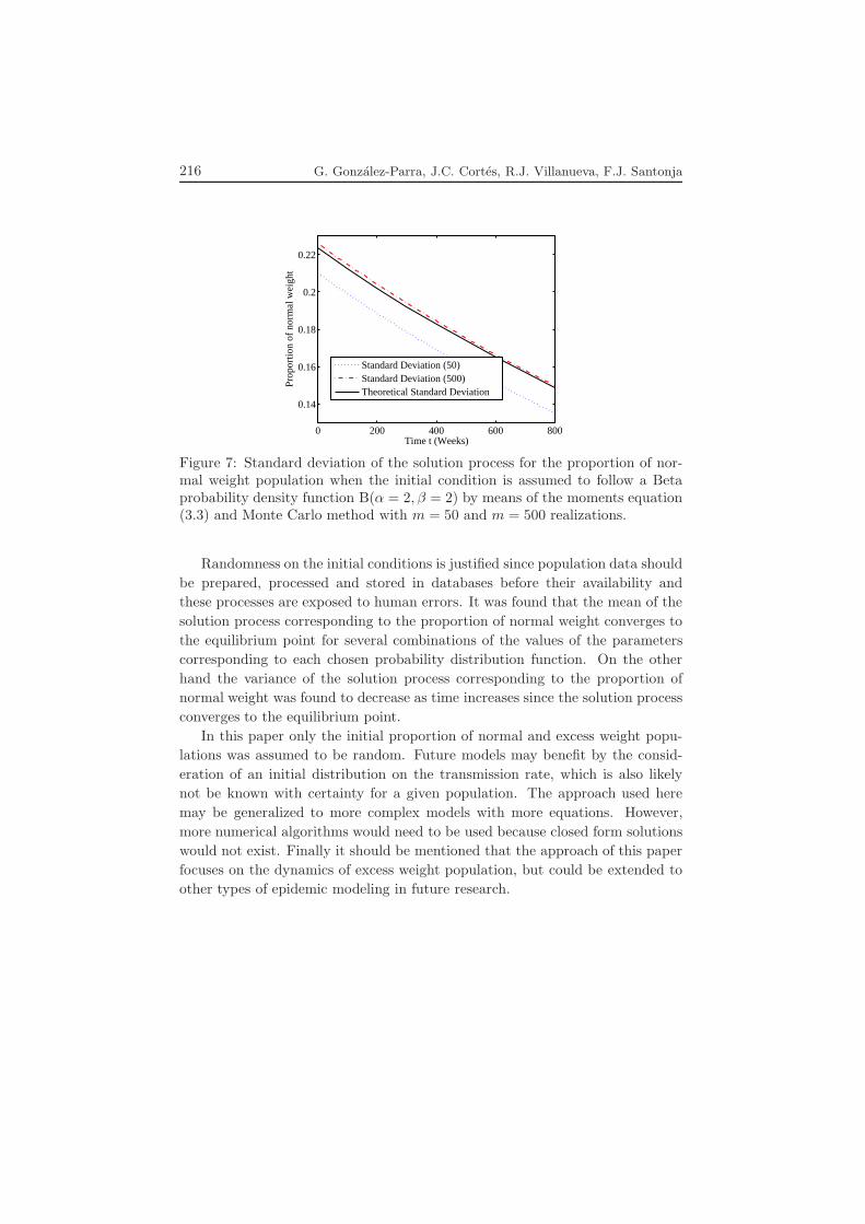
Finally in Figure 7 it can be seen the standard deviation of the solution

process for the proportion of normal weight population when the initial condition

is assumed that follows a Beta probability density function B(α = 2, β = 2).

Numerical results show Monte Carlo method reliability and versatility.

5. Conclusions

In this paper a mathematical model based in the classical SIS epidemic

model was presented in order to predict the evolution of excess weight adult pop-

ulation subject to uncertainty on the initial conditions. The model is represented

by a system of nonlinear differential equations with random initial conditions.

By assuming different probability distribution functions for the initial conditions

of the normal and excess weight populations we obtain the mean and variance of

the stochastic process representing the proportion of normal and excess weight

populations at any time. The mean and variance for each chosen probability

distribution functions are derived by means of the statistical moments equation

and Monte Carlo simulations. The moments equation and Monte Carlo nu-

merical results agree very well. In fact numerical results show that the Monte

Carlo method increases its accuracy as the number of realizations increases as

was expected. The comparisons verify clearly the consistency of the theoreti-

cal approach and the Monte Carlo method as a consequence of the law of large

numbers.


0 1000 2000 3000 4000 50000

0.01

0.02

0.03

0.04

0.05

0.06

0.07

Time t (Years)

Pro

port

ion

of n

orm

al w

eigh

t

Standard Deviation (50)Standard Deviation (500)Theoretical Standard Deviation

Figure 5: Standard deviation of the solution process for the proportion of nor-mal weight population when the initial condition is assumed to follow a Uniformprobability density function on the interval [0.422, 0.622] by means of the mo-ments equation (3.3) and Monte Carlo method with m = 50 and m = 500realizations.

100 200 300 4000.03

0.035

0.04

0.045

0.05

0.055

Time t (Weeks)

Pro

port

ion

of n

orm

al w

eigh

t


Figure 6: Standard deviation of the solution process for the proportion of normalweight population when the initial condition is assumed to follow a truncatedGaussian probability density function with parameters µ = 0.522 and σ = 0.05,on the interval [0.222, 0.822] by means of the moments equation (3.3) and MonteCarlo method with m = 50 and m = 500 realizations.


0 200 400 600 800

0.14

0.16

0.18

0.2

0.22

Time t (Weeks)

Prop

ortio

n of

nor

mal

wei

ght


Figure 7: Standard deviation of the solution process for the proportion of nor-mal weight population when the initial condition is assumed to follow a Betaprobability density function B(α = 2, β = 2) by means of the moments equation(3.3) and Monte Carlo method with m = 50 and m = 500 realizations.

Randomness on the initial conditions is justified since population data should

be prepared, processed and stored in databases before their availability and

these processes are exposed to human errors. It was found that the mean of the

solution process corresponding to the proportion of normal weight converges to

the equilibrium point for several combinations of the values of the parameters

corresponding to each chosen probability distribution function. On the other

hand the variance of the solution process corresponding to the proportion of

normal weight was found to decrease as time increases since the solution process

converges to the equilibrium point.

In this paper only the initial proportion of normal and excess weight popu-

lations was assumed to be random. Future models may benefit by the consid-

eration of an initial distribution on the transmission rate, which is also likely

not be known with certainty for a given population. The approach used here

may be generalized to more complex models with more equations. However,

more numerical algorithms would need to be used because closed form solutions

would not exist. Finally it should be mentioned that the approach of this paper

focuses on the dynamics of excess weight population, but could be extended to

other types of epidemic modeling in future research.


Acknowledgements

The authors are grateful to the anonymous reviewers for their valuable com-

ments and suggestions which improved the quality and the clarity of the paper.

This work has been partially supported by the Spanish M.C.Y.T. and FEDER

grant: MTM2009-08587; FIS PI-10/01433; Universitat Politecnica de Valen-

cia grants: PAID06-11-2070 and PAID-00-11-2753, and Universitat de Valencia

grant: UV-INV-PRECOMP12-80708. First author has been supported by CD-

CHTA project I-1289-11-05-A.

References

[1] Arrizabalaga, J., Masmiquel, L., Vidal, J., Calaas, A., Dıaz, M., Garcıa, P.,

Monereo, S., Moreiro, J., Moreno, B., Ricart, W., and Cordido, F. (2004).

Recomendaciones y algoritmo de tratamiento del sobrepeso y la obesidad en

personas adultas. Med. Clin., 122(3):104–110.

[2] Chen-Charpentier, B., Jensen, B., and Colberg, P. (2009). Random Coef-

ficient Differential Models of Growth of Anaerobic Photosynthetic Bacteria.

ETNA, 34:44–58.

[3] Fishman, G. (1996). Monte Carlo: Concepts, algorithms, and applications.

Springer-Verlag, New York.

[4] Gonzalez-Parra, G., Acedo, L., Villanueva, R.J., and Arenas, A. J. (2010).

Modeling the social obesity epidemic with stochastic networks. Phys. A: Stat.

Mech. Appl., 389(17):3692 – 3701.

[5] Gupta, A. K. (1952). Estimation of the mean and standard deviation of a

normal population from a censored sample. Biometrika, 39(3-4):260–273.

[6] Hanna, S. R., Chang, J. C., and Fernau, M. E. (1998). Monte Carlo estimates

of uncertainties in predictions by a photochemical grid model (uam-iv) due to

uncertainties in input variables. Atmospheric Environ.,, 32(21):3619–3628.

[7] Jodar, L., Santonja, F., and Gonzalez-Parra, G. (2008). Modeling dynamics

of infant obesity in the region of Valencia, Spain. Comput. Math. Appl.,

56(3):679–689.

[8] Ju, S.-J. (2009). On the distribution type of uncertain inputs for probabilistic

assessment. Reliab. Eng. Syst. Saf., 94(5):964 – 968.

[9] Kegan, B. and West, R. (2005). Modeling the simple epidemic with deter-

ministic differential equations and random initial conditions. Math. Biosc.,

195:197–193.


[10] Korsunskii, V. I., Neder, R., Hradil, K., Neuefeind, J., Barglik-Chory, K.,

and Muller, G. (2004). Investigation of the local structure of nanosized cds

crystals stabilized with glutathione by the radial distribution function method.

J. of Struct. Chem., 45(3):427–436.

[11] Mallet, V. and Sportisse, B. (2008). Air quality modeling: From determin-

istic to stochastic approaches. Comput. Math. Appl., 55(10):2329–2337.

[12] Moller, B., Graf, W., Sickert, J.-U., and Steinigen, F. (2009). Fuzzy ran-

dom processes and their application to dynamic analysis of structures. Math.

Comput. Model. Dynamic. Syst., 15(6):515 – 534.

[13] Navarro-Barrientos, J.-E., Rivera, D. E., and Collins, L. M. (2011). A

dynamical model for describing behavioural interventions for weight loss and

body composition change. Math. Comput. Model. Dynamic. Syst., 17(2):183–

203.

[14] Pillards, T., Vandewoestyne, B., and Cools, R. (2010). An adaptive ap-

proach to cube-based quasi-Monte carlo integration on. Math. Comput. Simul.,

80(6):1104 – 1117.

[15] Rasulov, A., Raimova, G., and Mascagni, M. (2010). Monte carlo solution

of Cauchy problem for a nonlinear parabolic equation. Math. Comput. Simul.,

80(6):1118 – 1123.

[16] Santonja, F., Villanueva, R.-J., Jodar, L., and Gonzalez-Parra, G. (2010).

Mathematical modelling of social obesity epidemic in the region of Valencia,

Spain. Math. Comput. Model. Dynamic. Syst., 16(1):23–34.

[17] Soong, T. (1973). Random Differential Equations in Science and Engineer-

ing. Academic Press, New York.

[18] Tuckwell, H. C. and Jost, J. (2009). Moment analysis of the Hodgkin-Huxley

system with additive noise. Phys. A: Stat. Mech. Appl., 388(19):4115 – 4125.

[19] Valencian Department of Health (2000). Health survey, year 2000. Available

at http://www.san.gva.es/val/prof/homeprof.html [Accessed 16 May 2010].

[20] Valencian Department of Health (2005). Health survey, year 2005. Available

at http://www.san.gva.es/val/prof/homeprof.html [Accessed 16 May 2010].

[21] Xiu, D. and Karniadakis, G. E. (2002). Modeling uncertainty in steady

state diffusion problems via generalized polynomial chaos. Comput. Meth.

Appl. Mech. Eng., 191(43):4927 – 4948.


About the authors

Gilberto Gonzalez-Parra is full Professor in the Engineer Faculty of the Uni-

versity of Los Andes (ULA), Merida, Venezuela. He obtained the M.Sc. degree in

Applied Mathematics (University of Los Andes, Venezuela) and the Ph.D. degree

in Applied Mathematics from the University Polytechnic of Valencia, Spain. His

research interests include mathematical epidemiology, numerical analysis, statis-

tical methodology and other areas of applied mathematics.

Juan Carlos Cortes is full Professor in the University Polytechnic of Valencia

(UPV), Spain. He obtained the Ph.D. degree in Applied Mathematics from the

University Polytechnic of Valencia, Spain. His research interests include random

differential equations, mathematical epidemiology, statistical methodology and

options price modeling.

Rafael Jacinto Villanueva is full Professor in the University Polytechnic of

Valencia (UPV), Spain. He obtained the Ph.D. degree in Applied Mathematics

from the University Polytechnic of Valencia, Spain. His areas of interest are

mathematical epidemiology in a wide sense, i.e., not only spread of infectious

diseases, but also spread and transmission of social habits, behavior and ideas.

Francisco Jose Santonja is Professor in the University of Valencia (UV),

Spain at the Statistics and Research operations department. He obtained the

Ph.D. degree in Applied Mathematics from the University Polytechnic of Valen-

cia, Spain. His research interests include mathematical epidemiology, statistical

methodology and calibration and validation of computer models and uncertainty

quatification.

Estad´ıstica Modeling population dynamics with … · Monte Carlo numerical results and the...

Documents

Transcript of Estad´ıstica Modeling population dynamics with … · Monte Carlo numerical results and the...