1

Establishing historical baselines of benthic diversity

and community composition, Western Greenland

Irina Chemshirova

CID: 00643328

Supervisor: Dr Chris Yesson

Word count: 5650

BSc Biology with a Year in Industry/ Research

2

Abstract

Historical data is vital to our understanding of how human-induced changes

affect ecosystems. One of these changes is overharvesting of fish stocks, sometimes

through the means of bottom trawling. This is a major disturbance to the benthos due

to the prolonged contact that fishing gear has with the seabed. It is difficult to find

comparable unimpacted sites in the present day in order to quantify the effect of

trawling. Therefore this study examines historical photographs taken by Per

Kanneworrff (Greenland Institute of Natural Resources) between 1977 and 1984. The

analyses revealed that trawling intensity had negligible effect on the communities

formed. Substrata was found to be the main factor influencing community composition.

We hypothesise that the short window of time (4 years for some stations) we looked at

was not sufficient for any changes due to trawling activity to occur.

Introduction

The human population is growing rapidly and is set to reach 8.9 billion by 2050

(Cohen, 2003). This growth is putting a strain on many ecosystems throughout the

world, with very few still remaining in a truly pristine state. It is very difficult to

quantify the effect we are having on a system after it has been exploited. Therefore we

must turn to historical data. This is an opportunity to re-construct ecosystems to an

unimpacted state, before wide-ranging exploitation began, thus giving us a reference

point for comparison with data collected more recently (Vellend et al., 2013). Swetnam,

Allen & Betancourt (1999) highlight the growing need for pursuing historical data to

determine the processes behind the current patterns and give us some predictive

power for the future. Extensive examination of historical data can also allow us to

avoid shifting the baseline of the ecosystems being studied. A shifting baseline is a

3

phenomenon which occurs when comparisons are drawn between a present day

impacted system with one which has already been significantly degraded (Lotze &

Worm, 2009, Roberts, 2003). When only looking at recent data we also tend to

underestimate the effects that even seemingly primitive methods of exploitation have

had on ecosystems (Pauly, 1995).

Whilst historical data is immensely useful it also presents many challenges. The

datasets are often incomplete. The records can be ambiguous and outdated, using old

taxonomic classifications (Mladenoff et al., 2002). Nonetheless the contribution they

make to our understanding of how the changes imposed upon ecosystems affect them

far outweighs these difficulties.

Historical data is invaluable when attempting to quantify various anthropogenic

effects. For example, it has been used to determine changes in carbon sequestration of

both forests and oceans over time (Rhemtulla, Mladenoff & Clayton, 2009, Cubillos et

al., 2007). Museum collections can often shed light on what an ecosystem looked like in

the past (Hoeksema et al., 2011). Changes in the distribution and population density of

many groups have been studied using various historical sources (Terry, 2010, Skelly et

al., 2003).

We alter much of the environment through the exploitation of populations which

are of economic importance. The Atlantic cod (Gadus morhua) is a classic example.

Rosenberg et al. (2005) have shown, using archaeological records that with increased

fishing pressure the species have decreased in size. Cod is obtained largely through the

means of bottom trawling.

4

Bottom trawling is a fishing practice which has wide ranging impacts on the

ecosystem being exploited. It usually targets organisms that live on the seabed e.g.

crustaceans and demersal fish. This practice is often thought to be highly destructive to

the benthos as the fishing gear is dragged along the seabed. The type of trawl gear used

is of importance when it comes to measuring the fisheries impact. In Western

Greenland, the otter trawl is widely used for the capture of the Northern shrimp

(Pandalus borealis). It typically consists of two trawl doors, (which can weigh up to 5

tonnes each) their function being to keep the net open. Rockhopper gear is an addition

to the otter trawl, developed around 1985. It is made up of bobbins and rollers attached

to the bottom end of the net. It evens out the seabed and dislodges any rocks which may

damage it (Valdemarsen, 2004). Collie et al. (2000) state that dredging has a much

greater impact on the seabed than trawling. Nonetheless, trawling impacts both the

target organism (in this case P. borealis) and the organisms which are caught in the net

as bycatch (Rumohr & Kujawski, 2000). Furthermore there is also the secondary

mortality imposed upon non-target organisms as they are irreparably damaged through

direct physical contact, but not necessarily removing them from their habitat (Jenkins,

Beukers-Stewart & Brand, 2001). Trawling has also been shown to alter nutrient

delivery in the benthic system. Epifaunal organisms receive nutrients in large bursts as

opposed to the usual steady stream (Pilskaln, Churchill & Mayer, 1998).

Jennings et al. (2001) have reported reduced biomass of infaunal and epifaunal

organisms in heavily trawled areas, however they did not find any changes in trophic

structure. Trawling can alter the functional diversity of a community. Tillin et al. (2006)

have shown that with extensive trawling a community shift occurs. From attached filter

feeders towards mobile organisms and infaunal scavengers.

5

The simplification of the habitat which occurs with trawling should not be

underestimated. Much of the complex structures created by sessile organisms such as

soft corals are often levelled out by the trawling gear. Krieger & Wing (2002)

highlighted the importance of these organisms in a benthic ecosystem. They form many

associations with various tropic levels, from predators to animals which seek shelter.

Andrews et al. (2002) also link thriving fish stocks to the presence of healthy Gorgonian

coral gardens.

Considerable changes to the benthic community and its habitat occur after the

first time an area has been trawled (Auster & Langton, 1999). Many studies attempting

to quantify the effects of trawling in the present day are dealing with a system which

has already undergone considerable change (Garcia, Ragnarsson & Eiríksson, 2006).

Therefore this study focuses on historical image data from 1977 until 1984.

According to Hamilton, Brown & Rasmussen (2003) the west Greenlandic

fishery primarily exploited G. morhua until the early 1970s through the means of

bottom trawling until the stock eventually crashed. It has been recorded that a

movement form G. morhua to P. borealis occurred around 1972 when catches were

estimated at 10 tonnes a year (Figure 1).

Figure 1. Showing the biomass of the cod and shrimp catch of the West Greenland fishery 1950 - 2000, Adapted from Hamilton, Brown & Rasmussen (2003).

6

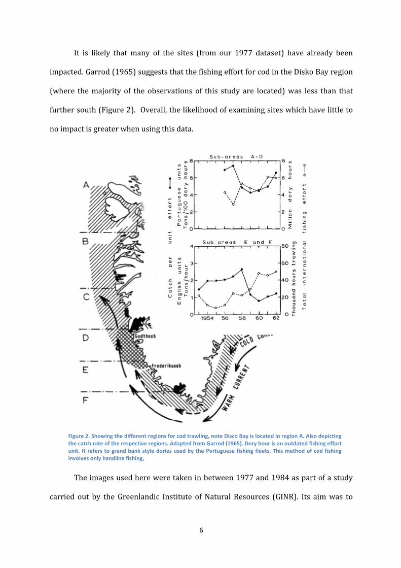
It is likely that many of the sites (from our 1977 dataset) have already been

impacted. Garrod (1965) suggests that the fishing effort for cod in the Disko Bay region

(where the majority of the observations of this study are located) was less than that

further south (Figure 2). Overall, the likelihood of examining sites which have little to

no impact is greater when using this data.

The images used here were taken in between 1977 and 1984 as part of a study

carried out by the Greenlandic Institute of Natural Resources (GINR). Its aim was to

Figure 2. Showing the different regions for cod trawling, note Disco Bay is located in region A. Also depicting the catch rate of the respective regions. Adapted from Garrod (1965). Dory hour is an outdated fishing effort unit. It refers to grand bank style dories used by the Portuguese fishing fleets. This method of cod fishing involves only handline fishing,

7

estimate the density of the shrimp population without the need for survey trawls

(Kanneworff, 1978) . This is an opportunity to observe what the seabed looked like

before large-scale trawling has occurred.

This project aims to compare data obtained from these images in the 1970s and

the 1980s. The 70s dataset will serve as a pre-intensive fishing baseline to compare

with the 80s dataset.

We also aim to collect data from a single year of the historical dataset (1984)

and use the historical trawling effort data available (1975 to 1984), in order to see if a

relationship can be inferred.

Materials and Methods

Kanneworff (1979) used a 35 mm robot camera with a flash and power unit in

waterproof housing to take the images processed here. The equipment was lowered to

the seabed using a winch wire, an image was taken once every minute after the bottom

sensor detected the seabed.. The equipment was allowed to drift whilst the ship

followed it using its echolocation system. The total area of an image is 3.39 m2

Much biodiversity and community analysis is dependent on correct taxonomic

identification. Therefore two datasets will be generated. One which contains organisms

identified to various taxonomic levels (e.g. some at order others at family level

Appendix 1.1) and another in which all are at the Class level (Appendix 1.2). This aims

to check how a variety of taxonomic levels may influence the statistical analysis.

8

The camera film was provided by GINR. It consisted of 56 reels of Kodak Safety

Film 5036 (ISO 400), spanning from 1975 until 1986. Location data was not available

for the stations from 1975 and 1976 and therefore could not be used. Using the location

data provided, the rest of the stations were placed on a map using QGIS (Figure 3).

Figure 3. Map of the stations used in this study, showing the cumulative amount of trawling occurred in the area between 1975 and 1984. This area overlaps with regions A and B for cod fishing (Figure 2)

9

The Kanneworff team aimed to visit the same stations each year of their survey,

however due to poor weather conditions this was not always possible. For two stations

to be regarded as a pair they can be a maximum of 5 km apart.

We combined the images from 1977, 1978, 1979 and 1980 to make the 70s pre-

intensive fishing dataset as this allowed for the largest number of paired stations (19 in

total) thi allowed for a minimum 4 year gap for most stations. The relevant stations

form the 1984 reels were used for the 1980s data. All 36 stations from 1984 were

digitized.

Ten images were digitized from each of the chosen stations using a Reflecta i-

scan 3600 at a resolution of 3600 dpi to ensure high image quality. An air duster

containing 1, 1, 1, 2 – Tetrafluroethane was frequently used to limit the dust particles

which can reduce image quality. The batch- processing function in Photoshop Elements

8 was used to improve image sharpness and colour. A total of 567 images were

digitized, only 295 (five per station) were processed, with the best quality images being

chosen for each station.

Image Processing

The processing of an image usually involves identifying an organism and

counting how many of it were present in the current image. Most of the identifications

were made based on prior knowledge of the study system. An ID guide was compiled in

2013 in order to facilitate processing of the 2011-2013 image data collected for the

same region (Appendix 1.3), this was referred to in case of doubt. As the image quality

was sometimes not as high as desired some taxa were counted as “unkown”. This

classification was used for organisms which were deemed alive but the image was not

10

high quality enough to allow for the distinction of any defining feature. Sensitive taxa

were also noted as organisms which are upright and thus more vulnerable to damage

from the trawl gear (Appendix 1.1 highlights which taxa were classed as sensitive)(de

Juan, Demestre & Thrush, 2009). After all of the organisms visible in the image were

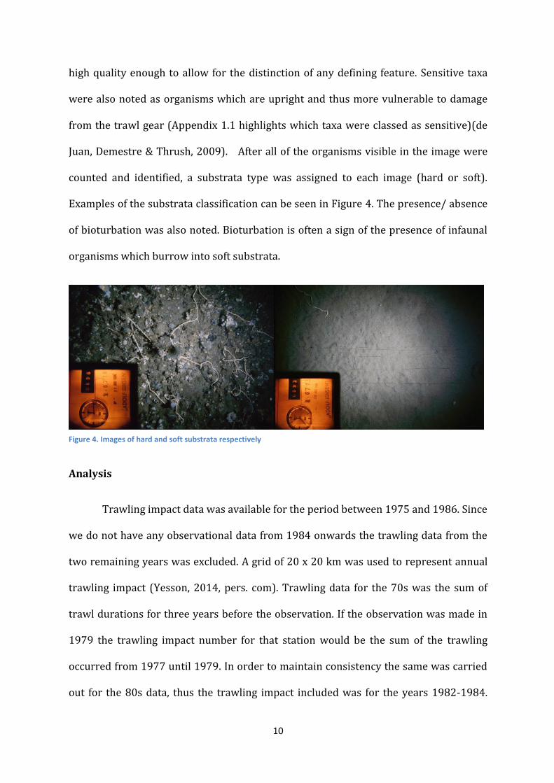
counted and identified, a substrata type was assigned to each image (hard or soft).

Examples of the substrata classification can be seen in Figure 4. The presence/ absence

of bioturbation was also noted. Bioturbation is often a sign of the presence of infaunal

organisms which burrow into soft substrata.

Analysis

Trawling impact data was available for the period between 1975 and 1986. Since

we do not have any observational data from 1984 onwards the trawling data from the

two remaining years was excluded. A grid of 20 x 20 km was used to represent annual

trawling impact (Yesson, 2014, pers. com). Trawling data for the 70s was the sum of

trawl durations for three years before the observation. If the observation was made in

1979 the trawling impact number for that station would be the sum of the trawling

occurred from 1977 until 1979. In order to maintain consistency the same was carried

out for the 80s data, thus the trawling impact included was for the years 1982-1984.

Figure 4. Images of hard and soft substrata respectively

11

The trawling impact data for both time periods was treated as a continuous explanatory

variable. Shapiro – Wilks test was carried out on both datasets to assess if they were

normally distributed. Both failed the normality test (W=0.48, p<0.001 for 1970s and

W=0.63, p<0.001 for the 1980s). Therefore both were log transformed to the base of e.

After the transformation was carried out the data was again tested for normality, and it

failed (W=0.83, p<0.01 and W=0.85, p<0.01 for the 70s and 80s respectively). However

as this improved the distribution of the data, the log transformed version was used for

the analysis.

Historical comparisons

Species accumulation curves for each time period were composed in order to

asses if the sampling effort was sufficient (Ugland, Gray & Ellingsen, 2003).

The following diversity measures were calculated for each station: taxon

richness (α diversity), number of individuals, Pileou’s evenness and the Shannon-

Weiner Index. It is a composite measure attempting to combine both richness and

evenness of the community, it was calculated using Eq1.

∑

Pileou’s evenness was calculated using the H’ derived from the Shannon-Weiner Index,

Eq 2. It attempts to quantify how equal the community is and thus acts as a correction

factor for the Shannon – Weiner Index.

(Eq. 1)

12

All diversity measures were treated as continuous response variables. Scatter

plots of the different diversity indices from both periods against one another were

produced in order to visualise what changes may have occurred.

Wilcoxon signed-rank paired tests were performed in order to determine if

there is any significant difference in the diversity measures between the two time

periods. The changes in taxon richness were visualised using QGIS, where a map

showing the increase or decrease in richness was produced with the relative fishing

intensity. .

Non - metric Multi-dimensional Scaling (nMDS) is an ordination representing the

variation in community composition in a reduced number of dimensions. It has been

used to visualise the community composition of both time periods. Environmental

vectors were overlaid onto this analysis to determine if they can provide an explanation

of patters observed. The environmental vectors included in the analysis were: Latitude,

Longitude, Depth, Fishing (Trawling) Impact, Substrata and Bioturbation.

A hierarchical cluster analysis was also performed in order to compare and

contrast the patterns highlighted by the nMDS analysis. This classifies the different

stations based on the number of dissimilarities between them using Euclidian distance

as a measure. A dendogram using the complete clustering method was generated for

the data from both historical periods.

(Eq. 2)

13

A linear regression of taxon richness and trawling impact was carried out to

determine if there is a relationship. Both time periods were plotted on the same scatter

plot.

β diversity has been calculated using the Bray – Curtis dissimilarity method to

quantify the diversity change over time. This takes into account that, diversity indices

may not vary between the two time periods but the taxon identities might i.e. a shift

from soft corals to decapods. A linear regression was carried out to determine if

trawling impact affects the amount of change observed. A high number of β diversity

indicates a large change in the taxon identities.

Historical comparisons – Class level

All of the analyses described were then repeated for the dataset in which all

organisms are identified at the Class level.

Single year historical dataset (1984)

Further analysis was also pursued with the 1984 dataset. The same diversity

indices were calculated. A linear regression was performed to determine if there is a

relationship between trawling impact and diversity. nMDS and cluster analyses were

also performed. The ward method was used for the clustering of this dataset. A species

accumulation curve was also estimated.

With these additional analyses, many of the results did not differ from the initial

historical comparison. Therefore they have been placed in the Appendix.

All analysis was performed using the statistics software R and the following

packages: vegan and plyr (R Core Team, 2013, Oksanen et al., 2013, Wickham, 2011).

14

Results

Historical comparisons

For the comparison between the 70s and the 80s 19 stations were processed,

giving a total of 38. Overall 38 taxa were identified across both time periods, including

an additional classification for “unknown” organisms. Encrusting bryozoa was the most

abundant taxon in both time periods. Overall out of the five most numerous taxa, three

belonged to the sensitive taxa group (Figure 5). Sabellidae and ascidians were found to

decrease in abundance over time. Brittle stars, soft bryozoans, stylasterina, serpulidae

and soft coral on the other hand have increased over time (Appendix 1.4).

PterasteridaePolynoidae

IsopodaSea SpidersScaphopods

ScorpaeniformesAstropectinidae

Sea UrchinsEunicidae

RajiformesCrinoidsBivalves

AsteriidaeStarfish Other

GastropodsSea Cucumbers

GoniasteridaeZoanthids

EchinasteridaeTerebratulida

PleuronectiformesHydroids

PerciformesSoft CoralsSabellidaeAnemones

UnknownSerpulidae

Arborescent SpongesStylasterinaBrittlestars

Encrusting SpongesSoft Bryozoa

Massive SpongesDecapoda

Erect BryozoaAscidians

Encrusting Bryozoa

Total

0 200 400 600 800

Figure 5: Shows the taxa identified and their relative abundance for the 70s and 80s datasets. Sensitive taxa have been highlighted

15

The species accumulation curve produced showed that increasing the sampling

effort would not lead to new undiscovered taxa being added (Figure 6). This was also

separetly performed for the two time periods and showed the same pattern (Appendix

1.5). The chao method estimated that there should be 41 taxa (SE=3), whilst we found

38.

0 10 20 30

01

02

03

04

0

Sites

Ta

xa

Figure 6. Shows the curve beginning to asymptote suggesting that the sampling is sufficient.

16

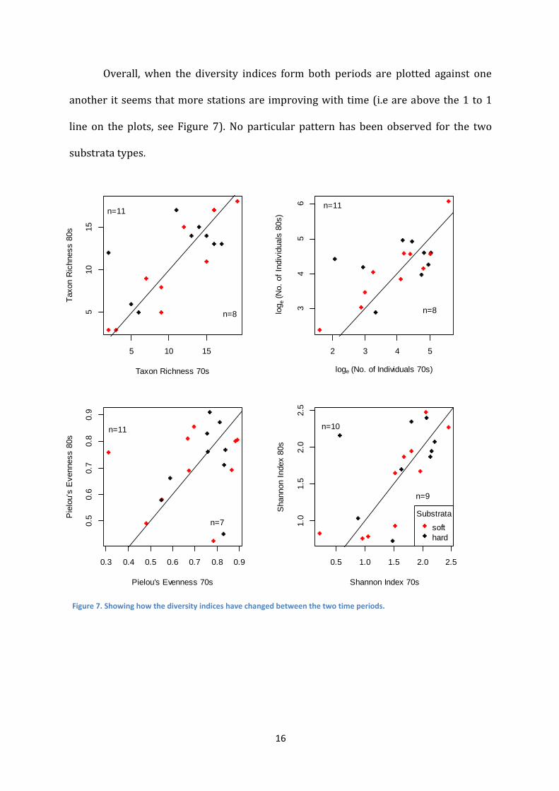
Overall, when the diversity indices form both periods are plotted against one

another it seems that more stations are improving with time (i.e are above the 1 to 1

line on the plots, see Figure 7). No particular pattern has been observed for the two

substrata types.

Figure 7. Showing how the diversity indices have changed between the two time periods.

5 10 15

510

15

Taxon Richness 70s

Taxon R

ichness 8

0s

n=11

n=8

2 3 4 5

34

56

loge (No. of Individuals 70s)

log

e(N

o.

of

Indiv

iduals

80s)

n=11

n=8

0.3 0.4 0.5 0.6 0.7 0.8 0.9

0.5

0.6

0.7

0.8

0.9

Pielou's Evenness 70s

Pie

lou's

Evenness 8

0s

n=11

n=7

0.5 1.0 1.5 2.0 2.5

1.0

1.5

2.0

2.5

Shannon Index 70s

Shannon I

ndex 8

0s

Substrata

soft

hard

n=10

n=9

17

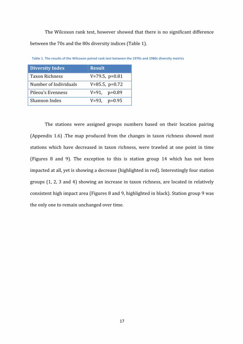
The Wilcoxon rank test, however showed that there is no significant difference

between the 70s and the 80s diversity indices (Table 1).

Diversity Index Result

Taxon Richness V=79.5, p=0.81

Number of Individuals V=85.5, p=0.72

Pileou’s Evenness V=91, p=0.89

Shannon Index V=93, p=0.95

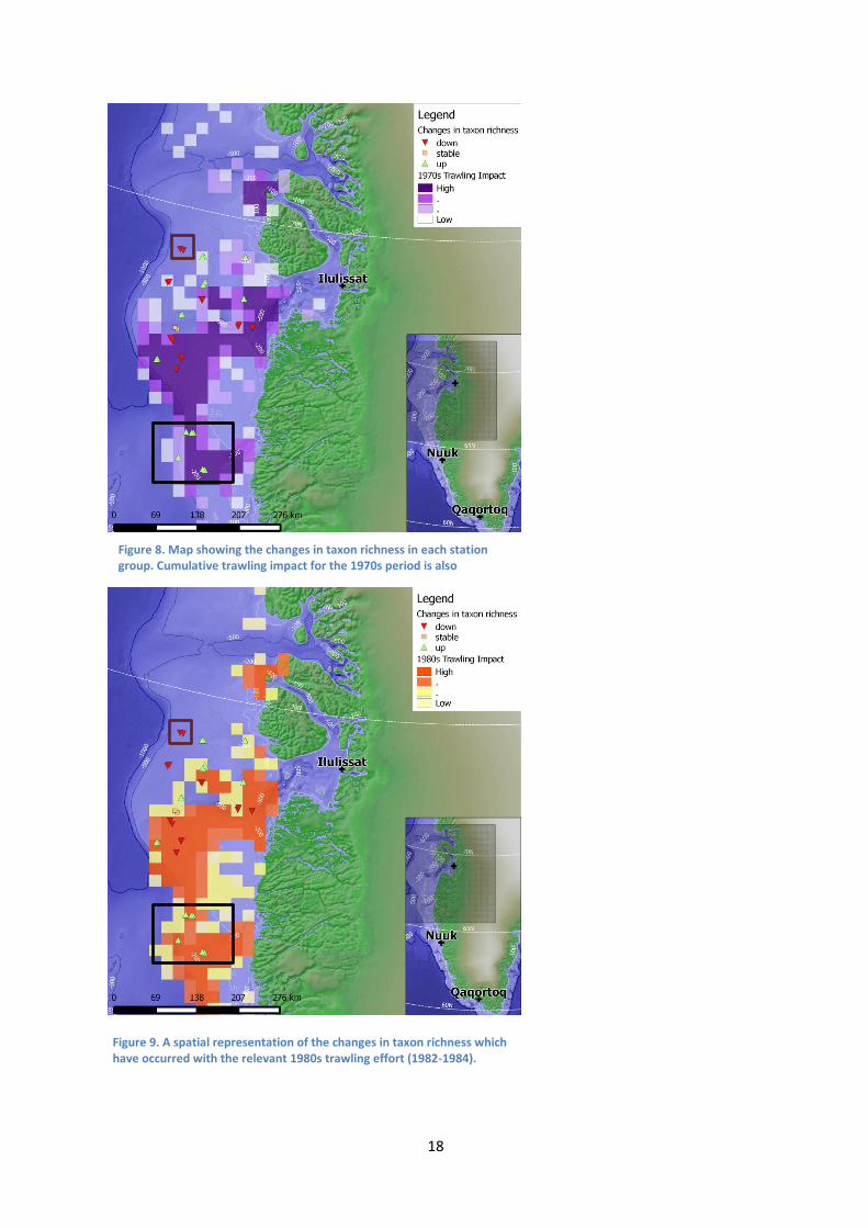
The stations were assigned groups numbers based on their location pairing

(Appendix 1.6) .The map produced from the changes in taxon richness showed most

stations which have decreased in taxon richness, were trawled at one point in time

(Figures 8 and 9). The exception to this is station group 14 which has not been

impacted at all, yet is showing a decrease (highlighted in red). Interestingly four station

groups (1, 2, 3 and 4) showing an increase in taxon richness, are located in relatively

consistent high impact area (Figures 8 and 9, highlighted in black). Station group 9 was

the only one to remain unchanged over time.

Table 1. The results of the Wilcoxon paired rank test between the 1970s and 1980s diversity metrics

18

Figure 8. Map showing the changes in taxon richness in each station group. Cumulative trawling impact for the 1970s period is also represented.

Figure 9. A spatial representation of the changes in taxon richness which have occurred with the relevant 1980s trawling effort (1982-1984).

19

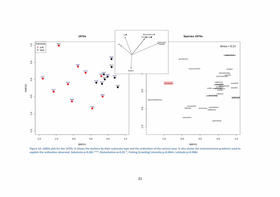
Diversity indices such as these however reveal little in the way of the various

communities in the area. Therefore we carried out nMDS plots which reveal the

relevant communities for both time periods.

In the 1970s substrata was shown to be an important factor in differentiating

between the two communities observed in the nMDS plot (p=0.001, ***, Figure 10).

The other environmental vectors overlaid on the nMDS plots highlighted that

substrata type has a very strong influence on the community composition of the 1970s.

Interestingly, for the 1970s period, trawling effort appears to have a greater impact on

hard substrata. Considering the species plot, decapods (which primarily consist of P.

borealis, the target species of the fishery) appear to not be affected by the trawling

(Figure 10, highlighted in red). Trawling impact has shown to have very little influence

on the community composition (p=0.064, •) along with Latitude (p=0.098, •).

Bioturbation also had some effect, in a different direction to substrata type (p<0.05,*).

Depth and Longitude were not shown to explain any of the observed variation.

For the 1980s only substrata explained the patterns observed in the nMDS plot

(p=0.001, ***, Figure 11). In this species plot, decapods appeared where expected with

respect to trawling (Figure 11, highlighted in red).

An alternative approach to viewing the relationships between stations in terms

of communities is a cluster analysis. This method uses a dendogram to show how the

stations cluster together based on the taxa they contain. It showed some stations which

were designated as hard substrata in the soft substrata cluster (Figure 12). In the hard

substrata cluster (highlighted in black, Figure 12), the dominant taxa were encrusting

sponges and bryozoans along with ascidians and soft corals. In the soft substrata cluster

20

(highlighted in red, Figure 12) decapods were found to be most numerous. Stations

5606 and 6716 (group 3) have been shown to be very different in terms of their

composition compared to the other stations (highlighted in green, Figure 12). Many of

the stations occur very far from their paired station in the dendogram, e.g. 5605 and

6720 (group 4, highlighted in blue, Figure 12). It is also worth noting that many stations

pairs which have been placed in the same substrate cluster are still described as quite

different from one another e.g. 5609 and 6713, group 1, highlighted in purple, Figure

12.

21

-1.5 -1.0 -0.5 0.0 0.5 1.0

-1.5

-1.0

-0.5

0.0

0.5

1.0

1970s

NMDS1

NM

DS

2

5609

5453

5606

5605

5601

5739

5447

5867

5612

5613

5743

5738

5870 5869

5871

5859

5444

5861

5737

Substrata

soft

hard

-1.0 -0.5 0.0 0.5 1.0-1

.0-0

.50

.00

.51

.0

Species 1970s

NMDS1

unspecified

softcoral

anemones

zoanthids

hydroids

stylasterinapterasteridae

echinasteridae

goniasteridae

astropectinidae

starfishother

brittlestars

seaurchins

seacucumbers

crinoids

encrustingsp

massivesparborescentsp

sabellidae

serpulidaem

polynoidae

decapoda

isopoda

gastropods

bivalves

terebratulida

erectbrencrustingbrsoftbr

ascidians

rajiformes

perciformes

pleuronectiformes

NMDS1

NM

DS

2

X1

Y1

Depth1

Fishing.Log

Substrata1

Bioturbation1

*

***

• •

Figure 10. nMDS plot for the 1970s. It shows the stations by their substrata type and the ordination of the various taxa. It also shows the environmental gradients used to explain the ordination observed. Substrata p<0.001 ***, Bioturbation p<0.05 *, Fishing (trawling) intensity p=0.064•, Latitude p=0.098•

Stress = 0.13

22

-1.0 -0.5 0.0 0.5 1.0 1.5

-1.0

-0.5

0.0

0.5

1.0

1980s

NMDS1

NM

DS

2

6713

6715

6716 6717

6720

6721

6722

6724

6727

6728

6729

67306731

6732

6733

6736

6737

6738

6749

Substrata

soft

hard

-0.5 0.0 0.5 1.0 1.5

-0.5

0.0

0.5

1.0

1.5

Species 1980s

NMDS1

unspecified

softcoral

anemoneszoanthids hydroids

stylasterina

asteriidae

echinasteridae

goniasteridae

astropectinidae

starfishother

brittlestars

seacucumbers

encrustingsp

massivesp

arborescentspsabellidae

eunicidae

serpulidaemdecapoda

seaspiders

gastropods

bivalves

scaphopods

terebratulida

erectbr

encrustingbr

softbr

ascidians

rajiformes

scorpaeniformes

perciformes

pleuronectiformes

NMDS1

NM

DS

2

X2

Y2

Depth2

Fishing.LogSubstrata2

Bioturbation2

***

Figure 11. nMDS plot for the 1980s. It shows the stations by substrata type and the ordination of the various taxa. It also shows the environmental gradients used to explain the ordination observed - Substrata p<0.001 ***

Stress = 0.14

23

67

37

67

33

56

05

67

13

58

67

67

24

67

28

67

49

56

13

57

37

67

21

67

29

54

44

56

09

57

43

56

12

58

61

67

27

57

38

58

70

67

38

58

59

67

30

67

31

58

71

54

47

56

01

58

69

67

15

67

32

54

53

67

22

57

39

67

20

67

17

67

36

56

06

67

16

05

01

00

15

02

00

Cluster Dendrogram

hclust (*, "complete")

all.dist

He

igh

t

Figure 12. Dendogram of the hierarchical clustering. Highlighted in red are the stations with a soft substrata classification, stations highlighted in black classed as hard substrata. Stations with an * beside them are classed as hard substrata but have been grouped with the soft by the analysis. The numbers below denote the station groups based on their location.

17 15 4 1 8 8 10 19 10 19 6 11 17 1 11 9 18 9 12 13 18 16 12 13 15 7 5 14 2 14 2 7 6 5 4 16 3 3

* * *

24

No relationship could be inferred between increasing trawling intensity and

taxon richness. Linear regressions for both the 1970s and 1980s showed no particular

patterns in terms of positive or negative effects of increasing trawling intensity on

taxon richness (Figure13).

There is no relationship between β diversity and trawling pressure as shown by

the linear regression in Figure 14.

0 2 4 6 8 10 12

51

01

5

loge (Trawling Impact 1975-1984)(mins)

Ta

xo

n R

ich

ne

ss

hard

soft

1970s

1980s

Figure 13. Showing the relationship between trawling intensity and taxon richness. Trawling has no effect on taxon richness for the 1970s period (t=1.4, d.f.=17, p=0.17). There is no relationship between trawling impact and taxon richness for the 1980s (t=0.3, d.f.=17, p=0.54).

25

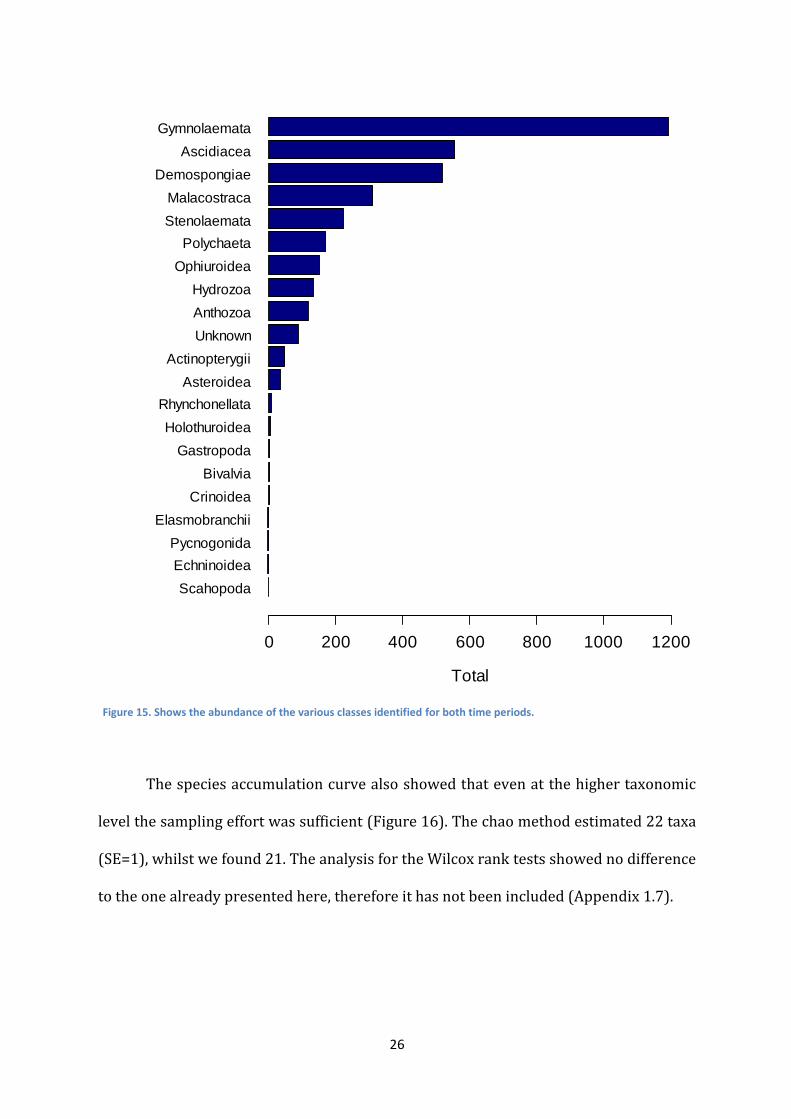
Historical comparisons – Class

The class level analysis was performed because community and diversity indices

can often be influenced by the level of taxonomic resolution used for the identification

of organisms. Bryozoa were still the most abundant of taxa (Gymnolaemata) at class

level, followed by Ascidiacea and Demospongiae (Figure 15).

0 2 4 6 8 10

0.2

0.3

0.4

0.5

0.6

0.7

loge (Trawling Impact 1982-1984)(mins)

Be

ta D

ive

rsity

Substrata

hard

soft

Figure 14. Showing the relationship between β diversity and trawling impact. Increasing trawling impact had no effect on the β diversity observed (t=0.77, d.f.=17, p=0.45)

26

The species accumulation curve also showed that even at the higher taxonomic

level the sampling effort was sufficient (Figure 16). The chao method estimated 22 taxa

(SE=1), whilst we found 21. The analysis for the Wilcox rank tests showed no difference

to the one already presented here, therefore it has not been included (Appendix 1.7).

Scahopoda

Echninoidea

Pycnogonida

Elasmobranchii

Crinoidea

Bivalvia

Gastropoda

Holothuroidea

Rhynchonellata

Asteroidea

Actinopterygii

Unknown

Anthozoa

Hydrozoa

Ophiuroidea

Polychaeta

Stenolaemata

Malacostraca

Demospongiae

Ascidiacea

Gymnolaemata

Total

0 200 400 600 800 1000 1200

Figure 15. Shows the abundance of the various classes identified for both time periods.

27

The nMDS plots for both periods showed that substrata type is the most

important environmental factor governing the community composition (Appendix 1.8).

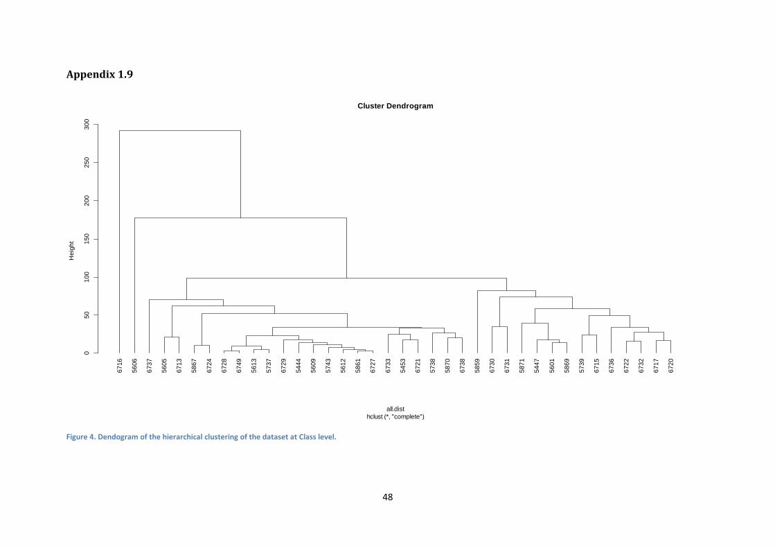
The cluster analysis mostly maintained the main patterns observed in the

previous dataset (Appendix 1.9). The linear regressions carried out for the taxon

richness and β diversity again were unaffected by increasing trawling intensity

(Appendix 2.0 and 2.1 respectively).

0 10 20 30

51

01

52

0

Sites

Ta

xa

Figure 16. The number of new taxa being identified is shown to asymptote with increasing sampling effort.

28

Single year historical dataset (1984)

The species accumulation curve again showed that increased sampling effort

would unlikely uncover additional taxa (Appendix 2.2). Chao estimate stated that there

could be 40 taxa (SE=3), we found 38. The nMDS plots revealed substrate to be the most

important environmental factor in the community composition (Appendix 2.3).

Cluster analysis revealed three clusters. Cluster A contained true hard substrata

stations (Figure 17). Cluster B contained mainly soft substrata stations. Cluster C was

designated as mixed as it contained an equal number of hard and soft substrata

stations. Two stations were notably different from all the rest – 6716 and 6743

(highlighted in orange, Figure 17).

Linear regression analysis found that trawling intensity has no effect on taxon

richness in the 1984 dataset (Appendix 2.4).

29

67

42

67

44

67

48

67

20

67

17

67

36

67

14

67

25

67

23

67

21

67

26

67

29

67

19

67

41

67

27

67

34

67

28

67

49

67

38

67

24

67

40

67

30

67

31

67

46

67

18

67

37

67

15

67

35

67

22

67

32

67

45

67

47

67

13

67

33

67

16

67

43

02

00

40

06

00

80

0Cluster Dendrogram

hclust (*, "ward")

dist84

He

igh

t

* * * * *

Figure 17. A dendogram showing the 3 distinct clusters, referred to A, B and C respectively left to right.

30

Discussion

The number of taxa identified did not differ significantly when compared to

other studies. Jones, Bett & Tyler (2007) studied the megabenthos off the coast of East

Greenland and found 45 taxa at varying taxonomic levels through the means of bottom

photography. Whilst Cusson, Archambault & Aitken (2007) found 68 orders and 29

classes, when examining historical records from 1955 – 1977. The area they examined

was much larger, from Beaufort Sea in the west to the Southern Davis Strait in the west.

In terms of abundance, we found that the numbers of soft corals increased with time,

whilst Strain et al. (2012) found a decline. The Strain study was at a relatively shallow

depth (30m). They also had a temporal gap of 24 years compared to a minimum 4-year

gap in our study. Both of those factor may have contributed to the discrepancies with

our results. The increase of soft coral with time we have observed is a curious

phenomenon as they are vulnerable to fishing gear as they cannot escape it as easily as

mobile taxa. Looking back at the specific images where they were found the 70s dataset

contains more large soft corals than the 80s one. There was also an increase in brittle

stars, which have been classed as sensitive to trawling by Olsgard et al. (2008). The

reason for this dissimilarity could be that they have a different functional role in this

community e.g. as scavengers as opposed to filter feeders.

We did observe a slight decline in ascidian abundance, which is in line with

Strain’s (2012) findings. Sabellidae worms decreased in abundance greatly. Simpson &

Watling (2006) found a similar abundance pattern in the gulf of Maine when comparing

trawled and untrawled areas.

No significant change was observed in the diversity indices between the

two time periods. This would suggest that the communities have remained relatively

31

stable over the 4-year period. Kenchington et al. (2007) found little variation in species

richness when comparing two time periods with a 30-year gap. However their study

was based in the Bay of Fundy, Canada which is quite sheltered. This could be the

reason they did not see difference.

When the changes in richness are placed on a map, several station groups show

interesting patterns. Station group 14 (highlighted in red, Figures 8 and 9) is the most

curious one by far. It shows a decrease in both richness and number of individuals, yet

it has not experienced any trawling activity. When looking at this group closely it, the

80s station has only one taxon less than the 70s one. This is due to rare taxa, more

specifically Pterasteridae as it only appears once in the whole dataset, in that station. It

is therefore possible that the analyses are skewed due to rare taxa. Some studies have

excluded taxa with abundance lower than 5%, this would be something to consider

testing out for this study in the future (Frid et al., 2000). Four stations increased in

richness over time even though the area was heavily trawled in the four-year period.

Hill et al. (1999) suggest that this could be due to trawling activity sometimes bringing

up more stones to the surface creating more opportunities for colonisation by sessile

organisms. Diversity indices show if there has been a significant change in terms of

number of taxa but do not highlight how the community composition has changed.

Therefore we carried out an nMDS analysis.

The nMDS plot for the 1970s period reveal two main communities, one

associated with soft substrata and another with hard substrata. The environmental

vectors also highlighted the same pattern as substrata type being a significant driver in

determining the composition of the stations. Kenchington et al. (2007) show a much

weaker substrata effect in a similar analysis. The communities seemed to be largely

32

differentiated by the time period they belonged to as opposed to substrata.

Kenchington et al. (2007) attributed this to dredging and trawling activity occurring

between 1967 and 1997 changing the community composition. The area they

investigated was at depths between 100-200m so it is very likely that a different

community is concerned to the one this study has sampled. When both time periods

were plotted for this study, no pattern was observed (Appendix 2.5).

Bioturbation also affected community structure, this is likely to be due to the fact

that soft substrata is inhabited by infaunal and burrowing organisms which modify the

sediment regularly. However, this does not point in the same direction as substrata

which is unexpected, it seems to overlap with the fishing effort variable instead.

The trawling effort is giving a weak signal in terms of community structure. It is

possible that the strong substrata signal is masking the effect fishing is having on the

communities. Kaiser et al. (1998) analysed communities separately after they

concluded that there was a significant difference between the two due to substrata

type. This is something to consider if developing this project further. Another

possibility for the apparent lack of fishing influence on communities is the quality of the

fishing data itself. This dataset only includes one location for the trawls, i.e. it could be

start or end. Therefore a coarse grid of 20 x 20 km needed to be used in order to

account that an average trawl could be of length of 20 km. This means that the data is of

a relatively low resolution. Stations within the 20km square will show the same amount

of impact even if the trawl has not passed through there. Bradshaw, Veale & Brand

(2002) had a relatively poor quality fishing dataset when comparing benthic

community data from 1938-1950 with that from 1990. They attempted to solve this

issue by creating several proxies for fishing impact. The two that showed changes

33

between the communities were “number of years since first fished” and a “Fishermen’s

Index”. The number of years is a count of how long an area has been exploited. The

Fishermen’s Index was developed by conferring with local fishermen on how intensive

the fishing has been in the area by giving a score from 1 (being low) to 7 (being high).

Both of those methods for quantifying fishing effort would be interesting and possibly

more realistic alternatives to the current dataset.

It is possible that the cod fishery, which was active in the area almost 60 years

before the images were taken, has had a greater impact on the benthos than

anticipated. Therefore, the change which we are trying to quantify may have already

happened. We may be sampling a system in an already degrading state, thus shifting the

baseline.

When looking at the position of certain taxa in the nMDS plot it is strange to see

that the decapods were ordered with taxa at stations which are less affected by

trawling, This however, could still be the substrate effect, as the soft substrata were

trawled less intensively on average.

The 1980s MDS ordination showed similar patterns to the 1970s with one

notable difference. Substrata was the only environmental variable to explain the

communities observed. The fact that fishing did not have an effect was expected

because the initial impact should have been obvious in the first time period (70s) as the

initial impact on a community is often the greatest. Even though the effect of fishing

was negligible, decapods were placed where expected with respect to fishing.

The cluster analysis reinforced the main message of the nMDS analysis, that

substrata is the main factor determining the communities in this study. Kaiser et al.

34

(2002) described the importance of the sediment type when considering the effect

trawling may have on the benthos. Three stations which have been classed as hard have

however clustered with the soft substrata stations (6733, 6721 and 5738). The reason

for this is likely to be that these stations were relatively impoverished and contained a

few individuals from taxa generally associated with soft substrata e.g. decapods and

serpulids. Two stations (5606 and 6716) were very distinct from any of the other

stations and form one another. When the images from the stations were examined, it

was obvious that they were quite different substrata, being mostly large boulders with

few organisms. Considering the different station groupings it was surprising to see that

stations which have similar locations (within 5 km) would appear so far away from one

another in the dendogram e.g. group 4. When their substrata class was taken into

account the difference in clustering was likely because one station was soft substrata

and the other hard substrata. However groups which have been given the same

substrate classification e.g. group 1 have also occurred on distant branches on the

dendogram. This difference could be attributed to trawling pressure, as effort was

shown to increase for that station. It is worth noting that fishing effort is often patchy

thus it can be difficult to pin-point if the increase in effort occurred evenly in the 20 x 20

km square or if only a stretch of a few kilometres was affected (Cryer, Hartill & O'shea,

2002).

Linear regressions of trawling against taxon richness showed no relationship.

Separating out the different time periods had the same result. Although a non-

significant positive slope can be seen for the 1970s. This however is a substrate effect

again (Kaiser et al., 1998). It can be inferred from this that on average hard substrata

are more taxon rich than soft substrata.

35

β diversity showed no relationship, but it can be argued that overall soft

substrata have been subject to grater changes in the identities of species. One likely

reason for the lack of pattern observed in the regressions is the quality of the trawling

data.

The analysis performed at the Class level showed no major differences from the

data at various taxonomic levels. Therefore, our choice of taxon categories were similar

to choosing a consistent class level grouping. It is possible that more specific

identification e.g. genus would change our results. Nonetheless this is not realistic or

possible for many of the organisms when collecting data from images. Many taxa (e.g.

Porifera) need to be examined under a microscope in order to be assigned a more

specific taxonomic classification.

The analysis carried out on the 1984 data only, again differed little from the

original one. The only real difference was in the cluster analysis. Instead of forming two

distinct clusters, three were formed. Two were deemed hard and soft, whilst a third one

could be described as mixed. This could be due to the different clustering method used.

Two stations again showed to differ from the rest of the stations – 6716 and 6743. The

reasons for this are the same as pointed out earlier.

The main outcome of this study is that substrata is the key variable in

determining the communities in the Greenlandic benthos. It is possible that the effects

of trawling were not apparent in this study because the 4-year window is not enough

for the effects of trawling to truly manifest themselves. Processing more images per

station may give us a better idea of the community composition of this area. It would

also be interesting to compare present date image data with the historical data. Then

the community changes may become more apparent.

36

Acknowledgments

I would like to thank Kirsty Kemp and Chris Yesson at the Institute of Zoology for the

extensive help and guidance throughout this project. Many thanks to Henrik Lund at the

Greenland Institute of Natural Resources for alerting us to the existence of the historical

images and GINR for kindly providing them.

References

Andrews, A. H., Cordes, E. E., Mahoney, M. M., Munk, K., Coale, K. H., Cailliet, G. M. & Heifetz, J. (2002) Age, growth and radiometric age validation of a deep-sea, habitat-forming gorgonian (Primnoa resedaeformis) from the Gulf of Alaska. Hydrobiologia. 471 (1-3), 101-110.

Auster, P. J. & Langton, R. W. (1999) The effects of fishing on fish habitat. American Fisheries Society Symposium.

Bradshaw, C., Veale, L. & Brand, A. (2002) The role of scallop-dredge disturbance in long-term changes in Irish Sea benthic communities: a re-analysis of an historical dataset. Journal of Sea Research. 47 (2), 161-184.

Cohen, J. E. (2003) Human population: the next half century. Science (New York, N.Y.). 302 (5648), 1172-1175.

Collie, J. S., Hall, S. J., Kaiser, M. J. & Poiner, I. R. (2000) A quantitative analysis of fishing impacts on shelf‐sea benthos. Journal of Animal Ecology. 69 (5), 785-798.

Cryer, M., Hartill, B. & O'shea, S. (2002) Modification of marine benthos by trawling: Toward a generalization for the deep ocean? Ecological Applications. 12 (6), 1824-1839.

Cubillos, J., Wright, S., Nash, G., De Salas, M., Griffiths, B., Tilbrook, B., Poisson, A. & Hallegraeff, G. (2007) Calcification morphotypes of the coccolithophorid Emiliania huxleyi in the Southern Ocean: changes in 2001 to 2006 compared to historical data. Marine Ecology-Progress Series. 348 (October), 47-54.

Cusson, M., Archambault, P. & Aitken, A. (2007) Biodiversity of benthic assemblages on the Arctic continental shelf: historical data from Canada. Marine Ecology Progress Series. 331, 291-304.

de Juan, S., Demestre, M. & Thrush, S. (2009) Defining ecological indicators of trawling disturbance when everywhere that can be fished is fished: A Mediterranean case study. Marine Policy. 33 (3), 472-478.

Frid, C. J., Harwood, K., Hall, S. & Hall, J. (2000) Long-term changes in the benthic communities on North Sea fishing grounds. ICES Journal of Marine Science: Journal Du Conseil. 57 (5), 1303-1309.

37

Garcia, E. G., Ragnarsson, S. Á & Eiríksson, H. (2006) Effects of scallop dredging on macrobenthic communities in west Iceland. ICES Journal of Marine Science: Journal Du Conseil. 63 (3), 434-443.

Garrod, D. (1965) The West Greenland Cod Fishery. Lowestoft, United Kingdom, MAFF Fisheries Laboratory. Report number: 7.

Hamilton, L. C., Brown, B. C. & Rasmussen, R. O. (2003) West Greenland's cod-to-shrimp transition: local dimensions of climatic change. Arctic. 56 (3), 271-282.

Hill, A., Veale, L., Pennington, D., Whyte, S., Brand, A. & Hartnoll, R. (1999) Changes in Irish Sea benthos: possible effects of 40 years of dredging. Estuarine, Coastal and Shelf Science. 48 (6), 739-750.

Hoeksema, B. W., van der Land, J., van der Meij, Sancia ET, van Ofwegen, L. P., Reijnen, B. T., van Soest, R. W. & de Voogd, N. J. (2011) Unforeseen importance of historical collections as baselines to determine biotic change of coral reefs: the Saba Bank case. Marine Ecology. 32 (2), 135-141.

Jenkins, S., Beukers-Stewart, B. & Brand, A. (2001) Impact of scallop dredging on benthic megafauna: a comparison of damage levels in captured and non-captured organisms. Marine Ecology Progress Series. 215, 297-301.

Jennings, S., Pinnegar, J. K., Polunin, N. V. & Warr, K. J. (2001) Impacts of trawling disturbance on the trophic structure of benthic invertebrate communities. Marine Ecology Progress Series. 213, 127-142.

Jones, D. O., Bett, B. J. & Tyler, P. A. (2007) Depth-related changes in the arctic epibenthic megafaunal assemblages of Kangerdlugssuaq, East Greenland. Marine Biology Research. 3 (4), 191-204.

Kaiser, M. J., Collie, J. S., Hall, S. J., Jennings, S. & Poiner, I. R. (2002) Modification of marine habitats by trawling activities: prognosis and solutions. Fish and Fisheries. 3 (2), 114-136.

Kaiser, M., Edwards, D., Armstrong, P., Radford, K., Lough, N., Flatt, R. & Jones, H. (1998) Changes in megafaunal benthic communities in different habitats after trawling disturbance. ICES Journal of Marine Science: Journal Du Conseil. 55 (3), 353-361.

Kanneworff, P. (1979) Density of shrimp (Pandalus borealis) in Greenland waters observed by means of photography. Rapports Et Proces-Verbaux Des Réunions. Conseil International Pour L'Éxploration De La Mer. 175, 134-138.

Kanneworff, P. (1978) Estimated density of shrimp, Pandalus borealis, in Greenland waters and calculation of biomass on the offshore grounds based on bottom photography. Sel.Pap.ICNAF,(4). , 61-65.

Kenchington, E. L., Kenchington, T. J., Henry, L., Fuller, S. & Gonzalez, P. (2007) Multi-decadal changes in the megabenthos of the Bay of Fundy: the effects of fishing. Journal of Sea Research. 58 (3), 220-240.

Krieger, K. J. & Wing, B. L. (2002) Megafauna associations with deepwater corals (Primnoa spp.) in the Gulf of Alaska. Hydrobiologia. 471 (1-3), 83-90.

38

Lotze, H. K. & Worm, B. (2009) Historical baselines for large marine animals. Trends in Ecology & Evolution. 24 (5), 254-262.

Mladenoff, D. J., Dahir, S. E., Nordheim, E. V., Schulte, L. A. & Guntenspergen, G. G. (2002) Narrowing Historical Uncertainty: Probabilistic Classification of Ambiguously Identified TreeSpecies in Historical ForestSurvey Data. Ecosystems. 5 (6), 539-553.

Oksanen, J., Guillaume Blanchet, F., Kindt, R., Legendre, P., Minchin, P. R., O'Hara, R. B., Simpson, G. l., Solymos, P., Henry H. Stevens, M. & Wagner, H. (2013) vegan: Community Ecology Package (R package version 2.0-8) .

Olsgard, F., Schaanning, M. T., Widdicombe, S., Kendall, M. A. & Austen, M. C. (2008) Effects of bottom trawling on ecosystem functioning. Journal of Experimental Marine Biology and Ecology. 366 (1), 123-133.

Pauly, D. (1995) Anecdotes and the shifting baseline syndrome of fisheries. Trends in Ecology & Evolution. 10 (10), 430.

Pilskaln, C. H., Churchill, J. H. & Mayer, L. M. (1998) Resuspension of sediment by bottom trawling in the Gulf of Maine and potential geochemical consequences. Conservation Biology. 12 (6), 1223-1229.

R Core Team. (2013) R: A Language and Environment for Statistical Computing (3.0.1) Vienna, Austria, R Foundation for Statistical Computing.

Rhemtulla, J. M., Mladenoff, D. J. & Clayton, M. K. (2009) Historical forest baselines reveal potential for continued carbon sequestration. Proceedings of the National Academy of Sciences of the United States of America. 106 (15), 608ci2-6087.

Roberts, C. M. (2003) Our shifting perspectives on the oceans. Oryx. 37 (02), 166-177.

Rosenberg, A. A., Bolster, W. J., Alexander, K. E., Leavenworth, W. B., Cooper, A. B. & McKenzie, M. G. (2005) The history of ocean resources: modeling cod biomass using historical records. Frontiers in Ecology and the Environment. 3 (2), 78-84.

Rumohr, H. & Kujawski, T. (2000) The impact of trawl fishery on the epifauna of the southern North Sea. ICES Journal of Marine Science: Journal Du Conseil. 57 (5), 1389-1394.

Simpson, A. W. & Watling, L. (2006) An investigation of the cumulative impacts of shrimp trawling on mud-bottom fishing grounds in the Gulf of Maine: effects on habitat and macrofaunal community structure. ICES Journal of Marine Science: Journal Du Conseil. 63 (9), 1616-1630.

Skelly, D. K., Yurewicz, K. L., Werner, E. E. & Relyea, R. A. (2003) Estimating decline and distributional change in amphibians. Conservation Biology. 17 (3), 744-751.

Strain, E., Allcock, A., Goodwin, C., Maggs, C., Picton, B. & Roberts, D. (2012) The long-term impacts of fisheries on epifaunal assemblage function and structure, in a Special Area of Conservation. Journal of Sea Research. 67 (1), 58-68.

Swetnam, T. W., Allen, C. D. & Betancourt, J. L. (1999) Applied historical ecology: using the past to manage for the future. Ecological Applications. 9 (4), 1189-1206.

39

Terry, R. C. (2010) The dead do not lie: using skeletal remains for rapid assessment of historical small-mammal community baselines. Proceedings.Biological Sciences / the Royal Society. 277 (1685), 1193-1201.

Tillin, H., Hiddink, J., Jennings, S. & Kaiser, M. (2006) Chronic bottom trawling alters the functional composition of benthic invertebrate communities on a sea-basin scale. Marine Ecology Progress Series. 318, 31-45.

Ugland, K. I., Gray, J. S. & Ellingsen, K. E. (2003) The species–accumulation curve and estimation of species richness. Journal of Animal Ecology. 72 (5), 888-897.

Valdemarsen, J. (2004) A New Ground Grear for bottom-trawls, incorporating spreading features. Norway, Havforskningsinstituttet, Institue of Marine Research. Report number: 4.

Vellend, M., Brown, C. D., Kharouba, H. M., McCune, J. L. & Myers-Smith, I. H. (2013) Historical ecology: using unconventional data sources to test for effects of global environmental change. American Journal of Botany. 100 (7), 1294-1305.

Wickham, H. (2011) The Split-Apply-Combine Strategy for Data Analysis. Journal of Statistical Software. 40 (1), 1-29.

Yesson, C.(2014) Personal Communication. How the fishing data was prepared for analysis Chemshirova, I.

40

Appendix 1.1

Table 1. Showing the classification system used in this study and the sum of individuals, sensitive taxa are highlighted.

Taxa Total

Encrusting Bryozoa 783

Ascidians 539

Erect Bryozoa 300

Decapoda 298

Massive Sponges 192

Soft Bryozoa 191

Encrusting Sponges 188

Brittle stars 153

Stylasterina 98

Arborescent Sponges 92

Serpulidae 91

Unknown 83

Anemones 71

Sabellidae 53

Soft Corals 36

Perciformes 32

Hydroids 13

Pleuronectiformes 11

Terebratulida 10

Zoanthids 9

Echinasteridae 9

Goniasteridae 8

Sea Cucumbers 6

Asteriidae 5

Starfish Other 5

Gastropods 5

Bivalves 4

Crinoids 3

Astropectinidae 2

Sea Urchins 2

Eunicidae 2

Rajiformes 2

Pterasteridae 1

Polynoidae 1

Isopoda 1

Sea Spiders 1

Scaphopods 1

Scorpaeniformes 1

41

Appendix 1.2

Table 2. Classification system all at the same taxonomic level.

Class Total

Gymnolaemata 1194

Ascidiacea 557

Demospongiae 520

Malacostraca 312

Stenolaemata 225

Polychaeta 171

Ophiuroidea 153

Hydrozoa 133

Anthozoa 119

Unknown 89

Actinopterygii 48

Asteroidea 36

Rhynchonellata 10

Holothuroidea 6

Gastropoda 5

Bivalvia 4

Crinoidea 3

Echninoidea 2

Pycnogonida 2

Elasmobranchii 2

Scahopoda 1

1

Appendix 1.3: Greenland Benthic ID Guide

2

DSC_0041

DSC_0043

DSC_0043

DSC_0042

DSC_0201

Cnidaria> Anthozoa> Octocorals> Soft Corals

DSC_0040 DSC_0041 DSC_0041

DSC_0224

DSC_0503

DSC_0628

DSC_0628

DSC_0650

DSC_0799

DSC_0802

DSC_0948

DSC_1036

DSC_1255-gersemia?

3

DSC_0280

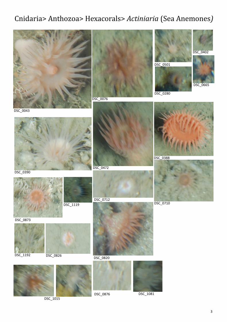
Cnidaria> Anthozoa> Hexacorals> Actiniaria (Sea Anemones)

DSC_0501

DSC_1015

DSC_0388

DSC_0390

DSC_0043

DSC_0076

DSC_0402

DSC_0472

DSC_0712 DSC_0710

DSC_0820

DSC_0665

DSC_0873

DSC_0876 DSC_1081

DSC_1119

DSC_0826 DSC_1192

4

Cnidaria> Anthozoa> Hexacorals> Zoantharia

DSC_0200 DSC_0321

DSC_0041 DSC_0082 DSC_0082 DSC_0233 DSC_0257 DSC_0302 DSC_0804

DSC_1193

DSC_0710

DSC_0124-11

5

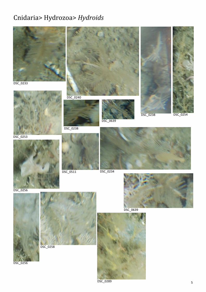
Cnidaria> Hydrozoa> Hydroids

DSC_0233

DSC_0234

DSC_0238

DSC_0238

DSC_0240

DSC_0253

DSC_0254

DSC_0256

DSC_0256

DSC_0258

DSC_0289

DSC_0511

DSC_0639

DSC_0639

6

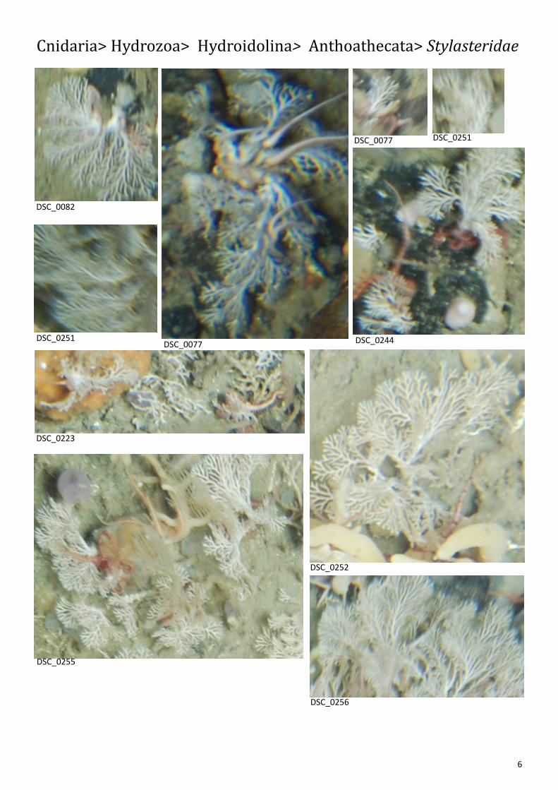
Cnidaria> Hydrozoa> Hydroidolina> Anthoathecata> Stylasteridae

DSC_0223

DSC_0244 DSC_0251 DSC_0077

DSC_0077

DSC_0082

DSC_0251

DSC_0252

DSC_0255

DSC_0256

7

Echinodermata> Asteroidea

DSC_0820-Echinasteridae

DSC_0043-Solasteridae

DSC_0078-Solasteridae

DSC_0224-Goniasteridae

DSC_0243-ilac-Asteriidae? °

DSC_0255-Pterasteridae?

DSC_0300-Echinasteridae

DSC_0385-Goniasteridae

DSC_0500-Echinasteridae

DSC_0593-Echniasteridae

DSC_0606-Echniasteridae

DSC_0620-Goniasteridae

DSC_0628-Echinasteridae

DSC_0708-Solasteridae

DSC_0708-Astropectinidae?

DSC_0921-Solasteridae?

DSC_1010-Ptreasteridae

DSC_1013-Pterasteridae

DSC_1016-Pterasteridae DSC_1017-purple

DSC_1230-Goniasteridae?

DSC_1233-Goniasteridae

8

DSC_0233

DSC_0108

DSC_0236

DSC_0236

Echinodermata> Ophiuroidea

DSC_0233

DSC_0233

DSC_0237

DSC_0251

DSC_0251

DSC_0251

DSC_0252

DSC_0273

DSC_0274

DSC_0275

DSC_0277

DSC_0276 DSC_0284

DSC_0285

DSC_0285

DSC_0046

9

DSC_0256

DSC_0893 DSC_1000

Echinodermata> Echinoidea

DSC_0242 DSC_0251 DSC_0275

DSC_0284

10

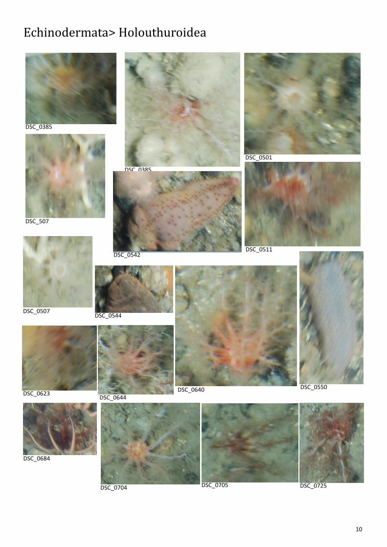
Echinodermata> Holouthuroidea

DSC_0385

DSC_0385

DSC_0501

DSC_507

DSC_0507

DSC_0511 DSC_0542

DSC_0544

DSC_0550 DSC_0623

DSC_0640 DSC_0644

DSC_0684

DSC_0704 DSC_0705 DSC_0725

11

DSC_0254

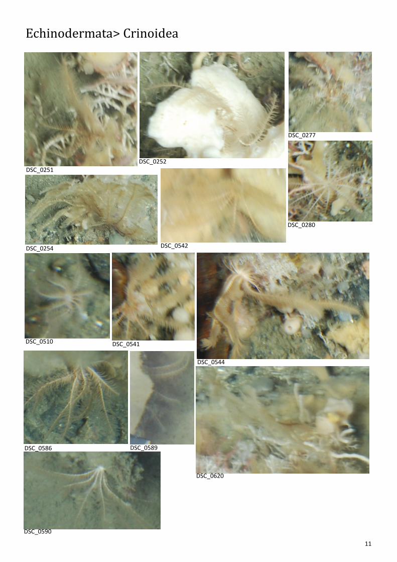
Echinodermata> Crinoidea

DSC_0251

DSC_0252

DSC_0277

DSC_0280

DSC_0510 DSC_0541

DSC_0542

DSC_0544

DSC_0586 DSC_0589

DSC_0590

DSC_0620

12

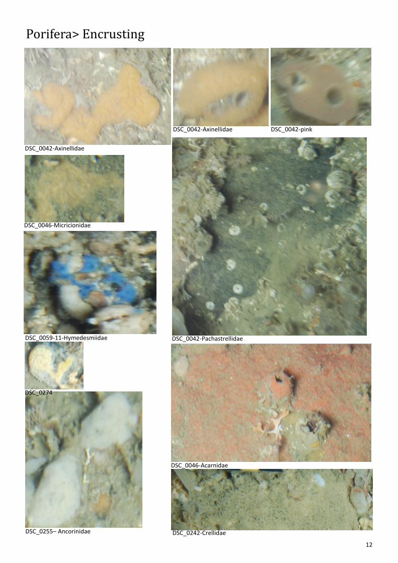
Porifera> Encrusting

DSC_0042-Axinellidae

DSC_0042-Axinellidae DSC_0042-pink

DSC_0042-Pachastrellidae

DSC_0046-Acarnidae

DSC_0242-Crellidae DSC_0255– Ancorinidae

DSC_0274

DSC_0046-Micricionidae

DSC_0059-11-Hymedesmiidae

13

Porifera> Massive

DSC_0107– Polymastiidae DSC_0267-Tethyidae DSC_0258-Polymastiidae

DSC_0041-Sycettidae DSC_0252-Grantiidae

DSC_0239-Polymastiidae

DSC_0239-Suberitidae

DSC_0390

DSC_0501

DSC_00628—Esperiopsidae

DSC_0644

DSC_0256-Aninellidae

DSC_0060-11– Grantiidae

14

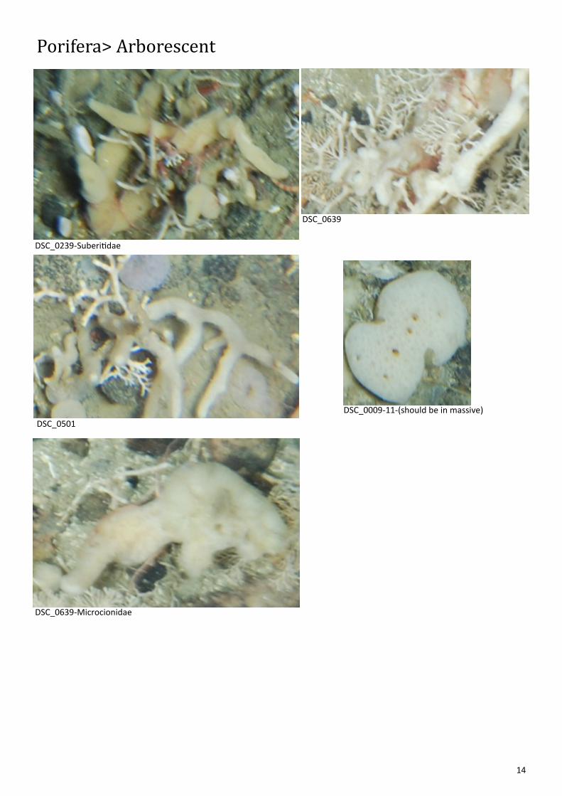
Porifera> Arborescent

DSC_0239-Suberitidae

DSC_0501

DSC_0639-Microcionidae

DSC_0639

DSC_0009-11-(should be in massive)

15

Annelida> Polychaetes

DSC_0077-Sabellidae

DSC_0644_Serpulidae

DSC_1123

DSC_0125-11-Polynoide

DSC_0059-11-Serpulidae

16

Arthropoda> Malacostraca> Eumalacostraca> Decapoda

DSC_0413-Majidae

DSC_0430-Majidae

DSC_0743-Paguroidea

DSC_1131

DSC_0862-Paguroidea

17

Arthropoda> Malacostraca> Eumalacostraca> Decapoda

DSC_0413

DSC_0040-shrimp?

DSC_0038-shrimp?

18

Arthropoda> Pycnogonida> Pantopoda

DSC_0221

DSC_0703

DSC_0804

DSC_0919

DSC_1071

DSC_1084

DSC_1092 DSC_1131

DSC_0125-11

19

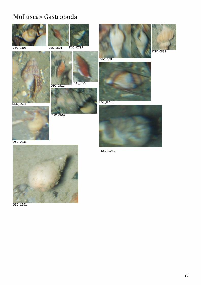
Mollusca> Gastropoda

DSC_0301 DSC_0501

DSC_0504

DSC_0511 DSC_0626

DSC_0667

DSC_0684

DSC_0733

DSC_0733

DSC_0799 DSC_0838

DSC_1071

DSC_1191

20

Mollusca> Chitons

DSC_0772

DSC_0618

DSC_0125-11

DSC_0130-11

21

Mollusca> Bivalves

DSC_0076

DSC_0077

DSC_0107

DSC_0107

DSC_0107

DSC_0218

DSC_0227

DSC_0507

DSC_0507

DSC_0510

DSC_0511 DSC_0592

DSC_0642

DSC_0642

DSC_0643

22

Mollusca> Scaphopoda

Mollusca> Cephalopods> Sepiida

DSC_0076

DSC_0078

DSC_0584 DSC_0584

DSC_0746

DSC_0776

23

Brachiopoda> Articulata> Terebratulida

DSC_0283

DSC_0387

DSC_0390

DSC_0390 DSC_0519

DSC_0592

DSC_0628

DSC_0643-?

DSC_0995

24

Bryozoa> Erect

DSC_0255

DSC_0040

DSC_0642 DSC_0642

DSC_0860

DSC_1255

DSC_1030

DSC_0862

25

Bryozoa> Encrusting

DSC_0743

DSC_0107

DSC_0669

DSC_0937

DSC_0937

26

Bryozoa> Soft

Chordata> Ascidiacea

DSC_0043

DSC_0043

DSC_0041 DSC_0822

DSC_0822

DSC_0822

DSC_0511

DSC_1214

DSC_0043-stalked-Polyclinidae

DSC_0038-Molgulidae

DSC_0078-Ascidiidae

DSC_1238-grey-Polycitoridae

DSC_0239-Styelidae

DSC_0125-11-Didemnidae

27

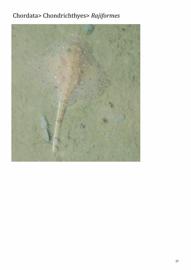
Chordata> Chondrichthyes> Rajiformes

28

Chordata> Osteichthyes> Scorpaeniformes

29

Chordata> Osteichthyes> Perciformes

DSC_0205

DSC_0418

DSC_0882

DSC_0892

DSC_0964

30

Chordata> Osteichthyes> Pleuronectiformes

DSC_0273

DSC_1073

DSC_1229

31

Dr Kirsty Kemp

Poppy Simon

Irina Chemshirova

42

Appendix 1.4

Table 3. Abundance of taxa in the two time periods

Taxa 1970s 1980s

Encrusting Bryozoa 379 404

Ascidians 330 209

Decapoda 152 146

Erect Bryozoa 116 184

Massive Sponges 95 97

Encrusting Sponges 75 113

Soft Bryozoa 74 117

Brittle stars 52 101

Arborescent Sponges 50 42

Sabellidae 43 10

Serpulidae 37 54

Anemones 34 37

Stylasterina 33 65

Unknown 30 53

Perciformes 13 19

Soft Coral 12 24

Terebratulida 7 3

Echinasteridae 5 4

Hydroids 5 8

Pleuronectiformes 5 6

Crinoids 3 0

Goniasteridae 3 5

Seacucumbers 3 3

Seaurchins 2 0

Starfish Other 2 3

Zoanthids 2 7

Astropectinidae 1 1

Bivalves 1 3

Gastropods 1 4

Isopoda 1 0

Polynoidae 1 0

Pterasteridae 1 0

Rajiformes 1 1

Amphipoda 0 0

Aphroditidae 0 0

Asteriidae 0 5

Chitons 0 0

Eunicidae 0 2

Octopoda 0 0

43

Scaphopods 0 1

Scorpaeniformes 0 1

Seaspiders 0 1

Appendix 1.5

Figure 1. Species accumulation curves for both time periods, blue is for the 1970s, green for the 1980s.

5 10 15

05

10

15

20

25

30

35

Sites

Ta

xa

44

Appendix 1.6

Table 4. Stations from both time periods paired based on their location, including the group number based on their location pairings

Stations 1970s

Stations 1980s

Station groups

5609 6713 1

5453 6715 2

5606 6716 3

5605 6717 4

5601 6720 5

5739 6721 6

5447 6722 7

5867 6724 8

5612 6727 9

5613 6728 10

5743 6729 11

5738 6730 12

5870 6731 13

5869 6732 14

5871 6733 15

5859 6736 16

5444 6737 17

5861 6738 18

5737 6749 19

45

Appendix 1.7

Table 5. The results of the Wilcoxon paired rank test between the 1970s and 1980s diversity metrics with the Class dataset

Diversity Index Result

Taxon Richness V=52.5, p=0.5

Number of Individuals V=85.5, p=0.7

Pileou’s Evenness V=105, p=0.7

Shannon Index V=95, p=1

46

Appendix 1.8

Figure 2. nMDS plot for the 1970s with taxonomic identification to Class level. Substrata 0.001 *** Stress = 0.12

-1.5 -1.0 -0.5 0.0 0.5 1.0

-1.5

-1.0

-0.5

0.0

0.5

1.0

1970s

NMDS1

NM

DS

2

5609

5453

5606

5605

5601

5739

5447

5867

5612

5613

5743

57385870

5869

5871

5859

5444

58615737

Substrata

soft

hard

-1.5 -1.0 -0.5 0.0 0.5 1.0

-1.0

-0.5

0.0

0.5

1.0

Species 1970s

NMDS1

unspecified

anthozoahydrozoa

asteroidea

ophiuroidea

echinoidea

holothuroidea

crinoidea

demospongiaepolychaeta

malacostraca

gastropoda

bivalvia

rhynchonellata

gymnolaematastenolaemata

ascidiacea

elasmobranchii

actinopterygii

NMDS1

NM

DS

2

X1

Y1

Depth1

Fishing.Log

Substrata1

Bioturbation1

47

Figure 3. nMDS plot for the 1980s with taxonomic identification to Class level. Substrata 0.003 *** Stress = 0.15

-1.0 -0.5 0.0 0.5 1.0 1.5

-1.0

-0.5

0.0

0.5

1.0

1980s

NMDS1

NM

DS

2

6713

6715

6716

6717

6720

6721

6722

6724

6727

6728

6729

6730

6731

67326733 6736

6737

6738

6749

Substrata

soft

hard

-1.0 -0.5 0.0 0.5 1.0 1.5

-0.5

0.0

0.5

1.0

1.5

Species 1980s

NMDS1

unspecified

anthozoa

hydrozoaasteroidea

ophiuroidea

holothuroidea

demospongiae

polychaeta

malacostraca

pycnogonida

gastropoda

bivalvia

scaphopoda

rhynchonellata

gymnolaemata

stenolaemata

ascidiacea

elasmobranchii

actinopterygii

NMDS1

NM

DS

2

X2

Y2

Depth2

Fishing.LogSubstrata2

Bioturbation2

48

Appendix 1.9

Figure 4. Dendogram of the hierarchical clustering of the dataset at Class level.

67

16

56

06

67

37

56

05

67

13

58

67

67

24

67

28

67

49

56

13

57

37

67

29

54

44

56

09

57

43

56

12

58

61

67

27

67

33

54

53

67

21

57

38

58

70

67

38

58

59

67

30

67

31

58

71

54

47

56

01

58

69

57

39

67

15

67

36

67

22

67

32

67

17

67

20

05

01

00

15

02

00

25

03

00

Cluster Dendrogram

hclust (*, "complete")

all.dist

He

igh

t

49

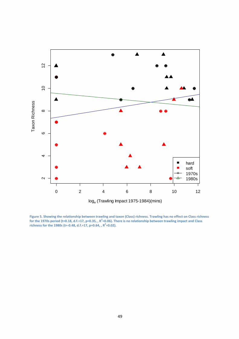
Figure 5. Showing the relationship between trawling and taxon (Class) richness. Trawling has no effect on Class richness for the 1970s period (t=0.18, d.f.=17, p=0.35, , R

2=0.06). There is no relationship between trawling impact and Class

richness for the 1980s (t=-0.48, d.f.=17, p=0.64, , R2=0.02).

0 2 4 6 8 10 12

24

68

10

12

loge (Trawling Impact 1975-1984)(mins)

Ta

xo

n R

ich

ne

ss

hard

soft

1970s

1980s

50

Appendix 2.1

Figure 6. Showing the relationship between β diversity and trawling impact. Increasing trawling impact had no effect on the β diversity observed at Class level (t=0.55, d.f.=17, p=0.59, R

2=0.017).

0 2 4 6 8 10

0.1

0.2

0.3

0.4

0.5

0.6

loge (Trawling Impact 1982-1984)(mins)

Be

ta D

ive

rsity

51

Appendix 2.2

Figure 7. Species accumulation curve for the 1984 dataset, further sampling will most likely not uncover new species.

0 5 10 15 20 25 30 35

01

02

03

04

0

Sites

Sp

ecie

s

52

Appendix 2.3

Figure 8. nMDS plot of the 1984 dataset. Substrata was the only environmental vector which explained the variation seen (p<0.01 **, Stress = 0.19)

-1.5 -1.0 -0.5 0.0 0.5 1.0

-1.5

-1.0

-0.5

0.0

0.5

1.0

Stations

NMDS1

NM

DS

2

Substrata

soft

hard

-1.0 -0.5 0.0 0.5 1.0

-1.0

-0.5

0.0

0.5

1.0

Species

NMDS1

unspecifiedsoftcoral

anemones

zoanthids

hydroids

stylasterina

asteriidae

pterasteridae

echinasteridae

solasteridae

goniasteridae

astropectinidae

starfishother

brittlestars

seaurchins

seacucumbers

crinoids

encrustingspmassivesp

arborescentspsabellidae

eunicidae

serpulidaem

decapoda

seaspidersgastropods

bivalves

scaphopods

sepioida

terebratulidaerectbr

encrustingbrsoftbr

ascidians

rajiformes

scorpaeniformes

perciformes

pleuronectiformes

NMDS1N

MD

S2

Substrata

Depth2

X

Y

Fishing.Log

53

Appendix 2.4

Figure 9. Linear regessions showing the relationship between trawling intensity and the following diversity indices: Taxon richness (t=-0.62, d.f.=34, p=0.54, R

2=0.011), Number of Individuals (t=-0.98, d.f.=34, p=0.33, R

2=0.027), Pielou’s

Evenness (t=0.84, d.f.=34, p=0.41, R2=0.020), Shannon Index (t=0.29, d.f.=34, p=0.77, R

2=0.002).

0 2 4 6 8 10 12

510

15

20

loge (Trawling Impact)(mins)

Specie

s R

ichness

0 2 4 6 8 10 12

34

56

loge (Trawling Impact)(mins)

log

e(N

o.

of

Indiv

iduals

)

0 2 4 6 8 10 12

0.4

0.5

0.6

0.7

0.8

0.9

loge (Trawling Impact)(mins)

Pie

lou's

Evenness

0 2 4 6 8 10 12

0.5

1.0

1.5

2.0

2.5

loge (Trawling Impact)(mins)

Shannon I

ndex

54

Appendix 2.5

Figure 10. nMDS plot of both time periods showing a clear separation of substrata (Stress = 0.16)

-1.0 -0.5 0.0 0.5 1.0 1.5

-1.0

-0.5

0.0

0.5

Overall

NMDS1

NM

DS

2

Substrata and Year

hard

soft

1970s

1980s