Benthic Macroinvertebrate Biological Monitoring Protocols ... · Benthic Macroinvertebrate...

Benthic MacroinvertebrateBiological Monitoring Protocols for

Rivers and Streams

2001 Revision

August 2001

Publication No. 01-03-028printed on recycled paper

This report is available on the Department of Ecology home page on theWorld Wide Web at http://www.ecy.wa.gov/biblio/0103028.html

For additional copies of this publication, please contact:

Department of Ecology Publications Distributions OfficeAddress: PO Box 47600, Olympia WA 98504-7600E-mail: [email protected]: (360) 407-7472

Refer to Publication Number 01-03-028

The Department of Ecology is an equal opportunity agency and does notdiscriminate on the basis of race, creed, color, disability, age, religion, nationalorigin, sex, marital status, disabled veteran's status, Vietnam era veteran's status,or sexual orientation.

If you have special accommodation needs or require this document in alternativeformat, please contact Michelle Ideker, Environmental Assessment Program, at(360)-407-6677 (voice). Ecology's telecommunications device for the deaf(TDD) number at Ecology Headquarters is (360) 407-6006.

Benthic MacroinvertebrateBiological Monitoring Protocols for

Rivers and Streams

2001 Revision

byRobert W. Plotnikoff

andChad Wiseman

Environmental Assessment ProgramOlympia, Washington 98504-7710

August 2001

Publication No. 01-03-028printed on recycled paper

Page i

Table of Contents Page

Introduction ......................................................................................................................... 1

Purpose of this Document ............................................................................................. 1

Background ................................................................................................................... 1

Objectives...................................................................................................................... 2

Program Organization ......................................................................................................... 3

Personnel ....................................................................................................................... 3

Experience..................................................................................................................... 3

Study Design ....................................................................................................................... 4

General Design.............................................................................................................. 4

Searching for a Regional Framework............................................................................ 5

Reference Conditions .................................................................................................... 5

Ecoregion Representation ............................................................................................. 6

Classification by Empirical Modeling........................................................................... 7Land Use Representation .............................................................................................. 8

Index Period .................................................................................................................. 9

Stream Size.................................................................................................................... 9

Habitat Type.................................................................................................................. 9

Field Quality Assurance .................................................................................................... 10

Sampling Precision...................................................................................................... 10

Representativeness ...................................................................................................... 10

Completeness .............................................................................................................. 10

Comparability.............................................................................................................. 11

Safety Procedures.............................................................................................................. 12

Field and Laboratory Preservatives............................................................................. 12

Miscellaneous.............................................................................................................. 12

Field Operations ................................................................................................................ 13

Landscape Attributes................................................................................................... 13

Reach Location............................................................................................................ 13

Macroinvertebrate Sample Locations.......................................................................... 13

Sampling Stream Macroinvertebrates ......................................................................... 14

Page ii

Habitat Survey Rationale ............................................................................................ 15

Surface Water Quality................................................................................................. 16

Stream Flow ................................................................................................................ 16

Stream Reach Profile................................................................................................... 17

Canopy Cover.............................................................................................................. 17

Substrate Characterization........................................................................................... 17

Human Influence ......................................................................................................... 18

Sequence for Conducting Field Operations ................................................................ 18

Laboratory Sample Processing.......................................................................................... 21

Benthic Macroinvertebrate Samples ........................................................................... 21

Benthic Macroinvertebrate Identification ................................................................... 21

Laboratory Quality Assurance .................................................................................... 22

Data Analysis .................................................................................................................... 23

Data Preparation.......................................................................................................... 23

Data Transformations (selecting the type of transformation) ..................................... 24

Criteria Development .................................................................................................. 24

Pattern Analysis- Ordinations ..................................................................................... 25

Pattern Analysis- Clustering........................................................................................ 26

Assessment of Classification Strength ........................................................................ 26

Data Management ............................................................................................................. 28

Literature Cited ................................................................................................................. 30

Appendices

A. Field Forms for Chemical and Physical Habitat Assessments

Page iii

List of FiguresPage

Figure 1. Washington State Ecoregions as defined by Omernik and Gallant (1986). ............7

Figure 2. Sequence of field operations..................................................................................19

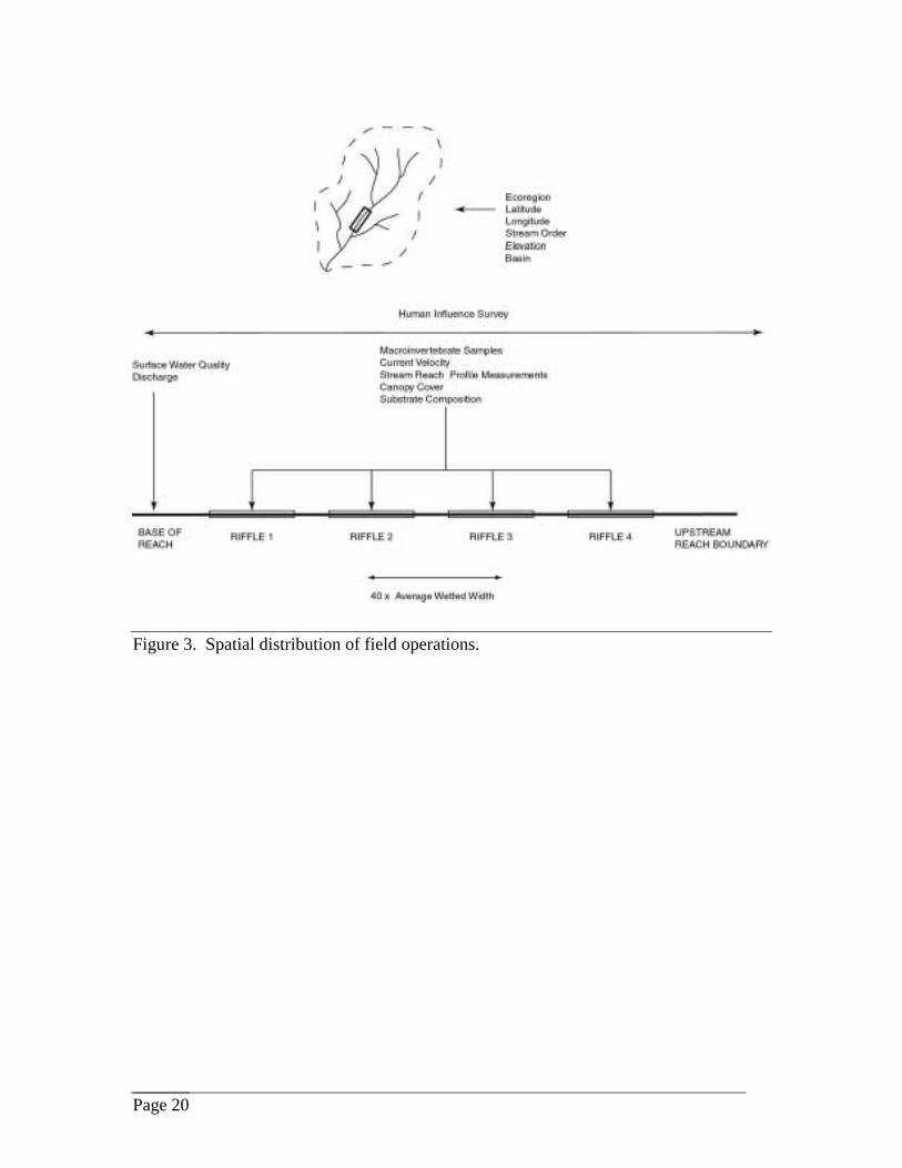
Figure 3. Spatial distribution of field operations...................................................................20

Figure 4. Database structure used by the Ecology Freshwater Ambient BiologicalAssessment Program..............................................................................................29

Page iv

Page v

Abstract

This document describes the Washington State Department of Ecology's Freshwater AmbientBiological Assessment Program. Outlined within the document are: 1) the sampling design, 2) thesite selection process, 3) field implementation, 4) laboratory processing of data, and 5) analysisand interpretation of data. The document also includes all of the elements necessary to serve as aQuality Assurance Project Plan (QAPP) for biological monitoring. Field operations remainconsistent with previous work (Plotnikoff 1992; 1994; 1998; 1999; Plotnikoff and Ehinger 1997).Relative to the original protocols document (Plotnikoff 1994), this revision provides additionaldetail for field operations, sub-sampling procedures, and data analysis procedures.

IntroductionPurpose of this DocumentThis document describes the Washington State Department of Ecology (Ecology)Freshwater Ambient Biological Assessment Program. Outlined here are:

♦ Sampling design.♦ Site selection process.♦ Field implementation.♦ Laboratory processing of data.♦ Analysis and interpretation of data collected by the program.

This document also includes all of the elements necessary to serve as a Quality AssuranceProject Plan (QAPP). Field operations remain consistent with previous protocols(Plotnikoff 1992; 1994; 1998; 1999; Plotnikoff and Ehinger 1997). Relative to theoriginal protocols document (Plotnikoff 1994), this revision provides additional detail forfield operations, sub-sampling procedures, and data analysis procedures.

BackgroundThe Federal Clean Water Act (Section 101) mandates the development of watermanagement programs that evaluate, restore, and maintain the chemical, physical, andbiological integrity of the nation’s waters (U.S. EPA 1990). Traditional measurements ofchemical and physical components for rivers and streams do not provide sufficientinformation to detect or resolve all surface water problems. Biological evaluation ofsurface waters provides a broader approach because degradation of sensitive ecosystemprocesses is more frequently identified. Biological assessments supplement chemicalevaluation by:

♦ Directly measuring the most sensitive resources at risk.♦ Measuring a stream component that integrates and reflects human influence over

time.♦ Providing a diagnostic tool that synthesizes chemical, physical, and biological

perturbations (Hayslip 1993).

Ecology collects biological information from rivers and streams throughout the state.The long-term monitoring program was established in 1993 to explore spatial patternsand identify temporal trends in benthic macroinvertebrate communities. Gradually, theprogram has developed a large base of information that describes biologicalcharacteristics of reference and degraded conditions. Reference conditions are found instreams with little or no human impact.

This program is focused on determining methods for reliably interpreting biological andassociated habitat data. This is accomplished by delineating regions of relativelyhomogenous natural biological communities in the state and comparing streams withineach region along a gradient of impairment. Application of biological expectations arealso applied to broad geographic areas defined by existing regional descriptors and bylandscape variables such as elevation, climate zones, or topography. Identification offactors in streams that are directly correlated with biological attributes can be useful intracing the sources of impacts. Tools for interpreting data are developed by using knownstream conditions (naturally and highly degraded) and calibrating the responses of eachbiometric or community diversity measure to the known condition.

Biological information is used to evaluate stream impacts from point- and non-pointsources of pollution. Integrating this information with physical and chemicalcharacterization of a stream segment provides an effective way for diagnosing sources ofdegradation. The following discussion outlines the program under development foreffectively using biological information in environmental management.

ObjectivesLong-term biological monitoring of rivers and streams in Washington attempts toincorporate biological and associated habitat information into the regulation andconservation of environmental resources. Past and current development of biologicalcriteria to detect human-induced impacts in streams is an essential step in this process.Evaluation of biological criteria follows the acquisition of new information, which iscollected on an annual basis. Therefore, the objectives and applications of informationfrom this monitoring program are as follows:

♦ Verify regional stream classification scheme previously defined by physico-chemicaland species data.♦ Test existing physico-chemical dichotomous key stream classification♦ Test existing regional stream class indicator species lists and develop new

regional lists.♦ Develop criteria to evaluate human-induced disturbance in biological communities on

a regional basis.♦ Examine where and how biological information should be applied in water resource

management.

Program OrganizationPersonnelField operations are completed with three personnel who gather samples and measureenvironmental variables at each site. The senior scientist or project leader designs anddirects the components of the biological assessment program. A junior scientist orenvironmental technician collects biological and environmental data from rivers andstreams, performs laboratory sample sorting and taxonomic identifications, and recordsdata in a database.

ExperienceThe senior scientist must be able to: 1) independently design a project and direct fieldwork, 2) identify benthic macroinvertebrate taxa to the lowest practical taxon (e.g.Plotnikoff and White (1996)) with available taxonomic literature, 3) understand andapply current stream ecology theory for interpretation of the biological data, 4) operate avariety of computer software including word processors, spreadsheets, statisticalprograms, and databases, and 5) supervise junior personnel.

The junior scientist/environmental technician must be able to: 1) understand projectdesign and implement the components, 2) identify most taxa to family efficiently, 3) havea general knowledge of computer software operation, and 4) operate stream samplingequipment for measuring biological communities and physical variables.

Study Design

General DesignThis program uses representative riffle-habitat (broken surface water) sampling ofbenthic macroinvertebrates, physical habitat, and water quality to describe biologicalcommunity condition as a result of natural and human-induced disturbance. Normally,samples are collected from riffles to characterize the benthic macroinvertebratecommunity unless degradation is suspected in pool habitat (slow moving or eddyingwater). To distinguish natural versus human influence, data must be collected atreference sites and at degraded sites over a period of time to address spatial and temporalvariability.

Reference sites are intended to represent relatively unimpacted or least impactedconditions. Minimally disturbed conditions reflect sites that have experienced very littlehistorical activity that alters stream integrity. Least disturbed sites have been degradedhistorically, but exhibit some level of recovery. Reference sites are used to describebiological variability due to natural disturbances (e.g. precipitation, drought).

Degraded sites are surveyed to describe a continuum of human influence on naturalstream communities. Identification of what a degraded macroinvertebrate community isand the factor(s) that caused the resulting condition defines severity of impact. Thisgradient of biological condition is used to determine the levels of human-induceddisturbance that are excessive in a waterbody.

Long-term biological monitoring in this program has been conducted since 1993 andincorporated a variety of site conditions. Besides high-quality reference conditions, siteswith high levels of physical and chemical modifications have been surveyed. The resultis a data set that represents a gradient of biological conditions as a response to theexisting stream condition.

The biological community in rivers and streams represents an important source ofinformation when evaluating ecological integrity. We use a single biological component,the benthic macroinvertebrates, to evaluate stream condition. Evaluation of the fishcommunity is not used as a sole source of information because of species paucity inwestern North America (Moyle et al. 1986) and continuing harvest restrictions on severalsalmon species.

Searching for a Regional FrameworkDefining the distribution of aquatic invertebrate species is an important exercise inknowing how to use biological information as a guide for resource management. Thesearch for spatial pattern in biological communities serves to describe minimumexpectations in stream types across the state especially when a subset of streams issurveyed. A large base of biological information is usually required before communitypatterns emerge from analysis of the data, especially when the landscape has variableclimatic topographic features.

In Washington State streams, distinct regional patterns exist among the benthicmacroinvertebrate communities. Variables at different spatial scales are often required toexplain regional patterns in benthic macroinvertebrate communities (Hawkins et al.2000). Plotnikoff (1992) found that communities differ as a function of region andseason among similar-sized streams in three ecoregions (Puget Lowland, CascadeMountains, and Columbia Basin). Surveys in the Yakima River Basin, Washingtonidentified segment-level variables (valley type and watershed characteristics) as the bestcorrelates with biological community expressions over basins and regions of thelandscape (Carter et al. 1996). Plotnikoff and Ehinger (1997) stressed the importance ofreach-level variables (temperature, pH, conductivity, wetted width/ bankfull width ratio,elevation) in shaping the macroinvertebrate communities. The large-scale expressionssuch as ecoregions (Omernik and Gallant 1986; Pater et al. 1998) or components ofecoregion descriptions like topography, elevation, or climate can be helpful in parsingstreams into groups. These divisions are important for describing biological expectationsin stream classes and are consistent with how criteria are applied in most regulatoryagencies. Smaller-scale variables, however, are needed in order to explain additionalnatural variability and increase the likelihood of identifying human-induced changes instream communities.

Reference ConditionsThe reference condition is the physical, chemical, and biological condition of a class ofstreams with little or no human-induced degradation. High road densities and thepresence of other human activities in Washington State necessitate the use of a minimallydisturbed or least disturbed definition for reference. Minimally disturbed conditionsreflect sites that have experienced very little historical activity that alters stream integrity.Least disturbed sites have been degraded historically, but exhibit some level of recovery.

Reference site information is used as a measure of biological potential for particularstream settings. Identifying a response in the biological community to environmentaldegradation is determined by comparison to a reference site. For consistency in amonitoring program, identification of reference sites should follow these guidelines:

♦ Map potential areas where reference sites are expected.

♦ Evaluate whether candidate reference areas are concentrated in one part of awatershed or are in a variety of locations (candidate sites may not be physicallycomparable to degraded sites if they are unique to a small portion of a watershed).

♦ Eliminate areas with relatively high human modifications (past and present).♦ Field visits; verify current condition of each site.♦ Choose reference sites that approximate stream type and setting as those that will be

surveyed for suspected degradation.

Evaluation of regional patterns and variability is most effective in the absence of anyhuman degradation. Degraded sites may introduce error into observed regional patterns,unless there are intrinsic biological attributes within a stream class that persist over adegradation gradient. If all streams in the region have been disturbed to a certain degree,however, a least disturbed condition must be identified and used for that region. Wesuspect this situation to arise in the Columbia Basin.

Ecoregion RepresentationEcoregions are geographical regions of relative homogeneity either in ecological systemsor involving relationships between organisms and their environment (Omernik andGallant 1986; Pater et al. 1998). Surficial, climactic, and hydrological characteristics areused to define these regions of relative homogeneity. These characteristics include landsurface form, potential natural vegetation, land use, soils, mean annual precipitation, andmean temperature. The Freshwater Ambient Biological Assessment Program currentlyuses ecoregions as an a priori stream classification approach.

Information from sample sites is extrapolated to other similar streams within anecoregion framework. It is, therefore, important to represent the variety of streamconditions within ecoregions to interpret results generated by this program. Regionalbiological description is defined by including information from a variety of referencesites within the ecoregion.

Washington State is comprised of eight ecoregions: Coast Range, Puget Lowland,Cascades, Columbia Basin, Northern Rockies, Willamette Valley, Blue Mountains, andEastern Cascade Slopes and Foothills (Figure 1). Biological condition is describedwithin-regions and inter-annually over five year periods in order to quantify naturalvariability. Analysis of data within regions describes the range of biological communityconditions expected spatially. Measuring inter-annual variability identifies the influenceof cyclic environmental phenomena (e.g. annual precipitation patterns, ambient airtemperature) on biological communities. A few long-term benthic monitoring sites areused as a calibration tool that measures inter-annual variability. New reference sites aresampled periodically in each ecoregion in order to test and refine regional referencecondition.

Figure 1. Washington State Ecoregions as defined by Omernik and Gallant (1986).

Classification by Empirical ModelingMany studies have suggested that large-scale regionalizations, such as ecoregions, do notaccount for an acceptable amount of natural variability (See Hawkins et al. (2000) for asynthesis). One alternative is to use large-scale regionalizations as an initial stratificationvariable, and then use smaller scale variables to account for more of the naturalvariability. Modeling reference streams along environmental gradients at large and smallspatial scales can accomplish this. The first step is to construct biological classes fromthe biological similarity of reference streams throughout the state. Stream communitiescan be clustered into biological classes with multivaritiate classification tools.Multivariate classification clusters sites in such a way that within-class variability isminimized relative to between-class similarity (i.e. those that are most similar to eachother). Reference conditions defined by a posteriori clustering differs from a prioriregionalizations because the biology is used to delineate natural breaks in biologicalreference condition. When biological classes are identified, regional and reach-scaleenvironmental variables from the same reference sites are used to construct models foreach biological class. The same environmental variables from the independent test sitescan then be applied to the empirical models to ascertain biological class membership.Biological class membership is defined in terms of probabilities, so a test site maybelong, in part, to many biological classes (Moss et al. 1987).

Land Use RepresentationStream sample sites that have a gradient of land-use influences are chosen annually formonitoring in at least two ecoregions. The type of land use within an ecoregioninfluences biological communities and these relationships are described with independentstream surveys. Dominant land use within priority basins and ecoregions is initiallydetermined. A visual estimate of the severity of land use is made to ensure that sites arechosen to represent a gradient of human influence. Visual estimates are based on mapsand ortho-photos, followed by ground truthing in the watershed. This hypotheticalimpact gradient is further validated when field information is analyzed as described in asubsequent section of this document. Sampling and analysis of degraded stream reacheshas a two-fold purpose:

♦ Validate acceptable reference condition delineation.♦ To determine the sensitivity of biological information in detecting impacts.

The land use coverage that has been used was Anderson et al. (1976). Current land usecoverages, such as those found at http://www.epa.gov/mrlc/nlcd.html andhttp://www.epa.gov/OST/BASINS/ are being used in the program. The following listdetails the land uses represented in past analyses:

ResidentialCommercial and ServicesIndustrialTransportation, Communications,UtilitiesMixed Urban or Built-Up LandOther Urban LandAgriculturalCropland and PastureOrchards, Groves, Vineyards, andNurseriesConfined Feeding OperationsOther Agricultural LandHerbaceous RangelendShrub and Brush RangelandMixed RangelandDeciduous Forest LandEvergreen Forest LandMixed Forest LandLakesReservoirsBays and EstuariesForested WetlandNonforested WetlandBeaches

Sandy Areas Other Than BeachesBare Exposed RockStrip Mines, Quarries, and Gravel PitsTransitional AreasMixed Barren LandShrub and Brush TundraHerbaceous TundraBare Ground TundraWet TundraMixed TundraPerennial SnowfieldsGlacier

Index PeriodThe index period is a time span during the year in which samples are collected. Theindex period used in this program (July 1st -October 15th) was chosen for the followingreasons:

♦ Adequate time is available for the instream environment to stabilize following naturaldisturbances (e.g. spring floods).

♦ Many macroinvertebrates reach body sizes that can be readily identified.♦ Representation of benthic macroinvertebrate species reaches a maximum, particularly

during periods of pre-emergence (typically mid-spring to late-summer).

Biological assessments can yield different interpretations depending on the index periodchosen. This is because natural seasonal disturbances and physical stream conditionsstrongly affect the diversity, abundance, and life stage progression of aquatic insects(Hynes, 1970; Vannote et al. 1980). It is recommended that collecting begins earlier inthe index period for drier ecoregions and that all sites within an ecoregion are visitedduring an abbreviated period of time.

Stream SizeWe sample streams that are perennial and wadeable. Seasonal drought disturbanceselects for distinct specialist communities (Resh et. al. 1988; Clifford 1966). Stochasticdrought is a catastrophic natural disturbance that eliminates many taxa (Resh 1982; Reshet. al. 1988). These natural disturbances introduce natural variability into the data set,making community pattern identification difficult. Unwadeable streams present logisticalproblems and require different macroinvertebrate sampling techniques that are beyondthe scope of this protocol.

Habitat TypeStream reaches contain two easily identified and contrasting habitats: riffles (brokensurface water) and pools (slow-moving or eddying water). The primary reason forsurveying these two habitats is to measure habitat-specific signals from stressedinvertebrate communities. Degradation may selectively occur in pool habitat and not inriffles. Comparison of pool invertebrate assemblages to riffle invertebrate assemblagesmay reveal the effect of natural hydrologic disturbance, as well as the biological responseresulting from physical disturbance (Minshall and Minshall 1977; Brown and Brussock1991). From 1993- 1996, Ecology’s Freshwater Ambient Biological AssessmentProgram sampled both riffle and pool habitat. Even though degradation may selectivelyoccur in pool habitat and not in riffles, no consistent biological differences (due todegradation) between riffles and pools were detected in this survey (Plotnikoff andEhinger 1997). As a result, we have placed exclusive regular monitoring effort insampling riffles following work completed in 1997. Pools are sampled when degradationis suspected in that habitat.

Field Quality AssuranceSampling and Visit PrecisionSampling precision is related to the variability of the four riffle samples that arecomposited. Sampling precision is estimated by keeping the four replicate riffle samplesseparate at 10% of the reaches sampled annually. Pool habitat is not examined forsampling precision estimates. Sampling precision is calculated using the coefficient ofvariation (CV) from four replicate riffle samples and should be ≤ 20% in referencestreams when using the taxa richness metric (Plotnikoff, 1992). We expect collections ofmacroinvertebrates from multiple sample locations to have similar community structurein reference stream riffles.

Visit precision is related to the variability of collecting a composite sample in a reach.Visit precision is estimated by collecting three composite riffle samples within the samereach during the same day at 10% of the reaches sampled annually. Pool habitat is notexamined for visit precision estimates. Visit precision is calculated using the coefficientof variation (CV) from three replicate composite samples and should be ≤ 20% inreference streams when using the taxa richness metric.

RepresentativenessRepresentativeness of benthic community conditions is determined by the sampleprogram design (Lazorchak and Klemm, undated). The sampling protocol is designed toproduce consistent and repeatable results in each stream reach. Physical variabilitywithin riffles is accounted for through stratified sampling based on depth, substratedistribution, and location within the sample reach.

CompletenessCompleteness is defined as the proportion of useable data gathered (Kirchmer andLombard 2001). Sample loss is minimized with sturdy sample storage vessels andadequate labeling of each vessel. Sample vessel type and labeling information aredescribed under "Sampling Stream Macroinvertebrates." Sample contamination occurswhen containers are improperly sealed or stored. Loss of benthic material or desiccationdiminishes the integrity of the sample. If the validity of the information from the sampleis in question, the sample is excluded from analysis. The goal for completeness ofbenthic macroinvertebrate data sets is 95% of the total samples collected. Completenessis defined as the total number of samples that we are confident in using for further dataanalysis following field collection.

Sampler and operator efficiency both influence completeness. One measure ofsampler/operator efficiency is the number of taxa collected or "total taxa richness." Thediscrepancy between transects in the total number of taxa collected is attributed tosampler/operator efficiency (i.e. the ease with which various species can be collected)

and the distributional characteristics of benthic dwelling organisms. Some species areconsidered rare and may be difficult to collect due to low abundance or are difficult tosample in certain habitats.

ComparabilityComparability describes the confidence in comparing one data set to another. Manyprivate, academic, and governmental entities are currently generating biologicalinformation for rivers and streams that could potentially be incorporated into a larger dataset. Comparability of data sets is primarily achieved through adherence to commonlyaccepted protocols (e.g. field sampling, analytical methods and objectives). Ourmultihabitat collection approach using a D-frame kicknet was chosen largely to providenecessary comparability with other programs. These programs include the OregonDepartment of Environmental Quality's bioassessment program, the EnvironmentalProtection Agency's "Regional Environmental Monitoring and Assessment Program"(R-EMAP), and a reference site monitoring program that developed probability modelsbased on biodiversity in Washington streams (Hawkins and Ostermiller, PersonalCommunication).

Safety ProceduresField and Laboratory PreservativesBiological samples are preserved immediately following collection and consolidation intocontainers. Inadequate preservation often results in: 1) loss of prey organisms throughconsumption by predators, 2) eventual deterioration of the macroinvertebrate specimens,and 3) deformation of macroinvertebrate tissue and body structures making taxonomicidentification difficult or impossible.

The field preservative used in this program is 85% non-denatured ethanol. Thepreservative is prepared from a stock standard of 95% non-denatured ethanol.Flammability, health risks, and containment information are listed on warning labelssupplied with the preservative container. Detailed information can be found with the"Materials Safety Data Sheets" (MSDS) maintained by the Environmental AssessmentProgram Manager's Secretary. Minimal contact with the 95% non-denatured ethanolsolution is recommended.

The preservative used in handling sorted laboratory samples is 95% ethanol (non-denatured). Seventy-percent non-denatured ethanol is used for preservation of voucherspecimens in two dram vials (8 mL). Voucher specimens are stored in a flammablesstorage case in the Ecology Benthic laboratory. Bulk ethanol is stored in a separateflammables storage building. Hazard Communication Training is provided to allpersonnel that come into contact with hazardous materials while conducting programduties.

MiscellaneousField activities are conducted by at least two people. A contact person is designated atthe headquarters office to which field personnel report daily at pre-designated times.

Careful planning of field activities is essential and permission to access private land mustbe obtained. Access to private land is usually obtained through verbal agreement withthe landowner while at the proposed sample site.

Special safety equipment includes:

♦ Felt Soles or Cleats (for waders)♦ Rain Gear♦ Insulated Rubber or Neoprene Gloves♦ First Aid Kit (stored in the vehicle)♦ Department of Ecology Photographic Identification Card♦ Certification in CPR/First Aid♦ Defensive Driving Training

Field OperationsThe sequence and spatial arrangement of field operations are outlined in two figurestoward the end of this section. Companion pictures to the following field operations(page 18) can be found athttp://www.ecy.wa.gov/programs/eap/fw_benth/fwb_photos.html.

Landscape AttributesLandscape attributes are often important correlates with macroinvertebrate communitycomposition. The ecoregion, Strahler stream order (1:100,000 scale map), and basin arenoted for each site. These attributes are often recorded from maps prior to sampling.Latitude, longitude, and elevation are recorded in the field with a GPS unit. Accuracy ofthese measurements is verified in the office by comparing against digital maps of streamlocations in the state.

Reach LocationAt each site, the stream reach location is determined by identifying the lower end of thestudy unit and estimating an upstream distance of 40 times the average wetted streamwidth. The lower end of a study unit is located to represent a given land use. The streamreach length should measure approximately 150 meters if stream width is narrow (< 3meters). This reach length ensures that characteristic riffle/pool sequences arerepresented and potentially sampled.

Macroinvertebrate Sample LocationsFour biological samples are collected from riffle habitat in a reach. One sample iscollected from each of four riffle habitats. A variety of riffle habitats are chosen withinthe reach to ensure representativeness of the biological community. The locations withina reach are determined by finding representative combinations of the following variables:

♦ Depth of riffle.♦ Substrate size.♦ Location within a riffle area of the stream (forward, middle, back).

Sampling among several riffles in a stream increases representation of physicaldifferences in this habitat. Also, this sampling design maximizes the chance of collectinga larger number of benthic macroinvertebrate taxa from a reach than from fewer riffles.Variations in physical condition of the riffle habitat provide an opportunity to collect bothcommon and rare taxa.

When sampling pool habitat, benthic macroinvertebrates are collected at four locations.Each sample is collected from its own respective pool. The locations within a reach aredetermined by finding representative combinations of the following variables:

♦ Depth of pool.♦ Location within the channel (side, middle, behind a boulder/woody debris).

Absence of flowing water in pool habitat can result in low sampler efficiency. Moststream bottom samplers rely on flowing water to direct macroinvertebrates into acollection net. In the absence of flowing water, loss of individual organisms increases.Benthic organisms collected from pools provide reliable synoptic lists of taxa, but notcommunity characterizations calculated with density estimates.

Sampling Stream MacroinvertebratesMacroinvertebrate samples are collected from riffle and pool habitats with a D-Framekicknet (500-micrometer net mesh). A device fastened to the base of the D-Framekicknet encloses a one-foot by two-foot area in front of the sampler (sampling area= 0.19m2). In riffle samples, coarse substrate in the enclosed area is removed and scrubbedwith a brush to dislodge clinging invertebrates into the collection net. After scrubbingcoarse substrate, all remaining substrate in the enclosed area is agitated to a depth of 15cm for two minutes. Samples are stored in ethanol-filled containers.

Pool samples are more difficult to collect. Benthic-dwelling animals may escape in theabsence of a steady current. The D-frame kicknet is placed on the stream bottom and a 1foot x 2 foot area upstream of the collection net is disturbed by kicking. Stream bottommaterial will be suspended in the water column, particularly the organic material, and isactively “scooped” up with the collection net. Scooping requires the removal of the netfrom the stream bottom and collecting as much as possible from the water column. Thenet should follow a path of 1 x 2 feet through the water column when collecting thesuspended material. Disturbance of the substrate and scooping with the net is doneseveral times to ensure collection of most material in the pool collection area. Collectionat each pool location within a reach is continued for a period of two minutes.

Macroinvertebrate samples from most sites are composited into single riffle and poolsamples. As part of our data quality objectives, approximately 10 percent of total sitesmonitored in a year are included as part of an evaluation of community variability withina stream reach. Riffle samples are stored in separate containers as replicates at each ofthese streams. In projects that require a small-scale quantitative approach (e.g. upstream-downstream), the 0.19 m2 samples are always kept separate as replicates.

The macroinvertebrate field samples are preserved in 85% ethanol. Storage containerscan be either heavy-duty freezer bags or one-liter polycarbonate containers. A doublebag system is used when storing samples in freezer bags. Sample labels are placed in thedry space between the inner- and outer freezer bags. Label information should contain:name of stream (including reach identification), date of collection, County and State,project name (if applicable), type of habitat (e.g. riffle 1, riffle 2, …, riffle composite),and collector's name. Sample containers are assigned an identification number whenstored in the laboratory. Additional physical and chemical stream information isassociated with the numbered biological collections in the database.

Habitat Survey RationaleThe environmental characteristics of instream and riparian areas of streams have asubstantial influence on the structure and function of benthic macroinvertebratecommunities. Environmental characterization is used concomitantly with biologicalassessment surveys to: 1) understand the natural physical and chemical constraintsimposed on macroinvertebrate communities, and 2) detect physical and chemical changeswithin sensitive stream areas and adjacent riparian zones.

Environmental variables used in this monitoring program are listed below:

Surface Water Quality♦ temperature♦ pH♦ conductivity♦ dissolved oxygen

Stream Flow♦ discharge at base of reach♦ average current velocity♦ bottom current velocity

Stream Reach Profile♦ maximum depth♦ wetted width♦ residual pool depth♦ bankfull width♦ stream gradient

Canopy Cover♦ center-of-stream readings♦ left bank/right bank readings

Substrate Characterization♦ substrate composition (general description)

Human Influence♦ type of activity♦ proximity to the stream

Macroinvertebrate communities are affected by environmental variables on a number ofspatial scales. In addition to landscape features, environmental variables in the samplereach are measured at the “reach” and “sample” scale. Figure 3 illustrates where eachvariable is sampled in the sampling reach. The field forms used to record measurementsat each stream are in Appendix A.

Surface Water QualitySurface water analysis is limited to temperature, pH, dissolved oxygen, and conductivity.These variables are routinely measured in most of Ecology’s projects. Additionalobservations include water clarity, water/sediment odors, and surface films.Measurements of all surface water variables are made before biological samples arecollected.

Water samples are collected directly from the lowest portion of the sample reach andtransported back to the vehicle for measurement as quickly as possible. The followinginstruments and methods are used to measure surface water values:

Parameter Method Sensitivity

Temperature YSI Thermistor ± 0.1°Centigrade

pH Orion, Model 250A ± 0.1 pH Units

Conductivity YSI Conductivity Meter, ± 2.5 µmhos/cmNull Indicator @ 25°C

Dissolved Oxygen YSI Membrane Electrode, ± 0.2 mg/LModel 57or Winkler Titration ± 0.1 mg/L

Quality Assurance

Replicate water quality measurements are made for one of five sample sites visited. Biasis determined by comparing instrument readings with solutions of known concentration(e.g. buffers for pH, conductivity standard, and calibration of the thermometer).Comparability is assured by using standard procedures.

Stream FlowStream discharge is measured with a Marsh-McBirney flow meter and a top-set wadingrod. A stream cross-section at the bottom of the sampling reach is constructedperpendicular to the direction of flow. Velocities and depths are measured in cells acrossthe distance of the cross-section. The cross-section is divided into at least 20 cells,following the U.S. Geological Survey (USGS) Mid-section method for instream flowmeasurements (United States Bureau of Reclamation, 1997). Total discharge is thesummation of discharge in each cell. Discharge measured in each cell should not exceedten percent of the overall discharge estimate.

Average water column current velocity (0.6 x depth from water surface) and bottomcurrent velocity is measured at each macroinvertebrate collection site. Thesemeasurements provide information about the instream hydraulic conditions that biotaexperience.

Stream Reach ProfileA series of channel morphology features is measured at each macroinvertebrate samplesite. A transect perpendicular to stream flow at each macroinvertebrate sample site isidentified. Wetted width, bankfull width, and maximum depth is measured along eachtransect. The residual pool depth is measured in pool locations. The residual pool depthis the maximum pool depth minus the depth of the pool at the crest or “tailout”. Streamgradient is measured with a clinometer and reflects the local gradient of riffles wheremacroinvertebrates are collected.

Canopy CoverPercent canopy cover is estimated with multiple densiometer readings along eachmacroinvertebrate sample transect. Four readings are taken at the sample point (facingupstream, facing downstream, facing the right bank, and facing the left bank). Inaddition, one reading is taken facing the bank at the wetted right bank and left bank,respectively. Each measurement is taken one foot above the water surface. Thecomposite value is the sum of the four readings taken from the macroinvertebrate samplelocation.

Substrate CharacterizationFirst, substrate is characterized at each macroinvertebrate sampling location. A metalgrid with 50 equidistant points is placed on each macroinvertebrate sampling location.The substrate grid is an octagon with 21-inch dimensions from end to end. There are 50points arranged 3 inches apart from each other on the grid. The substrate size at eachpoint is categorized with a viewing tube. The viewing tube is a PVC tube with aPlexiglas bottom. The tube is 9 inches in diameter and twelve inches deep. Substrateclasses are located on the field form in appendix A. This field exercise normally requirestwo personnel. The first person: 1) keeps the grid stationary, 2) moves the viewing tubefrom point to point, and 3) calls off the substrate class at each point. The second personsimply records the information on the field sheet as tick marks. Four measurements (50values per measurement) are taken during each visit at each macroinvertebrate samplinglocation. Representation of each substrate class is calculated by multiplying a substrateclass tally by 2 and expressing as a percent. The measurements are taken beforemacroinvertebrate sampling occurs. Care is taken to avoid disturbing the substrate. Inthe deeper locations, disturbance is avoided by suspending the grid up above thesubstrate. In exceedingly shallow locations, adjacent substrate that is similar to thesampling location is used for substrate characterization.

An optional pebble count may be employed along each riffle cross-section contiguouswith each macroinvertebrate sampling location to characterize substrate at the reach scale(Wolman 1954; Harrelson et al. 1994; Schuett-Hames et al. 1999). One Hundredsubstrate particles are collected and measured along each cross-section. Data collectionstarts at a randomly selected point at one of the bankfull elevations along the cross-section. With an averted gaze, the sampler picks up the first particle touched by the tip ofthe index finger at the toe of the wader (Harrelson et al. 1994). The particle is measuredalong its b-axis. A substrate particle is 3-dimensional, with a long side, a short side, andan intermediate side. The b-axis is the intermediate dimension that determines if theparticle would pass through a sieve of that size. The sampler then steps in the directionof the opposite bank, picking up and measuring another substrate particle. The procedureis repeated until 100 measurements are made. The measurements are assigned to theproper size class and tallied. Size fractions are located on the field form in appendix A

The Wolman pebble-count has been used to characterize substrate composition along a“reach”. This method has been adopted for “site-specific” evaluations in this protocol.

Human InfluenceReach-scale human influence observations can be important for understanding biologicaland environmental information. Evidence of different types of human influence is notedin each sample reach. In addition, the proximity of each influence to the stream bank isvisually estimated.

Sequence for Conducting Field OperationsField procedures follow a sequence of measurements that ensure quality information iscollected and a reasonable amount of time is spent at each site. The sequence and spatialarrangement of field operations is outlined in figures 2 and 3, respectively. The seniorscientist selects sampling reaches prior to field work. The field crew consists of a leadand two assistants. Every person in the crew is qualified as at least a junior scientist, orunder direct supervision of a junior scientist. One field crew lead and two assistantsconduct biological monitoring. First, the two assistants collect surface water anddischarge information at the furthest downstream portion of the sample reach. Aftersurface water is collected for water quality measurements, the field crew lead selectsmacroinvertebrate sampling locations in different riffles. Sediment characterization andthe macroinvertebrate collection ensues. The field crew lead identifies themacroinvertebrate sampling locations with numbered flags. The two assistants followbehind the lead and collect current velocity, stream reach profile measurements, andcanopy cover at the sampling locations. One assistant alternates between the lead and theother assistant to help with different collection procedures. After macroinvertebrates arecollected from all four sampling locations, they are deposited into a container andpreserved with 85% ethanol. Evaluating human influence is the last component of a sitevisit. With this sampling sequence, stream disturbance is minimized before surface waterand biological information is collected.

Figure 2. Sequence of field operations.

Figure 3. Spatial distribution of field operations.

Laboratory Sample ProcessingBenthic Macroinvertebrate SamplesThe riffle samples collected at each site are sub-sampled using a 500-organism count.Macroinvertebrates are removed from a minimum of two randomly chosen squares in asub-sampling grid containing 30 squares. The dimension of each square is 6 cm x 6 cmand the tray has an overall dimension of 30 cm x 36 cm. The sample material from afield container is spread evenly on the base of the grid tray. We assume that theprocedure is random and unbiased. All organisms are removed from randomly chosensquares until a minimum of 500 macroinvertebrates are picked and the process iscontinued to include all remaining organisms in the selected squares. Largermacroinvertebrates are removed from the sample square prior to use of a dissectingscope. In most cases, 500 macroinvertebrates or more are sub-sampled using thisprocedure. A 300-organism count was employed during 1993, 1994, 1995, and 1998. In1996, 1997, 1999, 2000, 500 macroinvertebrates were sub-sampled from each sample.A 500-organism count will be employed consistently in future years.

Pool and riffle samples remain in separate containers following the sub-samplingprocedure. In cases where the four riffle sample replicates from a site are in separatefield containers, separate laboratory storage containers are used for organisms sub-sampled. All sub-sampled macroinvertebrates are placed in 70% ethanol that is preparedfrom a stock solution of 95% non-denatured ethanol.

Benthic Macroinvertebrate IdentificationAll major orders of freshwater macroinvertebrates are identified to at least the genuslevel, including the Chironomidae, and to species where existing taxonomic keys areavailable. Each taxon has an associated source key used for the identification so thatfuture revision of macroinvertebrate taxonomy will be easily incorporated into thedatabase. Taxa groups normally identified to coarser taxonomic levels include:Simuliidae, Lumbriculidae, Naididae, select families of Coleoptera, Planariidae, andAcari (water mites). The following list represents the major taxonomic keys used tocomplete taxonomic identification:

♦ (Merritt and Cummins 1996) An Introduction to the Aquatic Insects of NorthAmerica

♦ (Pennak 1989) Freshwater Invertebrates of the United States

♦ (Usinger 1956) Aquatic Insects of California with keys to North American genera andCalifornia species

♦ (Edmondson 1959) Freshwater Biology

♦ (Needham et al. 1935) The Biology of Mayflies

♦ (Edmunds et al., 1976) The Mayflies of North and Central America

♦ (Jensen, 1966) The Mayflies of Idaho (Ephemeroptera) *some material is outdated

♦ (Baumann et al. 1977) The stoneflies (Plecoptera) of the Rocky Mountains

♦ (Stewart and Stark 1988) Nymphs of North American Stonefly genera (Plecoptera)

♦ (Wiggins, 1995) Larvae of the North American caddisfly genera (Trichoptera), 2nd ed.

♦ (McAlpine et al. 1981) Manual of Nearctic Diptera, Volume 1

♦ (Burch 1982) Freshwater Snails (Mollusca: Gastropoda) of North America

Additional literature is summarized in Plotnikoff and White (1996) and used to confirmdistributions and variations in characteristics of individual taxa. Descriptions of biologyare used to confirm likely distributions, particularly when larval or nymphal forms ofmacroinvertebrates are difficult to identify.

Laboratory Quality Assurance

Macroinvertebrate Sorting

Samples are either sorted whole or, in the case of large sediment volumes, sub-sampledso that only a fraction of the original is analyzed. Precision of the sub-sampling processis evaluated by re-sorting a new sub-sample of the original samples. Ten percent of thebenthic macroinvertebrate samples (e.g. 1 of 10 samples) are re-sorted by a secondlaboratory technician. Sorting results that are less than 95% similar would indicate theneed for:

♦ More thorough distribution of sample materials in the sub-sampling tray.♦ Special attention given to easily missed taxa when sorting (i.e. increased

magnification).

Taxonomic Accuracy and Precision

Correct identification of benthic organisms is important for accurate description ofcommunity structure and function. Taxonomic misidentification results in inadequatestream biology characterization. Errors in identification of benthic macroinvertebratetaxa should be ≤ 5% of the total taxa in the sample. Re-identification of samples is donefor 10% of the total number of samples collected in each year. Secondary identificationis conducted by experienced taxonomists in order to maintain confidence in the data set.Difficult taxa are sent to museum curators whose specialty includes members of aparticular order. A voucher collection is maintained by the Department of Ecology and isupdated on an annual basis with macroinvertebrate specimens from each year's collection.

Data AnalysisThe purpose of data analysis in bioassessment is to determine the biological health ofsites in space and time. Biocriteria are typically defined by univariate biologicalendpoints. The biological health of a test site is determined by comparing the test sitebiological endpoint with the reference condition. Confidence in these assessments isdefined by the natural variability about the reference condition. The program designshould include the quantification of spatial, temporal, and procedural variability inreference sites. The linkage of biological health with environmental variables (i.e. waterquality) is typically assessed with ordination and correlation techniques, as described inthis section.

Data Preparation

Species Consolidation

A standard list of taxa is constructed for all collections and two rules are used tocondense site species lists. The merge rule is used to combine related specimens to theirmost abundant taxonomic level. Unidentifiable specimens that are damaged or immatureare assumed to be representatives of the next highest taxonomic level.

The drop rule is applied when the abundance of family level identifications is greater thanthe abundance of related genera. The generic categories are dropped and combined intothe family taxonomic level. For example, identification to the generic level is difficultand sometimes unreliable for the Simuliidae and the Chironomidae. Therefore,taxonomic identifications below the family level are “dropped” for these groups anddensity estimates for each group are combined.

Data Reduction

Data reduction is employed before using multivariate analysis. Reduction of the speciesmatrix accommodates: (1) redundancy or validity in taxonomic information, and (2)limited computational capacity of software. The taxa list may be reduced by eliminatingall taxa that are less than one percent of the total abundance in a sample. The purpose for“rare” taxa elimination would be for clarity of spatial patterns in biological communitiesin ordination space. Additionally, a secondary reduction of taxa can be made using a raretaxa elimination rule of four percent. The reason for reduction of rare species is that theyare more difficult to collect and may confound identification of consistent diagnosticfeatures of streams in spatial analysis. (Clifford & Stephenson 1975).

Data Transformations (selecting the type oftransformation)Assumptions for distribution of data should be met before information is analyzed. Thereare a few commonly used transformations for biological data that precede analysis usingunivariate or multivariate statistical methods. Conformation of data to a normaldistribution can be checked with statistical packages that run “probability-plots” or“Q-Q” plots. Systematic application of any available transformations can be applied thatresult in the best approximation of a normal distribution.

Standardization and Transformation of Abundance Data

The reduced taxa abundance data are initially standardized with a percent transformation.An additional log10(x+1) transformation of the percent standardized data is used todownweight the contribution of very abundant taxa (Zar 1999). Rare taxa may becomeunique attributes of a site, in some instances, and should be retained for further testing inpattern analysis. Severe downweighting is chosen to lessen the effect of short-lived,abundant taxa on analytical results. This results in a more reliable estimate of communitycomposition of a site. Effectiveness of different transformations in cluster analysis isevaluated by comparing the log transformed data with results from square root-, doublesquare root-, and presence-absence transformations. Data that is expressed as apercentage of abundance estimates are non-normally distributed and should betransformed using the arcsine function.

Criteria DevelopmentBiological criteria for stream health are generally based on a multimetric or multivariateapproach. The current multimetric approach uses an aggregation of individualcommunity metrics that comprise the Benthic Index of Biological Integrity (B-IBI). Acurrent multivariate approach is the River Invertebrate Prediction and ClassificationSystem (RIVPACS). Development of biocriteria for these tools requires different steps(see Barbour et al. 1999 for an overview). Both methods, however, share the sameconceptual framework. Reference condition and its variability need to be establishedbefore human-induced impacts can be assessed in test sites. First, reference streams withsimilar habitat and/or biological attributes are grouped into classes. Next, non-biologicalcriteria are used to assign degraded test sites to classes in which reference condition hasbeen defined. Class biological attributes are used to define numerical referencecondition. Degraded test sites are then assessed based on their biological attributesrelative to their class reference condition. Detailed methods for the multimetric B-IBIapproach are outlined in Barbour et al. (1999), Karr (1987), and Karr and Chu (1999).Detailed methods for the RIVPACS approach are outlined in Wright et al. (1993), Wright(1995), Reynoldson et al. (1995), and Norris and Georges (1993).

Pattern Analysis- OrdinationsSearching for patterns in physical, chemical, and biological attributes on a landscapescale is a prerequisite for developing biological criteria. The primary goal is to identifyspatial continuity in stream attributes that are assumed to be important features in allstreams of a given region. Statistical ordinations and classification techniques based onbiological, physical, and chemical attributes can identify environmental gradients that areinfluential in shaping stream communities.

Principal Components Analysis

Surface water collection and characterization is a common exercise in environmentalmonitoring programs. Surface water information can be used separately from biologicalinformation to describe regional stream characteristics. Principal Components Analysis(PCA) is used to find associations among stream sites with similar water quality and thento graphically represent these associations. PCA assumes linear relationships betweenvariables. Thus, PCA is inappropriate for species data, but acceptable for water qualitydata. In addition, PCA is appropriate when using variables that are not measured withunits in the same order of magnitude (e.g. pH, temperature, conductivity).

Correspondence Analysis

Ordinations such as canonical correspondence analysis (Ter Braak 1986) are exploratorytechniques that identify the relationships between biota and environmental variables. InCanonical Correspondence Analysis, biotic ordination axes are created with therestriction that axes are linear combinations of environmental variables. Thus,environmental variables can be directly related to the invertebrate assemblages.Detrended correspondence analysis can be applied to remove bell-shaped speciesresponse curves to environmental gradients (Ter Braak 1986).

Correlation between Environmental Variables with BiologicalCondition

Analytical results from the classification of sites can be associated with environmentalvariables (Clarke and Ainsworth 1993), allowing determination of those that have thehighest correlations with the invertebrate matrix. The distribution for each environmentalvariable can be examined with a ‘density’ graphics function (Wilkinson 1990), using alog10 (x+1) transformation for those variables that do not approximate a normaldistribution. Combinations of variables that show strong colinearity should beeliminated. Remaining environmental variables are correlated with the results of clusteranalysis. The harmonic (weighted Spearman) rank correlation (r) is used to express theproportion of the variance explained for relationships between the biotic similarity matrixand the abiotic similarity matrix. Harmonic rank correlation (r) values derived from theenvironmental data matrix are not equivalent to the Spearman correlation coefficient.

The numeric values reported indicate the strength of the relationship between the bioticsimilarity matrix and a select group of environmental variables.

Pattern Analysis- Clustering

a priori classification

A common exercise in developing biometric (B-IBI) criteria is to construct a priorireference site classifications based on landscape features. Classification strength is testedand confirmed with macroinvertebrate reference community similarity. Test sites withinthe contiguous area are compared to the reference condition. Common landscapeclassification delineations are based on ecoregions. Ecology currently uses ecoregions(Omernik and Gallant 1986; Pater et al. 1998) to classify streams in Washington State.Recent work, however, demonstrated that invertebrate community similarity crossedsome ecoregion boundaries in Washington State (Plotnikoff and Ehinger 1997).

a posteriori classification

Site classification in RIVPACS is based on invertebrate community composition. Sitesare classified based on invertebrate community similarity, and relationships between thecommunities and environmental variables (non-human influenced). Invertebratecommunity similarity can be determined using a statistical technique called clusteranalysis. Community similarity is measured by using either the Sorensen Dice(presence/ absence data) or the Bray-Curtis (abundance data) coefficients. Thesecoefficients focus on taxa presence, rather than common taxa absences. Similarity valuesare clustered with the Beta- UPGMA algorithm (unweighted pair-group method usingarithmetic averages). This cluster algorithm is described in Belbin and McDonald(1993).

Assessment of Classification Strength

Mean Similarity

Classification strength is defined by the degree to which classifications minimize within-class biotic similarity relative to between-class similarity (VanSickle 1997; VanSickleand Hughes 2000). The mean similarity dendrogram is an effective graphic that displaysthese similarity values between classification schemes.

Dichotomous Key, Indicator Groups and Species

Determining how well new test sites fit into a classification scheme further indicatesclassification strength. Ecology developed a dichotomous key constructed from thehabitat variables associated with a previous biological reference site classification(Plotnikoff and Ehinger 1997). Test sites that fall into a particular class based on habitatvariables should have an invertebrate assemblage that is commonly present.

Characteristic species of site clusters are described by examining the constancy andfidelity of species groups. The constancy of a species group is the proportion of sites in acluster at which taxa from a distinct group appears. Fidelity of a species group is ameasure of its ‘uniqueness’ to a site cluster from among all sites surveyed. Species arelisted in Indicator groups when a species cluster had a constancy of ≥ 70%. Species arelisted as indicator taxa when fidelity of a species cluster is high. The classificationstrength of the dichotomous key is tested each year by comparing the newly collectedmacroinvertebrates with the expected indicator groups and taxa. Thus, independentassessments of classification strength are periodically performed.

Data ManagementData collected in Ecology’s Freshwater Ambient Biological Assessment Program as wellas in the Washington R-EMAP program are stored in a Microsoft Access® Database.Data are partitioned into multiple tables. Several tables contain data specific to a sitevisit. Secondary tables contain related information, such as water-body segmentinformation, taxonomic codes, species information, and taxonomic references. A simpleillustration of the database structure is presented in Figure 4. The flexible nature of thisdatabase structure allows for detailed queries. Data may be requested from the authors ofthis document. Read-only site profiles are located athttp://www.ecy.wa.gov/programs/eap/fw_benth/fwb_intr.html. We expect data from thisprogram to be available on the Ecology EIM database in the future.

Figure 4. Database structure used by the Ecology Freshwater Ambient BiologicalAssessment Program.

Literature CitedAnderson, J.R., E.E. Hardy, J.T. Roach and R.E. Witmer. 1976. A land use and land

cover classification system for use with remote sensor data. Geological SurveyProfessional Paper 964. United States Government Printing Office, WashingtonD.C., 28 pp.

Barbour, M.T., J. Gerritsen, B.D. Snyder, and J.B. Stribling. 1999. Rapid bioassessmentprotocols for use in streams and wadeable rivers: periphyton, benthicmacroinvertebrates and fish, 2nd ed. EPA 841-B-99-002. U.S. EnvironmentalProtection Agency; Office of Water; Washington D.C.

Baumann, R.W., A.R. Gaufin, and R.F. Surdick. 1977. The Stoneflies (Plecoptera) ofthe Rocky Mountains. Memoirs of the Station Technical Bulletin. 134: 1- 152.

Belbin, L. and C. McDonald. 1993. Comparing three classification strategies for use inecology. Journal of Vegetation Science 4: 341- 348.

Brown, A.V. and P.P. Brussock. 1991. Comparisons of benthic invertebrates betweenriffles and pools. Hydrobiologia. 220: 99- 108.

Burch, J.B. 1982. Freshwater snails (Mollusca: Gastropoda) of North America. EPA-600/382-026. United States E.P.A., Cincinatti, Ohio, 294 pp.

Carter, J.L., S.V. Fend, and S.S. Kennelly. 1996. The relationships among three habitatscales and stream benthic invertebrate community structure. Freshwater Biology35: 109-124.

Clark, K.R. and M. Ainsworth. 1993. A method of linking multivariate communitystructure to environmental variables. Marine Ecology Progress Series. 92: 205-219.

Clifford, H.F., 1966. The ecology of invertebrates in and intermittent stream. Invest.Indiana lakes Streams. 7: 57- 98.

Clifford, H.T. and W. Stephenson. 1975. An introduction to numerical classification.Academic Press, New York.

Edmondson,W.T. 1959. Freshwater Biology, 2nd ed. John Wiley & Sons, N.Y. 1248pp.

Edmunds, G.F., Jr., S.L. Jensen, and L. Berner. 1976. The Mayflies of North andCentral America. University of Minnesota Press, Minneapolis, 330 pp.

Harrelson, C.C., C.L. Rawlins, and J.P. Potyondy. 1994. Stream channel reference sites:an illustrated guide to field technique. USDA For. Serv. Gen. Tech. Rpt. RM-245. Rocky Mnt. For. Range Exp. Stat. Fort Collins.

Hawkins, C.P., R.H. Norris, J. Gerritsen, R.M. Hughes, S.K. Jackson, R.K. Johnson, andR.J. Stevenson. 2000. Evaluation of the use of landscape classifications for theprediction of freshwater biota: synthesis and recommendations. Journal of theNorth American Benthological Society. 19 (3): 541- 556.

Hawkins, C.P. and Ostermiller. Personal Communication. Department of Fisheries andWildlife, Watershed Science Unit, and Ecology Center, Utah State University,Logan, Utah.

Hayslip, G.A. (Ed.). 1993. EPA Region 10 In-Stream Biological Monitoring Handbook:for Wadable Streams in the Pacific Northwest. U.S. Environmental ProtectionAgency- Region 10, Environmental Services Division, Seattle, WA. 75 pp.

Hynes, H.B.N. 1970. The Ecology of Running Waters. University of Toronto Press,Toronto. 555 pp.

Jensen, S.L. 1966. The Mayflies of Idaho. Unpublished Master’s Thesis, University ofUtah. 367 pp.

Karr, J.R. 1987. Biological monitoring and environmental assessment: a conceptual framework. Environmental Management. 11: 249- 256.

Karr, J.R. and E.W. Chu. 1999. Biological monitoring: essential foundation forecological risk assessment. Human and Ecological Risk Assessment. 3: 933-1004.

Kirchmer, C.J. and S.M. Lombard. 2001. Guidelines for preparing quality assuranceproject plans for environmental studies. Washington State Department ofEcology, Environmental Assessment Program, Olympia, WA. Publication No.01-03-003.

Lazorchak, J.M. and D.J. Klemm (Eds.), undated. Generic quality assurance project planguidance for bioassessment/Biomonitoring Programs. United StatesEnvironmental Protection Agency, Environmental Monitoring SystemsLaboratory, Cincinatti, OH.

McAlpine, J.F., B.B. Peterson, G.E. Shewell, H.J. Teskey, J. R. Vockeroth, and D.M.Wood (coords.). 1981. Manual of Nearctic Diptera, Vol. 1. Research Branch ofAgriculture Canada, Monograph 27, 674 pp.

Merritt R.W. and K.W. Cummins (ed.s). 1996. An Introduction to the Aquatic Insects ofNorth America, 3rd ed. Kendall/Junt Publishing Company, Dubaque, IA, 862 pp.

Minshall, G.W. and J.N. Minshall. 1977. Microdistribution of Benthic Invertebrates in aRocky Mountain (USA) Stream. Hydrobiologia. 55: 231- 249.

Moss, D., M.T. Furse, J.F. Wright, and P.D. Armitage. 1987. The prediction of themacro-invertebrate fauna of unpolluted running-water sites in Great Britian usingenvironmental data. Freshwater Biology. 17. 41- 52.

Moyle, P.B., L.R. Brown, and B. Herbold. 1986. Final report on development andpreliminary tests of indices of indices of biotic integrity for California. Final reportto the U.S. Environmental Protection Agency, Environmental Research Laboratory,Corvallis, Oregon.

Needham, J.G., J.R. Traver, and Y.C. Hsu. 1935. The biology of mayflies with asystematic account of North American species. Comstock, Ithaca. 759 pp.

Norris, R.H. and A. Georges. 1993. Analysis and interpretation of benthicmacroinvertebrate surveys. Pages 234- 286 in D.M. Rosenberg and V.H. Resh(editors). Freshwater Biomonitoring and Benthic Macroinvertebraes. Chapmanand Hall, New York, New York.

Omernik, J.M. and A.L. Gallant. 1986. Ecoregions of the Pacific Northwest.EPA/600/3-86/033. U.S. Environmental Protection Agency, EnvironmentalResearch Laboratory, Corvallis, OR, 39 pp.

Pater, D.E., S.A. Bryce, T.D. Thorson, J. Kagan, C. Chappell, J.M. Omernik, S.H.Azevedo, and A.J. Woods. 1998. Ecoregions of Western Washington andOregon. U.S. Geological Survey. ISBN 0607895713.

Pennak, R.W. 1989. Freshwater Invertebrates of the United States, 3rd ed. J. Wiley &Sons, New York, 628 pp.

Plotnikoff, R.W. 1992. Timber, Fish, and Wildlife Ecoregion Bioassessment PilotProject. Washington Department of Natural Resources, Olympia, WA. TFW-WQ11-92-001. 57 p.

Plotnikoff, R.W. 1994. Instream biological assessment monitoring protocols: benthicmacroinvertebrates. Washington Department of Ecology, Olympia, WA.Ecology Publication no. 94-113. 27 p.

Plotnikoff, R.W. 1998. Stream Biological Assessments (Benthic Macroinvertebrates) forWatershed Analysis: Mid-Sol Duc Watershed Case Study. WashingtonDepartment of Ecology, Olympia, WA. Ecology Publication no. 98-334. 37 p.

Plotnikoff, R.W. 1999. The Relationship Between Stream Macroinvertebrates andSalmon in the Quilceda/Allen Drainage. Washington Department of Ecology,Olympia, WA. Ecology Publication no. 99-311. 18 p.

Plotnikoff, R.W. and S.I Ehinger. 1997. Using invertebrates to assess quality ofWashington streams and to describe biological expectations. WashingtonDepartment of Ecology, Olympia, WA. Ecology Publication no. 97-332. 56 p.

Plotnikoff, R.W. and J.S. White. 1996. Taxonomic Laboratory Protocol for StreamMacroinvertebrates Collected by the Washington State Department of Ecology.Washington State Department of Ecology. Publication No. 96-323.

Resh, V. H. 1982. Age structure alteration in a caddisfly population after habitat lossand recovery. Oikos. 38: 280-284.

Resh, V.H., A.V. Brown, A.P. Covich, M.E. Gurtz, H. W. Li, G. W. Minshall, S. R.Reice, A. L. Sheldon, J. B. Wallace, and R. C. Wissmar. 1988. The role ofdisturbance in stream ecology. Journal of the North American BenthologicalSociety. 7 (4): 433- 455.

Reynoldson, T.B., R.C. Bailey, K.E. Day, and R.H. Norris. 1995. Biological guidelinesfor freshwater sediment based on BEnthic Assessment of SedimenT (the BEAST)using a multivariate approach for predicting biological state. Australian Journalof Ecology. 20: 198- 219.

Schuett-Hames, D., R. Conrad, A.E. Pleus, and K. Lautz. 1999. TFW MonitoringProgram method manual for the salmonid spawning gravel scour survey.Prepared for the Washington State Dept. of Natural Resources under the Timber,Fish, and Wildlife Agreement. TFW-AM9-99-008. DNR #110. December.

Stewart, K.W. and B.P. Stark. 1988. Nymphs of North American stonefly genera(Plecoptera).Thomas Say Foundation Series, Entomological Society of America.12: 1- 460.

Ter Braak, C.J.F. 1986. Canonical Correspondence Analysis: a new eigenvectortechnique for multivariate direct gradient analysis. Ecology. 67 (5): 1167- 1179.

United State Bureau of Reclamation, 1997. Water Measurement Manual. U.S.G.P.O.,Denver, Colorado.

U.S. Environmental Protection Agency. 1990. Biological Criteria: National ProgramGuidance for Surface Waters. Office of Water Regulations and Standards. U.S.EPA, Washington D.C. EPA-440/5-90-004.

Usinger. 1956. Aquatic Insects of California with keys to North American genera andCalifornia species. University of California Press, Berkeley, 508 pp.

Vannote, R.L., G.W. Minshall, K.W. Cummins, J.R. Sedell, and C.E. Cushing. 1980.The river continuum concept. Canadian Journal of Fisheries and AquaticSciences 37: 130- 137.

Van Sickle, J. 1997. Using mean similarity dendrograms to evaluate classifications.Journal of Agricultural, Biological, and Environmental Statistics 2: 370- 388.

Van Sickle, J. and R.M. Hughes 2000. Classification strengths of ecoregions,catchments, and geographic clusters for aquatic vertebrates in Oregon. Journal ofthe North American Benthological Society 19 (3): 370- 384.

Wiggins, G.B. 1995. Larvae of the North American caddisfly genera (Trichoptera), 2nd

ed. University of Toronto Press, Toronto.

Wilkinson, L. 1990. SYSTAT: The system for statistics. SYSTAT, Inc., Evanston, IL.

Wolman, M.G. 1954. A method of sampling coarse bed material. Trans. Amer.Geophysical Union. 35: 951- 956.

Wright, J.F., M.T. Furse, and P.D. Armitage. 1993. RIVPACS: A technique forevaluating the biological quality of rivers in the UK. European Water PollutionControl 3 (4): 15- 25.

Wright, J.F. 1995. Development and use of a system for predicting themacroinvertebrate fauna in flowing waters. Australian Journal of Ecology 20:181- 197.

Zar, J.H. 1999. Biostatistical Analysis, 4th ed. Prentice Hall, Upper Saddle River, NJ.663 pp.

Appendix AField Forms for Chemical and Physical

Habitat Assessments

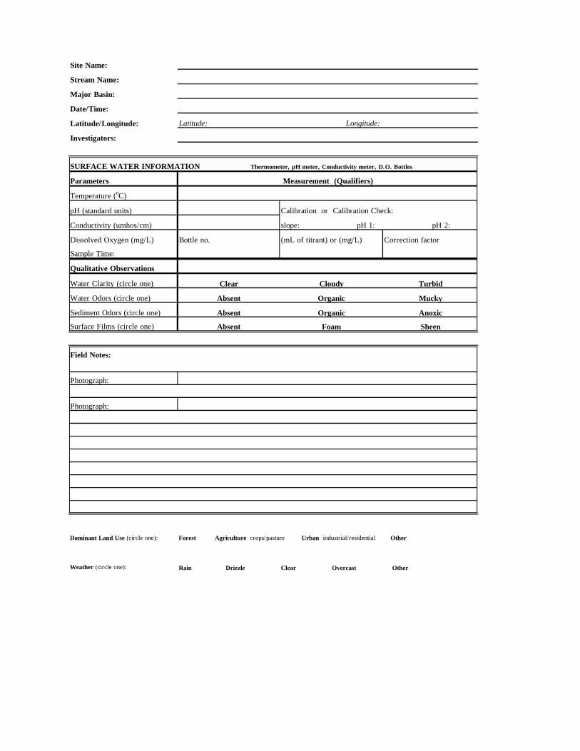
Site Name:

Stream Name:

Major Basin:

Date/Time:

Latitude/Longitude: Latitude: Longitude:

Investigators:

SURFACE WATER INFORMATION Thermometer, pH meter, Conductivity meter, D.O. Bottles

Parameters Measurement (Qualifiers)

Temperature (oC)

pH (standard units) Calibration or Calibration Check:

Conductivity (umhos/cm) slope: pH 1: pH 2:

Dissolved Oxygen (mg/L) Bottle no. (mL of titrant) or (mg/L) Correction factor

Sample Time:

Qualitative Observations

Water Clarity (circle one) Clear Cloudy Turbid

Water Odors (circle one) Absent Organic Mucky

Sediment Odors (circle one) Absent Organic Anoxic

Surface Films (circle one) Absent Foam Sheen

Field Notes:

Photograph:

Photograph:

Dominant Land Use (circle one): Forest Agriculture crops/pasture Urban industrial/residential Other

Weather (circle one): Rain Drizzle Clear Overcast Other

STREAM REACH PROFILE

Channel Feature Riffle 1 Riffle 2 Riffle 3 Riffle 4

(riffles) (riffles) (riffles) (riffles)

Wetted Width (m)

Bankfull Width (m)

Maximum Depth (m)

Gradient (%)

RPD (m)

Residual PoolD h

: Dp=maximum depth ofl

Dc=depth at pool crest (oril )

RPD=residual pool depth (Dp-D RPD)

CANOPY COVER MEASUREMENTS Equipment: Canopy Densiometer

DENSIOMETER (count open intersections)

Direction Riffle 1 Riffle 2 Riffle 3 Riffle 4

Center (up)

Center (down)

Center (left)

Center (right)

Left BankRight Bank

SUBSTRATE MEASUREMENTS Equipment: Glass-bottom bucket, Gridded hoop

Substrate Parameter Riffle 1 Riffle 2 Riffle 3 Riffle 4

Depth (meters)

Size Class (# intersections) Bedrock (smooth)

Bedrock (rough)

Boulder (250 to 4000 mm)

Cobble (64 to 250 mm)

Coarse Gravel (16 to 64 mm)

Fine Gravel (2 to 16 mm)

Sand (0.06 to 2 mm)

Silt/Clay/Muck (not gritty)

Wood (any size)

Other (comment)

Substrate measurements are made with a 60 cm diameter hoop and 50 equidistant observations

CURRENT VELOCITY Equipment: Wading rod and Flow meterLocation in Water Column Riffle 1 Riffle 2 Riffle 3 Riffle 4

Bottom of Stream0.6x Depth from Surface

Equipment: Measuring tape, Clinometer, Wading Rod

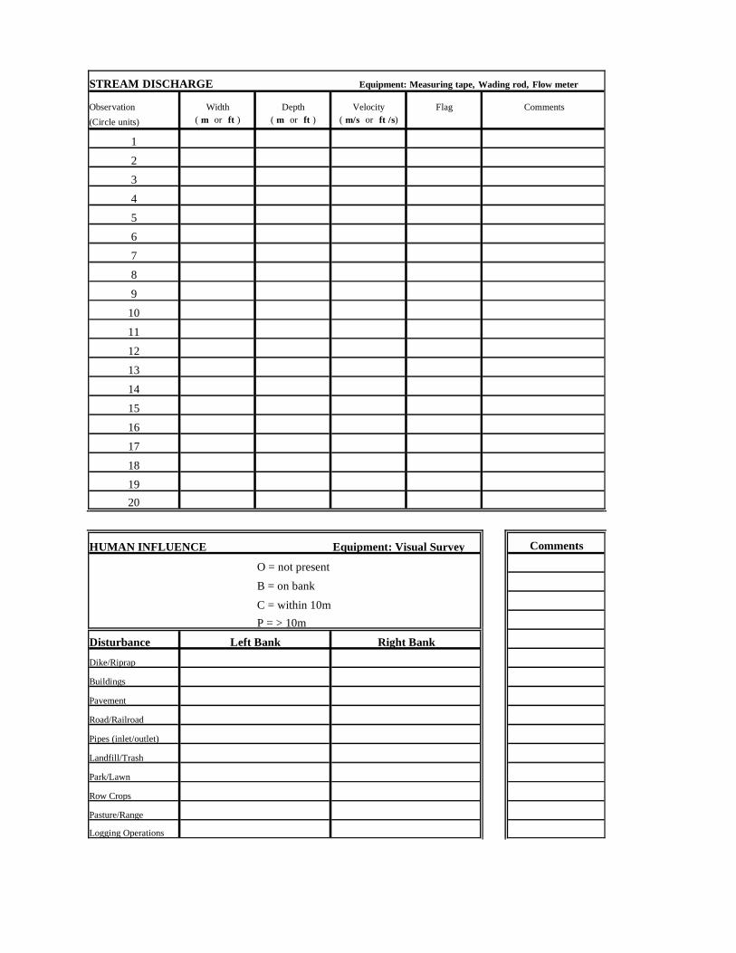
STREAM DISCHARGE Equipment: Measuring tape, Wading rod, Flow meter

Observation Width Depth Velocity Flag Comments(Circle units) ( m or ft ) ( m or ft ) ( m/s or ft /s)

123456789

1011121314151617181920

HUMAN INFLUENCE Equipment: Visual Survey Comments

O = not presentB = on bankC = within 10mP = > 10m

Disturbance Left Bank Right Bank

Dike/Riprap

Buildings

Pavement

Road/Railroad

Pipes (inlet/outlet)

Landfill/Trash

Park/Lawn

Row Crops

Pasture/Range

Logging Operations

SUBSTRATE MEASUREMENTS- PEBBLE COUNTSSize Class (mm) Riffle 1 Riffle 2 Riffle 3 Riffle 4≥ 512≥ 256≥ 180≥ 128≥ 90≥ 64≥ 45≥ 32≥ 22≥ 16≥ 11≥ 8≥ 6≥ 4≥ 2< 2

Equipment List

Biological Surveys

D-frame kick nets (2)Scrub brush (2)Cable ties (20)Field Preservative (85% denatured

ethanol)- 5 gallonsOne liter Polycarbonate containers (40)One gallon Heavy Duty freezer bags (30)Hip wadersChest wadersWader repair kitLabels (40)Fine tip permanent markers (2)Camera (1)Slide film (2 rolls)

Habitat Surveys

Field forms for each site150 ft tape measure (1)Fiberglass stadia rod (1)Clinometer (1)Compass (1)Flow meter (1)Spare batteries for meter (2)Flow rod (1)Substrate grid (1)

Plexiglass substrate viewer (1)Densiometer (1)GPS unit (1)“A Good Eye!”

Water Quality Surveys

250 ml water collection bottles (2)Alcohol thermometers (2)PH meter (1)Conductivity meter (1)Spare batteries for meters (2)Winkler dissolved oxgen bottles/Tray (12

bottles)Winkler reagentsDe-Ionized water (2 ½ gallons)Buffer Solutions (pH 4, ph 7, pH 10)10% Hydrochloric Acid (250 ml)

Personal Gear

Elbow Length Insulated GlovesRain GearLeather glovesField vestEyewash kitFirst aid kitDrinking Water

Benthic Macroinvertebrate Biological Monitoring Protocols ... · Benthic Macroinvertebrate...

Documents

Transcript of Benthic Macroinvertebrate Biological Monitoring Protocols ... · Benthic Macroinvertebrate...