Essays on Warehouse Operations · The first paper considers a material handling system with...
137
Essays on Warehouse Operations by Peter Bodnar A Ph.D. thesis submitted to the School of Business and Social Sciences, Aarhus University, in partial fulfillment of the Ph.D. degree in Economics and Business July 2013
Transcript of Essays on Warehouse Operations · The first paper considers a material handling system with...
Essays on Warehouse Operations
by
Peter Bodnar
A Ph.D. thesis submitted to the
School of Business and Social Sciences, Aarhus University,
in partial fulfillment of the Ph.D. degree in Economics and Business
July 2013

Members of the committee
Prof. Dr. Nils BoysenFriedrich-Schiller-Universität Jena, Germany
Professor Stefan RøpkeTechnical University of Denmark, Denmark
Associate Professor Marcel Turkensteen (Chairman)Aarhus University, Denmark
Date of the public defense
25 October 2013

Summary
The thesis consists of three papers related to the warehousing industry.
A dynamic programming algorithm for the space allocation and aisle positioning
problem. The first paper considers a material handling system with gravity flow racks and
addresses the problem of minimizing the total number of replenishments over a period subject
to practical constraints related to the need for aisles granting safe and easy access to storage
locations. In this paper, an exact dynamic programming algorithm is proposed for the problem.
The computational study shows that the exact algorithm can be used to find optimal solutions
for numerous SAAPP instances of moderate size.
Scheduling in a cross-dock environment to minimize mean completion time.
The second paper studies the problem of minimizing the mean completion time of outbound
trucks in a cross-dock environment with a single inbound door and a single outbound door.
Minimizing mean completion time improves the cross-dock’s responsiveness and is known to
lead to stable or balanced utilization of resources, and reduction of in-process inventory. The
problem is addressed from a flow shop scheduling perspective and its similarities with the
classical F2||∑Cj problem are exploited. Indeed, the problem is a generalization of F2||∑Cj ,
which is known to be NP-hard. A branch-and-bound algorithm is proposed to find an optimal
solution to the problem. Computational results show that the branch-and-bound algorithm
can optimally solve problem instances of moderate size within a reasonable amount of time.
Scheduling trucks in a cross-dock with mixed service mode dock doors. The
problem considered in the third paper is to schedule inbound and outbound trucks subject
to time windows at a multi-door cross-dock in which an intermixed sequence of inbound and
outbound trucks can be processed at the dock doors. The focus is on operational costs by
considering the cost of handling temporarily stored products, as well as the cost of tardiness
due to processing outbound trucks after their respective due dates. A mathematical model for
optimal solution is derived and an adaptive large neighborhood search heuristic is proposed to
compute near-optimal solutions of real size instances. Computational experiments show that
the proposed heuristic algorithm can obtain high quality solutions within short computation
times.
iv

Preface
This thesis was prepared at the School of Business and Social Sciences, Aarhus University
in partial fulfillment of the requirements for acquiring the Ph.D. degree in Economics and
Business. The work was carried out at the Department of Economics and Business.
The thesis extends the literature by proposing an exact algorithm for a known warehousing
problem and introducing two new research problems within the area of cross-dock operations.
The thesis considers exact and heuristic solution methods to solve the problems.
Three research papers are included in the thesis, of which one has been accepted for publi-
cation. In addition to the three papers, there is a supplementary report, which contains further
background and details for the application environment.
Acknowledgments
This thesis would not have been possible without the support of many people. It is a pleasure to
be able to express my gratitude to everyone who has given much valued support and assistance
to enable me to complete this thesis.
Foremost, I am greatly indebted to Professor Jens Lysgaard for all the time and attention
he has devoted as my supervisor. His invaluable advice and suggestions have been the keys to

the completion of this Ph.D. thesis. Jens Lysgaard is a prominent scientist and a great person:
it is for me an immense honor to be his student.
The external stay of my Ph.D. was spent at the Rotterdam School of Management, Erasmus
University, and I wish to thank Professor René de Koster for being a fantastic inspiration for my
work and for giving me the opportunity to work with him as a co-author. I would at the same
time like to thank him and the research group for making my visit a pleasant experience, as
well as the Købmand Ferdinand Sallings Mindefond from the Dansk Supermarked for providing
the funding.
I would like to extend my gratitude to all members of the Cluster of Operations Research
and Logistics (CORAL) at Aarhus University. It is an honor for me to be part of this research
group, which has produced a great number of eminent theoretical and practical contributions
in the field of operations research. In particular, I would like to thank Kim Allan Andersen,
Christian Larsen, Sin C. Ho, Michael Malmros Sørensen, Marcel Turkensteen, Hartanto Wijaya
Wong, and Sanne Wøhlk, for their comments, advice, and insights.
On a more personal basis, I wish to thank Soheil Abginehchi, Jeanne Andersen, Maria Elbek
Andersen, Lukas Bach, Lene Gilje Justesen, David Sloth Pedersen, Dominyka Sakalauskaite,
Jelmer van der Gaast, Nima Zaerpour, and all the friends at the Ph.D. corridor, for many
stimulating discussions, support and fun throughout these three years.
I am grateful to my family for their love and support: my mother Anna, my father Mihály,
my sister Erika ... and Cecilia, the woman I am so happy and proud to share my life with.
I should confess that her patience, help, and unselfish devotion make it possible to overcome
formidable challenges throughout my life and career.
Sincerely,
Peter Bodnar
Aarhus, July 2013.
vi
Contents
Summary iii
Preface v
Acknowledgments . . . . . . . . . . . . . . . . . . . . . . . . . . . . . . . . . . . . . . v
Contents vii
1 Introduction 1
1.1 Warehouse design . . . . . . . . . . . . . . . . . . . . . . . . . . . . . . . . . . . 4
1.2 Operations . . . . . . . . . . . . . . . . . . . . . . . . . . . . . . . . . . . . . . . 7
1.3 Outline of the thesis . . . . . . . . . . . . . . . . . . . . . . . . . . . . . . . . . 16
2 A Dynamic Programming Algorithm for the Space Allocation and Aisle
Positioning Problem 19
2.1 Introduction . . . . . . . . . . . . . . . . . . . . . . . . . . . . . . . . . . . . . . 21
2.2 Problem description . . . . . . . . . . . . . . . . . . . . . . . . . . . . . . . . . . 23
2.3 Modelling . . . . . . . . . . . . . . . . . . . . . . . . . . . . . . . . . . . . . . . 25
2.4 A dynamic programming algorithm . . . . . . . . . . . . . . . . . . . . . . . . . 30
2.5 Computational experiments . . . . . . . . . . . . . . . . . . . . . . . . . . . . . 38
2.6 Conclusions . . . . . . . . . . . . . . . . . . . . . . . . . . . . . . . . . . . . . . 42
3 Scheduling in a Cross-Dock Environment to Minimize Mean Completion
Time 43
3.1 Introduction . . . . . . . . . . . . . . . . . . . . . . . . . . . . . . . . . . . . . . 44
3.2 Problem description . . . . . . . . . . . . . . . . . . . . . . . . . . . . . . . . . . 46
3.3 Optimality properties . . . . . . . . . . . . . . . . . . . . . . . . . . . . . . . . . 50
3.4 Lower bounds . . . . . . . . . . . . . . . . . . . . . . . . . . . . . . . . . . . . . 54
3.5 Branch-and-bound . . . . . . . . . . . . . . . . . . . . . . . . . . . . . . . . . . 60
3.6 Computational experiments . . . . . . . . . . . . . . . . . . . . . . . . . . . . . 68
3.7 Conclusions . . . . . . . . . . . . . . . . . . . . . . . . . . . . . . . . . . . . . . 74
4 Scheduling Trucks in a Cross-Dock with Mixed Service Mode Dock Doors 77
4.1 Introduction . . . . . . . . . . . . . . . . . . . . . . . . . . . . . . . . . . . . . . 79
4.2 Literature review . . . . . . . . . . . . . . . . . . . . . . . . . . . . . . . . . . . 81
4.3 Problem description . . . . . . . . . . . . . . . . . . . . . . . . . . . . . . . . . . 85
4.4 Model formulation . . . . . . . . . . . . . . . . . . . . . . . . . . . . . . . . . . 87
4.5 Metaheuristic approach . . . . . . . . . . . . . . . . . . . . . . . . . . . . . . . . 93
4.6 Computational experiments . . . . . . . . . . . . . . . . . . . . . . . . . . . . . 104
4.7 Conclusions . . . . . . . . . . . . . . . . . . . . . . . . . . . . . . . . . . . . . . 111
Bibliography 113
viii
Chapter 1
Introduction

Warehouses are essential components of any supply chain. In a warehouse items are handled
in order to level out the variability and imbalances of the material flow caused by factors such as
seasonality in demand, production scheduling, transportation, and consolidation of items (Gu
et al., 2007). Inventories in warehouses are capital intensive assets that require storage areas,
handling equipment, and information systems. In addition, warehouse operations are repetitive,
labor intensive activities. The capital and operating costs of warehouses represent about 20-
25% of the logistics costs (Frazelle, 2002; Baker and Canessa, 2009). Therefore, improvements
in the planning and control of warehousing systems can contribute to the success of any supply
chain.
A warehouse is typically divided into functional areas that are designed to facilitate the
material flow (Tompkins et al., 2010). The main warehouse areas are outlined in the following:
receiving area, reserve and forward storage area, and shipping area. Operations in the receiving
area include the processing (i.e., unloading) of carriers, item identification, and quantity and
quality inspection. Received items are then moved to a storage area or directly to the shipping
area. The storage area is often divided into a reserve and a forward storage area. The reserve
storage area covers typically distant and heavily accessible locations, e.g., the uppermost part
of a rack, and is used to ensure the replenishment for the forward storage area. Customer
demand is primarily satisfied from the forward storage area, where the items are typically
stored in convenient size and the storage locations are easily accessible. In the shipping area,
items are sorted, consolidated and loaded on the carriers. While this is a general material flow
in a warehouse, the actual material flow depends mainly on the role of the particular warehouse
in the supply chain.
Specialized warehouses are established to fulfill the different requirements, e.g., production
warehouse, distribution warehouse, and cross-dock. The main function of a production ware-
house is buffering and storage, it supplies raw or semi-finished material for production and
may prepare finished items for shipment; the typical objective is the minimization of operation
and investment costs given the storage capacity and response time (Rouwenhorst et al., 2000).
2

Distribution warehouse (or distribution center) handles, in addition, the distribution of items.
In this case, the general objective is to achieve high throughput at minimum operational and
investment costs. In a cross-dock (or transshipment center), storage is scarcely presented, in-
coming items are immediately sorted and new customized shipments are created (De Koster
et al., 2007).
In a typical warehouse 65% of the operating expenses are consumed by order picking (Ruben
and Jacobs, 1999), which includes the item picking to replenish the forward area and to ful-
fill customer order. Therefore, this thesis focuses on those decision problems and warehouse
systems that aim to reduce or even eliminate the order picking costs. Chapter 2 addresses a
problem of minimizing the number of items picked to replenish the forward storage area during
the planning horizon. The problem has been introduced by Anken et al. (2011), and a heuristic
algorithm has been proposed to obtain near-optimal solutions. The study presented in chapter
2 extends the existing literature and proposes an exact algorithm.
However, order picking costs can be further reduced by directly moving items from the
receiving to the shipping area, that is, by cross-docking. Two studies presented in chapter 3
and 4 consider cross-dock environments and address the problem of scheduling inbound and
outbound trucks. The truck scheduling problem emerges when the number of docks is less than
the number of trucks that are available to be processed. In chapter 3, an exact algorithm is
proposed to the case when the performance criterion is the mean completion time of outbound
trucks. In chapter 4, the objective is to minimize the operation costs which consist of the
following: the storage and retrieval costs and the tardiness costs.
In the remaining part of this chapter, further background information and details are pro-
vided for the application environment. Many studies propose a framework to classify the
existing literature on warehousing. These frameworks are based on either application areas,
methodology, levels of decision, or a combination of these. One of the first literature reviews is
presented by Matson and White (1982); their framework is based on application areas such as
transfer lines, flexible manufacturing, and order picking systems. van den Berg (1999) focuses
3
also on application areas and reviews the research on storage and order picking. A study by
De Koster et al. (2007) considers low-level, picker-to-parts order-picking systems in a frame-
work that classify the literature based on the different levels of decisions. Ashayeri and Gelders
(1985) propose a framework based on the solution approach and distinguish exact, approximate,
and simulation methods. Wäscher (2004) classify the literature based on both application area
and solution approach. Cormier and Gunn (1992) presents a comprehensive study that clus-
ters literature based on the level of decisions. Rouwenhorst et al. (2000) propose a framework
based on decision levels, material flow, and organization aspects. Recently, Gu et al. (2007,
2010a) present two studies, which cover warehouse operations and design, respectively, with an
outlook to performance evaluation. In this chapter, the considered warehousing decisions are
structured in a framework that first clusters the problems based on the levels of decisions, and
then (where appropriate) the subproblems are addressed in a sequence that follows the typical
material flow.
The structure of this chapter is the following. Section 1.1 presents high-level warehouse
design decisions, which establish the overall structure and define the functional areas. Section
1.2 elaborates on the operation decisions that define the details of the material and information
flow. These decisions are at a tactical level for one organization and at an operational level
for another depending on the particular characteristics of the organization. The problems ad-
dressed in this thesis are connected to operations decisions. Section 1.3 presents the motivation
of the research and provides an outline for the following chapters.
1.1 Warehouse design
Warehouse design is often tackled by a stepwise approach with interrelated phases and frequent
reiteration (Baker and Canessa, 2009). The overall structure of a warehouse design is deter-
mined by the role of the given warehouse in the supply chain. This role defines the business
requirements and key focus areas, as well as the constraints on the design. Based on the assem-
4
bled and analyzed data, operation principles and stock keeping units (SKUs) are defined which
aid managers reducing the range of feasible configurations. An SKU serves as an alphanu-
meric product number to identify and keep track of the stored items; each item is assigned an
SKU number based on its characteristic (Tompkins et al., 2010). According to Rouwenhorst
et al. (2000) the next phase is to develop functional specifications and operating procedures.
The priorities in this phase are established by taking into account the performance evaluation,
which is traditionally production and cost oriented, e.g., maximize throughput and minimize
total discounted cost. Ashayeri et al. (1985) present a model that seeks to minimize the sum
of investment and operation costs in automated warehousing systems subject to constraints
on throughput, warehouse size, and crane capacity. According to Goetschalckx and Ashayeri
(1989), customer oriented objectives are increasingly pursued, e.g., minimize mean processing
time (De Koster and Van der Poort, 1998; Jarvis and McDowell, 1991), or minimize tardiness
(Chan and Kumar, 2009). The problem of finding a trade-off between the objectives emerges
often in the presence of both production and customer oriented objectives. For instance, Kovács
(2011) shows the contradiction between minimizing the maximum of response time (also called
order cycle time) and minimizing the average response time (also called average picking time).
Warehouse design decisions address also equipment selection and internal arrangement de-
cisions, which cover the allocation of functional areas that exhibit various configurations in
terms of size, layout, and procedures (Pliskin and Dori, 1982; Heragu et al., 2005). Ashayeri
and Gelders (1985) provide a literature review on various methods that can assist with the
evaluation of equipment types. Size and dimension related decisions are influenced by expected
inventory levels, which establish the maximum capacity and define the resource requirements
(Francis and White, 1992). The warehouse sizing problem has been addressed by Goh et al.
(2001). They model a warehousing cost with a piecewise linear function assuming a multi-
SKU system and provide an exact algorithm for the case of separable inventory costs and an
approximation algorithm for the case of joint inventory costs.
A storage area is often divided into a reserve and a forward area (Tompkins et al., 2010).
5
The problem of sizing these areas has been addressed in the papers by Bhaskaran and Malmborg
(1990) and Malmborg (1996a) with a stochastic cost-savings model and an integrated evaluation
model, respectively. These models can be used to evaluate different scenarios. The paper
of Hackman et al. (1990) is among the earliest studies on modeling the product allocation
problem (also called forward-reserve allocation problem), that is, the problem of determining
which product to place in the forward storage area and in what quantities. A greedy heuristic
is proposed to solve the problem based on a prior ranking of the products. Hackman and
Platzman (1990) provide a mixed integer linear programming formulation to address more
general instances of the above problem. van den Berg et al. (1998) provide a knapsack based
heuristic assuming unit-load replenishment. For the base problem, Gu et al. (2010b) provide a
branch-and-bound algorithm.
In a storage area, products are allocated to storage locations, which are organized in single-
block or multi-block layout where longitudinal and cross aisles separate the blocks. That is, a
block is a group of compartments, e.g., conventional fix racks or bin cabinets. Recently, mobile
and flexible systems are also available, e.g., gravity flow rack and rail-embedded motorized
rack. Bassan et al. (1980) present some optimal design parameters for determining the internal
layout of storage bays in a rectangular-shaped warehouse. Rosenblatt and Roll (1984) extend
the work of Bassan et al. (1980) and propose a simulation based procedure that integrates the
warehouse sizing problem, and the internal layout problem. Input/output (I/O) point (also
referred as pickup and drop-off point) is the location, where goods arrive and leave the storage
area. The distance between the I/O point and a storage location has an essential effect on the
time required to store or retrieve an item assigned to that particular location. The traditional
layout is commonly referred to as rectangle-in-time, which refer to the shape of the isolines that
are computed to identify locations at identical distances from the nearest I/O point. Recently,
Gue and Meller (2009) and Gue et al. (2012) present novel aisle designs, e.g., ‘flying-V’ and
‘fishbone’, with the aim to reduce the travel time by relaxing the conventional requirement
of parallel picking aisles and orthogonal cross aisles. The results show that the total travel
6

time can be reduced by enabling non-orthogonal cross aisles and orienting the picking aisles in
different directions. However, the reduction decreases as the number of I/O points increases.
Proposed warehouse design solutions are finally evaluated and assessed. Scenarios are often
constructed to consider various situations and configurations; decisions in this phase can be
facilitated with simulation models (Baker and Canessa, 2009). These models may also include
operation decisions, which are presented in the following section.
1.2 Operations
Operation decisions define the material flow in a warehouse, which is elaborated in the following.
First, items arrive and received in the facility. Then the item is either forwarded to the shipping
area or allocated in a storage location. The best storage location is close to a dock so that the
cost of (i) unloading the items at a dock and transporting them to the storage area and (ii)
accessing items and transferring them to a dock for loading is minimized. As a result, items
compete for storage locations that are closest to the docks (Ahuja et al., 1993). When an order
is received, the picker retrieves the ordered items. Note that the retrieval can be triggered
either by an order for item replenishment in the forward storage area or by a customer order.
To ensure efficiency, the picker should follow a route that minimizes the cost of the retrieval.
Order consolidation can be considered to facilitate an efficient picking. The sorting is necessary
if items have to be clustered by customer order after the completion of the picking (De Koster
et al., 2007). Finally, items are loaded on the carriers and shipped. The main stages in this
process are: receiving, storage, order picking, and shipping.
1.2.1 Receiving and shipping
Receiving and shipping are warehouse operations, which represent two extreme connection
points of the warehouse procedures. Receiving includes typically carrier processing (i.e., un-
loading), item identification, recording the goods receipt, quantity and quality inspection, un-
7

packing, and sorting activities; whereas, shipping includes finishing, batching, packing, and
loading operations.
The truck-to-dock assignment problem emerges in multi-door warehouses, where a set of
docks are available to process a set of carriers and the problem is to assign the docks to the
carriers so that some performance criteria are met. The paper of Tsui and Chang (1990) is
among the first studies on the truck–to–dock assignment problem with the objective to minimize
total travel time inside the facility. The authors present a bilinear objective formulation and
provide a local search algorithm. For the same formulation, Tsui and Chang (1992) describe
a branch-and-bound algorithm. The paper of Oh et al. (2006) presents the problem in the
context of a mail distribution center and proposes a genetic algorithm heuristic. Miao et al.
(2009) consider the problem with operational time constraints assuming that trucks are pre-
scheduled with hard time windows during which a dock is fully occupied; tabu search and a
genetic algorithm are proposed in the paper.
When several trucks are to be processed at a facility with limited number of docks, the
truck scheduling policy determines the order of trucks. That is, the truck scheduling problem
is the problem of defining the start and completion times for the processing of each truck so
that some performance criteria are met. In this problem, the time dimension is taken into
account; hence the objective function also tends to be time-related, such as the minimization of
makespan, defined as the completion time of the last outbound vehicle. (Boysen and Fliedner,
2010). For excellent reviews on truck scheduling the reader is referred to Agustina et al. (2010),
Boysen and Fliedner (2010) and Van Belle et al. (2012).
1.2.2 Storage
Storage is the process of allocating items in the warehouse. Since warehouse storage locations
and pickers are generally scarce resources, therefore high allocation efficiency is required in
terms of utilization of both picker effort and storage capacity. Storage includes the following
interrelated activities: sequencing and consolidation, storage location assignment, and shuffling.
8
Item sequencing determines the order, according to which items are sorted to be processed,
e.g., allocated or shuffled. Item sequencing is typically based on a first come, first served or on an
earliest due date order. However, items can be consolidated (or clustered) according to decisions
and restrictions determining whether different items can be placed in the same compartment.
A dedicated compartment accommodates only one item. While in a mixed compartment, more
items can be allocated. e.g., a stored pallet may consist of several different products, or a rack
location may cover several slots and a product can be assigned to each slot. Item consolidation
may yield both improved storage utilization and increased complexity (Anken et al., 2011).
Steudel (1979) presents a heuristic for the pallet loading problem, where units of a single
product are placed on a pallet forming a layout that minimizes the unused area. The problem
is formulated as a two-dimensional cutting stock problem, where the original area is partitioned
into sub-areas. Tsai et al. (1988) present stylized model with an LP formulation for the two-
dimensional palletizing problem with products of different size. However, item consolidation is
frequently limited by compliance restrictions among products or between product and location,
e.g., product-to-product restriction is common in industries where products can pollute or
damage each other (Heskett, 1964).
The storage location assignment policy determines where a given item is stored. The main
difference between the product allocation and the storage location assignment problems is
that the former considers the reserve and forward storage areas and product volumes, while
latter focuses typically on multiple locations and individual items. Storage location assignment
policies can be classified into two main groups, namely, dedicated and shared policies. Dedicated
storage location assignment commits compartments to products during the planning horizon.
This policy requires a high storage capacity to store the maximum inventory of each product
(Tompkins et al., 2010). However, once the products and the locations are matched, only the
quantity has to be updated at every transaction, therefore this policy improves the transparency
and the picker’s familiarity with the locations of the different products. Shared storage location
assignment allows the compartment to accommodate different products; therefore the location
9
may be potential for any product upon necessary capacity and product-location compliance.
This policy can be computationally intensive. However, the main advantage of it is that the
storage capacity required must only fulfill the peak inventory level of all products during the
planning horizon (Tompkins et al., 2010). That is, the storage capacity requirement with the
shared storage location assignment is lower.
Dedicated storage location assignment is commonly used to reduce the picking effort, since
related assignment methods, in general, place popular items to easily accessible locations;
thereby the average picking time is shortened. Shared storage location assignment is usually
applied in order to scale down the storage capacity requirement. The two assignments can be
compared based on picking effort and utilized storage space. Malmborg (1996b) shows that for
a given α/β ‘ABC-curve’, where α% of the stored items are responsible for β% of the retrieval
transactions, a skewness factor s = logα β indicates which one of the two policies may provide
superior performance. As the value of the s ∈ (0, 1) increases the advantage of the shared
policy decreases. When s = 1, all items have the same level of demand retrievals.
The storage location assignment influences essentially the expected total storage and order
picking time, which consists of travel time, stowing and retrieving time, and administration
related time. The travel time may take up to 50 % of the total time spent on storing and picking
an item (Francis and White, 1992). Therefore, several studies have addressed storage location
assignment problem with the objective to minimize the travel time. The storage location
assignment policies frequently considered in the literature are: random, closest-open-location,
popularity based, turnover based, class based, and duration-of-stay based (DOS) rule.
Random storage location assignment policy allocates items to locations with equal likelihood
resulting in leveled storage space utilization. When comparing the performances of different
methods, the random assignment is usually applied as a benchmark. In practice, items are
commonly allocated to the available compartment closest to the I/O point; this method is
called the closest-open-location policy. However, the performance of the closest-open-location
policy is often approximated by applying the random policy (De Koster et al., 2007).
10

Product characteristics can be incorporated in the decision to improve the performance.
Information about product popularity, which is the average number of retrieval orders during
the planning period, can be used to reduce expected storage and retrieve time. The most
frequently ordered product is assigned to the location closest to the I/O point, the second most
frequently ordered product to the second closest location, etc. Therefore high-runner items are
placed at the easiest accessible locations, while low-demand items are allocated farther, this
facilitates that the expected storage/retrieval time is low. However, such a policy may increase
aisle congestion and create unbalanced utilization.
Hausman et al. (1976) provide a seminal study on the full turnover-based assignment rule,
in which the highest-turnover item is assigned to the location closest to the I/O point, and show
that this approach offers superior performance with respect to the expected total travel time
compared to the closest-open-location rule. Turnover-based assignment can also be adopted in
a facility using a throughput-to-storage ratio (Liu, 2004), or a density-turnover index (Chuang
et al., 2012). Lee and Elsayed (2005) propose an iterative search procedure to determine the
space requirements for warehouse systems operating with a full turnover-based storage rule.
The inverse of the turnover rate of a product is called the cube-per-order index (COI), which
was first presented by Heskett (1963, 1964). The COI based policy is found to be optimal under
certain circumstances (Francis and White, 1992). Malmborg and Bhaskaran (1990) show the
optimality of the COI in a system where one storage and one retrieval is executed within a
picking cycle. Moreover, they consider the cases when the COI rule provides alternative layouts
and propose a heuristic to select one. Recently, Yu and De Koster (2013) present that when
full turnover-based storage is coupled with dedicated storage, then this policy does not always
outperform class-based and random storage assignment rule in terms of the expected travel
times.
Class-based storage assignment rule is a shared assignment policy which clusters products
into classes based on product characteristics, such as popularity or turnover. The item classes
are assigned to a group of storage locations. The class with the highest average popularity or
11
turnover is assigned to locations closest to the I/O group, and within the class the items are
conventionally assigned to random storage locations (Kulturel et al., 1999). The main proce-
dures, i.e., establishing the boundaries of the product classes and assigning storage locations
to these classes are done either simultaneously or in a cyclical manner. The selected item
attributes determine the development of distinguished classes. Rosenblatt and Eynan (1989)
show the decrease of marginal cost benefit when increasing the number of classes. Muppani
and Adil (2008a,b) present a branch-and-bound and a simulated annealing approach to form
storage classes considering storage-space cost and handling cost. To the case when demand
is stochastic, Ang et al. (2012) propose a robust optimization based approach to solve the
multi-period storage assignment problem.
Administrative cost can be reduced when items from the same shipment are grouped and
handled together (Roll and Rosenblatt, 1983). Frazelle and Sharp (1989) introduce the cor-
related assignment policy (also referred as family grouping) which can reduce both the time
required to locate the item and the interleaving time, which is the travel time between two
adjacent retrievals within the same picking cycle. The contact based correlation is based on the
frequency by which the items are picked sequentially (Garfinkel, 2005). Whereas, the comple-
mentary based correlation measures the strength of joint demand (Mantel et al., 2007). Chuang
et al. (2012) propose a model for the two-stage clustering-assignment problem assuming ded-
icated storage assignment policy and orders with multiple items. In the first stage, items are
clustered into groups based on the correlation between them. In the second stage, groups are
assigned to storage locations.
Goetschalckx and Ratliff (1990) present the DOS rule, which incorporates information about
each individual item and determines the storage location based on its duration-of-stay, which
is the expected time interval between the arrival (or storage) and the departure (or retrieval)
times of a given item. Kulturel et al. (1999) present a comparison between the class-based
full-turnover rule and the class-based DOS rule assuming three classes and stochastic demand.
The results show that the class-based full-turnover rule tends to provide superior results with
12
respect to total travel time.
However, it is possible to relax the traditional requirement that items are committed to the
locations, where they were once assigned to, until the retrieval of the last unit. Shuffling can
improve storage utilization of a warehouse by replacing the items. That is, a low-demand item
allocated close to the I/O point can be swapped with a high-runner item allocated further from
the I/O point, or similar items can be grouped in a new location. Jaikumar and Solomon (1990)
present a heuristic for the shuffling (or reallocation) problem, their approach assumes sufficient
slack time to perform the shuffling. The paper emphasizes the hierarchy of the problems. The
first problem is the long-term storage location assignment based on ex ante data, followed by
an optional reallocation problem, and finally a short-term storage location assignment problem
based on ex post data. In the paper of Muralidharan et al. (1995), the shuffling problem
is formulated as a precedence-constrained asymmetric traveling salesman problem, and it is
addressed by two heuristic methods. Sadiq et al. (1996) present an improvement heuristic for
dynamic warehouse environments. The heuristic aims to improve order picking and shuffling
time by incorporating expected demand and correlation among products.
1.2.3 Order picking
An order consists of a set of order lines, which indicate the product code and the required
quantity. Orders may be clustered to increase the efficiency of the retrieval; this is referred to
as order consolidation. A cycle is a route from the I/O point to the requested storage location(s)
and back to the I/O point. Single-command cycle policy (or single-address system) allows only
either one storage or one retrieval activity at a cycle. A single storage and a single retrieval
activity are combined in a dual-command cycle policy (or dual-address system). Finally, multi-
command cycle policy allows several storage and several retrieval activities within one cycle.
When multiple orders request the same product, the items can be picked in batches. In this case
sorting is required before delivering the items, i.e., the picked products are divided into smaller
quantities corresponding to the orders. Sorting can pursue a sequential or a simultaneous
13

approach (Roodbergen and Vis, 2006). The former is called pick-and-sort, i.e., sorting is done
after items have been accumulated during picking. The latter is called sort-while-pick, i.e.,
sorting is done during picking.
Order picking can be manual, mechanical or automatic. The configuration of picking sys-
tems, including the level of mechanization, may vary among different departments and product
groups. The main types of picking systems are the following: picker-less, picker-to-product,
and product-to-picker. A picker-less system is a completely automatic system, e.g., items are
loaded on a conveyor from an A-frame. In a product-to-picker system the item is transported
to the location of the picker, e.g., by using mini-load or carousel. In a picker-to-product system
a picker goes to the location of the product, retrieves it, and delivers it to an I/O point or he
may place the item on a conveyor belt, the latter case is called a pick-to-belt system (Anken
et al., 2011).
Picker-to-product systems can be divided into sequential and parallel picking processes.
In a sequential picking process only one picker works on an order. It can be further divided
into discrete (or single order) picking and batch picking depending on the number of orders
handled simultaneously by the picker. On the other hand, in a parallel picking process several
pickers may work simultaneously on the same order but on different order lines. To increase
the familiarity of the picker with the locations of the products, pickers can be assigned to
zones, which are groups of storage locations. In general, zones have determined boundaries;
therefore the order can be split based on the location of the ordered products. Jane and
Laih (2005) present a clustering model to construct a set of zones assuming a parallel picking
process. The problem isNP-hard, hence a heuristic approach is proposed for real size instances.
Parikh and Meller (2008) show that the workload-imbalance is greater in zone picking systems
when compared to the case that orders are first consolidated and then picked sequentially.
Bartholdi III et al. (2001) presents the advantages of a flexible setup based on sequential picking,
called the bucket-brigade policy, where pickers work in a line and as soon as one becomes idle
he moves up the line and takes over the order from an adjacent picker. Simulation results show
14

that if walking time is insignificant, then the bucket-brigade policy can increase production
rate and balance the workload among the pickers.
Picker-to-product systems are traditionally connected to pick-to-paper systems, where the
orders are printed, and the picker follows the instructions on the hard copy. However, pick-
to-light and pick-to-voice (or pick-by-voice) systems are also available, in these cases the items
are indicated by light or the picker is informed via radio, respectively. In a manual or semi-
mechanical picker-to-product system the picker is typically a warehouse employee with a picking
cart or a vehicle, whereas in a heavily-mechanical or automated picker-to-product system the
picker may be a crane. There is an extensive literature on semi-automatic and fully automatic
storage systems. Sarker and Babu (1995) provide a literature review on automated storage and
retrieval systems. Johnson and Brandeau (1996) extend the review by including automated
guided vehicle systems. Recently, a comprehensive literature review is presented by Roodbergen
and Vis (2009).
The order-picking problem (or retrieval sequencing problem) is to find the sequence of re-
trievals for a set of orders in a multi-command system which minimizes the travel time. The
sequencing and routing of pickers can be established by individual or standardized policies (Pe-
tersen II and Schmenner, 1999). Individual routing policy determines the sequence of visited
locations for each storage/retrieve cycle regardless of previous routes. Ratliff and Rosenthal
(1983) show that the order-picking problem is a variant of the traveling salesman problem,
and propose a network flow model in which the vertices represent the ordered items locations,
the aisle ends, and the I/O points. Due to the complexity of establishing individual routes,
the sequence of visited locations are often developed based on a selected heuristic algorithm
(Petersen II, 1999; Roodbergen, 2001), e.g., transversal, largest gap, and composite. When the
transversal (or S-shape) method is applied the picker enters the aisle containing a pick and
traverses it. In the largest gap method, the ‘gap’ is defined as the distance between any two
adjacent items, or between a cross-aisle and the nearest item. The picker enters each aisle,
which contains an ordered product, up to the largest gap and leaves the same direction as
15
she entered. A composite method combines the previous two methods. These methods are
frequently used in practice (Hall, 1993). Roodbergen and Vis (2006) consider the transversal
and largest gap methods and shows that their performance with respect to total travel distance
depends on the layout of the order picking area.
1.3 Outline of the thesis
This thesis focuses on warehouse operations. Order picking is known to be the most labor
intensive and costly activities in a warehouse (De Koster et al., 2007). Order picking arises
when items are picked to satisfy customer demand or to replenish the forward area. In a typical
warehouse environment, 65% of the total operating expenses are attributed to order picking
functions (Ruben and Jacobs, 1999). Therefore, improvements that facilitate the reduction of
order picking costs are of great interests.
In chapter 2, a study presented by Anken et al. (2011) is extended. The study considers
a distribution center with a reserve and a forward storage area, and focuses on reducing the
number of replenishments to ensure product availability over a period. The problem is called
the space allocation and aisle positioning problem (SAAPP). It addresses simultaneously two
important and interrelated problems, namely, the product allocation problem and the storage
location assignment problem. Anken et al. (2011) propose a two-phase heuristic algorithm
to obtain near-optimal solutions and a mathematical formulation that can be used with a
commercial software to obtain optimal solutions for small size instances. The complexity of
the SAAPP is due to practical requirements related to safe and easy access to the items in the
considered warehouse system, which is a picker-to-product pick-to-belt system with gravity flow
racks that composed of multiple locations and multiple slots per location. Chapter 2 focuses on
an exact approach for the SAAPP and provides an algorithm that can obtain optimal solutions
for instances of moderate size. The key contributions presented in this chapter are (1) a graph
representation of the problem, and (2) an exact dynamic programming algorithm.
16

However, order picking costs can be minimized or even eliminated in cross-docking facilities.
In a cross-dock, items arrive typically from several suppliers, unloaded from inbound trucks
and sorted so that items of one supplier can be consolidated with other supplier items for
common final delivery destinations. Then, the items are loaded on outbound trucks. During
this process, items are either moved directly from inbound to outbound trucks or stored in a
temporary storage (or buffer) area for a short time (Bartholdi III and Gue, 2004). The benefit
of cross-docking is that it can reduce order picking and inventory holding costs compared
to traditional warehousing, it can also reduce transportation costs and increase the capacity
utilization of the trucks compared to direct transportation between suppliers and customers.
However, cross-docking requires the planning of the docking activities and the scheduling of the
trucks. The truck scheduling problem emerges repeatedly during the daily cross-dock operations
and has a key role in a rapid transshipment process (Boysen and Fliedner, 2010). In this thesis,
chapters 3 and 4 consider truck scheduling problems in a cross-docking environment.
In chapter 3 the performance criteria is to minimize the mean completion time. This
objective is known to improve responsiveness and leads to stable or balanced utilization of
resources (Rajendran and Ziegler, 1997; Framinan and Leisten, 2003). Moreover, it can facilitate
a high turnover of items and the timely completion of trucks processed at the cross-dock. Some
properties of the problem are described and an exact algorithm is proposed to obtain solutions
for instances of moderate size. The key contributions in this chapter are (1) the identification of
some optimality properties, (2) the valid bounding procedures and dominance criteria, and (3)
a branch-and-bound algorithm that is able to obtain optimal solution for instances of moderate
size.
Finally, in chapter 4 the investigated truck scheduling problem considers explicitly both
the order picking costs and the timely completion of trucks. The performance criterion of the
problem is to minimize the operational costs, consisting of storage, retrieval, and tardiness costs.
The cost of storage and retrieval relates to those items that are placed in the temporary storage
area instead of being directly loaded on the outbound trucks. The problem is shown to be NP-
17

hard therefore for large size instances a heuristic algorithm is proposed. In this chapter, the
key contributions are (1) a mathematical model that can be used to solve instances of moderate
size, (2) a proof of problem complexity, and (3) a heuristic algorithm that can be used to obtain
near-optimal solutions for large instances.
18

Chapter 2
A Dynamic Programming Algorithm for the
Space Allocation and Aisle Positioning Problem
A Dynamic Programming Algorithm for theSpace Allocation and Aisle Positioning Problem
Peter Bodnar and Jens Lysgaard
CORAL, Department of Economics and Business, Aarhus University, Denmark
[email protected] and [email protected]
Abstract
The space allocation and aisle positioning problem (SAAPP) in a material handling
system with gravity flow racks is the problem of minimizing the total number of replenish-
ments over a period subject to practical constraints related to the need for aisles granting
safe and easy access to storage locations. In this paper, we develop an exact dynamic
programming algorithm for the SAAPP. The computational study shows that our ex-
act algorithm can be used to find optimal solutions for numerous SAAPP instances of
moderate size.
This paper has been accepted for publication in the Journal of the Operational Research Society.
The contribution is reprinted with permission: Bodnar, P. and Lysgaard, J. (2013). A dynamic
programming algorithm for the space allocation and aisle positioning problem. Journal of the
Operational Research Society. doi:10.1057/jors.2013.64
20
2.1 Introduction
Storage locations are often grouped into a forward area and a reserve area; customer demand is
primarily satisfied from the forward area, where the products are typically stored in convenient
size and the storage locations are easily accessible. The reserve area covers typically distant
and heavily accessible locations, e.g., an external warehouse or the uppermost part of a rack,
and is used to ensure the replenishment for the forward area (Tompkins et al., 2010).
In the forward area, a picker-to-product, pick-to-belt system may be utilized, which enables
the order picker to walk down the line removing cases from pallet storage locations and placing
them on a take-away belt or roller conveyor; such a system provides high picking productivity
and less travel distance between picks (Frazelle, 2002). In order to further increase efficiency
by decreasing travel time/distance, products can be stored on a gravity flow rack (Gu et al.,
2010a), which is a storage rack with deep locations that utilizes rollers to ‘flow’ the products
from the back of the location to the front, thereby making the products more accessible for
small-quantity order picking. This is a first-in, first-out (FIFO) storage system that provides
high throughput pallet storage and retrieval as well as efficient space utilization (Frazelle, 2002).
In a gravity flow system, a dedicated location accommodates only a single product, and it
requires a single access point from the front, thus a dedicated location is both simple and space
efficient. A location with multiple commodities is referred as a mixed location; the maximum
number of different products stored at a mixed location is equal to the number of slots (i.e., the
depth of the location). A mixed location can increase the number of different products stored
on a gravity flow rack; however, it requires an access point from the side so that the picker can
reach any of the products. Gravity flow systems are capital intensive, hence efficient utilization
is essential.
In such a warehouse system, the space allocation and aisle positioning problem (SAAPP) is
defined by Anken et al. (2011) as the problem of minimizing the total number of replenishments
over a period subject to some intuitive and practical constraints related to the need for aisles
granting safe and easy access to storage locations. The defined problem includes an advance
21
replenishment period, in which the forward area can be replenished while no product is re-
trieved. The SAAPP considers two interrelated problems and seeks to find an optimal solution
for them simultaneously. The first is the determination of the number of units per product
allocated to the forward area. The second problem is the storage location assignment problem.
Separately, these problems have been extensively investigated. For a literature review we refer
to Rouwenhorst et al. (2000), Wäscher (2004) and Gu et al. (2007).
However, previous research in the field of material handling seems to underestimate the
effect of interrelations between the managerial decisions on warehouse performance. It is thus
of interest to learn how material handling decisions are interconnected, and develop integrated
material handling systems. Need for research on integration of problems has been expressed
earlier in Matson and White (1982) and De Koster et al. (2007).
In this paper, we define the SAAPP as a shortest path problem with resource constraints
on an appropriately defined graph and introduce a dynamic programming algorithm for its
solution. Similarly to Anken et al. (2011), we take the approach of addressing the SAAPP
with the equivalent objective of maximizing the number of allocated product units during the
advance replenishment period, instead of minimizing the total number of replenishments. The
correspondence of these two objectives is valid, since for each product the number of allocated
units is at most its periodic demand and any unit that is not allocated in advance must be
replenished during the period.
The main contribution of this research is our exact algorithm which is able to optimally
solve SAAPP instances of moderate size in reasonable time. Indeed, the instances that we are
able to solve to proven optimality are considerably larger than those solved in Anken et al.
(2011).
In the following, we first briefly describe the problem along with an illustrative example.
Thereafter we present our modelling of the problem, in particular we introduce a graph rep-
resentation of the SAAPP where any feasible solution is given as a directed path between a
specified pair of vertices in the graph. Further, we present our dynamic programming algorithm
22
for finding an optimal path in this graph. Then, the results of the computational experiments
are reported. Finally, the conclusion is presented.
2.2 Problem description
The SAAPP is to maximize the number of allocated product units (or, equivalently, minimizing
the total number of replenishments over a period), given a unit-load, gravity flow storage
system with n locations, m slots per location, p different products with a periodic demand
dj (j = 1, . . . , p) and the following requirements according to Anken et al. (2011): (i) each
product receives at least one slot, (ii) each mixed location is adjacent to an empty location
(i.e., an empty aisle), (iii) all allocated units of a product are located in the minimum number
of consecutive locations and (iv) all units of a given product are located on only one side of an
empty location. Moreover, it is given in the problem formulation by Anken et al. (2011) that
the solution focuses on the advance replenishment, which is distinguished from replenishment
during the period as in van den Berg et al. (1998), and that the periodic demand is stated in
unit-loads.
Figure 2.1 illustrates a gravity flow system with pallet loads, case picking, 4 locations and
4 slots per location.
As an example, we may consider a system with n = 4, m = 4, and p = 5. The products
are named A, B, C, D, and E with respective demand values 2, 2, 3, 4, and 5. We shall present
five solutions in Figure 2.2, out of which four are infeasible due to constraint violation and
only one is feasible. We depict a simple storage system viewed from above, as in Figure 2.1b.
The empty storage slots are indicated with diagonal stripe pattern. Figure 2.2a depicts an
infeasible solution since it contains two mixed locations (1 and 2) without an empty aisle. In
Figure 2.2b, location 1 is mixed without an adjacent empty aisle. In Figure 2.2c, the solution is
infeasible because product C is stored in two non-consecutive locations (1 and 3) on both sides
of an empty location. In Figure 2.2d, product C is missing which makes the solution infeasible.
23

(a) View from an angle (b) View from above
Figure 2.1: An industrial gravity flow storage system
Finally, Figure 2.2e presents a feasible solution which is also optimal for this example.
1 2 3 4
A C E D
A C E D
B C E D
B E E D
Slo
ts
Locations
(a) Missing aisle I
1 2 3 4
A D E
A C D E
B C D E
B C D E
Locations
Slo
ts
(b) Missing aisle II
1 2 3 4
A C E
B D E
C D E
C D E
Locations
Slo
ts
(c) Remote locations
1 2 3 4
A D E
A D E
B D E
B D E
Locations
Slo
ts
(d) Missing product
1 2 3 4
A C E
A D E
B D E
B D E
Locations
Slo
ts
(e) Feasible
Figure 2.2: Four infeasible solutions and one feasible solution for the example problem instance.
24
2.3 Modelling
In the following, we introduce our graph representation of the SAAPP. Then we eliminate
certain solution symmetries by clustering products. Further, we define a location’s status
according to whether the location is empty, mixed, or dedicated. Finally we present the solution
space and labels used in our dynamic programming algorithm.
2.3.1 Graph representation
Given the p products with demands d1, . . . , dp, a feasible solution may be characterized as
a vector of allocated quantities a1, . . . , ap, where aj is the allocated quantity of product j,
satisfying 1 ≤ aj ≤ dj for j = 1, . . . , p, together with information on where to place the ajunits for each product j = 1, . . . , p.
In order to represent the placement of the units for each product, we use a directed graph
G = (V ,A) with vertex set V and arc set A. The vertex set V contains a vertex vij for each
position in the storage system defined by the combination of location i and slot j, so we have
vij ∈ V for i = 1, . . . ,n and j = 1, . . . ,m. In addition, we introduce vertex v0m as a source
vertex, so we have |V | = nm+ 1 vertices in G. It is noted that the location of the source vertex
is an artificial location.
Any arc in A is directed from some vertex vij to another vertex vkl so that either (i < k)
or ((i = k) and (j < l)). The direction of arcs implies that the graph is acyclic, so the
vertices in V can be arranged in topological order (Ahuja et al., 1993). In our particular
case, the topological order is (v0m, v11, . . . , v1m, v21, . . . , v2m, . . . , vnm). Accordingly, we let an
order vector describe the position of each vertex in the topological order, specifically we define
order(vij) = (i− 1)m+ j for all vij ∈ V . It is noted that order(v0m) = 0.
We define V [vij ; vkl] = vab ∈ V : order(vij) < order(vab) ≤ order(vkl), that is, the string
of vertices in the topological order starting at the successor of vij and ending at vkl. The length
of any arc (vij , vkl) ∈ A is defined as |V [vij ; vkl]| = order(vkl)− order(vij) = (k− i)m+ l− j.
25
We say that an arc (vij , vkl) ∈ A covers the vertex set V [vij ; vkl]. As such, the arcs along
any path in G from v0m to vnm collectively cover all vertices in V \ v0m and so that each
vij ∈ V \ v0m is covered by exactly one arc.
A feasible solution to the SAAPP amounts to determining, for each vij ∈ V \ v0m, which
product to place in that position, or to leave the position empty. The aj positions that product
j is assigned to are represented by consecutive vertices in their topological order. It follows that
we can describe any feasible solution as a path from v0m to vnm in G, where the characteristics
of the individual arc describe which product, if any, to assign to the positions covered by the
arc. Each of the p products is represented by exactly one arc along the path, and any additional
arcs along the path represent assignment of empty space.
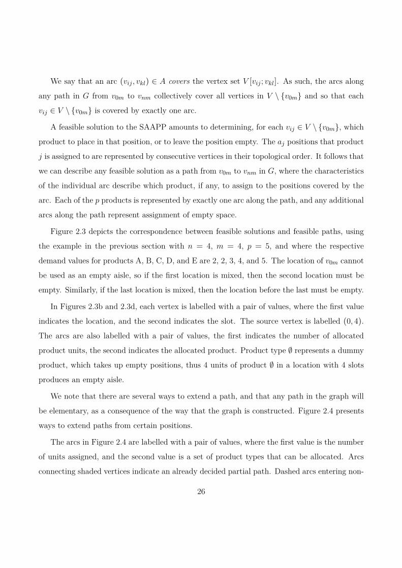
Figure 2.3 depicts the correspondence between feasible solutions and feasible paths, using
the example in the previous section with n = 4, m = 4, p = 5, and where the respective
demand values for products A, B, C, D, and E are 2, 2, 3, 4, and 5. The location of v0m cannot
be used as an empty aisle, so if the first location is mixed, then the second location must be
empty. Similarly, if the last location is mixed, then the location before the last must be empty.
In Figures 2.3b and 2.3d, each vertex is labelled with a pair of values, where the first value
indicates the location, and the second indicates the slot. The source vertex is labelled (0, 4).
The arcs are also labelled with a pair of values, the first indicates the number of allocated
product units, the second indicates the allocated product. Product type ∅ represents a dummy
product, which takes up empty positions, thus 4 units of product ∅ in a location with 4 slots
produces an empty aisle.
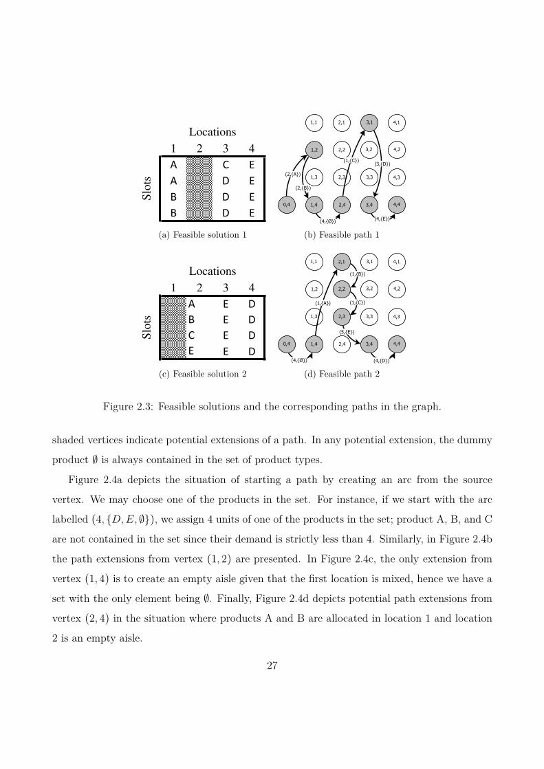
We note that there are several ways to extend a path, and that any path in the graph will
be elementary, as a consequence of the way that the graph is constructed. Figure 2.4 presents
ways to extend paths from certain positions.
The arcs in Figure 2.4 are labelled with a pair of values, where the first value is the number
of units assigned, and the second value is a set of product types that can be allocated. Arcs
connecting shaded vertices indicate an already decided partial path. Dashed arcs entering non-
26
1 2 3 4
A C E
A D E
B D E
B D E
Locations
Slo
ts
(a) Feasible solution 1 (b) Feasible path 1
1 2 3 4
A E D
B E D
C E D
E E D
Locations
Slo
ts
(c) Feasible solution 2 (d) Feasible path 2
Figure 2.3: Feasible solutions and the corresponding paths in the graph.
shaded vertices indicate potential extensions of a path. In any potential extension, the dummy
product ∅ is always contained in the set of product types.
Figure 2.4a depicts the situation of starting a path by creating an arc from the source
vertex. We may choose one of the products in the set. For instance, if we start with the arc
labelled (4, D,E, ∅), we assign 4 units of one of the products in the set; product A, B, and C
are not contained in the set since their demand is strictly less than 4. Similarly, in Figure 2.4b
the path extensions from vertex (1, 2) are presented. In Figure 2.4c, the only extension from
vertex (1, 4) is to create an empty aisle given that the first location is mixed, hence we have a
set with the only element being ∅. Finally, Figure 2.4d depicts potential path extensions from
vertex (2, 4) in the situation where products A and B are allocated in location 1 and location
2 is an empty aisle.
27
(a) Extending from source vertex (b) Extending from vertex (1,2)
(c) Extending from vertex (1,4) (d) Extending from vertex (2,4)
Figure 2.4: Extending a path.
We note that some path extensions do not lead to a feasible solution. In Figure 2.4d, for
instance, the extension from vertex (2, 4) by assigning 4 units of product D means that the
remaining products C and E must be assigned to the last location, which would then become
mixed. This, however, would be infeasible due to the absence of an empty aisle adjacent to the
last location.
2.3.2 Product clusters
Two allocated products with identical demands may be swapped in any feasible solution; such
an operation just amounts to choosing another permutation of products with equal demands.
In order to eliminate symmetries with respect to such permutations, we express the prod-
28
ucts and their demands in a compact way. In particular, we divide the p products into
d∗ = maxj=1,...,pdj clusters, where cluster i contains the products with demand equal to
i, for i = 1, . . . , d∗. As such, a characterization of the products is given by the vector
Γ0 = (γ10 , γ2
0 , . . . , γd∗0 ), where γi0 = | j : dj = i | for i = 1, 2, . . . , d∗. Using this representa-
tion, we do not distinguish between products in the same cluster. For example, the five products
in the example of Figure 2.2 are characterized by the vector (0,2,1,1,1) without distinguishing
between products A and B.
2.3.3 Empty/Mixed/Dedicated combinations
For any path ending at any vertex in location i, we keep information on the status of locations
i − 1 and i with respect to the possibility of mixing location i and whether or not mixing
location i implies a requirement for allocating an empty aisle at location i+ 1. We define a
location’s EMD-status as (E), (M), or (D), according to whether the location is empty, mixed,
or dedicated, respectively, and we let EMDi denote the EMD-status of any location i. While
we can combine the three possibilities for locations i and i− 1 to produce 3× 3 combinations,
it is in fact sufficient to distinguish between only five cases, for the following reason: if location
i is empty, then EMDi−1 makes no difference with respect to possible extensions of the path;
if, however, location i is not empty, then we only need to keep track of whether or not location
i− 1 is empty, as this determines whether or not a mixed location i implies that location i+ 1
needs to be empty. The resulting five cases are described below as part of a path label.
2.3.4 Path labels
For presentational convenience is it assumed in the following that, unless otherwise stated, any
path considered starts at vertex v0m.
With any path we associate a label which keeps the information needed to identify the path,
and we let vij denote the set of labels associated with paths ending at vertex vij . Each label
λ ∈ vij , associated with the path Pλ, contains the following information:
29
1. the total number of allocated product units along Pλ; this is the objective value of the
path and equals the total length of all those arcs along Pλ that represent allocation of
product units (i.e., excluding arcs representing empty positions);
2. Γλ = (γ1λ, γ2
λ, . . . , γd∗λ ) shows the number of yet unallocated products. As such, along Pλwe have allocated γi0 − γiλ products from cluster i, for i = 1, . . . , d∗;
3. Θλ is the combination of EMDi and EMDi−1 for Pλ and captures the aforementioned five
cases:
a) Θλ = (E) if location i is empty. In this case the EMD-status for location i− 1 makes
no difference;
b) Θλ = (M,MD): Location i is mixed, and location i− 1 is mixed or dedicated;
c) Θλ = (D,MD): Location i is dedicated, and location i− 1 is mixed or dedicated;
d) Θλ = (M,E): Location i is mixed, and location i− 1 is empty;
e) Θλ = (D,E): Location i is dedicated, and location i− 1 is empty.
We note that if λ ∈ vim and the corresponding location is dedicated, then cases (c) and
(e) could be merged, since the information about the previous location plays no role in
the continuation of the path. In the following we refer to Θλ as the EMD-value of Pλ.
2.4 A dynamic programming algorithm
Given that G is acyclic, all paths in G can be constructed by taking in topological order all
vertices in V \ vnm as source vertex vij and extend each path ending at vij by adding arcs
(vij , vkl) in all the ways that are relevant according to the problem characteristics. When all
vertices in V \ vnm have been used as source vertex, an optimal solution is provided by one
of the paths ending at vnm.
30

In combination with this, we have found it useful also to introduce a threshold value T as
an estimate of the optimal number of allocated units. Indeed, in the construction of paths as
sketched above we are concerned only with solutions having at least T allocated units.
Initially, T is set equal to an upper bound. In a single iteration of the path construction
there may or may not exist a solution with at least T allocated units. If one or more such
solutions exist, then the best found solution is indeed optimal and we terminate the procedure,
otherwise we decrease T and perform another iteration.
A stepwise description of the procedure is as follows.
Step 1: Create at vertex v0m a dummy label λ which represents an empty path (i.e., with
no arcs) with the following information: Γλ = Γ0 and the total number of allocated
product units is 0. The EMD-value for this empty path is artificially set equal to
Θλ = (D,E), so that if location 1 is mixed, then location 2 must be empty. This
dummy label is the only label in v0m.
Step 2: Perform steps 3–7 for all source vertices vij satisfying 0 ≤ order(vij) ≤ nm− 1, where
the vertices are selected in increasing order of order(vij). Finally, go to step 8.
Step 3: For each pair of labels λ, λ′ ∈ vij , detect whether λ dominates λ′ using the dominance
rule. Remove from vij any label as soon as it is found to be dominated.
Step 4: Select labels λ ∈ vij in non-increasing order of the total number of allocated product
units. For each label λ perform steps 5–7.
Step 5: Perform a feasibility verification of the given λ. If infeasibility is detected, then return
to step 4.
Step 6: Compute an upper bound (UB) for the given λ. If UB < T , then return to step 4.
Step 7: Create a set of successors S(λ) of λ as described hereinafter.
31
Step 8: If there exists at least one label in vnm, then identify in vnm a label with the maximum
value of allocated product units; this provides us with an optimal solution. Otherwise,
if there are no labels in vnm, then we can conclude that the optimal solution contains
less than T allocated units, hence we reduce T by one and return to step 2.
2.4.1 Label elimination
We have developed a number of procedures which allow us to eliminate certain labels as our
algorithm proceeds. These procedures are described in the following.
A dominance rule. We have derived the following set of conditions for detecting, for a
given label set vij and a given pair of labels λ, λ′ ∈ vij whether λ dominates λ′:
1. The total number of allocated product units of λ must be greater than or equal to that
of λ′.
2. The number of remaining products must be the same for the two labels, i.e.,
d∗∑i=1
γiλ =d∗∑i=1
γiλ′
3. Assume that condition 2 is satisfied, and let r = ∑d∗i=1 γ
iλ denote the number of remaining
products. Moreover, let (d[1]λ , . . . , d[r]λ ) be the r demands in Γλ sorted in non-increasing
order, and similarly let (d[1]λ′ , . . . , d[r]λ′ ) be the r demands in Γλ′ sorted in non-increasing
order. Then condition 3 is the following: d[i]λ ≥ d[i]λ′ for i = 1, . . . , r. The reason is that
for any choice of quantities in the completion of λ′ we can choose the same quantities in
the completion of λ by choosing the product with demand d[i]λ in the extension of Pλ as
a replacement of the product with demand d[i]λ′ in the extension of Pλ′ . Furthermore, if
d[i]λ > d
[i]λ′ for one or more values of i, then the completion of λ may lead to a strictly
better solution.
32
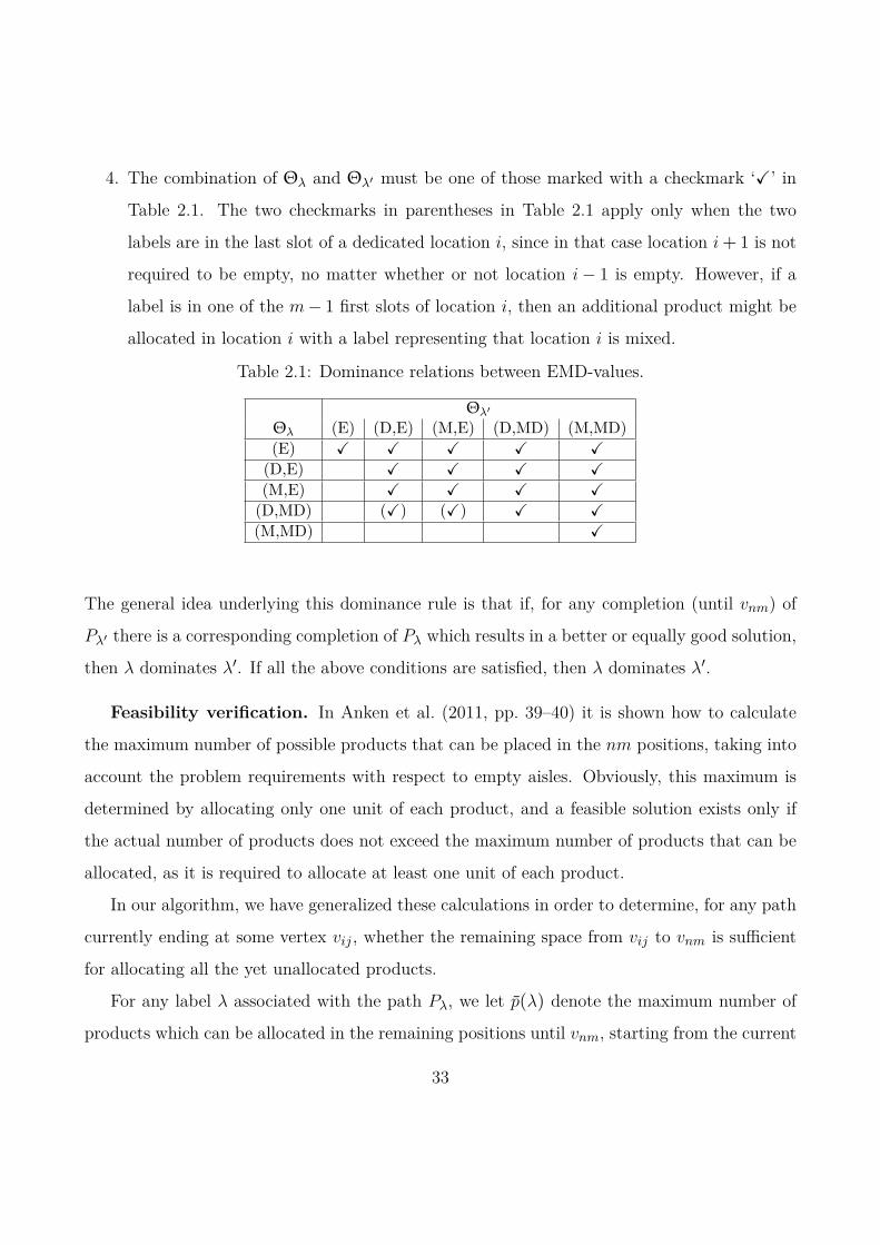
4. The combination of Θλ and Θλ′ must be one of those marked with a checkmark ‘X’ in
Table 2.1. The two checkmarks in parentheses in Table 2.1 apply only when the two
labels are in the last slot of a dedicated location i, since in that case location i+ 1 is not
required to be empty, no matter whether or not location i− 1 is empty. However, if a
label is in one of the m− 1 first slots of location i, then an additional product might be
allocated in location i with a label representing that location i is mixed.
Table 2.1: Dominance relations between EMD-values.
Θλ′
Θλ (E) (D,E) (M,E) (D,MD) (M,MD)(E) X X X X X
(D,E) X X X X(M,E) X X X X(D,MD) (X) (X) X X(M,MD) X
The general idea underlying this dominance rule is that if, for any completion (until vnm) of
Pλ′ there is a corresponding completion of Pλ which results in a better or equally good solution,
then λ dominates λ′. If all the above conditions are satisfied, then λ dominates λ′.
Feasibility verification. In Anken et al. (2011, pp. 39–40) it is shown how to calculate
the maximum number of possible products that can be placed in the nm positions, taking into
account the problem requirements with respect to empty aisles. Obviously, this maximum is
determined by allocating only one unit of each product, and a feasible solution exists only if
the actual number of products does not exceed the maximum number of products that can be
allocated, as it is required to allocate at least one unit of each product.
In our algorithm, we have generalized these calculations in order to determine, for any path
currently ending at some vertex vij , whether the remaining space from vij to vnm is sufficient
for allocating all the yet unallocated products.
For any label λ associated with the path Pλ, we let p(λ) denote the maximum number of
products which can be allocated in the remaining positions until vnm, starting from the current
33
end vertex vij of the path Pλ. Any label λ along a feasible path must satisfy ∑d∗i=1 γ
iλ ≤ p(λ),
so otherwise label λ can be discarded. Our computations of p(λ) follow the general idea in
Anken et al. (2011).
Upper bounds. For any path Pλ to vij we compute an upper bound UB on the final
number of allocations that may be obtained at vnm by extending Pλ. This bound is the sum
of two terms, namely the number of allocations made along the path until vij , and an upper
bound aλ on the remaining allocations that can be made from vij to vnm. The following are
involved in the computation of aλ:
1. The remaining number of available positions nm− order(vij) is surely a valid value of aλ.
2. The number of yet unallocated product units (∑d∗i=1 iγ
iλ) is also a valid value of aλ.
3. If Θλ = (M,MD) ∨Θλ = (D,MD), then any extension of Pλ will involve that either the
following location must be an empty aisle (i.e., if we assign further products to the current
location which then will be mixed), producing m empty positions, or the remaining m− j
positions in the current location are left empty. Together, this implies at leastm− j empty
positions on the path from vij to vnm.
4. The set of products with demands less thanm implies a certain amount of empty positions
to be allocated. A product j with dj < m will produce m − dj empty positions if
it is assigned to a dedicated location, and otherwise it must be assigned to a mixed
location which will generate a requirement for an empty aisle. We consider collectively
all the ∑m−1i=1 γiλ yet unassigned products with demands smaller than m. For a fixed
number of empty aisles we can determine a lower bound on the implied number of empty
positions by assigning up to 2m products on the two sides of each aisle—where we choose
the products in nondecreasing order of demand—and assign the remaining products to
dedicated locations; this produces m empty positions for each empty aisle plus the sum of
the m− dj values over all products j assigned to dedicated locations; we recall that only
34
products with demand smaller than m are considered. We obtain a sequence of lower
bounds by considering the case with 0, 1, 2, . . . etc. empty aisles, and finally we choose
the lower bound with the minimum number of empty positions.
Further details are omitted for the sake of brevity. If the computed upper bound UB < T , then
we can discard label λ.
Iterative probing. When determining the value of the threshold level T , we first compute
an upper bound UB on the final number of allocations based on the dummy label λ at vertex
v0m and set T = UB. As described earlier, if one or more solutions exist with at least T allocated
units, then we terminate the procedure, otherwise we decrease T and perform another iteration.
There are several alternative methods for updating T . We have chosen to use a simple method
of decreasing T by a constant amount after each iteration until an optimal solution is found. In
fact, we have chosen to decrease T by only one unit after each iteration, as we have experienced
that a T value below the optimal number of allocated units can significantly increase the total
computation time.
2.4.2 Extending a path
Given a label λ representing a path from v0m to vij , we produce the set of successor labels S(λ)
of λ by adding arcs (vij , vkl) ∈ A.
For each q = 1, . . . , d∗ we consider the possibility of extending the path by adding an arc
(vij , vkl) which represents an allocation of the quantity q. A straightforward implementation
would be to extend the path from vij with an arc for each cluster i ≥ q for which γiλ > 0.
However, we observe that for any choice of q it suffices to consider only one cluster by choosing
the smallest among sufficient demands. Formally, we let ρ(q,λ) denote the cluster from which
we choose the product to allocate, given that q units must be allocated starting from label λ,
and we determine the cluster by setting ρ(q,λ) = mini|i ≥ q ∧ γiλ > 0. Any other choice of
35

cluster for the given value of q would lead to a dominated label according to condition 3 of the
dominance rule.
In addition to allocating units of a product, we also have the possibility of allocating empty
positions. We consider these two alternatives further in the following, where we also describe
the other ingredients involved in extending a path.
Allocating empty positions. Without loss of generality we use the convention that
empty positions within a location are placed at the highest-indexed slots in the location. As
such, any arc representing empty positions ends at slot m. If the arc completes the current
location, then it is of the form (vij , vim), otherwise it is used for creating an empty aisle and is
of the form (vim, vi+1,m).
Allocation of q ∈ [m+ 1; 2m− 1] uses two arcs by first completing the current location and
then creating an empty aisle. Allocation of 2m or more empty positions in one step does not
occur; however, adjacent empty aisles can be produced by repeatedly creating single aisles.
Allocating product units. Given a product and a quantity q to be allocated, we allocate
the product to the q positions in V [vij ; vkl]. So, in general, the arc representing the allocation
of q units is directed from vij to vkl so that q = (k− i)m+ l− j. With respect to feasibility, it is
required to use the smallest possible number of locations for storing the q units. In terms of our
allocation procedure this requirement amounts to ensuring that if i < k, then the total quantity
of the product which is allocated to locations i and k exceeds m, otherwise the quantity at
location i could be moved to location k, resulting in one less location for storing the product.
This can be expressed by the restriction that l > j whenever (i < k) ∧ (j < m). However,
there is no restriction when j = m, as in that case we do not allocate any units of the product
in location i.
Ensuring feasibility with respect to mixed locations and aisles. Any mixed location
must be adjacent to an empty aisle. For satisfying this requirement we make use of the EMD-
value for the label λ that we are extending by the arc (vij , vkl), resulting in label µ at vertex
36
vkl.
In the following we distinguish between whether or not we extend from the last slot (i.e.,
j = m) in a location. It is noted that these two cases have quite different possibilities with
respect to feasibility. The details are as follows.
1. Suppose that j = m, i.e., we extend from the last slot in location i. Note that only in
this case is it possible to have Θλ = (E). We distinguish between two situations:
a) Θλ = (M,MD): Location i is mixed and must be adjacent to an empty aisle. Since
the previous location is not an empty aisle, there is only one feasible extension,
namely to allocate an empty aisle at location i+ 1. The resulting label has Θµ = (E).
b) Θλ 6= (M,MD): There are no restrictions on the extensions in any of these four cases,
so we consider all values q = 1, . . . , d∗ as the quantity for the next allocation. For
each value of q, the extension produces the first allocated product in the resulting
location k, which then becomes dedicated. The resulting label has Θµ = (D,E) if
(Θλ = (E)) ∧ (k = i+ 1), otherwise Θµ = (D,MD). Note that this also covers
all possibilities where q > m resulting in k > i+ 1. Finally, we also consider the
possibility of creating an empty aisle at location i+ 1, producing Θµ = (E).
2. Suppose that j < m. This means that we have already assigned at least one product
to location i, so Θλ 6= (E). For any of the four possible values of Θλ we may fill the
current location by adding m− j empty positions, which will produce the label Θµ = Θλ
at vertex vim. Alternatively, if we extend the path by allocating product units, then
location i will be mixed in the new label, and we distinguish between the following two
situations:
a) Θλ = (M,MD)∨Θλ = (D,MD): The previous location is not empty, so the fact that
the current location is mixed after this allocation means that the next location must
be empty. Therefore, the quantity that we allocate must not exceed the remaining
37
space in the current location, i.e., we consider only quantities q = 1, . . . , minm−
j, d∗ to be allocated. The resulting label has Θµ = (M,MD).
b) Θλ = (M,E)∨Θλ = (D,E): The previous location is empty, so the current location
can be mixed without requiring the next location to be empty. Consequently, we
consider all quantities q = 1, . . . , d∗ to be allocated, subject to the restriction that
if k > i, i.e., if we allocate more than m− j units, then it must hold that l > j in
order to use the smallest possible number of locations for the q units. Concerning
the resulting label, we note that for q ≤ m− j, we obtain Θµ = (M,E), as the
allocation is kept within the current location. For q > m− j (implying k > i) the
resulting label is Θµ = (D,MD).
2.5 Computational experiments
Computational experiments were carried out on a personal computer P8700 (2.53 GHz) with 4
GB of RAM running Windows 7. Algorithms were implemented in C with Visual Studio 10.0.
We have implemented and analyzed the following approaches: our exact algorithm Saapp,
the Cplex 12.4 implementation (Anken et al., 2011, the model of), and in addition we also
analyzed the Saapp algorithm with an initial threshold value T set to the optimal value, so
the algorithm finds an optimal solution in a single iteration. The latter setup is denoted as
Saapp/si and shows the computation time spent in the last iteration, i.e., the time needed to
prove optimality of a solution.
We have tested the performance of our algorithm by generating SAAPP instances as pro-
posed by Anken et al. (2011, p. 9). Accordingly, the number of products is in the range
[0.9n, . . . , 1.3n]. A CPU time limit of one hour was set for both the Saapp algorithm and the
Cplex implementation.
Table 2.2 presents our computational results. Each line represents average results for prob-
lems with p = 0.9n, 1.0n, 1.1n, and 1.3n. For each value of p a total of 10 problem instances
38
were tested.
The two columns under the ‘No. of replenishments’ heading show the average number of
replenishments of the instances that are solved by Cplex and Saapp, respectively, within the
CPU time limit. The number of replenishments can be automatically translated into wasted
time in the picking area (Anken et al., 2011) and is computed by taking the total demand
over the period and deducting from it the total number of allocated product units during the
advanced replenishment. The actual number of solved instances is presented under the ‘No. of
solved instances’ heading. The three columns under the ‘CPU time (sec)’ heading show the
time required by Cplex, Saapp and Saapp/si to provide an optimal solution, averaged over
the solved instances. To facilitate the comparison, Saapp/si is applied only to those instances
that are solved by Saapp within the CPU time limit.
Clearly, with respect to computing time Saapp outperforms Cplex when the number of
locations is greater than 15. In addition, the results show that Saapp can solve problems of
moderate size. Moreover, the parameter with the highest impact on the computation time is
the number of slots.
The difference in computing time between Saapp and Saapp/si shows the time spent on
iterations before we reach the T value that equals the optimal objective value. We consider
this difference as the potential saving in computation time that might be obtained by more
advanced schemes for initializing and updating the T value. We consider the time difference
between Saapp and Saapp/si to be relatively modest, hence the iterative probing seems to
be an appropriate approach for the SAAPP.
Finally, Table 2.3 presents the average number of allocated units in the optimal solution
obtained with our Saapp algorithm. Each value is the average result over 10 instances with the
specified n, m and p configuration. If we consider the effect, in terms of the number of allocated
units, of increasing either n or m by one, then the parameter with the highest impact per unit
change seems to be the number of slots, within the problem sizes that have been investigated.
Indeed, a unit increase of m increases the capacity of the flow rack by n slots. Hence, if more
39
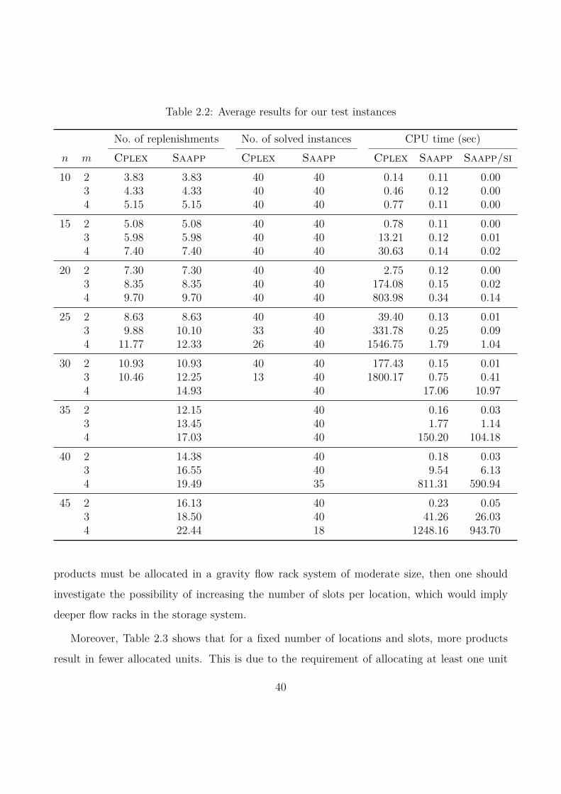
Table 2.2: Average results for our test instances
No. of replenishments No. of solved instances CPU time (sec)n m Cplex Saapp Cplex Saapp Cplex Saapp Saapp/si10 2 3.83 3.83 40 40 0.14 0.11 0.00
3 4.33 4.33 40 40 0.46 0.12 0.004 5.15 5.15 40 40 0.77 0.11 0.00
15 2 5.08 5.08 40 40 0.78 0.11 0.003 5.98 5.98 40 40 13.21 0.12 0.014 7.40 7.40 40 40 30.63 0.14 0.02
20 2 7.30 7.30 40 40 2.75 0.12 0.003 8.35 8.35 40 40 174.08 0.15 0.024 9.70 9.70 40 40 803.98 0.34 0.14
25 2 8.63 8.63 40 40 39.40 0.13 0.013 9.88 10.10 33 40 331.78 0.25 0.094 11.77 12.33 26 40 1546.75 1.79 1.04
30 2 10.93 10.93 40 40 177.43 0.15 0.013 10.46 12.25 13 40 1800.17 0.75 0.414 14.93 40 17.06 10.97
35 2 12.15 40 0.16 0.033 13.45 40 1.77 1.144 17.03 40 150.20 104.18
40 2 14.38 40 0.18 0.033 16.55 40 9.54 6.134 19.49 35 811.31 590.94
45 2 16.13 40 0.23 0.053 18.50 40 41.26 26.034 22.44 18 1248.16 943.70
products must be allocated in a gravity flow rack system of moderate size, then one should
investigate the possibility of increasing the number of slots per location, which would imply
deeper flow racks in the storage system.
Moreover, Table 2.3 shows that for a fixed number of locations and slots, more products
result in fewer allocated units. This is due to the requirement of allocating at least one unit
40

per product. Specifically, more products tend to produce more mixed locations which in turn
increase the number of empty aisles, leaving less space for allocation of products.
Table 2.3: Average number of allocated units with Saapp
(a) p = 0.8n
nm 15 20 25 30 35 avg2 26.80 35.40 44.50 53.40 62.90 44.603 40.30 53.30 67.00 80.10 94.50 67.044 53.90 71.90 89.90 107.80 125.30 89.76avg 40.33 53.53 67.13 80.43 94.23
(b) p = 1.0n
nm 15 20 25 30 35 avg2 25.90 34.00 43.10 51.20 60.40 42.923 39.10 52.20 65.50 79.10 92.30 65.644 53.10 71.00 88.70 105.70 124.00 88.50avg 39.37 52.40 65.77 78.67 92.23
(c) p = 1.1n
nm 15 20 25 30 35 avg2 25.00 33.40 41.90 49.70 58.10 41.623 38.90 51.00 64.70 76.70 91.30 64.524 52.60 70.40 87.70 104.80 122.40 87.58avg 38.83 51.60 64.77 77.07 90.60
(d) p = 1.3n
nm 15 20 25 30 35 avg2 22.00 28.00 36.00 42.00 50.00 35.603 37.80 50.10 62.40 75.10 88.10 62.704 50.80 67.90 84.40 102.00 120.20 85.06avg 36.87 48.67 60.93 73.03 86.10
Based on the results with the set of generated problem instances, we conclude that the
41
exact Saapp algorithm can be applied to obtain optimal solutions of moderate size instances.
2.6 Conclusions
In this paper, we have presented an exact dynamic programming algorithm for the space allo-
cation and aisle positioning problem (SAAPP) which deals with two important and interrelated
problems, namely, the product allocation problem and the storage location assignment problem.
To the best of our knowledge, this is the first exact algorithm for the SAAPP. We have
introduced an appropriately defined graph representation of the SAAPP, which explores the
characteristics of the underlying problem structure and enables the development of the dynamic
programming algorithm.
Indeed, our computational study performed on numerous data shows that our exact algo-
rithm can be used to find optimal solutions to SAAPP instances of moderate size.
42

Chapter 3
Scheduling in a Cross-Dock Environment to
Minimize Mean Completion Time

Scheduling in a Cross-Dock Environmentto Minimize Mean Completion Time
Peter Bodnar and Jens Lysgaard
CORAL, Department of Economics and Business, Aarhus University, Denmark
[email protected] and [email protected]
Abstract
This paper studies the problem of minimizing the mean completion time of outbound
trucks in a cross-dock environment with a single inbound door and a single outbound door.
Minimizing mean completion time improves the cross-dock’s responsiveness and is known
to lead to stable or balanced utilization of resources, rapid turn-around of vehicles and
reduction of in-process inventory. We address the problem from a flow shop scheduling
perspective and exploit its similarities with the classical two-machine flow shop problem,
i.e., F2||∑
Cj . Indeed, our problem is a generalization of F2||∑
Cj , which is known
to be NP-hard. We propose a branch-and-bound algorithm to find an optimal solution
to the problem. Computational results show that our branch-and-bound algorithm can
optimally solve problem instances of moderate size within a reasonable amount of time.
3.1 Introduction
Cross-docks are facilities in which inbound vehicles deliver products that are rapidly distributed,
consolidated, and transferred to outbound vehicles. Cross-docks aim to minimize or even elim-
44
inate the cost of storing and retrieving products. Products are either transferred from inbound
to outbound vehicles or placed in a buffer area for a short period, typically less than 24 hours.
Moreover, cross-docking can reduce transportation costs by enabling higher capacity utiliza-
tion for inbound and outbound vehicles. Cross-docking has been successfully implemented in
several industries such as at retail chains (Stalk et al., 1992), mailing companies (Forger, 1995),
automobile manufacturers (Witt, 1998), and less-than-truckload logistics providers (Gue, 1999).
The literature on cross-docking is mainly focused on truck scheduling and truck-to-dock
assignment problems. For recent comprehensive literature reviews we refer to Agustina et al.
(2010), Boysen and Fliedner (2010), and Van Belle et al. (2012). Truck-to-dock assignment is
the problem of assigning inbound and outbound trucks to docks (Tsui and Chang, 1990, 1992;
Oh et al., 2006; Miao et al., 2009). Note that the truck-to-dock assignment problem is different
from the truck scheduling problem, which takes time dimension into account while time is not
considered in the dock door assignment problem (Konur and Golias, 2013).
In the existing literature on truck scheduling problems in cross-docking, optimization criteria
are typically based on completion times of the vehicles. The most common and widely studied
performance measure of cross-dock operations is the makespan, defined as the completion time
of the last outbound vehicle (Yu and Egbelu, 2008; Chen and Song, 2009; Chen and Lee, 2009;
Boysen et al., 2010). This objective is appropriate when the cost of a schedule depends on how
long the processing system is devoted to the entire set of vehicles. Moreover, the makespan
is known to be directly related to the maximization of the throughput and the usage of the
resources, e.g., dock doors.
In this research we focus on individual outbound trucks and minimize the mean completion
time, which is equivalent to minimizing the total completion time defined as the sum of the
completion times of the outbound trucks. The objective is also referred to as the total flow
time if all trucks are available from the beginning of the planning horizon. This performance
measure improves the cross-dock’s responsiveness and leads to stable or balanced utilization
of resources, rapid turn-around of vehicles, and reduction of in-process inventory (Rajendran
45
and Ziegler, 1997; Framinan and Leisten, 2003). Therefore, it is considered to be relevant and
meaningful for today’s dynamic production environment (Liu and Reeves, 2001).
This objective criterion has been recently addressed by Briskorn et al. (2013) and Soltani and
Sadjadi (2010). Briskorn et al. (2013) consider the problem of minimizing the total weighted
completion time in a single dock cross-docking facility with inventory constraints. The authors
show that the problem is NP-hard and propose a branch-and-bound and a dynamic program-
ming algorithm. Soltani and Sadjadi (2010) assume a single inbound and a single outbound
dock system with no temporary storage and develop two robust hybrid meta-heuristic methods.
We extend the literature by focusing on minimizing the total completion time of outbound
trucks in a single inbound and single outbound door cross-dock environment with temporary
storage and propose an exact branch-and-bound approach.
The structure of this paper is the following. In Section 3.2 we describe the problem and
provide an illustrative example. The properties of the problem are presented in Section 3.3. In
Section 3.4 we describe lower bound procedures which can be embedded in a branch-and-bound
framework as presented in Section 3.5. Results of the computational experiments are reported
in Section 3.6. Finally, conclusions are presented in Section 3.7.
3.2 Problem description
We consider a cross-dock with a single inbound and a single outbound dock door. We assume
complete information about the inbound and outbound vehicles. Each inbound truck may carry
several products to a set of outbound trucks, and each outbound truck may receive products
from several inbound trucks. We assume a pre-distribution system, which is applied frequently
in practice (Yan and Tang, 2009), i.e., each incoming product is assigned to a single outbound
truck prior to the product’s arrival at the cross-dock, hence each product can be considered
as a unique product type and a transshipment matrix can completely describe the predecessor
relations between trucks.
46

Moreover, each truck is available from the beginning of the planning horizon and associated
with a known processing time. Processing (i.e., loading) of an outbound truck cannot be
initiated before all its associated products have been unloaded from their respective inbound
trucks and the outbound dock has become idle. We assume that the transshipment time of
products in the cross-dock is negligible (i.e., we assume that it is zero) when searching for
a solution. Finally, storage capacity is assumed to be unlimited and sufficient workforce is
assumed to be available in the cross-dock to process the trucks.
Cross-dock scheduling is closely related to traditional machine scheduling (Chen and Lee,
2009; Briskorn et al., 2013). However, cross-dock scheduling involves some peculiarities, for
which classical machine scheduling approaches or even notation cannot be used directly, e.g., in
a cross-dock inbound vehicles might contain multiple product units, which are not preassigned
to a specific vehicle but may satisfy the demand of multiple outbound vehicles for the respective
product (Boysen and Fliedner, 2010).
We formulate the problem as a two-machine flow shop problem and consider two sets of jobs
with precedence constraints. The job sets correspond to inbound and outbound vehicles while
the two machines correspond to a single inbound and a single outbound dock, respectively.
For notational convenience, when referring to a problem we follow the 3-field notation
[α|β|γ] for cross-docking scheduling problems introduced by Boysen and Fliedner (2010), where
α is door environment, β is the operational characteristics, and γ is the objective. The notation
uses square brackets in order to clearly distinguish the considered cross-docking problem from
problems in a classical scheduling environment. Accordingly, our problem can be denoted as
[E2|tλ=0|∑Cj ] and stated as the following.
47

[E2|tλ=0|∑Cj ] Problem: There are two machines M1 and M2 and two set of jobs
I = i1, i2, . . . , in and O = o1, o2, . . . , om. Each job j ∈ I must be processed on
M1 and requires a processing time of a(j). Each job j ∈ O must be processed on M2
and requires a processing time of b(j). For each job j ∈ O, there is a corresponding
predecessor set Pj of jobs in I, such that all jobs in Pj must be completed on M1
before j can be processed on M2. We aim to schedule jobs in I and O, such that the
total completion time of jobs in O, i.e., the sum of the m completion times on M2, is
minimized.
The problem addressed in this paper can be considered as a generalized two-machine flow
shop problem, which is a common problem in production environments where the two machines
represent two processing stages that products must visit in order. In particular, a special case
of our problem, when a single inbound truck serves a single outbound truck, is equivalent to
the two-machine minimum total completion time flow shop problem. We follow the notation
by Graham et al. (1979) and use F2||∑Cj to denote this classical problem. We note that
in F2||∑Cj the transshipment time of the jobs between the first and second machine is also
ignored, i.e., assumed to be zero. The F2||∑Cj is known to be NP-hard in the strong sense
(Gonzalez and Sahni, 1978; Framinan and Leisten, 2003), therefore, [E2|tλ=0|∑Cj ] is also
NP-hard.
Furthermore, we use the following notation throughout the paper:
Si is the successor set of job i ∈ I, Si ⊆ O, i.e., o ∈ Si if and only if i ∈ Poπ is a sequence of jobs in I processed on M1,
π = (π1, π2, . . . , πl) with l ≤ n, i.e., πk is the kth element of π
σ is a sequence of jobs in O processed on M2,
σ = (σ1,σ2, . . . ,σl) with l ≤ m, i.e., σk is the kth element of σ,
σ is a complete sequence of jobs in I if l = m,
otherwise it is a partial sequence
σ is the complement set of a sequence σ, i.e., σ = O \ σ
48

Ω is a schedule that corresponds to a tuple (π,σ)
C(j) is the completion time of job j ∈ I,O
Ci(Ω) is the completion time of the last job on Mi according to Ω
[E2|tλ=0|∑Cj ] can be formulated as follows:
min∑o∈O
C(o) (3.1)
subject to
C(i)− a(i) ≥ 0 ∀i ∈ I (3.2)
C(o)− b(o) ≥ C(i) ∀o ∈ O, i ∈ Po (3.3)
C(i)− a(i) ≥ C(i′) ∨ C(i′)− a(i′) ≥ C(i) ∀i, i′ ∈ I, i 6= i′ (3.4)
C(o)− b(o) ≥ C(o′) ∨ C(o′)− b(o′) ≥ C(o) ∀o, o′ ∈ O, o 6= o′ (3.5)
The objective function (3.1) aims to minimize the total completion time. Constraints (3.2)
ensure that the processing of any job onM1 does not start before the beginning of the planning
horizon. Constraints (3.3) ensure that the processing of any job onM2 can commence only after
all its predecessors are completed onM1. Constraints (3.4)–(3.5) ensure that each machine can
process at most one job at a time.
Consider an example with 6 inbound and 4 outbound trucks, i.e., I = i1, i2, . . . , i6 and
O = o1, o2, o3, o4. The predecessor relations and processing times are given in Table 3.2. A
feasible schedule is presented in Figure 3.1, for this instance this is also an optimal schedule
with a total completion time of 110, i.e., a mean completion time of 27.5. That is, an optimal
solution to this problem is the following: π = (i2, i4, i5, i3, i6, i1) and σ = (o1, o2, o3, o4).
49

Table 3.2: Example
(a) Jobs in I
Job i1 i2 i3 i4 i5 i6
a(j) 6 5 8 4 4 6Sj o4 o1, o4 o3, o4 o1, o2 o2, o4 o3
(b) Jobs in O
Job o1 o2 o3 o4
b(j) 5 10 4 8Pj i2, i4 i4, i5 i2, i3, i5, i6 i1, i2, i3
M1 i2 i4 i5 i3 i6 i1
M2 o1 o2 o3 o4
0 5 10 15 20 25 30 35 40
0 5 10 15 20 25 30 35 40
Figure 3.1: Representation of a schedule (arrows represent predecessor relations)
3.3 Optimality properties
Jobs in I can be scheduled consecutively on M1 without slack (or idle time) between any two
jobs, since no job in I has a predecessor. Therefore, a sequence of jobs in I and their respective
processing times provide complete information about the schedule on M1, namely starting and
completion times of each job in I.
There is a feasible solution for any given sequence of jobs in I, since one can always schedule
jobs in O in an arbitrary order after the completion time of the last job on M1.
The following property is useful for sequencing jobs in I without successors.
Property 1. There exists an optimal schedule such that job i ∈ I with Si = ∅ is sequenced
after any i′ ∈ I with Si′ 6= ∅.
Proof. Assume that some job i ∈ I with Si = ∅ is sequenced immediately before some other
50
job i′ ∈ I with Si′ 6= ∅. When exchanging these two jobs, i, i′ on M1, no job is delayed on M2.
Therefore, applying such exchanges iteratively, any job i ∈ I with Si = ∅ can be sequenced
after any i′ ∈ I with Si′ 6= ∅ without delaying the completion time of any job on M2.
Moreover, any job i ∈ I with Si = ∅ that is sequenced last on M1 can be removed from a
solution, since the quality of the solution is measured only by considering completion times on
M2. Therefore, from now on, we assume that Si 6= ∅ for all i ∈ I.
Just as there exists a feasible solution for any given sequence of jobs in I, there exists also a
feasible solution for any given sequence of jobs in O (cf. Chen and Lee, 2009, on the makespan
minimization problem). In particular, for a given sequence σ of jobs in O, one can create a
sequence of jobs on M1 according to the order in which their successors are processed on M2,
i.e., by first sequencing jobs in Pσ1 , then jobs in Pσ2 \ Pσ1 , then iteratively sequencing jobs
in Pσj \(∪j−1k=1Pσk
)for j = 3, . . . ,m. In each iteration, the jobs that are just added to the
schedule can be sequenced arbitrarily and the processing of the current j ∈ σ begins as soon as
all jobs in Pj are completed andM2 is idle. Let the stepwise-extended order of inbound jobs for
a given sequence σ ∈ O be defined as Pσ1 ,Pσ2 \ Pσ1 ,Pσ3 \ (Pσ1 ∪ Pσ2) , . . . ,Pσm \(∪m−1k=1 Pσk
).
Property 2. There exists an optimal schedule such that if jobs in O are processed on M2
according to the sequence σ, then jobs in I are processed on M1 in the stepwise-extended order.
Proof. Assume that a schedule is given and consider two jobs j, j′ ∈ σ, where σ = (o1, o2, . . . , om)
(after re-indexing) such that j is sequenced immediately before j′ onM2 and some i′ ∈ Pj′ \Pj ,
is sequenced before some i ∈ Pj on M1. The claim is that exchanging i and i′ does not increase
the total completion time of jobs in σ. Without loss of generality, assume the following partial
sequence on M1: (i′,α, i), where α is a partial sequence of jobs in π \ i, i′. We note that the
processing of j can start only after the completion of i. Therefore, exchanging i and i′, which
produces the partial sequence (i,α, i′), does not delay the completion time of j. Moreover,
such exchanging procedure does not delay the completion time of j′ either since σ is unchanged
and defines that job j′ is processed after j. After exchanging i and i′ the new solution is
51
still feasible. Repeating this exchange process, jobs on M1 will eventually be sequenced in the
stepwise-extended order as claimed.
In the following, we assume that whenever a σ is given, then jobs in ∪j∈σPj are contained
in π and sequenced on M1 in the stepwise-extended order.
Furthermore, we can establish that a set of jobs in I with each element having the same
successor set can be considered as one block. The following property states this observation
formally.
Property 3. If for some jobs i, i′ ∈ I, i 6= i′ we have that Si = Si′, then there exists an
optimal schedule such that i and i′ are processed consecutively on M1.
Proof. Assume that two jobs i, i′ ∈ I with Si = Si′ are not processed consecutively on M1 and
let α be the partial sequence of jobs processed between i and i′, i.e., the partial sequence of
these jobs is (i,α, i′). Note that no job j ∈ Si can start being processed after having completed
i on M1 since any such job j also has i′ as predecessor, thus the processing of j can be started
only after i′ is completed on M1. Hence, exchanging i and any job in α does not delay any job
j ∈ Si, and the new solution is still feasible. As a conclusion, i can be exchanged with all jobs
in β resulting in the partial sequence (β, i, i′), which is at least as good as (i, β, i′) with respect
to the total completion time.
Consider two jobs i, i′ ∈ I, with Si = Si′ ; Property 3 implies that i and i′ together can
be considered as one block when scheduling the inbound trucks. Therefore, whenever two
such jobs are identified, we can reduce the size of the problem by replacing the two jobs with
a newly constructed job that represents the block, i.e., the new job represents both original
jobs (see Figure 3.2). In particular, let job clustering of two jobs i, i′ ∈ I, with Si = Si′ be
defined as constructing a new job i∗, where Si∗ := Si and a(i∗) := a(i) + a(i′), and setting
I := I \ i, i′ ∪ i∗ and Po := Po \ i, i′ ∪ i∗, ∀o ∈ Si∗ .
Corollary 1. Job clustering of two jobs i, i′ ∈ I, with Si = Si′ does not change the total
completion time of jobs on M2.
52
M1
M2
i i′
(a) Original instance
M1
M2
i∗
(b) New instance
Figure 3.2: Illustration of a job clustering (arrows represent predecessor relations)
Now, we present a set of conditions based on a lower bound procedure presented by Ignall
and Schrage (1965) for the F2||∑Cj ; a complete schedule is optimal if it satisfies all conditions
in the set.
Property 4. A complete schedule Ω = (π,σ) is optimal if all of the following conditions hold:
• jobs in O are sequenced according to the shortest processing time (SPT) rule;
• the first job in σ has the minimum total predecessor processing time, i.e.,∑i∈Pσ1
a(i) = mino∈O∑k∈Po a(k);
• M2 is not idle between processing any two jobs in σ.
Proof. Consider a relaxation of the [E2|tλ=0|∑Cj ] problem, the single machine problem with
the set O of jobs and processing times b(j) ∀j ∈ O. The optimal solution for this relaxation
can be found by sequencing jobs in O according to the SPT rule. Let σ denote such a complete
sequence of jobs in O. We note that in this schedule, the machine is not idle between any two
jobs.
In our cross-dock environment the earliest time that the processing of any job in O can
start on M2 is mino∈O∑k∈Po ak. Let r denote this minimum total predecessor processing time.
Hence, moving all jobs on M2 to the right by r time units, i.e., increasing the total completion
time with m · r, is a valid lower bound to our problem.
If we adopt σ for the [E2|tλ=0|∑Cj ] problem and in the resulting schedule M2 is not idle
between any two jobs while considering the original predecessor relations, then the objective
53

value is equal to the provided lower bound so σ is optimal also for the [E2|tλ=0|∑Cj ] problem.
With the help of this property, we can identify the following special case of our problem
which can be solved in O(m logm) time.
Corollary 2. If Pj = Pj′ for all j, j′ ∈ O, the problem is polynomially solvable by sequencing
jobs in O according to the SPT rule.
In the general case, there are n!m! feasible sequences in total. However, due to Property
2 the search space reduces to consider only outbound job sequences, i.e., O(m!) sequences.
Clearly complete enumeration is limited to the smallest instances.
3.4 Lower bounds
In this section, we present procedures that provide valid lower bounds. These procedures are
useful to evaluate the performance of a heuristic method and they can be embedded in exact
approaches such as branch-and-bound.
3.4.1 Predecessor relaxation based lower bounds
First, we build on the ideas presented by Ignall and Schrage (1965) for the F2||∑Cj in their
seminal paper. The key element is to process jobs on M2 without idle times by allowing either
that M2 can process multiple jobs simultaneously or by relaxing the predecessor processing
constraints on M1. We denote the lower bounds obtained with these approaches as LB1 and
LB2, respectively.
To apply the lower bound procedure LB1, we first construct an instance for the F2||∑Cj
problem based on the instance in question for our [E2|tλ=0|∑Cj ]. For this, we consider an
instance I of [E2|tλ=0|∑Cj ], in which there exists at least one job in I such that it has more
than one successor job in O. We aim to relax the successor relations and obtain an instance
54
in which one inbound truck serves one outbound truck, i.e., |Si| = 1 ∀i ∈ I. This is achieved
with an iterative procedure, as follows. In each iteration, a job i ∈ I is divided into a set of
newly constructed parts where the total processing time of the parts is a(i) and each part k
has a successor set Sk ⊆ Si. We then replace job i with the set of newly constructed parts.
In particular, let job splitting of a job i ∈ I be defined as a three phase procedure that
operates as follows. First, we construct a set D(i) of new jobs, where ∑k∈D(i) a(k) = a(i) and
∪k∈D(i)Sk ⊆ Si. Second, we set I := I \ i ∪ D(i) and remove i from the predecessor sets,
i.e., Pj := Pj \ i ∀j ∈ O. Finally, we update the predecessor sets, so that they contain the
elements of D(i), i.e., for all k ∈ D(i) we set Pj := Pj ∪ k ∀j ∈ Sk.
Then a new instance I ′ is constructed by modifying I such that we apply job splitting on
a job i ∈ I, with |Si| > 1. We call the new instance obtained reversible if Sk = Si for all
k ∈ D(i); otherwise it is called non-reversible. The following observation is used to establish a
valid lower bound.
Proposition 1. The total completion time of an optimal schedule for I ′ is a valid lower bound
of the total completion time for I.
Proof. We can distinguish two cases based on whether I ′ is reversible or not. We will prove
that the claim holds in both cases.
First, consider the case that I ′ is reversible. That is, Sk = Sk′ for all k, k′ ∈ D(i), which
implies that jobs in D(i) can be processed consecutively on M1 (see Property 3) and any two
jobs in D(i) can be clustered. Hence, the optimal total completion times for I and I ′ are
identical.
Second, consider the case that I ′ is non-reversible. That is, there exists some k ∈ D(i) such
that Sk ⊂ Si. Let I ′ and O′ denote the set of jobs in the instance I ′ that are processed on
M1 and M2, respectively. Since the job splitting procedure operates on the predecessor sets
but does not modify the set of jobs on M2, we have that each job in O′ corresponds to a job
in O, where O is the set of jobs in the instance I that are processed on M2. Without loss of
generality, assume that j′ ∈ O′ corresponds to j ∈ O and i ∈ Pj while k 6∈ Pj′ , where k ∈ D(i).
55
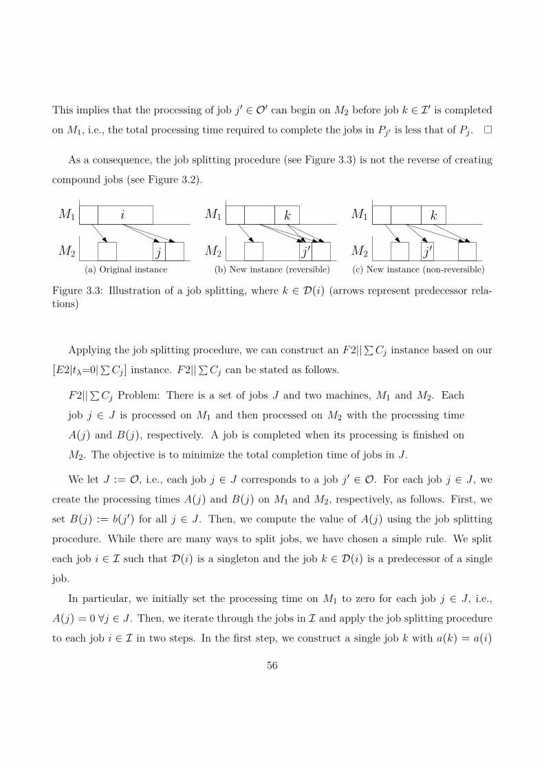
This implies that the processing of job j′ ∈ O′ can begin on M2 before job k ∈ I ′ is completed
on M1, i.e., the total processing time required to complete the jobs in Pj′ is less that of Pj .
As a consequence, the job splitting procedure (see Figure 3.3) is not the reverse of creating
compound jobs (see Figure 3.2).
M1
M2
i
j(a) Original instance
M1
M2
k
j′
(b) New instance (reversible)
M1
M2
k
j′
(c) New instance (non-reversible)
Figure 3.3: Illustration of a job splitting, where k ∈ D(i) (arrows represent predecessor rela-tions)
Applying the job splitting procedure, we can construct an F2||∑Cj instance based on our
[E2|tλ=0|∑Cj ] instance. F2||∑Cj can be stated as follows.
F2||∑Cj Problem: There is a set of jobs J and two machines, M1 and M2. Each
job j ∈ J is processed on M1 and then processed on M2 with the processing time
A(j) and B(j), respectively. A job is completed when its processing is finished on
M2. The objective is to minimize the total completion time of jobs in J .
We let J := O, i.e., each job j ∈ J corresponds to a job j′ ∈ O. For each job j ∈ J , we
create the processing times A(j) and B(j) on M1 and M2, respectively, as follows. First, we
set B(j) := b(j′) for all j ∈ J . Then, we compute the value of A(j) using the job splitting
procedure. While there are many ways to split jobs, we have chosen a simple rule. We split
each job i ∈ I such that D(i) is a singleton and the job k ∈ D(i) is a predecessor of a single
job.
In particular, we initially set the processing time on M1 to zero for each job j ∈ J , i.e.,
A(j) = 0 ∀j ∈ J . Then, we iterate through the jobs in I and apply the job splitting procedure
to each job i ∈ I in two steps. In the first step, we construct a single job k with a(k) = a(i)
56

and set D(i) := k. In the second step, the successor set Sk ⊆ Si is constructed such that it
contains a single element. For this, let Q(i) denote a set of jobs in J , such that each job j ∈ Q(i)
corresponds to a job j′ ∈ Si. We note that Si ⊆ O and Q(i) ⊆ J . We identify a job in Q(i)
with the minimum processing time onM1, let j∗ denote this job, i.e., j∗ = arg minj∈Q(i)A(j).
Then, we set the single job in Sk so that it is the job in O that corresponds to j∗. Finally, we
increase the processing time of j∗ onM1 by a(i), i.e., A(j∗) := A(j∗) + a(i), and the procedure
iteratively continues with the following job in I.
We note that the value of A(j) ∀j ∈ J can be obtained, even if some elements of the
previously described procedure are omitted. Indeed, for each i ∈ I, it is sufficient to find
j∗ ∈ J and update the processing time of j∗ on M1. The pseudo code of the procedure is
presented in Algorithm 1. It enables us to consider a starting schedule Ω = (π,σ), where σ is
a sequence of r jobs. For this, we introduce the following notation. For each i ∈ I, let Q(i)
denote a set of jobs in J , where each job j ∈ Q(i) corresponds to a job j′ ∈ Si \ σ.
Algorithm 1 Computing A(j) ∀j ∈ J
1 A(j) = 0 ∀j ∈ J2 for each i ∈ I do3 if i 6∈ Pj for all j ∈ σ then4 j∗ = arg minj∈Q(i)A(j) (break ties arbitrary)5 A(j∗) := A(j∗) + a(i)6 end if7 loop
Once A(j) and B(j) are available for all j ∈ J we can compute a lower bound as described
by Ignall and Schrage (1965), that is
LB1 =r∑j=1
C(σj) +m−r∑p=1
[C1(Ω) + (n− r− p+ 1) A(jp) +B(jp)
](3.6)
where j1, j2, . . . , jn−r is a permutation of the unscheduled jobs in J such that A(j1) ≤ A(j2) ≤
· · · ≤ A(jn−r). That is, the processing of each job can start on M2 immediately after being
57

processed onM1, irrespective of whetherM2 is idle or not. The optimal solution of this relaxed
problem is given by sequencing the jobs according to the SPT rule on M1. The complexity of
computing LB1 for a given schedule is O(m logm) at the root node and O(m) for all other
nodes (Della Croce et al., 1996).
We incorporate a further improvement to this lower bound based on a relaxation of the
problem as proposed by Della Croce et al. (1996). In particular, consider two adjacent jobs j
and j′ in J such that j is sequenced immediately before j′. In F2||∑Cj we have that j′ cannot
be processed on M2 before time maxC2(j),C1(j′), where Ci(j) is the completion time of
job j on Mi. This constraint is omitted in a relaxed problem, called F2rel||∑Cj , which has
that j′ cannot be processed on M2 before time maxC1(j) +B(j),C1(j′).
It is shown in Della Croce et al. (1996) that a lower bound to F2rel||∑Cj is given by
LBDNT1 = LB1 + Γ, where Γ is the minimum solution value over all permutations of unsched-
uled jobs in J for the expressionm−r∑p=1
[max
0,B(jp)−A(jp+1)
+ max
0,A(jp)−A(jp+1)
](3.7)
To find Γ an asymmetric traveling salesman problem based model is proposed in the paper
and a lower bound of Γ is found by a bipartite weighted matching relaxation. The complexity
of computing LBDNT1 is O(m3).
The second lower bound procedure is based on a relaxation that the processing of jobs on
M2 can start immediately after the minimum total predecessor time is completed on M1 and
M2 is idle. That is, the earliest processing time is identical for each unscheduled job in O. This
approach is equivalent to relaxing constraint (3.3) in the formulation and introducing
C(o)− b(o) ≥ mini∈IC(i) ∀o ∈ O (3.8)
The optimal solution of this relaxed problem is given by sequencing the jobs according to the
SPT rule on M2. We note that this approach is not restricted to the F2||∑Cj formulation,
therefore we may utilize the information from the [E2|tλ=0|∑Cj ] problem. In particular, we
58

use the information about the predecessor sets when selecting k in σ and call the resulting
formulation LB2. Let Ω = (π,σ) denote a starting partial schedule, we thus have that
LB2 =r∑j=1
C(σj)+m−r∑p=1
max
C2(Ω) , C1(Ω) + mink∈σ∑
i∈Pk\πa(i)
+ (n− r− p+ 1) · b(op)
(3.9)
where o1, o2, . . . , on−r is a permutation of jobs in σ such that b(o1) ≤ b(o2) ≤ · · · ≤ b(on−r).
The complexity of computing LB2 for a given σ is O(nm+m logm) at the root node and
O(m) for all other nodes.
3.4.2 A preemption based lower bound
Here, we follow the idea presented by Ahmadi and Bagchi (1990) for the F2||∑Cj and adapt
it to the cross-docking context. We therefore construct, an m-job single machine problem
instance with unequal release dates, in which the set of jobs is J := O, i.e., each job j ∈ J
corresponds to a job j′ ∈ O. Each job j ∈ J is associated with a processing time B(j) := b(j′)
and a release date
rj = max
C2(Ω),C1(Ω) +∑
i∈Pj\πa(i)
(3.10)
where Ω = (π,σ) is a starting partial schedule. The preemptive relaxation of this problem,
i.e., 1|rj , pmtn|∑Cj is efficiently solvable by applying the shortest remaining processing time
(SRPT) rule (Ahmadi and Bagchi, 1990; Chu, 1992). For this, the release dates are computed
first. Second, when a job is to be selected for processing among the available ones, the job
with the smallest remaining processing time is chosen. An arriving job preempts the job
being processed if the processing time of the new arrival is strictly smaller than the remaining
processing time of the job in process.
Let LB3 denote the solution value of an optimal solution to the 1|rj , pmtn|∑Cj . The lower
bound LB2 is dominated by LB3. However, for a given schedule, the complexity of computing
LB3 is O(nm+m logm) at the root node and O(m logm) for all other nodes.
59
3.5 Branch-and-bound
Among the exact methods, branch-and-bound algorithms have been widely applied to mini-
mization problems in which a solution is a permutation of a set of objects, particularly for
machine scheduling problems like the F2||∑Cj . A branch-and-bound algorithm is generally
characterized by a branching rule, a search strategy, node elimination rules, lower-bound cost
functions, upper-bound cost functions, and node dominance relations. We describe the details
of these elements in the following.
3.5.1 Branching rule
We adopt the branching rule presented in the paper of Ignall and Schrage (1965), in which the
authors address the F2||∑Cj problem by a branch-and-bound approach with branching on
the job to be appended to a partial sequence. The rationale for this approach is that for every
explored node corresponding to a partial sequence σ the completion times on both machines
are already computed and hence a new partial sequence constructed by appending a job to the
partial sequence can be evaluated in a few, simple steps (T’kindt et al., 2004).
A diagram representing the branch-and-bound process is called a search tree. In this tree,
each node represents a sub-problem with a given fixed partial sequence of jobs, that is, we
branch on the successive job j ∈ O to be inserted in the sequence. In particular, the kth level
of the search tree corresponds to a partial sequence with k elements.
3.5.2 Search strategy
To decide which node to branch from in the search tree, we consider the best first, the breadth
first and the depth first search strategies. It is known that the first two mentioned strategies
may require significantly more storage space when compared to last one. When the number
of generated nodes is a key element, as in our problem, depth first is generally considered the
most efficient search strategy (T’kindt et al., 2004). We therefore apply this strategy and select
60

the active node at the lowest level in the tree, namely the node with the largest number of
sequenced jobs, i.e., we explore along each branch of the search tree as far as possible before
backtracking.
3.5.3 Elimination rules
For each sub-problem of the search tree a lower bound is computed. In order to adopt the
tightest lower bound, we choose the maximum of the computed values as the lower bound to
be used for pruning branches:
LB = maxLBDNT1 ,LB2,LB3 (3.11)
If the lower bound of a given node is greater than or equal to the current upper bound (UB)
in our minimization problem, then the node is pruned.
3.5.4 Upper bounds
At the beginning of the search we establish an initial UB by applying heuristic procedures.
Moreover, we can improve on this UB during the search by evaluating complete sequences of
jobs in O, which are created during the execution of the lower bound procedures.
Initial upper bound
Several heuristic procedures have been proposed for the F2||∑Cj problem. These often follow
a general framework composed of three phases, namely job indexing, solution construction,
and solution improvement (Framinan et al., 2005; Pan and Ruiz, 2013). Framinan et al. (2005)
cluster the existing heuristics into two groups: simple and composite methods. A heuristic is
called composite if it employs another heuristic for one or more of the three phases. Otherwise
the procedure can be categorized as a simple heuristic.
61

The solution to the problem can be described by the job schedule on M2 alone since it
defines the job schedule on M1 as well. Therefore, the heuristic procedures are focused on a
sequence of jobs on M2.
We have implemented a simple heuristic, the procedure of Laha and Sarin (2009), called
FL-LS, which is considered the best performer among simple heuristics (Pan and Ruiz, 2013)
and runs in O(m4) time, where m is the number of jobs in O. The procedure is outlined in
the following.
Step 1: Compute Tj , the total processing time on both machines for each job j ∈ O, i.e.,
Tj =∑i∈Pj
a(i) + b(j) ∀j ∈ O (3.12)
Step 2: Sort jobs in O in non-decreasing order of their total processing times.
Step 3: Set k = 1 and construct a partial sequence with the first job from the sorted list.
Step 4: Update k := k + 1. Select the kth job from the list and insert it into the best of the
k possible positions in the partial sequence. Then each job of this sequence (except
the last inserted) is placed into all possible positions and the best sequence is selected
among those generated. This becomes the next current sequence.
Step 5: If k = m then terminate, otherwise go to step 4.
We have also implemented a composite heuristic, called C2, which is proposed by Framinan
et al. (2005) and reported to provide the best results among the tested procedures. The
procedure comprises the following three stages:
In the first stage, jobs are sorted based on the index function proposed by Liu and Reeves
(2001), which takes the sum of two terms, namely, a weighted total machine idle time, and
an artificial total completion time. Then, an initial solution is constructed following an idea
62
described by Framinan and Leisten (2003). That is, jobs are inserted into a starting partial
sequence one by one according the job indices. In particular, the kth job is inserted into each of
the k possible slots of the best partial solution. Out of these k sequences the best is kept. Then
a pairwise interchange is performed to search for improvements. If a better result is obtained
then the new partial solution is retained as the best partial sequence.
Once an initial sequence of jobs in O is obtained, the procedure continues with the second
stage in which a solution is constructed according to the idea presented by Rajendran and
Ziegler (1997). That is, in this stage each job in O is inserted into each of the possible slots.
A neighborhood strategy, called forward insertion exchange - restart (FIE-R) is used in the
third stage. This strategy exchanges each job with any other job following it in the sequence.
When the exchange is actually made because the new solution improves the current one, the
process starts from the first job in the new sequence.
Sequence based upper bound
The complete sequences of jobs in O that are constructed by the lower bound procedures can
be used at each node of the search tree to update a current UB. For the procedure described in
Section 3.4.1 two complete sequences are constructed when computing LB1 and LB2. Moreover,
another sequence is created during the procedure for computing LB3. We note that while the
schedule constructed in LB3 allows preemption, we can construct a feasible schedule without
preemption for the [E2|tλ=0|∑Cj ] by sequencing the outbound jobs based on the beginning
or completion of their processing on M2.
We apply the original predecessor relations when evaluating a sequence and hence obtain a
feasible schedule for the [E2|tλ=0|∑Cj ]. Therefore, such an obtained solution value is a valid
upper bound for the problem. Taking the minimum of the solution values of these schedules,
we obtain an upper bound. If it is strictly less than the current UB, then the latter is updated.
63
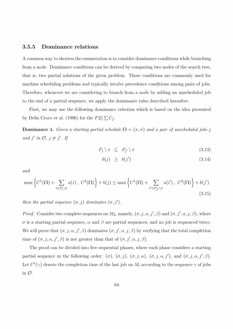
3.5.5 Dominance relations
A common way to shorten the enumeration is to consider dominance conditions while branching
from a node. Dominance conditions can be derived by comparing two nodes of the search tree,
that is, two partial solutions of the given problem. These conditions are commonly used for
machine scheduling problems and typically involve precedence conditions among pairs of jobs.
Therefore, whenever we are considering to branch from a node by adding an unscheduled job
to the end of a partial sequence, we apply the dominance rules described hereafter.
First, we may use the following dominance criterion which is based on the idea presented
by Della Croce et al. (1996) for the F2||∑Cj .
Dominance 1. Given a starting partial schedule Ω = (π,σ) and a pair of unscheduled jobs j
and j′ in O, j 6= j′. If
Pj \ π ⊆ Pj′ \ π (3.13)
b(j) ≥ b(j′) (3.14)
and
maxC1(Ω) +
∑i∈Pj\π
a(i) , C2(Ω)+ b(j) ≤ max
C1(Ω) +
∑i′∈Pj′\π
a(i′) , C2(Ω)+ b(j′)
(3.15)
then the partial sequence (σ, j) dominates (σ, j′).
Proof. Consider two complete sequences onM2, namely, (σ, j,α, j′, β) and (σ, j′,α, j, β), where
σ is a starting partial sequence, α and β are partial sequences, and no job is sequenced twice.
We will prove that (σ, j,α, j′, β) dominates (σ, j′,α, j, β) by verifying that the total completion
time of (σ, j,α, j′, β) is not greater than that of (σ, j′,α, j, β).
The proof can be divided into five sequential phases, where each phase considers a starting
partial sequence in the following order: (σ), (σ, j), (σ, j,α), (σ, j,α, j′), and (σ, j,α, j′, β).
Let Ci(γ) denote the completion time of the last job on Mi according to the sequence γ of jobs
in O.
64
Phase 1: The completion times of jobs in σ are identical for both sequences, i.e., for both
(σ, j,α, j′, β) and (σ, j′,α, j, β).
Phase 2: Due to (3.13) and (3.15), we have that C1(σ, j) ≤ C1(σ, j′) and C2(σ, j) ≤
C2(σ, j′).
Phase 3: Consider a starting partial sequence (σ, j, j′,α). Together with (3.13) we can
establish that
C1(σ, j,α) ≤ C1(σ, j, j′,α) = C1(σ, j′,α) (3.16)
Due to (3.15) and (3.16), we have that
C2(σ, j,α) ≤ C2(σ, j′,α) (3.17)
Phase 4: The completion time of the last job on M1 is identical in the two sequences
(σ, j,α, j′) and (σ, j′,α, j), i.e.,
C1(σ, j,α, j′) = C1(σ, j′,α, j) (3.18)
Due to (3.14), (3.17), and (3.18), we have that
maxC1(σ, j,α, j′),C2(σ, j,α)
+ b(j′) ≤ max
C1(σ, j′,α, j),C2(σ, j′,α)
+ b(j) (3.19)
That means that
C2(σ, j,α, j′) ≤ C2(σ, j′,α, j) (3.20)
Phase 5: When all predecessor jobs are completed of the starting partial sequences (σ, j,α, j′)
and (σ, j′,α, j), due to (3.18) we have that the completion time of each remaining job in I
is the same for both complete sequences, i.e., for both (σ, j,α, j′, β) and (σ, j′,α, j, β). Thus
together with (3.20) we have that
C2(σ, j,α, j′, β) ≤ C2(σ, j′,α, j, β) (3.21)
As a conclusion (σ, j,α, j′, β) will result in a total completion time that is not greater than
that of (σ, j′,α, j, β).
65

The following dominance criterion is based on the study by Della Croce et al. (2002) on the
F2||∑Cj problem. The key idea is that under certain conditions we can immediately identify
the next job to sequence.
Dominance 2. Given a starting sub-schedule Ω = (π,σ) of an optimal solution, if there exists
a job j ∈ σ such that
b(j) = minj′∈σ
b(j′)
(3.22)
∑i∈Pj\π
a(i) = minj′∈σ
∑
i′∈Pj′\πa(i′)
(3.23)
and
∑i∈Pj\π
a(i) ≤ b(j) (3.24)
then (σ, j) is a starting subsequence of an optimal solution.
A proof sketch is provided in the following. Suppose that in an optimal solution there is a
partial sequence α of r jobs in O \ σ, j immediately after σ and before j, that is, we consider
the sequence (σ,α, j). If we reinsert j before α and rearrange jobs onM1 according to Property
2, then all r jobs in α are moved to the right by at most b(j) time units. At the same time, the
completion time of job j is reduced by at least r · b(j) time units. Hence, the total completion
time of (σ, j,α) is not worse than that of (σ,α, j).
If more than one such job exists that satisfy the criteria in Dominance 2, then we may
arbitrarily choose the job with the lowest index.
Moreover, whenever a new job j ∈ O is appended at the end of a partial sequence resulting
in the current subsequence σ, we call an operator that changes the order of the scheduled jobs
and as a result we obtain a new sequence σ∗, which is compared with the current one. The
condition applied to our problem is based on the well-known dynamic programming dominance
66

property presented by Potts and Van Wassenhove (1983). When evaluating whether one se-
quence dominates the other we apply a generalization of the dynamic programming dominance
criterion presented by Della Croce et al. (2002).
We outline the key idea in the following. Suppose that σ∗, which is a permutation of the
jobs in σ, has a smaller total completion time and a greater makespan than that of σ. The
greater makespan of σ∗ implies that the total completion time of the remaining (unscheduled)
jobs that extend σ∗ is greater than or equal to that of σ. However, if the difference between
the two total completion times of the already scheduled jobs offsets the difference in the total
completion times related to the remaining jobs, then σ∗ dominates σ.
Dominance 3. (Della Croce et al., 2002) Given two partial schedules Ω = (π,σ) and Ω∗ =
(π∗,σ∗), such that σ∗ is a permutation of the jobs in σ, σ 6= σ∗. If
∑j∗∈σ∗
C(j∗) ≤∑j∈σ
C(j) (3.25)
and
|σ| ·[C2(Ω∗)−C2(Ω)
]≤∑j∈σ
C(j)−∑j∗∈σ∗
C(j∗) (3.26)
then σ∗ dominates σ.
A proof sketch is provided in the following. Assume that the jobs in σ are sequenced
arbitrarily. We show the total completion time of the complete sequence (σ∗, σ) is not greater
than that of the complete sequence (σ, σ). Let Ci(γ) denote the completion time of the last
job on Mi according to the sequence γ of jobs in O. We note that C1(σ∗,α) = C1(σ,α) for
any partial sequence α, such that α is a starting subsequence of σ. We can distinguish two
cases based on the value of ∆ := C2(Ω∗)−C2(Ω). First, the case that ∆ ≤ 0 is trivial. We
consider the case that ∆ > 0 from now on. For all j ∈ σ, we have that
C2(σ∗,α, j) = maxC1(σ∗,α, j) , C2(σ∗,α)
+ b(j) (3.27)
≤ maxC1(σ,α, j) , C2(σ,α) + ∆
+ b(j) ≤ C2(σ,α, j) + ∆ (3.28)
67
Now, consider the total of |σ| remaining jobs. Let ∑j∈σ Cσ(j) denote the total completion
time of jobs in the partial sequence σ, where the complete sequence is (σ, σ), i.e., jobs in σ are
sequenced after the starting sequence σ. Due to (3.28), we have that∑j∈σ
Cσ∗(j) ≤∑j∈σ
(Cσ(j) + ∆
)=∑j∈σ
Cσ(j) + |σ| ·[C2(Ω∗)−C2(Ω)
](3.29)
Together with (3.26) we have that∑j∈σ
Cσ∗(j)−∑j∈σ
Cσ(j) ≤∑j∈σ
C(j)−∑j∗∈σ∗
C(j∗) (3.30)
After rearranging, we obtain ∑j∗∈σ∗ C(j∗) +
∑j∈σ Cσ∗(j) ≤
∑j∈σ C(j) +
∑j∈σ Cσ(j) and
hence σ∗ dominates σ.
In case both conditions, namely, (3.25) and (3.26), happen to be equalities in Dominance
3, then we choose arbitrarily one of the sequences.
Dominance 3 is used as follows. Let j denote the last job in σ. Following Della Croce
et al. (2002), we apply the following operators to obtain a permutation of jobs in σ for all jobs
j′ ∈ σ \ j: (i) j is exchanged with j′, (ii) j is re-inserted immediately before j′, and (iii) j′ is
re-inserted after j. Then each pair consisting of the new starting sequence σ∗ and the original
σ is compared using Dominance 3.
3.6 Computational experiments
The branch-and-bound procedure was coded in C++. The instances were run on a P8700, 2.53
GHz computer with 4GB of RAM.
The number of jobs is chosen such that m ∈ 15, 20, 25, 30 and n ∈ 10, 15, 20, 25, 30. For
each instance, a transshipment matrix is generated randomly with a preset probability p that
a truck i ∈ I is a predecessor of some j ∈ O. We set p identical for all inbound and outbound
truck pairs within one instance, i.e., i ∈ Pj with probability p for all i ∈ I, o ∈ O. Should
the generated instance contain a truck with empty predecessor or successor set, the instance is
discarded and another is generated.
68

In the literature about the mean completion time flow shop problems, the processing times
for each job are typically taken from the uniform distribution U [1, 10] (cf. van de Velde, 1990;
Della Croce et al., 2002; Akkan and Karabatı, 2004) or U [1, 99] (cf. Taillard, 1993; Framinan
et al., 2003; Pan and Ruiz, 2013). The latter distribution is known to produce difficult problem
instances (Framinan et al., 2005). We follow the convention and generate the instances applying
these two distributions. For each problem size, 20 instances were randomly generated.
Table 3.3 presents results for instances with processing times in U [1, 10]. The CPU times
are given in seconds. Under ‘No. of nodes’, we report the number of nodes in the search tree.
As expected, the number of nodes and the CPU time are strongly correlated. Therefore, if
one aims to reduce the computation time, it is appropriate to consider also on the reduction
of the number of nodes, which is facilitated with the selected depth first search strategy in our
approach.
The results show that our procedure provides an optimal solution in a reasonable time for
instances with up to 25 outbound trucks if processing times are in the range U [1, 10].
Table 3.4 presents results for instances with processing times in U [1, 99]. The computational
time is greater compared to the case with processing times in U [1, 10].
We note that due to the capacity of the trucks carrying pallets or cases in a cross-dock envi-
ronment, the number of outbound trucks served per inbound truck is often bounded in practice.
Therefore, as the number of trucks increases (and exceeds a threshold level corresponding to
the capacity of the trucks), the value of p tends to 0. In the literature, there is only a limited
amount of information about the density of the transshipment matrix. In the study of Gue
(1999), the inbound trucks at a considered test site contain products for an average of 6.4 des-
tinations. In case of 25 inbound and 25 outbound trucks this yields that p = 0.26 on average,
assuming no correlation between the loads. The results show that instances of this moderate
size can be solved optimally by our algorithm within a reasonable time.
Among the problem parameters, the value of p seems to have the biggest impact on the
computation time. Figure 3.4 illustrates the change in CPU times and number of nodes when
69

Table 3.3: Average results for instances with processing times in U [1, 10]
p = 0.25 p = 0.5CPU No. of nodes CPU No. of nodes(sec) (×1000) (sec) (×1000)
m n avg max avg max avg max avg max15
10 0.0 0.0 0.2 1.1 0.0 0.0 0.0 0.115 0.2 2.0 3.6 23.7 0.0 0.0 0.2 0.420 0.2 1.0 3.6 11.1 0.0 0.0 0.2 0.825 0.7 7.0 8.0 55.1 0.0 0.0 0.3 0.730 1.6 7.0 13.8 50.7 0.0 0.0 0.6 1.5
2010 0.0 0.0 0.5 3.5 0.0 0.0 0.1 0.515 0.2 2.0 1.9 13.7 0.0 0.0 0.3 1.120 2.1 15.0 14.1 92.9 0.0 0.0 0.8 3.225 8.5 28.0 43.0 138.5 0.0 0.0 1.1 2.730 37.9 290.0 168.3 1226.8 0.1 1.0 1.5 5.3
2510 0.0 0.0 0.7 2.6 0.0 0.0 0.1 0.615 0.7 5.0 5.0 25.5 0.0 0.0 0.4 1.020 6.3 28.0 27.1 112.2 0.0 0.0 0.9 2.725 24.8 112.0 89.9 402.6 0.0 0.0 1.1 2.430 147.9 595.0 461.6 1963.8 0.3 2.0 2.5 7.9
3010 0.0 0.0 0.7 1.6 0.0 0.0 0.2 1.215 6.9 60.0 26.2 200.2 0.0 0.0 0.6 2.120 24.9 121.0 64.6 283.0 0.1 1.0 1.1 3.625 114.0 317.0 293.1 845.9 0.6 3.0 2.6 8.330 504.7 3154.0 1202.5 8406.0 0.9 4.0 3.0 10.1
0.0 CPU time indicates that the computation time is < 0.05 sec.
p is between 0.1 and 1. The computation time seems to increase exponentially as p decreases.
We note that as p decreases, the difference reduces between the optimal solution value for an
instance I for the [E2|tλ=0|∑Cj ] and the one for an instance I ′ for the F2||∑Cj , which is
generated based on I (see Section 3.4). This is due to the decrease in the number of predecessor
relations. On the other hand, when p = 1, an optimal solution is obtainable in polynomial
70

Table 3.4: Average results for instances with processing times U [1, 99]
p = 0.25 p = 0.5CPU No. of nodes CPU No. of nodes(sec) (×1000) (sec) (×1000)
m n avg max avg max avg max avg max15
10 0.0 0.0 0.5 3.2 0.0 0.0 0.1 0.215 0.4 4.0 5.5 37.8 0.0 0.0 0.2 0.520 0.3 1.0 4.8 12.7 0.0 0.0 0.4 1.125 0.7 8.0 9.6 69.5 0.0 0.0 0.5 1.330 1.9 7.0 16.2 52.2 0.0 0.0 0.8 2.4
2010 0.0 0.0 1.2 6.4 0.0 0.0 0.1 1.115 0.4 5.0 4.6 36.8 0.0 0.0 0.6 1.820 5.2 31.0 30.4 179.9 0.1 1.0 1.4 6.525 17.2 84.0 92.1 427.4 0.2 1.0 2.3 7.730 59.1 443.0 273.6 1966.4 0.4 3.0 2.9 17.3
2510 0.1 1.0 2.0 8.7 0.0 0.0 0.4 2.415 4.6 39.0 21.6 168.5 0.0 0.0 0.9 3.220 23.7 146.0 96.2 559.9 0.3 1.0 2.5 6.925 75.8 396.0 273.9 1379.9 0.3 1.0 2.4 6.730 330.1 946.0 1081.6 3313.8 1.2 4.0 5.2 17.7
3010 0.3 1.0 2.8 5.7 0.1 1.0 0.7 3.415 61.2 417.0 195.4 1342.3 0.2 1.0 1.5 5.020 133.6 996.0 349.8 2476.7 0.6 6.0 3.0 20.425 423.1 944.0 1163.5 2509.6 1.8 9.0 6.2 23.630 - - - - 2.3 11.0 6.4 31.3
0.0 CPU time indicates that the computation time is < 0.05 sec.- indicates that the values were not computed
time (see Section 3.3).
We have tested the performance of the proposed algorithm on randomly generated F2||∑Cj
problems. The results are presented in Table 3.5. For each configuration, 20 problem instances
were generated with processing times in U [1, 10]. The results show that an optimal solution is
71
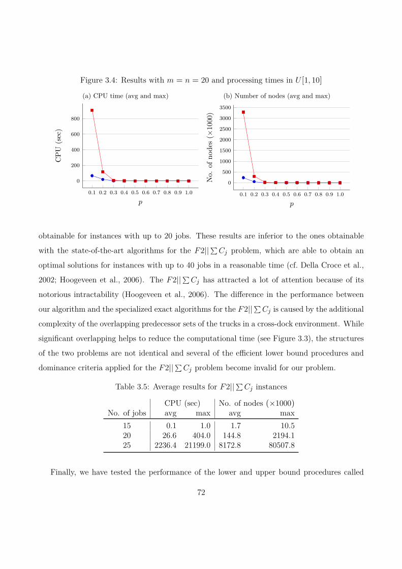
Figure 3.4: Results with m = n = 20 and processing times in U [1, 10]
(a) CPU time (avg and max)
0.1 0.2 0.3 0.4 0.5 0.6 0.7 0.8 0.9 1.0
0
200
400
600
800
p
CPU
(sec)
(b) Number of nodes (avg and max)
0.1 0.2 0.3 0.4 0.5 0.6 0.7 0.8 0.9 1.0
0
500
1000
1500
2000
2500
3000
3500
pNo.
ofno
des(×
1000
)
obtainable for instances with up to 20 jobs. These results are inferior to the ones obtainable
with the state-of-the-art algorithms for the F2||∑Cj problem, which are able to obtain an
optimal solutions for instances with up to 40 jobs in a reasonable time (cf. Della Croce et al.,
2002; Hoogeveen et al., 2006). The F2||∑Cj has attracted a lot of attention because of its
notorious intractability (Hoogeveen et al., 2006). The difference in the performance between
our algorithm and the specialized exact algorithms for the F2||∑Cj is caused by the additional
complexity of the overlapping predecessor sets of the trucks in a cross-dock environment. While
significant overlapping helps to reduce the computational time (see Figure 3.3), the structures
of the two problems are not identical and several of the efficient lower bound procedures and
dominance criteria applied for the F2||∑Cj problem become invalid for our problem.
Table 3.5: Average results for F2||∑Cj instances
CPU (sec) No. of nodes (×1000)No. of jobs avg max avg max
15 0.1 1.0 1.7 10.520 26.6 404.0 144.8 2194.125 2236.4 21199.0 8172.8 80507.8
Finally, we have tested the performance of the lower and upper bound procedures called
72
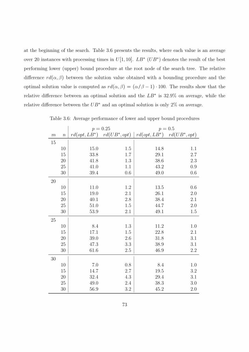
at the beginning of the search. Table 3.6 presents the results, where each value is an average
over 20 instances with processing times in U [1, 10]. LB∗ (UB∗) denotes the result of the best
performing lower (upper) bound procedure at the root node of the search tree. The relative
difference rd(α, β) between the solution value obtained with a bounding procedure and the
optimal solution value is computed as rd(α, β) = (α/β − 1) · 100. The results show that the
relative difference between an optimal solution and the LB∗ is 32.9% on average, while the
relative difference between the UB∗ and an optimal solution is only 2% on average.
Table 3.6: Average performance of lower and upper bound procedures
p = 0.25 p = 0.5m n rd(opt,LB∗) rd(UB∗, opt) rd(opt,LB∗) rd(UB∗, opt)15
10 15.0 1.5 14.8 1.115 33.8 1.7 29.1 2.720 41.8 1.3 38.6 2.325 41.0 1.1 43.2 0.930 39.4 0.6 49.0 0.6
2010 11.0 1.2 13.5 0.615 19.0 2.1 26.1 2.020 40.1 2.8 38.4 2.125 51.0 1.5 44.7 2.030 53.9 2.1 49.1 1.5
2510 8.4 1.3 11.2 1.015 17.1 1.5 22.8 2.120 39.0 2.6 31.8 3.125 47.3 3.3 38.9 3.130 61.6 2.5 46.9 2.2
3010 7.0 0.8 8.4 1.015 14.7 2.7 19.5 3.220 32.4 4.3 29.4 3.125 49.0 2.4 38.3 3.030 56.9 3.2 45.2 2.0
73
To summarize, for this complex problem in a cross-dock environment the results show that
our exact approach is able to solve instances of moderate size in a reasonable time.
3.7 Conclusions
This paper studies the problem of scheduling inbound and outbound vehicles with the objective
of minimizing the total completion time in a single inbound and single outbound dock cross-
docking environment with temporary storage. The performance measure improves the cross-
dock’s responsiveness and is known to lead to stable or balanced utilization of resources, rapid
turn-around of vehicles, and reduction of in-process inventory (Rajendran and Ziegler, 1997;
Framinan and Leisten, 2003).
Our solution approach is based on the relation of the problem with machine scheduling.
Indeed, the problem is a generalization of a well-studied NP -hard problem, the two-machine
flow shop problem, i.e., F2||∑Cj . We present optimality properties, three lower bound pro-
cedures, and propose an exact branch-and-bound algorithm, in which we branch on the new
outbound trucks that are appended to a partial outbound truck sequence.
To the best of our knowledge, this is the first exact approach to the problem. The compu-
tational experiments show that when the transshipment matrix is dense, the proposed branch-
and-bound algorithm can provide proven optimal solutions within seconds for problems with up
to 60 outbound trucks. However, if the number of trucks increases and/or the transshipment
matrix becomes sparse, the computation time increases rapidly. The results show that the
procedure is able to find optimal solutions for moderate size instances of 40-50 trucks within a
reasonable time.
While cross-dock facilities with a single inbound and a single outbound dock are rare in
practice, the solution approach can be used as a building block for solving more complex
problems. In particular, for problems where the truck-to-dock assignment is done prior to
truck sequencing. Furthermore, it seems that the upper bound algorithms implemented at the
74

beginning of the search obtain good solutions. It is thus of interest to study other complex
truck-scheduling problems in a cross-dock environment and search for heuristic approaches that
are able to provide near-optimal solutions.
75


Chapter 4
Scheduling Trucks in a Cross-Dock with Mixed
Service Mode Dock Doors

Scheduling Trucks in a Cross-Dock with Mixed Service Mode DockDoors
Peter Bodnar† and René de Koster∗
† CORAL, Department of Economics and Business, Aarhus University, Denmark
[email protected]∗ Rotterdam School of Management, Erasmus University, Netherlands
Abstract
The problem considered in this paper is to schedule inbound and outbound trucks
subject to time windows at a multi-door cross-dock in which an intermixed sequence of
inbound and outbound trucks can be processed at the dock doors. We focus on operational
costs by considering the cost of handling temporarily stored products, as well as the
cost of tardiness due to processing outbound trucks after their respective due dates. A
mathematical model for optimal solution is derived and an adaptive large neighborhood
search heuristic is proposed to compute near-optimal solutions of real size instances.
Computational experiments show that the proposed heuristic algorithm can obtain high
quality solutions within short computation times.
78

4.1 Introduction
Cross-docking is a process that aims to minimize the inventory-holding function of a warehouse
by rapidly consolidating shipments from diverse sources with known destinations and transfer-
ring them to outbound trucks such that in-between storing is minimized. Nevertheless, between
unloading and loading, products might be stored temporarily (e.g., for a few hours) to wait for
a truck to arrive (Vis and Roodbergen, 2008). In a recent survey with 219 respondents, only
20.6% of those currently cross-docking practice pure cross-docking, i.e., cross-docking without
temporary storage; most respondents first temporarily store products in the warehouse (Sad-
dle Creek Corporation, 2011). Shipments typically spend less than 24 hours at the facility,
sometimes less than an hour (Bartholdi III and Gue, 2004).
One may divide cross-docking operations by the handling units (Bartholdi III et al., 2008):
in case-pick cross-docking, the distributor receives pallets of product and ships cases, or even
individual items; while unit-load cross-docking is exclusively about processing unit size prod-
ucts. In this paper, we investigate cross-dock systems that are devoted entirely to unit-load
handling.
According to Bartholdi III and Gue (2004) the first design decision is the total number of
docks. Two types of docks are considered: inbound docks (also called receiving doors), where
trucks dock to be unloaded, and outbound docks (also called shipping doors), where trucks
dock to collect freight for a specific destination. Studies on cross-docking tend to make the
assumption that facilities designed for cross-docking are long, narrow rectangles (I-shape), in
which the docks are positioned on two opposite sides of the facility such that one side of the
cross-dock is the ‘inbound side’ where inbound trucks are processed, and another side is the
‘outbound side’ where outbound trucks are processed, that is, products are moved across the
facility (cf. Bartholdi III and Gue, 2000; Van Belle et al., 2012; Bellanger et al., 2013).
In the aforementioned survey, however, only 53.7% of the respondents who cross-dock today
use facilities that are specifically designed or set up for cross-docking and just 27.3% of those
planning to cross-dock in the near future expect to use such a facility (Saddle Creek Corpo-
79
ration, 2011). This implies that the typical material flow may not necessary be characterized
with an ‘I’ shape, in which products are moved from dedicated inbound to dedicated outbound
docks. Moreover, not distinguishing between dock types is reasonable, since docks are primarily
designed for generic trucks, i.e., docks are ’flexible’ by design and can be operated in a mixed
service mode (cf. Shakeri et al., 2012). A typical dock can be used either as an inbound or as
an outbound dock at any time.
However, utilizing dock flexibility may impose complexity from a managerial point of view.
Bartholdi III and Gue (2000) report that most terminals conduct inbound and outbound op-
erations, so named because of the type of freight handled. Unloading and loading procedures
may involve different equipment and handling requirements may differ substantially. Moreover,
requested employee competencies may also differ in the two procedures, a fact that must be
taken into consideration especially if the organization opts for flexible or temporary employees.
Therefore, when mixed service mode docks are used, the complexity of managerial decisions is
likely to increase. On the other hand, flexibility should be designed into every function and
operation of the warehouse (Brockmann and Godin, 1997). Hence, it is of interest to investigate
the potential of utilizing the inherent flexibility to increase the efficiency and reduce costs.
In this paper, we focus on truck scheduling with the objective to minimize the operational
costs, consisting of storage, retrieval and tardiness costs. The cost of storage and retrieval
relates to those loads that are placed in the temporary storage area instead of being directly
loaded on outbound trucks. The cost of tardiness is considered due to an obvious priority of
any cross-dock, that is, to respect the truck due times agreed with the customers.
The contribution of this research is twofold. First, we derive a mathematical model that
can be used to obtain optimal solution for instances of moderate size. We show that the
problem isNP-hard. Therefore, for large instances, we propose an adaptive large neighborhood
search based approach, which is shown to provide good quality solutions. Second, we take into
consideration the potential of mixed service mode docks in a cross-docking environment. In
particular, we investigate the effect of utilizing a subset of docks in a mixed service mode and
80
evaluate their impact with respect to the operational costs.
In the next section, we present the related literature. In Section 4.3, we describe the
problem. Our model is presented in Section 4.4. Then, in Section 4.5, the proposed heuristic
procedure is described. Results of the computational experiments are reported in Section 4.6.
Finally, conclusions are presented in Section 4.7.
4.2 Literature review
Several papers study cross-docking. For recent comprehensive literature reviews we refer to
Agustina et al. (2010), Boysen and Fliedner (2010) and Van Belle et al. (2012). Cross-dock
decisions include truck scheduling, assigning trucks to docks and products to locations. In this
section, we present literature related to these three areas.
The product-to-location assignment problem emerges in a cross-dock environment since
each arriving item has to be assigned to a storage location unless it is immediately transferred
to another truck. Several models assume that the products can be kept at the doors with
an infinite buffer capacity (Yu and Egbelu, 2008; Vahdani and Zandieh, 2010; Bellanger et al.,
2013). This may be a reasonable assumption when the ratio of trucks per door is low. However,
in case of a high ratio, products are stored in a separate temporary storage area to facilitate
the operations at the doors. This additional handling increases the operational costs. The
handling cost has been addressed by Vis and Roodbergen (2008) and Sadykov (2012). Vis and
Roodbergen (2008) consider the problem of determining the short-term storage locations such
that the total travel distance in the entire facility is minimized with the assumption of prior
truck scheduling and truck-to-dock assignment. Sadykov (2012) analyzes a single inbound and
single outbound door cross-dock with a temporary storage location and shows that the problem
of truck scheduling with the objective to minimize the storage usage is NP-hard in the strong
sense even for the case in which each inbound truck carries at most two product types, each
outbound truck carries at most one product type, all storage costs are unitary, and the storage
81

capacity is unlimited.
Truck-to-dock assignment is the problem of assigning inbound and outbound trucks to
docks. Note that the truck-to-dock assignment problem is different from the truck scheduling
problem, which takes the time dimension into account, while time is not considered in the
dock door assignment problem (Konur and Golias, 2013). The paper of Tsui and Chang (1990)
is among the first studies on the truck-to-dock assignment problem. The authors present a
bilinear objective formulation and provide a local search algorithm. For the same formulation,
Tsui and Chang (1992) describe a branch-and-bound solution approach. The paper of Oh et al.
(2006) presents the problem in the context of a mail distribution center and proposes a genetic
algorithm heuristic. Miao et al. (2009) consider the problem with operational time constraints
assuming that trucks are pre-scheduled with hard time windows during which a dock is fully
occupied. The investigated problem is NP-hard, hence tabu search and a genetic algorithm
are proposed in the paper.
Recently, several studies have addressed the problem from a scheduling point-of-view. The
objective function tends to be time-related, such as the minimization of makespan (Boysen
and Fliedner, 2010). Many studies focus on cross-docks with a single inbound and a single
outbound dock (Yu and Egbelu, 2008; Chen and Lee, 2009; Boysen et al., 2010; Soltani and
Sadjadi, 2010; Larbi et al., 2011).
For this configuration, Yu and Egbelu (2008) provide a mixed integer linear programming
formulation, assuming unlimited storage capacity in the cross-dock and propose a heuristic
method to minimize the makespan. For the same formulation, Vahdani and Zandieh (2010),
Boloori Arabani et al. (2011), and Liao et al. (2012) propose metaheuristic approaches. This
configuration has been extended by Boloori Arabani et al. (2010) and Boloori Arabani et al.
(2012); these studies include time windows and aim to minimize the earliness and tardiness,
for which metaheuristic methods are proposed.
Chen and Lee (2009) formulate the minimum makespan truck scheduling problem as a two-
machine flow-shop problem, where an operation on the first machine is to unload the inbound
82
products, while collecting those products and loading them into an outbound truck is considered
as an operation on the second machine. The authors assume that processing a truck on the
second machine cannot be started unless all the corresponding loads have been unloaded from
the trucks that are processed on the first machine. With reduction from the classical two-
machine flow-shop problem, Chen and Lee (2009) show that the problem is strongly NP-hard.
Moreover, the problem remains strongly NP-hard even if all processing times are unitary.
For the case when temporary storage is forbidden, Soltani and Sadjadi (2010) propose
two hybrid metaheuristics, i.e., hybrid simulated annealing and hybrid variable neighborhood
search, to solve the truck scheduling problem such that the makespan is minimized.
Boysen et al. (2010) present a novel formulation for the truck scheduling problem in a
single inbound, single outbound door cross-dock by assuming that the planning horizon is split
into time intervals. They show that the problem is NP-hard even for a restricted case, in
which all handling operations per truck are completed within a single time interval, internal
transportation time is ignored, and the intermediate buffer is not limited in size.
The above mentioned studies provide insights and may be used as building blocks in an
approach to tackle a more general problem. However, cross-docks with a single inbound and
single outbound door are rare, thus studies on multi-door systems are necessary (Liao et al.,
2013).
The study of Chen and Song (2009) extends the work of Chen and Lee (2009) by considering
multiple machines corresponding to doors, and develops a heuristic solution approach. With
the objective to minimize makespan, Shakeri et al. (2012) consider a limited number of forklifts
inside the multi-door warehouse and address the truck scheduling problem with a heuristic
algorithm. A hybrid flow-shop model with the same objective function has been developed
for this problem context by Bellanger et al. (2013). The authors present a branch-and-bound
method for small and a heuristic for real size instances.
For the case when time windows are considered, finding schedules to minimize earliness and
tardiness has been addressed by Li et al. (2004). The authors provide a two-phase parallel
83

machine formulation and develop two genetic algorithm based methods, one of which uses
integer programming to solve an embedded subproblem. An alternative approach is presented
for the same problem by Álvarez Pérez et al. (2009) based on tabu search.
Boysen (2010) analyzes the case when no storage is available in the multi-door cross-dock.
The proposed bounded dynamic programming and simulated annealing algorithms aim to min-
imize three objectives, namely flow time, processing time, and tardiness, assuming that the ser-
vice times over all trucks do not deviate significantly. The time is discretized into fixed-length
periods, which are sufficiently long to process an inbound truck. Due to the zero-inventory
policy the outbound truck schedule can be easily derived given an inbound truck schedule.
Alpan et al. (2011) and Alpan et al. (2011) analyzed the truck scheduling problem with a
focus on operational costs. In particular, the focus is on minimizing the sum of handling cost
and outbound truck preemption cost. The authors present a bounded dynamic programming
and a heuristic approach, while assuming discretized time.
In this study, we address the truck scheduling problem and extend the paper of Boysen
et al. (2010) with the main difference being that we take a direct focus on operational costs
and consider a multi-door cross-dock environment. We show that the problem is NP-hard and
present a heuristic approach that follows the adaptive large neighborhood search (ALNS) prin-
ciples (Ropke and Pisinger, 2006a). ALNS has been successfully applied in complex scheduling
problems, including vehicle routing problems (Ropke and Pisinger, 2006b; Pisinger and Ropke,
2007; Stenger et al., 2013) and crane scheduling in container terminals (Gharehgozli et al.,
2013).
Our study differs from most of the previous studies on truck scheduling in a multi-door
cross-dock in the following aspects: (i) the objective is to minimize operation costs, namely,
the sum of handling and tardiness costs, and (ii) a set of doors can function in a mixed service
mode.
84
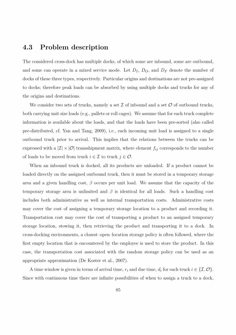
4.3 Problem description
The considered cross-dock has multiple docks, of which some are inbound, some are outbound,
and some can operate in a mixed service mode. Let DI , DO, and DF denote the number of
docks of these three types, respectively. Particular origins and destinations are not pre-assigned
to docks; therefore peak loads can be absorbed by using multiple docks and trucks for any of
the origins and destinations.
We consider two sets of trucks, namely a set I of inbound and a set O of outbound trucks,
both carrying unit size loads (e.g., pallets or roll cages). We assume that for each truck complete
information is available about the loads, and that the loads have been pre-sorted (also called
pre-distributed, cf. Yan and Tang, 2009), i.e., each incoming unit load is assigned to a single
outbound truck prior to arrival. This implies that the relations between the trucks can be
expressed with a |I| × |O| transshipment matrix, where element fij corresponds to the number
of loads to be moved from truck i ∈ I to truck j ∈ O.
When an inbound truck is docked, all its products are unloaded. If a product cannot be
loaded directly on the assigned outbound truck, then it must be stored in a temporary storage
area and a given handling cost, β occurs per unit load. We assume that the capacity of the
temporary storage area is unlimited and β is identical for all loads. Such a handling cost
includes both administrative as well as internal transportation costs. Administrative costs
may cover the cost of assigning a temporary storage location to a product and recording it.
Transportation cost may cover the cost of transporting a product to an assigned temporary
storage location, stowing it, then retrieving the product and transporting it to a dock. In
cross-docking environments, a closest–open–location storage policy is often followed, where the
first empty location that is encountered by the employee is used to store the product. In this
case, the transportation cost associated with the random storage policy can be used as an
appropriate approximation (De Koster et al., 2007).
A time window is given in terms of arrival time, ri and due time, di for each truck i ∈ I,O.
Since with continuous time there are infinite possibilities of when to assign a truck to a dock,
85
the time will be divided into time intervals. Let T denote the set of time intervals. The
determination of the time interval length is driven by the expected length of loading and
unloading operations (cf. Boysen et al., 2010; Boysen, 2010). We assume that for each truck
the processing takes the same amount of time, and all scheduled transshipment operations are
completed in one time interval with sufficient workforce. This can be seen as a reasonable
approximation of reality, whenever the number of loads per vehicle does not vary strongly
(Boysen, 2010).
Preemption of a docked truck is not allowed. That is, once the processing of a truck begins
the truck is kept at the dock until its completion. Trucks can be processed in a single time
interval, hence when an inbound truck is docked it is completed within the same time interval.
However, the completion time of an outbound truck depends on the load arrivals. In particular,
the processing of an outbound truck can be completed only after each load for that truck has
been unloaded from a set of inbound trucks. Whenever the loading of an outbound truck is
completed after its due time, the total cost increases due to the tardiness. We assume that the
cost γ of tardiness per time interval is known. Such cost depends on the agreed due time of an
outbound truck, which may be determined internally, driven by the working hours and internal
schedule of the cross-dock, or externally, e.g., by the customer. Moreover, the cost per time
unit may include other factors, e.g., overtime hours, an agreement with specified indemnity, or
an estimated loss in value for the customer. Tardy completion of an outbound truck may lead
to tardy delivery to the customer, i.e., poor service performance, which may result in loss of
goodwill for the cross-dock. In this study, we assume that γ is the same for all trucks. However,
including different values is easily achievable in the proposed model.
Our purpose is to find a schedule both for the inbound and outbound trucks so that the
sum of handling and tardiness costs is minimized. The objective function is a trade-off between
the two considered costs. We have the following decisions to make at each time interval: (i)
select some outbound trucks to be processed, (ii) select some inbound trucks to be processed.
Figure 4.1 presents a cross-dock example with six docks, three of which are currently used
86
by inbound trucks and three are used by outbound trucks. The temporary storage area is
presented as a shaded rectangle. The transportation flow is indicated with dotted lines.
truck # 1 truck # 2 truck # 3 truck # 4 truck # 5 truck # 6
SKU
#1
SKU
#2
SKU
#4
SKU
#6
SKU
#6
SKU
#1
SKU
#1
SKU
#1
SKU
#2
SKU
#3
SKU
#5
SKU
#3
SKU
#4
SKU
#4
SKU
#6
SKU
#6SKU
#4
SKU
#5
Figure 4.1: A representation of material flow in a cross-dock with temporary storage area
When docks are mainly used for outbound flows, then the cost of handling is reduced since
unit loads are likely to be transported directly to the outbound trucks. However, in this case
only a few docks are available for inbound trucks and this may result in a bottleneck for the
inbound flow. As a consequence, outbound trucks may be completed late and thus the total
cost of tardiness may increase.
When docks are mainly used for inbound flows, then the unit loads may have to be stored
temporarily, and thus handled twice. That is, the total cost of handling increases. Nevertheless,
products ‘flow’ into the cross-dock rapidly, which may provide increased flexibility for the
scheduling of the outbound trucks which can result in lower total tardiness cost.
4.4 Model formulation
A mathematical programming model can be formulated to the problem, which is referred to as
the full problem (FP). The following notations are used:
I set of inbound trucks
87
O set of outbound trucks
T set of time intervals
DI number of dedicated inbound docks
DO number of dedicated outbound docks
DF number of flexible docks
fij number of unit loads on i ∈ I associated with j ∈ O
ri arrival time of truck i ∈ I,O
di due time of truck i ∈ I,O
β handling cost per unit load
γ tardiness cost per time interval for outbound trucks
Additionally, the following notations are used to simplify the formulation:
δtj is computed as δtj = max0, t− dj, ∀j ∈ O, t ∈ T ,
T Ei set of time intervals before truck i arrives, i.e., T Ei = t|t ∈ T , t < ri, ∀i ∈ I,O
T Li set of time intervals after the due time of truck i, i.e., T Li = t|t ∈ T , di < t, ∀i ∈ I,O
Variables:
xti is 1 if inbound truck i ∈ I is processed at time interval t ∈ T and 0 otherwise
ytj is 1 if outbound truck j ∈ O is processed at time interval t ∈ T and 0 otherwise
ytj is 1 if the loading of outbound truck j ∈ O is completed at t ∈ T and 0 otherwise
stj total number of units in the storage area for j ∈ O at (the end of) t ∈ T
ltj total number of units loaded on j ∈ O at (the end of) t ∈ T
sti increment in the number of units stored in the storage area for i ∈ O at t ∈ T ,
when compared to the previous time interval
The objective of the presented problem is to minimize the total cost, which is defined as
88

the sum of handling and tardiness costs. The formulation of the FP is the following:
min∑t∈T
∑j∈O
(βstj + γδtj y
tj
)(4.1)
subject to
∑i∈I
xti +∑j∈O
ytj ≤ DI +DF +DO ∀t ∈ T (4.2)
∑i∈I
xti ≤ DI +DF ∀t ∈ T (4.3)
∑j∈O
ytj ≤ DF +DO ∀t ∈ T (4.4)
di∑t=ri
xti = 1 ∀i ∈ I (4.5)
∑t∈T
ytj = 1 ∀j ∈ O (4.6)
st−1j + lt−1
j +∑i∈I
xt−1i fij = stj + ltj ∀j ∈ O, t ∈ T (4.7)
ltj − lt−1j ≤
∑i∈I
fijytj ∀j ∈ O, t ∈ T (4.8)
lt−1j ≤ ltj ∀j ∈ O, t ∈ T (4.9)
ytj ≤ ytj + yt+1j ∀j ∈ O, t ∈ T (4.10)∑
i∈Ifij y
tj ≤ ltj ∀j ∈ O, t ∈ T (4.11)
stj − st−1j ≤ stj ∀j ∈ O, t ∈ T (4.12)
xti = 0 ∀i ∈ I, t ∈ T Ei , T Li (4.13)
ytj = 0 ∀j ∈ O, t ∈ T Ei (4.14)
xti ∈ 0, 1 ∀i ∈ I, t ∈ T (4.15)
ytj , ytj ∈ 0, 1 ∀j ∈ O, t ∈ T (4.16)
stj , stj , ltj ∈ Z+ ∀j ∈ O, t ∈ T (4.17)
89
Constraints (4.2) ensure that the maximum number of docked trucks at any time interval is at
most the number of docks. Constraints (4.3) ensure that the number of inbound trucks docked
at any time interval is at most the number of docks that can be used to process inbound trucks.
Similarly, constraints (4.4) ensure that the maximum number of outbound trucks docked at
a given time interval t is at most the number of docks that can be used to process outbound
trucks. Constraints (4.5) ensure that each inbound truck is unloaded exactly once. This also
implies that inbound trucks cannot be used as temporary storage locations. Constraints (4.6)
ensure that all outbound trucks must be completed eventually. Constraints (4.7) ensure that
items that are unloaded from an inbound truck are either stored at the temporary storage area
or loaded on the associated outbound truck. We note that if β > 0 then at most one of stj and ltjis non-zero due to the objective function. Constraints (4.8) ensure that whenever an outbound
truck is loaded it must be docked. Constraints (4.9) ensure that the number of unit loads on
any outbound truck is non-decreasing. Constraints (4.10) ensure that the outbound trucks are
kept at the outbound docks until they are completed. Constraints (4.11) ensure that if an
outbound truck is completed, then all the unit loads for that truck are loaded. Constraints
(4.12) ensure that the increment of units for outbound truck j in the temporary storage is
computed as the (non-negative) difference of quantities stored in the temporary storage area.
Constraints (4.13) and (4.14) ensure that no truck can be docked before its arrival time, and
no inbound truck can be docked after its due time. Finally, constraints (4.15)–(4.17) specify
domains of decision and auxiliary variables.
The formulation can be tightened by ensuring that once an outbound truck is completed it
is not docked again:
t−1∑t′=1
yt′j + ytj ≤ 1 ∀j ∈ O, t ∈ T (4.18)
We note that one can easily extend the model to express different tardiness costs per trucks,
for example, by replacing the expression γδtj in (4.1) with arbitrary γtj , where γtj is the tardiness
cost of truck j ∈ O when it is completed at time t.
90

Boysen and Fliedner (2010) have introduced a 3-field notation [a|b|c] for cross-docking
scheduling problems, where a is door environment, b is the operational characteristics, and c is
the objective. The notation uses square brackets in order to clearly distinguish the considered
cross-docking problem from problems in a classical scheduling environment. Accordingly, our
problem can also be denoted as [EM|ri, pi = 1, di, tp = 0|∑Ti +∑Sp] , where EM indicates
that a subset of docks is operated in an exclusive (or dedicated) service mode and another
subset in a mixed service mode, ri is the arrival time, pi is the processing time of, and di is
the due time of truck i ∈ I,O. Furthermore, tp denotes the transshipment time inside the
cross-dock, ∑Ti is the total tardiness, and ∑Sp is the total number of loads placed in the
temporary storage.
Proposition 2. [EM|ri, pi = 1, di, tp = 0|∑Ti +∑Sp] is strongly NP-hard.
Proof. We transform instances of F2|CD, pik = 1|Cmax, which is known to be strongly NP-
hard (Chen and Lee, 2009), to [EM|ri, pi = 1, di, tp = 0|∑Ti+∑Sp] . We restate F2|CD, pik =
1|Cmax in the following.
F2|CD, pik = 1|Cmax Problem: There are two machines, M1 and M2, and two sets
of jobs, J1 = J11, J21, . . . , Jn1 and J2 = J12, J22, . . . , Jm2, where each Ji1, i =
1, . . . ,n must be processed onM1, and requires a processing time of pi1 = 1, and each
Jj2, j = 1, . . . ,m, must be processed onM2 and requires a processing time of pj2 = 1.
That is, pi1 = pj2 = 1 for all i and j. For each Jj2 in J2, there is a corresponding
subset of J1, call it Sj , such that Jj2 can be processed on M2 only after all jobs in
Sj have been completed on M1. We search for a sequence of jobs in J1 on M1 and
of jobs in J2 on M2 such that the makespan, i.e., the time between the start time
of processing the first job on M1 and the completion time of the last job on M2, is
minimized.Given an instance of F2|CD, pik = 1|Cmax and a positive integer M , the question
we ask is "can we find a feasible schedule F2|CD, pik = 1|Cmax with a makespan no
larger than M?"
91

Now, we construct an instance of [EM|ri, pi = 1, di, tp = 0|∑Ti +∑Sp] as follows. First, we
assume a single inbound and single outbound door cross-dock facility, i.e., DI = DO = 1 and
DF = 0. Moreover, β = 0 and ri = 0 ∀i ∈ I,O.
Corresponding to each job Ji1 in F2|CD, pik = 1|Cmax we construct a job i in I, thus
|I| = n. Corresponding to each job Jj2 in F2|CD, pik = 1|Cmax we construct a job j in O,
thus |I| = m. For each pair of jobs i = 1, . . . ,n and j = 1, . . . ,m, we have that fij = 1 if
Ji1 ∈ Sj and 0 otherwise.
Furthermore, let γ = 1, |T | ≥ maxM , |J1|+ |J2|, di = |T | ∀i ∈ I and dj = M ∀j ∈ O.
That is, the time window of any inbound truck i ∈ I spans the whole planning horizon, and
each outbound truck has the same due date at time M .
The question we ask is "can we find a feasible schedule to our problem [EM|ri, pi = 1, di, tp =
0|∑Ti +∑Sp] with a total cost not greater than 0?"
As the length of such an [EM|ri, pi = 1, di, tp = 0|∑Ti +∑Sp] instance is polynomially
bounded in |J1| · |J2|, it can be readily generated on the basis of any instance of F2|CD, pik =
1|Cmax in polynomial time.
→ A solution of any YES-instance of F2|CD, pik = 1|Cmax, i.e., for which a feasible
schedule exists with makespan no greater than M , is also feasible for [EM|ri, pi = 1, di, tp =
0|∑Ti+∑Sp] with total cost not greater than 0, since each truck is completed at time M at
the latest.
← Assume that there exists a feasible YES-instance of [EM|ri, pi = 1, di, tp = 0|∑Ti +∑Sp] (generated as described before), i.e., the total cost is not greater than 0. In such a
schedule, some outbound trucks can be docked for more than one time interval; let O denote
the set of such trucks, O ⊆ O. Since β = 0, the total cost depends only on the completion
time of the trucks; therefore, we can delay the start time of docking any j ∈ O until the time
interval when j is completed without changing the total cost. Using this delay operation on all
the trucks in O we obtain a schedule, in which each truck is processed only in one time interval.
The new schedule is still feasible for [EM|ri, pi = 1, di, tp = 0|∑Ti +∑Sp] without changing
92
the total cost. Recall that dj = M , ∀j ∈ O. The obtained schedule leads to a corresponding
F2|CD, pik = 1|Cmax, with a makespan no greater than M .
We can conclude that a solution with a total cost not greater than 0 exists if and only
if the corresponding instance of [EM|ri, pi = 1, di, tp = 0|∑Ti +∑Sp] is a YES-instance.
NP-hardness of our problem immediately follows.
The NP-hardness of our problem implies that the time requirement of an exact approach to
obtain an optimal solution increases exponentially as the size of the problem increases (unless
P = NP), hence exact algorithms are likely to be inefficient when the number of trucks is large.
Since we are interested in real-size instances, it is appropriate to develop algorithms which give
near-optimal solutions. Therefore, we propose a heuristic approach, which is explained in the
following section.
4.5 Metaheuristic approach
In order to find a good feasible solution for real-size instances, a heuristic has been devel-
oped that follows the principles of Adaptive Large Neighborhood Search (Ropke and Pisinger,
2006a,b; Pisinger and Ropke, 2007). As in Ropke and Pisinger (2006b), the master level search
framework is based on simulated annealing (SA). In the following, we first outline the frame-
work of the proposed approach. Second, we present a heuristic method to construct initial
feasible solutions. Then we define a schedule representation, which is used in the iterations
of an improvement heuristic. Finally, we describe the neighborhood operators, which are used
to modify the schedule in order to obtain improvements, along with a reduced problem for-
mulation to obtain a complete candidate solution, the acceptance of which is based on the SA
principles. The pseudo code of the heuristic is presented below in Algorithm 2.
The heuristic operates as follows. First, a set of feasible solutions, X is created. A solution
consists of an inbound truck schedule π and an outbound truck schedule σ. Let z(x) denote
the objective value of solution x. From X, we select a solution with the lowest objective value
93

and record it as the best found solution, x∗. Then, the heuristic iterates until the terminating
criterion is met.
In each iteration, the algorithm tries to find a solution with a lower objective value by first
changing a part of the solution, namely, π for which a set N of neighborhood operators has been
developed. In each iteration, a neighborhood operator n(·) ∈ N is selected in a probabilistic
manner, such that the better performance a neighborhood operator had previously, the more
likely it is to be selected in the successive iterations. This is achieved by using a roulette wheel
selection principle, where each n ∈ N has a probability corresponding to its weight µn. In
particular, n ∈ N is selected with probability µn/∑|N |i=1 µi. Then, an inbound truck schedule
π′ is selected from the neighborhood n(π).
Once π′ is given, the problem to obtain a new feasible solution x′ reduces to decide when
each outbound truck should be first docked since preemption is not allowed. We call the
resulting model a restricted problem, RP. The main difference between RP and FP, is that in
RP we search for an σ that minimizes the total cost given a π.
The current solution is updated following the SA principles, which have two key parameters,
namely, a temperature T and a cooling ratio r. A new feasible solution x′ is always accepted
if its objective value is better than that of x. Otherwise, x′ replaces x with a probability
of e−(z(x′)−z(x∗))/T . Following Ropke and Pisinger (2006a), the temperature is initialized as
T := −w · z(x∗)/ ln 0.5 where w is an arbitrary parameter and x∗ is the best found solution,
i.e., a solution that is w% worse than z(x∗) is accepted with probability 0.5 (cf. Kovacs et al.,
2012). Then T is updated using the recursion T := rT with 0 < r < 1. Furthermore, if within
the last nT consecutive iterations the current solution has not been improved, then we apply a
diversification strategy to direct the search into other regions of the solution space (cf. Stenger
et al., 2013). In particular, we reset the temperature T such that its new value is computed
the same way as the initial temperature. Finally, we set the terminating criterion such that a
total of 5,000 iterations are executed.
94
Algorithm 2 Pseudo code of the implemented heuristic
1 Construct a set of feasible initial solutions X2 Choose a x∗ ∈ X such that z(x∗) ≤ z(x0) ∀x0 ∈ X3 Set the current solution x← x∗
4 Construct an inbound truck schedule π corresponding to x
5 until stop criterion is met do6 Choose a neighborhood operator, n() ∈ N based on adaptive weights7 Choose an inbound truck schedule, π′ ∈ n(π)8 Apply RP to π′, resulting in x′9 if z(x′) < z(x∗) then10 Set x∗ ← x′
11 end if12 if z(x′) ≤ z(x) then13 Set π ← π′, x← x′
14 else if Uniform[0; 1) ≤ e−(z(x′)−z(x∗))/T then
15 Set π ← π′, x← x′
16 end if17 Update T18 Update the score of n()19 repeat
20 return x∗
4.5.1 Constructing an initial feasible solution
In this section we propose a heuristic algorithm that follows the principles presented in Yu and
Egbelu (2008) and can be used to create feasible solutions. The same set of assumptions holds
in this algorithm as in the FP.
The procedure iterates through the time intervals in T . In each time interval t ∈ T
a set of processed inbound trucks It and a set of docked outbound trucks Ot is created,
It ⊆ I and Ot ⊆ O. At the beginning of each iteration, we first initialize Ot := j | j ∈
Ot−1, j is not completed. Second, we define It, and finally, update Ot.
Defining It is done in two steps. In the first step, a set of candidate inbound trucks, C(I)t
95

is created. In particular,
C(I)t := i | i ∈ I, ri ≤ t ≤ di, i 6∈ ∪t′=t−1t′=0 It
′ (4.19)
In the second step, we define It ⊆ C(I)t based on decision rules that arise from the following
selection strategies: (i) select the truck with the earliest arrival time (FCFS), (ii) select the
truck with the earliest due time (EDD), (iii) select the truck with the largest number of units
transferred directly to outbound trucks (cf. Yu and Egbelu, 2008), and (iv) select the truck
that, when processed, completes the largest number of outbound trucks.
In the third strategy, we assign a weight, wi for each i ∈ C(I)t to denote the number of
units transferred directly to outbound trucks, and set wi :=∑j∈Ot fij + ∆i, where the first
part takes in consideration the already docked outbound trucks, while ∆i is based on the set
C(O)t of available but not yet docked outbound trucks, such that
C(O)t := j | j ∈ O, rj ≤ t, j 6∈ ∪t′=t−1t′=1 Ot
′ (4.20)
Let Sti denote the set of the first DO +DF − |Ot| outbound trucks when the elements in C(O)t
are sorted in non-increasing order of load units received from i. We then define ∆i :=∑j∈Sti
fij .
In the fourth strategy, the computation is similar to the previous one, expect that in this
case, we are interested in the number of outbound trucks that can be completed when an
inbound truck is processed.
Based on these four strategies we apply four decision rules to define It by selecting sequen-
tially, at most DI +DF trucks from C(I)t. The first three decision rules follow the idea of
the first three strategies. However, the last one combines the third and fourth strategy with
weights β and γ, respectively.
Finally we update Ot. As for the set of inbound trucks, we have also four decision rules to
select trucks from C(O)t. The first two decision rules for outbound trucks are identical to the
first two described for the inbound trucks. Similarly, the third rule aims to reduce handling
cost by selecting the outbound truck that minimizes the handling cost at time interval t given
96

It. The fourth selection rule is to choose the outbound truck which minimizes the sum of
handling and tardiness costs at time t, with weights β and γ, respectively.
The number of outbound trucks selected in each time interval is determined such that
inbound trucks can be processed before their due time. For this, at the start of the constructive
heuristic we let πt := i | i ∈ I, di = t, ∀t ∈ T . Whenever an inbound truck i is processed, we
update πdi := πdi \ i. Thus, we can limit the maximum number of outbound trucks docked
at time t as follows:
|Ot| ≤ DO +DF −max
0, maxt′∈T ,t≤t′
| πt
′|−DI
∀t ∈ T (4.21)
The constructive heuristic algorithm returns the best feasible solution found when applying
the total of 16 combinations of the decision rules.
4.5.2 Representation of the inbound truck schedule
Since the constructive heuristic may yield a suboptimal solution, another heuristic algorithm
is used to improve on the solution quality. The time requirement of the search for an im-
proved solution depends heavily on the representation of the inbound truck schedule π, which
is modified in each iteration, hence, a compact representation is proposed.
The representation of π follows the idea presented by Fu et al. (2005), i.e., the sequence
of trucks is represented by a tuple where the sets of trucks processed in a time interval are
separated by a symbol. In our case, this symbol represents the end of a time interval and is 0.
Figure 4.2 shows an example for six inbound trucks and five time intervals. The sequence
represents a π according to which inbound truck 1 is processed in the first time interval, inbound
trucks 2 and 3 in the second time interval, and inbound trucks 4, 5, and 6 are processed in the
fourth time interval.
1 0 2 3 0 0 4 5 6 0 0
10 2 3 0 0 4 5 6 0 0
1 02 3 0 0 4 5 6 0 0
102 3 0 0 4 5 6 0 0
1 0 2 3004 5 6 0 0
1 0 2 30 0 4 5 60 0
1 0 2 3 0 04 5 6 0 0
10 2 3 0 0 4 5 6 0 0
1 02 3 004 5 6 0 0
1 0 2 3 0 04 5 6 0 0
10 2 30 0 4 5 60 0
Figure 4.2: Inbound truck schedule representation
97

Note that if no inbound truck is docked in a time interval, then two 0 values are consecutive
in the sequence. For example, in Figure 4.2 we see that during time intervals 3 and 5 no inbound
truck is processed.
4.5.3 Neighborhood operators
The performance of the algorithm depends on the efficiency of the neighborhood operators,
which are designed to introduce moves from one solution to another. Position-based neigh-
borhoods are commonly used for permutations that represent scheduling problems. Therefore,
several position-based neighborhood operators were selected for this problem.
Following the principles of the ALNS, the neighborhood operators consist of destroy and
repair (also called ruin and recreate) operators, so called because operators in the first set
create an infeasible solution, e.g., some inbound trucks are removed from their time interval,
while the repair operators take the infeasible solution and rectify it, i.e., the removed truck is
reinserted in a time interval.
The following destroy procedures are used:
• rRnd: A randomly selected truck is removed from the schedule. All trucks in the schedule
have an equal probability of being selected. This is a standard procedure in a variable
neighborhood search.
• rMax: We identify a time interval with the highest number of trucks processed simultane-
ously (call it maxtime) and randomly select a truck in it, which is then removed from the
schedule. This procedure aims to reduce the bottlenecks in the material flow by reducing
the maximum number inbound trucks processed simultaneously at any time interval, so
that some additional doors may become available to process outbound trucks.
• rCrt: A truck is selected based on a critical ratio, that is, a value is assigned to each truck
and applying the roulette wheel selection principle one truck is selected to be rescheduled
in either an earlier or a later time interval. In particular, assuming that the truck is
98
to be rescheduled earlier, the critical ratio cr←i of truck i ∈ I, is computed as follows,
cr←i =∑j∈Si max0,λi − dj, where λi is the time interval that truck i is currently
scheduled in, and Si is the set of outbound trucks that receive products from truck i, i.e.,
Si := j | j ∈ O, fij > 0. That is, the probability of rescheduling earlier inbound truck i
increases with each outbound truck j that is served by i and dj < λi, where the increase
depends on the difference between dj and λi. When an inbound truck is to be scheduled
later, the critical ratio is cr→i =∑j∈Si max0, dj − λi for each i ∈ I.
We use the following repair procedures:
• iBck: A truck is reinserted in an earlier time interval, i.e., backward reinsertion.
• iFrw: A truck is reinserted in a later time interval, i.e., forward reinsertion.
• iSwp: Swap two trucks.
Instead of assigning a weight to each of the aforementioned procedures, we assign the weight
to pairs, hence a neighborhood operator n ∈ N is a combination of a removal procedure and
an insertion procedure. This approach allows us to develop complex neighborhood operators.
We can use the information about the current solution, which consists of an inbound truck
schedule π and an outbound truck schedule σ. The inbound truck schedule can be changed
so as to facilitate the direct loading of outbound trucks. In particular, we have developed
a neighborhood operator, referred to as riI2O, that can be applied when there exists a time
interval t in which a (non-empty) set It of inbound trucks is scheduled, while no outbound truck
is docked in the next time interval, i.e., each unit load arriving at t must be stored temporarily.
In this case, we select an inbound truck i ∈ It and reschedule it to another time interval t′,
such that in the current solution at time t′ + 1 there is at least one docked outbound truck j,
with fij > 0.
Finally, we develop a neighborhood operator structure that works iteratively. It starts by
removing an inbound truck i and trying to reinsert it to a different time interval, either earlier
99
(riChnBck) or later (riChnFrw). Assume for now that a removed truck i is reinserted only in a
later time interval. If that time interval t = di, then truck i is reinserted into t. Otherwise, if
at t another i′ ∈ I, i 6= i′ is scheduled and i′ can be rescheduled later, then truck i is reinserted
into t, and truck i′ is removed from the schedule; we may then reindex i′ to i and the procedure
continues recursively. Else, t+ 1 is investigated to decide whether truck i should be reinserted
in it. We note that this neighborhood operator can provide a new inbound truck schedule that
is also obtainable with multiple random removal and reinsertion pairs. However, this operator
is able to both diversify the search and provide solutions, which are unlikely to be reached with
simple neighborhood operators.
Consider an example with a total of three docks available to process inbound trucks and
suppose that the current inbound truck schedule is the one presented in Figure 4.2. Assume
that inbound truck 3, with d3 = 5 is selected randomly and removed from the second time
interval. Then, another time interval t = 4 is selected, in which truck 4 with d4 = 5 is currently
scheduled. We reinsert truck 3 at t = 4 and remove truck 4, hence the total number of inbound
trucks processed in that time interval is three, which is the maximum number of inbound trucks
that can be processed simultaneously. Then, another time interval t = 5 is selected, in which
truck 4 is rescheduled. The starting and the new inbound truck schedule are presented on
Figure 4.3 with arrows indicating the changes.
1 0 2 3 4 5 60 0 00
1 0 2 3 45 60 0 00
Figure 4.3: Example of neighborhood operator
Table 4.4 presents the total of 11 neighborhood operators that are applied in the algorithm.
Should one of the neighborhood operators create an infeasible inbound truck schedule, then
the move is forbidden and a new operator is selected.
At the beginning of the procedure, we weight all neighborhood operators equally; in par-
ticular, the initial weight is 1 for each operator (cf. Ropke and Pisinger, 2006a). During the
100
Table 4.4: Neighborhood operators
Operator Short descriptionrRnd & iBck random removal and backward insertionrRnd & iFrw random removal and forward insertionrRnd & iSwp two random trucks are exchangedrMax & iBck random removal from a maxtime and backward insertionrMax & iFrw random removal from a maxtime and forward insertionrCrt & iBck removal based on critical ratio and backward insertionrCrt & iFrw removal based on critical ratio and forward insertionrCrt & iSwp two trucks are selected based on critical ratio and then exchangedriI2O an inbound truck is reinserted to facilitate direct loadingriChnBck iterative removal and backward insertionriChnFrw iterative removal and forward insertion
procedure, the weights µn are updated based on their respective performances, for all n ∈ N .
Let ξn be the score assigned to n ∈ N with an initial value of 0. After a neighborhood operator
n modified the current solution, its score is updated as follows (cf. Stenger et al., 2013):
ξn :=
ξn + δ1 if n ∈ N yielded a solution that improved the global best solution
ξn + δ2 if n ∈ N yielded a solution that improved the current solution,
but not the global
ξn + δ3 otherwise,
(4.22)
where δ1, δ2, and δ3 are user defined parameters. Following Ropke and Pisinger (2006a), the
weights are updated periodically, i.e., every 100 iterations. Let θn denote the number of times
n ∈ N modified the current solution in the last 100 iterations, and ρ ∈ (0, 1) denote the
parameter called the reaction factor. The weights are updated as follows, if θn = 0 then µn is
unchanged, otherwise µn := (1− ρ)µn + ρ(ξn/θn). Then, ξn and θn are reset to 0, ∀n ∈ N .
4.5.4 The reduced problem
In the reduced problem (RP), we consider the problem of determining σ given π, that is, the
arrival time of each load is given, as well as the number of docks DtO available for outbound
101

truck processing for all t ∈ T , where DtO := DO +DF −max0,∑i∈I x
ti −DI,∀t ∈ T .
Let Sj denote the set of time intervals when a unit load becomes available for truck j ∈ O,
clearly Sj ⊆ T . Furthermore, let αj = mint∈Sjt and ωj = maxt∈Sjt, i.e., αj/ωj is the
first/last time interval when a unit load becomes available for j ∈ O.
We may split the planning time horizon into three parts for each truck j ∈ O: (i) between
t = 0 and αj − 1 there is no need to start the processing of j ∈ O, since no product is available
to be loaded on it, (ii) if the docking of j ∈ O starts between time αj and ωj − 1 then it must
stay at the door until time ωj , and (iii) between ωj and |T | the completion of j ∈ O requires
only one time interval. Hence, we may focus on the time interval when an outbound truck j is
first docked. Thus, let ytj be 1 if outbound truck j ∈ O is first docked at t ∈ T and 0 otherwise.
To express whether an outbound truck j is still docked at time t given that it is first docked
at time t′, we use the aforementioned observation and define f t′,tj for each j ∈ O and t′, t ∈ T .
In particular, we set
f t′,tj =
1 if t′ = t or t′ < t ≤ ωj
0 otherwise(4.23)
When computing the cost, ctj , incurred when j ∈ O is first docked at t ∈ T , we take in
consideration the accumulated cost of tardiness until j is completed and the accumulated cost
of handling before j is first docked. Thus, we have that
ctj = γδmaxt,ωjj + β
t−2∑t′=1
∑i∈I
xt′i fij ∀j ∈ O, t ∈ T (4.24)
Clearly, ctj ≤ ct+1j , ∀j ∈ O, t ∈ T . The first part of the equation (4.24) defines the tardiness
cost, while the second part is based on the observation that if outbound truck j is first docked
at time t, then each load for j that arrives at time t− 1 (or later) can be directly loaded, while
loads for j that arrive before t− 1 must be stored temporarily.
A mathematical programming model can be formulated to the RP:
min∑j∈O
∑t∈T
ctj ytj (4.25)
102

subject to ∑t∈T
ytj = 1 ∀j ∈ O (4.26)
∑t′∈T
∑j∈O
yt′j f
t′,tj ≤ Dt
O ∀t ∈ T (4.27)
ytj ∈ 0, 1 ∀j ∈ O, t ∈ T (4.28)
ytj = 0 ∀j ∈ O, t ∈ T Ej (4.29)
The objective function (4.25) seeks to minimize the total cost. Constraints (4.26) ensure that
the processing of each outbound truck is started exactly once. Constraints (4.27) ensure that
the number of docked outbound trucks at time t is at most the number of available dock
doors for outbound trucks at time t. The domain of the decision variables is indicated by
(4.28)–(4.29).
Moreover, we tighten the formulation based on the observation that docking j ∈ O first in
time interval t < ωj where t 6∈ Sj can be excluded from consideration, since such a solution has
the same quality with respect to total costs as the one in which truck j is first docked in time
interval t+ 1. We thus have that
ytj = 0 ∀j ∈ O, t ∈ t′|t′ ∈ T , t′ < ωj and t′ 6∈ Sj (4.30)
Hence, we ensure that the processing of outbound truck j does not start before ωj in a time
interval when no product becomes available for j.
When solving the reduced problem, we follow the approach presented in the paper of Li
et al. (2004), in which the authors propose a metaheuristic method for truck scheduling in a
cross-docking environment, which uses integer programming to solve an embedded subproblem.
Similarly, we have implemented RP using a commercial solver. Experiments show that a solver
such as Gurobi can be used to obtain optimal solution for real size instances in a reasonable
time.
103

4.6 Computational experiments
The FP was implemented in Gurobi 5.01, and the ALNS was coded in C++ calling Gurobi 5.01
to solve the RP. The instances were run on a P8700, 2.53 GHz computer with 4GB of RAM.
In order to facilitate the comparison, a single thread was used by Gurobi 5.01 in all cases.
With regards to the ALNS, while we aim to keep the user defined parameters as low as
possible, the values for the following parameters have to be established: w, r, nT , δ1, δ2, δ3,
and ρ. Following Stenger et al. (2013), we use the parameter vector: (r,nT , δ1, δ2, δ3, ρ) =
(0.95, 200, 9, 3, 1, 0.3). Finally, we choose w = 0.2. No claim is made that this choice of
parameter values is the best possible; however, the setting used generally worked well on our
test problems.
4.6.1 Generating instances
The time windows were generated following a procedure proposed by Konur and Golias (2013),
i.e., a 12-hour shift operation is considered. In each generated instance, a time interval repre-
sents a 45-minute interval; therefore the 12 hours are converted to 16 time intervals. First, a
random value in the uniform distribution U [1, 16] is generated for each truck and is used as the
mid-time window, i.e., (di − ri)/2, then the time window is established applying a given time
window length (in case ri < 1 or di > 16 for some truck i, then the time window is adjusted
such that it falls in [1, 16]). Since an outbound truck might be completed after its due time,
the total planning horizon considers a longer period. In our experiments we consider a total of
32 time intervals, which is equivalent to 24 hours.
Following Gue (1999), the average number of different destinations per truck has been
determined to be within the range [1, 7]. In particular, each |I| × |O| transshipment matrix
is generated such that the number of destinations for each i ∈ I and the number of inbound
trucks that deliver products for each j ∈ O is taken from one of the two considered uniform
distributions, namely, U [3, 5] and U [5, 7]. That is, the average number of different destinations
104

per inbound truck is 4 and 6, respectively, where the actual outbound trucks are selected
randomly. For all generated instances, the number of total unit loads per truck is set to 24,
which corresponds to the standard trailer load in Western Europe measured in EUR pallets.
In order to facilitate the comparison of different configurations, each generated instance
has equal number of inbound and outbound docks, as well as equal numbers of inbound and
outbound trucks. In all cases γ = 10. Moreover, the transshipment matrices and the time
windows are generated independently; this enables that (i) the |I| × |O| transshipment matrix
is identical for instances with a given combination of number of trucks and average number
of shipments per destination, and (ii) the set of time windows is identical for instances with a
given combination of a number of trucks and time window length.
4.6.2 Numerical results
In this part, we test moderate and large size instances, and provide computational results when
they are solved by the commercial software Gurobi and our proposed heuristic algorithm. The
results aim to illustrate the sensitivity of solution quality and computation time to the following
input characteristics: number of docks, ratio of mixed service mode docks (DF ) compared to
the total number of docks, number of trucks, average number of shipments per truck, and time
windows length (abbreviated as t.w. length). The results are presented in Tables 4.5-4.6 for a
total of 192 instances.
A commonly used evaluation metric, the relative difference (rd), is adopted for the experi-
ments (cf. Shakeri et al., 2012). Given two objective function values zA(x) and zB(x) obtained
by applying algorithms A and B, respectively, to solve a problem instance x, the rd of A is
computed as follows, rd (%) = (zA(x)/zB(x)− 1) · 100.
Table 4.5 presents the results for instances with only 10 doors in total. Gurobi has found
the optimal solution for most of the instances within the time limit of 30 minutes. Our ALNS
is always within a 5.36% gap from the best available solution, and within 1% on average, while
the average CPU time is less than 30 seconds.
105
Table4.5:
Num
ericalresultswith
10doors
β/γ
0.10.5
t.w.length
23
23
Gurobi
ALN
SGurobi
ALN
SGurobi
ALN
SGurobi
ALN
SDF(%
)sol.
CPU
rd(%
)CPU
sol.CPU
rd(%
)CPU
sol.CPU
rd(%
)CPU
sol.CPU
rd(%
)CPU
(a)no.
oftrucks=
30,avgno.
ofdestinationsper
truck=
40
10106
0.1014
3971
0.0014
155017
0.0014
11851
2.1113
20977
40.00
13394
10.00
131440
50.00
141170
11.28
1340
9513
0.0013
3911
0.7712
13755
3.6413
11551
0.0013
60925
20.00
12391
10.00
121335
50.75
131150
10.43
1280
9252
0.0013
3911
0.0012
13103
2.6713
11501
0.4312
100925
20.00
12391
10.00
121310
32.67
131150
00.43
12
(b)no.
oftrucks=
30,avgno.
ofdestinationsper
truck=
60
112615
0.5314
4985
0.0013
185035
0.5414
135541
0.0014
201099
160.18
15486
50.62
131735
450.00
151310
190.00
1340
106516
0.1914
4744
0.0013
164046
0.0014
125511
0.0013
601032
90.19
13466
40.00
131545
290.65
141210
40.00
1380
103214
0.1913
4665
0.6413
151530
0.6614
12104
0.0012
1001032
160.19
14466
50.64
121515
630.66
131210
60.00
13
(c)no.
oftrucks=
60,avgno.
ofdestinationsper
truck=
40
1666226
0.4240
1276134
0.4730
3200732
4.0643
2880t.l.
2.0826
201597
581.44
321217
1920.66
243015
7393.81
462650
16452.45
2740
1561163
1.2828
1201362
1.0822
28801157
1.3936
25301217
0.5928
601554
991.03
221191
1380.00
232800
4655.36
262475
t.l.1.62
2580
1554109
0.9722
1191139
0.0022
2800533
5.3624
2475t.l.
1.6224
1001554
760.97
221191
2350.00
222800
4525.36
242475
t.l.1.62
25
(d)no.
oftrucks=
60,avgno.
ofdestinationsper
truck=
60
21341610
0.6625
1343503
1.1927
4075t.l.
1.7228
3055t.l.
1.3128
202026
10580.69
251291
9170.70
243870
t.l.0.52
332865
t.l.1.57
2740
19551294
0.1529
12571095
0.8024
3700t.l.
1.0834
2715t.l.
0.9224
601943
t.l.0.05
231234
8041.13
233600
t.l.2.36
272720
t.l.0.92
2580
19431798
0.1523
1234138
0.7323
3590t.l.
1.9525
2725t.l.
-0.7323
1001943
9700.10
231234
3590.73
233605
t.l.2.22
252710
t.l.-0.18
23rd
(%)refers
tothe
relativedifference
when
thebest
foundsolution
iscom
paredto
theone
providedby
Gurobi;C
PUtim
eisin
seconds;t.l.indicates
thatthe
searchhas
beenterm
inateddue
totim
elim
it(i.e.,1800
sec),inwhich
casethe
reportedsolution
isthe
bestfound
integersolution
106

Table4.6:
Num
erical
results
with
20do
ors
β/γ
0.1
0.5
t.w.leng
th2
32
3Gurob
iALN
SGurob
iALN
SGurob
iALN
SGurob
iALN
SDF(%
)sol.
CPU
rd(%
)CPU
sol.
CPU
rd(%
)CPU
sol.
CPU
rd(%
)CPU
sol.
CPU
rd(%
)CPU
(a)no
.of
trucks
=60,a
vgno
.of
destinations
pertruck=
40
1452
161.31
231086
311.47
212520
473.57
242130
152
1.17
2120
1391
80.72
201036
111.54
202365
312.75
221980
455
6.06
2040
1359
41.25
201003
121.89
202250
52.44
201840
176
3.80
2060
1356
41.11
20987
61.82
202235
53.36
201720
533.49
2080
1355
40.89
20987
62.13
202230
43.59
201720
733.20
20100
1355
40.89
20987
92.13
202230
43.59
201720
513.20
20
(b)no
.of
trucks
=60,a
vgno
.of
destinations
pertruck=
60
1808
448
0.00
261154
501.39
213275
1476
1.07
292380
1381
1.89
2320
1757
391
0.23
221113
440.81
213020
1313
0.83
232230
1466
0.90
2140
1697
268
0.18
211084
150.00
212805
579
0.71
222095
1065
0.48
2160
1653
189
0.42
211064
110.94
202645
220
1.13
221995
138
0.50
2080
1646
119
0.30
211063
111.03
202585
104
1.55
221965
228
0.51
20100
1646
184
0.30
211063
111.03
202585
334
1.55
221965
318
0.51
21
(c)no
.of
trucks
=120,
avgno
.of
destinations
pertruck=
40
3005
940.77
652555
t.l.
0.98
535830
t.l.
2.23
665300
t.l.
2.36
5220
2905
125
0.45
772467
613
0.57
455560
t.l.
1.71
704980
t.l.
1.71
4940
2810
730.75
602404
774
1.25
415290
t.l.
0.76
704725
t.l.
2.01
4160
2768
140
0.90
442393
543
1.04
405100
t.l.
1.18
484570
t.l.
3.83
4480
2768
109
1.05
442393
285
0.71
405090
1545
2.16
474585
t.l.
2.73
42100
2768
611.05
452393
1471
0.71
405090
703
2.16
484570
t.l.
3.06
43
(d)no
.of
trucks
=120,
avgno
.of
destinations
pertruck=
60
3869
t.l.
0.88
442761
t.l.
0.62
427550
t.l.
1.46
466005
t.l.
-0.83
4720
3685
1497
0.54
422664
t.l.
0.19
437165
t.l.
1.54
455575
t.l.
0.63
4640
3583
t.l.
0.31
432574
t.l.
0.54
426895
t.l.
0.36
445400
t.l.
-1.30
4460
3488
t.l.
0.54
432546
t.l.
0.75
406630
t.l.
1.36
455240
t.l.
-0.57
4480
3475
1146
0.52
442544
t.l.
0.83
406625
t.l.
0.98
465260
t.l.
-0.95
44100
3475
t.l.
0.26
442548
t.l.
0.67
416635
t.l.
0.60
465295
t.l.
-1.61
44rd
(%)refers
totherelativ
ediffe
renc
ewhe
nthebe
stfoun
dsolutio
nis
compa
redto
theon
eprovided
byGurob
i;CPU
time
isin
second
s;t.l.indicatesthat
thesearch
hasbe
enterm
inated
dueto
timelim
it(i.e.,1
800sec),inwhich
case
therepo
rted
solutio
nis
thebe
stfoun
dintegersolutio
n
107

Table 4.6 presents the results for instances with 20 doors. The results show that the com-
mercial software fails to provide an optimal solution rapidly as the size of the problem increases.
In particular, Gurobi finds the optimal solution for only 79 out of the 96 instances within the
time limit. Our ALNS is always within a 6.06% gap from the best known solution, and con-
sidering only the instances for which the optimal solution value is known, the average gap of
ALNS is 1.43%.
The results show that the computation time to obtain an optimal solution with Gurobi
depends on the truck to dock ratio and the number of destinations per truck. Indeed, these
parameters can be used to characterize the complexity of the operations in a cross-dock.
We have tested only instances with a feasible solution; however, there exist over-constrained
instances without feasible solutions with respect to the scheduling, e.g., when the number of
inbound trucks with identical time windows (a, b) is more than the maximum number of trucks
that can be processed at the docks during the time intervals (a, b). Such infeasibility can be
easily detected either when solving FP or when attempting to construct a starting feasible
solution in the ALNS algorithm.
In addition, Tables 4.5–4.6 show that the proposed ALNS algorithm is insensitive to the
number of destinations per truck both in quality and calculation time. However, the number of
trucks determines the size of the RP and influences its computation time requirement. Indeed,
as the number of trucks doubles, the computation of the ALNS tends to require twice as much
time.
Finally, the results do not indicate clear correlation between the length of the time windows
and the computation time for Gurobi. The CPU time for the ALNS heuristic is not affected by
this instance characteristic. We note that, in practice, it is uncommon that trucks have wide
time windows. Hence, the considered short time windows used in these instances are reasonable
to approximate real instances.
Table 4.7 presents information on the frequency of using each neighborhood operator within
the ALNS algorithm. Each row represents an average result over 16 instances that are presented
108
Table 4.7: Frequency of using the neighborhood operators as a percentage of the total numberof iterations
DF (%) rRnd & rRnd & rRnd & rMax & rMax & rCrt & rCrt & rCrt & irI2O riChnBck riChnFrwiBck iFrw iSwp iBck iFrw iBck iFrw iSwp
(a) no. of docks = 100 9.53 10.54 11.03 7.31 10.48 8.48 6.10 8.67 7.31 9.81 10.7420 9.46 10.42 11.23 7.14 10.85 8.72 6.14 8.40 7.24 9.73 10.6940 9.11 10.73 11.00 6.94 10.93 8.85 6.46 8.35 7.32 9.42 10.8960 9.54 10.49 11.01 7.20 10.50 9.08 6.37 8.57 7.29 9.59 10.3680 9.38 10.27 10.96 7.38 10.48 9.00 6.38 8.56 7.37 9.71 10.53100 9.35 10.23 10.92 7.45 10.61 8.96 6.40 8.51 7.31 9.76 10.51
(b) no. of docks = 200 9.31 10.29 10.91 7.06 11.13 8.17 6.00 9.00 9.09 9.07 9.9920 9.15 10.27 10.95 7.03 11.09 8.14 6.04 8.91 9.10 9.35 9.9840 9.13 10.39 11.06 7.41 11.04 8.29 6.05 8.79 8.61 9.26 9.9960 9.16 10.02 11.02 7.63 10.97 8.69 5.82 9.12 8.66 9.13 9.7980 9.29 9.77 11.04 7.71 11.12 8.57 5.98 8.89 8.81 9.02 9.82100 9.24 9.86 11.05 7.78 11.13 8.50 5.97 8.91 8.79 8.98 9.79
in Table 4.5 and 4.6. The results indicate that the frequency of using the different neighborhood
operators do not vary significantly from one another.
Figure 4.4a shows the average cost reduction and the 95% confidence intervals when the
solution is compared to the case with 0 docks operated in a multi-purpose mode. The figure
is based on the results obtained with Gurobi and presented in Tables 4.5–4.6; only proven
optimal solutions are considered. The results indicate that an average of 8-10% cost decrease
is obtainable if 40-60% of the total number of docks are operated in mixed service mode.
Intuitively, this is due to pooling the truck queues. These flexible docks operate similarly to
multi-purpose servers that can handle different types of arriving entities. Therefore, even when
all of the servers dedicated to the arriving entity type are busy, there is an option to serve the
arriving entity with a multi-purpose server. However, pooling is not always beneficial (cf. van
Dijk and van der Sluis, 2008; Joustra et al., 2010). In our case, the potential improvement in
costs decreases when the ratio of the flexible docks increases compared to the total number
of doors. In particular, the results indicate that when this ratio is around 60% an additional
mixed service mode dock does not improve the solution significantly.
109
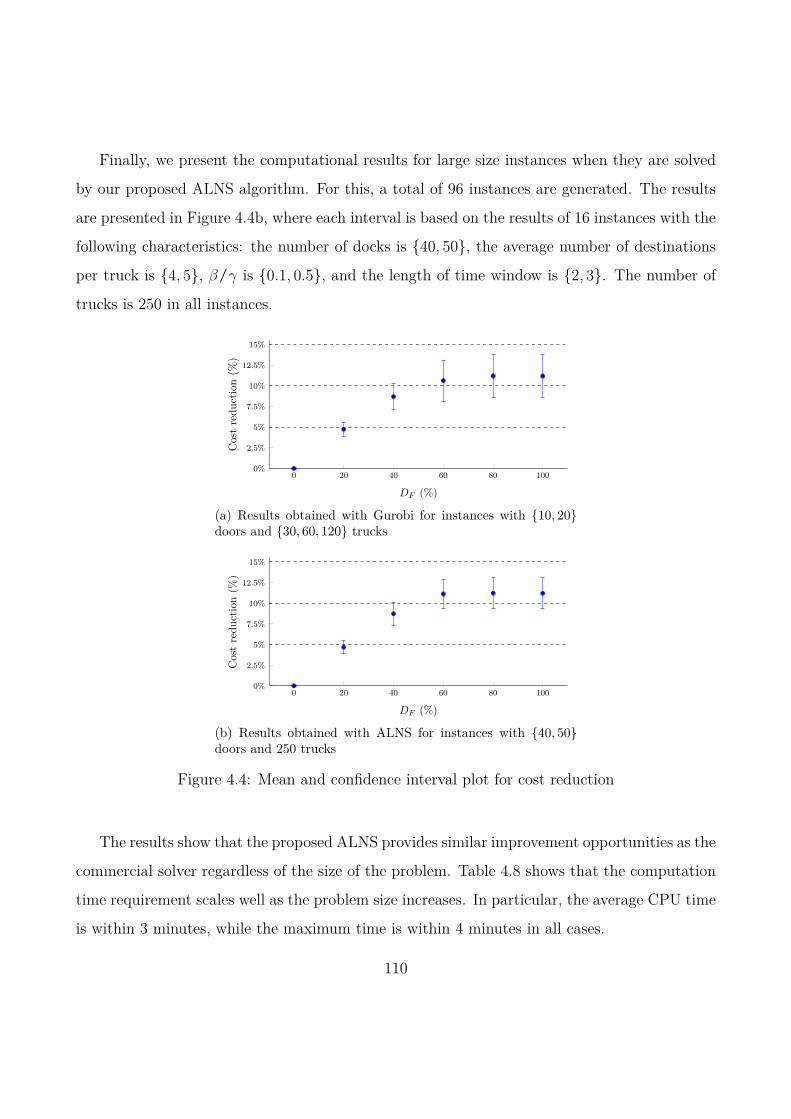
Finally, we present the computational results for large size instances when they are solved
by our proposed ALNS algorithm. For this, a total of 96 instances are generated. The results
are presented in Figure 4.4b, where each interval is based on the results of 16 instances with the
following characteristics: the number of docks is 40, 50, the average number of destinations
per truck is 4, 5, β/γ is 0.1, 0.5, and the length of time window is 2, 3. The number of
trucks is 250 in all instances.
0 20 40 60 80 1000%
2.5%
5%
7.5%
10%
12.5%
15%
DF (%)
Costredu
ction(%
)
(a) Results obtained with Gurobi for instances with 10, 20doors and 30, 60, 120 trucks
0 20 40 60 80 1000%
2.5%
5%
7.5%
10%
12.5%
15%
DF (%)
Costredu
ction(%
)
(b) Results obtained with ALNS for instances with 40, 50doors and 250 trucks
Figure 4.4: Mean and confidence interval plot for cost reduction
The results show that the proposed ALNS provides similar improvement opportunities as the
commercial solver regardless of the size of the problem. Table 4.8 shows that the computation
time requirement scales well as the problem size increases. In particular, the average CPU time
is within 3 minutes, while the maximum time is within 4 minutes in all cases.
110

Table 4.8: CPU time (sec) requirement of ALNS for large size instances with 250 trucks
no. of doors 40 50DF (%) avg max avg max
0 128 174 135 23420 139 200 117 14140 165 212 110 12960 169 211 103 12180 113 131 99 111
100 115 135 101 112
We note that the computation time tends to be shorter as the number of multi-purpose
docks increases. This is due to that as more docks are available to process inbound trucks, a
neighborhood operator is more likely to provide immediately a feasible inbound truck schedule.
Therefore, the time spent to move from one solution to another is reduced.
As a conclusion, the proposed ALNS algorithm is able to solve real size instances within
a reasonable time, providing solutions with a consistent gap when compared to the optimal
solution.
4.7 Conclusions
To the best of our knowledge, this is the first study on truck scheduling in a cross-docking
environment that also shows the effects of operating a set of doors in a mixed mode.
We have presented a model which minimizes the operation costs, i.e., the sum of handling
and tardiness costs. It can be used to find optimal truck schedules for moderate size instances.
We have implemented the model with a commercial solver, Gurobi, and tested the sensitivity of
the solution value to several problem characteristics. The results show that the number of trucks
per dock and the number of destinations per truck are the main factors of the computation
time when searching for an optimal solution.
For larger instances Gurobi cannot provide a solution in a reasonable time, therefore we
propose a heuristic algorithm that follows the principles of the Adaptive Large Neighborhood
111
Search and show that it provides a consistent gap when compared to the best known solution
obtained by the commercial solver. Results show that the computation time requirement of
the proposed heuristic scales well with the problem size.
Our computational results confirm that a few mixed service mode docks can improve the
performance of the cross-dock, as they decrease the total costs. However, the improvement
decreases as the number of mixed service mode docks increases.
112
Bibliography
Agustina, D., C. K. M. Lee, and R. Piplani (2010). A review: Mathematical modles for cross
docking planning. International Journal of Engineering Business Management 2 (2), 47–54.
Ahmadi, R. H. and U. Bagchi (1990). Improved lower bounds for minimizing the sum of
completion times of n jobs over m machines in a flow shop. European Journal of Operational
Research 44 (15), 331–336.
Ahuja, R. K., T. L. Magnanti, and J. B. Orlin (1993). Network Flows: Theory, Algorithms,
and Applications (1 ed.). Prentice Hall: New Jersey.
Akkan, C. and S. Karabatı (2004). The two-machine flowshop total completion time problem:
Improved lower bounds and a branch-and-bound algorithm. European Journal of Operational
Research 159 (2), 420–429.
Alpan, G., A.-L. Ladier, R. Larbi, and B. Penz (2011). Heuristic solutions for transshipment
problems in a multiple door cross docking warehouse. Computers & Industrial Engineer-
ing 61 (2), 402–408.
Alpan, G., R. Larbi, and B. Penz (2011). A bounded dynamic programming approach to
schedule operations in a cross docking platform. Computers & Industrial Engineering 60 (3),
385–396.
Álvarez Pérez, G. A., J. L. González-Velarde, and J. W. Fowler (2009). Crossdocking – Just
in time scheduling: An alternative solution approach. Journal of the Operational Research
Society 60 (60), 554–564.
Ang, M., Y. F. Lim, and M. Sim (2012). Robust storage assignment in unit-load warehouses.
Management Science 58 (11), 2114–2130.
Anken, N., J.-P. Gagliardi, J. Renaud, and A. Ruiz (2011). Space allocation and aisle position-
ing for an industrial pick-to-belt system. Journal of the Operational Research Society 62 (1),
38–49.
Ashayeri, J., L. Gelders, and L. N. Van Wassenhove (1985). A microcomputer-based optimiza-
tion model for the design of automated warehouses. International Journal of Production
Research 23 (4), 825–839.
Ashayeri, J. and L. F. Gelders (1985). Warehouse design optimization. European Journal of
Operational Research 21 (3), 285–294.
Baker, P. and M. Canessa (2009). Warehouse design: A structured approach. European Journal
of Operational Research 193 (2), 425–436.
Bartholdi III, J. J., D. D. Eisenstein, and R. D. Foley (2001). Performance of bucket brigades
when work is stochastic. Operations Research 49 (5), 710–719.
Bartholdi III, J. J. and K. R. Gue (2000). Reducing labor costs in an LTL crossdocking terminal.
Operations Research 48 (6), 823–832.
Bartholdi III, J. J. and K. R. Gue (2004). The best shape for a crossdock. Transportation
Science 38 (2), 235–244.
Bartholdi III, J. J., K. R. Gue, and K. Kang (2008). Staging protocols for unit-load crossdock-
ing. In M. Lahmar (Ed.), Facility Logistics, pp. 153–172. Auerbach Publications.
114
Bassan, Y., Y. Roll, and M. J. Rosenblatt (1980). Internal layout design of a warehouse. AIIE
Transactions 12 (4), 317–322.
Bellanger, A., S. Hanafi, and C. Wilbaut (2013). Three-stage hybrid-flowshop model for cross-
docking. Computers & Operations Research 40 (4), 1109–1121.
Bhaskaran, K. and C. J. Malmborg (1990). Economic tradeoffs in sizing warehouse reserve
storage area. Applied Mathematical Modelling 14 (7), 381–385.
Boloori Arabani, A. R., S. M. T. Fatemi Ghomi, and M. Zandieh (2010). A multi-criteria
cross-docking scheduling with just-in-time approach. The International Journal of Advanced
Manufacturing Technology 49, 741–756.
Boloori Arabani, A. R., S. M. T. Fatemi Ghomi, and M. Zandieh (2011). Meta-heuristics
implementation for scheduling of trucks in a cross-docking system with temporary storage.
Expert Systems with Applications 38 (3), 1964–1979.
Boloori Arabani, A. R., M. Zandieh, and S. M. T. Fatemi Ghomi (2012). A cross-docking
scheduling problem with sub-population multi-objective algorithms. The International Jour-
nal of Advanced Manufacturing Technology 58 (5-8), 741–761.
Boysen, N. (2010). Truck scheduling at zero-inventory cross docking terminals. Computers &
Operations Research 37 (1), 32–41.
Boysen, N. and M. Fliedner (2010). Cross dock scheduling: Classification, literature review
and research agenda. Omega 38 (6), 413–422.
Boysen, N., M. Fliedner, and A. Scholl (2010). Scheduling inbound and outbound trucks at
cross docking terminals. OR Spectrum 32 (1), 135–161.
Briskorn, D., F. Jaehn, and E. Pesch (2013). Exact algorithms for inventory constrained
scheduling on a single machine. Journal of Scheduling 16 (1), 105–115.
115

Brockmann, T. and P. Godin (1997). Flexibility for the future in warehouse design. IIE
Solutions 27 (7), 22–25.
Chan, F. T. S. and V. Kumar (2009). Hybrid TSSA algorithm-based approach to solve
warehouse-scheduling problems. International Journal of Production Research 47 (4), 919–
940.
Chen, F. and C.-Y. Lee (2009). Minimizing the makespan in a two-machine cross-docking flow
shop problem. European Journal of Operational Research 193 (1), 59–72.
Chen, F. and K. Song (2009). Minimizing makespan in two-stage hybrid cross docking schedul-
ing problem. Computers & Operations Research 36 (6), 2066–2073.
Chu, C. (1992). A branch-and-bound algorithm to minimize total flow time with unequal
release dates. Naval Research Logistics 39 (6), 859–875.
Chuang, Y.-F., H.-T. Lee, and Y.-C. Lai (2012). Item-associated cluster assignment model on
storage allocation problems. Computers & Industrial Engineering 63 (4), 1171–1177.
Cormier, G. and E. A. Gunn (1992). A review of warehouse models. European Journal of
Operational Research 58 (1), 3–13.
De Koster, R. B. M., T. Le-Duc, and K. J. Roodbergen (2007). Design and control of warehouse
order picking: A literature review. European Journal of Operational Research 182 (2), 481–
501.
De Koster, R. B. M. and E. S. Van der Poort (1998). Routing orderpickers in a warehouse: A
comparison between optimal and heuristic solutions. IIE Transactions 30 (5), 469–480.
Della Croce, F., M. Ghirardi, and R. Tadei (2002). An improved branch-and-bound algo-
rithm for the two machine total completion time flow shop problem. European Journal of
Operational Research 139 (2), 293–301.
116
Della Croce, F., V. Narayan, and R. Tadei (1996). The two-machine total completion time flow
shop problem. European Journal of Operational Research 90 (2), 227–237.
Forger, G. (1995). UPS starts world’s premiere cross-docking operation. Modern Materials
Handling 50 (13), 36–38.
Framinan, J. M. and R. Leisten (2003). An efficient constructive heuristic for flowtime min-
imisation in permutation flow shops. Omega 31 (4), 311–317.
Framinan, J. M., R. Leisten, and C. Rajendran (2003). Different initial sequences for the
heuristic of Nawaz, Enscore and Ham to minimize makespan, idletime or flowtime in the
static permutation flowshop sequencing problem. International Journal of Production Re-
search 41 (1), 141–148.
Framinan, J. M., R. Leisten, and R. Ruiz-Usano (2005). Comparison of heuristics for flowtime
minimisation in permutation flowshops. Computers & Operations Research 5 (5), 1237–1254.
Francis, R. L. and J. A. White (1992). Facility Layout and Location: An Analytical Approach
(2 ed.). Prentice-Hall, Englewood Cliffs, NJ.
Frazelle, E. H. (2002). World-class warehousing and material handling. McGraw-Hill: New
York.
Frazelle, E. H. and G. P. Sharp (1989). Correlated assignment strategy can improve order-
picking operation. Industrial Engineering 4, 33–37.
Fu, Z., R. Eglese, and L. Y. O. Li (2005). A new tabu search heuristic for the open vehicle
routing problem. Journal of the Operational Research Society 56 (3), 267–274.
Garfinkel, M. (2005). Minimizing multi-zone orders in the correlated storage assignment prob-
lem. Ph.d. thesis, Georgia Institute of Technology.
117

Gharehgozli, A. H., G. Laporte, T. Yu, and R. B. M. De Koster (2013). Scheduling two yard
cranes handling requests with precedences in a container block with multiple open locations.
working paper.
Goetschalckx, M. and J. Ashayeri (1989). Classification and design of order picking systems.
Logistics Information Management 2 (2), 99–106.
Goetschalckx, M. and H. D. Ratliff (1990). Storage policies based on the duration stay of unit
loads. Management Science 36 (9), 1120–1132.
Goh, M., O. Jihong, and T. Chung-Piaw (2001). Warehouse sizing to minimize inventory and
storage costs. Naval Research Logistics 48 (4), 299–312.
Gonzalez, T. and S. Sahni (1978). Flowshop and jobshop schedules: complexity and approxi-
mation. Operations Research 26 (1), 36–52.
Graham, R. L., E. L. Lawler, J. K. Lenstra, and A. H. Rinnooy Kan (1979). Optimization
and approximation in deterministic sequencing and scheduling: a survey. Annals of Discrete
Mathematics 5, 287–326.
Gu, J., M. Goetschalckx, and L. F. McGinnis (2007). Research on warehouse operation: A
comprehensive review. European Journal of Operational Research 177 (1), 1–21.
Gu, J., M. Goetschalckx, and L. F. McGinnis (2010a). Research on warehouse design and
performance evaluation: A comprehensive review. European Journal of Operational Re-
search 203 (3), 539–579.
Gu, J., M. Goetschalckx, and L. F. McGinnis (2010b). Solving the forward-reserve allocation
problem in warehouse order picking systems. Journal of the Operational Research Soci-
ety 61 (6), 1013–1021.
Gue, K. R. (1999). The effects of trailer scheduling on the layout of freight terminals. Trans-
portation Science 33 (4), 419–428.
118

Gue, K. R., G. Ivanovic, and R. D. Meller (2012). A unit-load warehouse with multiple pickup
and deposit points and non-traditional aisles. Transportation Research Part E: Logistics and
Transportation Review 48 (4), 795–806.
Gue, K. R. and R. D. Meller (2009). Aisle configurations for unit-load warehouses. IIE Trans-
actions 41 (3), 171–182.
Hackman, S. T. and L. K. Platzman (1990). Near-optimal solution of generalized resource
allocation problems with large capacities. Operations Research 38 (5), 902–910.
Hackman, S. T., M. J. Rosenblatt, and J. M. Olin (1990). Allocating items to an automated
storage and retrieval system. IIE Transactions 22 (1), 7–14.
Hall, R. W. (1993). Distance approximations for routing manual pickers in a warehouse. IIE
Transactions 25 (4), 76–87.
Hausman, W. H., L. B. Schwarz, and S. C. Graves (1976). Optimal storage assignment in
automatic warehousing systems. Management Science 22 (6), 629–638.
Heragu, S. S., L. Du, R. J. Mantel, and P. C. Schuur (2005). Mathematical model for warehouse
design and product allocation. International Journal of Production Research 43 (2), 327–338.
Heskett, J. (1963). Cube-per-order index – A key to warehouse stock location. Transportation
& Distribution Management 3 (4), 27–31.
Heskett, J. (1964). Putting the cube-per-order index to work in warehouse layout. Transporta-
tion & Distribution Management 4, 23–30.
Hoogeveen, H., L. van Norden, and S. van de Velde (2006). Lower bounds for minimizing total
completion time in a two-machine flow shop. Journal of Scheduling 9 (6), 559–568.
Ignall, E. and L. Schrage (1965). Application of the branch and bound technique to some
flowshop scheduling problems. Operations Research 13 (3), 400–412.
119
Jaikumar, R. and M. Solomon (1990). Dynamic operational policies in an automated warehouse.
IIE Transactions 22 (4), 370–376.
Jane, C.-C. and Y.-W. Laih (2005). A clustering algorithm for item assignment in a synchro-
nized zone order picking system. European Journal of Operational Research 166 (2), 498–496.
Jarvis, J. M. and E. D. McDowell (1991). Optimal product layout in an order picking warehouse.
IIE Transactions 23, 93–102.
Johnson, M. E. and M. L. Brandeau (1996). Stochastic modeling for automated material
handling system design and control. Transportation Science 30 (4), 330–350.
Joustra, P., E. van der Sluis, and N. M. van Dijk (2010). To pool or not to pool in hospitals:
a theoretical and practical comparison for a radiotherapy outpatient department. Annals of
Operations Research 178 (1), 77–89.
Konur, D. and M. M. Golias (2013). Cost-stable truck scheduling at a cross-dock facility
with unknown truck arrivals: A meta-heuristic approach. Transportation Research Part E:
Logistics and Transportation Review 49 (1), 71–91.
Kovács, A. (2011). Optimizing the storage assignment in a warehouse served by milkrun logis-
tics. International Journal of Production Economics 133 (1), 312–318.
Kovacs, A. A., S. N. Parragh, K. F. Doerner, and R. F. Hartl (2012). Adaptive large neigh-
borhood search for service technician routing and scheduling problems. Journal of Schedul-
ing 15 (5), 579–600.
Kulturel, S., N. E. Ozemirel, C. Sepil, and Z. Bozkurt (1999). Experimental investigation of
shared storage assignment policies in automated storage/retrieval systems. IIE Transac-
tions 31 (8), 739–749.
Laha, D. and S. C. Sarin (2009). A heuristic to minimize total flow time in permutation flow
shop. Omega 37 (3), 734–739.
120

Larbi, R., G. Alpan, P. Baptiste, and B. Penz (2011). Scheduling cross docking operations under
full, partial and no information on inbound arrivals. Computers & Operations Research 38,
889–900.
Lee, M.-K. and E. A. Elsayed (2005). Optimization of warehouse storage capacity under a
dedicated storage policy. International Journal of Production Research 43 (9), 1785–1805.
Li, Y., A. Lim, and B. Rodrigues (2004). Crossdocking - JIT scheduling with time windows.
Journal of the Operational Research Society 55 (12), 1342–1351.
Liao, T. W., P. J. Egbelu, and P. C. Chang (2012). Two hybrid differential evolution algorithms
for optimal inbound and outbound truck sequencing in cross docking operations. Applied Soft
Computing 12 (11), 3683–3697.
Liao, T. W., P. J. Egbelu, and P. C. Chang (2013). Simultaneous dock assignment and se-
quencing of inbound trucks under a fixed outbound truck schedule in multi-door cross docking
operations. International Journal of Production Economics 141 (1), 212–229.
Liu, C.-M. (2004). Optimal storage layout and order picking for warehousing. International
Journal of Operations Research 1 (1), 37–46.
Liu, J. and C. R. Reeves (2001). Constructive and composite heuristic solutions to the P//∑Ci
scheduling problem. European Journal of Operational Research 132 (2), 439–452.
Malmborg, C. J. (1996a). An integrated storage system evaluation model. Applied Mathematical
Modelling 20 (5), 359–370.
Malmborg, C. J. (1996b). Storage assignment policy tradeoffs. International Journal of Pro-
duction Research 34 (2), 363–378.
Malmborg, C. J. and K. Bhaskaran (1990). A revised proof of optimality for the cube-per-order
index rule for stored item location. Applied Mathematical Modelling 14 (2), 87–95.
121

Mantel, R. J., P. C. Schuur, and S. S. Heragu (2007). Order oriented slotting: a new assignment
strategy for warehouses. European Journal of Industrial Engineering 1 (3), 301–316.
Matson, J. O. and J. A. White (1982). Operational research and material handling. European
Journal of Operational Research 11 (4), 309–318.
Miao, Z., A. Lim, and H. Ma (2009). Truck dock assignment problem with operational time
constraint within crossdocks. European Journal of Operational Research 192 (1), 105–115.
Muppani, M. V. R. and G. K. Adil (2008a). A branch and bound algorithm for class based
storage location assignment. European Journal of Operational Research 189 (2), 492–507.
Muppani, M. V. R. and G. K. Adil (2008b). Efficient formation of storage classes for warehouse
storage location assignment: A simulated annealing approach. Omega 36 (4), 609–618.
Muralidharan, B., R. J. Linn, and R. Pandit (1995). Shuffling heuristics for the storage location
assignment in an AS/RS. International Journal of Production Research 33 (6), 1661–1673.
Oh, Y., H. Hwang, C. N. Chab, and S. Leec (2006). A dock-door assignment problem for the
Korean mail distribution center. Computers & Industrial Engineering 51 (2), 288–296.
Pan, Q.-K. and R. Ruiz (2013). A comprehensive review and evaluation of permutation flowshop
heuristics to minimize flowtime. Computers & Operations Research 40 (1), 117–128.
Parikh, P. J. and R. D. Meller (2008). Selecting between batch and zone order picking strate-
gies in a distribution center. Transportation Research Part E: Logistics and Transportation
Review 44 (5), 696–719.
Petersen II, C. G. (1999). The impact of routing and storage policies on warehouse efficiency.
International Journal of Operations & Production Management 19 (10), 1053–1064.
Petersen II, C. G. and R. W. Schmenner (1999). An evaluation of routing and volume-based
storage policies in an order picking operation. Decision Sciences 30 (2), 481–501.
122
Pisinger, D. and S. Ropke (2007). A general heuristic for vehicle routing problems. Computers
& Operations Research 34 (8), 2403–2435.
Pliskin, J. S. and D. Dori (1982). Ranking alternative warehouse area assignments: A multi-
attribute approach. IIE Transactions 14 (1), 19–26.
Potts, C. N. and L. N. Van Wassenhove (1983). An algorithm for single machine sequencing
with deadlines to minimize total weighted completion time. European Journal of Operational
Research 12 (12), 379–387.
Rajendran, C. and H. Ziegler (1997). An efficient heuristic for scheduling in a flowshop to
minimize total weighted flowtime of jobs. European Journal of Operational Research 103 (1),
129–138.
Ratliff, H. D. and A. S. Rosenthal (1983). Order-picking in a rectangular warehouse: a solvable
case of the traveling salesman problem. Operations Research 31 (3), 507–521.
Roll, Y. and M. J. Rosenblatt (1983). Random versus grouped storage policies and their effect
on warehouse capacity. Material Flow 1 (3), 199–2005.
Roodbergen, K. J. (2001). Layout and routing method for warehouses. Ph. D. thesis, RSM
Erasmus University, The Netherlands.
Roodbergen, K. J. and I. F. A. Vis (2006). A model for warehouse layout. IIE Transac-
tions 38 (10), 799–811.
Roodbergen, K. J. and I. F. A. Vis (2009). A survey of literature on automated storage and
retrieval systems. European Journal of Operational Research 194 (2), 343–362.
Ropke, S. and D. Pisinger (2006a). An adaptive large neighborhood search heuristic for the
pickup and delivery problem with time windows. Transportation Science 40 (4), 455–472.
123

Ropke, S. and D. Pisinger (2006b). A unified heuristic for a large class of vehicle routing
problems with backhauls. European Journal of Operational Research 171 (3), 750–775.
Rosenblatt, M. J. and A. Eynan (1989). Deriving the optimal boundaries for class-based
automatic storage/retrieval systems. Management Science 35 (12), 1519–1524.
Rosenblatt, M. J. and Y. Roll (1984). Warehouse design with storage policy considerations.
International Journal of Production Research 22 (5), 809–821.
Rouwenhorst, B., B. Reuter, V. Stockrahm, G. J. van Houtum, R. J. Mantel, and W. H. M.
Zijm (2000). Warehouse design and control: Framework and literature review. European
Journal of Operational Research 122 (3), 515–533.
Ruben, R. A. and F. R. Jacobs (1999). Batch construction heuristics and storage assignment
strategies for walk/ride and pick systems. Management Science 45 (4), 575–596.
Saddle Creek Corporation (2011). 2011 cross-docking trends report.
http://www.sclogistics.com/component/content/article/9-uncategorised/150-white-papers.
accessed on 15 November 2012.
Sadiq, M., T. L. Landers, and G. D. Taylor (1996). An assignment algorithm for dynamic
picking systems. IIE Transactions 28 (8), 607–616.
Sadykov, R. (2012). Scheduling incoming and outgoing trucks at cross docking terminals to
minimize the storage cost. Annals of Operations Research 201 (1), 423–440.
Sarker, B. R. and P. S. Babu (1995). Travel time models in automated storage/retrieval systems:
A critical review. International Journal of Production Economics 40 (2–3), 173–185.
Shakeri, M., M. Y. H. Low, S. J. Turner, and E. W. Lee (2012). A robust two-phase heuristic
algorithm for the truck scheduling problem in a resource-constrained crossdock. Computers
& Operations Research 39 (11), 2564–2577.
124
Soltani, R. and S. J. Sadjadi (2010). Scheduling trucks in cross-docking systems: A robust
meta-heuristics approach. Transportation Research Part E: Logistics and Transportation
Review 46 (5), 650–666.
Stalk, G., P. Evans, and S. L. E. (1992). Competing on capabilities: The new role of corporate
strategy. Harvard Business Review 70 (2), 57–69.
Stenger, A., D. Vigo, S. Enz, and M. Schwind (2013). An adaptive variable neighborhood search
algorithm for a vehicle routing problem arising in small package shipping. Transportation
Science 47 (1), 64–80.
Steudel, H. J. (1979). Generating pallet loading patterns: A special case of the two-dimensional
cutting stock problem. Management Science 25 (10), 997–1004.
Taillard, E. (1993). Benchmarks for basic scheduling problems. European Journal of Operational
Research 64 (2), 287–285.
T’kindt, V., F. Della Croce, and C. Esswein (2004). Revisiting branch and bound search
strategies for machine scheduling problems. Journal of Scheduling 7 (6), 429–440.
Tompkins, J. A., J. A. White, Y. A. Bozer, E. H. Frazelle, and J. M. A. Tanchoco (2010).
Facilities Planning (4th ed.). John Wiley & Sons.
Tsai, R. D., E. M. Malstrom, and H. D. Meeks (1988). A two-dimensional palletizing procedure
for warehouse loading operations. IIE Transactions 20 (4), 418–425.
Tsui, L. Y. and C.-H. Chang (1990). A microcomputer based decision support tool for assigning
dock doors in freight yards. Computers & Industrial Engineering 19 (1-4), 309–312.
Tsui, L. Y. and C.-H. Chang (1992). An optimal solution to a dock door assignment problem.
Computers & Industrial Engineering 23 (1-4), 283–286.
125
Vahdani, B. and M. Zandieh (2010). Scheduling trucks in cross-docking systems: Robust
meta-heuristics. Computers & Industrial Engineering 58 (1), 12–24.
Van Belle, J., P. Valckenaers, and D. Cattrysse (2012). Cross-docking: State of the art.
Omega 40 (6), 827–846.
van de Velde, S. L. (1990). Minimizing the sum of the job completion times in the two-machine
flow shop by lagrangian relaxation. Annals of Operations Research 26 (1–4), 257–268.
van den Berg, J. P. (1999). A literature survey on planning and control of warehousing systems.
IIE Transactions 31 (8), 751–762.
van den Berg, J. P., G. P. Sharp, A. J. R. M. (Noud) Gademann, and Y. Pochet (1998).
Forward-reserve allocation in a warehouse with unit-load replenishments. European Journal
of Operational Research 111 (1), 98–113.
van Dijk, N. M. and E. van der Sluis (2008). To pool or not to pool in call centers. Production
and Operations Management 17 (3), 296–305.
Vis, I. F. A. and K. J. Roodbergen (2008). Positioning of goods in a cross-docking environment.
Computers & Industrial Engineering 54 (3), 677–689.
Wäscher, G. (2004). Order picking: A survey of planning problems and methods. In H. Dy-
ckhoff, R. Lackes, and J. Reese (Eds.), Supply Chain Management and Reverse Logistics (1
ed.)., pp. 323–347. Springer.
Witt, C. E. (1998). Crossdocking: Concepts demand choice. Material Handling Engineer-
ing 53 (7), 44–49.
Yan, H. and S.-l. Tang (2009). Pre-distribution and post-distribution cross-docking operations.
Transportation Research Part E: Logistics and Transportation Review 45 (6), 843–859.
126
Yu, W. and P. J. Egbelu (2008). Scheduling of inbound and outbound trucks in cross docking
systems with temporary storage. European Journal of Operational Research 184 (1), 377–396.
Yu, Y. and R. B. M. De Koster (2013). On the suboptimality of full turnover-based storage.
International Journal of Production Research 51 (6), 1635–1647.
127


![PropagationofaThermo-mechanicalPerturbationona ...model (H-H) [1], which considers the action potential as an electrical phe-nomenon induced by the flow of ions through protein channels,](https://static.fdocuments.in/doc/165x107/607da1de621db96070685c70/propagationofathermo-mechanicalperturbationona-model-h-h-1-which-considers.jpg)