Essays on Closed-End Funds and Advance Disclosure of Trading

Essays on Closed-End Funds

and Advance Disclosure of Trading

by

Stephen L. Lenkey

Submitted in partial fulfillment of therequirements for the degree of

Doctor of Philosophyat

Carnegie Mellon UniversityDavid A. Tepper School of Business

Pittsburgh, Pennsylvania

Dissertation Committee:Robert M. Dammon

Jonathan GloverRichard C. Green (chair)

Chester S. Spatt

Spring 2012

Abstract

My dissertation is comprised of three essays. In the first essay, I present a dynamic partial equi-librium model of a simple economy with a closed-end fund. My model demonstrates that a com-bination of management fees and a time-varying information advantage for a fund manager canaccount for several empirically observed characteristics of closed-end funds simultaneously. Themodel is consistent with the basic time-series behavior of fund discounts, explains why funds issueat a premium, accounts for the excess volatility of fund returns, justifies the underperformanceof funds that trade at a premium, and is consistent with many time-series correlations betweendiscounts, NAV returns, and fund returns.

In the second essay, I present a dynamic rational expectations model of closed-end fund discountsthat incorporates feedback effects from activist arbitrage and lifeboat provisions. I find that thepotential for activism and the existence of a lifeboat both lead to narrower discounts. Furthermore,both activist arbitrage and lifeboats effectuate an ex post transfer of wealth from managers toinvestors but an ex ante transfer of wealth from low-ability managers to high-ability managers. Onaverage, investor wealth is unaffected by either activist arbitrage or lifeboats because their potentialbenefits are factored into higher fund prices. Although lifeboats can reduce takeover attempts, theydo not increase expected managerial wealth.

In the third essay, I present a noisy rational expectations equilibrium model in which agents whopossess private information regarding the profitability of a firm are required to provide advance dis-closure of their trading activity. I analytically characterize an equilibrium and conduct a numericalanalysis to evaluate the implications of advance disclosure relative to a market in which informedagents trade without providing advance disclosure. By altering the information environment alongwith managerial incentives, advance disclosure increases risk in the financial market while reducingrisk in the real economy. I also find that advance disclosure has implications for equilibrium pricesand allocations, managerial compensation contracts, investor welfare, and market liquidity.

Contents

1 The Closed-End Fund Puzzle: Management Fees and Private Information 11.1 Introduction . . . . . . . . . . . . . . . . . . . . . . . . . . . . . . . . . . . . . . . . . 11.2 Basic Model . . . . . . . . . . . . . . . . . . . . . . . . . . . . . . . . . . . . . . . . . 5

1.2.1 Equilibrium at t = 3 . . . . . . . . . . . . . . . . . . . . . . . . . . . . . . . . 81.2.2 Equilibrium at t = 2 . . . . . . . . . . . . . . . . . . . . . . . . . . . . . . . . 101.2.3 Equilibrium at t = 1 . . . . . . . . . . . . . . . . . . . . . . . . . . . . . . . . 121.2.4 Implications of the Basic Model . . . . . . . . . . . . . . . . . . . . . . . . . . 14

1.3 Extended Model . . . . . . . . . . . . . . . . . . . . . . . . . . . . . . . . . . . . . . 161.3.1 Assumptions . . . . . . . . . . . . . . . . . . . . . . . . . . . . . . . . . . . . 161.3.2 Equilibrium . . . . . . . . . . . . . . . . . . . . . . . . . . . . . . . . . . . . . 181.3.3 Simulation . . . . . . . . . . . . . . . . . . . . . . . . . . . . . . . . . . . . . 20

1.4 Conclusion . . . . . . . . . . . . . . . . . . . . . . . . . . . . . . . . . . . . . . . . . 28

2 Activist Arbitrage, Lifeboats, and Closed-End Funds 292.1 Introduction . . . . . . . . . . . . . . . . . . . . . . . . . . . . . . . . . . . . . . . . . 292.2 Model . . . . . . . . . . . . . . . . . . . . . . . . . . . . . . . . . . . . . . . . . . . . 32

2.2.1 Benchmark Discount . . . . . . . . . . . . . . . . . . . . . . . . . . . . . . . . 342.2.2 Activist Arbitrage . . . . . . . . . . . . . . . . . . . . . . . . . . . . . . . . . 342.2.3 Lifeboats . . . . . . . . . . . . . . . . . . . . . . . . . . . . . . . . . . . . . . 372.2.4 Combination of Activist Arbitrage and a Lifeboat . . . . . . . . . . . . . . . 39

2.3 Simulation . . . . . . . . . . . . . . . . . . . . . . . . . . . . . . . . . . . . . . . . . . 422.3.1 Benchmark Simulation . . . . . . . . . . . . . . . . . . . . . . . . . . . . . . . 422.3.2 Activist Simulation . . . . . . . . . . . . . . . . . . . . . . . . . . . . . . . . . 432.3.3 Lifeboat Simulation . . . . . . . . . . . . . . . . . . . . . . . . . . . . . . . . 492.3.4 Combined Simulation . . . . . . . . . . . . . . . . . . . . . . . . . . . . . . . 54

2.4 Conclusion . . . . . . . . . . . . . . . . . . . . . . . . . . . . . . . . . . . . . . . . . 59

3 Advance Disclosure of Insider Trading 603.1 Introduction . . . . . . . . . . . . . . . . . . . . . . . . . . . . . . . . . . . . . . . . . 603.2 Model . . . . . . . . . . . . . . . . . . . . . . . . . . . . . . . . . . . . . . . . . . . . 63

3.2.1 No Advance Disclosure of Trading . . . . . . . . . . . . . . . . . . . . . . . . 653.2.2 Advance Disclosure of Trading . . . . . . . . . . . . . . . . . . . . . . . . . . 70

3.3 Simulation . . . . . . . . . . . . . . . . . . . . . . . . . . . . . . . . . . . . . . . . . . 753.3.1 Market Efficiency . . . . . . . . . . . . . . . . . . . . . . . . . . . . . . . . . . 773.3.2 Price . . . . . . . . . . . . . . . . . . . . . . . . . . . . . . . . . . . . . . . . . 783.3.3 Risk Premium . . . . . . . . . . . . . . . . . . . . . . . . . . . . . . . . . . . 793.3.4 Liquidity . . . . . . . . . . . . . . . . . . . . . . . . . . . . . . . . . . . . . . 79

i

3.3.5 Allocations . . . . . . . . . . . . . . . . . . . . . . . . . . . . . . . . . . . . . 813.3.6 Trading Profits . . . . . . . . . . . . . . . . . . . . . . . . . . . . . . . . . . . 843.3.7 Welfare . . . . . . . . . . . . . . . . . . . . . . . . . . . . . . . . . . . . . . . 843.3.8 Managerial Effort . . . . . . . . . . . . . . . . . . . . . . . . . . . . . . . . . . 853.3.9 Incentive to Undertake Excessive Risk . . . . . . . . . . . . . . . . . . . . . . 853.3.10 Voluntary Disclosure . . . . . . . . . . . . . . . . . . . . . . . . . . . . . . . . 873.3.11 Sensitivity of Results . . . . . . . . . . . . . . . . . . . . . . . . . . . . . . . . 87

3.4 Concluding Remarks . . . . . . . . . . . . . . . . . . . . . . . . . . . . . . . . . . . . 88

A The Closed-End Fund Puzzle: Management Fees and Private Information 90A.1 Endogenous Stock Price without Liquidity Traders . . . . . . . . . . . . . . . . . . . 90A.2 Endogenous Stock Price with Liquidity Traders . . . . . . . . . . . . . . . . . . . . . 92

B Activist Arbitrage, Lifeboats, and Closed-End Funds 97B.1 Discounts and Parameter Values . . . . . . . . . . . . . . . . . . . . . . . . . . . . . 97B.2 Proofs . . . . . . . . . . . . . . . . . . . . . . . . . . . . . . . . . . . . . . . . . . . . 99

C Advance Disclosure of Insider Trading 103

ii

Chapter 1

The Closed-End Fund Puzzle:Management Fees and PrivateInformation

We present a dynamic partial equilibrium model of a simple economy with a closed-end fund.Our model demonstrates that a combination of management fees and a time-varying informationadvantage for a fund manager can account for several empirically observed characteristics of closed-end funds simultaneously. The model is consistent with the basic time-series behavior of funddiscounts, explains why funds issue at a premium, accounts for the excess volatility of fund returns,justifies the underperformance of funds that trade at a premium, and is consistent with manytime-series correlations between discounts, NAV returns, and fund returns.

1.1 Introduction

For more than four decades, economists have struggled to understand the perplexing behaviorsexhibited by closed-end fund prices. These behaviors, which over the years have become knowncollectively as the closed-end fund puzzle, are baffling on a number of levels. The most well-knownfeature of the puzzle is that a closed-end fund’s discount, or the difference between the price ofthe fund’s shares and its net asset value (NAV), tends to follow a predictable pattern over thefund’s life cycle. There are, however, several aspects of the closed-end fund puzzle in addition tothe basic time-series properties of discounts that are equally intriguing and important. One suchaspect is that the returns on a fund’s shares tend to be more volatile than the returns on the fund’sunderlying assets. If closed-end funds are merely a portfolio of assets, why are fund prices morevolatile than the underlying assets? This question is especially fascinating in light of the fact thatfund prices underreact to NAV returns. Another feature of the puzzle is that funds that trade ata premium tend to underperform relative to those that trade at a discount. This raises an obviousquestion: why do investors buy funds at a premium when they expect them to underperform?Furthermore, many of the correlations between the time-series of discounts, NAV returns, and fundreturns appear to defy common sense. For example, why are discounts correlated with future fundreturns but not future NAV returns? We address all of these features of the closed-end fund puzzlein this paper.

While numerous frictions have been suggested over the years as the basis for the behavior ofclosed-end fund prices, we demonstrate that a model combining two fundamental elements canexplain most of the salient facts about closed-end funds simultaneously: (i) a time-varying infor-

1

mation advantage for a fund manager; and (ii) management fees. More specifically, we propose adynamic partial equilibrium model in which a closed-end fund manager periodically acquires privateinformation regarding the future performance of an underlying asset.1 The manager then exploitsher time-varying information advantage to earn positive abnormal returns for the fund prior todeducting management fees. Whether a fund trades at a discount or a premium depends on thevalue of the manager’s information in relation to the fees she collects for managing the fund.

Because a closed-end fund issues a fixed number of nonredeemable shares that trade at a pricedetermined by the market, the price of a fund’s shares often diverges from the fund’s NAV in anapparent violation of the Law of One Price. In fact, closed-end fund discounts tend to follow apredictable pattern over a fund’s life cycle, as documented by Lee, Shleifer, and Thaler (1990) andothers. Consistent with this well-documented time-series behavior of discounts, funds in our modelissue at a premium when the expected benefit from the manager’s information advantage outweighsthe cost of the management fees. After the manager’s private information is exploited, however,funds begin to trade at a discount because the capitalized future management fees outweigh theexpected benefits from the manager’s future information advantages. The rapid emergence of a dis-count in our model is consistent with existing empirical studies by Weiss (1989) and Peavy (1990)who find that funds usually begin to trade at a discount within 100 days following the initial pub-lic offering (IPO). Furthermore, the time-varying nature of the manager’s information advantageleads to both cross-sectional and time-series fluctuations in discounts. Lastly, fund prices in ourmodel converge to a fund’s NAV when the fund is terminated, which is consistent with empiricalevidence that prices converge to NAV when funds are liquidated (Brickley and Schallheim (1985))or reorganized into an open-end mutual fund (Brauer (1984)).

In addition to accounting for the basic time-series behavior of discounts over a fund’s life cycle,our model also explains why funds issue at a premium. According to our model, funds issue at apremium because issue premiums are utility-maximizing for fund managers, and investors are will-ing to pay a premium because doing so maximizes their own expected utility and clears the market.The driving force behind this result is the management fee, which simultaneously impacts bothmanagerial wealth and the manager’s incentive to exploit her information advantage by selectingthe fund’s portfolio of underlying assets. It turns out that the size of the fee that maximizes therisk-averse manager’s expected utility also maximizes the value of the fund for investors becausethe fee influences how aggressively the manager trades on her private information.

Our model also accounts for the excess volatility of fund returns despite the fact that fundprices underreact to NAV returns, as reported by Pontiff (1997). Consistent with empirical obser-vations, fund returns in our model are more volatile than NAV returns but covary negatively withchanges in premiums. Moreover, the fundamental source of a fund’s excess volatility in our modelis the manager’s information advantage, which is consistent with empirical evidence that marketrisk factors do not explain excess volatility.

We also demonstrate that a combination of management fees and a time-varying informationadvantage for a fund manager can justify one of the most anomalous characteristics of closed-endfunds—the underperformance of funds that trade at a premium relative to those that trade at adiscount, which has been documented by Thompson (1978) and Pontiff (1995). Funds that tradeat a premium in our model tend to underperform because they provide insurance against extremereturns of the underlying assets. In our model, funds trade at a premium only when the managerpossesses a large information advantage, but possessing a large quantity of private information gen-

1Our use of the term “private information” should be broadly construed as the ability to more accurately predictfuture prices. While we do not rule out the possibility of a fund manager trading on “insider” information, a manager’sinformation advantage could stem from, say, a skill set specially tailored to a particular economic environment. Wediscuss potential sources of the manager’s information advantage in more detail in Section 1.3.1.

2

erates a large abnormal return only in the relatively rare instances where the private informationindicates that there will be an extreme return for an underlying asset. In these rare cases, themanager can modify the fund’s portfolio to capitalize on her information advantage and therebygenerate a large abnormal return for the fund. Most of the time, however, the underlying assets willnot produce an extreme return. In these cases, which occur with great frequency, the manager’scapability to earn a large abnormal return net of management fees is greatly diminished becauseher private information is not very valuable. As a result, funds that trade at a premium tend tounderperform on average. Nevertheless, risk-averse investors are willing to hold such funds eventhough they expect them to underperform since those funds protect investors from extreme losses.

Finally, our model is consistent with many of the time-series correlations between discounts,NAV returns, and fund returns. Discounts in our model are persistent over time, are unrelatedto both past and future NAV returns, and are positively correlated with future fund returns butnegatively correlated with lagged fund returns. Additionally, NAV returns and fund returns arenot perfectly correlated.

In light of the fact that there is conflicting empirical evidence regarding both the existence ofmanagerial ability and the impact of management fees on discounts, the appropriateness of model-ing the source of the puzzling behaviors exhibited by closed-end fund prices as a tradeoff betweena time-varying information advantage for a fund manager and management fees warrants furtherdiscussion. Intuitively, it seems like management fees should affect discounts because on some levelfees represent a dead weight cost to a fund’s shareholders. In line with this reasoning, Kumarand Noronha (1992) and Johnson, Lin, and Song (2006) report that discounts are significantlyand positively related to fund expenses. At the same time, empirical studies by Malkiel (1977)and Barclay, Holderness, and Pontiff (1993) indicate that management fees do not significantlycontribute to observed discounts. Our model provides a novel explanation for this conflicting em-pirical evidence, although a few arguments have previously emerged in the literature to reconcileour intuition with the facts.2 In our model, the relationship between the management fee andthe discount is nonlinear and non-monotonic because the size of the fee determines not only theamount of wealth transferred from investors to the manager but also influences how aggressivelythe manager trades on her private information. Since the degree to which the manager exploitsher information advantage affects the value of the fund in a nonlinear and non-monotone fashion,it is not surprising that empirical studies have generated mixed evidence concerning the effect ofmanagement fees on discounts.

The empirical evidence regarding the existence of managerial ability is conflicted, as well. Inrecent work, Fama and French (2010) report that open-end mutual fund managers add little valueover the long term. Once management fees are taken into account, managers seem to producenegative abnormal returns on average. On the other hand, Chay and Trzcinka (1999) find thatclosed-end fund premiums are positively related to future managerial performance over the shortterm but not the long term. Our model is not inconsistent with either of these studies. Mostof the time, the fund manager in our model generates small positive abnormal returns. Theseabnormal returns become negative after deducting management fees, however, which is why fundsusually trade at a discount. Nevertheless, in the relatively rare instances when the fund trades at apremium, the manager can generate large but short-lived gross abnormal returns. Managerial per-

2One explanation by Gemmill and Thomas (2002) is that management fees frequently show up as being insignif-icantly related to discounts in reduced form empirical studies because fees are highly collinear with other variablesthat affect closed-end fund discounts. Another explanation by Chay and Trzcinka (1999) is that reported fees do notinclude soft dollar expenses. Alternatively, Deaves and Krinsky (1994) argue that higher fees increase the probabilityof a takeover attempt, which in turn results in lower discounts due to the price feedback effect created by the potentialtakeover.

3

formance is not persistent because the manager’s information advantages dissipate rather quickly.To our knowledge, our model is the first to simultaneously explain most of the prominent styl-

ized facts about closed-end funds. Other theorists have made some progress in explaining the basictime-series behavior of discounts in recent years, but none have successfully explained the excessvolatility of fund returns, the underperformance of funds that trade at a premium, or the severaltime-series correlations between discounts and returns. For instance, Berk and Stanton (2007)model a tradeoff between a reduced form managerial ability and management fees. By allowing amanager with high ability to extract the surplus she creates via a pay raise, their model is ableto account for the predictable time-series pattern exhibited by discounts over a fund’s life cycle.Additionally, Cherkes, Sagi, and Stanton (2009) demonstrate that liquidity concerns can lead tonew funds issuing at a premium during times when seasoned funds are trading at a premium andthen subsequently falling into a discount, but their model is unable to explain the behavior of dis-counts for funds that hold liquid assets. In contrast to these theories, our model explains not onlythe time-series behavior of discounts but also the excess volatility of fund returns, the underperfor-mance of premium funds, and many of the time-series correlations between discounts and returns.

While the source of divergence between the price of a closed-end fund and its NAV has provento be elusive, we are not the first to surmise that an information advantage of some sort may bethe driving force behind the puzzling behavior of closed-end fund discounts. For example, Oh andRoss (1994) construct an equilibrium model based on an information asymmetry between a fundmanager and investor. They show that the precision of the manager’s private information canimpact a fund’s discount, but since trading takes place at only a single date in their model, it isunable to explain even the time-series properties of discounts, let alone the many other aspects ofthe closed-end fund puzzle. Similarly, Arora, Ju, and Ou-Yang (2003) propose a two-period modelin which the fund manager has an initial information advantage but is constrained by contractuallyimposed investment restrictions. They numerically show that the fund can issue at a premium andlater trade at a discount, but their model does not explain either the cross-sectional or time-seriesvariation in discounts.

The other basic building block of our model, management fees, has also previously been pro-posed as a source of discounts. Ross (2002a) demonstrates that a closed-end fund will trade at adiscount equal to the capitalized management fees if the manager receives a constant percentageof the fund’s NAV in perpetuity. This simple model, however, fails to explain why funds issue ata premium or why discounts fluctuate over time. In related work, Ross (2002b) explores varia-tions of the model and shows that with asymmetrically-informed investors funds may issue at apremium and that dynamic distribution policies can result in a fluctuating discount. Nevertheless,he does not simultaneously model both issue premiums and fluctuating discounts. In contrast toRoss (2002a) and Ross (2002b), our model can explain the time-series attributes of funds withoutrelying on a dynamic distribution policy or information asymmetry among investors at the time ofissuance.3 Our model also accounts for the other prominent aspects of the closed-end fund puzzle.

Several other explanations for the behavior of closed-end fund discounts have been proposedwith varying degrees of success. For example, taxes may provide a partial explanation for theexistence of discounts. Since investors who purchase a closed-end fund with unrealized capital ap-preciation face a future tax liability, the shares of such a fund should trade at a price lower thanan equivalent fund with no unrealized capital appreciation. Malkiel (1977) finds some empiricalsupport for this argument, but he demonstrates that taxes alone cannot quantitatively account for

3The information asymmetry in our model arises after the IPO and is between the fund manager and the investor.Although this may seem like a minor distinction, our model illustrates that contemporaneous asymmetric informationamong investors is not necessary to produce a premium at the IPO or a subsequent discount because only investors,who always have identical information sets, trade shares in the fund.

4

the observed discounts. Kim (1994) argues that tax-timing options also contribute to discounts. Onthe other hand, Brickley, Manaster, and Schallheim (1991) observe a negative correlation betweenunrealized capital appreciation and the discount, which is inconsistent with the taxation argument.Still, taxes do not explain why funds issue at a premium or why the price converges to NAV upontermination.

Malkiel (1977) provides some empirical evidence that funds investing in restricted stocks ex-perience deeper discounts. Similarly, Bonser-Neal, Brauer, Neal, and Wheatley (1990) and Chan,Jain, and Xia (2005) find that international barriers can affect discounts of funds that hold foreignassets, but Kumar and Noronha (1992) find that holding a portfolio of foreign stock does not nec-essarily impact the discount. Nonetheless, investing in restricted or foreign assets does not explaindiscount dynamics for funds that hold liquid domestic assets. Agency costs also have been exploredas a potential factor affecting discounts. Barclay, Holderness, and Pontiff (1993) find that fundswith concentrated block ownership tend to have larger discounts, which they attribute to managersdiverting fund resources for their own private benefit. However, agency costs do not explain thebasic time-series pattern of fund discounts.

Lastly, De Long, Shleifer, Summers, and Waldmann (1990) speculate that the existence of ir-rational noise traders creates additional risk for rational investors with a short investment horizonand results in a lower price for closed-end funds. This theory predicts that new funds will issue ata premium when noise traders are overly optimistic about future performance and that discountswill vary with the fluctuations in noise trader opinion, or investor sentiment. Lee, Shleifer, andThaler (1991) find empirical support for this hypothesis by conjecturing that the investor sentimentdriving closed-end fund discounts also affects stock prices of small firms since individual investors,who are the source of noise-trader risk, are the predominant holders of both types of assets in theU.S. However, Dimson and Minio-Kozerski (1999) note that closed-end funds in the U.K. are pre-dominantly held by institutions but nevertheless tend to trade at a discount. Furthermore, Chan,Jain, and Xia (2005) find that noise traders are not a significant contributor to fund discounts.Other studies have produced mixed evidence in support of the investor sentiment hypothesis (see,e.g., Chen, Kan, and Miller (1993), Chopra, Lee, Shleifer, and Thaler (1993) and Elton, Gruber,and Busse (1998)).

The remainder of this article is organized as follows. In Section 1.2, we outline the basic featuresof the model and solve for the equilibrium over a short time horizon using symbolic computationalmethods. We then demonstrate that our basic model with a short time horizon can account for thepredictable pattern of discounts over a fund’s life cycle and explain why funds issue at a premium.In Section 1.3, we extend the model to a longer time horizon using the techniques discussed inSection 1.2. We then simulate data and assess the model’s ability to account for several empiricalobservations reported in the literature; namely, the puzzling time-series correlations between dis-counts and returns, the excess volatility of fund returns, and the underperformance of funds thattrade at a premium. Finally, Section 1.4 concludes.

1.2 Basic Model

Time is discrete and indexed by t ∈ {1, 2, 3, 4}. Trading in the financial market occurs att = 1, 2, 3 while consumption occurs at t = 4. A single fund manager (she) and a single represen-tative investor (he) are present in the market. Both agents exhibit preferences, which are commonknowledge, characterized by constant absolute risk aversion (CARA), where γi and γm denote thecoefficients of risk aversion for the investor and manager, respectively.

The economy consists of three types of financial assets—a stock, a sequence of one-period bonds,

5

and a closed-end fund. The stock pays a random amount, Y , at t = 4 but does not pay any divi-dends prior to that time. The stock payoff consists of the sum of three independent and normallydistributed random variables,

Y ≡ X1 + X2 + X3, (1.1)

where Xt ∼ N(µt, σ

2t

)for t = 1, 2, 3. As discussed in greater detail below, the value of each Xt

is initially unknown but is observed as time progresses. For simplicity, we assume that the stockprice follows an exogenous process given by

P st =t−1∑τ=1

Xτ +3∑τ=t

(µτ −

γiγmΓ

σ2τ

), (1.2)

where Γ ≡ γi + γm. Hence, the price at time t is equal to the conditional expectation of the stock’spayoff less an adjustment for risk. While the specific form of the exogenous price process is notterribly important for our analysis, this particular process is reflective of endogenous equilibriumprices in models with symmetrically-informed agents who have CARA preferences. Alternatively,the stock price can be determined endogenously within our framework without affecting the fun-damental nature of our analysis. Details of the analysis of our model with endogenous stock pricesare contained in Appendices A.1 and A.2.

A couple of simplifying assumptions are made regarding the bonds. Each one-period bond hasa constant interest rate that is normalized to zero; accordingly, a bond costs one unit at time tand pays one unit at t + 1. Additionally, the supply of each one-period bond is elastic. Theseassumptions dramatically improve the tractability and computational efficiency of the model. Al-though a non-zero interest rate would impact the prices of the stock and closed-end fund, empiricalstudies have found that neither the short-term interest rate (Coles, Suay, and Woodbury (2000))nor changes in interest rates (Gemmill and Thomas (2002) and Lee, Shleifer, and Thaler (1991))significantly affect discounts.

The closed-end fund is an endogenous, time-varying portfolio of the stock and bond. Thisrelatively simple setup highlights the effect of asymmetric information on the discount, though inreality closed-end funds typically specialize in a diversified portfolio of either stocks or bonds (see,e.g., Dimson and Minio-Kozerski (1999)). The fund, whose shares are traded in the market, is inunit supply, and the equilibrium price at time t is endogenous and denoted by P ft . At t = 1, thefund undergoes an IPO. The fund is liquidated at t = 4, and its assets are distributed to the fund’sshareholders at that time after deducting management fees. Furthermore, the fund is prohibitedfrom issuing new shares or repurchasing existing shares. Although the potential for early liquidationor open-ending can impact the discount (see Brauer (1988), Deaves and Krinsky (1994), Gemmilland Thomas (2002), Johnson, Lin, and Song (2006), Bradley et al. (2010), and Lenkey (2011)), weassume that the fund will not be liquidated prior to t = 4 with certainty.

At each trading date, the fund manager chooses the composition of the closed-end fund accord-ing to her preferences by allocating the fund’s financial resources among the bond and stock whilethe investor optimally allocates his wealth across the bond, stock, and fund. At t = 1, the investorreceives an exogenous endowment of wealth, Wi, and he observes the fund’s initial wealth thatis designated for investment, Wf , which is usually reported in a fund’s prospectus. As is typicalin practice, the investor is unable to observe the contemporaneous composition of the fund, buthe acquires knowledge of the prior period composition as time progresses; that is, at time t theinvestor has knowledge of all fund portfolios through t − 1. In some cases, the investor can inferthe fund’s portfolio at the current date based on the fund’s prior portfolios in addition to the other

6

parameters and state variables.4

The fund manager obtains utility solely from the consumption, cm, of fees, φ, earned frommanaging the closed-end fund plus any issue premium, ρ. The management contract is exogenousand pays the manager a fixed amount, a, plus a fraction, b, of the fund’s NAV return,5

φ = a+ b(Sf3 Y +Bf

3 − V1

), (1.3)

where Sft and Bft denote the quantity of stock and number of bonds held by the fund from time t

to t+ 1 andVt ≡ Sft P st +Bf

t (1.4)

denotes the fund’s time-t NAV, which is equal to the market value of the assets in the fund’sportfolio. The initial NAV equals the fund’s initial wealth designated for investment: V1 = Wf .The fund’s time-t discount, Dt, is defined as the difference between the price of the fund and NAV,

Dt ≡ Vt − P ft , (1.5)

which means that the fund’s issue premium is

ρ ≡ P f1 − V1. (1.6)

Defining the discount as the simple difference, as opposed to the more conventional definition ofpercentage or log difference, between the price of the fund and its NAV results in simpler expressionsfor the discount. Percentage and log discounts can easily be obtained from Dt.

The investor, meanwhile, receives utility solely from the consumption, ci, of the payoff from hisportfolio. Hence,

ci = Si3Y +Bi3 + F3

(Sf3 Y +Bf

3 − φ), (1.7)

where Sit denotes the quantity of stock, Bit denotes the number of bonds, and Ft denotes the shares

of the fund held by the investor from time t to t+ 1.Information regarding the stock payoff, Y , evolves over time. Recall that trading in the financial

market occurs at t = 1, 2, 3 and consumption occurs at t = 4. As time progresses, the managerobtains an information advantage over the investor which she exploits to earn an excess return forthe fund. Let Iit and Ift denote the information set at time t for the investor and fund manager,respectively. Initially, the value of each Xt is unknown to both the investor and manager: Ii1 =If1 = ∅. At t = 2, both the manager and investor observe X1. Additionally, the manager observesa portion of X2, and it is at this point that the manager can exploit her information advantage toearn an excess return. We assume that the portion of X2 observed by the fund manager depends on

4Knowledge of prior fund compositions is a sufficient, but not a necessary, condition for the investor to be ableto infer the fund’s current composition when information is symmetric. The investor can still infer the fund’scontemporaneous portfolio when information is symmetric if he instead only observes current NAV.

5This contractual form differs from most compensation contracts in the industry which pay the fund manager afraction of the total assets under management. While the results of the basic model developed in this section arerobust to these more prevalent contractual forms, the “two-part” contract produces more realistic solutions to theextended model presented in Section 1.3. In the extended model, the manager is compensated with a sequence offees over a longer time horizon. If the compensation contract paid the manager a fraction of the total assets undermanagement so that each fee depended on the NAV at a particular date, then portfolio choices would affect not onlythe contemporaneous fee but also all future fees. Hence, such a contract effectively makes holding stock riskier forthe manager than when she is compensated via the two-part contract. Because she has CARA preferences, to offsetthe increased risk the manager would tend to allocate a small amount of the fund’s wealth to the stock at early datesand gradually increase the allocation over time. In contrast, the two-part contract leads to stock allocations that arestationary, which is more realistic.

7

her ability, α ∈ (0, 1), to acquire information, with larger values of α representing a greater ability.Both the manager and investor are able to discern the value of α before the fund undergoes theIPO. We specifically assume that X2 is the sum of two components,

X2 ≡ Z1 + Z2, (1.8)

and that the manager privately observes Z1. Furthermore, we assume that Z1 ∼ N(αµ2, ασ

22

)and Z2 ∼ N

((1 − α)µ2, (1 − α)σ2

2

), which means that the distribution of the stock payoff, Y ,

is independent of ability, yet a manager with a higher ability level acquires more informationthan a manager with low ability. Consequently, the information sets at t = 2 are asymmetric:Ii2 = {X1} and If2 = {X1, Z1}. At t = 3, both agents observe X2, so the information sets areonce again symmetric: Ii3 = If3 = {X1, X2}. Finally, all information is available at the terminaldate: Ii4 = If4 = {X1, X2, X3}. This information structure enables the study of equilibriumdynamics and, in particular, the impact of an information advantage on the closed-end fund price.All acquisition of information is costless; consequently, potential moral hazard issues relating toinformation acquisition do not arise.

The sequence of events is as follows. The fund undergoes an IPO at t = 1, and the investor andmanager subsequently choose portfolios at market-clearing prices. The investor allocates his wealthamong the bond, stock, and fund while the manager allocates the fund’s financial resources amongthe bond and stock. Because preferences are common knowledge and information is symmetric,the investor can infer the fund’s portfolio composition from the equilibrium stock price. At t = 2,the fund discloses its portfolio holdings from the previous date, the manager acquires privateinformation regarding the terminal payoff of the stock, and both the investor and manager rebalancetheir respective portfolios. The investor cannot infer the precise composition of the fund’s currentportfolio since he does not observe Z1, although he does form beliefs about a distribution of thefund’s portfolio based on the manager’s preferences. At t = 3, the fund manager’s informationadvantage disappears, both agents rebalance their respective portfolios, and the investor can onceagain infer the fund’s portfolio from the equilibrium stock price and the composition of the fund’sportfolio from the previous date, which is announced prior to trading. Finally, the managementfees are paid, the portfolios are liquidated, and consumption occurs at t = 4.

We make one final technical assumption regarding the relative magnitudes of the agents’ riskaversion coefficients to ensure well-defined and meaningful solutions: Γb > γi. This assumption isentirely reasonable if γm � γi, which is not unrealistic since in actuality the mass of investors is farlarger than that of fund managers and the coefficients of risk aversion are equivalent to the inversesof the agents’ risk tolerances. In other words, this is an assumption about the relative masses ofthe agents rather than their risk preferences.

The equilibrium is solved recursively with the aid of symbolic computational methods. Section1.2.1 characterizes the equilibrium at t = 3. Those results are then drawn on in Section 1.2.2 toderive the equilibrium at t = 2, which in turn is relied upon to characterize the equilibrium at t = 1in Section 1.2.3. Some implications of the basic model are discussed in Section 1.2.4.

1.2.1 Equilibrium at t = 3

Information is symmetric at t = 3. The equilibrium price of the closed-end fund is derivedfrom the utility-maximizing objectives of the manager and investor. The following propositioncharacterizes the equilibrium discount.

Proposition 1. At t = 3, there exists a unique equilibrium in which the closed-end fund discountis given by

D3 = a+ b(V3 − V1

). (1.9)

8

The remaining portion of this subsection describes the equilibrium derivation, beginning withthe fund manager’s objective. The fund manager’s goal at t = 3 is to maximize her expected utilityfrom consumption of the management fees and issue premium by choosing the composition of theclosed-end fund subject to a budget constraint:

maxSf3

E3

[− exp[−γmcm] |X1, X2

](1.10)

subject to

cm = φ+ ρ (1.11)

Bf3 =

(Sf2 − S

f3

)P s3 +Bf

2 , (1.12)

where Et is the expectation operator conditional on information available at time t. Since, condi-tional on X1 and X2, the manager’s consumption is log-normally distributed, her expected utilitycan be rewritten in closed form as

− exp[−γm

(ρ+ a+ b

[Sf3(X1 +X2 + µ3 − P s3

)+ Sf2P

s3 +Bf

2 − V1

]− 1

2γmb2(Sf3)2σ2

3

)](1.13)

after substituting (1.1), (1.3), (1.11), and (1.12) into (1.10) and integrating over X3. The manager’sstock allocation is then derived by differentiating (1.13) with respect to Sf3 and substituting thestock price, (1.2), into the corresponding first-order condition to obtain

Sf3 =γiΓb. (1.14)

The investor faces a problem similar to that of the manager. The investor’s objective is tomaximize his expected utility from consumption of the assets in his portfolio subject to a budgetconstraint, taking into account the portfolio held by the fund:6

maxSi3, F3

E3

[− exp[−γici] |X1, X2

](1.15)

subject toBi

3 =(Si2 − Si3

)P s3 +Bi

2 +(F2 − F3

)P f3 (1.16)

as well as (1.12) and (1.14). Since the investor’s consumption is also conditionally log-normallydistributed, his expected utility can be rewritten as

− exp[−γi

(Si3(X1 +X2 + µ3 − P s3

)+ Si2P

s3 +Bi

2 + F2Pf3 − 1

2γi(Si3 + (1− b)F3S

f3

)2σ2

3

+ F3

[(1− b)

(Sf3(X1 +X2 + µ3 − P s3

)+ Sf2P

s3 +Bf

2

)+ bV1 − P f3 − a

])](1.17)

after substituting (1.1), (1.3), (1.7), (1.12), and (1.16) into (1.15) and integrating over X3. Differ-entiating (1.17) with respect to Si3 and substituting (1.2) and (1.14) into the first-order conditionprovides the investor’s stock allocation,

Si3 =Γb− γi

Γb. (1.18)

6Recall that the investor can infer the fund’s portfolio at t = 3 since he has knowledge of the prior composition ofthe fund in addition to the other state variables and parameters.

9

Finally, the fund price is obtained by differentiating the investor’s expected utility, (1.17), withrespect to F3 and substituting the stock price, stock allocations, and market-clearing condition(F3 = 1) into the first-order condition, which gives

P f3 = V3 − a− b(V3 − V1

). (1.19)

Thus, the fund price is equal to the fund’s NAV minus an adjustment for the management fees.It follows immediately from (1.19) that the discount, which is given by (1.9), stems from themanagement fees when the investor and manager have identical information sets and there is nopossibility of a future information asymmetry. The fund will trade at a discount (as opposed to apremium) whenever a+ bV3 > bV1; that is to say, appreciation of the NAV is a sufficient conditionfor the fund to trade at a discount.

Since the closed-end fund generally trades at a price different from its NAV, it is conceivablethat an arbitrage opportunity exists. We show here, however, that the discount does not present anarbitrage opportunity. If the fund is trading at a discount relative to NAV, then a potential arbitragestrategy would entail purchasing shares in the fund and simultaneously taking an offsetting positionin a hedging portfolio. Since the fund payoff at t = 4, net of management fees, is

(1− b)(Sf3 Y +Bf

3

)+ bV1 − a,

an appropriate hedging portfolio would consist of −((1 − b)Bf

3 + bV1 − a)

bonds and −(1 − b)Sf3shares of stock, but because the cost of this hedging portfolio equals −P f3 , there is no arbitrageopportunity. In other words, arbitrage does not exist because the discount at t = 3 arises solelyfrom the future management fees, which also reduce the fund payoff.


The stock allocations and equilibrium fund price derived in Section 1.2.1 are used to determinethe equilibrium fund price at t = 2. Recall that information is asymmetric at t = 2 as the fundmanager observes the value of Z1 but the investor does not. The following proposition characterizesthe equilibrium in the presence of asymmetric information.


D2 = a+ b(V2 − V1

)− λ (1.20)

whereλ ≡ α(1− b)(Γb− γi)

α(1− b)γi(Γb− γi + γmb) + (1− α)γ2mb

2. (1.21)

The derivation of the equilibrium is described in the remaining portion of this subsection. Sincethe manager’s expected utility is independent of the investor’s portfolio, the manager’s problem isrelatively straightforward and is analogous to her problem at t = 3. On the other hand, becausethe investor does not observe the manager’s private information, his situation is more complicatedand involves additional uncertainty.

At t = 2, the manager chooses the fund allocation to maximize her expected utility subject toa budget constraint, bearing in mind the future stock price and fund portfolio:

maxSf2

E2

[− exp

[−γm

(ρ + a + b

[γiγmΓ Sf3σ

23 + Sf2 P

s3 + Bf

2 − V1

]− 1

2γmb2(Sf3)2σ2

3

)] ∣∣∣X1, Z1

](1.22)

10

subject toBf

2 =(Sf1 − S

f2

)P s2 +Bf

1 (1.23)

in addition to (1.14), where the manager’s objective function follows from (1.13). Substituting(1.2), (1.4), (1.8), (1.14), and (1.23) into (1.22) and integrating over Z2 provides the followingclosed-form expression for the manager’s expected utility at t = 2:

− exp[−γm

(ρ+ a+ γ2

i γm2Γ2 σ

23 − 1

2(1− α)γmb2(Sf2)2σ2

2

+ b[Sf2(X1 + Z1 + (1− α)µ2 + µ3 − P s2 −

γiγmΓ σ2

3

)+ Sf1

(P s2 − P s1

)])]. (1.24)

Then, differentiating (1.24) with respect to Sf2 and substituting the stock price into the first-ordercondition gives the manager’s demand function,

Sf2 =Z1 − αµ2 + γiγm

Γ σ22

(1− α)γmbσ22

. (1.25)

Thus, the fund’s stock holdings are directly proportional to the manager’s private information, Z1.Furthermore, the presence of Z1 in the manager’s demand function represents an additional sourceof risk for the investor.

Since the investor does not observe Z1 at t = 2, he cannot infer the precise composition of thefund’s portfolio. Given knowledge of the fund’s portfolio from the previous period, however, he caninfer a distribution of the fund’s current composition. Therefore, the investor’s problem at t = 2is to maximize his expected utility subject to a budget constraint, taking into consideration theresults from t = 3 and the uncertainty surrounding the fund’s current portfolio:

maxSi2, F2

E2

[− exp

[−γi

(γiγm

Γ Si3σ23 + Si2P

s3 +Bi

2 + F2Pf3 − 1

2γ(Si3 + (1− b)F3S

f3

)2σ2

3

+ F3

[(1− b)

(γiγmΓ Sf3σ

23 + Sf2 P

s3 + Bf

2

)+ bV1 − P f3 − a

])] ∣∣∣X1

](1.26)

subject toBi

2 =(Si1 − Si2

)P s2 +Bi

1 +(F1 − F2

)P f2 (1.27)

plus (1.14), (1.18), (1.19), (1.23), (1.25), and F3 = 1, where the investor’s objective function followsfrom (1.17). Because the fund’s stock holdings, (1.25), do not depend on Z2, conditional on Z1 theinvestor’s utility is log-normally distributed. Therefore, integration with respect to Z2 is relativelystraightforward. Substituting the aforementioned equations (except (1.25)) and (1.8) into (1.26)and integrating over Z2, the investor’s expected utility can be rewritten as

E2

[− exp

[−γi

((Si2 + F2(1− b)Sf2

)(X1 + Z1 + (1− α)µ2 + µ3 − P s2 −

γiγmΓ σ2

3

)+ Si1P

s2 +Bi

1 + F1Pf2 + F2

[(Sf1P

s2 +Bf

1

)(1− b) + bV1 − P f2 − a

]+ γiγ

2m

2Γ2 σ23

− 12(1− α)γi

(Si2 + (1− b)F2S

f2

)2σ2

2

)] ∣∣∣X1

]. (1.28)

The investor must also consider his uncertainty regarding the fund’s portfolio when selecting hisown portfolio. As (1.25) reveals, the manager’s stock demand is linear in Z1. Hence, the investor’sexpected utility is log-quadratic in Z1. Using symbolic computational methods to integrate (1.28)

11

after substituting (1.25) and F1 = 1 provides a closed-form expression for the investor’s expectedutility,7

− 1√1− 2ασ2

2Ii2

exp[Gi2 +

αµ2Hi2 + 1

2ασ22

(H i

2

)2 + (αµ2)2Ii2(1− 2ασ2

2Ii2

) ], (1.29)

where

Gi2 ≡ Gi2(X1, S

i2, F2, P

s2 , P

f2 , S

i1, S

f1 , B

i1, B

f1 , P

s1 ,Wf ;α, γi, γm, µ2, µ3, σ

22, σ

23, a, b

)H i

2 ≡ H i2

(X1, S

i2, F2, P

s2 ;α, γi, γm, µ2, µ3, σ

22, σ

23, b)

Ii2 ≡ Ii2(F2;α, γi, γm, σ2

2, b)

are functions of the underlying parameters and state variables.8 Differentiating this expressionwith respect to Si2 and substituting (1.2) and F2 = 1 into the first-order condition provides theinvestor’s stock demand at t = 2,

Si2 =Γb− γi

Γb. (1.30)

Lastly, the closed-end fund price is obtained by substituting (1.30) into (1.29), differentiatingthe resulting expression with respect to F2, substituting (1.2) and F2 = 1 into the first-ordercondition, and solving for price,

P f2 = V2 − a− b(V2 − V1

)+ λ, (1.31)

where λ is defined in Proposition 2 and represents the expected benefit from the manager’s privateinformation, i.e., the expected value of the manager’s private information before Z1 is realized.The discount, which is given by (1.20), follows immediately from (1.31). Notice that the size of theclosed-end fund discount depends on the manager’s ability to acquire information, the managementfees, and the risk preferences of the agents. The discount does not depend on either the expectedreturn or volatility of the underlying asset. The fund will trade at a discount (as opposed toa premium) whenever b(V2 − V1) > λ − a. In contrast to t = 3 where any amount of NAVappreciation leads to a discount, at t = 2 the NAV must appreciate beyond a particular level inorder for a discount to emerge. Furthermore, the investor cannot arbitrage the discount by takinga position in the fund along with an offsetting position in a hedging portfolio because he cannotinfer the exact composition of the fund.


The results from t = 2, 3 are utilized in deriving the equilibrium at t = 1. Like at t = 3,information is symmetric at t = 1. Accordingly, many of the results parallel those derived earlier.The following proposition characterizes the equilibrium.


D1 = a− λ. (1.32)

7∫e−ξx

2−2νxdx =√

πξeν2

ξ if ξ > 0. The assumption that Γb > γi ensures that the restriction on ξ is satisfied.8The expressions for Gi2, Hi

2, and Ii2, as well as the analogous expressions for the constant terms in (1.35) and(1.40), are not reported but are available upon request.

12

Although the results are similar to those obtained at t = 3, the derivation here is much morecomplicated due to the presence of a future information asymmetry. We describe the derivation inthe remaining portion of this subsection, starting with the fund manager’s objective.

Taking into account the t = 2 fund portfolio and stock price, the manager’s goal at t = 1 is tomaximize her expected utility subject to a budget constraint:

maxSf1

E1

[− exp

[−γm

(ρ+ a+ γ2

i γm2Γ2 σ

23 − 1

2(1− α)γmb2(Sf2)2σ2

2

+ b[Sf2(X1 + Z1 + (1− α)µ2 + µ3 − γiγm

Γ σ23 − P s2

)+ Sf1

(P s2 − P s1

)])]](1.33)

subject toBf

1 = Wf − Sf1Ps1 (1.34)

as well as (1.25), where her objective function follows from (1.24). Since (1.33) is log-quadratic inZ1, we again utilize symbolic computational methods to obtain a closed-form expression for themanager’s expected utility,

− 1√1− 2ασ2

2If1

exp

[Gf1 +

αµ2Hf1 + 1

2ασ22

(Hf

1

)2 + (αµ2)2If1(1− 2ασ2

2If1

) ], (1.35)

after substituting the t = 2 stock price and (1.25), where

Gf1 ≡ Gf1

(X1, S

f1 , P

s1 ;α, γi, γm, µ2, µ3, σ

22, σ

23, a, b, ρ

)Hf

1 ≡ Hf1

(α, γi, γm, µ2, σ

22

)If1 ≡ I

f1

(α, σ2

2

).

Then, since (1.35) is log-normally distributed, integrating over X1 is relatively straightforward andleads to the following expression for the manager’s expected utility at t = 1:

−√

1− α exp[−γm

(ρ+ a+ bSf1

(µ1 + µ2 + µ3 − P s1 −

γiγmΓ

(σ2

2 + σ23

))+ γ2

i γm2Γ2

(σ2

2 + σ23

)− 1

2γmb2(Sf1)2σ2

1

)](1.36)

Lastly, differentiating (1.36) with respect to Sf1 and substituting the stock price into the first-ordercondition gives the manager’s stock allocation,

Sf1 =γiΓb, (1.37)

which is the same constant fraction as at t = 3.Turning to the investor, his problem at t = 1 is to maximize his expected utility subject to a

budget constraint while considering the results from t = 2 as well as the closed-end fund’s currentcomposition:9

maxSi1, F1

E1

[− exp

[−γi

((Si2 + F2(1− b)Sf2

)(X1 + Z1 + (1− α)µ2 + µ3 − P s2 −

γiγmΓ σ2

3

)+ Si1P

s2 +Bi

1 + F1Pf2 + F2

[(1− b)

(Sf1 P

s2 +Bf

1

)+ bV1 − P f2 − a

]+ γiγ

2m

2Γ2 σ23

− 12(1− α)γi

(Si2 + (1− b)F2S

f2

)2σ2

2

)]]. (1.38)

9As at t = 3, the investor can infer the fund’s current portfolio composition.

13

subject toBi

1 = Wi − Si1P s1 − F1Pf1 (1.39)

in addition to (1.25), (1.30), (1.31), (1.34), (1.37), and F2 = 1, where his objective function followsfrom (1.28). Substituting these constraints into (1.38) and integrating over Z1 provides a closed-form expression for the investor’s expected utility at t = 1,

− 1√1− 2ασ2

2Ii1

exp[Gi1 +

αµ2Hi1 + 1

2ασ22

(H i

1

)2 + (αµ2)2Ii1(1− 2ασ2

2Ii1

) ], (1.40)

where

Gi1 ≡ Gi1(X1, S

i1, F1, P

s1 , P

f1 ,Wi,Wf ;α, γi, γm, µ2, µ3, σ

22, σ

23, a, b

)H i

1 ≡ H i1

(α, γi, γm, µ2, σ

22, b)

Ii1 ≡ Ii1(α, γi, γm, σ

22, b).

The investor’s stock allocation is then found by integrating (1.40) over X1, differentiating theresulting expression with respect to Si1, and substituting the stock price and market-clearing con-dition into the first-order condition to obtain

Si1 =Γb− γi

Γb. (1.41)

Similarly, the price of the closed-end fund is found by integrating (1.40) over X1, differentiatingthe resulting expression with respect to F1, and substituting (1.41) and F1 = 1 into the first-ordercondition, which gives

P f1 = V1 − a+ λ. (1.42)

Thus, the fund price is equal to NAV plus an adjustment for the management fees and the manager’sfuture information advantage. The fund’s discount at t = 1 is given by (1.32). Note that the fundwill issue at a premium if λ > a.

Like at t = 3, it is conceivable that an arbitrage opportunity exists because the fund pricegenerally does not equal NAV. Though as we now show, the discount does not present an arbitrageopportunity. If the fund is issued at a premium, as is typical in practice, then an arbitrage strategywould involve taking a short position in the fund along with an offsetting position in a hedgingportfolio. It is easy to verify that P f2 can be replicated by forming a portfolio consisting of (1−b)Sf1shares of stock and bSf1P

s1 +Bf

1 − a+ λ bonds at t = 1. Since the cost of this portfolio equals P f1 ,however, there is no arbitrage.

1.2.4 Implications of the Basic Model

Though relatively simple, the basic model described in the previous subsections can account forsome of the puzzling behaviors exhibited by closed-end funds. First, the basic model shows thata combination of private information and management fees can explain the predictable pattern ofdiscounts observed over a fund’s life cycle, as outlined by Lee, Shleifer, and Thaler (1990). Theclosed-end fund will issue at a premium if λ > a, and a discount will emerge as time progresses.Furthermore, a simple comparison of the discounts reveals that the size of the closed-end funddiscount fluctuates over time. In particular, NAV appreciation leads to an increase in the discount,which is consistent with the empirical findings of Malkiel (1977) and Pontiff (1995). Additionally,

14

Table 1.I: Parameter Values.

Variable Symbol ValueInvestor’s coefficient of risk aversion γi 1Manager’s coefficient of risk aversion γm 40Fixed component of management fee a 0.01675Variance of X1 σ2

1 0.00417Variance of X2 σ2

2 0.01667Variance of X3 σ2

3 0.00417

the principle of no arbitrage along with (1.9) suggest that the discount will disappear once themanagement fees are paid immediately prior to liquidation at t = 4.

As noted above, the fund will issue at a premium if λ > a. Moreover, since λ is a function ofmanagerial ability and the variable component of the management fee, for any given ability levelthe contract parameters, a and b, can be chosen so that the fund issues at a premium. There is noinherent reason, though, why a closed-end fund should issue at a premium rather than at NAV.10

After all, the investor receives the equilibrium rate of return over the life of the fund regardlessof whether it issues at a premium or at NAV. As we discuss below, however, there is a directrelationship between the issue premium and the manager’s ex ante expected utility.

The relationship between the issue premium and the manager’s expected utility is best under-stood graphically. In order to plot this relationship, we assume reasonable numerical values forvarious parameters in the model. The investor’s coefficient of risk aversion is normalized to one,and the manager’s coefficient of risk aversion of 40 is chosen to satisfy the assumption that Γb > γiand still accommodate relatively low values for b. The fixed component of the management fee isset to 0.01675, but it affects neither the shape of the issue premium nor the manager’s expectedutility. Finally, the variance of the stock payoff is chosen to match the return precision from Berkand Stanton (2007), with two-thirds of the total variance allocated to the portion of the payoff thatcan potentially comprise the manager’s private information, X2, and one-sixth allocated to each ofthe remaining portions, X1 and X3. These parameter values are summarized in Table 1.I.

Figure 1.1(a) plots the issue premium and Figure 1.1(b) plots the manager’s expected util-ity as a function of managerial ability, α, and the variable component of the management fee, b.Comparing these figures, it is evident that the choice of b that maximizes the manager’s expectedutility for a given ability level also maximizes the issue premium.11 This relationship explains whyclosed-end funds tend to issue at a premium. Provided that a is not too large, the fund manager’sutility-maximizing choice of b gives rise to an issue premium, and given that choice of b, the investorwill pay a premium because doing so maximizes his own expected utility and clears the market.

Note that choosing the variable component of the management contract to maximize the man-ager’s expected utility is not merely a transfer of wealth from the investor to the manager, aschanges in b influence how aggressively the manager trades on her private information and affectthe risk characteristics of the fund. In contrast, decreasing the value of the fixed component of themanagement contract, a, leads to a larger issue premium and constitutes a pure wealth transferfrom the investor to the manager at the outset but also results in lower management fees and

10Pursuant to the Investment Company Act of 1940, a closed-end fund may sell its common stock at a price lessthan NAV only in certain limited circumstances.

11This can be verified numerically. The relationship also holds if instead the management contract pays the managera fraction of the total assets under management, although the shape of the issue premium is slightly different. Weprovide robustness checks of this result when the stock price is endogenously determined in Appendices A.1 and A.2.

15

00.25

0.50.75

1

00.25

0.50.75

1

αb

ρ

(a) Issue Premium

00.25

0.50.75

1

00.25

0.50.75

1

αb

E(u

m)

(b) Manager’s Expected Utility

Figure 1.1: Issue Premium and Expected Utility.

an offsetting wealth transfer from the manager to the investor when the fund terminates. Hence,adjustments to a do not affect the manager’s expected utility.

Additionally, the fact that the issue premium is not monotonic in b may shed some light on whythere is mixed empirical evidence regarding the impact of management fees on discounts. Since thevariable component of the management fee affects the manager’s incentive to exploit her informa-tion advantage, which in turn affects the fund’s risk characteristics, the management fee indirectlyaffects the fund price and, ultimately, the size of the closed-end fund discount. As is evidentfrom Figure 1.1(a), the relationship between b and the discount is nonlinear and non-monotonic.Therefore, it is not terribly surprising, at least according to our model, that empirical studies haveproduced mixed evidence concerning the effect of fees on discounts.

1.3 Extended Model

The basic model described in Section 1.2 can be extended to an economy that includes a longertime horizon and random ability. The aims of this section are to illustrate the evolution of thediscount over time and test whether the combination of management fees and a time-varying infor-mation advantage can explain some puzzling empirical features of closed-end funds—namely, thecorrelations between discounts and returns, the excess volatility of fund returns, and the under-performance of premium funds. We first describe the framework of the extended model in Section1.3.1 and present the equilibrium in Section 1.3.2. We then simulate data in Section 1.3.3 andcompare the model’s predictions to some empirical characteristics of closed-end funds reported inthe literature.

1.3.1 Assumptions

This subsection outlines the assumptions of the extended model. Most of these assumptionsparallel those of basic model described in Section 1.2 but are modified to encompass a longer timehorizon and time-varying managerial ability. Extending the time horizon allows us to evaluate thebehavior of discounts and returns over a fund’s life cycle. In particular, we can use the extendedversion of the model to simulate data and assess its ability to account for and explain some stylized

16

facts documented in the literature. Unless otherwise noted, the assumptions of the basic modelcontinue to hold in the extended setting.

Time is now indexed by t = 1, 2, . . . , T + 1, where T is a multiple of 3. As described in moredetail below, the information and trading sequences of the basic model repeat for N = T

3 cycles,which are indexed by n. Each cycle is comprised of three dates. Throughout this section, for alln = 1, 2, . . . , N , we refer to t = 3n− 2 as the “beginning” of a cycle, t = 3n− 1 as the “middle” ofa cycle, and t = 3n as the “end” of a cycle, which are analogous to t = 1, 2, 3, respectively, in thebasic model. Consumption occurs at T + 1.

The stock pays a random amount, Y , at T + 1. As in the basic model, the stock payoff consistsof the sum of independent and normally distributed random variables; accordingly, Y is redefinedas

Y ≡T∑t=1

Xt, (1.43)

where Xt ∼ N(µt, σ

2t

)for all t ≤ T . Likewise, the exogenous stock price process is now given by

P st =t−1∑τ=1

Xt +T∑τ=t

(µτ −

γiγmΓ

σ2τ

). (1.44)

The assumptions regarding the bonds remain unchanged.The closed-end fund undergoes an IPO at t = 1 and is liquidated at T +1, but it does not make

any distributions prior to liquidation. The fund manager collects a sequence of fees, φn, at theend of each cycle and consumes cm = ρ +

∑Nn=1 φn at T + 1. The parameters of the management

contract, a and b, are constant over time, and the n-th cycle fee is given by

φn = a+ b(Sf3nP

s3n+1 +Bf

3n − V3n−2

). (1.45)

The fees are deducted from the fund’s NAV at the time they are earned; hence, between cycles thefund’s NAV evolves according to

V3n+1 = Sf3nPs3n+1 +Bf

3n − φn (1.46)

for all n, and within a cycle the fund’s NAV evolves according to

Vt+1 = Sft Pst+1 +Bf

t (1.47)

for all t 6= 3n. Additionally, no arbitrage requires that the terminal stock price be equal to itspayoff: P sT+1 = Y .

Like in the basic model, the investor obtains utility solely by consuming the payoff from hisportfolio,

ci = SiT Y +BiT + FT

(SfT Y +Bf

T − φN). (1.48)

The investor’s budget constraint satisfies

SitPst +Bi

t + FtPft = Sit−1P

st +Bi

t−1 + Ft−1Pft (1.49)

for all t ≤ T .An important feature of the extended model is that the manager’s ability to acquire information

at the middle of every cycle is stochastic. This leads to a time-varying information advantage forthe fund manager. For tractability, we assume that the manager’s ability for a given cycle can be

17

either low, α`, or high, αh, with probability Υ` and Υh, respectively, and 0 < α` < αh < 1. Boththe manager and investor observe the manager’s ability for cycle n at the beginning of the cycle,i.e., t = 3n − 2, but the ability is unknown to both of them prior to that time. Similar to thebasic model, for each cycle n we assume that X3n−1 is the sum of two components, Zn,1 and Zn,2,the distributions of which depend on the manager’s ability for a particular cycle and are given byZn,1 ∼ N

(αqµ3n−1, αqσ

23n−1

)and Zn,2 ∼ N

((1− αq)µ3n−1, (1− αq)σ2

3n−1

)for q ∈ {`, h}.

Modeling ability in this fashion reflects the notion that the value of the manager’s skills dependson (unmodeled) economic conditions which evolve over time. One historical example of evolvingeconomic conditions that likely affected the value of a manager’s skills is the reunification of Ger-many. Shortly after the fall of the Berlin Wall in 1989, a closed-end country fund specializing inGerman assets experienced a dramatic rise in price, moving from a discount of roughly 10% to apremium of 100%. This rapid change in value could be attributed to investors recognizing that thefund manager was in a position to capitalize on new investment opportunities due to the manager’sfamiliarity with the marketplace. Granted, this occurred under very unusual circumstances, but itillustrates how investors might react to changes in economic conditions that are not extraordinaryin nature. For example, a technological or political innovation could suddenly enhance the value ofa manager with expertise in a particular industry.

The information structure follows a pattern similar to that of the basic model. At the begin-ning of every cycle, the investor and fund manager have knowledge of all prior realizations of Xt:Ii3n−2 = If3n−2 = {X1, X2, . . . , X3n−3} for n = 1, 2, . . . , N . Both the manager and investor ob-serve X3n−2 at the middle of every cycle. Furthermore, the manager acquires private informationat the middle of every cycle through observation of Zn,1, which is unobservable to the investor.Consequently, the information sets are asymmetric: Ii3n−1 = If3n−1 = {X1, X2, . . . , X3n−2} andIf3n−1 = {X1, X2, . . . , X3n−2, Zn,1}. At the end of every cycle, the information sets are once againsymmetric: Ii3n = If3n = {X1, X2, . . . , X3n−1}. For the sake of completeness, note that Ii0 = If0 = ∅and IiT+1 = IfT+1 = {X1, X2, . . . , XT }.

The sequence of events is modified as follows. At t = 1, the fund undergoes an IPO. At thebeginning of every cycle, both the investor and manager observe the manager’s ability for that cycleand choose portfolios at market-clearing prices subject to their respective budget constraints. Themanagement fee earned during the immediately preceding cycle is deducted from the NAV of thefund and placed into escrow until T + 1 prior to selecting the fund’s new portfolio. At the middleof every cycle, the manager acquires private information regarding the stock payoff. The investorand manager then proceed to rebalance their respective portfolios. At the end of every cycle, thefund manager’s information advantage disappears, and both agents select new portfolios. At T +1,all management fees are paid, the fund is liquidated, and consumption occurs.

1.3.2 Equilibrium

The equilibrium in the extended setting is complicated by the fact that the manager’s abilityto acquire information is now stochastic. However, since the manager’s ability remains unchangedbetween dates within a cycle and there are no wealth effects associated with CARA preferences,the same techniques utilized to solve for the equilibrium in the basic setting can be used to solve forthe equilibrium closed-end fund discount at the beginning and middle of each cycle in the extendedsetting. Solving for the equilibrium discount at the end of a cycle is slightly more complicated dueto the uncertainty surrounding the manager’s ability for the immediately ensuing cycle.

When selecting their respective portfolios at the end of each cycle (except cycle N), the investorand manager are exposed to risk associated with both a component of the stock payoff and the

18

manager’s ability for the immediately ensuing cycle.12 Since the manager’s ability is independent ofthe stock payoff and the agents’ preferences do not exhibit wealth effects, however, the uncertaintysurrounding the manager’s ability does not impact the stock allocations. Moreover, because themanager and investor possess symmetric information, the respective equilibrium stock allocationsat the end of cycle n are the same constant fractions as in the basic setting:

Sf3n =γiΓb

(1.50)

andSi3n =

Γb− γiΓb

. (1.51)

While the investor is able to infer the fund’s portfolio at the end of each cycle since it containsa constant fraction of the stock, owning the fund exposes the investor to risk associated with themanager’s ability for the next cycle. If the manager’s ability happens to be high during the nextcycle then she will obtain a greater information advantage and the fund price will be higher at thebeginning of the next cycle than if the manager’s ability turns out to be low. This uncertainty isincorporated into the fund price as a weighted average of the investor’s expected benefit from themanager’s private information,

δ ≡λ`Υ`

√1 + αhγi(1−b)(Γb−γi+γmb)

(1−αh)γ2mb

2 + λhΥh

√1 + α`γi(1−b)(Γb−γi+γmb)

(1−α`)γ2mb

2

Υ`

√1 + αhγi(1−b)(Γb−γi+γmb)

(1−αh)γ2mb

2 + Υh

√1 + α`γi(1−b)(Γb−γi+γmb)

(1−α`)γ2mb

2

(1.52)

whereλq ≡

αq(1− b)(Γb− γi)αqγi(1− b)(Γb− γi + γmb) + (1− αq)γ2

mb2

(1.53)

for q ∈ {`, h}. The discount at the end of cycle n,

D3n = a+ b(V3n − V3n−2

)− (N − n)(δ − a), (1.54)

is a combination of the future management fees and the expected benefits from the manager’s futureinformation advantages.

At the middle of each cycle, the manager has an information advantage over the investor. Likein the basic setting, the information asymmetry is incorporated into the manager’s stock demand.The equilibrium stock allocations at the middle of cycle n are

Sf3n−1 =Zn,1 − αqµ3n−1 + γiγm

Γ σ23n−1

(1− αq)γmbσ23n−1

(1.55)

andSi3n−1 =

Γb− γiΓb

. (1.56)

The discount at the middle of cycle n,

D3n−1 = a+ b(V3n−1 − V3n−2

)− λq − (N − n)(δ − a), (1.57)

depends on the current level of managerial ability as well as the future management fees and benefitsfrom private information.

At the beginning of each cycle, the investor and manager bear the risk associated with a12Only uncertainty with respect to XT exists at the end of cycle N .

19

component of the stock payoff but are not exposed to risk associated with managerial ability. Sincethe information sets are symmetric, the equilibrium here is analogous to the equilibrium at t = 1in the basic setting. At the beginning of cycle n, the stock allocations are

Sf3n−2 =γiΓb

(1.58)

andSi3n−2 =

Γb− γiΓb

. (1.59)

Although there is no current uncertainty regarding managerial ability, the future uncertainty isincorporated into the fund price. Accordingly, the discount at the beginning of cycle n is given by

D3n−2 = a− λq − (N − n)(δ − a). (1.60)

Similar to the middle of each cycle, the discount at the beginning of each cycle is a combination ofmanagement fees and the benefits from the manager’s current and future information advantages.

A few basic themes emerge from the extended model. First, the closed-end fund will trade at adiscount when the management fees outweigh the expected benefits from the manager’s private in-formation, and vice versa. Second, the expected benefit from the manager’s information advantage,which is captured by λq and δ, evolves over time. Specifically, at the turn of a cycle (from t = 3nto t = 3n + 1), the expected benefit from all future private information changes by an amountequal to λq − δ. Since this adjustment is positive whenever a high ability level is realized andnegative whenever a low ability level is realized, the expected benefit from the manager’s privateinformation (and hence the discount) changes even when her ability level remains unaltered. Third,the equilibrium discounts and portfolio allocations are analogous to those in the basic model, butthere is additional uncertainty which stems from the time-varying ability of the manager and causesthe discount to fluctuate. We next evaluate the model’s ability to account for several empiricalobservations documented in the literature.

1.3.3 Simulation

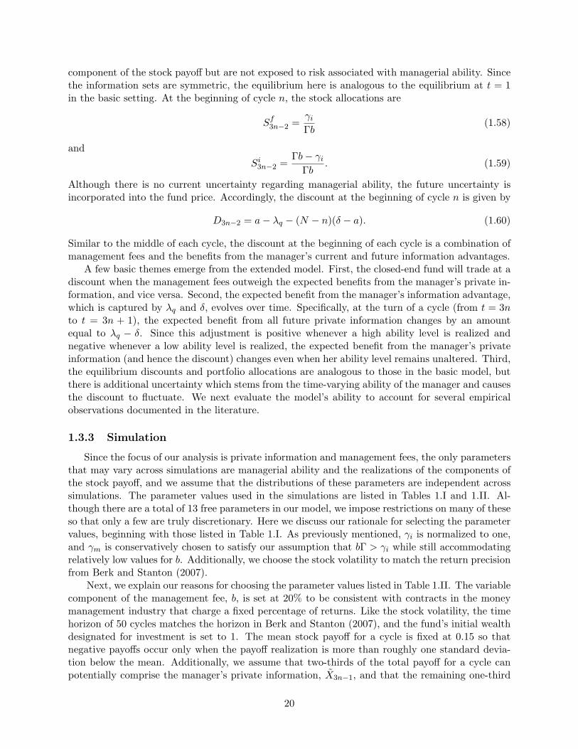
Since the focus of our analysis is private information and management fees, the only parametersthat may vary across simulations are managerial ability and the realizations of the components ofthe stock payoff, and we assume that the distributions of these parameters are independent acrosssimulations. The parameter values used in the simulations are listed in Tables 1.I and 1.II. Al-though there are a total of 13 free parameters in our model, we impose restrictions on many of theseso that only a few are truly discretionary. Here we discuss our rationale for selecting the parametervalues, beginning with those listed in Table 1.I. As previously mentioned, γi is normalized to one,and γm is conservatively chosen to satisfy our assumption that bΓ > γi while still accommodatingrelatively low values for b. Additionally, we choose the stock volatility to match the return precisionfrom Berk and Stanton (2007).

Next, we explain our reasons for choosing the parameter values listed in Table 1.II. The variablecomponent of the management fee, b, is set at 20% to be consistent with contracts in the moneymanagement industry that charge a fixed percentage of returns. Like the stock volatility, the timehorizon of 50 cycles matches the horizon in Berk and Stanton (2007), and the fund’s initial wealthdesignated for investment is set to 1. The mean stock payoff for a cycle is fixed at 0.15 so thatnegative payoffs occur only when the payoff realization is more than roughly one standard devia-tion below the mean. Additionally, we assume that two-thirds of the total payoff for a cycle canpotentially comprise the manager’s private information, X3n−1, and that the remaining one-third

20

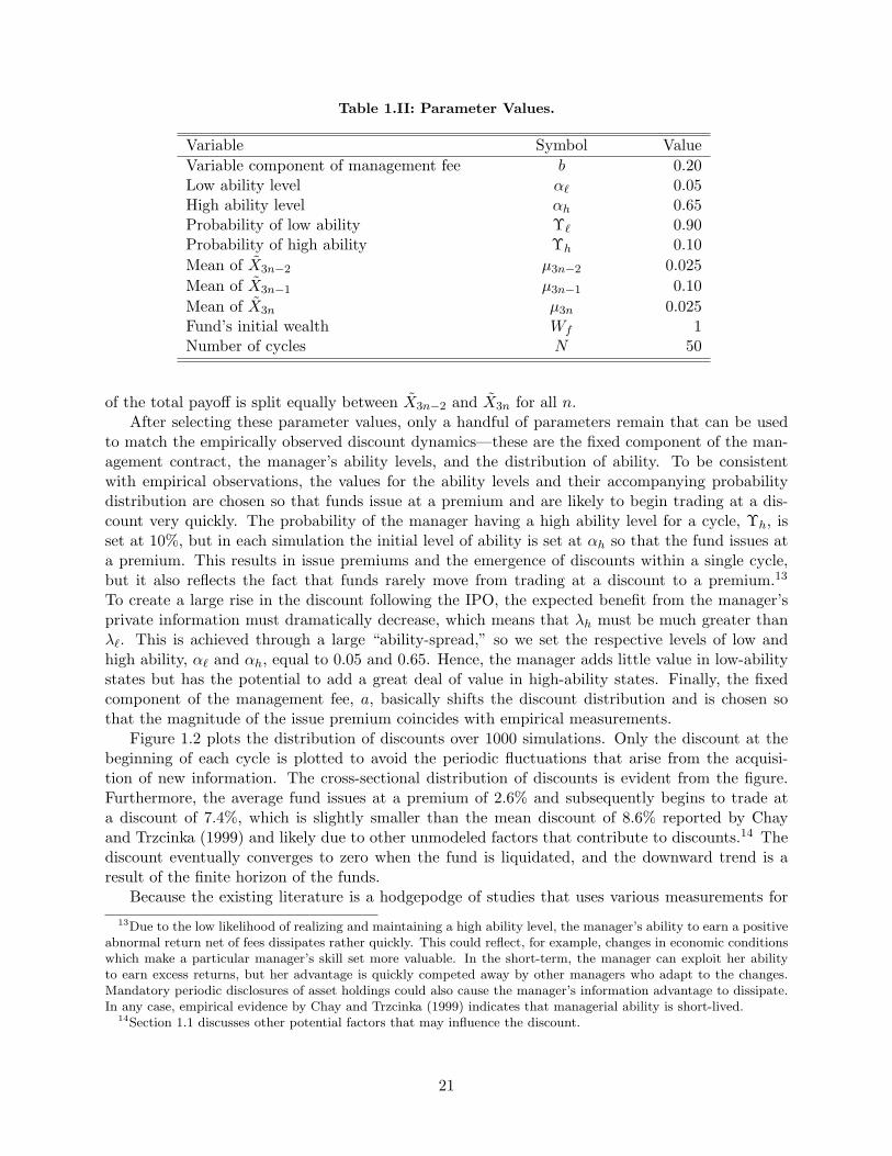
Table 1.II: Parameter Values.

Variable Symbol ValueVariable component of management fee b 0.20Low ability level α` 0.05High ability level αh 0.65Probability of low ability Υ` 0.90Probability of high ability Υh 0.10Mean of X3n−2 µ3n−2 0.025Mean of X3n−1 µ3n−1 0.10Mean of X3n µ3n 0.025Fund’s initial wealth Wf 1Number of cycles N 50

of the total payoff is split equally between X3n−2 and X3n for all n.After selecting these parameter values, only a handful of parameters remain that can be used

to match the empirically observed discount dynamics—these are the fixed component of the man-agement contract, the manager’s ability levels, and the distribution of ability. To be consistentwith empirical observations, the values for the ability levels and their accompanying probabilitydistribution are chosen so that funds issue at a premium and are likely to begin trading at a dis-count very quickly. The probability of the manager having a high ability level for a cycle, Υh, isset at 10%, but in each simulation the initial level of ability is set at αh so that the fund issues ata premium. This results in issue premiums and the emergence of discounts within a single cycle,but it also reflects the fact that funds rarely move from trading at a discount to a premium.13

To create a large rise in the discount following the IPO, the expected benefit from the manager’sprivate information must dramatically decrease, which means that λh must be much greater thanλ`. This is achieved through a large “ability-spread,” so we set the respective levels of low andhigh ability, α` and αh, equal to 0.05 and 0.65. Hence, the manager adds little value in low-abilitystates but has the potential to add a great deal of value in high-ability states. Finally, the fixedcomponent of the management fee, a, basically shifts the discount distribution and is chosen sothat the magnitude of the issue premium coincides with empirical measurements.

Figure 1.2 plots the distribution of discounts over 1000 simulations. Only the discount at thebeginning of each cycle is plotted to avoid the periodic fluctuations that arise from the acquisi-tion of new information. The cross-sectional distribution of discounts is evident from the figure.Furthermore, the average fund issues at a premium of 2.6% and subsequently begins to trade ata discount of 7.4%, which is slightly smaller than the mean discount of 8.6% reported by Chayand Trzcinka (1999) and likely due to other unmodeled factors that contribute to discounts.14 Thediscount eventually converges to zero when the fund is liquidated, and the downward trend is aresult of the finite horizon of the funds.

Because the existing literature is a hodgepodge of studies that uses various measurements for13Due to the low likelihood of realizing and maintaining a high ability level, the manager’s ability to earn a positive

abnormal return net of fees dissipates rather quickly. This could reflect, for example, changes in economic conditionswhich make a particular manager’s skill set more valuable. In the short-term, the manager can exploit her abilityto earn excess returns, but her advantage is quickly competed away by other managers who adapt to the changes.Mandatory periodic disclosures of asset holdings could also cause the manager’s information advantage to dissipate.In any case, empirical evidence by Chay and Trzcinka (1999) indicates that managerial ability is short-lived.

14Section 1.1 discusses other potential factors that may influence the discount.

21

0 10 20 30 40 50−0.09

−0.06

−0.03

0

0.03

0.06

0.09

0.12

Time

log(

Dt)

50%

5%

25%

75%

95%

Figure 1.2: Distribution of Closed-End Fund Discounts. The plot shows the log discount at thebeginning of each cycle, defined as log(V3n−2/P

f3n−2). The dashed line represents the average discount, and

the solid lines represent various fractiles of the discount distribution for 1000 simulated funds.

the discount—some use percentage discounts while others use log discounts or simple discounts15—in comparing the predictions of our model to existing empirical observations, we align our mea-surements with and attempt to replicate as close as possible the particular empirical study beingcompared. Additionally, the simulated data are modified prior to conducting our analyses. First,the data are smoothed, meaning that only observations from the beginning of each cycle are in-cluded. This reduces the effects of the synchronous information acquisition. Second, the first andlast observations are purged from each simulation, thereby eliminating the large and predictablerise (fall) in the discount that occurs during the first (last) cycle for almost every fund in thesimulated sample.

Relations Between Discounts and Returns

We first check whether the relations between discounts and returns in our model are compatiblewith empirical observations. As a preliminary matter, augmented Dickey-Fuller tests reject a unitroot at the 10% level for over 95% of the simulated funds, which indicates that the discounts arestationary. This result compares favorably to Pontiff (1995), where a unit root is rejected for only53% of funds in his sample.

Next, we evaluate the time-series correlations between log premiums, fund price returns, andNAV returns. To be consistent with Pontiff (1995), each individual pairwise correlation is weightedproportional to the inverse of the correlation’s standard error, and the weighted averages of thesecorrelations are presented in Table 1.III. The columns contain the contemporaneous variable, andthe rows contain the time-t variable.

The results from the simulation account for some prominent stylized facts found in the literatureand are for the most part qualitatively consistent with those reported by Pontiff (1995), althoughrigorous quantitative comparisons are difficult due to the mismatched frequency of the data. Someof the more puzzling statistical relations with which the model is consistent include: positively au-

15Percentage discounts are defined as one minus the ratio of the fund price to the fund’s NAV. Log discounts aredefined as the natural logarithm of the ratio of the fund’s NAV to the fund price. Simple discounts are defined asthe difference between the fund’s NAV and the fund price.

22

Table 1.III: Average Correlation Coefficients. A weighted average of the beginning-of-cycle individualpairwise correlation coefficients between premiums and returns over 1000 simulations is reported. Thecolumns contain the contemporaneous variables, and the rows contain the time-τ variables, where τ ≡ 3n−2is the beginning of the contemporaneous cycle, τ − 1 ≡ 3n − 5 is the beginning of the previous cycle, andτ + 1 ≡ 3n + 1 is the beginning of the next cycle. Premiums are defined as − log(Vτ/P fτ ), fund returnsare defined as log(P fτ+1/P

fτ ), and NAV returns are defined as log(Vτ+1/Vτ ). The weight of each individual

pairwise correlation coefficient is equal to the inverse of that correlation coefficient’s standard error.

Premiumτ Fund Returnτ NAV ReturnτPremiumτ−1 0.381

Fund Returnτ−1 0.416 −0.007Fund Returnτ 0.020Fund Returnτ+1 −0.064

NAV Returnτ−1 0.020 −0.025 −0.022NAV Returnτ 0.415 0.829NAV Returnτ+1 −0.055 0.243

tocorrelated premiums (discounts are persistent); a negative correlation between current premiumsand future fund returns (premiums predict fund returns); near zero correlation between currentpremiums and future NAV returns (premiums do not predict NAV returns); and less than perfectcontemporaneous correlation between fund returns and NAV returns (something besides NAV af-fects fund prices). Consistent with other empirically observed statistical relations, our model alsopredicts that current premiums are positively correlated with lagged fund returns but unrelated tolagged NAV returns and that current fund returns are unrelated to lagged NAV returns.

There are, however, a few discrepancies between the simulation results and empirical observa-tions. Pontiff (1995) finds that both fund returns and NAV returns are negatively autocorrelatedwhile our simulation produces autocorrelations near zero. He also reports a negative contempora-neous correlation between premiums and NAV returns and a negative correlation between currentfund returns and future NAV returns while our simulation yields positive correlations. Despitethese differences, the model performs relatively well in matching the time-series correlations be-tween discounts and returns reported in the literature.

Our model also accounts for some cross-sectional relations between discounts and returns. Theaverage correlation between changes in percentage discounts and the returns on the stocks held by afund in the simulation is −0.019, which is analogous to an observation by Lee, Shleifer, and Thaler(1991) that the correlation between changes in discounts and returns on a market index is aboutzero. Furthermore, our model produces an average correlation between changes in log premiumsand NAV returns of −0.334, which is consistent with a finding by Pontiff (1997) that the monthlycovariance between changes in log premiums and NAV returns is negative.

Based on the above comparisons, it appears as though the model adequately accounts for theempirically observed relations between discounts and returns. We next test whether fund returnsin our model are more volatile than NAV returns, as documented in the literature.

Excess Volatility of Fund Returns

Pontiff (1997) finds that fund returns are more volatile than the returns of their underlyingassets. He also reports a negative correlation between NAV returns and changes in premiums,which means that fund prices underreact to NAV returns. Together, these two observations are

23

perplexing because they indicate that fund prices are more volatile than NAV returns even thoughprices tend to underreact to NAV returns. In the previous subsection, we report that our modelleads to a negative correlation between changes in premiums and NAV returns. In this subsection,we assess whether our model produces fund returns that are more volatile than the underlying NAVreturns. We find that it does.

For each fund in the sample, the log of the ratio of the fund return variance to the fund’sNAV return variance is calculated. A positive log variance ratio indicates that the volatility of thefund return is greater than the volatility of the underlying NAV return. The average log varianceratio from the simulations is approximately 0.122 and is significantly different from zero, althoughit is smaller than the four-month average log variance ratio of 0.434 reported by Pontiff (1997).Nevertheless, our model accounts for the excess volatility of fund returns.

The primary source of excess volatility is the discount itself, which is best appreciated byconsidering the NAV return over a single cycle, Rv ≡ V3n+1/V3n−2, and the fund return over asingle cycle, Rf ≡ P f3n+1/P

f3n−2. Given V3n−2, the conditional variance of the NAV return is

V[Rv |V3n−2

]=

V[V3n+1]V 2

3n−2

, (1.61)

where V is the variance operator, and the conditional variance of the fund return can be written as

V[Rf |P3n−2, V3n−2

]=

V[V3n+1] + V[λ](V3n−2 −D3n−2)2

(1.62)

after substituting (1.60) since the NAV return for the current cycle is independent of the manager’sability during the ensuing cycle. Comparing these expressions, it is evident that if the fund istrading at a discount (i.e., D3n−2 > 0) then the variance of the fund return is greater than thevariance of the NAV return. On the other hand, if the fund is trading at a premium then thevariance of the fund return may or may not be greater than the variance of the NAV return,depending on the size of the premium and the variance of λ. Furthermore, our conclusion that thediscount is the primary source of a fund’s excess volatility is consistent with a finding by Pontiff(1997) that the excess volatility is unrelated to market factors since discounts in our model dependon the ability of the manager.

Profitable Trading Strategies

Perhaps one of the most anomalous empirical observations is that closed-end funds with largediscounts tend to outperform the market while those with large premiums tend to underperformthe market, adjusted for risk, as documented by Thompson (1978) and Pontiff (1995). Given ourcurrent set of assumptions, our model is unable to account for such underperformance. By slightlymodifying our assumptions, however, our model not only produces underperforming premium fundsbut also provides an economic explanation for this phenomenon. Specifically, our model producesunderperforming premium funds when the stock price is endogenously determined. We formallydescribe the modifications to our model that will generate underperformance of premium funds inAppendix A.1, though we note here that endogenizing the stock price does not alter either the fun-damental concept of our model or the nature of our analysis. Indeed, the only practical differencebetween the equilibrium in our featured model described in Section 1.3.2 and in our modified modelis the extent to which the manager can profit from her information advantage, as an endogenousstock price influences how aggressively the manager trades on her private information. In this sub-section, we first demonstrate the aforementioned underperformance using simulated data from our

24

Table 1.IV: Risk-Adjusted Performance. The returns from an equally-weighted dynamic portfolio thatis long the 2% of funds with the largest discount are regressed on the returns from an equally-weightedportfolio of the stocks traded by the those funds and the returns from an equally-weighted dynamic portfoliothat is short the 2% of funds with the largest premium are regressed on the returns from an equally-weightedportfolio of the stocks traded by those funds. The returns from an equally-weighted portfolio of all funds areregressed on the returns from a portfolio of all stocks. The coefficients from these regressions are presentedwith t-statistics in parentheses. Significance at the 95% level is indicated by ∗∗, and significance at the 99%level is indicated by ∗∗∗.

Discount Premium All Funds

Jensen’s alpha−0.083 3.714 −0.003(−0.46) (3.73)∗∗∗ (−0.01)

Beta with stock index0.756 −2.269 0.416

(4.17)∗∗∗ (−2.28)∗∗ (1.48)

modified model with an endogenous stock price. We then explain why significant underperformancedoes not occur under our original set of assumptions with an exogenous price process.

To assess whether our model generates premium (discount) funds that underperform (outper-form) the market, we analyze two distinct investment strategies as in Pontiff (1995). The firststrategy entails forming an equally-weighted dynamic portfolio, which we refer to as the “discountportfolio,” consisting of the 2% of funds that have the largest discount. The second strategy involvesthe construction of another equally-weighted dynamic portfolio, which we refer to as the “premiumportfolio,” consisting of the 2% of funds that have the largest premium.16 These portfolios areinitially created at the beginning of the second cycle and are held until the beginning of the nextcycle, at which point they are rebalanced. The process repeats for N − 2 cycles.

The returns from holding a long position in the discount portfolio and a short position in thepremium portfolio are regressed on the returns from an equally-weighted portfolio comprised ofthe stocks traded by the funds in the respective portfolios. As a benchmark, the returns froman equally-weighted portfolio comprising all simulated funds are regressed on the returns from anequally-weighted portfolio of all simulated stocks. The coefficients from these regressions are re-ported in Table 1.IV. There is a positive and highly significant risk-adjusted abnormal return forthe shorted premium portfolio, measured as the intercept from the aforementioned regressions asin Jensen (1968). The risk-adjusted abnormal returns for the discount portfolio and the benchmarkportfolio are not significantly different from zero. Thus, it appears as though funds in our modelthat trade at a premium significantly underperform the market, adjusted for risk, but funds thattrade at a discount do not outperform the market on a risk-adjusted basis.

To illustrate the extent of the profits that can be earned by buying funds that trade at a largediscount and selling funds that trade at a large premium, we calculate the returns accruing to boththe discount portfolio and the premium portfolio. Table 1.V reports the terminal value of one dollarinvested at the beginning of the second cycle for each of these strategies, along with an equally-weighted benchmark portfolio comprising all simulated funds. The discount portfolio outperformsthe benchmark portfolio by 16%, while the premium portfolio underperforms the benchmark port-folio by 55% over N − 2 cycles.

Given the documented poor relative performance of closed-end funds that trade at a premium,the question remains: why do investors purchase closed-end funds that trade at a premium? Theanswer, we argue, is that large-premium funds provide insurance against extreme realizations of

16The results presented below are robust to portfolios of various sizes within the neighborhood of 2%.

25

Table 1.V: Illustration of Returns. One dollar is invested in an equally-weighted dynamic portfolioconsisting of the 2% of funds with the largest discount and an equally-weighted dynamic portfolio consistingof the 2% of funds with the largest premium. Each portfolio is rebalanced at the beginning of every cycle. Aportfolio comprising all funds serves as a benchmark. The terminal value is the return from the investmentover N − 2 cycles. The intra-cycle return is the return accruing within cycles, and the inter-cycle return isthe return accruing between cycles. The average excess return is the time-series average of the differencebetween either the discount portfolio or the premium portfolio and the benchmark portfolio. t-statistics arein parentheses. Significance at the 95% and 99% levels are indicated by ∗∗ and ∗∗∗, respectively.

Discount Premium All FundsTerminal value 1.126 0.442 0.974

Intra-cycle return 1.086 0.436 1.011Inter-cycle return 1.037 1.012 0.963

Average excess return0.309 −1.568

(2.00)∗∗ (−3.06)∗∗∗

the manager’s private information. A fund will trade at a premium in our model only when themanager has a high level of ability, which allows her to observe a larger portion of the stock payoff.The high ability level, however, does not necessarily translate into positive abnormal returns netof management fees. If the realization of Zn,1 is close to αqµ3n−1, then the manager’s private infor-mation is less valuable in the sense that knowledge of Zn,1 does not dramatically alter the fund’sportfolio composition. On the other hand, the private information is tremendously valuable givenan extreme realization of Zn,1. If Zn,1 is very small, then the fund will hold less stock and therebyavoid a hefty loss that otherwise would have been incurred; alternatively, if Zn,1 is really large, thenthe fund will hold more stock and thereby earn a sizable gain that otherwise would not have beenrealized. Because the investor is risk-averse, he is willing to purchase shares in the fund to obtainthe abnormal return when the stock payoff is low even though he expects the fund to underperformon average. Conversely, there is no insurance component of a fund that trades at a large discountsince the manager of such a fund has low ability. As is evident from Figure 1.3, which plots thenet-of-fee returns of premium and discount funds as a function of Zn,1, the single-cycle returns forfunds that trade at a premium tend to be quite large for extreme realizations of Zn,1 but negativefor non-extreme realizations, while the returns for funds that trade at a discount tend to clusteraround zero.

The concept of insurance in the portfolio delegation setting is not unique to closed-end funds.For instance, Glode (2011) demonstrates that insurance concerns drive the negative risk-adjustedperformance of open-end mutual funds. In his model, fund managers actively seek abnormal returnsin bad states of the economy, and these active returns covary positively with the pricing kernel. Inour model, however, insurance does not necessarily imply a positive relation between the pricingkernel and abnormal returns of funds that trade at a premium since abnormal returns are alsoearned in extremely good states.

A closer inspection of the returns accruing to the discount and premium portfolios from theabove illustration provides some evidence in favor of the insurance argument. The aggregate returnof each portfolio can be decomposed into the return accruing within cycles (from t = 3n− 2 to 3n)and the return accruing between cycles (from t = 3n to 3n+ 1), and Table 1.V lists the intra-cycleand inter-cycle returns of both the discount portfolio and the premium portfolio. A fair portionof the returns accruing to the discount portfolio occurs between cycles. This suggests that highability shocks, which possibly could be attributed to manager replacement as in Wermers, Wu, andZechner (2008), contribute to the excess return for the discount portfolio. Conversely, the premium

26

−0.2 −0.1 0 0.1 0.2 0.3 0.4−0.4

−0.2

0

0.2

0.4

0.6

Zτ

Fun

d R

etur

n τ

(a) Premium Fund Returns

−0.2 −0.1 0 0.1 0.2 0.3 0.4−0.4

−0.2

0

0.2

0.4

0.6

Zτ

Fun

d R

etur

n τ

(b) Discount Fund Returns

Figure 1.3: Fund Returns. The plots show the log fund returns over a cycle, defined as log(P f3n+1/Pf3n−2),

as a function of the realization of Zn,1. Panel (a) plots the returns for funds that are trading at a premiumat the beginning of the cycle, and panel (b) plots the returns for funds that are trading at a discount at thebeginning of the cycle.

portfolio losses are amassed within cycles, suggesting that ability shocks play a minimal role inthe returns of funds that trade at a premium. Since a premium fund earns negative returns netof management fees when there are non-extreme realizations of Zn,1, the losses accruing to thepremium portfolio are a result of the insurance against extreme realizations of Zn,1 failing to pay.

While premium funds in our model tend to underperform when the stock price is endogenouslydetermined, no such underperformance occurs when the stock price follows an exogenous process.This is due to the fact that the stock price influences how aggressively the manager trades on herprivate information, but the price does not respond to the manager’s trades when it follows anexogenous process. As a result, the manager can better exploit her information advantage whenthe stock price is exogenous. At the times when the manager possesses an information advantageover the investor, her stock allocations with an exogenous (from (1.55)) and endogenous (from(A.2) Appendix A.1) price can be rewritten as

Sf3n−1 =1

(1− αq)γmbσ23n−1

[(Zn,1 − αqµ3n−1

)+γiγm

Γσ2

3n−1

](1.63)

andSf3n−1 =

Γb− γiγmb

(αqγi + (1− αq)Γb

)σ2

3n−1

[(Zn,1 − αqµ3n−1

)+

γiγmb

Γb− γiσ2

3n−1

], (1.64)

respectively. The first term inside the brackets in each of these equations represents the aggressive-ness with which the manager trades on her information advantage while the second term capturesthe portfolio adjustment resulting from a reduction in risk (since the manager observes a portion ofX3n−1) that is independent of the specific realization of the manager’s private information. Com-paring the coefficients on these two equations reveals that the manager trades more aggressivelywhen the stock price is exogenous. Consequently, she can better capitalize on her informationadvantage to earn much larger abnormal returns with an exogenous stock price, which means thatpremium funds in our model do not underperform when the stock price is exogenous.

27

1.4 Conclusion

We present a dynamic partial equilibrium model in which a closed-end fund manager periodicallyacquires private information about the future performance of an underlying asset. Although themanager adds value by exploiting her information, whether the fund trades at a premium or discountdepends on the value of her private information in relation to the management fees. Our modelaccounts for several empirically observed characteristics of closed-end funds. Funds in our modelissue at a premium but rapidly move into a discount, and there is both cross-sectional and time-series variation in discounts. The model also is consistent with the observed relations betweendiscounts and returns, as well as the excess volatility of fund returns. The model explains whyfunds issue at a premium and provides a justification as to why investors purchase seasoned fundsthat trade at a premium even though they are expected to underperform funds that trade at alarge discount.

28

Chapter 2

Activist Arbitrage, Lifeboats, andClosed-End Funds

We present a dynamic rational expectations model of closed-end fund discounts that incorpo-rates feedback effects from activist arbitrage and lifeboat provisions. We find that the potentialfor activism and the existence of a lifeboat both lead to narrower discounts. Furthermore, bothactivist arbitrage and lifeboats effectuate an ex post transfer of wealth from managers to investorsbut an ex ante transfer of wealth from low-ability managers to high-ability managers. On average,investor wealth is unaffected by either activist arbitrage or lifeboats because their potential benefitsare factored into higher fund prices. Although lifeboats can reduce takeover attempts, they do notincrease expected managerial wealth.

2.1 Introduction

Closed-end funds are investment companies that hold a portfolio of financial assets, but unlikemutual funds, closed-end funds issue a fixed number of non-redeemable shares that trade at pricesdetermined by the market. Most funds tend to trade at a discount relative to their net asset value(NAV), which means that a profit can be earned by terminating the fund and distributing its as-sets to the shareholders, as demonstrated by Brickley and Schallheim (1985). This potential for aquick profit creates an incentive for an outsider to purchase shares in a discounted fund and forcea liquidation—a process known as activist arbitrage.

Activist arbitrage involves purchasing shares in a fund that is trading at a discount, taking someaction in an attempt to eliminate the discount, and subsequently redeeming the shares at NAV ifthe endeavor is successful. Although accurately predicting which funds an activist arbitrageur willtarget is extremely difficult, Bradley, Brav, Goldstein, and Jiang (2010) find that activists tendto seek out funds that trade at large discounts, likely because there are greater financial returnsto be realized when these funds restructure. Since ordinary investors share in the profit createdby an activist, rational investors will recognize that a fund with a deep discount may become thetarget of an activist and purchase shares in the fund, hoping to piggy-back on the activist’s efforts.In doing so, they will bid up the fund price, thereby causing the discount to shrink. This makesthe closed-end fund a less attractive target and activist arbitrage less likely to occur. Thus, thepotential for activist arbitrage creates an interesting “feedback loop” whereby, in equilibrium, thediscount accurately reflects investors’ beliefs regarding the probability of activism.

Lifeboats are another source of feedback on closed-end fund prices. A lifeboat is a provision,usually contained in a fund’s prospectus, that describes remedial actions for the fund to undertake

29

to reduce or eliminate the discount if the fund price drops below a predetermined level. Commonlifeboats include implementing a managed distribution plan (MDP), conducting a tender offer atNAV, repurchasing shares at market price, or converting to an open-end mutual fund. For reasonsoutlined below, we focus solely on MDPs, which mandate minimum periodic dividend distributionsto a fund’s shareholders. Regardless of the specific type of lifeboat, the potential beneficial effectsof a lifeboat will result in higher prices, thereby making it less likely that the lifeboat will be trig-gered. Like with the potential for activist arbitrage, the equilibrium discount must incorporate thisfeedback effect in a way that accurately reflects investors’ expectations about the future impact ofthe lifeboat.

Due to the aforementioned feedback loops, the interaction between closed-end fund prices, ac-tivist arbitrage, and lifeboat provisions is nontrivial. To better understand the equilibrium relation-ships between activist arbitrage, lifeboats, and closed-end funds, we construct a dynamic rationalexpectations equilibrium model of closed-end fund discounts that incorporates the feedback effectsfrom these two important institutional features.1 Our model is a discrete-time extension of themodel presented by Berk and Stanton (2007) but differs from theirs by allowing for the endoge-nous triggering of a lifeboat provision and initiation of a restructuring attempt. In our model, thedivergence between NAV and the fund price arises from a tradeoff between management fees and amanager’s ability to generate excess returns. As the discount grows, the probability of an activistinitiating a restructuring attempt increases, as does the probability of triggering the lifeboat. Atthe same time, the presence of activist arbitrageurs and lifeboat provisions exerts upward pressureon the fund price, causing the discount to shrink. Our model also incorporates the fact that fundgovernance characteristics, such as supermajority voting requirements (Bradley, Brav, Goldstein,and Jiang (2010)) or the existence of staggered boards (Del Guercio, Dann, and Partch (2003)),affect the incidence of activism as well as the fact that different lifeboat parameters, such as thedividend payout rate and lifeboat trigger level, influence the impact of lifeboats on closed-end funds.

We obtain analytical expressions for the discount in a variety of settings: where no activist orlifeboat exists, where only an activist exists, where only a lifeboat exists, and where both an ac-tivist and a lifeboat exist. Our solutions are not in closed-form, however, so we conduct a numericalsimulation to ascertain the impact of activist arbitrage and lifeboats on closed-end funds. In theabsence of both activist arbitrageurs and lifeboats, a discount emerges whenever investors believethat management fees outweigh the manager’s contribution. Using this setting as a benchmark, wediscover that activist arbitrage and lifeboat provisions influence funds in a number of ways.

Both activism and lifeboats independently cause fund prices to rise, which results in funds is-suing at a larger premium than when neither an activist nor a lifeboat is present. The magnitudeand persistence of the increased prices depends on the ability of the fund manager, with a greatereffect on funds with low-ability managers. The primary function of activism and lifeboats, however,is to provide insurance against poor management. When prompted, both activist arbitrage andlifeboat provisions effectuate an ex post transfer of wealth from managers to investors, but sincefunds with high-quality management are less likely to have their lifeboats triggered or encounteran activist arbitrageur, the increased issue premium results in an ex ante expected wealth transferfrom low-ability managers to high-ability managers. On average, investors neither gain nor losefrom either activist arbitrage or lifeboat provisions because their potential benefits are incorporatedinto higher fund prices.

Consistent with empirical observations by Brauer (1984) and Brickley and Schallheim (1985),funds in our model that are successfully liquidated tend to have deeper discounts prior to the liq-

1In contrast to previous studies by Lee, Shleifer, and Thaler (1991), Berk and Stanton (2007), Cherkes, Sagi, andStanton (2009), Lenkey (2011), and others, we do not attempt to explain the source of closed-end fund discounts.See, e.g., Dimson and Minio-Kozerski (1999) for a survey of the closed-end fund literature.

30

uidation event than funds that are not liquidated, and large abnormal returns occur at the timeof a liquidation announcement. Additionally, funds in our model with an MDP have narrower dis-counts than funds without an MDP, and discounts shrink upon the adoption of an MDP, which isconsistent with empirical findings by Johnson, Lin, and Song (2006) and Wang and Nanda (2008).

When activist arbitrageurs and lifeboat provisions coexist, MDPs tend to be adopted less fre-quently and fewer reorganizations take place. We find that introducing a lifeboat has the greatestimpact when activist arbitrage is unlikely to occur and that activist arbitrage has the biggest effectwhen the lifeboat is unlikely to be triggered. In other words, activism and lifeboats serve as sub-stitutes for one another. Furthermore, introducing a lifeboat to an environment where an activistarbitrageur already exists provides additional insurance against low-ability management only whenthe lifeboat is liable to be triggered.

Since fund managers face a loss of wealth and non-pecuniary benefits when a restructuringoccurs, as demonstrated by Brauer (1984), some authors have suggested that a lifeboat can be usedto ward off activist arbitrageurs by mitigating a fund’s discount.2 While lifeboats do indeed lessenthe severity of discounts and decrease the incidence of restructuring events, our results indicatethat lifeboats are not a suitable means for enhancing managerial wealth. On the contrary, we findthat an MDP decreases the expected value of management fees over the life of a fund, even whenthe fund might potentially face a premature liquidation caused by an activist arbitrageur. This isbecause an MDP itself facilitates a partial liquidation of the fund.

Despite an extensive amount of academic research on closed-end funds, there is a paucity of the-oretical models in the closed-end fund literature that include either activist arbitrage or lifeboats.To the best of our knowledge, our work is the first truly dynamic model of fund discounts that in-corporates activist arbitrage and lifeboat provisions. In a static setting, Deaves and Krinsky (1994)model a tradeoff between managerial ability and fees, with an exogenous probability of open-endingthat depends on the difference between ability and fees. They demonstrate numerically that therelationship between the discount and probability of restructuring is not monotonic, but that ahigher probability of restructuring leads to a narrower discount over a range of values. Cherkes,Sagi, and Wang (2009) model a sequential game between a fund manager and activist wherein thefund manager can implement an MDP with the purpose of reducing the financial incentive for anactivist to attempt a restructuring. Empirically, they find that funds with an MDP experiencefewer attacks and are less likely to be liquidated than funds without an MDP. Their model, how-ever, does not account for the time-series dynamics of closed-end funds.

Our current work also contributes to the growing literature on feedback loops in more general fi-nancial market settings. Edmans, Goldstein, and Jiang (2012) study the interaction between marketprices and takeover attempts of industrial firms. Empirically, they find that investors anticipatingtakeovers drive up prices, thereby deterring takeover activity. Bond, Goldstein, and Prescott (2010)investigate the equilibrium implications where a market activist does not observe fundamentals butdecides whether to intervene based on prices. In contrast to their model, prices in our model affectthe likelihood of activism but do not influence the activist’s beliefs about fundamentals (managerialability). Moreover, our analysis focuses on how different fund governance characteristics as well asvarious parameterizations of a lifeboat provision affect equilibrium discounts, returns, and expectedwealth.

The remainder of the paper is organized as follows. In Section 2.2, we derive analytical ex-pressions for the discount in a variety of settings. We then present the results from a simulationanalysis in Section 2.3. Finally, Section 2.4 concludes.

2See, e.g., Cherkes, Sagi, and Wang (2009) and Johnson, Lin, and Song (2006).

31

2.2 Model

The general framework of our benchmark model, which does not include either activist arbitrageor lifeboats, is a discrete-time analog of Berk and Stanton (2007). We later incorporate activismand lifeboats in Sections 2.2.2 and 2.2.3, respectively. In our benchmark model, closed-end funddiscounts result from a tradeoff between management fees and a fund manager’s perceived abilityto generate excess returns. Rational investors form beliefs about managerial ability and updatethem over time based on observed fund returns. Accordingly, funds trade at a discount when-ever investors believe that management fees outweigh the expected value created by the manager’sability, and vice versa. The key insight of Berk and Stanton (2007), which we also incorporateinto our model, is that the fund manager’s compensation can never fall but will increase wheneverhis perceived ability rises above a certain level. This compensation structure reflects the optimalmanagerial contract derived by Harris and Holmstrom (1982) (where wages are never decreasedbut employees receive pay raises) extended to a labor market with frictions, such as costly jobswitching. The specific (unmodeled) form of the manager’s pay raise is assumed to be an influx ofcapital to manage through a rights offering or the creation of a new fund, which reduces his abilityto generate excess returns since his fixed skill level is spread thinner over the additional capitalunder management. This mechanism is also employed by Berk and Green (2004) to explain theflow of capital in mutual funds.

Although conceptually identical to Berk and Stanton (2007), our benchmark model is mathemat-ically very different from theirs. While they model an economy in continuous time with normallydistributed excess returns and normally distributed managerial ability, we find it more naturalto model activism and lifeboat events in discrete time due to the existing institutional practicessurrounding reorganizations and lifeboats, as both reorganizations and lifeboat implementations fre-quently require shareholder approval, which often comes from proxy votes at a shareholder meetingthat may not occur until months after a lifeboat is triggered or an attack is initiated by activist.Furthermore, since activist arbitrage and lifeboat provisions can give rise to truncated distribu-tions of otherwise normally distributed future fund discounts, we assume that excess returns areBernoulli distributed to lessen the computational burden. We also find it computationally con-venient to assume a uniform distribution for managerial ability when we conduct our simulationanalysis in Section 2.3. These different assumptions necessitate the construction of a model that isdistinct from Berk and Stanton (2007), even though the broad concepts are the same.

We explicitly model only a single asset—a closed-end fund. Trading in the financial marketoccurs at discrete dates indexed by t = 1, 2, . . . , T . The closed-end fund undergoes an initial publicoffering (IPO) at t = 1 and is scheduled to liquidate at T , at which time the fund’s shareholdersreceive the value of the assets under management.

The closed-end fund earns a gross return during each period that is comprised of two com-ponents. The first component is a random return from a portfolio of financial assets held by thefund. Let rt+1 denote the return on the fund’s portfolio from time t to t+ 1. This return is seriallyindependent and observable by all parties. The second component of the fund’s gross return is arandom excess return generated by a fund manager. The excess return, which is also observableby all parties, from time t to t + 1 is given by the product γtαt+1, where αt+1 ∈ {α`, αh} andγt ∈ [0, 1]. Here, αt+1 denotes the potential excess return that can be generated during a period,but as discussed in more detail below, this potential excess return is scaled by γt. Additionally,αt+1 is uncorrelated with the return on the fund’s portfolio both contemporaneously and acrosstime. To compensate the manager, a management fee, φ, that is equal to a fixed percentage of theassets under management is assessed on the fund each period.

The true probability that the manager earns a high excess return, αh, during a period is denoted

32

by Π and is constant over time. Accordingly, a low excess return, α`, will be realized with probabil-ity 1− Π. This probability is exogenous and unobservable, but investors form beliefs regarding Πwhich evolve over time in a Bayesian fashion. Let πt denote the investors’ beliefs about Π at timet. The posterior probability of πt, conditional on observing n high excess returns after t periods,follows a beta distribution with parameters at and bt: πt ∼ Beta (at, bt). If the prior parametersare a1 and b1 so that π1 ∼ Beta (a1, b1), then it follows immediately from DeGroot (2004, p. 160,Theorem 1) that the posterior parameters are at = a1 + n and bt = b1 + t− n. Furthermore, sinceαt+1 is Bernoulli distributed, the marginal distribution of αt+1 is a beta-binomial distribution butreduces to a Bernoulli distribution. Therefore, investors rationally believe that a high excess returnwill occur with posterior probability given by

πt =at

at + bt,

which evolves according to

πt+1 = πt +χt+1 (at + bt)− at

(at + bt) (at + bt + 1), (2.1)

where χt+1 is an indicator function that takes the value one if αt+1 = αh and zero otherwise.As in Berk and Stanton (2007), we assume that the fund manager is compensated using an

insurance contract, pursuant to which the manager’s wage may never fall but may increase wheneverthe manager’s perceived ability,

α∗t ≡ γt [πtαh + (1− πt)α`] ,

rises above a particular exogenous threshold, Υ.3 Specifically, we assume that if α∗t would otherwisebe greater than Υ, then γt is adjusted downward to the point where the perceived ability at time tequals Υ. For all future dates, γt retains its newly-adjusted value unless the investors’ updated be-liefs would necessitate an additional downward adjustment. This mechanism reflects the manager’scapability to raise additional capital when his perceived ability to generate excess returns is high,which in turn reduces his ability to produce excess returns. Because the investors’ beliefs regardingΠ are unaffected by the adjustment process, the evolution of πt is still described by (2.1).

Assets in our model are priced as though investors are risk neutral. Consequently, the equilib-rium expected rate of return for all financial assets, including both the closed-end fund and theportfolio held by the fund, must equal the market expected rate of return, which is denoted by µ.Additionally, Pt denotes the fund price, Vt denotes the NAV of the fund, and

Dt ≡PtVt

(2.2)

denotes the fund discount at time t. A discount greater than one means that the fund trades at apremium.

We now proceed to derive analytical expressions for the closed-end fund discount in varioussettings. We first derive an expression for the discount in the absence of both an activist arbitrageur

3We assume that Υ is constant and independent of the existence of activist arbitrageurs or lifeboat provisions.Consequently, the evolution of γt is unaffected by the presence of either activists or lifeboats. Since managerialpay raises lead to larger discounts, ceteris paribus, it is plausible that managers could attempt to ward off activistsor decrease the likelihood of triggering a lifeboat by foregoing pay raises until the expected benefit from a raisingadditional capital outweighs the costs associated with an increased probability of an activist attack or a lifeboattrigger. In terms of our model, this would entail increasing the excess return adjustment threshold, Υ, which is liableto lead to less severe discounts. Therefore, our simulation results presented in Section 2.3 likely underestimate theimpact of activist arbitrage and lifeboats on closed-end fund discounts.

33

and a lifeboat provision in Section 2.2.1 to provide a benchmark for additional analysis. We theninvestigate the impact of activist arbitrage in Section 2.2.2 and the effect of a lifeboat provision inSection 2.2.3. Finally, we derive an expression for the discount in an environment with both anactivist arbitrageur and a lifeboat in Section 2.2.4.

2.2.1 Benchmark Discount

In the absence of both an activist arbitrageur and a lifeboat provision, the fund’s NAV returnis a combination of the return on the fund’s portfolio, the excess return generated by the manager,and the management fee. Therefore, NAV evolves as

Vt+1 = Vt (1 + rt+1 − φ+ γtαt+1) , (2.3)

and the expected one-period NAV return is

Et

[Rvt+1

]= M + γtEt [αt+1] , (2.4)

whereM ≡ 1 + µ− φ.

It is apparent from (2.4) that the expected NAV return generally will not equal the market expectedrate of return, µ. As a result, for the market to clear the fund price must adjust so that the expectedfund return,

Et

[Rft+1

]≡Et

[Pt+1

]Pt

, (2.5)

equals the market expected rate of return. Typically, the fund price will not equal NAV. Instead,the closed-end fund will trade at a discount described by the following proposition.4

Proposition 1. In the absence of both an activist arbitrageur and a lifeboat provision, the closed-end fund discount at each date t < T is

Dt =1

1 + µEt

[Dt+1 (M + γtαt+1)

]. (2.6)

While this proposition describes the discount for all dates t < T , the principle of no arbitrageimplies that at time T the discount vanishes, i.e., DT = 1.5 Additionally, the primary determinantof the discount is the relation between the management fee and the excess return generated bythe manager. A fund that generates zero expected excess return for all dates and charges no feesalways trades at NAV.

2.2.2 Activist Arbitrage

The goal of an activist arbitrageur is to eliminate the discount through a reorganization. Whilediscounts can be eliminated in a variety of ways—for instance, by converting the closed-end fundto an open-end mutual fund or by merging with an existing mutual fund—we focus solely on fundliquidation because it allows us to compute the impact of activism but avoids unnecessary compli-cations that might arise if the fund were to continue operating in a different form. Furthermore,

4Proofs for all Propositions are contained in Appendix B.2.5No arbitrage also implies that the discount at time T equals one in the other versions of the model discussed in

Sections 2.2.2, 2.2.3, and 2.2.4.

34

we make no assumptions regarding the specific mechanisms through which a restructuring attemptoccurs, although in reality activists tend to rely on proxy contests and non-binding shareholder pro-posals. As we demonstrate numerically in Section 2.3, activist arbitrage has the potential to impactclosed-end fund discounts through actual liquidation, unsuccessful liquidation attempts, and thepossibility of future liquidation attempts, even if the fund is never actually liquidated or attackedby an activist. In this section, we outline our assumptions and derive analytical expressions for thediscount in the presence of an activist arbitrageur.

Liquidating a fund via shareholder activism can take a substantial amount of time, possiblyentailing several rounds of shareholder proposals and proxy votes in the face of managerial resis-tance.6 While there is no guarantee that a liquidation attempt will be successful, the likelihoodof successfully liquidating a closed-end fund through activism depends, to a large extent, on thefund’s governance characteristics. Del Guercio, Dann, and Partch (2003) report that out of 42 fundrestructuring proposals over a 4 year period, the board of directors recommended against approvalin all 17 proposals that failed and in favor of approval in almost all 25 successful reorganizations.In a separate study, Brauer (1988) finds that managerial entrenchment can also hinder activism.Apparently, a fund’s board and management both strongly influence the success of a liquidationattempt. In our model, we assume that, given a liquidation attempt, the fund will successfully liq-uidate with probability q, which is exogenous and constant over time. Although we do not explicitlymodel the source of the liquidation probability, q could represent, inter alia, supermajority votingrequirements, the existence of staggered boards, the presence of large blockholders, or the ease ofcommunication between an activist and shareholders. Empirical evidence that these features affectthe probability of a successful restructuring is provided by Barclay, Holderness, and Pontiff (1993),Del Guercio, Dann, and Partch (2003), and Bradley et al. (2010).

If at time t− 1 an activist takes steps to initiate a liquidation attempt, the fund is consideredto be under attack at t, and the uncertainty regarding whether the undertaking will be successfulis resolved during the ensuing period. This could occur through, for example, a proxy vote oradoption of a shareholder proposal. If the liquidation attempt is successful, the closed-end fundwill liquidate at t+ 1. In such a case, the fund’s expected liquidation value is

Vt (M + γtEt [αt+1]) . (2.7)

If, on the other hand, the liquidation attempt fails, the fund retains its closed-end form with NAVevolving according to (2.3), but additional attempts may be made in the future. Because there isa two-period lag between the initiation of an attempt and the liquidation event, no attacks willcommence later than T − 3.7

For attempting a liquidation, an activist incurs a cost, c ∈ (0, 1), that is equal to a constantpercentage of NAV. We do not model the source of this cost, but it could comprise the costs ofactivism outlined by Grossman and Hart (1980), i.e., the cost of acquiring information about thetarget fund and administrative expenses associated with soliciting shareholders to approve the liq-uidation as well as with liquidating the fund if the attempt succeeds. Since an activist will notinitiate a liquidation attempt unless the expected gains from doing so outweigh the costs, we as-sume that no attempts will occur unless the discount falls below a certain threshold, κ (c, q), whichis a continuous function κ : (0, 1) × (0, 1) → [0, 1] that is decreasing in the cost of activism and

6See Bradley et al. (2010) for a detailed account of a restructuring attempt and Barclay, Holderness, and Pontiff(1993) or Del Guercio, Dann, and Partch (2003) for techniques that a large blockholder or board of directors mayutilize to defeat restructuring attempts.

7Barclay, Holderness, and Pontiff (1993) find that fund restructuring attempts are usually either successfullycompleted or abandoned within two years, and Brav et al. (2008) report that the median holding period for activisthedge funds that target industrial corporations is about 1.5 years.

35

increasing in the probability of liquidation. This attack threshold reflects the need for a largerprofit margin when costs are high or the likelihood of successful liquidation is low.

While the existence of a discount lower than the attack threshold is a necessary condition foractivism, it is not by itself sufficient. Empirically, not every fund that trades at a deep discountbecomes a target. Perhaps this is due to some idiosyncratic features of funds which we do not ex-plicitly model, such as managerial entrenchment, in combination with the small number of activistswho target closed-end funds.8 We incorporate this uncertainty of activism by assuming that theoccurrence of an attempt is random, with a deeper discount giving rise to a greater likelihood ofan attack. Specifically, we assume that the probability of activism is given by

ρκ ≡κ−Dt

κ− θκ(2.8)

for Dt ∈ (θκ, κ), where, similar to the attack threshold, θκ (c, q) is a continuous function θκ :(0, 1)× (0, 1)→ [0, 1] that is decreasing in the cost of activism and increasing in the probability ofliquidation. No attempt will be made if Dt ≥ κ, but an activist is certain to initiate an attemptif Dt ≤ θκ. The role of θκ is to control the rate at which the probability of activism increases asthe discount widens. Whether a liquidation attempt is made at time t is purely a function of thecurrent discount, the probability of success, and the cost structure. Previous liquidation attempts,including any that may have occurred at t− 1, have no bearing on whether an attempt is made att, provided, of course, that no prior attempts were successful.

As in the case where no activist arbitrageur is present, the expected NAV return typically willnot equal the market expected rate of return, and the fund price must adjust in order for themarket to clear. The following proposition describes the discount if a liquidation is attempted attime t and there is some uncertainty as to whether an additional attempt will be made at t+ 1 ifthe current attempt is unsuccessful. The discount in the case of an attempt at t+ 1 is denoted byDAt+1 while D¬At+1 denotes the discount if no attempt occurs at t+ 1.

Proposition 2. In the presence of an activist arbitrageur and the absence of a lifeboat provision,the closed-end fund discount at each date t < T is

Dt =Et

[(q (κ− θκ) + (1− q)

(κDA

t+1 − θκD¬At+1

))(M + γtαt+1)

](κ− θκ) (1 + µ) + (1− q)Et

[(DAt+1 − D¬At+1

)(M + γtαt+1)

] , (2.9)

provided that there is uncertainty regarding whether a liquidation attempt will occur at t+ 1.

Proposition 2 provides a general expression for the discount in the presence of an activistarbitrageur and the absence of a lifeboat provision. Depending on the situation, however, thisexpression may take a simpler form. For instance, if Dt ≤ θκ then an activist will attack at t + 1with certainty, provided, of course, that any current attempt is unsuccessful and the fund stillexists. In such a case, ρκ = 1, which is equivalent to setting D¬At+1 equal to DA

t+1 in (2.9) (thisfollows from making the same substitution in (B.1) in the proof). Thus, the discount reduces to

Dt =1

1 + µEt

[(q + (1− q) DA

t+1

)(M + γtαt+1)

]. (2.10)

Conversely, if Dt ≥ κ then there is no possibility of a liquidation attempt at t + 1. In this case,ρκ = 0, which is equivalent to setting DA

t+1 equal to D¬At+1 in (2.9), and the discount is given by8Brauer (1984) finds that there is less managerial resistance to restructuring for funds that are actually restructured

while Bradley et al. (2010) observe that “there are only a handful of arbitrageurs who actively engage in attempts toliquidate” closed-end funds and that “successful open-ending attempts are not easy to predict.”

36

(2.10) with D¬At+1 in place of DAt+1.

The above equations describe the discount during a liquidation attempt. Alternatively, in theabsence of a liquidation attempt there is zero chance of liquidating at t+1, which means that q = 0.Then, if Dt ∈ (θκ, κ) so that there is a positive probability of an attempt at t + 1, it follows from(2.9) that the discount at time t is

Dt =Et

[(κDA

t+1 − θκD¬At+1

)(M + γtαt+1)

](κ− θκ) (1 + µ) + Et

[(DAt+1 − D¬At+1

)(M + γtαt+1)

] . (2.11)

Following the same logic as above, if Dt ≤ θκ then the discount reduces to (2.6) with Dt+1 replacedby DA

t+1 since an activist is certain to initiate an attempt at t + 1 in this case. Furthermore, ifDt ≥ κ then there is no possibility of an attempt at t + 1 and the discount is given by (2.6) withD¬At+1 substituted for Dt+1. A summary of these situation-dependent discounts is provided in TableB.I in Appendix B.1.

2.2.3 Lifeboats

Lifeboats are widely used, with empirical studies estimating that anywhere from 53% to 88% ofall funds have some sort of lifeboat provision (see Curtis and Robertson (2008) and Bradley et al.(2010)). In some instances lifeboat provisions call for mandatory action to reduce the discount whilein other cases they only require that a fund consider taking action, thereby giving discretion to thefund’s board of directors. Not surprisingly, discretionary lifeboats have been found to be ineffectiveat preventing large discounts from developing since the fund’s board, which may have an incentiveto maintain the status quo, can prevent implementation of the lifeboat if it determines that takingcorrective action would not be in the best interests of the shareholders. On the other hand, as weshow in Section 2.3, mandatory lifeboats are able to reduce discounts even if the lifeboat is nevertriggered because investors anticipate future corrective action should the fund price fall.

In this section, we investigate how a single type of lifeboat—a managed distribution plan—impacts the closed-end fund discount. We choose to study MDPs due to their relative prevalenceand prolonged effect on funds.9 Pursuant to an MDP, a fund is required to distribute a periodicdividend to its shareholders. We assume that the dividend rate, δ, is a constant percentage of NAV.If an MDP is in effect at time t, the fund pays a dividend at t+ 1,

dt+1 = δVt. (2.12)

Since the dividend is distributed from the assets under management, the NAV dynamics, whichmust incorporate the dividend payment, are given by

Vt+1 = Vt (1 + rt+1 − φ+ γtαt+1 − δ) (2.13)

once an MDP has been implemented. If an MDP has not been adopted, however, the shareholdersdo not receive a dividend at t+1, and NAV evolves according to (2.3). As is evident from (2.13), thedividend distribution reduces the value of the assets under management relative to the benchmarkcase, which diminishes both expected future gross earnings as well as management fees. Thus, whenthe management fee is larger than the expected managerial contribution, an MDP enhances the

9Johnson, Lin, and Song (2006) report that 20% of funds in their sample have an MDP commitment while Wangand Nanda (2008) report that the percentage of funds with an MDP had grown from roughly 10% to 40% over theperiod from 1994 to 2006.

37

market value of the fund, resulting in a narrower discount. The implication is similar to Cherkes,Sagi, and Wang (2009), who show that an MDP acts as a mechanism to transfer wealth frommanagement to investors.10

The fund is initially issued without any dividend policies, and it will not adopt an MDP unlessthe lifeboat is triggered, i.e., the fund price falls below the predetermined level specified in thelifeboat provision, which we denote by λ ∈ (0, 1). If Dt < λ, then the lifeboat is triggered at timet. As is typical in practice, during the ensuing period the fund’s shareholders vote on whether thelifeboat should be implemented, and the results are known by the market participants at t + 1.The first dividend is paid at t + 2 if the shareholders approve the lifeboat; otherwise, the fundremains without an MDP. We assume that the fund contains only a single lifeboat provision andthat the dividend rate cannot be increased if the discount once again falls below λ after the MDPhas been implemented. Furthermore, because there is a lag between shareholder approval and thefirst dividend payment, an MDP will not be adopted later than T −2 since all assets are liquidatedand distributed at T .

Although the prospectus may mandate a shareholder vote whenever the lifeboat is triggered,as noted by Curtis and Robertson (2008) and Bradley et al. (2010), the board of directors oftenobjects to implementing an MDP.11 Consequently, because shareholders may be influenced by theboard’s recommendation to reject adoption of the MDP, there is no guarantee that shareholders willvote in favor of the MDP when the lifeboat is triggered. Moreover, the board’s recommendationsare likely to be influential when the discount is not very deep, but shareholders are more prone toignore the board’s advice when the fund price deviates from NAV by a wide margin. To incorporatethis uncertainty of adoption into our model, we assume that the probability of implementation isgiven by

ρλ ≡λ−Dt

λ− θλ(2.14)

for Dt ∈ (θλ, λ), where θλ is an exogenous parameter that controls the rate at which the probabilityof approval increases as Dt falls. If Dt ≥ λ, then the lifeboat is not triggered and the probabilityof adoption is zero. Conversely, if Dt ≤ θλ, then the MDP will be adopted with certainty.

Similar to the cases discussed above where there is no lifeboat provision, the expected fundreturn,

E[Rft+1

]≡E[Pt+1 + dt+1

]Pt

, (2.15)

generally will not equal the market expected rate of return. Hence, the fund price must adjust inorder for the market to clear. The following proposition describes the discount in the presence of alifeboat provision. The discount when an MDP is in effect at t+ 1 is denoted by Dδ

t+1 while D¬δt+1

denotes the discount if an MDP is not in effect at t+ 1.

10Since an MDP reduces the amount of capital under management, the mechanism used to explain the existenceof discounts in our benchmark model—namely, that the manager’s ability to earn excess returns is inversely relatedto the amount of capital under management—implies that the potential excess returns should increase whenever adividend is paid (i.e., γt should undergo an upward adjustment). For computational efficiency, we do not adjust γtupward when a dividend is paid in our simulation in Section 2.3. Consequently, our results likely underestimate theimpact of lifeboats on closed-end funds.

11For example, in 2003 the board of The Zweig Total Return Fund advised shareholders to vote against convertingthe closed-end fund to a mutual fund because the fund “may be forced to pay for redemptions by selling portfoliosecurities at inopportune times and incurring increased transaction costs” even though such a conversion would likelyresult in “short-term profits.” Furthermore, albeit in a different context, Choi, Fisch, and Kahan (2009) demonstratethat the advice provided by independent proxy voting advisers depends on a firm’s governance characteristics.

38

Proposition 3. In the presence of a lifeboat provision and the absence of an activist arbitrageur,at each date t < T (i) if an MDP has previously been adopted then the discount is

Dt =1

1 + µ

(δ + Et

[Dδt+1 (M + γtαt+1 − δ)

]), (2.16)

but (ii) if an MDP has not previously been adopted then the discount is

Dt =Et

[(λDδ

t+1 − θλD¬δt+1

)(M + γtαt+1)

](λ− θλ) (1 + µ) + Et

[(Dδt+1 − D¬δt+1

)(M + γtαt+1)

] , (2.17)

provided that there is uncertainty regarding whether an MDP will be adopted by t+ 1.

Like the case where an activist arbitrageur is present, Proposition 3 provides general expressionsfor the discount in the presence of a lifeboat, but these expressions may take a simpler form incertain situations. Specifically, if an MDP is not in effect but Dt ≤ θλ, then the MDP definitely willbe adopted by t+ 1 so ρλ = 1. Because dividend distributions will not begin until t+ 2, however,this is equivalent to setting D¬δt+1 equal to Dδ

t+1 in (2.17) (this follows from making an identicalsubstitution in (B.2) in the proof). In this case, the discount is equal to (2.6) with Dδ

t+1 in placeof Dt+1. In contrast, if Dt ≥ λ then the lifeboat is not triggered and ρλ = 0, which is equivalentto setting Dδ

t+1 equal to D¬δt+1 in (2.17). Thus, the discount in this scenario also is given by (2.6)but with D¬δt+1 substituted for Dt+1. A summary of these state-dependent discounts is provided inTable B.I.

2.2.4 Combination of Activist Arbitrage and a Lifeboat

The two previous subsections explore how the presence of an activist arbitraguer or a lifeboatprovision, in isolation, can impact the closed-end fund discount. In reality, though, activism andlifeboats are intertwined, as funds that contain a lifeboat provision can become a target of anactivist arbitrageur. Furthermore, the presence of a lifeboat provision can affect the discount andthereby influence the timing or occurrence of activism while at the same time the presence of anactivist can affect whether a lifeboat provision is triggered. In this section, we derive expressionsfor the discount in the presence of both an activist arbitrageur and a lifeboat provision.

The assumptions outlined in the previous sections also apply here. Because an activist maycontemplate an attack under the conditions outlined in Section 2.2.2 even when a lifeboat provi-sion is triggered, given our assumptions for the probability of a liquidation attempt, ρκ, and theprobability of adopting an MDP, ρλ, the expression for the discount happens to be quadratic in thespecific case where there is uncertainty regarding both whether an MDP will be implemented andwhether an activist will attempt a liquidation at t+ 1. As a result, multiple equilibria may poten-tially exist. We consider this potential for multiple equilibria when deriving analytical expressionsfor the discount and when conducting our simulation analysis.

Depending on the situation, the expression for the discount may take one of several possibleforms. While there are numerous scenarios to consider, the following proposition generally describesthe discount in the presence of both an activist and a lifeboat provision. The discount is denotedby D¬δAt+1 when there is neither a liquidation attempt nor an MDP in effect, by DδA

t+1 where anMDP has been adopted and the fund is under an activist attack, by Dδ¬A

t+1 where an MDP has beenadopted and there is no liquidation attempt, and by DA¬δ

t+1 where there is a liquidation attempt butno MDP in effect at t+ 1.

39

Proposition 4. At each date t < T , if both an activist arbitrageur and a lifeboat provision existand (i) if an MDP has previously been adopted then the discount is

Dt =δ (κ− θκ) + Et

[(q (κ− θκ) + (1− q)

(κDδA

t+1 − θκDδ¬At+1

))(M + γtαt+1 − δ)

](κ− θκ) (1 + µ) + (1− q)Et

[(DδAt+1 − Dδ¬A

t+1

)(M + γtαt+1 − δ)

] , (2.18)

(ii) if an MDP has not previously been adopted, the lifeboat is triggered, and there is no possibilityof a liquidation attempt at t+ 1 then the discount is

Dt =Et

[(q (λ− θλ) + (1− q)

(λDδ¬A

t+1 − θλD¬δAt+1

))(M + γtαt+1)

](λ− θλ) (1 + µ) + (1− q)Et

[(Dδ¬At+1 − D¬δAt+1

)(M + γtαt+1)

] , (2.19)

and (iii) if an MDP has not previously been adopted, the lifeboat is triggered, and there is uncertaintyregarding both whether an MDP will be adopted and the possibility of a liquidation attempt at t+ 1then the discount is

Dt =−y ±

√y2 − 4xz

2x, (2.20)

where

x ≡ (1− q)Et[(DδAt+1 + D¬δAt+1 − DA¬δ

t+1 − Dδ¬At+1

)(M + γtαt+1)

]y ≡ − (1 + µ) (κ− θκ) (λ− θλ)

− (1− q)Et[(

(κ+ λ) DδAt+1 + (θκ + θλ) D¬δAt+1 − (κ+ θλ) DA¬δ

t+1 − (λ+ θκ) Dδ¬At+1

)(M + γtαt+1)

]z ≡ Et

[(q (κ− θκ) (λ− θλ) + (1− q)

(κλDδA

t+1 + θκθλD¬δAt+1 − κθλDA¬δ

t+1 − λθκDδ¬At+1

))(M + γtαt+1)

].

Depending on the situation, the general expressions for the closed-end fund discount containedin Proposition 4 may reduce to simpler equations, which are summarized in Table B.II in AppendixB.1. For the case where an MDP has previously been adopted, the logic is similar to Section 2.2.2where an activist arbitrageur is present and there is no lifeboat provision, but here the discountincorporates the effects of the previously implemented MDP. If Dt ≤ θκ then a liquidation attemptis certain to occur at t + 1 so ρκ = 1, which is equivalent to setting Dδ¬A

t+1 equal to DδAt+1 in (2.18)

(this results from making the same substitution in (B.3) in the proof). Thus, the discount is

Dt =1

1 + µ

(δ + Et

[(q + (1− q) DδA

t+1

)(M + γtαt+1 − δ)

]). (2.21)

On the other hand, if Dt ≥ κ then there is zero probability of a liquidation attempt at t + 1 andthe discount is equal to (2.21) with Dδ¬A

t+1 in place of DδAt+1.

The discount takes a different form when the fund is not currently under an activist attackand q = 0. If Dt ∈ (θκ, κ) so that there is uncertainty regarding whether an activist will initiatea liquidation attempt at t + 1, the discount is derived by setting q equal to zero in (2.18), whichresults in

Dt =δ (κ− θκ) + Et

[(κDδA

t+1 − θκDδ¬At+1

)(M + γtαt+1 − δ)

](κ− θκ) (1 + µ) + Et

[(DδAt+1 − Dδ¬A

t+1

)(M + γtαt+1 − δ)

] . (2.22)

The discount takes an even simpler form whenever Dt /∈ (θκ, κ). If an activist attack is certain tooccur at t + 1 then the discount reduces to (2.16) with DδA

t+1 in place of Dδt+1, but if there is no

40

possibility of an attack then the discount reduces to (2.16) with Dδt+1 replaced by Dδ¬A

t+1 .The preceding discussion describes the discount when an MDP has previously been imple-

mented. If, however, an MDP has not been adopted, there are several possibilities for the discount.In the simplest scenarios there is no uncertainty regarding either the possibility of an attack oradoption of the MDP at t+1. When this lack of uncertainty results from a discount weakly greaterthan both κ and λ, the MDP will not be adopted and no liquidation attempt will occur at t + 1.If the fund is not currently under attack then the discount is given by (2.6) with D¬δAt+1 in place ofDt+1, but if the fund is currently under attack then the discount is equal to (2.10) with D¬δAt+1 sub-stituted for DA

t+1. On the other hand, the lack of uncertainty could result from a discount weaklyless than both θκ and θλ. In this case, the MDP will be adopted and an attempt definitely will takeplace at t+ 1. Similar to the other situation without uncertainty, if the fund is not currently underattack then the discount is given by (2.6) with Dt+1 replaced by DδA

t+1, but if the fund is currentlyunder attack then the discount is given by (2.10) with DδA

t+1 instead of DAt+1. Alternatively, if

Dt ∈ (λ, θκ) then an attack will occur with certainty but an MDP will not be adopted at t + 1.Here, the discount is equal to (2.6) with Dt+1 replaced by DA¬δ

t+1 if the fund is not currently underattack or (2.10) with DA¬δ

t+1 substituted for DAt+1 if the fund is currently under attack. Finally, if

Dt ∈ (κ, θλ) then an MDP definitely will be adopted but an attack will not take place at t + 1.Accordingly, the discount is given by (2.6) with Dt+1 replaced by Dδ¬A

t+1 if the fund is not currentlyunder attack or (2.10) with Dδ¬A

t+1 substituted for DAt+1 if the fund is currently under attack.

Expressions for the discount are slightly more complicated when there is uncertainty regardingeither the possibility of a liquidation attempt or adoption of an MDP at t + 1. We first describethe situations where there is uncertainty with respect to an activist attack but not with respect toadoption. If Dt ∈ (λ, κ) then an attack may possibly take place but an MDP will not be adoptedat t+ 1 because the lifeboat is not triggered. In this situation, the discount is equal to (2.9) if thefund is currently under attack or (2.11) if the fund is not currently under attack, with DA¬δ

t+1 andD¬δAt+1 substituted for DA

t+1 and D¬At+1, respectively, in both cases. Conversely, if Dt ∈ (θκ, θλ) thenan MDP will definitely be adopted and an attack is possible at t+ 1. Here, the discount is given by(2.9) if the fund is currently under attack or (2.11) if the fund is not currently under attack, withDδAt+1 and Dδ¬A

t+1 substituted for DAt+1 and D¬At+1, respectively, in both cases.

Alternatively, there could be uncertainty with respect to adoption of an MDP but not withrespect to an activist attack. If Dt ∈ (κ, λ) then an MDP might be adopted but an attack will notoccur at t+ 1. When the fund is currently under an attack the discount is given by (2.19). Whenthe fund is not currently under an attack, however, q = 0 and the discount reduces to 2.17 withDδ¬At+1 and D¬δAt+1 substituted for Dδ

t+1 and D¬δt+1, respectively. In contrast, if Dt ∈ (θλ, θκ) then anMDP may be adopted and an attack will definitely occur at t+ 1. In this situation, the discount isequal to (2.19) with Dδ¬A

t+1 and D¬δAt+1 replaced by DδAt+1 and DA¬δ

t+1 if the fund is currently under anattack or (2.17) with Dδ

t+1 and D¬δt+1 replaced by DδAt+1 and DA¬δ

t+1 if the fund is not currently underan attack.

Finally, there may be uncertainty surrounding the possibility of both a liquidation attempt andan MDP adoption, in which case the expression for the discount is quadratic. If the fund is underattack then the discount is given by (2.20) with x, y, and z defined in Proposition 4. Conversely,if the fund is not currently under attack then x, y, and z are redefined by setting q = 0.

In sum, the discount may take any one of several possible expressions when both an activistarbitrageur and a lifeboat provision exist, depending on the situation. All of these possibilities aresummarized in Table B.II.

41

2.3 Simulation

Analytical expressions for the closed-end fund discount in various settings were derived in Sec-tion 2.2 and are summarized in Tables B.I and B.II in Appendix B.1. Since these expressions arenot in closed form, however, we conduct a numerical simulation analysis to determine how closed-end funds are affected, both qualitatively and quantitatively, by activist arbitrageurs and lifeboatprovisions. We first briefly consider the benchmark case in Section 2.3.1. We then explore howchanges in the cost of activism and the probability of shareholder approval impact closed-end fundsin an activist environment in Section 2.3.2 before examining the effect of various dividend ratesand trigger thresholds in a lifeboat setting in Section 2.3.3. Lastly, we investigate the joint impactof activism and lifeboats in Section 2.3.4.

The parameters used in our analysis are contained in Table B.III. The time horizon of the fundis 25 years. While shorter than most other dynamic models of closed-end funds in the literature,this is the maximum attainable horizon due to computational constraints. We set the expectedrate of return, µ, to 2.5%. In “high” states the manager earns an excess return of 10% while in“low” states the manager earns zero excess return, as we assume that even in bad states the fundmanager does not destroy value. The prior parameters for the distribution of πt, a1 and b1, areboth set to one, meaning that the investors’ initial beliefs regarding Π follow a uniform distribution.These beliefs, combined with an initial excess return scale factor, γ1, of one, correspond to an initialexpected excess return of 5%. The management fee is fixed at 2% of the value of the assets undermanagement and approximates the average fee charged by closed-end funds.12 Finally, the excessreturn adjustment threshold, Υ, is chosen so that the fund issues at NAV in the benchmark case.

To be consistent with investors’ initial beliefs about the manager’s ability level, we divide theunit interval into deciles and simulate discounts for eleven different values of Π ranging from zeroto one. These discounts are equally weighted when computing relevant statistics. As a result,the manager’s actual ability level is uniformly distributed and is compatible with investors’ initalbeliefs. We simulate 1,000 discount paths for each level of ability.

Numerical values for the discounts are obtained through a four-step procedure. First, we con-struct a binomial tree for investors’ beliefs regarding the manager’s ability, πt, where each branchrepresents a potential realization of αt+1. Second, we use this tree to create another binomial treefor the excess return scale factor, γt. Third, we recursively solve a binomial tree for each discountscenario by exploiting the fact that all of the terminal nodes must equal one since no arbitrage re-quires that the discount vanish upon termination.13 Lastly, we simulate paths through the discounttrees.

2.3.1 Benchmark Simulation

Figure 2.1 plots the distribution of discounts in the absence of both an activist arbitrageur anda lifeboat provision. Figure 2.1(a) plots the distribution of aggregate discounts for all ability levelswhile Figure 2.1(b) plots the distribution of mean discounts for individual levels of ability. As isevident from the figures, the closed-end funds issue at NAV, and most begin to trade at a discountduring the next period. At any point in time, the vast majority of funds trade at a discount, but

12Over different periods of time, Bradley et al. (2010) report that the average management fee ranges from 1.45 to2.22 percent of NAV.

13In the benchmark setting there is only one discount tree to solve. In the activist setting we solve two trees—onewhere the fund is currently under attack and one where it is not. Similarly, in the lifeboat setting we solve treeswhere an MDP has been adopted and where an MDP has not been adopted. The combined setting requires fourtrees.

42

5 10 15 20 250.8

0.85

0.9

0.95

1

1.05

t

Dt

50%

75%

95%

25%

5%

(a) Discount Fractiles

5 10 15 20 250.85

0.9

0.95

1

1.05

t

Dt

0.5

0.3

0.1

0.7

0.9

(b) Mean Discounts for Various Ability Levels

Figure 2.1: Discount Distributions. The plots show distributions of simulated closed-end fund discounts.In Figure (a), the solid lines represent various discount fractiles of the entire simulated sample of 11,000 funds.In Figure (b), the solid lines represent the mean discount of 1,000 simulated funds for various ability levels.In both figures, the dashed line denotes the mean discount of the aggregate sample.

some funds trade at a premium. Furthermore, a lower ability level is associated with a deeperdiscount.

2.3.2 Activist Simulation

We now investigate the effects of activism. Before conducting the simulation, we must firstparameterize the functions which regulate the probability of an attack, κ and θκ. We define theattack threshold as κ ≡ (1− c) qσ, which is decreasing in the cost of activism and increasing in theprobability of liquidation. The probability of success is scaled by an exogenous parameter σ > 0,with lower values leading to a higher attack threshold. Similarly, we define θκ ≡ (1− c) qη whereη > σ. Note that if the liquidation probability is one then an attack is certain to occur when thediscount falls below 1− c. On the other hand, no attempt will take place when the probability ofliquidation is zero since this corresponds to an attack threshold of zero. Likewise, if the cost ofactivism is equal to one then no liquidation attempts will occur. However, a zero cost does notlead to a certainty of attack, reflecting the fact that the few activists who target closed-end fundstend to seek out funds with deeper discounts.

In some of our analysis we examine how changes in the cost structure and liquidation proba-bility affect closed-end funds while in other cases it is convenient to isolate the impact of a singleparameter. Therefore, unless otherwise noted, we fix the probability of liquidation, q, at 60% andthe cost of activism, c, at 4%.14 We also set σ equal to 1/9 and η equal to 2/3. With theseparameter values the attack threshold, κ, is 0.907 and θκ is 0.683, meaning that the probabilityof attack increases by roughly 4.5% when the discount drops by one percentage point within the

14The cost of activism does not represent the actual cost borne by a single activist. Rather, it a normalizationthat balances the disproportionate costs and benefits of activism. On one hand, activists typically own only a smallfraction of a fund’s shares, meaning that they receive only a portion of the gains from liquidation. On the otherhand, activists usually coordinate their liquidation efforts with other activists and thereby share the costs associatedwith a liquidation attempt. In any case, while c possesses some economic content, the choice of c merely affects theshape of κ and θκ.

43

5 10 15 20 25

1

1.01

1.02

1.03

1.04

1.05

t

Dis

coun

t Rat

io

0.90.7

0.5

0.3

0.1

(a) Ability Levels with Activism

5 10 15 20 25

1

1.01

1.02

1.03

1.04

t

Dis

coun

t Rat

io

8%

30%

50%

70%

90%

6%

4%

2%

10%

(b) Cost of Activism and Liquidation Probability

Figure 2.2: Discount Ratios with Activism. In Figure (a), the solid lines represent the ratio of themean discount in an activist setting to the mean discount in the benchmark case for various ability levelswhile the dashed line represents the ratio for the entire sample of 11,000 funds where c = 4% and q = 60%.In Figure (b), the solid lines show the ratio of the mean discount in an activist setting to the mean discountin the benchmark case for various values of q when c is fixed at 4%, and the dashed lines depict the ratio forvarious values of c when q is fixed at 60%.

range defined by θκ and κ. The values for σ and η also ensure the existence of equilibrium.15

Results

A comparison of discounts in the presence of an activist to discounts in the benchmark caseis depicted in Figure 2.2 and illustrates the feedback effect from potential activism. Figure 2.2(a)plots time series of ratios of mean discounts when an activist is present to mean discounts in thebenchmark case for various levels of managerial ability. There are a couple of noteworthy conse-quences of activist arbitrage evident from the figure. First, the presence of an activist leads toa 1.14% increase in the issue premium for all funds. Second, while mean discounts are weaklyless severe than in the benchmark case regardless of ability level, the impact of activism is mostpronounced when the fund manager has a low level of ability because, on average, a low abilitylevel results in a deeper discount, which in turn leads to a greater likelihood of liquidation.

The quantitative effect of potential activism on the discount depends on the liquidation prob-ability as well as the cost of activism, as evidenced by Figure 2.2(b), which plots time series ofratios of mean discounts in an activist setting to mean discounts in the benchmark case for theentire sample of simulated funds. The solid lines depict the ratios for various values of q when cis fixed at 4% while the dashed lines represent the ratios for various values of c when q is fixedat 60%. Not surprisingly, the presence of an activist has the greatest impact on discounts whenthe cost of activism is low and the liquidation probability is high. If the liquidation probabilityis very low then discounts are unaffected by the presence of an activist since a liquidation is notattempted. Furthermore, changes in the probability of liquidation appear to have a larger impact,ceteris paribus, on discounts than changes in the cost of activism.

15Since the potential for activism affects the discount but the discount itself influences the probability of an attack,within a subset of parameter values it is possible that there is no value for the discount such that the probability ofactivism and the discount are in equilibrium.

44

Table 2.I: Liquidations. For various liquidation probabilities, q, and ability levels, Π, the number ofliquidations per 1,000 simulations is reported in Panel A, the mean survival time of prematurely liquidatedfunds is reported in Panel B, the mean excess change in discount upon a new attack is reported in Panel C,and the mean excess change in discount upon a liquidation is reported in Panel D. The cost, c, is fixed at4%.

Πq 0 0.1 0.2 0.3 0.4 0.5 0.6 0.7 0.8 0.9 1.0 All

Panel A: Number of Liquidations0.3 42 22 13 3 0 1 0 1 0 0 0 820.4 205 91 47 15 11 3 1 0 0 0 0 3730.5 389 194 106 54 22 12 1 0 0 0 0 7780.6 630 324 184 102 50 23 8 2 1 0 0 13240.7 781 495 278 156 100 50 28 2 2 0 0 18920.8 904 643 395 257 175 92 42 11 3 0 0 25220.9 989 800 553 371 236 144 66 13 5 1 0 3178

Panel B: Mean Survival Time0.3 11.3 11.5 10.8 11.3 - 11.0 - 9.0 - - - 11.20.4 12.2 11.4 10.9 11.4 10.3 10.7 11.0 - - - - 11.70.5 12.5 11.7 10.9 10.8 10.0 9.7 9.0 - - - - 11.90.6 12.9 11.9 11.5 10.6 10.8 9.6 10.0 8.0 12.0 - - 12.10.7 12.6 12.3 12.1 11.8 11.0 10.7 9.2 11.0 8.5 - - 12.20.8 12.0 12.4 11.9 11.7 11.7 11.1 10.4 8.9 7.7 - - 11.90.9 11.2 11.9 12.0 12.2 11.7 11.4 11.0 8.4 8.2 8.0 - 11.7

Panel C: Mean Excess Change in Discount upon Attack0.3 4.6 5.0 5.0 4.6 7.3 6.8 - 11.6 - - - 4.90.4 5.4 5.5 5.9 6.0 7.2 5.7 5.0 - - - - 5.60.5 5.8 5.9 6.3 6.4 6.0 6.8 7.1 - 7.5 - - 6.10.6 6.0 6.1 6.0 6.2 6.3 6.3 7.0 8.3 5.7 - - 6.20.7 5.8 5.7 5.8 5.8 5.9 6.0 5.6 5.5 6.1 - - 5.80.8 5.3 5.3 5.3 5.2 5.3 5.3 5.3 5.6 5.2 - - 5.30.9 4.5 4.4 4.5 4.5 4.6 4.6 4.7 4.9 4.7 4.6 - 4.5

Panel D: Mean Excess Change in Discount upon Liquidation0.3 12.0 11.0 11.7 11.9 - 12.5 - 5.0 - - - 11.80.4 9.4 9.5 8.8 8.4 8.1 9.2 9.3 - - - - 9.50.5 7.2 7.0 6.8 6.6 6.4 5.1 3.6 - - - - 7.20.6 5.2 5.1 5.0 4.6 4.4 4.5 3.4 3.0 4.0 - - 5.40.7 3.5 3.6 3.4 3.3 3.2 3.1 3.1 3.1 3.5 - - 3.80.8 2.1 2.2 2.3 2.1 2.1 2.1 2.0 1.6 1.9 - - 2.60.9 1.0 1.2 1.3 1.3 1.2 1.1 1.0 0.7 1.1 0.8 - 1.6

The influence of the cost of activism, liquidation probability, and managerial ability level onclosed-end funds is not limited to the discount. These parameters affect several other fund features,including the ex ante likelihood of premature liquidation, survival time, excess discount changes

45

upon attacks and liquidations, and the expected wealth of investors and managers. Tables 2.I,2.II, and 2.III demonstrate the effects of different parameter values on these attributes. Data forprobabilities of liquidation less than 0.3 are omitted since the presence of an activist arbitrageurhas no impact on funds in these cases because the discount never reaches the attack threshold.

Panel A in Table 2.I, which displays the number of liquidations per 1,000 simulated funds, re-veals that the ex ante probability of a premature liquidation is increasing in q but decreasing in Π.Evidently, funds with lower management quality are much more likely to be prematurely liquidated.Panel A in Table 2.II shows that a larger cost of activism also results in fewer liquidations. AsPanel B in both Tables demonstrates, however, the mean survival time of prematurely liquidatedfunds is not dramatically affected by either the liquidation probability, managerial ability, or cost.

Prior empirical studies have observed that discounts tend to shrink upon both the initiationof an activist attack and the announcement of a restructuring. Our sample of simulated fundsalso experiences discount changes when an activist attacks and when a liquidation takes place, asshown in Panels C and D, respectively, of both Tables 2.I and 2.II. To calculate the excess discountchange upon a liquidation, we take the difference between the mean discount change for funds thatliquidate at a particular date and the mean discount change for funds that do not liquidate at thatdate and then compute the average of these differences over time. We perform a similar calculationto find the excess discount change upon an attack, but in computing the excess change at time t weexclude funds that are under attack at t−1 in order to focus on the impact of a “new” attack as wellas eliminate shifts in the discount that occur following an unsuccessful attempt. Our simulationresults are similar to empirical estimates in the literature. Bradley et al. (2010) report that thediscount shrinks between 5% and 6% when a restructuring attempt is initiated while Del Guercio,Dann, and Partch (2003) observe that the discount shrinks by about 8.5% upon a restructuringannouncement. Moreover, we find that the liquidation probability has an immense effect on excessdiscount changes which occur upon a liquidation but a much smaller impact on those changes whichoccur upon an attack. Conversely, the cost structure seems to affect the discount changes whichoccur upon an attack to a greater extent than those which occur upon a liquidation. We alsoobserve that the excess change upon both an attack and a liquidation is relatively stable acrossability levels. This is a consequence of the manager’s perceived ability, which is manifested throughthe discount, being the basis for activism rather than actual ability.

Activist arbitrage also has a dramatic effect on wealth. Panels E and F in Table 2.II display thepercentage increase in the expected present value of terminal NAV and management fees, respec-tively, relative to the benchmark case. Terminal NAV is defined as NAV at the time of liquidationregardless of the liquidation date, and management fees include all fees paid during the life ofthe fund plus any issue premium. In computing these values, we set rt+1 equal to µ for all t inorder to eliminate unnecessary noise. The only sources of variability are with respect to αt+1, theactivist’s decision whether to initiate a liquidation attempt, and whether the shareholders approvethe attempt. Cash flows are discounted at rate µ. Since Table 2.II lists the results over the entiredistribution of managerial ability for each c-q pair, the data represents the ex ante expected in-crease in value of terminal NAV and management fees. Panel E indicates that the expected presentvalue of terminal NAV is not substantially different than in the benchmark case,16 but Panel Fshows that the expected present value of management fees in the activist setting is less than in thebenchmark case whenever c is small or q is large. Not surprisingly, the value of the managementfees is inversely related to the ex ante probability of liquidation.

Table 2.III provides the effects on wealth for individual ability levels and liquidation probabili-16We attribute the difference to “rounding error,” or a lack of precision when numerically solving the discount

trees.

46

Table 2.II: Impact of Cost Structure. Data for 11,000 simulations over the entire distribution ofmanagerial ability are reported for various liquidation probabilities, q, and costs, c. The content of eachpanel is as described in Tables 2.I and 2.III. The return from the fund’s portfolio, rt+1, is equal to µ for allt.

qc 0.3 0.4 0.5 0.6 0.7 0.8 0.9

Panel A: Number of Liquidations0.02 224 652 1121 1830 2511 3267 41920.04 82 373 778 1324 1892 2522 31780.06 4 203 521 981 1381 1908 23850.08 0 57 276 557 975 1388 1775

Panel B: Mean Survival Time0.02 11.4 11.8 11.8 11.9 11.9 11.5 11.00.04 11.2 11.7 11.9 12.1 12.2 11.9 11.70.06 10.8 11.4 11.8 12.0 12.1 12.2 12.30.08 - 11.0 11.9 12.0 12.2 12.3 12.6

Panel C: Discount Change upon Attack0.02 4.7 5.2 5.4 5.2 4.9 4.2 3.10.04 4.9 5.6 6.1 6.2 5.8 5.3 4.50.06 4.9 6.1 6.8 7.0 6.9 6.6 6.00.08 - 6.4 7.5 7.9 7.9 7.9 7.5

Panel D: Discount Change upon Liquidation0.02 11.1 8.7 6.6 4.7 3.3 2.2 1.30.04 11.8 9.5 7.2 5.4 3.8 2.6 1.60.06 12.8 10.1 7.9 5.9 4.3 3.0 1.90.08 - 10.8 8.0 6.4 4.7 3.2 2.1

Panel E: Value of Terminal NAV0.02 0.1 0.3 0.4 0.5 0.6 0.7 0.70.04 0.0 0.1 0.3 0.4 0.5 0.6 0.60.06 0.0 0.1 0.2 0.4 0.5 0.5 0.60.08 - 0.0 0.1 0.2 0.4 0.5 0.5

Panel F: Value of Management Fees0.02 -0.5 -1.4 -2.3 -4.0 -5.5 -7.7 -11.10.04 -0.2 -0.7 -1.5 -2.6 -3.7 -5.3 -7.10.06 0.0 -0.4 -1.0 -2.0 -2.7 -3.7 -4.50.08 - -0.1 -0.5 -1.0 -1.9 -2.6 -3.2

ties. Decomposing the results in this manner reveals that, on average, the expected present valueof terminal NAV is greater than in the benchmark case when the fund manager has a low abilitylevel but less than in the benchmark case when managerial ability is high. The opposite appliesto the expected value of management fees. Since premature liquidation reduces the amount of fees

47

Table 2.III: Activism and Value. For various liquidation probabilities, q, and ability levels, Π, thepercentage increase in the expected present value of terminal NAV relative to the benchmark case is reportedin Panel A, and the percentage increase in the expected present value of management fees relative to thebenchmark case is reported in Panel B. Terminal NAV is defined as NAV at the time of liquidation regardlessof the liquidation date. The cost of activism, c, is fixed at 4%, and the return from the fund’s portfolio,rt+1, is equal to µ for all t.

Πq 0 0.1 0.2 0.3 0.4 0.5 0.6 0.7 0.8 0.9 1.0 All

Panel A: Expected Present Value of Terminal NAV0.3 1.2 0.3 0.0 -0.1 -0.1 -0.1 -0.1 -0.1 -0.1 -0.1 -0.1 0.00.4 5.4 1.2 0.1 -0.3 -0.3 -0.3 -0.3 -0.3 -0.3 -0.3 -0.3 0.10.5 9.8 2.7 0.4 -0.5 -0.6 -0.7 -0.7 -0.6 -0.6 -0.6 -0.6 0.30.6 15.4 4.5 0.8 -0.9 -1.0 -1.1 -1.1 -1.0 -1.0 -0.9 -0.9 0.40.7 19.3 6.7 1.2 -1.2 -1.5 -1.6 -1.7 -1.5 -1.4 -1.4 -1.3 0.50.8 23.3 8.7 2.1 -1.1 -1.8 -2.3 -2.2 -2.0 -1.9 -1.8 -1.8 0.60.9 26.6 11.2 3.2 -1.2 -2.1 -2.8 -2.8 -2.6 -2.4 -2.3 -2.2 0.6

Panel B: Expected Present Value of Management Fees0.3 -2.0 -0.9 -0.5 0.0 0.2 0.1 0.2 0.1 0.1 0.1 0.1 -0.10.4 -8.9 -3.8 -1.7 0.0 0.1 0.5 0.6 0.7 0.6 0.6 0.6 -0.70.5 -16.2 -7.9 -4.0 -1.4 0.2 0.7 1.3 1.4 1.3 1.3 1.3 -1.50.6 -25.4 -13.1 -6.8 -3.2 -0.3 0.9 1.8 2.1 2.1 2.1 2.1 -2.60.7 -31.9 -19.7 -9.8 -4.3 -2.0 0.6 1.5 3.1 3.0 3.1 3.0 -3.70.8 -38.5 -25.3 -14.8 -8.4 -4.4 -0.5 2.0 3.6 4.0 4.1 4.0 -5.30.9 -44.0 -33.1 -21.2 -12.4 -6.4 -1.9 1.9 4.5 5.0 5.2 5.1 -7.1

paid to the manager relative to the benchmark setting and there is a greater ex ante likelihood ofearly liquidation when managerial ability is low, the aggregate fees received by low-ability managersare expected to be less valuable than in the benchmark case. Furthermore, because a low-abilitymanager generates a negative expected return net of fees, premature liquidation enhances the ex-pected present value of terminal NAV relative to the benchmark case when managerial ability islow. Conversely, the expected present value of terminal NAV is less than in the benchmark casewhile the expected value of management fees is greater than in the benchmark case for high levelsof managerial ability because there is little chance of liquidation and the fund issues at a premium,which is captured by the manager, when an activist arbitrageur exists.

Taken together, the effects on wealth provided in Table 2.III and Panels E and F of Table2.II illustrate an important consequence of activist arbitrage. While an actual liquidation eventeffectuates a wealth transfer from management to investors, the existence of an activist arbitrageurresults in an ex ante transfer of wealth from low-ability managers to those with high ability. Thepossibility of activist arbitrage does not result in greater wealth for investors ex ante because anyincrease in the present value of terminal NAV is incorporated into the initial fund price in the formof an issue premium. However, the possibility of activist arbitrage reduces the expected value ofmanagement fees.

48

Summary and Implications

As is clear from the simulation results, there are several economic repercussions of activist arbi-trage. Akin to an insurance policy against low-quality asset management, the primary consequencesof activism are an ex post expected wealth transfer from low-ability fund managers to investorsalong with an ex ante expected wealth transfer from low-ability to high-ability managers. Investorsrealize a sizeable gain when a fund is liquidated, but they must pay for this potential windfall atthe IPO in the form of an issue premium, thereby offsetting the expected future benefit from liqui-dation. Since high-ability fund managers are far less likely to experience a premature liquidation,they benefit from the issue premium at the expense of low-ability managers. The possibility ofpremature liquidation also causes discounts to shrink, even for funds that are never liquidated orattacked, as investors rationally incorporate potential future liquidations into current fund prices.

Since the extent to which a closed-end fund is affected by potential activist arbitrage dependslargely on the cost structure and liquidation probability, the governance provisions adopted by afund’s founders have considerable and enduring consequences. For instance, staggered boards, su-permajority voting requirements, and the establishment of large blockholders all tend to reduce thelikelihood that a liquidation attempt will be successful. In terms of our model, these governancefeatures result in a lower value of q. Other anti-takeover practices, such as credibly signaling toengage in a costly proxy battle, increase the anticipated cost of a liquidation attempt, c. Becauselow values of q and high values of c discourage activism and consequently diminish the insuranceeffect that it provides, funds with strong anti-takeover provisions should, ceteris paribus, outlastbut trade at a lower price than funds with weaker anti-takeover provisions. In extreme cases, acombination of governance provisions could eliminate activism altogether.

Activist arbitrage also gives rise to an interesting tradeoff facing the founders of a closed-endfund. On one hand, anti-takeover provisions decrease the expected present value of terminal NAVbut increase the expected value of management fees when managerial ability turns out to be low.The opposite effect materializes when managerial ability happens to be high. Therefore, if man-agerial ability initially is unknown to both investors and management, fund organizers must findthe appropriate balance between a larger issue premium and the potential insurance effects fromactivism when selecting governance provisions.

Although outside the scope of our model, the potential for activist arbitrage could mitigatesome detrimental agency problems due to the varying degrees to which different parameter valuesaffect expected wealth. Our results are based on an assumption that managerial ability is unknownto both the manager and investors at the time of IPO. If, however, the fund manager privatelyobserves his ability level prior to accepting an employment position with a fund, then the potentialfor activist arbitrage could serve as a mechanism to either screen for higher quality managers orsignal the quality of management to investors since activist arbitrage increases the expected wealthfor managers with high ability at the expense of low-ability managers. Similarly, the potential foractivist arbitrage may entice managers to exert more effort and thereby generate greater excessreturns for the fund, as funds with larger returns have narrower discounts and are therefore lesslikely to undergo a premature termination. We do not address the specific ways in which activistarbitrage can help alleviate adverse selection and moral hazard issues but leave them as topics forfuture research.

2.3.3 Lifeboat Simulation

We next examine the impact of a lifeboat on closed-end funds. Like in the activist setting,we sometimes analyze how changes in both the dividend rate and lifeboat trigger threshold affect

49

5 10 15 20 25

1

1.01

1.02

1.03

1.04

1.05

t

Dis

coun

t Rat

io

0.90.7

0.5

0.3

0.1

(a) Ability Levels with a Lifeboat

5 10 15 20 250.995

1

1.005

1.01

1.015

1.02

1.025

1.03

t

Dis

coun

t Rat

io 21%

3%

15%

0.87

0.96

0.84

0.93

(b) Lifeboat Trigger and Dividend Rate

Figure 2.3: Discount Ratios with a Lifeboat. In Figure (a), the solid lines represent the ratio of themean discount in a lifeboat setting to the mean discount in the benchmark case for various ability levelswhile the dashed line represents the ratio for the entire sample of 11,000 funds. In Figure (b), the solid linesshow the ratio of the mean discount in a lifeboat setting to the mean discount in the benchmark case forvarious values of λ when δ is fixed at 9%, the dashed lines show the ratio for various values of δ when λ isfixed at 0.90, and the bold solid line shows the ratio when δ is 9% and λ is 0.90.

closed-end funds while other times we find it convenient to study the effects of a single parameter.Unless otherwise noted, we fix the dividend rate, δ, at 9% and the lifeboat trigger, λ, at 90% ofNAV. These assumptions are consistent with empirical observations (see, e.g., Johnson, Lin, andSong (2006), Wang and Nanda (2008), and Curtis and Robertson (2008)). To ensure the existenceof equilibrium, we also set θλ ≡ λ− 0.1, which means that the probability of MDP implementationincreases by 10% when the discount drops by one percentage point within the range defined by θλand λ.

Results

Figure 2.3 compares discounts in the presence of a lifeboat to discounts in the benchmark caseand demonstrates the feedback effect from a lifeboat provision. Time series of ratios of meandiscounts when a lifeboat exists to mean discounts in the benchmark case for various levels of man-agerial ability is plotted in Figure 2.3(a). Similar to the activist setting, the existence of a lifeboatleads to approximately a 1.05% increase in the issue premium for all funds. Mean discounts arealso milder than in the benchmark case for all levels of ability, but the effects of the lifeboat aremore prominent when the fund manager has a low ability level since a low level of ability leads toa deeper discount, which in turn increases the probability of implementing an MDP.

The degree to which a lifeboat affects the discount depends on the dividend rate and lifeboattrigger. Figure 2.3(b) plots time series of ratios of discounts in the presence of a lifeboat provision todiscounts in the benchmark case for the entire sample of simulated funds. The solid lines representthe ratios for various values of λ when δ is fixed at 9%, the dashed lines represent the ratios forvarious values of δ when λ is fixed at 0.90, and the bold solid line depicts the ratios when δ and λare equal to 9% and 0.90, respectively. Evidently, the effects of the lifeboat provision are largestwhen the dividend rate is high and the lifeboat trigger is close to one. This result is consistentwith Johnson, Lin, and Song (2006), who observe that MDP funds with higher dividend rates have

50

Table 2.IV: Lifeboats. For various lifeboat trigger levels, λ, and ability levels, Π, the number of adoptionsper 1,000 simulations is reported in Panel A, the mean adoption time is reported in Panel B, the mean excesschange in discount upon adoption is reported in Panel C, the percentage increase in the expected presentvalue of all fund distributions relative to the benchmark case is reported in Panel D, and the percentageincrease in the expected present value of the management fees is reported in Panel E. Fund distributionsinclude dividend payments plus the terminal liquidation value. The dividend rate, δ, is fixed at 9%, and thereturn from the fund’s portfolio, rt+1, is equal to µ for all t.

Πλ 0 0.1 0.2 0.3 0.4 0.5 0.6 0.7 0.8 0.9 1.0 All

Panel A: Number of Adoptions0.84 259 132 51 26 4 2 0 0 0 0 0 4740.87 769 340 167 82 26 16 2 0 0 0 0 14020.90 971 594 358 197 103 50 22 3 1 1 0 23000.93 1000 813 609 420 257 172 73 17 8 0 0 33690.96 1000 963 852 692 551 381 229 90 38 6 0 4802

Panel B: Mean Adoption Time0.84 10.9 10.7 10.3 10.0 9.8 10.0 - - - - - 10.70.87 11.0 10.4 10.0 9.5 8.9 8.8 9.0 - - - - 10.70.90 9.6 9.7 9.6 8.9 9.5 8.9 7.6 6.7 9.0 6.0 - 9.50.93 7.7 8.7 8.8 8.8 8.7 8.5 8.1 7.2 7.0 - - 8.40.96 6.0 7.2 7.6 8.0 8.2 8.1 7.8 7.3 6.7 6.2 - 7.4

Panel C: Mean Excess Change in Discount upon Adoption0.84 6.4 6.5 7.4 7.2 8.7 9.8 - - - - - 6.60.87 4.4 4.7 5.2 5.6 5.5 6.3 7.5 - - - - 4.70.90 2.9 3.2 3.7 3.8 4.3 4.9 4.1 5.5 5.6 6.3 - 3.30.93 1.8 2.2 2.5 2.8 3.0 2.9 3.6 3.5 3.4 - - 2.30.96 1.2 1.3 1.4 1.6 1.9 2.0 2.3 2.7 2.6 2.1 - 1.5

Panel D: Expected Present Value of Distributions0.84 3.1 0.8 0.0 -0.1 -0.2 -0.2 -0.2 -0.2 -0.2 -0.1 -0.1 0.10.87 9.1 2.1 0.2 -0.4 -0.6 -0.6 -0.5 -0.5 -0.5 -0.5 -0.4 0.30.90 13.3 4.3 0.8 -0.7 -1.0 -1.1 -1.0 -1.0 -0.9 -0.9 -0.8 0.40.93 16.1 6.6 2.0 -0.6 -1.5 -1.8 -1.8 -1.5 -1.4 -1.3 -1.3 0.40.96 18.5 9.1 3.6 -0.1 -1.5 -2.5 -2.6 -2.3 -2.1 -1.8 -1.7 0.4

Panel E: Expected Present Value of Management Fees0.84 -5.1 -2.4 -0.8 -0.2 0.3 0.3 0.4 0.4 0.3 0.3 0.3 -0.40.87 -15.0 -6.4 -2.8 -0.9 0.5 0.7 1.1 1.1 1.1 1.0 1.0 -1.30.90 -22.0 -12.5 -7.0 -3.3 -0.5 0.7 1.3 1.9 2.0 1.9 1.9 -2.50.93 -26.7 -19.6 -14.1 -8.8 -4.3 -2.0 0.9 2.5 2.8 3.0 3.0 -4.70.96 -30.6 -27.2 -23.2 -17.7 -13.2 -7.9 -3.5 1.0 2.7 3.8 4.0 -8.8

much less severe discounts than MDP funds with low dividend rates. A low lifeboat trigger has anegligible impact on discounts since it is unlikely that an MDP will be adopted in such a case while

51

the marginal impact from raising the dividend rate is much greater for smaller values of δ than forlarger values. Overall, changes in the lifeboat trigger appear to have a bigger impact on discountsthan changes in the dividend rate, especially when δ is larger than 9%.

In addition to impacting the discount, the dividend rate, lifeboat trigger, and level of managerialability affect closed-end funds in many other ways, including the incidence of adoptions, the meantime of adoption, excess discount changes upon adoptions, and the expected wealth of investors andmanagers. Tables 2.IV and 2.V display the effects that different parameter values have on thesefeatures.

As shown in Panel A in Table 2.IV, which reports the number of MDP adoptions per 1,000simulated funds, the ex ante probability of adopting an MDP is increasing in the trigger thresholdbut decreasing in managerial ability. Panel A in Table 2.V provides the number of adoptions for11,000 simulated funds over the entire distribution of managerial ability and shows that the likeli-hood of adopting an MDP is also decreasing with the dividend rate. Furthermore, MDPs tend tobe implemented sooner when the trigger threshold is high and the dividend rate is low, as suggestedby Panel B in both tables, which display the mean time of adoption. Apparently, MDPs are morelikely to be implemented for funds with lower management quality, higher lifeboat triggers, andlower dividend rates, but the primary determinants of how long a fund exists without an MDPappear to be the trigger threshold and dividend rate.

In both Tables 2.IV and 2.V, Panel C displays the mean excess discount change upon the adop-tion of an MDP for our simulated sample of funds. Analogous to the activist setting, to computethe excess change upon adoption, we first take the difference between the mean discount change forfunds that implement an MDP at a particular date and the mean discount change for funds that donot, and we then calculate the average of these differences over time. We find that adopting funds,on average, experience a greater convergence of the discount toward NAV whenever managerialability is high, the lifeboat trigger is low, and the dividend rate is high. Our simulated discountchanges are comparable to an empirical finding by Johnson, Lin, and Song (2006) who report amean excess discount change of roughly 4% upon adoption of an MDP.

Perhaps the most notable consequence of a lifeboat provision is its impact on wealth, as demon-strated by Panels D and E in Tables 2.IV and 2.V, which display the percentage increase in theexpected present value of all fund distributions and management fees relative to the benchmarkcase. In computing these values, we set rt+1 equal to µ for all t in order to eliminate unneces-sary noise. The only sources of variability are with respect to αt+1 and the shareholders’ decisionwhether to approve adoption of an MDP. Cash flows are discounted at rate µ. Table 2.V showsthat the ex ante expected present value of fund distributions, which consists of terminal NAV plusdividends, in the lifeboat setting does not differ much from the benchmark case but that the ex-pected value of management fees is less than in the benchmark setting, especially when λ is high.

The effects on wealth for individual ability levels and lifeboat triggers are reported in Table2.IV. On average, the expected present value of distributions is greater than in the benchmarkcase when managerial ability is low but less than in the benchmark case when the manager has ahigh ability level. The converse is true for management fees. The rationale for this observation isthe same as in the case of activist arbitrage. Because an MDP reduces the amount of fees paid tothe manager relative to the benchmark setting and there is a greater ex ante likelihood of adoptionwhen managerial ability is low, the aggregate fees received by low-ability managers are expected tobe less valuable than in the benchmark case when a lifeboat exists. A lifeboat also provides a boostto the expected present value of distributions relative to the benchmark case when managerial abil-ity is low since a low-ability manager generates a negative return net of fees. On the other hand,a lifeboat decreases (increases) the expected present value of distributions (management fees) forhigh levels of managerial ability because there is little chance of adoption and the fund issues at a

52

Table 2.V: Impact of Dividend Rate. Data for 11,000 simulations over the entire distribution ofmanagerial ability are reported for various lifeboat trigger thresholds, λ, and dividend rates, δ. The contentof each panel is as described in Table 2.IV. The return form the fund’s portfolio, rt+1, is equal to µ for all t.

δλ 0.03 0.06 0.09 0.12 0.15 0.18 0.21

Panel A: Number of Adoptions0.84 739 564 474 397 379 349 3120.87 1900 1627 1402 1255 1155 1106 10280.90 2879 2523 2300 2126 2030 1896 18610.93 4146 3681 3369 3145 3035 2935 28480.96 5593 5097 4802 4639 4426 4295 4198

Panel B: Mean Adoption Time0.84 10.2 10.6 10.7 10.9 10.9 11.1 11.00.87 9.3 10.1 10.6 10.8 11.1 11.2 11.30.90 7.8 8.8 9.5 9.9 10.3 10.7 10.70.93 6.8 7.8 8.4 8.9 9.3 9.8 10.00.96 6.0 6.8 7.4 7.8 8.3 8.5 8.8

Panel C: Discount Change upon Adoption0.84 2.9 4.9 6.6 7.8 9.4 9.8 10.70.87 1.9 3.4 4.7 5.8 6.7 7.5 8.10.90 1.5 2.4 3.3 4.0 4.7 5.3 5.90.93 1.2 1.8 2.3 2.8 3.3 3.7 4.10.96 0.8 1.1 1.5 1.8 2.1 2.4 2.6

Panel D: Value of Distributions0.84 0.1 0.1 0.1 0.1 0.1 0.1 0.10.87 0.2 0.2 0.3 0.3 0.3 0.3 0.30.90 0.2 0.3 0.4 0.4 0.4 0.4 0.40.93 0.2 0.3 0.4 0.5 0.5 0.5 0.50.96 0.2 0.4 0.4 0.5 0.5 0.6 0.6

Panel E: Value of Management Fees0.84 -0.3 -0.4 -0.4 -0.4 -0.4 -0.4 -0.40.87 -0.9 -1.2 -1.3 -1.3 -1.3 -1.4 -1.30.90 -1.8 -2.3 -2.5 -2.6 -2.7 -2.5 -2.70.93 -3.4 -4.4 -4.7 -4.8 -4.8 -4.7 -4.80.96 -5.8 -7.8 -8.8 -9.5 -9.3 -9.4 -9.5

larger premium when it contains a lifeboat provision.Panels D and E in Tables 2.IV and 2.V reveal that the effects on wealth brought about by a

lifeboat provision are qualitatively similar to those caused by activist arbitrage. An MDP can ef-fectuate an ex post transfer of wealth from management to investors, but the existence of a lifeboatresults in an ex ante transfer of wealth from low-ability managers to managers with high ability.A lifeboat provision does not lead to greater expected wealth for investors since any increase in

53

the present value of distributions is incorporated into the initial fund price in the form of an issuepremium. A lifeboat does, however, reduce the expected value of management fees.


Similar to activist arbitrage, the primary function of a lifeboat is to serve as an insurance policyagainst low realizations of managerial ability. Conditional on low-quality management, lifeboatscause an ex post expected wealth transfer from managers to investors. However, lifeboats producean ex ante expected wealth transfer from low-ability to high-ability managers because high-abilitymanagers capture an issue premium but rarely distribute assets via an MDP. Additionally, discountstend to remain closer to NAV when a lifeboat exists, even for funds where an MDP is never adopted.

The extent of a lifeboat’s impact depends on the trigger threshold and dividend rate. As thepreceding simulation results demonstrate, higher values of λ and δ permit a lifeboat to exert agreater influence over funds. Moreover, changes in the lifeboat trigger threshold seem to have agreater effect on discounts and other fund attributes than do changes in the dividend rate, especiallywhen δ is already relatively high (such as around 10−15%). Because the effects of a lifeboat dependon λ and δ, selecting an appropriate trigger threshold and dividend rate at inception could allow alifeboat to function as either a screening or signaling device if the fund manager privately observeshis ability level before he accepts an employment position. A lifeboat could also help to alleviateagency costs associated with moral hazard. Like with activist arbitrage, we leave effects of a lifeboaton these agency issues for future research.

2.3.4 Combined Simulation

In this section, we explore the interplay between activist arbitrage, lifeboat provisions, andclosed-end funds. As we demonstrate below, the existence of a lifeboat impacts the extent andconsequences of activist arbitrage, and vice versa. To streamline the computations, we focus onhow changes in the parameters that have the largest impact in the individual cases—the probabilityof liquidation and the lifeboat trigger threshold—affect funds when activists and lifeboats coexist.The cost of activism, c, is fixed at 4%, and the dividend rate, δ, is set at 9%. The values for σ, η,and θλ remain unchanged.

As we alluded to in Section 2.2.4, it is possible that more than one equilibrium may exist sincein some cases (to wit, when the lifeboat is triggered at t and there is uncertainty regarding thepossibility of both an adoption and a liquidation attempt at t+1) the expression for the discount isquadratic. However, the situation arises only when Dt is within the bounds defined by both (θκ, κ)and (θλ, λ). We deal with this quandary by obtaining both solutions and then choosing the valuefor Dt that is still within the specified bounds. Fortunately, only unique solutions exist when thisprocedure is followed.

Results

A comparison of discounts in a combined setting to discounts in the benchmark case is presentedin Figure 2.4. Time series of ratios of mean discounts when an activist and a lifeboat coexist tomean discounts in the benchmark case for various levels of managerial ability is plotted in Figure2.4(a). When the liquidation probability is 60% and the trigger threshold in 0.90, funds issue ata premium of 1.22%, which is about 7% greater than in an activist environment and 16% greaterthan in a lifeboat setting. Figure 2.4(b) plots time series of similar ratios for various values of qand λ. The solid lines represent ratios for several values of q when λ is equal to 0.90, the dashedlines depict ratios for a range of λ values when q is fixed at 60%, and the bold solid line shows the

54

5 10 15 20 25

1

1.01

1.02

1.03

1.04

1.05

t

Dis

coun

t Rat

io

0.90.7

0.5

0.3

0.1

(a) Ability Levels with an Activist and Lifeboat

5 10 15 20 250.995

1

1.005

1.01

1.015

1.02

1.025

1.03

1.035

1.04

t

Dis

coun

t Rat

io

0.96

50%

10%

70%

90%

0.84

(b) Liquidation Probability and Lifeboat Trigger

Figure 2.4: Discount Ratios with an Activist and Lifeboat. In Figure (a), the solid lines representthe ratio of the mean discount where both an activist arbitrageur and lifeboat provision exist to the meandiscount in the benchmark case for various ability levels while the dashed line represents the ratio for theentire sample of 11,000 funds. In Figure (b), the solid lines show the ratio of the mean discount in a combinedsetting to the mean discount in the benchmark case for various values of q when λ is fixed at 0.90, the dashedlines show the ratio for various values of λ when q is fixed at 60%, and the bold solid line shows the ratiowhen q is 60% and λ is 0.90.

ratio when q = 60% and λ = 0.90. The addition of a lifeboat causes discounts to be less severethan the case where only an activist is present for relatively small liquidation probabilities, but alifeboat has little effect on discounts when the liquidation probability is large. Similarly, permittingan activist to operate when a lifeboat exists causes discounts to converge toward NAV when thelifeboat trigger is relatively low, but it has little effect on discounts when the trigger is high.

Like in the other simulations, funds are affected by the liquidation probability and triggerthreshold in several ways besides the discount. Comparing Panel A in Table 2.VI with the lastcolumn of Panel A in Table 2.I, we observe that, for the most part, there are fewer liquidationswhen a lifeboat exists, though the degree to which a lifeboat reduces the number of liquidationsdepends on the trigger threshold. A lifeboat with a low trigger cuts the number of liquidationsonly when the liquidation probability is relatively small. For large values of q, lifeboats with lowtriggers are ineffective at decreasing the number of liquidations. As λ increases, however, lifeboatsare able to reduce the number of liquidations for large values of q and eliminate them altogether forsmall values. Our findings are consistent those of Johnson, Lin, and Song (2006), who find that thesurvival rate for funds with an MDP is greater than the survival rate for funds without an MDP.17

A quick glance at Panel B suggests that lifeboats do not dramatically affect the average survivaltime for funds that are prematurely liquidated.

At the same time, a comparison of Panel C in Table 2.VI with the last column of Panel A inTable 2.IV reveals that the potential for activism results in fewer MDP adoptions for moderate andhigh probabilities of liquidation but has little effect on adoptions when the liquidation probabilityis small. The potential for activism actually precludes adoptions for funds with low trigger levelswhen q is relatively high. Furthermore, Panel D shows that the presence of an activist leads to

17Although we do not report the results for attempts, we find that a lifeboat also reduces the number of restructuringattempts. This is consistent with Cherkes, Sagi, and Wang (2009), who find that funds with MDPs in place areattacked less frequently than funds without an MDP.

55

Table 2.VI: Liquidations and Lifeboats. Data for 11,000 simulations over the entire distribution ofmanagerial ability are reported for various liquidation probabilities, q, and lifeboat trigger thresholds, λ.The content of each panel is as described in Tables 2.I and 2.IV.

qλ 0.1 0.2 0.3 0.4 0.5 0.6 0.7 0.8 0.9

Panel A: Number of Liquidations0.84 0 0 35 386 829 1335 1882 2530 31650.87 0 0 0 108 611 1320 1879 2495 31750.90 0 0 0 0 136 819 1790 2516 31390.93 0 0 0 0 15 266 1071 2259 31560.96 0 0 0 0 1 163 743 1579 2720

Panel B: Mean Survival Time0.84 - - 12.2 11.9 11.9 12.1 12.1 11.9 11.70.87 - - - 11.5 11.5 12.0 12.1 12.0 11.80.90 - - - - 11.1 11.3 11.9 11.9 11.70.93 - - - - 11.5 12.1 11.7 11.6 11.70.96 - - - - 12.0 13.5 13.2 12.5 11.4

Panel C: Number of Adoptions0.84 462 490 425 26 0 0 0 0 00.87 1383 1380 1406 1255 706 0 0 0 00.90 2314 2296 2307 2338 2126 1517 396 0 00.93 3368 3373 3331 3353 3371 3255 2681 1343 00.96 4809 4836 4795 4816 4831 4834 4709 4320 3119

Panel D: Mean Adoption Time0.84 10.8 10.8 10.7 10.9 - - - - -0.87 10.5 10.7 10.6 10.8 11.2 - - - -0.90 9.4 9.4 9.5 9.5 9.6 10.2 12.1 - -0.93 8.4 8.4 8.4 8.4 8.3 8.5 9.0 10.1 -0.96 7.3 7.3 7.3 7.4 7.4 7.4 7.5 7.9 8.5

later adoption times whenever q is large relative to λ.In addition to affecting the incidence of liquidations and adoptions, a combination of activism

and a lifeboat also impacts the excess changes in the discount that occur upon attacks, liquidations,and adoptions. A comparison of Panels A and B in Table 2.VII with the last column of Panels Cand D in Table 2.I shows that a lifeboat diminishes the excess changes in the discount that occurupon both an attack and a liquidation when the trigger threshold is high relative to the liquidationprobability. Either a low trigger threshold or a small probability of liquidation insulates the excessdiscount changes from the effects of a lifeboat provision. In contrast, the existence of an activistarbitrageur augments the average excess discount change upon an adoption when q is sufficientlylarge, as demonstrated by comparing Panel C in Table 2.VII with the last column of Panel C inTable 2.IV, but has no effect when the liquidation probability is small.

The expected wealth transfers described in the previous subsections also show up in the com-bined setting. As a point of reference for comparing the wealth of investors and managers in the

56

Table 2.VII: Discount Changes and Value. Data for 11,000 simulations over the entire distribution ofmanagerial ability are reported for various liquidation probabilities, q, and lifeboat trigger thresholds, λ. Thecontent of Panels A, B, and C is as described in Tables 2.I and 2.IV. Panels D and E display the percentageincrease in the expected present value of all fund distributions and management fees, respectively, relativeto the activist setting. The cost, c, is fixed at 4%, the dividend rate, δ, is fixed at 9%, and the return fromthe fund’s portfolio is equal to µ for all t.

qλ 0.1 0.2 0.3 0.4 0.5 0.6 0.7 0.8 0.9

Panel A: Discount Change upon Attack0.84 - - 4.8 5.7 6.1 6.1 5.8 5.3 4.50.87 - - - 5.2 5.9 6.1 5.9 5.4 4.50.90 - - - - 5.8 5.9 5.8 5.4 4.50.93 - - - - 5.4 5.5 5.4 5.2 4.50.96 - - - - 4.8 5.3 5.2 4.9 4.4

Panel B: Discount Change upon Liquidation0.84 - - 11.6 9.5 7.2 5.4 3.8 2.6 1.60.87 - - - 8.9 7.0 5.5 3.9 2.6 1.60.90 - - - - 6.5 5.0 3.8 2.6 1.60.93 - - - - 6.6 4.7 3.6 2.5 1.60.96 - - - - 6.8 4.7 3.5 2.5 1.7

Panel C: Discount Change upon Adoption0.84 6.6 6.7 6.6 6.2 - - - - -0.87 4.7 4.7 4.7 4.6 4.9 - - - -0.90 3.3 3.2 3.3 3.3 3.3 3.6 4.1 - -0.93 2.3 2.3 2.3 2.3 2.3 2.6 3.1 3.8 -0.96 1.5 1.5 1.5 1.5 1.5 1.6 2.0 2.5 3.2

Panel D: Value of Distributions0.84 0.1 0.1 0.1 0.0 0.0 0.0 0.1 0.0 0.10.87 0.3 0.3 0.3 0.2 0.2 0.0 0.1 0.0 -0.10.90 0.4 0.4 0.3 0.2 0.1 0.2 0.2 0.1 0.00.93 0.4 0.4 0.4 0.2 0.1 0.1 0.4 0.5 0.00.96 0.5 0.5 0.4 0.3 0.2 0.1 0.4 0.7 1.0

Panel E: Value of Management Fees0.84 -0.4 -0.4 -0.3 -0.1 -0.2 0.0 0.0 0.0 0.10.87 -1.2 -1.2 -1.1 -0.6 -0.4 0.0 0.0 0.2 0.10.90 -2.6 -2.5 -2.4 -1.9 -1.1 -0.7 -0.1 0.1 0.30.93 -4.7 -4.7 -4.4 -4.0 -3.3 -2.3 -1.7 -0.7 0.20.96 -8.8 -8.9 -8.7 -8.2 -7.5 -6.6 -5.7 -4.3 -3.1

combined setting, we use the wealth of the respective parties in the environment with an activist butnot a lifeboat (Section 2.3.2) rather than the wealth of the parties in the benchmark case (Section2.3.1) because we wish to understand the marginal impact of a lifeboat. Our underlying rationale

57

Table 2.VIII: Activism, Lifeboats, Ability, and Value. For various liquidation probabilities, q, andability levels, Π, the percentage increase in the expected present value of all fund distributions relative tothe activist setting is reported in Panel A, and the percentage increase in the expected present value ofmanagement fees relative to the activist setting is reported in Panel B. Fund distributions include dividendpayments plus NAV at the time of liquidation regardless of the liquidation date. The cost of activism, c, isfixed at 4%, the lifeboat trigger threshold, λ, is fixed at 0.90, the dividend rate, δ, is fixed at 9%, and thereturn from the fund’s portfolio is equal to µ for all t.

Πq 0.0 0.1 0.2 0.3 0.4 0.5 0.6 0.7 0.8 0.9 1.0

Panel A: Expected Present Value of Distributions0.1 13.6 4.2 0.9 -0.7 -1.0 -1.1 -1.0 -1.0 -0.9 -0.9 -0.80.2 13.5 4.3 0.7 -0.7 -1.0 -1.1 -1.0 -0.9 -0.9 -0.9 -0.80.3 11.8 4.0 0.7 -0.6 -1.0 -1.0 -1.0 -0.8 -0.8 -0.8 -0.80.4 7.5 3.1 0.7 -0.4 -0.6 -0.8 -0.8 -0.7 -0.6 -0.6 -0.60.5 4.3 1.9 0.2 -0.2 -0.4 -0.4 -0.4 -0.3 -0.3 -0.3 -0.30.6 2.2 1.4 0.4 0.1 -0.2 -0.2 -0.1 -0.1 -0.1 -0.1 -0.10.7 1.0 0.4 0.5 0.1 -0.1 0.1 0.1 0.0 0.0 0.0 0.00.8 0.3 0.3 0.2 -0.1 -0.1 0.2 -0.1 0.0 0.0 0.0 0.00.9 0.1 -0.2 -0.5 0.4 -0.3 -0.1 0.1 0.0 0.0 0.0 0.0

Panel B: Expected Present Value of Management Fees0.1 -22.5 -12.5 -7.3 -3.3 -0.6 0.4 1.4 1.9 1.8 1.9 1.90.2 -22.4 -12.5 -6.6 -3.4 -0.6 0.5 1.5 2.0 2.0 1.9 1.90.3 -20.1 -11.8 -6.3 -3.5 -1.2 0.4 1.4 1.8 1.8 1.8 1.80.4 -14.3 -9.4 -5.3 -3.1 -1.2 -0.2 0.8 1.2 1.2 1.3 1.30.5 -8.9 -5.9 -2.4 -1.3 -0.4 -0.4 0.3 0.6 0.6 0.7 0.70.6 -3.8 -4.5 -1.8 -0.8 -0.5 -0.5 0.0 0.3 0.1 0.2 0.20.7 -1.5 -0.6 -1.2 -1.1 0.6 0.3 1.0 -0.1 -0.1 0.0 0.00.8 -1.0 -2.0 -0.4 -0.1 1.7 0.8 0.1 0.0 0.1 0.0 0.00.9 -0.3 0.3 1.4 -1.6 1.8 0.1 1.0 0.1 0.1 0.1 0.0

for this decision is that a fund’s founders are able to precisely define the parameters of a lifeboatprovision in the prospectus but only indirectly affect the prevalence of activism through variousgovernance provisions. The numbers we report are the percentage increase in the expected presentvalue of distributions and management fees in an environment with both an activist arbitrageurand a lifeboat provision relative to a setting with an activist but without a lifeboat.

Panels D and E in Table 2.VII show that introducing a lifeboat does not affect investor wealth,but it does decrease the value of management fees when either the trigger threshold is high or theliquidation probability is low. Table 2.VIII decomposes the impact of a lifeboat over the aggregatedistribution of managerial ability into the effects it has on individual ability levels when λ is 0.90.When the liquidation probability is small, the addition of a lifeboat results in a substantial increasein the expected present value of NAV, and an even larger fall in the expected present value ofmanagement fees, for low-ability management while the expected value of fees rises for high-abilitymanagers. This finding is similar to what we observe when either an activist or lifeboat existsindependently. When the liquidation probability is large, however, a lifeboat’s marginal impact onwealth is negligible.

58


The simulation results clearly demonstrate that lifeboat provisions can be effective at wardingoff activist arbitrageurs. Indeed, the existence of a lifeboat reduces the number of liquidations aswell as the excess changes in the discount that occur upon both an attack and a liquidation. Despitelimiting activism, however, the results also show that introducing a lifeboat to an environment thatalready permits activism further decreases the expected value of management fees, at least whenthe manager’s ability level is initially unknown. Hence, our results indicate that lifeboats arenot a suitable means for enhancing managerial wealth, even though they may discourage activistarbitrageurs from initiating restructuring attempts.

On the contrary, activist arbitrage and lifeboat provisions serve as substitutes for one another.A lifeboat provides additional insurance against low realizations of managerial ability when theliquidation probability is small relative to the lifeboat trigger. While the existence of both alifeboat and an activist arbitrageur leads to narrower average discounts than when only an activistexists, the addition of a lifeboat really only affects discounts over the long term for funds withlow-quality management. Furthermore, lifeboats have a bigger effect on the discount when theliquidation probability is small. Overall, lifeboats are most effective at providing insurance andshrinking the discount when a fund has strong defensive governance provisions, which may help toexplain the conflicting empirical findings regarding the effect of lifeboat provisions on discounts.18

2.4 Conclusion

Despite a vast amount of academic research on closed-end funds, very few models incorporate theimpact of activist arbitrage or lifeboat provisions. To better appreciate the equilibrium implicationsof activist arbitrage and lifeboats, we construct a dynamic rational expectations model of closed-endfund discounts that encompasses their feedback effects. We find that both lifeboats and activismcause fund prices to rise and discounts to shrink. We also demonstrate that lifeboats and activistarbitrageurs effectuate an ex post wealth transfer from managers to investors but an ex ante transferof wealth from low-ability managers to high-ability managers. Investors, on average, neither profitnor suffer from the existence of activist arbitrageurs or lifeboat provisions because their potentialbenefits are incorporated into higher fund prices. When lifeboats and arbitrageurs coexist, fewerreorganizations occur, and MDPs are adopted less often.

Our current research is an initial inquiry into the equilibrium consequences of lifeboats andactivist arbitrage. While exploratory in nature, it opens up some interesting avenues for futureresearch. Due to their effects on wealth, lifeboats or activism could potentially help to mitigateharmful adverse selection or moral hazard problems in the closed-end fund sector.

18Del Guercio, Dann, and Partch (2003) report that lifeboats do not significantly affect discounts, but Bradleyet al. (2010) find that lifeboats cause discounts to shrink.

59

Chapter 3

Advance Disclosure of Insider Trading

We present a noisy rational expectations equilibrium model in which agents who possess privateinformation regarding the profitability of a firm are required to provide advance disclosure of theirtrading activity. We analytically characterize an equilibrium and conduct a numerical analysisto evaluate the implications of advance disclosure relative to a market in which informed agentstrade without providing advance disclosure. By altering the information environment along withmanagerial incentives, advance disclosure increases risk in the financial market while reducing riskin the real economy. We also find that advance disclosure has implications for equilibrium pricesand allocations, managerial compensation contracts, investor welfare, and market liquidity.

3.1 Introduction

Insider trading regulations are one of the most contested issues surrounding financial markets.Advocates of insider trading argue that the information content of informed trades leads to moreefficient markets and that it provides a source of compensation for corporate executives. Mean-while, opponents of insider trading contend that it skews managerial incentives by encouragingoverly risky projects, reduces liquidity, decreases profits earned by ordinary investors, and is simplyunfair. While there is some merit to these arguments, the overarching question of whether insidertrading is ultimately desirable in a general equilibrium context remains unanswered.

Regardless of the desirability of prohibiting insider trading, most commentators agree that thecurrent approaches to regulating insider trading are largely ineffective.1 This has led authors inboth scholarly journals and the popular press to suggest new regulations requiring insiders to pro-vide advance disclosure of their trading activity, which is a departure from current laws that requirecertain insiders to disclose their trading activity within two business days following a trade.2 Ad-vance disclosure, it is thought, will increase investor welfare by reducing insider trading profits.Most of the existing research on this subject, however, is based predominantly on intuition ratherthan sound economic analysis.

To understand the economic implications of potential advance disclosure regulations, we con-1The two primary legal mechanisms used to combat insider trading are SEC Rule 10b-5 and §16(b) of the Securities

Exchange Act of 1934. Rule 10b-5 prohibits trading on material non-public information, but such trading is extremelydifficult to detect and prove. Furthermore, this rule does not prevent insiders from trading on private information thatis not “material.” Section 16(b) prevents corporate executives and directors from earning a profit on any combinedpurchase and sale of stock in their corporation that occurs within a six month period. Although this law can preventshort-swing profits, it fails to prevent insiders from profiting over a longer time horizon. See Fried (1998) for athorough discussion of these and other means of restricting insider trading.

2See, e.g., Klein (1983), Samuelson (1988), Fried (2006), and Bebchuk and Fried (2009).

60

struct a competitive rational expectations equilibrium model in which informed insiders are requiredto provide advance public disclosure of their trading activity. Investors, who are uninformed, learnabout the insiders’ private information from these disclosures. While the general framework ofour model can be applied to a wide variety of circumstances, we focus on a special case wherea corporate manager and other insiders—who could be, for example, corporate board members,other employees, or independent accountants or attorneys—obtain private information regardingthe profitability of a firm. These insiders can then trade on the basis of their private informationto earn insider trading profits. In the benchmark case, insiders trade without providing advancedisclosure, and the stock price serves as a noisy signal of the insiders’ private information. Con-versely, when insiders disclose their trading activity in advance, their disclosures serve as a noisysignal of their private information. Because these two signals are generally distinct, an equilibriumwith advance disclosure can differ dramatically from an equilibrium without advance disclosure.

Currently, little is understood about the full spectrum of equilibrium consequences arising out ofan advance disclosure requirement. In this article, we attempt to shed some light on this inherentlycomplex issue. Since advance disclosure affects the quantity of the insiders’ private information thatis revealed to the rest of the market, equilibrium prices and allocations must adjust in response tothe new information environment. This in turn impacts the amount of insider trading profits thataccrue to insiders. Furthermore, because managers are indirectly compensated by means of insidertrading profits, an advance disclosure requirement affects the value and composition of managerialcompensation packages and, as a byproduct, the incentives for managers to undertake individuallycostly actions that enhance firm value. Precisely how advance disclosure affects these and manyother equilibrium attributes are important questions that are largely unexplored in the extant lit-erature on insider trading and disclosure.

We find that the equilibrium characteristics of a market in which informed insiders trade with-out providing advance disclosure and investors learn from prices differ across many dimensions fromthe equilibrium characteristics of a market in which investors learn from insiders’ advance disclo-sures of trades.3 In particular, we find that advance disclosure mitigates many of the perceiveddrawbacks of insider trading while maintaining the benefits, though we refrain from taking a strictstance on the ultimate desirability of advance disclosure regulations. First and foremost, advancedisclosure gives rise to markets that are informationally more efficient. This enhanced efficiency hasfar-reaching consequences and impacts many other equilibrium attributes. Since greater marketefficiency means that there is less uncertainty surrounding the intrinsic value of assets, prices arehigher and risk premiums are smaller, on average, in a market with advance disclosure. At thesame time, prices are more volatile because a greater amount of information is conveyed to themarket and incorporated into prices. Markets also tend to be more liquid with advance disclosuresince the increased efficiency makes stock prices less susceptible to fluctuations in liquidity trades.

Additionally, the enhanced efficiency brought about by advance disclosure impacts the extentto which insiders can profit by trading on the basis of their private information, which in turn hasa few ramifications of its own. Since the manager of the firm is indirectly compensated through herinsider trading profits, altering the regulatory environment to require advance disclosure necessi-tates an adjustment to the manager’s compensation package if her ex ante level of expected utilityis to be maintained. We therefore endogenize the manager’s compensation package and find thatit has a higher market value in equilibrium with advance disclosure, which suggests that insidertrading profits comprise a substantial portion of managerial compensation. Moreover, changing themanager’s compensation package affects her incentives to undertake individually costly actions thatenhance firm value. In equilibrium, we observe that advance disclosure results in a lower level of

3Our results should be viewed with the caveat that we analyze only a linear equilibrium in a static environment.

61

managerial effort, on average, but gives rise to larger effort Sharpe ratios. The diminished abilityof the manager to earn insider trading profits also lowers her incentive to undertake excessivelyrisky projects. Without advance disclosure, the manager may find it beneficial to take on overlyrisky projects for the purpose of creating additional private information on which she can trade.However, advance disclosure severely reduces the incentive to do so because far less profit is earnedby trading on the private information.

Furthermore, advance disclosure affects the equilibrium allocations and welfare of insiders aswell as individual investors. We find that investors tend to hold more stock in equilibrium whileinsiders tend to hold less. We also observe that advance disclosure leads to greater ex ante expectedutility for investors but reduced ex ante expected utility for insiders other than the manager. Themanager’s expected utility is unaltered in equilibrium because her compensation package is ad-justed.4 Lastly, we find that insiders will not voluntarily commit to provide advance disclosure oftheir trading activity.

Our model differs from many of the extant models in the disclosure literature which utilizea framework similar to that of Kyle (1985). In a typical Kyle model, there is an insider whopossesses private information, liquidity traders, and a market maker who infers a portion of theinsider’s private information after observing order quantities submitted by both the insider andliquidity traders. Since these types of models do not include a rational counter-party with whomthe insider trades, they tend to focus on prices, liquidity, and the insider’s trading profits. Forexample, in the only other existing economic model of advance disclosure of an informed insider’strades,5 to the best of our knowledge, Huddart, Hughes, and Williams (2010) examine the impact ofpre-announcement of an insider’s trades in a Kyle environment. Like us, they find that markets aremore efficient with advance disclosure, that insiders’ welfare falls when they must provide advancedisclosure, and that insiders will not voluntarily commit to provide advance disclosure of theirtrading activity. Their model, however, is silent regarding many of the equilibrium attributes thatwe study, including investor welfare, asset allocations, managerial compensation, managerial effort,and the incentive for managers to undertake risky projects. In related work, Huddart, Hughes, andLevine (2001) evaluate the effect of current regulations that require certain insiders to disclose theirtrades within a short period of time after any transactions occur. Over a longer time horizon, theauthors find that post-announcement leads to more efficient prices, greater liquidity, and smallerinsider trading profits relative to a setting where insiders trade without any disclosure. Empiri-cally, Cohen, Malloy, and Pomorski (2012) report that insiders do in fact opportunistically tradeon private information.

While not all models in the insider trading literature utilize a Kyle framework, most assumethat insiders trade strategically rather than competitively (e.g., Bhattacharya and Spiegel (1991),Leland (1992), and Spiegel and Subrahmanyam (1992), but cf. Ausubel (1990)). This approachundoubtedly is appropriate for situations where a single insider possesses private information, butthere are liable to be many cases where several individuals possess private information. After all,business is not conducted in a vacuum. When there are a handful of insiders, they lose their abilityto strategically control prices and the amount of information conveyed to the rest of the market

4Since we do not adjust the endowment of the other insiders in response to an advance disclosure requirement, weare able to evaluate the impact of advance disclosure on insiders whose utility is permitted to vary under differentregulatory regimes. In reality, there are likely to be many cases where altering an insider’s compensation package iseither impracticable or, if the insider lacks sufficient bargaining power, unnecessary. For example, Babenko and Sen(2011) document that non-executive employees are able to profit from information that they possess about the firmsby which they are employed.

5There are other models that explore the pre-announcement of trade by an uninformed investor. These include,for example, sunshine trading where uninformed liquidity traders pre-announce their trades (Admati and Pfleiderer(1991)) and trades conducted under SEC Rule 10b5-1 (Jagolinzer (2009)).

62

through their trades. That is, they must behave like price-takers as well as information-takers. Ourmodel explores this understudied perspective and assumes that insiders behave competitively.

The remainder of the paper is organized as follows. In Section 3.2, we derive analytical solutionsfor equilibrium prices and allocations in two separate regulatory environments—one in which insid-ers must provide advance disclosure of their trading activity and one in which they trade withoutdisclosure. We also obtain analytical expressions for an optimal compensation package in thesetwo settings, thereby providing some insights into how advance disclosure may indirectly impactfirm value through changes in the incentive structure. Unfortunately, our solutions are not readilyinterpretable, so we resort to a numerical analysis, which we present in Section 3.3. Finally, Section3.4 concludes.

3.2 Model

Time is discrete and indexed by t ∈ {0, 1, 2}. For convenience, we sometimes refer to the intervalbetween t = 0 and t = 1 as the first period and the interval between t = 1 and t = 2 as the secondperiod. The economy is comprised of a single firm and three types of rational agents—a single firmmanager, a continuum of identical investors with mass Ni, and a continuum of identical directorswith mass Nd—plus liquidity traders. Along with the manager, directors are considered “insiders”because they are privy to information that is unobservable to investors, and their presence ensuresthe equilibrium will be competitive in nature.6 At t = 0, the manager is hired to run the firm for twoperiods until t = 2, at which time the firm liquidates and distributes its assets to its shareholders.

There are two types of financial assets in the economy—a risky stock and a sequence of one-period riskless bonds. Each one-period bond, which is in elastic supply, has an exogenous interestrate equal to zero. Thus, a bond purchased at time t pays one unit at t+ 1.7 The stock, which is inunit supply, represents a claim on equity in the firm. The manager can influence the profitability ofthe firm, and hence the stock payoff, by undertaking some action At ∈ R+, which is unobservableto the other agents, during each of the two periods. The stock does not pay any dividends, butit provides a terminal payoff, Y , at t = 2 that depends linearly on managerial action and twoindependent and normally distributed random variables, Xt ∼ N

(µt, σ

2t

)for t = 1, 2. Specifically,

Y ≡ θ(A1 +A2) + X1 + X2, (3.1)

where θ ∈[0,√γσ2

2

)is an exogenous parameter that affects the impact of managerial action. The

restriction on the admissible values for θ ensures that managerial action neither destroys firm valuenor trivializes the risk associated with holding the stock. The equilibrium price of the stock att = 1 is endogenous and denoted by P .

All agents obtain utility solely from the consumption of the payoff from financial assets. Con-sumption occurs at t = 1, 2, and agents exhibit identical time-additive-separable preferences char-acterized by constant absolute risk aversion, with γ denoting the coefficient of risk aversion. Addi-tionally, the manager incurs a cost ψ(At) at time t for undertaking action At, where for simplicitywe define

ψ(At) ≡ 12A

2t . (3.2)

6We use the term “director” to include members of the board of directors as well as other members of seniormanagement who possess private information. Since their existence means that there is a continuum of individualswho possess private information, all insiders must behave competitively rather than strategically when trading.

7While in principle the model can accommodate a non-zero interest, this assumption greatly enhances the tractabil-ity and computational efficiency of the model.

63

This cost is modeled as a monetary cost and is incorporated into the manager’s utility function.We further assume that the preferences and cost function are common knowledge.

Each director receives an identical exogenous endowment of stock and bonds at t = 0, whichwe denote by Sd0 and Bd

0 , respectively. Similarly, each investor receives an identical exogenousendowment of stock, Sie ≡

(1−NdS

d0

)/Ni, and bonds, Bi

e. A portion of each investor’s endowmentis assigned to the manager as compensation while the remaining amount is retained in a personalportfolio until trading occurs at t = 1. The manager, on the other hand, is not endowed with anyfinancial assets. Instead, she obtains her wealth by managing the firm and is compensated with amixture of stock and bonds pursuant to a management contract, the details of which are discussedbelow. The quantity of stock and bonds held by an agent of type ` from time t to t+ 1 is denotedby S`t and B`

t , respectively, for ` ∈ {m, d, i}, where m denotes the manager, d denotes directors,and i denotes investors.

Under the management contract, the manager is granted Sm0 shares of stock and Bm0 bonds at

time zero. The parameters of the contract—Sm0 and Bm0 —are endogenously chosen by investors,

but the contract must satisfy the manager’s reservation utility, U , which represents an outsideoption for the manager.8 The manager is free to trade both assets in the financial market at t = 1.Later in this section, we consider two different regulatory schemes—one in which the manager anddirectors must provide advance disclosure of their trading activity and one in which they tradewithout disclosure. When advance disclosure is required, prior to observing the stock price themanager and directors must commit to a particular stock trading activity, i.e., submit a non-cancellable “market order,” that they are obliged to disclose to the market before trading occursat t = 1. Conversely, in the absence of advance disclosure, the manager and directors determinetheir trading strategies after observing the stock price a la Grossman and Stiglitz (1980). In eithercase, neither the manager nor directors can both purchase and sell stock at t = 1.9 Note that theoptimal choice for the parameters of the management contract will depend on whether advancedisclosure is required.

At the end of the first period, the manager and directors acquire an information advantageover investors that stems from their relationships with the firm. In particular, they observe therealization of X1 while investors do not. By permitting the manager and directors to trade at t = 1,however, investors can infer a conditional distribution of X1 from either the equilibrium stock priceor the advance disclosure of the insiders’ trading activity. To avoid fully revealing equilibria, weassume that at t = 1 liquidity traders demand a stochastic and unobservable quantity of stock,k ∼ N

(0, σ2

k

). Furthermore, during the first period the manager and directors receive a private

signal of these liquidity trades,10

hm ≡ k + εm, (3.3)

while investors observe a different private signal,

hi ≡ k + εi, (3.4)8For simplicity, we assume that the manager cannot retire after one period and that the contract cannot be

renegotiated.9Pursuant to §16 of the Securities Exchange Act of 1934, corporate executives and directors must disclose to the

SEC all personal trading of stock in their firm and may be required to forfeit any profit earned as a result of acombined purchase and sale within a six month period.

10All insiders receive an identical signal distinct from the signal observed by investors. The difference between theobserved signals could arise from, for example, access to information within the firm that foreshadows macroeconomicconditions but does not affect firm profitability. While this assumption conveniently adds an additional layer of noisewhich prevents the equilibrium with advance disclosure from being fully revealing, it is not required for our analysis.Alternatively, the additional layer of noise could arise from, say, endowment shocks or perquisites that are correlatedwith the profitability of the firm.

64

where εm and εi are independent and identically normally distributed with zero mean and varianceσ2ε . Conditional on their noisy signals, agents revise their beliefs about the extent of liquidity

trading and arrive at a posterior distribution of liquidity trades equal to

k|h` ∼ N(

h`σ2k

σ2k + σ2

ε

,σ2kσ

2ε

σ2k + σ2

ε

)(3.5)

for ` ∈ {m, i}, which follows from Bayesian updating. Finally, we assume that X1, X2, k, εm, andεi are mutually independent.

The sequence of events is as follows. At t = 0, investors receive their endowments. They thenoffer a management contract to the manager, and we assume that the manager will accept providedthat her reservation utility is satisfied. Directors also disclose their stock holdings at this time, asrequired by current law.11 During the first period, the manager undertakes action A1, for whichshe incurs a cost, ψ(A1), and the values of the first random component of the stock payoff, X1, andthe signal of the liquidity trades, hm, are realized, at which time they are observed by the managerand directors but not by investors. At the same time, investors privately observe hi. At t = 1,trading in the financial market occurs. If advance disclosure is required, the manager and directorsmust commit to and disclose their stock trading activity before trading takes place. The partiesthen consume a portion of their wealth. During the second period, the manager undertakes actionA2, for which she incurs a cost, ψ(A2). Finally, at t = 2, the second random component of thestock payoff, X2, is realized, the portfolios are liquidated, and the agents consume their remainingwealth.

3.2.1 No Advance Disclosure of Trading

We first derive an equilibrium in the absence of advance disclosure. Although trading on thebasis of material non-public information is illegal in some cases, we feel that a market in whichinsiders trade freely on their private information is an appropriate benchmark because: (i) insidertrading restrictions are notoriously difficult to enforce; (ii) insiders can legally trade on privateinformation that is not material; and (iii) according to DeMarzo, Fishman, and Hagerty (1998),legalizing a limited amount of insider trading is socially optimal. Without advance disclosure,the model is akin to Grossman and Stiglitz (1980) except that we incorporate a signal of theliquidity trades and the effects of managerial action on firm value. Nevertheless, characterizing anequilibrium and optimal compensation contract in this setting provides a useful point of referencefor evaluating the impact of advance disclosure.

Equilibrium Without Advance Disclosure of Trading

To maintain tractability, we assume that the stock price is a linear function of the manager’sprivate information, X1, and the stochastic liquidity trades, k. The following theorem characterizesan equilibrium in the absence of advance disclosure.

Theorem 1. Without advance disclosure of trading, there exists a partially revealing rational ex-11Section 16 of the Securities Exchange Act of 1934, as amended by the Sarbanes-Oxley Act of 2002, mandates

that directors and officers disclose any changes in their stock ownership within two business days.

65

pectations equilibrium in which the stock price and allocations are given by

P = λ1 + λ2(X1 + ωk) + λ3hi (3.6)

Si1 =1

Γ6

[−(1 +Nd)Γ2

(ω(X1 + ωk − µ1)− σ2

1σ2εhi

)+ Γ3

](3.7)

Sm1 =1

Γ6

[NiΓ2

(ω(X1 − µ1) + σ2

1σ2εhi

)− Γ5k + Γ4

](3.8)

Sd1 = Sm1 , (3.9)

where

λ1 ≡ θA1 + µ2 +1

Γ6(NiΓ2ωµ1 + Γ4)

(γσ2

2 − θ)

λ2 ≡Γ5

Γ6(1 +Nd)

λ3 ≡ −NiΓ2σ

21

(γσ2

2 − θ2)

Γ6σ2ε

ω ≡ γσ22 − θ2

1 +Nd(3.10)

Γ1 ≡ σ21

(σ2k + σ2

ε

)(γσ2

2 − θ2)

Γ4 ≡ Γ3 + ω2γ2σ21σ

22σ

2kσ

2ε

Γ2 ≡ ωσ2kσ

2ε

(γσ2

2 − θ2)

Γ5 ≡ NiωΓ1 + Γ4

Γ3 ≡ (Γ1 + ωΓ2)(γσ2

2 − θ2)

Γ6 ≡ (1 +Nd)Γ4 +NiΓ3.

The remaining portion of this subsection describes the derivation of the equilibrium, whichresults from the utility-maximizing objectives of the agents. Note that all agents behave like price-takers because there is a continuum of both outsiders (investors) and insiders (the manager anddirectors). Consequently, the equilibrium is competitive. We proceed by first deriving the stockdemand functions for the manager, directors, and investors. We then aggregate these demandswith liquidity trades to obtain an equilibrium price.

The manager’s problem at t = 1 is fairly standard. She observes the first component of thestock payoff, X1, as well as the stock price, P , and she chooses her portfolio composition and levelof action, A2. The liquidity trades, k, and the private signals, hm and hi, are not pertinent toher decisions because the manager need not make any inferences about unobservable variables. Asa result, the only relevant uncertainty she faces is with respect to X2. The manager’s objective,therefore, is to maximize her expected utility from consumption, Cmt for t = 1, 2, by selecting aportfolio and action level:

maxA2, Sm1 , B

m1

E[u(Cm1)

+ βu(Cm2)|X1

](3.11)

subject to

Cm1 = Sm0 P +Bm0 −

(Sm1 P +Bm

1

)− ψ(A1) (3.12)

Cm2 = Sm1 Y +Bm1 − ψ(A2), (3.13)

66

where E is the expectation operator, u(·) is the utility function, and β is a time preference pa-rameter.12 Equating the manager’s expected marginal utility from consumption across dates byadjusting her bond holdings allows her objective function to be rewritten in closed form as

maxA2, Sm1

−2√β exp

[− 1

2γ(Sm1(θ(A1 +A2) +X1 + µ2 − P

)+ Sm0 P +Bm

0 − 12

(A2

1 +A22 + γ(Sm1 )2σ2

2

))](3.14)

after substituting (3.1), (3.2), (3.12), and (3.13) into (3.11) and integrating with respect to X2.Then, the first-order conditions can be solved to obtain the manager’s optimal action strategy,

A2 = θSm1 , (3.15)

and demand function,

Sm1 =θA1 +X1 + µ2 − P

γσ22 − θ2

, (3.16)

which depends on her private information.Directors face a problem similar to that of the manager because they also observe the first

component of the stock payoff in addition to the stock price. However, directors do not undertakeany actions to influence firm value. Since preferences are common knowledge, though, directorscan deduce the manager’s action strategy and demand function, which they take into account whenselecting a portfolio to maximize their expected utility from consumption, Cdt for t = 1, 2. It followsthat each director’s objective is:

maxSd1 , B

d1

E[u(Cd1)

+ βu(Cd2)|X1

](3.17)

subject to

Cd1 = Sd0P +Bd0 −

(Sd1P +Bd

1

)(3.18)

Cd2 = Sd1 Y +Bd1 (3.19)

and (3.15) and (3.16). Substituting (3.1), (3.15), (3.18), and (3.19) into (3.17), integrating theresulting expression with respect to X2, and equating marginal utility from consumption acrossdates by adjusting the bond holdings, the objective function can be rewritten in closed form as

maxSd1

−2√β exp

[−1

2γ(Sd1(θA1 + θ2Sm1 +X1 + µ2 − P

)+ Sd0P +Bd

0 − 12γ(Sd1)2σ2

2

)]. (3.20)

Substituting the manager’s demand function, (3.16), into the first-order condition of this expressionprovides the director’s demand function,

Sd1 =θA1 +X1 + µ2 − P

γσ22 − θ2

, (3.21)

12Section 16 of the Securities Exchange Act of 1934 prohibits corporate executives and directors from taking a shortposition in any security issued by the firm that they manage. As a consequence, the manager technically should facean additional constraint when choosing her optimal portfolio: Sm1 ≥ 0. However, we ignore this constraint to maintaintractability and calibrate the model so that the manager never actually takes a short position in the simulation inSection 3.3. This qualification applies to all of the manager’s and directors’ optimization problems contained in thisarticle, but it does not pertain to investors.

67

which is identical to that of the manager. This equivalence results from the identical preferencesand information sets of the agents.

While the optimization problems for the manager and directors are fairly straightforward, in-vestors face a more intricate problem because they do not directly observe the private information,although they can deduce the manager’s action strategy and demand function since preferences arecommon knowledge. However, because investors do not directly observe X1, they cannot deducethe precise level of action that the manager will undertake during the second period. Given a price,though, they can infer a distribution of that action level. As mentioned above, we restrict the stockprice to be a linear function of X1 and k. Specifically, we assume that P is a linear function of

q ≡ X1 + ωk,

where ω is given by (3.10). Because k is unobservable, the stock price serves as a noisy signal ofX1 but does not fully reveal its value. Nonetheless, after observing q through P , investors canupdate their beliefs about X1 in a Bayesian fashion to form a posterior distribution of the privateinformation,

X1|P ∼ N((

ωµ1σ2ε − hiσ2

1

)ωσ2

k + qσ21

(σ2k + σ2

ε

)ω2σ2

kσ2ε + σ2

1

(σ2k + σ2

ε

) ,ω2σ2

1σ2kσ

2ε

ω2σ2kσ

2ε + σ2

1

(σ2k + σ2

ε

)). (3.22)

Given their updated beliefs about X1, investors can infer a conditional distribution of A2. As aresult, each investor faces uncertainty with respect to X1 and X2, and their objective is to maximizeexpected utility from consumption, Cit for t = 1, 2, by choosing a portfolio of stock and bonds:

maxSi1, B

i1

E[u(Ci1)

+ βu(Ci2)|P]

(3.23)

subject to

Ci1 = Si0P +Bi0 −

(Si1P +Bi

1

)(3.24)

Ci2 = Si1Y +Bi1 (3.25)

as well as (3.15) and (3.16). Since X2 and X1|P are both normally distributed, the objectivefunction can be rewritten in closed form as

maxSi1

−2√β exp

[−1

2γ

(Si1(θA1 + E

[X1|P

]+ µ2 − P

)γσ2

2

γσ22 − θ2

+ Si0P +Bi0 − 1

2γ(Si1)2σ2

2

(1 +

γ2V[X1|P

]σ2

2(γσ2

2 − θ2)2))]

, (3.26)

where V is the variance operator, after substituting (3.1), (3.15), (3.16), (3.24), and (3.25) into(3.23), integrating with respect to X1 and X2, and adjusting the investor’s bond holdings so that hisexpected marginal utility is constant over time. Each investor’s demand function then is obtainedby solving the first-order condition of his maximization problem, yielding

Si1 =

(θA1 + E

[X1|P

]+ µ2 − P

)(γσ2

2 − θ2)

γ2V[X1|P

]σ2

2 +(γσ2

2 − θ2)2 . (3.27)

The market-clearing condition requires that aggregate demand equals supply: Sm1 + NdSd1 +

NiSi1 + k = 1. Enforcing this condition provides the equilibrium stock price, which is given by

68

(3.6) in Theorem 1. A quick glance at the stock price confirms our assumption that it is a linearfunction of q. Finally, substituting the appropriate expressions for E

[X1|P

], V[X1|P

], and (3.6)

into (3.27) as well as (3.6) into (3.16) and (3.21) provides the respective stock holdings for investors,the manager, and directors, which are given by (3.7), (3.8), and (3.9).

Optimal Compensation Without Advance Disclosure of Trading

As mentioned above, the manager is granted a package of stock and bonds as compensationfor managing the firm. The parameters of the compensation package—Sm0 and Bm

0 —are optimallychosen by investors to maximize their expected utility while providing the manager with her reser-vation utility. In this section, we describe our derivation of the contract parameters. Althoughanalytical solutions for Sm0 and Bm

0 are attainable, they are not readily interpretable. Therefore,we present our results numerically in Section 3.3 instead of reporting analytical expressions for theoptimal contract parameters.

Our first step is to determine the manager’s expected utility at t = 0, conditional on a portfolioand action level, which we find by substituting (3.4), (3.6), and (3.8) into (3.14), yielding

E[− exp

[−1

2γ(Bm

0 + Sm0(δm1 X1 + δm2 k + δm3 εi + θA1 + δm4

)+ δm5 X

21 + δm6 k

2

+ δm7 ε2i + δm8 X1k + δm9 X1εi + δm10kεi + δm11X1 + δm12k + δm13εi + δm14 − 1

2A21

)]], (3.28)

where δmj for j = 1, . . . , 14 are constants.13 After integrating (3.28) over X1, k, and εi usingsymbolic computational methods,14 the manager’s optimal action strategy is obtained by solvingher first-order condition with respect to A1, giving

A1 = θSm0 . (3.29)

Substituting this action strategy back into the integrated expression provides the manager’s ex-pected utility at t = 0, which also serves as her participation constraint in the contracting problemand is displayed on the left hand side of (3.32) below.

The ex ante expected utility for an investor is derived in a similar fashion. We first substitute(3.4), (3.6), (3.7), and (3.29) into (3.26). Because the stock price depends on Sm0 , we also substitutethe market-clearing condition, Sm0 = 1 −NdS

d0 −NiS

i0, so that the investor’s expected utility can

be written independently of the manager’s initial stock allocation. This gives

E[− exp

[−1

2γ(Bi

0 + Si0(δi1X1 + δi2k + δi3εi + δi4S

i0 + δi5

)+ δi6X

21 + δi7k

2

+ δi8ε2i + δi9X1k + δi10X1εi + δi11kεi + δi12X1 + δi13k + δi14εi + δm15

)]], (3.30)

where δij for j = 1, . . . , 15 are constants. We then integrate over X1, k, and εi to obtain a closed-form expression for the investor’s expected utility, which serves as the investor’s objective functionin the contracting problem and is displayed in (3.31) below.

The contracting problem is relatively simple. Investors select a portfolio of stock and bonds tomaximize their expected utility subject to satisfying the manager’s reservation utility:

maxSi0, B

i0

− exp[−1

2γ(Bi

0 + ϕi1(Si0)2 + ϕi2S

i0 + ϕi3

)](3.31)

13The expressions for these coefficients, as well as the analogous coefficients in equations (3.30), (3.31), (3.32),(3.59), (3.61), (3.62), and (3.63), are not reported but are available upon request.

14∫∞−∞ e

−ax2−2bxdx =√

πae

b2a if a > 0. The restriction on the admissible values for θ is a sufficient condition to

satisfy this inequality.

69

subject to− exp

[−1

2γ(Bm

0 + ϕm1(Sm0)2 + ϕm2 S

m0 + ϕm3

)]≥ U, (3.32)

where ϕij and ϕmj for j = 1, . . . , 3 are constants. To solve this problem we invoke the asset supplyconstraints. Since the aggregate stock holdings at t = 0 must sum to one and the number ofbonds held by the manager and investors must equal NiB

ie, we can substitute Sm0 = 1 − NdS

d0 −

NiSi0 and Bm

0 = Ni(Be − Bi0) into (3.32), which provides an expression for Bi

0 after a bit ofalgebra. Substituting this expression for Bi

0 into (3.31) and solving the corresponding first-ordercondition provides an investor’s utility-maximizing choice of Si0. Finally, plugging this value backinto the manager’s participation constraint gives an investor’s utility-maximizing choice of Bi

0.The contract parameter—Sm0 and Bm

0 —follow immediately from the asset supply constraints. Wepresent numerical results in Section 3.3.

3.2.2 Advance Disclosure of Trading

We now investigate the impact of advance disclosure. With advance disclosure, investors caninfer a noisy signal of X1 based on the disclosed stock trading activity of the manager and directors.Unlike the case without advance disclosure, the stock price is determined by investors and containsno additional information about X1. In this section, we derive an equilibrium price and allocationswhen advance disclosure is required. The notation is the same as above, except that a circumflex( ) is added to some variables to distinguish them from the setting without advance disclosure.

Equilibrium With Advance Disclosure of Trading

To maintain tractability, we assume that the equilibrium stock price is a linear function of thefirst random component of the stock payoff, X1, the stochastic liquidity trades, k, and the insiders’private signal of the liquidity trades, hm. The following theorem characterizes an equilibrium whenadvance disclosure is required.

Theorem 2. With advance disclosure of trading, there exists a partially revealing rational expec-tations equilibrium in which the stock price and allocations are given by

P = λ1 + λ2(X1 + ρhm) + λ3k (3.33)

Si1 =1

Γ2

[(σ2

1 + ρ2σ2ε

)(θA1 + Sm1 θ

2 + µ2 − P)

+ σ21

(X1 + ρ(hm − k)

)+ µ1ρ

2σ2ε

], (3.34)

Sm1 =2

Γ3

[(σ2k + σ2

ε

)(θA1 +

(1− λ2

)(X1 + ρhm) + µ2 − λ1

)+ 1

2γλ23σ

2kσ

2ε S

m0

](3.35)

Sd1 = Sm1 +1

Γ1

[(Sd0 − Sm0

)λ2

3σ2kσ

2ε

](3.36)

70

where

λ1 ≡ θA1 + µ2 +1

Γ1Γ4

[λ2

3σ2kσ

2ε

((Γ4 − 2

(σ2k + σ2

ε

)Γ2

)θ2 + γΓ1Γ2

)Sm0

+NiΓ1Γ3ρ2σ2εµ1 − Γ2Γ3

(1−Ndλ

23σ

2kσ

2ε S

d0

)]λ2 ≡

2Γ4

[12γNiσ

21Γ1 +Niρ

2σ2ε

(σ2k + σ2

ε

)θ2 + (1 +Nd)

(σ2k + σ2

ε

)Γ2

]

λ3 ≡Γ2 −Niρσ

21

Ni

(σ2

1 + ρ2σ2ε

)ρ ≡ −

λ3σ2k

σ2k + σ2

ε

(3.37)

Γ1 ≡ λ23σ

2kσ

2ε + 2

(σ2k + σ2

ε

)σ2

2 Γ3 ≡ γΓ1 − 2(σ2k + σ2

ε

)θ2

Γ2 ≡ γ(σ2

1σ22 + ρ2

(σ2

1 + σ22

)σ2ε

)Γ4 ≡ γNi

(σ2

1 + ρ2σ2ε

)Γ1 + 2(1 +Nd)

(σ2k + σ2

ε

)Γ2.

The equilibrium derivation is described in the remaining portion of this subsection. As inthe case without advance disclosure, all agents behave competitively. When advance disclosureis required, the manager and directors must commit to a particular stock trading activity priorto observing the stock price, but they need not determine their bond holdings or consumptionpattern until after the stock price is observed. Thus, the manager and directors face a sequence ofmaximization problems, which we now proceed to solve recursively.

Subsequent to observing the stock price, the manager’s objective is to maximize her expectedutility from consumption by selecting an action level and the quantity of bonds to hold in herportfolio:

maxA2, Bm1

E[u(Cm1)

+ βu( ˜Cm2)|X1

](3.38)

subject to

Cm1 = Sm0 P + Bm0 −

(Sm1 P + Bm

1

)− ψ

(A1

)(3.39)

˜Cm2 = Sm1

˜Y + Bm

1 − ψ(A2

). (3.40)

At this point in time, the only uncertainty the manager faces is with respect to X2. Accordingly,she optimally chooses her bond holdings to equate her expected marginal utility from consumptionacross dates after substituting (3.1), (3.2), (3.39), and (3.40) into (3.38) and integrating with respectto X2. Carrying out this procedure, her objective function, conditional on P , can be rewritten inclosed form as

maxA2

−2√β exp

[−1

2γ(Sm1(θ(A1 + A2

)+X1 + µ2 − P

)+ Sm0 P + Bm

0 − 12

(A2

1 + A22 + γ

(Sm1)2σ2

2

))]. (3.41)

Solving the first-order condition of this maximization problem gives the manager’s optimal actionstrategy,

A2 = θSm1 . (3.42)

71

Additionally, directors and investors can deduce this action strategy since preferences are commonknowledge.

Because the manager does not observe the stock price before committing to a particular stocktrading activity, she must determine her optimal stock holdings based on her beliefs about thedistribution of P . Since the manager observes X1 and hm, it follows immediately from (3.5) and(3.33) that, from the manager’s perspective,

˜P |X1, hm ∼ N

(λ1 + λ2(X1 + ρhm) +

λ3σ2khm

σ2k + σ2

ε

,λ2

3σ2kσ

2ε

σ2k + σ2

ε

). (3.43)

Consequently, the manager’s utility is log-normally distributed prior to observing the stock price,and (3.41) can easily be integrated with respect to ˜

P after substituting (3.42) to obtain a newobjective function,

maxSm1

−2√β exp

[−1

2γ(Sm1(θA1 + θ2Sm1 +X1 + µ2 − E

[ ˜P |X1, hm

])+ Sm0 E

[ ˜P |X1, hm

]+ Bm

0 − 12

(A2

1 + γ(Sm1)2σ2

2 + 12γ(Sm1 − Sm0

)2V[ ˜P |X1, hm

]))]. (3.44)

Finally, solving the first-order condition of this optimization problem provides the manager’s stockdemand function,

Sm1 =θA1 +X1 + µ2 − E

[ ˜P |X1, hm

]+ 1

2γSm0 V[ ˜P |X1, hm

]γ(σ2

2 + 12V[ ˜P |X1, hm

])− θ2

, (3.45)

which is similar to her demand function without advance disclosure, except that with advancedisclosure her stock demand incorporates the uncertainty surrounding the stock price and dependson her stock holdings during the previous period. Interestingly, the manager’s stock demand att = 1, ceteris paribus, is proportional to the amount of stock she receives under the managementcontract at t = 0.

The maximization problem for directors is similar to that of the manager. After observing thestock price, each director must choose the quantity of bonds to hold in his portfolio to maximizehis expected utility from consumption:

maxBd1

E[u(Cd1)

+ βu( ˜Cd2)|X1

](3.46)

subject to

Cd1 = Sd0 P + Bd0 −

(Sd1 P + Bd

1

)(3.47)

˜Cd2 = Sd1

˜Y + Bd

1 . (3.48)

In solving this problem, each director equates his expected marginal utility across dates by appro-priately choosing his bond holdings after substituting (3.1), (3.42), (3.47), and (3.48) into (3.38)and integrating with respect to X2. Like the manager, directors must determine their optimal stockholdings based on their beliefs about the distribution of P since they do not observe the stock pricebefore committing to a particular stock trading activity. Because directors and managers bothobserve X1 and hm, they share the same beliefs about ˜

P , the distribution of which is given by

72

(3.43). Integrating over ˜P , the objective function can be rewritten as

maxSd1

−2√β exp

[−1

2γ(Sd1(θA1 + θ2Sm1 +X1 + µ2 − E

[ ˜P |X1, hm

])+ Sd0E

[ ˜P |X1, hm

]+ Bd

0 − 12γ((Sd1)2σ2

2 + 12

(Sd1 − Sd0

)2V[ ˜P |X1, hm

]))]. (3.49)

The demand function for directors,

Sd1 =θA1 +X1 + µ2 − E

[ ˜P |X1, h

]+ 1

2γSm0 V[ ˜P |X1, hm

]γ(σ2

2 + 12V[ ˜P |X1, hm

])− θ2

+12

(Sd0 − Sm0

)V[ ˜P |X1, h

]σ2

2 + 12V[ ˜P |X1, hm

] , (3.50)

is then derived by substituting the manager’s demand function, (3.45), into the correspondingfirst-order condition, and it equals the manager’s demand function plus a term that adjusts forthe disparity in price risk faced by the manager and directors. Note that this additional term,conditional on the portfolio holdings at t = 0, is constant and independent of X1, k, and hm, whichmeans that directors’ disclosures do not contain any information in addition to that conveyed bythe manager’s disclosure.

We now turn to the investors. Although investors do not observe the realization of X1, they areable to infer a conditional distribution of X1 from the insiders’ stock trading disclosures, and themechanism by which this occurs is analogous to their inferences from the equilibrium stock pricein the case without advance disclosure. First, note that E

[ ˜P |X1, hm

]is linear in X1 and hm, while

V[ ˜P |X1, hm

]is independent of X1 and hm. Then, since the insiders’ demand functions are linear

in X1 and E[ ˜P |X1, hm

], it follows that their demand functions are linear in X1 and hm. Hence,

Sm1 and Sd1 serve as identical noisy signals of X1 and can be written as linear functions of

r ≡ X1 + ρhm, (3.51)

where ρ is a constant whose expression is given by (3.37). After observing r through the insiders’disclosures, investors can use Bayesian updating to revise their beliefs, leading to the followingposterior distribution of X1:15

X1|k, r ∼ N(ρ2µ1σ

2ε + (r − ρk)σ2

1

σ21 + ρ2σ2

ε

,ρ2σ2

1σ2ε

σ21 + ρ2σ2

ε

). (3.52)

Since preferences are common knowledge and the manager discloses her trading activity, in-vestors can infer the precise value of A2, which is given by (3.42). Consequently, similar to the casewithout advance disclosure, investors face uncertainty only with respect to X1 and X2 at t = 1.Hence, each investor’s objective is to maximize his expected utility from consumption by selectinga portfolio of stock and bonds:

maxSi1, B

i1

E[u(Ci1)

+ βu( ˜Ci2)| k, Sm1

](3.53)

subject to

Ci1 = Si0P + Bi0 −

(Si1P + Bi

1

)(3.54)

˜Ci2 = Si1

˜Y + Bi

1 (3.55)

15In equilibrium, investors can infer the value of k from the insiders’ disclosures and their own demand.

73

in addition to (3.42) and (3.45). Substituting (3.1), (3.42), (3.54), and (3.55) into (3.53), integratingwith respect to X1 and X2, and equating expected marginal utility across dates by adjusting bondholdings allows this objective to be rewritten as

maxSi1

−2√β exp

[−1

2γ(Si1(θA1 + θ2Sm1 + E

[X1|k, Sm1

]+ µ2 − P

)+ Si0P + Bi

0 − 12γ(Si1)2(

σ22 + V

[X1|k, Sm1

]))]. (3.56)

Solving the first-order condition of this maximization problem provides the demand function forinvestors,

Si1 =θA1 + θ2Sm1 + E

[X1|k, Sm1

]+ µ2 − P

γ(σ2

2 + V[X1|k, Sm1

]) , (3.57)

from which the equilibrium stock price is derived.Since aggregate demand must equal supply and insiders pre-commit to a particular trading

activity, the market-clearing condition requires that NiSi1 = 1 − Sm1 − NdS

d1 − k. Imposing this

condition results in the following expression for the equilibrium stock price:

P = θA1 + θ2Sm1 + E[X1|k, Sm1

]+ µ2 −

γ

Ni

(σ2

2 + V[X1|k, Sm1

])(1− Sm1 −NdS

d1 − k

). (3.58)

To verify our initial assumption that P is linear in X1, hm, and k, note that since V[X1|k, Sm1

]is independent of X1, hm, and k, the stock price is a linear function of E

[X1|k, Sm1

], Sm1 , and

k. As we argued above, Sm1 is a linear function X1 and hm, and (3.52) combined with (3.51)demonstrates that E

[X1|k, Sm1

]is linear in X1, hm, and k. Thus, P is a linear function of X1,

hm, and k. The precise values for the coefficients on these parameters are reported in Theorem2. Only λ1 is influenced by endogenous variables, A1 and Sm0 . The remaining expressions dependon exogenous parameters, and ρ is the solution to a cubic polynomial.16 Equilibrium allocations,which are given by (3.35), (3.36), and (3.34), are derived by substituting (3.33) into the respectivedemand functions.

Optimal Compensation With Advance Disclosure of Trading

Since advance disclosure influences equilibrium prices and allocations as well as the amount ofthe manager’s private information conveyed to the rest of the market, it also affects the extent towhich the manager can profit from her private information and hence the distribution of the herutility. As a consequence, the optimal compensation package in the absence of advance disclosuregenerally will be suboptimal when advance disclosure is required. We therefore derive an optimalcompensation package when advance disclosure is required. Like without advance disclosure, thesolutions for the optimal contract parameters with advance disclosure are not readily interpretable,so we present our results numerically in Section 3.3.

Derivation of the optimal contract with advance disclosure closely follows the process used toderive the optimal compensation package without advance disclosure. First, the manager’s expectedutility at t = 0, conditional on a portfolio and action level, is found by substituting (3.3), (3.33),

(3.42), (3.45), and the appropriate expressions for E[ ˜P |X1, h

]and V

[ ˜P |X1, h

]into (3.41), resulting

16There exists a unique real solution for ρ given our calibration is Section 3.3.

74

in

E[− exp

[−1

2γ(Bm

0 + Sm0(δm1 X1 + δm2 k + δm3 εm + θA1 + δm4 S

m0 + δm5

)+ δm6 X

21 + δm7 k

2

+ δm8 ε2m + δm9 X1k + δm10X1εm + δm11kεm + δm12X1 + δm13k + δm14εi + δm15 − 1

2A21

)]], (3.59)

where δmj for j = 1, . . . , 15 are constants. After integrating (3.59) over X1, hm, and k, the manager’soptimal action strategy is derived by solving the first-order condition with respect to A1, resultingin

A1 = θSm0 . (3.60)

Then, substituting this expression back into the integrated expression gives the manager’s expectedutility at t = 0, which is displayed on the left hand side of (3.63) below.

Similarly, an investor’s expected utility at t = 0, conditional on a portfolio and the manager’saction strategy, which investors can deduce because preferences are common knowledge, is derivedby substituting (3.3), (3.33), (3.35), (3.36), (3.34), (3.60), the expressions for E

[X1|k, Sm1

]and

V[X1|k, Sm1

], and the stock supply constraint, Sm0 = 1−NdS

d0 −NiS

i0, into (3.56), yielding

E[− exp

[−1

2γ(Bi

0 + Si0(δi1X1 + δi2k + δi3εm + δi4S

i0 + δi5

)+ δi6X

21 + δi7k

2

+ δi8ε2m + δi9X1k + δi10X1εm + δi11kεm + δi12X1 + δi13k + δi14εi + δi15

)]], (3.61)

where δij for j = 1, . . . , 15 are constants. We then integrate over X1, hm, and k to obtain aclosed-form expression of the investor’s expected utility. The resulting contracting problem is:

maxSi0, B

i0

− exp[−1

2γ(Bi

0 + ϕi1(Si0)2 + ϕi2S

i0 + ϕi3

)](3.62)

subject to− exp

[−1

2γ(Bm

0 + ϕm1(Sm0)2 + ϕm2 S

m0 + ϕm3

)]≥ U, (3.63)

where ϕij and ϕmj for j = 1, . . . , 3 are constants. The optimal contract parameters are derived ina similar fashion as when there is no advance disclosure in Section 3.2.1. Numerical results arepresented in Section 3.3.

3.3 Simulation

In the previous section, we characterize two distinct equilibria—one in which agents who possessprivate information are required to provide advance disclosure of their trading activity and one inwhich they trade without providing advance disclosure. Although analytical expressions for pricesand allocations in these equilibria are attainable, they are not readily interpretable. Therefore,we conduct a numerical analysis to better understand and compare several characteristics of theequilibria. We first examine macroeconomic features such as market efficiency, prices, risk premi-ums, and liquidity. We then investigate the effects of advance disclosure on individuals, includingportfolio allocations, insider trading profits, welfare, and the optimal management contract. Lastly,we explore the impact of advance disclosure at the firm level by studying managerial effort levelsand the propensity for managers to undertake excessively risky projects.

As part of the numerical analysis, we examine how the quantity of private information af-fects the equilibrium outcomes. In furtherance of this objective, we define Z ≡ X1 + X2, where

75

Table 3.I: Parameter Values.

Variable Symbol #1 #2 #3 #4Mean of Z µz 100 100 1000 1000Variance of Z σ2

z 64 64 6400 6400Impact of managerial action θ 0 3 0 12Variance of liquidity trades σ2

k 0.01 0.01 0.01 0.01Variance of signal of liquidity trades σ2

ε 0.01 0.01 0.01 0.01Mass of investors Ni 15 15 150 150Mass of directors Nd 4 4 5 5Investors’ bond endowment Bi

e 1 1 1 1Director’s bond endowment Bd

0 1 1 1 1Directors’ stock endowment Sd0 0.05 0.05 0.0065 0.0065Manager’s reservation utility U −10−7 −10−7 −10−11 −10−11

Risk aversion coefficient γ 6 6 7 7Time preference parameter β 1 1 1 1

Z ∼ N(µz, σ

2z

), and let α ∈ (0, 1) denote the quantity of private information observed by the

manager. We also assume that the respective distributions of X1 and X2 are X1 ∼ N(αµz, ασ

2z

)and X2 ∼ N

((1 − α)µz, (1 − α)σ2

z

). Under this specification, the sum of the random components

of the stock payoff, X1 and X2, is unaffected by the quantity of private information, but a larger αgives rise to more private information.

Although most of the qualitative results are robust to various calibrations, we simulate datausing four distinct calibrations because the quantitative impact of advance disclosure depends onthe particular parameter values assumed. The parameter values for these calibrations are listed inTable 3.I. The major differences between the calibrations are the parameter values for the massof investors, Ni, and the effect of managerial action, θ. These calibrations highlight how boththe manager’s contribution and the relative “size” of the insiders influence the impact of advancedisclosure. The mean and variance of the stock payoff (without managerial action), µz and σ2

z ,are chosen so that 99% of payoff realizations are within roughly 25% of the mean, which helpsensure that insiders do not take a short position in the stock since current laws prohibit corporateexecutives and directors from taking a short position in any security issued by their firm. Theimpact of managerial action, θ, is then selected so that the manager adds approximately 1% to thevalue of the firm in equilibrium. The variance of the liquidity trades, σ2

k, and the noise componentof the agents’ signals of the liquidity trades, σ2

ε , are both set at 0.01, which means that the noisecomponent of the investors’ signal of the insiders’ private information is not predisposed to be eithersmaller or larger with advance disclosure. In two of the calibrations insiders comprise a quarter ofthe market, and in the other two calibrations they comprise only 4% of the market. The manager’sreservation utility, U , and the directors’ stock endowment, Sd0 , are adjusted in order that the exante expected utility is of the same order of magnitude for all agents within a particular calibration.

We simulate 10,000 realizations of X1, k, hi, and hm for several values of α ranging from 0.03to 0.70. This range of α seems realistic and ensures that both the manager’s stock holdings andthe stock price are always positive. For consistency, we use the same realizations of the simulatedvariables for each calibration and level of α.

76

0.1 0.2 0.3 0.4 0.5 0.6 0.70

25

50

75

100

125

150

175

200

α

Per

cent

age

Incr

ease

in M

arke

t Effi

cien

cy

Figure 3.1: Efficiency. The percentage increase in market efficiency resulting from advance disclosure,measured as (Σ/Σ− 1)× 100, is plotted for various values of α and multiple calibrations. The thin solid linerepresents calibration #1, the dots represent calibration #2, the bold solid line represents calibration #3,and the asterisks represent calibration #4. Table 3.I lists parameter values for these calibrations.

3.3.1 Market Efficiency

We first discuss market efficiency because it forms a basis for much of our subsequent analysis.Following Spiegel and Subrahmanyam (1992), we measure efficiency, which is denoted by Σ, as theinverse of the variance of the stock payoff, conditional on the information available to the market(i.e., investors) at t = 1. A higher level of efficiency means that there is less uncertainty regardingthe stock payoff. The following corollary provides expressions for market efficiency.

Corollary 1. Market efficiency without advance disclosure of trading is given by

Σ =Γ3

Γ4σ22

(3.64)

while market efficiency with advance disclosure of trading is given by

Σ =σ2

1 + ρ2σ2ε

ρ2σ21σ

2ε +

(σ2

1 + ρ2σ2ε

)σ2

2

. (3.65)

Proof. See Appendix.

While these analytical expressions for efficiency are easily derived, we resort to a numericalcomparison because the presence of ρ, which is a solution to a cubic polynomial, makes an analyticalcomparison infeasible. Figure 3.1, which plots the percentage increase in market efficiency resultingfrom advance disclosure of trading, indicates that advance disclosure gives rise to markets thatare more efficient. This result is consistent with Huddart, Hughes, and Levine (2001) as well asHuddart, Hughes, and Williams (2010), who find that market efficiency increases with both pre-and post-disclosure of insider trading.

The degree to which managerial action affects the stock payoff, θ, appears to have a negligibleimpact on efficiency, likely because managerial action comprises only a small fraction of total firmvalue. The mass of investors relative to that of insiders, however, seems to dramatically affectefficiency, especially when insiders possess a great deal of private information. This latter effect onefficiency is related to the liquidity of the market. When the mass of investors is large, the price

77

0.1 0.2 0.3 0.4 0.5 0.6 0.7

0

4

8

12

16

20

α

Per

cent

age

Incr

ease

in A

vera

ge P

rice

(a) Average Price

0.1 0.2 0.3 0.4 0.5 0.6 0.70

10

20

30

40

50

60

α

Per

cent

age

Incr

ease

in V

olat

ility

(b) Volatility

Figure 3.2: Price. The percentage increase in the mean price and the volatility of price resulting fromadvance disclosure, (E[P ]/E[P ] − 1) × 100 and (V[P ]1/2/V[P ]1/2 − 1) × 100, is plotted for various levels ofα and multiple calibrations. The thin solid line represents calibration #1, the dots represent calibration#2, the bold solid line represents calibration #3, and the asterisks represent calibration #4. Table 3.I listsparameter values for these calibrations.

reacts to a lesser extent in response to a liquidity trade, ceteris paribus, because there are moreinvestors to absorb fluctuations in supply. That is, without advance disclosure insiders are able toadjust their demand in response to liquidity shocks. As a consequence, both the liquidity trades andthe manager’s signal of the liquidity trades exert a smaller influence over the stock price. Yet, themass of investors only affects the investors’ signal of the insiders’ private information with advancedisclosure, as a marginal increase in Ni causes the magnitude of ρ to decrease but does not affectω. This means that the insiders’ disclosures become more informative as Ni increases while theinformativeness of the price without advance disclosure remains constant. Hence, the increase inmarket efficiency that results from the advance disclosure of trading is more pronounced wheneverthe mass of insiders is relatively small.

3.3.2 Price

We next evaluate the effect of advance disclosure on price. Figures 3.2(a) and 3.2(b) plot thepercentage increase in average price and volatility, respectively, in a market with advance disclosurerelative to a market without advance disclosure. These figures indicate that advance disclosure leadsto higher average prices and greater volatility. Both of these results are largely attributable to theenhanced market efficiency generated by advance disclosure. On average, the stock price will behigher with advance disclosure since there is less uncertainty regarding the stock payoff. At thesame time, there is a greater degree of variability in the private information made available tothe market with advance disclosure because a larger portion of the insiders’ private information isrevealed. Since the private information revealed to the market is incorporated into the stock price,the increased variability of information gives rise to greater price volatility. Thus, advance disclosure“accelerates the resolution of uncertainty” and appears to exacerbate the increased volatility causedby insider trading, as documented by Leland (1992).

78

0.1 0.2 0.3 0.4 0.5 0.6 0.7

−60

−50

−40

−30

−20

−10

0

α

Per

cent

age

Incr

ease

in R

isk

Pre

miu

m

Figure 3.3: Risk Premium. The percentage increase in the average risk premium resulting from advancedisclosure, measured as (Π/Π − 1) × 100, is plotted for various levels of α. The thin solid line representscalibration #1, the dots represent calibration #2, the bold solid line represents calibration #3, and theasterisks represent calibration #4. Table 3.I lists parameter values for these calibrations.

3.3.3 Risk Premium

The risk premium, which is denoted by Π, is calculated as the difference between the stock’sexpected payoff and its price.17 Both with and without advance disclosure, the risk premium isa function of the insiders’ private information, the liquidity trades, and the private signals of theliquidity trades. Consequently, the risk premium is stochastic. For the sake of comparison, wetherefore derive expressions for the average risk premium.

Corollary 2. The average risk premium without advance disclosure of trading is given by

Π = γσ22

Γ4

Γ6(3.66)

while the average risk premium with advance disclosure of trading is given by

Π =1

Γ3

[γ(Γ1

(θA1 +

(1− λ2

)µ1 + µ2 − λ1

)+ λ2

3σ2kσ

2εθ

2Sm0)]. (3.67)


Figure 3.3 depicts the percentage increase in average risk premiums for various levels of α.Evidently, advance disclosure gives rise to a smaller average risk premium. Along with the impacton price, the effect on the risk premium is attributable to enhanced efficiency—investors commanda smaller risk premium when there is less uncertainty surrounding the stock payoff.

3.3.4 Liquidity

Similar to Leland (1992), we measure liquidity, which is denoted by Λ, as the inverse impacton price from a marginal increase in the quantity of liquidity trades: (∂P/∂k)−1. A market that

17Defining the risk premium as the percentage difference between the stock’s expected payoff and its price producesquantitative results almost identical to the ones presented in Figure 3.3 but generates more complicated analyticalexpressions.

79

0.1 0.2 0.3 0.4 0.5 0.6 0.70

50

100

150

200

250

300

α

Per

cent

age

Incr

ease

in L

iqui

dity

Figure 3.4: Liquidity. The percentage increase in liquidity resulting from advance disclosure, measuredas (Λ/Λ− 1)× 100, is plotted. The thin solid line represents calibration #1, the dots represent calibration#2, the bold solid line represents calibration #3, and the asterisks represent calibration #4. Table 3.I listsparameter values for these calibrations.

experiences a smaller price change in response to a marginal change in the amount of liquiditytrades is considered to be more liquid than a market that experiences a larger price change. Thefollowing corollary provides expressions for liquidity.

Corollary 3. Liquidity without advance disclosure of trading is given by

Λ =Γ6σ

2ε(

Γ5σ2ε −NiΓ2σ2

1

)(γσ2

2 − θ2) (3.68)

while liquidity with advance disclosure of trading is given by

Λ =(ρλ2 + λ3

)−1. (3.69)


Figure 3.4, which plots the percentage increase in liquidity arising from advance disclosure,indicates that a market with advance disclosure is more liquid than a market without advancedisclosure except when insiders possess very little private information. On one hand, the increasedefficiency in a market with advance disclosure makes stock prices less susceptible to liquidity trades.On the other hand, advance disclosure precludes insiders from adjusting their demand in responseto a liquidity shock, thereby making prices more susceptible to liquidity trades. Thus, a marketwith advance disclosure will be more (less) liquid whenever the former (latter) effect dominates. AsFigure 3.4 demonstrates, the gain from enhanced efficiency outweighs the loss from the inflexibilityof the insiders’ demand except when improved efficiency is of little value because the insiders possessonly a small amount of private information. Thus, advance disclsoure may help to mitigate anyreduction in liquidity caused by insider trading (see, e.g., Kyle (1985) and Leland (1992)). Notethat our results are consistent with Huddart, Hughes, and Levine (2001), who find that post-tradingdisclosure enhances liquidity, but conflict with Huddart, Hughes, and Williams (2010), who findthat pre-announcement leads to a loss of liquidity.

80

0.1 0.2 0.3 0.4 0.5 0.6 0.7−5

0

5

10

15

20

α

Per

cent

age

Incr

ease

in T

otal

Com

pens

atio

n

(a) Total Compensation

0.1 0.2 0.3 0.4 0.5 0.6 0.70

75

150

225

300

375

α

Per

cent

age

Incr

ease

in B

ond

Com

pens

atio

n

(b) Bond Compensation

0.1 0.2 0.3 0.4 0.5 0.6 0.7

−50

−40

−30

−20

−10

0

α

Per

cent

age

Incr

ease

in S

tock

Com

pens

atio

n

(c) Stock Compensation

0.1 0.2 0.3 0.4 0.5 0.6 0.7

−40

−30

−20

−10

0

α

Per

cent

age

Incr

ease

in V

alue

of S

tock

Com

pens

atio

n

(d) Value of Stock Compensation

Figure 3.5: Compensation Contract. For various levels of α and multiple calibrations, (a) plots the per-centage increase in the expected market value of the total compensation package ((E[P ]Sm0 +Bm0 )/(E[P ]Sm0 +Bm0 )− 1)× 100, (b) plots the percentage increase in bond compensation (Bm0 /B

m0 − 1)× 100, (c) plots the

the percentage increase in stock compensation (Sm0 /Sm0 − 1) × 100, and (c) plots the percentage increase

in the expected value of stock compensation ((E[P ]Sm0 )/(E[P ]Sm0 ) − 1) × 100 as a consequence of advancedisclosure. The thin solid line represents calibration #1, the dots represent calibration #2, the bold solidline represents calibration #3, and the asterisks represent calibration #4. Table 3.I lists parameter valuesfor these calibrations.

3.3.5 Allocations

Figure 3.5 illustrates the effect of advance disclosure on the parameters of the managementcontract—Sm0 and Bm

0 —which are the solutions to the contracting problems described in Sections3.2.1 and 3.2.2. Figures 3.5(b) and 3.5(c) plot the respective percentage increases in bond and stockcompensation (quantity of bonds and number of shares) with advance disclosure relative to a set-ting without advance disclosure. These figures indicate that the manager receives more bonds andless stock when she must provide advance disclosure of her trading activity. Furthermore, Figures3.5(a) and 3.5(d) indicate that the expected value of the total compensation package, E[P ]Sm0 +Bm

0 ,is for the most part higher with advance disclosure while the expected value of the stock compen-sation, E[P ]Sm0 , tends to be lower with advance disclosure. The fact that managers receive more

81

0.1 0.2 0.3 0.4 0.5 0.6 0.7

0

2

4

6

8

α

Per

cent

age

Incr

ease

in S

tock

Allo

catio

n

(a) Investors

0.1 0.2 0.3 0.4 0.5 0.6 0.7

−60

−45

−30

−15

0

15

30

α

Per

cent

age

Incr

ease

in S

tock

Allo

catio

n

(b) Manager

0.1 0.2 0.3 0.4 0.5 0.6 0.7

−60

−45

−30

−15

0

α

Per

cent

age

Incr

ease

in S

tock

Allo

catio

n

(c) Directors

0.1 0.2 0.3 0.4 0.5 0.6 0.7−100

−85

−70

−55

−40

α

Per

cent

age

Incr

ease

in T

radi

ng A

ggre

ssiv

enes

s

(d) Trading Aggressiveness

Figure 3.6: Equilibrium Allocations. The percentage increase in the mean equilibrium stock allocationsresulting from advance disclosure are plotted in Figures (a)-(c). Figure (d) plots the relative aggressivenesswith which insiders trade on their private information, measured as ((∂Sm1 /∂X1)/(∂Sm1 /∂X1) − 1) × 100,with advance disclosure. The thin solid line represents calibration #1, the dots represent calibration #2, thebold solid line represents calibration #3, and the asterisks represent calibration #4. Table 3.I lists parametervalues for these calibrations.

valuable compensation packages with advance disclosure suggests that insider trading profits with-out advance disclosure comprise a substantial portion of managerial compensation. This result isconsistent with previous findings that managerial compensation is weakly increasing in the amountof mandated disclosure (Hermalin and Weisbach (2012)) and that firms that restrict insider tradingtend to provide more valuable managerial compensation packages (Roulstone (2001)).

Market efficiency, the distribution of the future stock price, and managerial action all influencethe composition of the optimal compensation package. Overall, larger variations in both the com-position and expected value of the compensation package occur when advance disclosure leads toa bigger increase in market efficiency and greater volatility. Because greater efficiency leads to astock price that more accurately reflects the insiders’ private information, the manager cannot gainas much from purchasing undervalued shares or selling overvalued ones, which means that she earnssmaller profits from insider trading. Consequently, the market value of her compensation package

82

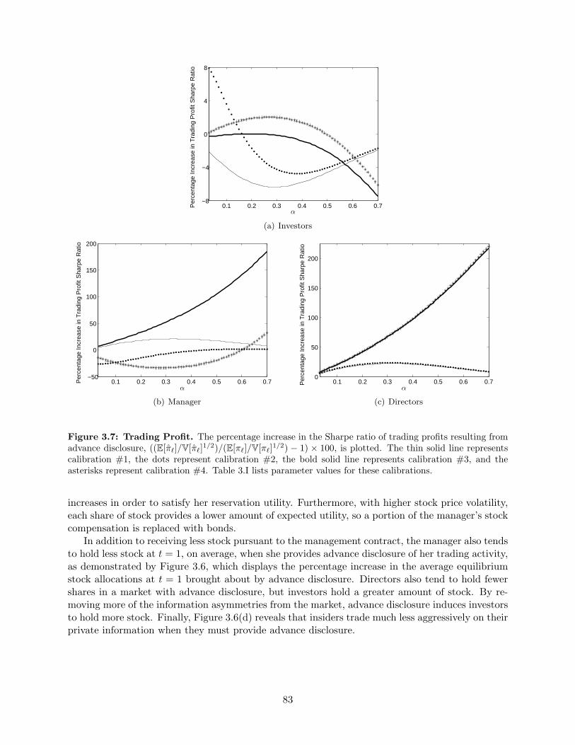
0.1 0.2 0.3 0.4 0.5 0.6 0.7−8

−4

0

4

8

α

Per

cent

age

Incr

ease

in T

radi

ng P

rofit

Sha

rpe

Rat

io

(a) Investors

0.1 0.2 0.3 0.4 0.5 0.6 0.7−50

0

50

100

150

200

α

Per

cent

age

Incr

ease

in T

radi

ng P

rofit

Sha

rpe

Rat

io

(b) Manager

0.1 0.2 0.3 0.4 0.5 0.6 0.70

50

100

150

200

α

Per

cent

age

Incr

ease

in T

radi

ng P

rofit

Sha

rpe

Rat

io

(c) Directors

Figure 3.7: Trading Profit. The percentage increase in the Sharpe ratio of trading profits resulting fromadvance disclosure, ((E[π`]/V[π`]1/2)/(E[π`]/V[π`]1/2) − 1) × 100, is plotted. The thin solid line representscalibration #1, the dots represent calibration #2, the bold solid line represents calibration #3, and theasterisks represent calibration #4. Table 3.I lists parameter values for these calibrations.

increases in order to satisfy her reservation utility. Furthermore, with higher stock price volatility,each share of stock provides a lower amount of expected utility, so a portion of the manager’s stockcompensation is replaced with bonds.

In addition to receiving less stock pursuant to the management contract, the manager also tendsto hold less stock at t = 1, on average, when she provides advance disclosure of her trading activity,as demonstrated by Figure 3.6, which displays the percentage increase in the average equilibriumstock allocations at t = 1 brought about by advance disclosure. Directors also tend to hold fewershares in a market with advance disclosure, but investors hold a greater amount of stock. By re-moving more of the information asymmetries from the market, advance disclosure induces investorsto hold more stock. Finally, Figure 3.6(d) reveals that insiders trade much less aggressively on theirprivate information when they must provide advance disclosure.

83

0.1 0.2 0.3 0.4 0.5 0.6 0.7

0

0.1

0.2

0.3

α

Cer

tain

ty E

quiv

alen

t

(a) Investors

0.1 0.2 0.3 0.4 0.5 0.6 0.7−0.25

−0.2

−0.15

−0.1

−0.05

0

α

Cer

tain

ty E

quiv

alen

t

(b) Directors

Figure 3.8: Welfare. The certainty equivalent of additional consumption without advance disclosurethat is necessary to provide the agents with the same ex ante expected utility that is obtained with advancedisclosure is plotted for various levels of α and multiple calibrations. The thin solid line represents calibration#1, the dots represent calibration #2, the bold solid line represents calibration #3, and the asterisks representcalibration #4. Table 3.I lists parameter values for these calibrations.

3.3.6 Trading Profits

Differences in the stock allocations and the aggressiveness with which insiders trade are bothsignificant factors in the amount of trading profits earned by the agents. We measure tradingprofits as the gain in wealth directly attributable to stock ownership, and it consists of the amountreceived from the terminal payoff at t = 2 plus (minus) any sales (purchases) at t = 1. The tradingprofit for an investor of type `, which is denoted by π`, is given by

π` ≡ S`1Y +(S`0 − S`1

)P (3.70)

for ` ∈ {m, d, i}.Since trading profits are stochastic, it seems natural to evaluate the impact of advance disclosure

on these profits by comparing a Sharpe ratio of trading profits. Specifically, we compute the ratio ofexpected trading profits to the standard deviation of trading profits both with and without advancedisclosure. We then divide this Sharpe ratio with advance disclosure by its counterpart withoutadvance disclosure and subtract one from the resulting fraction. Agents can expect to earn largertrading profits per unit of risk when this metric, which is plotted in Figure 3.7, is positive. Forthe most part, advance disclosure leads to a lower Sharpe ratio of trading profits for investors buta higher Sharpe ratio of trading profits for the manager and directors. However, if we look onlyat the expected trading profits, which are unreported, we observe that the trading profits for themanager and directors fall, on average, with advance disclosure. This finding is consistent withthe post- and pre-announcement results of Huddart, Hughes, and Williams (2010) and Huddart,Hughes, and Levine (2001). We also observe a corresponding rise in the expected trading profitsfor investors.

3.3.7 Welfare

Interestingly, the effect of advance disclosure on the Sharpe ratio of trading profits does notseem to correlate with its effect on welfare. Figure 3.8 measures the change in welfare resulting from

84

0.10.3

0.50.7

02

46

810

0

10

20

30

αθ

Rat

io o

f Effo

rt S

harp

e R

atio

s

Figure 3.9: Managerial Effort. The increase in the Sharpe ratio of managerial effort resulting fromadvance disclosure, (E[(Sm0 +Sm1 )θ2]/V[(Sm0 +Sm1 )θ2]1/2)/(E[(Sm0 +Sm1 )θ2]/V[(Sm0 +Sm1 )θ2]1/2)−1, is plottedfor various values of α and θ. The remaining parameter values are listed in Table 3.I under calibration #1.

advance disclosure. It depicts the certainty equivalent of additional consumption without advancedisclosure necessary to provide the investors and directors with the same ex ante expected utilitythat they obtain with advance disclosure. The manager always receives her reservation expectedutility. Figure 3.8 shows that investors’ ex ante expected utility rises but that directors’ ex anteexpected utility falls with advance disclosure.

3.3.8 Managerial Effort

Advance disclosure can also indirectly affect the manager’s incentives to undertake individuallycostly actions that enhance firm value. Since the manager’s action strategies derived in Section3.2 depend on her stock holdings, it follows that managerial effort itself depends on the manager’sstock holdings. Accordingly, the aggregate effort levels with and without advance disclosure are(Sm0 + Sm1

)θ2 and

(Sm0 + Sm1

)θ2, respectively. Provided that θ 6= 0, advance disclosure results in

greater effort when the manager holds more stock. Firm value is never destroyed through negativeeffort since the manager always holds a non-negative amount of stock.

Because the manager’s stock allocation at t = 1, and hence her effort level, is stochastic anddepends on the realizations of several random variables, we compare effort with advance disclosureto effort without advance disclosure by examining a Sharpe ratio of managerial effort. Figure3.9 plots the percentage increase in the Sharpe ratio of managerial effort resulting from advancedisclosure for various values of α and θ. The figure clearly indicates that the average amount ofeffort per unit of risk increases with advance disclosure, and this increase is more pronounced whenthe insiders possess a great deal of private information. However, the expected effort level falls withadvance disclosure because the manager is granted less stock pursuant the management contractand holds less stock on average after trading at t = 1.

3.3.9 Incentive to Undertake Excessive Risk

Next, we investigate how advance disclosure affects the manager’s incentive to undertake ex-cessive risk for the purpose of generating additional private information. We consider a slightmodification of the model outlined in Section 3.2 that permits the manager to take on additionalrisky projects that have a zero expected payoff. These projects generate more private information

85

0.10.3

0.50.7

0.050.1

0.150.2−8

−6

−4

−2

0

2

x 10−5

αSm0

Ris

k In

cent

ive

Rat

io

Figure 3.10: Risk Incentive. The ratio of the partial derivative of the manager’s ex ante expected utilitywith respect to J1 with advance disclosure to the partial derivative without advance disclosure is plottedover a range of values for α and Sm0 . The remaining parameters are listed in Table 3.I under calibration #1.

but do not create any additional value for the firm on average. We denote the quantity of additionalrisky projects undertaken at time t by Jt and the payoff from these projects by Rt, where Jt ∈ R+

and Rt ∼ N(0, σ2

R

)for t = 1, 2. We further assume that these projects are linearly incorporated

into the stock payoff, which in this setting becomes

˜Y ≡ θ(A1 + A2) + J1R1 + J2R2 + X1 + X2, (3.71)

where a macron ( ) is added to some variables to distinguish them from versions of the modelpreviously discussed. The manager chooses J1 at t = 0 and, along with directors, observes therealization of R1 before trading occurs at t = 1. Investors do not directly observe R1, but they canuse the information available to them in the market to form a conditional distribution of R1. Themanager also selects J2 at t = 1, and R2 is realized at t = 2. Furthermore, R1, R2, X1, X2, k, εm,and εi are mutually independent.

As before, we assume that the stock price and disclosures are linear functions of the insiders’private information, which now includes R1. Hence, the stock price is a linear function of q ≡J1R1 + X1 + ωk in a market without advance disclosure, and the insiders’ trading disclosures arelinear functions of r ≡ J1R1 + X1 + ρhm in a market with advance disclosure. The equilibria arederived in a similar fashion as in Section 3.2, but for the sake of brevity, we do not report theequilibrium outcomes. We note, however, that the action strategies are the same as in Section 3.2while the prices and allocations now incorporate the additional risky projects.

Solving a revised maximization problem for the manager that includes the decision to undertakeadditional risky projects, we find that the manager optimally chooses J2 = 0 both with and withoutadvance disclosure. In both cases, there is no incentive for the manager to create extra risk becauseshe is risk averse and the added uncertainty does not generate more private information on whichshe can capitalize. Conversely, the optimal choice of J1 depends on whether she provides advancedisclosure of her trading activity since the value of the additional private information can potentiallyoutweigh the added risk. Although we are unable to obtain an analytical solution for J1, we cannumerically compute the change in the manager’s ex ante expected utility from a marginal increasein J1 to gauge the manager’s incentive to undertake additional risky projects at t = 0. Figure 3.10plots the ratio of this partial derivative with advance disclosure to the partial derivative withoutadvance disclosure over a range of values for α and Sm0 when J1 = 0. As is evident from the plot,

86

0.10.3

0.50.7

00.05

0.10.15

0.21

1.1

1.2

αSm0

Exp

ecte

d U

tility

Rat

io

Figure 3.11: Expected Utility Ratio. The ratio of the manager’s ex ante expected utility with advancedisclosure to her ex ante expected utility without advance disclosure is plotted over a range of α and Sm0 infigure (a). The remaining parameters are listed in Table 3.I under calibration #1.

the value of the aforementioned ratio is close to zero over the entire range of α and Sm0 , whichmeans that the incentive for the manager to undertake excessive risk is dramatically reduced whenshe must provide advance disclosure of her trading activity.

3.3.10 Voluntary Disclosure

Our final task is to investigate whether the manager would voluntarily commit to provideadvance disclosure of her trading activity in the absence of a requirement to do so. Consistent withHuddart, Hughes, and Williams (2010), we find that she will not. Holding her bond compensationconstant, we compare the manager’s ex ante expected utility with advance disclosure to her exante expected utility without advance disclosure over a range of values for Sm0 and α. Figure 3.11plots a ratio of these utility levels for calibration #1.18 Since agents exhibit CARA preferences,a ratio greater than one indicates a drop in expected utility, and vice versa. It is clear fromthe figure that, given a quantity of future private information and an initial portfolio of stock andbonds, the manager’s expected utility falls when she must provide advance disclosure of her tradingactivity. Hence, the manager will prefer to not commit to advance disclosure after receiving hercompensation package at t = 0, even though she is ex ante indifferent because her compensationpackage is adjusted so that she always receives her reservation utility.

3.3.11 Sensitivity of Results

In this section, we briefly discuss the sensitivity of our results to the realizations of the simulatedvariables. As previously mentioned, we simulate 10,000 realizations each of X1, k, hi, and hm. Tocheck whether this number of realizations provides a sufficient amount of data from which to drawreliable inferences, we group the realizations into 10 buckets of 1,000 realizations each and comparethe simulation results for each bucket. For brevity, we focus on average prices and allocationsbecause they affect many other equilibrium attributes, such as trading profits, welfare, managerialeffort, and the incentive to undertake excessively risky projects. Market-wide equilibrium charac-teristics like market efficiency and liquidity are unaffected by the realizations.

18The other calibrations lead to identical qualitative conclusions.

87

0.1 0.2 0.3 0.4 0.5 0.6 0.70

0.4

0.8

1.2

1.6

α

Per

cent

age

Incr

ease

in A

vera

ge P

rice

(a) Average Price

0.1 0.2 0.3 0.4 0.5 0.6 0.70

1

2

3

4

α

Per

cent

age

Incr

ease

in S

tock

Allo

catio

n

(b) Investors

0.1 0.2 0.3 0.4 0.5 0.6 0.7−10

−8

−6

−4

−2

0

α

Per

cent

age

Incr

ease

in S

tock

Allo

catio

n

(c) Manager

0.1 0.2 0.3 0.4 0.5 0.6 0.7−10

−8

−6

−4

−2

0

α

Per

cent

age

Incr

ease

in S

tock

Allo

catio

n

(d) Directors

Figure 3.12: Sensitivity. The percentage increase in the mean equilibrium price and stock allocationsresulting from advance disclosure is plotted for several simulations of 1, 000 realizations each. The parametervalues are listed in Table 3.I under calibration #1.

Figure 3.12(a) plots the average stock price while Figures 3.12(b)-(d) plot the average equilib-rium stock allocations for 10 different simulations of 1,000 realizations each. As indicated by thefigures, each simulation produces results which are quantitatively similar and qualitatively iden-tical. Therefore, we conclude that 10,000 realizations is a sufficient number to produce reliablesolutions.

3.4 Concluding Remarks

We construct a noisy rational expectations equilibrium model in which informed insiders provideadvance disclosure of their trading activity. Relative to a market in which informed insiders tradewithout providing advance disclosure and investors learn from prices, we find that there are severalbenefits to a market in which investors learn from insiders’ advance disclosures of trades. Inparticular, advance disclosure gives rise to markets that: (i) are informationally more efficient; (ii)are ordinarily more liquid; (iii) have larger managerial effort Sharpe ratios; and (iv) discourage

88

excessively risky projects. A drawback of advance disclosure, however, is that prices are morevolatile. Additionally, there are many consequences of advance disclosure that are neither beneficialnor detrimental. First, prices are higher and risk premiums are smaller, on average, in a market withadvance disclosure. Second, investors tend to hold more stock in equilibrium while insiders tend tohold less. Third, the market value of the manager’s compensation package is higher. Fourth, theSharpe ratio of trading profits may either rise or fall. We also observe that advance disclosure leadsto greater ex ante expected utility for investors but reduced ex ante expected utility for insidersother than the manager. The manager’s expected utility is unaltered in equilibrium because hercompensation package is adjusted. Finally, we find that insiders will not voluntarily commit toprovide advance disclosure of their trading activity.

Our model also presents several interesting avenues for future research. For instance, onecould extend the set of permissible types of trades to include limit orders. The effect of advancedisclosure on independent information acquisition, as in Fishman and Hagerty (1992) or McNicholsand Trueman (1994), is potentially intriguing, as well.

89

Appendix A

The Closed-End Fund Puzzle:Management Fees and PrivateInformation

A.1 Endogenous Stock Price without Liquidity Traders

In this section, we modify our model to allow for an endogenous stock price. We first describethe modifications to our model and present the new equilibrium. We then verify the robustness ofour results.

Modifying our model to allow for an endogenous stock price requires two adjustments to ourset of assumptions. First, we eliminate our assumption that the stock price process is exogenouslygiven by (1.44). Second, to overcome a no-trade theorem that otherwise would prevent tradefrom occurring among the asymmetrically-informed agents, we assume that the investor is slightlyunsophisticated in that he is unable to infer the manager’s private information from the equilibriumstock price. The investor in the modified version of our model has rational expectations in the senseof Muth (1961) and Lucas and Prescott (1971), as he correctly anticipates the distribution of futureasset prices and chooses utility-maximizing portfolios based on his prior information. The only limitto his rationality is that he is unable to “reverse engineer” or invert the price function as in Radner(1979) or Grossman and Stiglitz (1980) to infer the manager’s private information. This is arguablya weaker assumption than the device traditionally used by theorists to overcome no-trade theoremsin a model like ours; namely, noise traders who provide shocks to supply that are completely randomand do not respond in any way to expectations about future prices. Heuristically, this version of ourmodel can be thought of as the limiting case of another variation of our model with an endogenousstock price, fully rational investors, and liquidity traders, which we discuss in Appendix A.2.

Under our new set of assumptions, the endogenously determined equilibrium stock price isequivalent to the exogenous process we assumed for our featured model whenever information issymmetric but not when information is asymmetric. Hence, at the beginning and end of each cyclethe stock price is given by (1.44) and the allocations are given by (1.50) and (1.51). At the middleof cycle n, the manager’s private information is incorporated into the stock price, which is given by

P s3n−1 =3n−2∑τ=1

Xτ +T∑

τ=3n

(µτ − γiγm

Γ σ2τ

)+γiZn,1 + (1− αq)b

(Γµ3n−1 − γiγmσ2

3n−1

)αqγi + (1− αq)Γb

, (A.1)

90

00.25

0.50.75

1

00.25

0.50.75

1

αb

ρ

(a) Issue Premium

00.25

0.50.75

1

00.25

0.50.75

1

αb

E(u

m)


Figure A.1: Issue Premium and Expected Utility.

as well as the stock allocations, which are given by

Sf3n−1 =(Γb− γi)

(Zn,1 − αqµ3n−1

)+ γiγmbσ

23n−1

γmb(αqγi + (1− αq)Γb

)σ2

3n−1

(A.2)

and

Si3n−1 =(Γb− γi)

(αqµ3n−1 − Zn,1 + (1− αq)γmbσ2

3n−1

)γmb

(αqγi + (1− αq)Γb

)σ2

3n−1

. (A.3)

Furthermore, since endogenizing the stock price impacts the extent to which the manager can profitfrom her information advantage, it also affects the discount. The weighted average of the expectedbenefit of the manager’s private information with an endogenous stock price is now given by

δ ≡λ`Υ`

√1− (1−αh)αhγi(Γ+γm)(Γb−γi)2(

γm(αhγi+(1−αh)Γb))2 + λhΥh

√1− (1−α`)α`γi(Γ+γm)(Γb−γi)2(

γm(α`γi+(1−α`)Γb))2

Υ`

√1− (1−αh)αhγi(Γ+γm)(Γb−γi)2(

γm(αhγi+(1−αh)Γb))2 + Υh

√1− (1−α`)α`γi(Γ+γm)(Γb−γi)2(

γm(α`γi+(1−α`)Γb))2 . (A.4)

Accordingly, equilibrium discounts are now described by (1.54), (1.57), and (1.60) with δ in placeof δ.

In summary, the only real difference between the equilibrium in our modified model and in ourfeatured model is the effect of the manager’s information advantage on her portfolio choices wheninformation is asymmetric at the middle of every cycle. With an endogenous stock price, there is aprice feedback effect that limits the manager’s capacity to profit from her information advantage.

We verify the robustness of the results obtained from our featured model in the remainingportion of this appendix. To generate a distribution of discounts that matches empirical observa-tions, we make two minor adjustments to our calibration. First, we set the fixed component of themanagement contract, a, equal to 0.0185. Second, we set the fund’s initial wealth designated forinvestment, Wf , equal to 1.5, which ensures that the fund price does not turn negative in any ofthe simulations. All other parameter values remain the same.

Figure A.1 plots the issue premium and the manager’s ex ante expected utility for various valuesof α and b. Similar to our featured model discussed in Section 1.2, the choice of b that maximizes

91

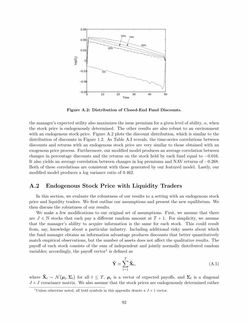
0 10 20 30 40 50−0.09

−0.06

−0.03

0

0.03

0.06

0.09

Time

log(

Dt)

25%

5%

95%

50% 75%

Figure A.2: Distribution of Closed-End Fund Discounts.

the manager’s expected utility also maximizes the issue premium for a given level of ability, α, whenthe stock price is endogenously determined. The other results are also robust to an environmentwith an endogenous stock price. Figure A.2 plots the discount distribution, which is similar to thedistribution of discounts in Figure 1.2. As Table A.I reveals, the time-series correlations betweendiscounts and returns with an endogenous stock price are very similar to those obtained with anexogenous price process. Furthermore, our modified model produces an average correlation betweenchanges in percentage discounts and the returns on the stock held by each fund equal to −0.016.It also yields an average correlation between changes in log premiums and NAV returns of −0.268.Both of these correlations are consistent with those generated by our featured model. Lastly, ourmodified model produces a log variance ratio of 0.462.

A.2 Endogenous Stock Price with Liquidity Traders

In this section, we evaluate the robustness of our results to a setting with an endogenous stockprice and liquidity traders. We first outline our assumptions and present the new equilibrium. Wethen discuss the robustness of our results.

We make a few modifications to our original set of assumptions. First, we assume that thereare J ∈ N stocks that each pay a different random amount at T + 1. For simplicity, we assumethat the manager’s ability to acquire information is the same for each stock. This could resultfrom, say, knowledge about a particular industry. Including additional risky assets about whichthe fund manager obtains an information advantage produces discounts that better quantitativelymatch empirical observations, but the number of assets does not affect the qualitative results. Thepayoff of each stock consists of the sum of independent and jointly normally distributed randomvariables; accordingly, the payoff vector1 is defined as

Y ≡T∑t=1

Xt, (A.5)

where Xt ∼ N(µt,Σt

)for all t ≤ T , µt is a vector of expected payoffs, and Σt is a diagonal

J ×J covariance matrix. We also assume that the stock prices are endogenously determined rather1Unless otherwise noted, all bold symbols in this appendix denote a J × 1 vector.

92

Table A.I: Average Correlation Coefficients.


Fund Returnτ−1 0.504 −0.133Fund Returnτ −0.200Fund Returnτ+1 −0.038

NAV Returnτ−1 0.005 −0.020 −0.021NAV Returnτ 0.345 0.707NAV Returnτ+1 −0.039 0.238

exogenously given by (1.44).Second, to facilitate trade among the rational, asymmetrically informed agents, we assume that

at the middle of every cycle liquidity traders demand a stochastic and unobservable amount of eachstock denoted by kn ∼ N

(0,Σk

)for all n, where 0 is a vector of zeros and Σk is a diagonal J × J

covariance matrix.2 The volatility of liquidity trades is constant across stocks, and σ2k denotes this

volatility for an individual stock. Furthermore, these liquidity shocks are independent across timeand stocks. When solving the model, to maintain tractability we assume that the stock prices atthe middle of cycle n are linear functions of

rn ≡ Zn,1 + (1− αq)γmbΣ3n−1kn. (A.6)

Because kn is unobservable, the stock prices serve as a noisy signal of Zn,1 but do not fully revealits value. However, after observing r through Ps

3n−1, the investor can update his beliefs about Zn,1in a Bayesian fashion to form a posterior of the manager’s private information which is normallydistributed with mean(

αqΣ3n−1 + (1− αq)2γ2mb

2Σ23n−1Σk

)−1αq((1− αq)2γ2

mb2Σ2

3n−1Σkµ3n−1 + Σ3n−1r)

(A.7)

and variance (αqΣ3n−1 + (1− αq)2γ2

mb2Σ2

3n−1Σk

)−1αq(1− αq)2γ2

mb2Σ3n−1Σ2

3n−1Σk. (A.8)

Despite the existence of liquidity traders, the basic techniques described in Section 1.2 can beused to solve this modified version of the model. Since information is symmetric and there areno liquidity trades at the end of each cycle, the equilibrium stock prices at the end of cycle n areanalogous to the stock price in our original model and are given by

Ps3n =

3n−1∑τ=1

Xτ +T∑

τ=3n

(µj,τ −

γiγmΓ Στ1

), (A.9)

where 1 is a vector of ones. Similarly, the stock allocations are given by

Sf3n = γi(Γb)−11 (A.10)

andSi3n = (Γb− γi)(Γb)−11. (A.11)

2Since the sole purpose of the liquidity traders is to generate trade in an environment with asymmetric information,we assume that the liquidity traders do not trade when information is symmetric at the beginning and end of eachcycle. This assumption eliminates unnecessary liquidity trader risk.

93

00.25

0.50.75

1

00.25

0.50.75

1

αb

ρ

(a) Issue Premium

00.25

0.50.75

1

00.25

0.50.75

1

αb

E(u

m)


Figure A.3: Issue Premium and Expected Utility.

The future liquidity trades impact the fund price. In this setting, the weighted average of theinvestor’s expected benefit from the manager’s private information is given by

δ ≡ Jλ`Υ`Φ

−J/2` + λhΥhΦ−J/2h

Υ`Φ−J/2` + ΥhΦ−J/2h

, (A.12)

where

λq ≡αq(1− αq)(1− b)(Γb− γi)σ2

3n−1σ2k

αq + (1− αq)(αqγi(1− b)(Γb− γi + γmb) + (1− αq)γ2

mb2)σ2

3n−1σ2k

(A.13)

and

Φq ≡αq(1− αq)(1− bt)(Γb− γi)σ2

3n−1σ2k

λq(αqΓ + (1− αq)γ2

mb(αqγi + (1− αq)Γb)σ23n−1σ

2k

)2×(αqΓ2 + (1− αq)γ2

mb(2αqγiΓ + (1− αq)Γ2b+ (1− αq)γ2

i γ2mbσ

23n−1σ

2k

)σ2

3n−1σ2k

). (A.14)

The discount at the end of cycle n has a similar form as in our original model and is given by

D3n = a+ b(V3n − V3n−2

)− (N − n)

(δ − a

). (A.15)

The greatest divergence between our original model and our modified model with liquiditytraders occurs at the middle of each cycle. The stock price at the middle of cycle n is given by

Ps3n−1 =

3n−2∑τ=1

Xτ +T∑

τ=3n

(µτ −

γiγmΓ Στ1

)+ θq1 + θq2

(Zn,1 + (1− αq)γmbΣ3n−1kn

), (A.16)

where

θq0 ≡ αqΓI + (1− αq)γ2mb(αqγi + (1− αq)Γb

)Σ3n−1Σk

θq1 ≡ (1− αq)θ−1q0

(αqI + (1− αq)γ2

mb2Σ3n−1Σk

)(Γµ3n−1 − γiγmΣ3n−11

)θq2 ≡ θ−1

q0

(αqΓI + (1− αq)γiγ2

mbΣ3n−1Σk

)94

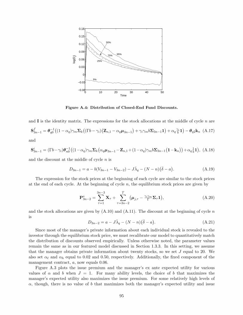
0 10 20 30 40 50−0.06

−0.03

0

0.03

0.06

0.09

0.12

0.15

0.18

Time

log(

Dt)

5%

25%

50%

95%75%

Figure A.4: Distribution of Closed-End Fund Discounts.

and I is the identity matrix. The expressions for the stock allocations at the middle of cycle n are

Sf3n−1 = θ−1q0

((1−αq)γmΣk

((Γb− γi)

(Zn,1 −αqµ3n−1

)+ γiγmbΣ3n−11

)+αq

γib 1)− θq2kn (A.17)

and

Si3n−1 = (Γb−γi)θ−1n0

((1−αq)γmΣk

(αqµ3n−1−Zn,1 +(1−αq)γmbΣ3n−1

(1−kn

))+αq 1

b1), (A.18)

and the discount at the middle of cycle n is

D3n−1 = a− b(V3n−1 − V3n−2)− Jλq − (N − n)(δ − a

). (A.19)

The expression for the stock prices at the beginning of each cycle are similar to the stock pricesat the end of each cycle. At the beginning of cycle n, the equilibrium stock prices are given by

Ps3n−2 =

3n−3∑τ=1

Xτ +T∑

τ=3n−2

(µj,τ −

γiγmΓ Στ1

), (A.20)

and the stock allocations are given by (A.10) and (A.11). The discount at the beginning of cycle nis

D3n−2 = a− Jλq − (N − n)(δ − a

). (A.21)

Since most of the manager’s private information about each individual stock is revealed to theinvestor through the equilibrium stock price, we must recalibrate our model to quantitatively matchthe distribution of discounts observed empirically. Unless otherwise noted, the parameter valuesremain the same as in our featured model discussed in Section 1.3.3. In this setting, we assumethat the manager obtains private information about twenty stocks, so we set J equal to 20. Wealso set α` and αh equal to 0.02 and 0.50, respectively. Additionally, the fixed component of themanagement contract, a, now equals 0.06.

Figure A.3 plots the issue premium and the manager’s ex ante expected utility for variousvalues of α and b when J = 1. For many ability levels, the choice of b that maximizes themanager’s expected utility also maximizes the issue premium. For some relatively high levels ofα, though, there is no value of b that maximizes both the manager’s expected utility and issue

95

Table A.II: Average Correlation Coefficients.


Fund Returnτ−1 0.197 0.016Fund Returnτ −0.152Fund Returnτ+1 −0.170

NAV Returnτ−1 −0.059 −0.004 0.001NAV Returnτ 0.152 0.851NAV Returnτ+1 −0.149 0.196

premium. However, in these cases the utility-maximizing choice of b still leads to relatively largeissue premiums.

The distribution of discounts with liquidity traders is comparable to the distribution fromour featured model and is depicted in Figure A.4. Likewise, the time-series correlations betweendiscounts and returns are also robust to an environment with liquidity traders, as evidenced byTable A.II. Moreover, the average correlation between changes in percentage discounts and thereturns on the stocks held by a fund is −0.054 while the average correlation between changes in logpremiums and NAV returns is −0.199. Finally, the log variance ratio is 0.105.

96

Appendix B

Activist Arbitrage, Lifeboats, andClosed-End Funds

B.1 Discounts and Parameter Values

Table B.I: Summary of Discounts. The appropriate equation for the discount under a variety of cir-cumstances is listed. The “Substitution” column denotes the proper adjustment to make to the superscripton the Dt+1 variable.

SubstitutionScenario Equation Out In

Panel A: Activist and Lifeboat AbsentAll scenarios (2.6) - -

Panel B: Activist Present and Lifeboat AbsentCurrent attempt and Dt ∈ (θκ, κ) (2.9) - -Current attempt and Dt ≤ θκ (2.10) - -Current attempt and Dt ≥ κ (2.10) A ¬ANo attempt and Dt ∈ (θκ, κ) (2.11) - -No attempt and Dt ≤ θκ (2.6) ∅ A

No attempt and Dt ≥ κ (2.6) ∅ ¬A

Panel C: Lifeboat Present and Activist AbsentMDP adopted (2.16) - -MDP not adopted and Dt ∈ (θλ, λ) (2.17) - -MDP not adopted and Dt ≤ θλ (2.6) ∅ δ

MDP not adopted and Dt ≥ λ (2.6) ∅ ¬δ

97

Table B.II: Summary of Discounts with Activist and Lifeboat. The appropriate equation for thediscount under a variety of circumstances is listed. In general, the “Substitution” column denotes theproper adjustment to make to the superscript on the Dt+1 variable. For the case where Dt ∈ (θλ, κ), the“Substitution” column indicates that q should equal zero.

SubstitutionScenario Equation Out In

Panel A: MDP Previously AdoptedCurrent attempt and Dt ∈ (θκ, κ) (2.18) - -Current attempt and Dt ≤ θκ (2.21) - -Current attempt and Dt ≥ κ (2.21) δA δ¬ANo attempt and Dt ∈ (θκ, κ) (2.22) - -No attempt and Dt ≤ θκ (2.16) δ δA

No attempt and Dt ≥ κ (2.16) δ δ¬A

Panel B: MDP Not AdoptedCurrent attempt and Dt ≤ min {θκ, θλ} (2.10) A δA

Current attempt and Dt ∈ (θκ, θλ) (2.9) A δA¬A δ¬A

Current attempt and Dt ∈ (θλ, θκ) (2.19) δ¬A δA¬δA A¬δ

Current attempt and Dt ∈ (κ, θλ) (2.10) A δ¬ACurrent attempt and Dt ∈ (λ, θκ) (2.10) A A¬δCurrent attempt and Dt ∈ (θλ, κ) (2.20) - -Current attempt and Dt ∈ (κ, λ) (2.19) - -Current attempt and Dt ∈ (λ, κ) (2.9) A A¬δ

¬A ¬δACurrent attempt and Dt ≥ max {κ, λ} (2.10) A ¬δANo attempt and Dt ≤ min {θκ, θλ} (2.6) ∅ δA

No attempt and Dt ∈ (θκ, θλ) (2.11) A δA¬A δ¬A

No attempt and Dt ∈ (θλ, θκ) (2.17) δ δA¬δ A¬δ

No attempt and Dt ∈ (κ, θλ) (2.6) ∅ δ¬ANo attempt and Dt ∈ (λ, θκ) (2.6) ∅ A¬δNo attempt and Dt ∈ (θλ, κ) (2.20) q 0No attempt and Dt ∈ (κ, λ) (2.17) δ δ¬A

¬δ ¬δANo attempt and Dt ∈ (λ, κ) (2.11) A A¬δ

¬A ¬δANo attempt and Dt ≥ max {κ, λ} (2.6) ∅ ¬δA

98

Table B.III: Parameter Values.

Variable Symbol ValueTime horizon T 25Expected return µ 0.025Low excess return α` 0High excess return αh 0.1Prior “success” parameter a1 1Prior “failure” parameter b1 1Excess return scale factor γ1 1Management fee φ 0.02Excess return adjustment threshold Υ 0.023775Cost of attack c 0.04Probability of liquidation q 0.60Liquidation probability scale factor σ 1/9Liquidation probability scale factor η 2/3Dividend rate δ 0.09Lifeboat trigger λ 0.90Approval threshold θλ 0.80

B.2 Proofs

Proof of Proposition 1. At every point in time, the expected return for the fund must equal themarket expected rate of return. Therefore,

1 + µ = Et

[Rft+1

]= Et

[Pt+1

]/Pt

= Et

[Dt+1Vt+1

]/Pt

= Et

[Dt+1 (M + αt+1)

]Vt/Pt,

which can be solved for Dt to obtain the desired result. The second equality follows from (2.5),the third equality follows from (2.2), and the final equality follows from (2.3) and the lack of serialcorrelation and cross-correlation between the return on the fund’s portfolio and the excess returngenerated by the fund manager.

99

Proof of Proposition 2. At every point in time, the expected return for the fund must equal themarket expected rate of return. Therefore,

1 + µ = Et

[Rft+1

]= Et

[Pt+1

]/Pt

=q

PtEt

[Vt+1

]+

1− qPt

(ρκEt

[DAt+1Vt+1

]+ (1− ρκ)Et

[D¬At+1Vt+1

])(B.1)

= qVtPtEt [M + γtαt+1] + (1− q) Vt

Pt

(κ−Dt

κ− θκEt

[DAt+1 (M + γtαt+1)

]+Dt − θκκ− θκ

Et

[D¬At+1 (M + γtαt+1)

]),

which can be solved for Dt to obtain the desired result. The third equality follows from (2.2) whilethe final equality follows from (2.7), (2.8), and the lack of serial correlation and cross-correlationbetween the return on the fund’s portfolio and the excess return generated by the fund manager.

Proof of Proposition 3. At every date, the expected return on the fund must equal the marketexpected rate of return. For (i), this implies

1 + µ = Et

[Rft

]= Et

[Pt+1 + dt+1

]/Pt

= Et

[Dδt+1Vt+1 + dt+1

]/Pt

=VtPtEt

[Dδt+1 (M + γtαt+1 − δ) + δ

],

which can be solved for Dt to obtain the desired result. The second equality follows from (2.15),the third equality follows from (2.2), and the final equality follows from (2.12), (2.13), and the lackof serial correlation and cross-correlation between the return on the fund’s portfolio and the excessreturn generated by the fund manager.

Similarly, the implication for (ii) is

1 + µ = Et

[Rft

]= Et

[Pt+1

]/Pt

=ρλPtEt

[Dδt+1Vt+1

]+

1− ρλPt

Et

[D¬δt+1Vt+1

](B.2)

=VtPt

(λ−Dt

λ− θλEt

[Dδt+1 (M + γtαt+1)

]+Dt − θλλ− θλ

Et

[D¬δt+1 (M + γtαt+1)

]),

which can solved for Dt to obtain the desired result. The third equality follows from (2.2) whilethe final equality follows from (2.3), (2.14), and the lack of serial correlation and cross-correlationbetween the return on the fund’s portfolio and the excess return generated by the fund manager.

100

Proof of Proposition 4. At every date, the expected return for the fund must equal the marketexpected rate of return. For (i), this implies

1 + µ = Et

[Rft+1

]= Et

[Pt+1 + dt+1

]/Pt

=q

PtEt

[Vt+1 + dt+1

]+

1− qPt

(ρκEt

[DδAt+1Vt+1 + dt+1

]+ (1− ρκ)Et

[Dδ¬At+1 Vt+1 + dt+1

] )(B.3)

= δVtPt

+ qVtPtEt [M + γtαt+1 − δ]

+ (1− q) VtPt

(κ−Dt

κ− θκEt

[DδAt+1 (M + γtαt+1 − δ)


Et

[Dδ¬At+1 (M + γtαt+1 − δ)

]),

which can be solved for Dt to obtain the desired result. The second equality follows from (2.15),the third equality follows from (2.2) while the final equality follows from (2.8), (2.12), (2.13) andthe lack of serial correlation and cross-correlation between the return on the fund’s portfolio andthe excess return generated by the fund manager.

The implication for (ii) is

1 + µ = Et

[Rft+1

]= Et

[Pt+1

]/Pt

=q

PtEt

[Vt+1

]+

1− qPt

(ρλEt

[Dδ¬At+1 Vt+1

]+ (1− ρλ)Et

[D¬δAt+1 Vt+1

])(B.4)

= qVtPtEt [M + γtαt+1] + (1− q) Vt

Pt

(λ−Dt

λ− θλEt

[Dδ¬At+1 (M + γtαt+1)

]+Dt − θλλ− θλ

Et

[D¬δAt+1 (M + γtαt+1)

]),

which can be solved for Dt to obtain the desired result. The second equality follows from (2.5), thethird equality follows from (2.2) and (2.7) while the final equality follows from (2.3), (2.14), andthe lack of serial correlation and cross-correlation between the return on the fund’s portfolio andthe excess return generated by the fund manager.

101

For (iii),

1 + µ = Et

[Rft+1

]= Et

[Pt+1

]/Pt

=q

PtEt

[Vt+1

]+

1− qPt

[ρλ

(ρκEt

[DδAt+1Vt+1

]+ (1− ρκ)Et

[Dδ¬At+1 Vt+1

])+ (1− ρλ)

(ρκEt

[DA¬δt+1 Vt+1

]+ (1− ρκ)Et

[D¬δAt+1 Vt+1

]) ]= q

VtPtEt [M + γtαt+1]

+ (1− q) VtPt

[λ−Dt

λ− θλ

(κ−Dt

κ− θκEt

[DδAt+1 (M + γtαt+1)


Et

[Dδ¬At+1 (M + γtαt+1)

])+Dt − θλλ− θλ

(κ−Dt

κ− θκEt

[DA¬δt+1 (M + γtαt+1)


Et

[D¬δAt+1 (M + γtαt+1)

])],

which can be rearranged to obtain xD2t + yDt + z = 0, where x, y, and z are defined in the

Proposition. The second equality follows from (2.5), the third equality follows from (2.2) and (2.7)while the final equality follows from (2.3), (2.8), (2.14), and the lack of serial correlation and cross-correlation between the return on the fund’s portfolio and the excess return generated by the fundmanager.

102

Appendix C

Advance Disclosure of Insider Trading

Proof of Corollary 1. Without advance disclosure,

Σ =(V[Y |P

])−1

=(V[θ2Sm1 + X1 + X2|P

])−1

=(

γ2σ21σ

42σ

2kσ

2ε

(1 +Nd)2σ21

(σ2k + σ2

ε

)+ σ2

kσ2ε

(γσ2

2 − θ2)2 + σ2

2

)−1

=Γ3

Γ4σ22

,

where the second equality follows from (3.1), (3.15), and the fact that Sm1 is a function of X1, thethird equality follows from (3.16) and (3.22), and the last equality is a product of algebra.

On the other hand, with advance disclosure,

Σ =(V[ ˜Y |Sm1

])−1

=(V[X1 + X2|Sm1

])−1

=(

ρ2σ21σ

2ε

σ21 + ρ2σ2

ε

+ σ22

)−1

=σ2

1 + ρ2σ2ε

ρ2σ21σ

2ε +

(σ2

1 + ρ2σ2ε

)σ2

2

,

where the second equality follows from (3.1) and the fact that Sm1 is observed by the market, thethird equality follows from from (3.52), and the last equality is a consequence of algebra.

Proof of Corollary 2. To find the expected payoff without advance disclosure, we substitute themanager’s action strategy, (3.15), and stock holdings, (3.8), into the stock payoff, (3.1), and inte-grate over X2. We then subtract the stock price, (3.6), substitute (3.4) for hi, and integrate overX1, k, and εi to obtain the average risk premium, which is given by (3.66). Likewise, the averagerisk premium with advance disclosure is derived by first substituting (3.35) and (3.42) into (3.1)and integrating over X2. Then, (3.33) is subtracted, (3.3) is substituted for hm, and the resultingexpression is integrated over X1, k, and εm, yielding (3.67).

Proof of Corollary 3. The expressions follow immediately from substituting hi = k + εi into (3.6)and hm = k + εm into (3.33) and differentiating with respect to k.

103

Bibliography

Admati, Anat R. and Paul Pfleiderer. 1991. “Sunshine Trading and Financial Market Equilibrium.” Review ofFinancial Studies 4 (3):443–481.

Arora, Navneet, Nengjiu Ju, and Hui Ou-Yang. 2003. “An Agency Explanation of the Closed-End Fund Puzzles.”Working Paper, University of Maryland.

Ausubel, Lawrence M. 1990. “Insider Trading in a Rational Expectations Economy.” American Economic Review80 (5):1022–1041.

Babenko, Ilona and Rik Sen. 2011. “Do Non-Executive Employees Have Information? Evidence from Employee StockPurchase Plans.” Arizona State University.

Barclay, Michael J., Clifford G. Holderness, and Jeffrey Pontiff. 1993. “Private Benefits from Block Ownership andDiscounts on Closed-End Funds.” Journal of Financial Economics 33 (3):263–291.

Bebchuk, Lucian and Jesse Fried. 2009. “Taming the Stock Option Game.” Project Syndicate November.

Berk, Jonathan B. and Richard C. Green. 2004. “Mutual Fund Flows and Performance in Rational Markets.” Journalof Political Economy 112 (6):1269–1295.

Berk, Jonathan B. and Richard Stanton. 2007. “Managerial Ability, Compensation, and the Closed-End FundDiscount.” Journal of Finance 62 (2):529–556.

Bhattacharya, Utpal and Matthew Spiegel. 1991. “Insiders, Outsiders, and Market Breakdowns.” Review of FinancialStudies 4 (2):255–282.

Bond, Philip, Itay Goldstein, and Edward Simpson Prescott. 2010. “Market-Based Corrective Actions.” Review ofFinancial Studies 23 (2):781–820.

Bonser-Neal, Catherine, Greggory Brauer, Robert Neal, and Simon Wheatley. 1990. “International InvestmentRestrictions and Closed-End Country Fund Prices.” Journal of Finance 45 (2):523–547.

Boudreaux, Kenneth J. 1973. “Discounts and Premiums on Closed-End Mutual Funds: A Study in Valuation.”Journal of Finance 28 (2):515–522.

Bradley, Michael, Alon Brav, Itay Goldstein, and Wei Jiang. 2010. “Activist Arbitrage: A Study of Open-EndingAttempts of Closed-End Funds.” Journal of Financial Economics 95 (1):1–19.

Brauer, Greggory A. 1984. “‘Open-Ending’ Closed-End Funds.” Journal of Financial Economics 13 (4):491–507.

———. 1988. “Closed-End Fund Shares’ Abnormal Returns and the Information Content of Discounts and Premi-ums.” Journal of Finance 43 (1):113–127.

Brav, Alon, Wei Jiang, Frank Partnoy, and Randall Thomas. 2008. “Hedge Fund Activism, Corporate Governance,and Firm Performance.” Journal of Finance 63 (4):1729–1775.

Brickley, James, Steven Manaster, and James Schallheim. 1991. “The Tax-timing Option and the Discounts onClosed-End Investment Companies.” Journal of Business 64 (3):287–312.

Brickley, James A. and James S. Schallheim. 1985. “Lifting the Lid on Closed-End Investment Companies: A Caseof Abnormal Returns.” Journal of Financial and Quantitative Analysis 20 (1):107–117.

104

Chan, Justin, Ravi Jain, and Yihong Xia. 2005. “Market Segmentation, Liquidity Spillover, and Closed-end CountryFund Discounts.” Working Paper, University of Pennsylvania.

Chay, J.B. and Charles A. Trzcinka. 1999. “Managerial Performance and the Cross-sectional Pricing of Closed-endFunds.” Journal of Financial Economics 52 (3):379–408.

Chen, Nai-Fu, Raymond Kan, and Merton H. Miller. 1993. “Are the Discounts on Closed-End Funds a SentimentIndex?” Journal of Finance 48 (2):795–800.

Cherkes, Martin, Jacob Sagi, and Richard Stanton. 2009. “A Liquidity-Based Theory of Closed-End Funds.” Reviewof Financial Studies 22 (1):257–297.

Cherkes, Martin, Jacob S. Sagi, and Jay Wang. 2009. “A Neoclassical Model of Managed Distribution Plans: Theoryand Evidence.” Working Paper, Columbia University.

Choi, Stephen J., Jill E. Fisch, and Marcel Kahan. 2009. “Director Elections and the Role of Proxy Advisors.”Southern California Law Review 82:649–702.

Chopra, Navin, Charles M. C. Lee, Andrei Shleifer, and Richard H. Thaler. 1993. “Yes, Discounts on Closed-EndFunds Are a Sentiment Index.” Journal of Finance 48 (2):801–808.

Cohen, Lauren, Christopher Malloy, and Lukasz Pomorski. 2012. “Decoding Inside Information.” Journal of Finance,forthcoming.

Coles, Jeffrey L., Jose Suay, and Denise Woodbury. 2000. “Fund Advisor Compensation in Closed-End Funds.”Journal of Finance 55 (3):1385–1414.

Curtis, James M. and Robert A. Robertson. 2008. “Special Duties of Closed-End Fund Directors.” In Fund Gover-nance: Legal Duties of Investment Company Directors, edited by Robert A. Robertson. Law Journal Press.

De Long, J. Bradford, Andrei Shleifer, Lawrence H. Summers, and Robert J. Waldmann. 1990. “Noise Trader Riskin Financial Markets.” Journal of Political Economy 98 (4):703–738.

Deaves, Richard and Itzhak Krinsky. 1994. “A Possible Reconciliation of Some of the Conflicting Findings on Closed-End Fund Discounts: A Note.” Journal of Business Finance and Accounting 21 (7):1047–1057.

Del Guercio, Diane, Larry Y. Dann, and M. Megan Partch. 2003. “Governance and Boards of Directors in Closed-EndInvestment Companies.” Journal of Financial Economics 69 (1):111–152.

DeMarzo, Peter M., Michael J. Fishman, and Kathleen M. Hagerty. 1998. “The Optimal Enforcement of InsiderTrading Regulations.” Journal of Political Economy 106 (3):602–632.

Dimson, Elroy and Carolina Minio-Kozerski. 1999. “Closed-End Funds: A Survey.” Financial Markets, Institutionsand Instruments 8 (2):1–41.

Edmans, Alex, Itay Goldstein, and Wei Jiang. 2012. “The Real Effects of Financial Markets: The Impact of Priceson Takeovers.” Journal of Finance, forthcoming.

Elton, Edwin J., Martin J. Gruber, and Jeffrey A. Busse. 1998. “Do Investors Care about Sentiment?” Journal ofBusiness 71 (4):477–500.

Fama, Eugene F. and Kenneth R French. 2010. “Luck versus Skill in the Cross-Section of Mutual Fund Returns.”Journal of Finance 65 (5):1915–1947.

Fishman, Michael J. and Kathleen M. Hagerty. 1992. “Insider Trading and the Efficiency of Stock Prices.” RANDJournal of Economics 23 (1):106–122.

Fried, Jesse M. 1998. “Reducing the Profitability of Corporate Insider Trading through Pretrading Disclosure.”Southern California Law Review 71:303–392.

———. 2006. “Advance Disclosure of Managers’ Stock Trades: A Proposal to Improve Executive Compensation.”The Economists’ Voice 3 (8). Article 7.

105

Gemmill, Gordon and Dylan C. Thomas. 2002. “Noise Trading, Costly Arbitrage, and Asset Prices: Evidence fromClosed-End Funds.” Journal of Finance 57 (6):2571–2594.

Glode, Vincent. 2011. “Why Mutual Funds ‘Underperform’.” Journal of Financial Economics 99 (3):546–559.

Grossman, Sanford J. and Oliver D. Hart. 1980. “Takeover Bids, the Free-Rider Problem, and the Theory of theCorporation.” Bell Journal of Economics 11 (1):42–64.

Grossman, Sanford J. and Joseph E. Stiglitz. 1980. “On the Impossibility of Informationally Efficient Markets.”American Economic Review 70 (3):393–408.

Hamilton, James D. 1994. Time Series Analysis. Princeton University Press.

Harris, Milton and Bengt Holmstrom. 1982. “A Theory of Wage Dynamics.” Review of Economic Studies 49 (3):315–333.

Hermalin, Benjamin E. and Michael S. Weisbach. 2012. “Information Disclosure and Corporate Governance.” Journalof Finance 67 (1):195–234.

Huddart, Steven, John S. Hughes, and Carolyn B. Levine. 2001. “Public Disclosure and Dissimulation of InsiderTrades.” Econometrica 69 (3):665–681.

Huddart, Steven, John S. Hughes, and Michael Williams. 2010. “Pre-Announcement of Insiders’ Trades.” Pennsyl-vania State University.

Jagolinzer, Alan D. 2009. “SEC Rule 10b5-1 and Insiders’ Strategic Trade.” Management Science 55 (2):224–239.

Jensen, Michael C. 1968. “The Performance of Mutual Funds in the Period 1945-1964.” Journal of Finance 23 (2):389–416.

Johnson, Shane A., Ji-Chai Lin, and Kyojik Roy Song. 2006. “Dividend Policy, Signaling, and Discounts on Closed-End Funds.” Journal of Financial Economics 81 (3):539–562.

Kim, Chang-Soo. 1994. “Investor Tax-Trading Opportunities and Discounts on Closed-End Mutual Funds.” Journalof Financial Research 17 (1):65–75.

Klein, Michael R. 1983. “Outsider Proposes Changes in Insider Trading Bill.” Legal Times, December 8th.

Kumar, Raman and Gregory M. Noronha. 1992. “A Re-Examination of the Relationship Between Closed-End FundDiscounts and Expenses.” Journal of Financial Research 15 (2):139–147.

Kyle, Albert S. 1985. “Continuous Auctions and Insider Trading.” Econometrica 53 (6):1315–1335.

Lee, Charles M. C., Andrei Shleifer, and Richard H. Thaler. 1990. “Closed-End Mutual Funds.” Journal of EconomicPerspectives 4 (4):153–164.

———. 1991. “Investor Sentiment and the Closed-End Fund Puzzle.” Journal of Finance 46 (1):75–109.

Leland, Hayne E. 1992. “Insider Trading: Should It Be Prohibited?” Journal of Political Economy 100 (4):859–887.

Lenkey, Stephen L. 2011. “Activist Arbitrage, Lifeboats, and Closed-End Funds.” Working Paper, Carnegie MellonUniversity.

Lucas, Robert E. and Edward C. Prescott. 1971. “Investment Under Uncertainty.” Econometrica 39 (5):659–681.

Malkiel, Burton G. 1977. “The Valuation of Closed-End Investment-Company Shares.” Journal of Finance 32 (3):847–859.

McNichols, Maureen and Brett Trueman. 1994. “Public Disclosure, Private Information Collection, and Short-TermTrading.” Journal of Accounting and Economics 17 (1):69–94.

Muth, John F. 1961. “Rational Expectations and the Theory of Price Movements.” Econometrica 29 (3):315–335.

106

Oh, Gyutaeg and Stephen A. Ross. 1994. “Asymmetric Information and the Closed-End Fund Puzzle.” The WhartonFinancial Institutions Center Working Paper 94-19.

Peavy, John W. III. 1990. “Returns on Initial Public Offerings of Closed-End Funds.” Review of Financial Studies3 (4):695–708.

Pontiff, Jeffrey. 1995. “Closed-End Fund Premia and Returns Implications for Financial Market Equilibrium.” Journalof Financial Economics 37 (3):341–370.

———. 1997. “Excess Volatility and Closed-End Funds.” American Economic Review 87 (1):155–169.

Radner, Roy. 1979. “Rational Expectations Equilibrium: Generic Existence and the Information Revealed by Prices.”Econometrica 47 (3):655–678.

Roenfeldt, Rodney L. and Donald L. Tuttle. 1973. “An Examination of the Discounts and Premiums of Closed-EndInvestment Companies.” Journal of Business Research 1 (2):129–140.

Ross, Stephen A. 2002a. “Neoclassical Finance, Alternative Finance and the Closed End Fund Puzzle.” EuropeanFinancial Management 8 (2):129–137.

———. 2002b. “A Neoclassical Look at Behavioral Finance.” Working Paper, The Princeton Lectures in FinanceIII.

Roulstone, Darren T. 2001. “The Relation Between Insider-Trading Restrictions and Executive Compensation.”Journal of Accounting Research 41 (3):525–551.

Samuelson, S. S. 1988. “The Prevention of Insider Trading: A Proposal for Revising Section 16 of the SecuritiesExchange Act of 1934.” Harvard Journal on Legislation 25 (2):511–531.

Spiegel, Matthew and Avanidhar Subrahmanyam. 1992. “Informed Speculation and Hedging in a NoncompetitiveSecurities Market.” Review of Financial Studies 5 (2):307–329.

Thompson, Rex. 1978. “The Information Content of Discounts and Premiums on Closed-End Fund Shares.” Journalof Financial Economics 6 (2):151–186.

Wang, Z. Jay and Vikram Nanda. 2008. “Why Do Aggressive Payout Policies Reduce Fund Discounts - Is It Signaling,Agency Costs, or Dividend Preferences?” Working Paper, University of Illinois.

Weiss, Kathleen. 1989. “The Post-Offering Price Performance of Closed-End Funds.” Financial Management18 (3):57–67.

Wermers, Russ, Youchang Wu, and Josef Zechner. 2008. “Portfolio Performance, Discount Dynamics, and theTurnover of Closed-End Fund Managers.” Working Paper, University of Maryland.

107

Essays on Closed-End Funds and Advance Disclosure of Trading

Documents

Transcript of Essays on Closed-End Funds and Advance Disclosure of Trading