U n i v e r s i t a t A u t ò n o m a d e B a r c e l o n a

F a c u l t y o f S o c i a l S c i e n c e s a n d L a w , D e p a r t m e n t o f B u s i n e s s a n d E c o n o m i c s

P h D i n A p p l i e d E c o n o m i c s

E S S A Y S I N M A R K E T C O N N E C T E D N E S S

Chapte r 1

Market Connectedness : Methodo logy on Sp i l l ove r

and F low o f In fo rmat ion w i th Return and Vo la t i l i t y Se r i es

Chapte r 2

Turk ish and In te rnat iona l S tock Marke ts :

A Network Pe rspect ive

Chapte r 3

The Russ ian s tock marke t

dur ing the Ukra in ian Cr is is : A Network Pe rspect ive

N A R O D E R K O L

May , 2016

Superv iso rs :Hara ld Schmidbauer

Jav ie r Asens io

Chapter 1:

Market Connectedness: Methodology on

Spillover and Flow of Information with

Return and Volatility Series∗

May 27, 2016

Abstract

The goal of the present study is to investigate the market connectedness and

offers an extended methodology by using return and return volatility series. The

spillover methodology developed by Diebold and Yilmaz (2009) will be combined

with the focus of flow of information and by using return and return volatility series

we quantify dynamically the amount of market connectedness and analyse different

interpretations of connectedness that comes from either using the expectation of

stock market prices or using the variations of them.

At this point, our study have another purpose. Because we need the volatil-

ity series of stock markets to apply the methodology, we extend the German and

Klass (1980) volatility estimation method and explain the intuition behind it. We

compare two methodologies for estimating the volatility series; extension of Ger-

man and Klass (1980) and GARCH approach. Volatility spillovers differs in terms

of the estimation methodology we have used and we examine the advantages for

each method. For these purpose, we use the stock market data of Systemic five

countries which are; Dow Jones Industrial Average (USA, New York Stock Ex-

change), FTSE (UK, London Stock Exchange), DAX (Germany, Frankfurt Stock

Exchange), CAC40 (France, Euronext Paris), Nikkei 225 (Japan, Tokyo Stock Ex-

change) and we add RTS (Russia, Russian Stock Index) for the part of our study

and interpret the results.

∗This research have been submitted and presented on the International Conference of Ecomod 2015,

held in Boston, United States. The paper is published in: EcoMod Network (ed.), Proceedings of the

International Conference on Policy Modelling EcoMod 2015 , Boston, United States, July 2015.

1

1 Introduction

Economic entities are becoming more and more interconnected with each other and the

overall degree of international equity market connectedness has been increasing espe-

cially over the past two decades. Although, there is an evidence that there is a strong

connection among markets, new approaches of measuring and quantifying the connection

and understanding its dynamics are still being developed.

To measure the connection among countries a notion of contagion should be referred

to. In the 1990s many experts think that contagion should only be taken into account

in case of an emerging markets and it is an issue of the past only. But, when currency

devaluations in many countries in the world, for example Thailand’s 1997, Russia’s 1998

and Turkish financial crisis in 2001 1, have started to affect global financial markets

and contagion became very important issue and entered to the mainstream economic

terminology 2. Dornbusch et al. (2000) defined the contagion “the spread of market

disturbances from one country to the other ”.

There are many contagion definitions in the literature and all offer their own method-

ology to quantify it. Karolyi (2003) and Dungey et al. (2005) examine the surveys of def-

initions and classifications of contagion in their study. According to World Bank3, “Con-

tagion is the cross-country transmission of shocks or the general cross-country spillover

effects. Contagion can take place both during “good” times and “bad” times. Then,

contagion does not need to be related to crises. However, contagion has been emphasized

during crisis times.” Gallo and Otranto (2008) discuss the concepts of “spillover”, “con-

tagion” and “interconnectedness” in their study which are generally used synonymously

and they establish some practical definitions for them.

Another concept which is very similar to contagion is the “spillover” which started

to become a known terminology after the crash of global markets in October 1987. King

et al. (1990) investigate the reason of the collapse of world markets in October 1987 and

refer to the spillover idea. Hamao, Masulis and Ng (1990) examine the price changes and

price volatilities of Tokyo, London and New York stock markets. Another example of

an analysis in spillovers is the study of Susmel and Engle (1994) who analyse the return

and volatility spillovers between the equity markets of New York and London.

Starting from the October 1987 crisis, the literature of investigation on spillovers

within developed economies has improved. Baur and Jung (2006) analyse return and

volatility spillovers between US and German stock markets, similarly, Golosnoy, Gribisch

and Liesenfeld (2015) measure intra-daily volatility spillovers before and during the

subprime crisis in US, German and Japanese stock markets. On the other hand, the lit-

erature to understand spillovers among developed and emerging economies is still being

developed and after the 90s where crisis from emerging economies started to affect the

1Didier et al. (2008) and Pinto and Ulatov (2010) offered detailed information about the currency

devaluations in many countries in their study.2See Forbes for further information3See http://go.worldbank.org/JIBDRK3YC0, retrieved 2014-04-22

2

whole world and the literature related with this issue is gradually increasing. For exam-

ple, Bekiros (2014) investigates volatility spillovers of the US, EU and BRIC markets.

Balli et al. (2015) analyse the return and volatility spillovers from developed markets to

emerging markets from Asia, Middle East and North Africa region countries.

As we have mentioned above, contagion does not necessarily means a “bad” effect

of an event to the other but the perception is generally in that direction. The concept

of interconnectedness identify all this good and bad effects and explains more than

contagion.4 Diebold and Yilmaz (2014) examine the connectedness of major US financial

institutions stock return volatilities; Choudhry and Jayasekera (2014), investigate the

impact of the 2008 global crisis on spillovers in the European banking industry. Bubak et

al. (2011) analyse volatility spillovers between Central European and EUR/USD foreign

exchange markets; Hou (2013) examine the spillover effects from the interest rate market

to equity markets in euro area.

Also, a literature on event study analysis exists where the aim is to find a link among

certain political or economic events and economic entities. For instance, Mutan et al.

(2009) evaluate the impact of various 10 events from 1990 to 2008 including economic,

political events, terrorism and natural disaster on the economy of Turkey. The literature

can be enlarge and many researches can be counted here but since all looks at markets

in isolation and they do not cover the network perspective, it is beyond the scope of the

present study because they tell less than what we aim to do.

We measure the connectedness using the stock market data because of the advantages

to analyse the economic links between two countries on the basis of stock market data,

rather than aggregate economic data published by national statistical offices, is that

stock market data are readily available, allowing analysis in almost real time.

To measure the connectedness, we have three different purposes for this paper. First,

we measure the connectedness of different stock markets using return spillovers by the

methodology of Diebold and Yilmaz (2009). The contribution in this case, will be not

only looking on the return spillovers but also develop a methodology to measure the

connectedness by using volatility-to-volatility spillovers. The details of the method will

be explained in the following sections of this paper. But for now, we emphasize that to

compute the volatility spillovers we need the weekly volatility series of each market. To

do this, we develop a methodology to obtain the weekly volatility series using the German

and Klass (1980) methodology. Below, we will explain the objective of this methodology

and the intuition behind it.

One of the approach to measure equity market connectedness, which we mentioned

above, is based on forecast error variance decomposition, developed by Diebold and Yil-

maz (2009), and we will discuss the extension of this approach to assess the propagation

of information across markets.

4See Forbes (2012) for further information.

3

One way to quantify market connectedness is to estimate the variance of the error

when forecasting future return or return volatilities on the asset price. Diebold and

Yilmaz (2009, 2013) use this idea to develop a network view of markets as nodes and

weights determined by variance shares. They decompose the error variances of joint

asset return forecasts, using the vector autoregressive (VAR) models. In terms of their

approach, the decomposed error variances present a network with assets as nodes and the

weights of links between nodes determined by shares of forecast error variance spillovers.

Using this methodology, pairwise spillovers can be discussed, but their goal is to go one

step further and designate the degree of market connectedness. They suggest a measure

for the degree of market connectedness which they call the spillover index.

Schmidbauer et al. (2012) extend the spillover index methodology and quantify dy-

namically the amount of connectedness of markets with a focus on the flow of infor-

mation. They use the concepts of Kullback-Leibler divergence developed by Demetrius

(1974) and Tuljapurkar (1982) to measure the amount of market connectedness dynam-

ically. Schmidbauer et al. (2012) discuss the Kullback-Leibler divergence in the field of

market connectedness and define the relative market entropy approach. First market

entropy, measures the amount of information created every period, and the second one

quantifies the speed of information digestion in the system. Building on the framework

developed by Diebold and Yilmaz (2009), they construct supplementary measures of

market connectedness using information theory and population dynamics.

The first purpose of the present paper is to use these two methodologies developed

by Diebold and Yilmaz (2009) and Schmidbauer et al. (2012) with weekly return and

weekly return volatility series and to interpret the different and similar outcomes of

market connectedness in the case of using the expectation and the standard deviation of

assets. The main goal is to analyse the market with respect to different structures, in our

case, using the expectation of the prices and plus using the variations of them as a data.

Using the spillover and entropy approach, we want to compare the results of market

connectedness while return series is used and on the other hand, return volatility series

is used instead of return. Analysing not only the return series but also the variations

of them will give us an information about how do they complement each other. So, the

main goal is to quantify dynamically the amount of connectedness of markets with a

focus on the spillover and the flow of information and apply the methodologies using

weekly return and weekly return volatility data. Therefore, this will give a chance to

analyze different interpretations of market connectedness that comes from either using

the expectation of the prices or using the variations of them.

As it will be explained in Section 3.1.1, to compute the volatility spillovers we need

to obtain the weekly volatility series. We developed a methodology using the Brownian

motions idea. We simulate brownian motions to have an intuition for the estimation

of volatility series. Rather than the German and Klass (1980) approach, we have also

calculated the volatility spillover using daily volatility data estimated by the GARCH

methodology. One of the purpose of this study is to compare the methodologies of

volatility estimation and find the suitable one for our study. In the Empirical part, we

4

compared the German and Klass and GARCH approach and analyse them in terms of

volatility spillovers.

The data that we used in this study divided into two parts to measure the connect-

edness with respect to two different goals. The first method used in the present paper

is illustrated using data from the stock markets of five countries : Dow Jones Industrial

Average (USA, New York Stock Exchange), FTSE (UK, London Stock Exchange), DAX

(Germany, Frankfurt Stock Exchange), CAC40 (France, Euronext Paris), Nikkei 225

(Japan, Tokyo Stock Exchange). The weekly return and weekly return volatility data

are used to apply spillover and entropy methodologies.

The second one, uses daily closing quotations of the Russian stock index and the

five stock indices representing stock markets in the “Systemic Five” countries. We will

compute return spillovers using the same methodology with the first data set, but for

the volatility spillovers we will use the GARCH methodology instead of the German and

Klass.

R-project (R (2015)) is used to apply the methodologies for both return and return

volatility data. Using again R-project, an automatic update system code has written

by us and uploaded to the website of http://financialnetworks.eu/ which updates

automatically the spillovers and flow of information and plots the updated figures each

day. For now, we constructed four sets of networks using different number of stock

market prices and compute the spillovers and propagation values separately. The detailed

information about the methodology will be provided in the paper.

This paper is organized as follows. Section 2, describes the methodologies of return

spillovers and entropy. It is a review of the spillover methodology developed by Diebold

and Yilmaz (2009) and entropy methodology. Section 3 is the methodology of volatility

spillovers which we develop and KLIC and KS entropy using volatility series. The method

of obtaining volatility is explained using the idea developed by German and Klass (1980).

The intuition of estimating the volatility series is explained in detail in this section.

We have also explained the GARCH methodology of estimating the volatility series.

Section 4 describes some properties of the two groups of data and explains how to

obtain the weekly/daily return and weekly/daily volatility series. Empirical results of

the two methodologies, explained in Section 2 and 3, are presented in Section 5 for

both spillovers and entropy and with two estimation methodology of volatility spillovers

and the comparison of them. Section 6, concludes and discusses suggestions for further

research.

5

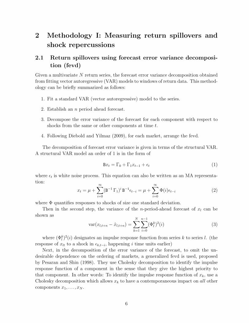
2 Methodology I: Measuring return spillovers and

shock repercussions

2.1 Return spillovers using forecast error variance decomposi-

tion (fevd)

Given a multivariate N return series, the forecast error variance decomposition obtained

from fitting vector autoregressive (VAR) models to windows of return data. This method-

ology can be briefly summarized as follows:

1. Fit a standard VAR (vector autoregressive) model to the series.

2. Establish an n period ahead forecast.

3. Decompose the error variance of the forecast for each component with respect to

shocks from the same or other components at time t.

4. Following Diebold and Yilmaz (2009), for each market, arrange the fevd.

The decomposition of forecast error variance is given in terms of the structural VAR.

A structural VAR model an order of 1 is in the form of

Bxt = Γ0 + Γ1xt−1 + εt (1)

where εt is white noise process. This equation can also be written as an MA representa-

tion:

xt = µ+∞∑i=0

(B−1 Γ1)i B−1εt−i = µ+

∞∑i=0

Φ(i)εt−i (2)

where Φ quantifies responses to shocks of size one standard deviation.

Then in the second step, the variance of the n-period-ahead forecast of xl can be

shown as

var(xl,t+n − xl,t+n) =N∑k=1

n−1∑i=0

(Φkl )

2(i) (3)

where (Φkl )

2(i) designates an impulse response function from series k to series l. (the

response of xlt to a shock in εk,t−i, happening i time units earlier)

Next, in the decomposition of the error variance of the forecast, to omit the un-

desirable dependence on the ordering of markets, a generalized fevd is used, proposed

by Pesaran and Shin (1998). They use Cholesky decomposition to identify the impulse

response function of a component in the sense that they give the highest priority to

that component. In other words: To identify the impulse response function of xk, use a

Cholesky decomposition which allows xk to have a contemporaneous impact on all other

components x1, . . . , xN .

6

The fevd is then expressed in terms of the ratios∑n−1i=0 (Φk

l )2(i)∑N

k=1

∑n−1i=0 (Φk

l )2(i)

, l = 1, . . . , N. (4)

The fevd gives the share of forecast variability in xl due to shocks in xk, or, in other

words, the return spillovers to volatility since return series is used in the model. After

obtaining the fevd for each market, all spillovers can be arranged in the so-called spillover

matrix as follows where N=4:

from return (xk)

x1 x2 x3 x4x1 � � � �

to forecast error variability share in (xl) x2 � � � �x3 � � � �x4 � � � �

(5)

Each row thus sums up to 1 (or 100%) and provides a breakdown of the forecast

error variance of the corresponding stock index return with respect to shock origins in

terms of percentages. Each entry in the spillover table is called a directional spillover.

Schematically, Diebold and Yilmaz (2009) introduced the spillover index,∑�∑

� +∑

�. (6)

The network structure of the spillover matrix with respect to the propagation of

shocks is a broad perspective, using the concepts from population, Markov Chain theory

and information theory. The methodology developed by Diebold and Yilmaz (2009) is

used in this paper to extent the spillover idea (Schmidbauer et al. (2012)) and to find

supplementary measures of market connectedness. More information about the spillover

methodology can be found in Diebold and Yilmaz (2009).

2.2 Shock repercussions and Entropy

The starting point for shock repercussions is the spillover matrix on a given period. As

it is described in the previous section row entries characterize the markets’ exposition

to shocks while the propagation of the shock needs to be read column-wise. Due to

the network structure of the spillover matrix, the population and Markov chain theory

is used by Schmidbauer et al. (2012) to answer the following question: How are future

volatilities across markets affected by a hypothetical shock hitting xk on day t? How

can we measure the strength of market repercussions of a shock?

Let Mt denote the spillover matrix for day t. The propagation of the shock across

the markets within day t can take place in a short time interval of unspecified length.

The shock propagation (repercussion of the shock) can be modeled as

ns+1 = Mt · ns, s = 0, 1, 2, . . . , (7)

7

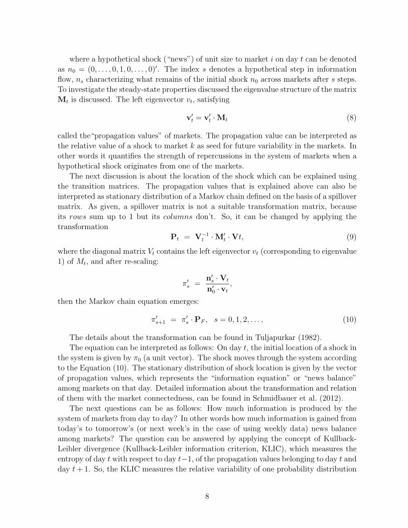
where a hypothetical shock (“news”) of unit size to market i on day t can be denoted

as n0 = (0, . . . , 0, 1, 0, . . . , 0)′. The index s denotes a hypothetical step in information

flow, ns characterizing what remains of the initial shock n0 across markets after s steps.

To investigate the steady-state properties discussed the eigenvalue structure of the matrix

Mt is discussed. The left eigenvector vt, satisfying

v′t = v′t · Mt (8)

called the“propagation values” of markets. The propagation value can be interpreted as

the relative value of a shock to market k as seed for future variability in the markets. In

other words it quantifies the strength of repercussions in the system of markets when a

hypothetical shock originates from one of the markets.

The next discussion is about the location of the shock which can be explained using

the transition matrices. The propagation values that is explained above can also be

interpreted as stationary distribution of a Markov chain defined on the basis of a spillover

matrix. As given, a spillover matrix is not a suitable transformation matrix, because

its rows sum up to 1 but its columns don’t. So, it can be changed by applying the

transformation

Pt = V−1t · M′t · Vt, (9)

where the diagonal matrix Vt contains the left eigenvector vt (corresponding to eigenvalue

1) of Mt, and after re-scaling:

π′s =n′s · Vt

n′0 · vt,

then the Markov chain equation emerges:

π′s+1 = π′s · PF , s = 0, 1, 2, . . . , (10)

The details about the transformation can be found in Tuljapurkar (1982).

The equation can be interpreted as follows: On day t, the initial location of a shock in

the system is given by π0 (a unit vector). The shock moves through the system according

to the Equation (10). The stationary distribution of shock location is given by the vector

of propagation values, which represents the “information equation” or “news balance”

among markets on that day. Detailed information about the transformation and relation

of them with the market connectedness, can be found in Schmidbauer et al. (2012).

The next questions can be as follows: How much information is produced by the

system of markets from day to day? In other words how much information is gained from

today’s to tomorrow’s (or next week’s in the case of using weekly data) news balance

among markets? The question can be answered by applying the concept of Kullback-

Leibler divergence (Kullback-Leibler information criterion, KLIC), which measures the

entropy of day t with respect to day t−1, of the propagation values belonging to day t and

day t+ 1. So, the KLIC measures the relative variability of one probability distribution

8

πa with respect to the variability of a second distribution πb:

KLIC =∑i

πa(i) · log2

(πa(i)

πb(i)

); (11)

In the concept of market connectedness, KLIC measures the initial information con-

tent of a shock (news) with respect to the news balance between markets in the long

run. In cases where πb characterizes the system of markets, KLIC is called the “relative

market entropy”.

As it is explained at the beginning of this section, a hypothetical shock to a market

will change the equilibrium, but then the market will “digest” the shock and reach the

equilibrium again. How fast can the market converge back to the equilibrium after

being hit by a shock? An appropriate measure for the speed of convergence is the

Kolmogorov-Sinai (KS) entropy. Demetrius (1974) introduced this entropy measure to

population theory as“population entropy”; Tuljapurkar (1982) relates it to the rate of

convergence of a population. The rate of convergence to equilibrium defined as

KS = −∑i,j

π(i) · log2

(p

pijij

). (12)

where pij denotes the entries in the transition matrix of the Markov chain as in the

Equation (10) and π(i) are the stationary probabilities. Schmidbauer et al. (2012) ex-

amine the concept developed by Tuljapurkar (1982) and adjust the definition in terms

of market connectedness.

3 Methodology II: Measuring volatility spillovers and

shock repercussions

3.1 Volatility spillovers

Spillovers are important to understand the financial market interdependence. The spillover

intensity is time-varying and this time-variation is fairly different for returns vs. volatil-

ities.

The same fevd methodology is used, as it is in the Section 2, to obtain the volatility

spillovers. The xt in the Equation (2) that we meant return is now means volatility. So,

we forecast the volatilities instead of returns. As in the return spillovers, where we need

weekly return series, in this case we need weekly return volatility series to apply the

VAR methodology for producing volatility spillovers. The methodology to obtain the

return volatility series using the German and Klass’ formula and the intuition behind it

is explained in Section 3.1.1 and the method of applying the formula to our data will be

explained in Section 4.

9

3.1.1 Obtaining Daily Return Volatilities

There are different estimation methods to obtain the stock return volatility. Our ini-

tial point will be the estimation method of German and Klass (1980) and we discuss

the intuition behind it. We answer the question that why we can use the estimation

method of German and Klass (1980) instead of a GARCH methodology or can we mod-

ify the formula in a different way to estimate the volatility series. As, we can see from

the Equation 15, the major difference of the two methodologies are, the German and

Klass methodology uses only today’s information while GARCH uses also the previous

information of the stock prices. The methodology of German and Klass (1980) uses the

historical opening, closing, high and low prices to estimate the volatility series. The

model assumes that security prices are governed by a diffusion process of the form,

P (t) = φ(B(t)) (13)

where P is the price, t is time and φ is a monotonic time independent transformation

where we can obtain the maximum and minimum values of B and P . B(t) is a diffusion

process with the differential representation

dB = σdz (14)

where dz is a standard Gauss-Wiener process and σ is an unknown constant to be

estimated.

The methodology of German and Klass (1980) covers the usual hypothesis of the

geometric Brownian motion of stock prices to estimate the return volatilities of the

series. Although, the starting point of the estimation method is the Brownian motion,

they mention some limitations of this methodology. They did modifications on the

estimation method and use three different estimation methodology. The first one, uses

only the opening and closing prices of the stock market data and the other two uses high

and low prices in addition to the opening and closing prices. Using also high and low

prices in the estimation model, gives us more information about the data, since high and

low prices during the trading interval express a continuous information about the prices

changes while opening and closing prices are only ‘snapshots’ of the process. Finally,

they found the formula below, which have the best efficiency factor among the three

methodologies.

σ2t = 0.511(Ht − Lt)

2 − 0.019[(Ct −Ot)(Ht + Lt − 2Ot) − 2(Ht −Ot)(Lt −Ot)]

− 0.383(Ct −Ot)2,

(15)

where Ot (Ht, Ct, Lt) is the natural logarithm of the opening price in day i (daily high,

Friday closing, daily low) in day t. The methodology of how we implement this formula

to obtain the weekly prices, not the daily ones, is explained in Section 4. For simplicity,

we call the stock return volatility series as “volatility series” throughout the paper.

10

Explaining the coefficients of the Formula (15) is beyond the scope of this project for

now. Instead of asking; “where does the coefficients come from?”, we want to show the

intuition behind the formula. We develop a strategy to understand the methodology and

the intuition. We use the same approach like in the German and Klass methodology and

simulate a Brownian bridge to understand the intuition behind this estimation method.

Brownian Bridge is formulated as follows;

Xt = Btµ,σ − tB1

µ,σ (16)

where Bt is a Brownian motion with µ and dispersion σ, and 0 ≤ t ≤ 1.

Obviously, X0 and X1 are 0. So, we know the starting and ending points. In contrast

to the Brownian motion, we know the ending point of the process which is the closing

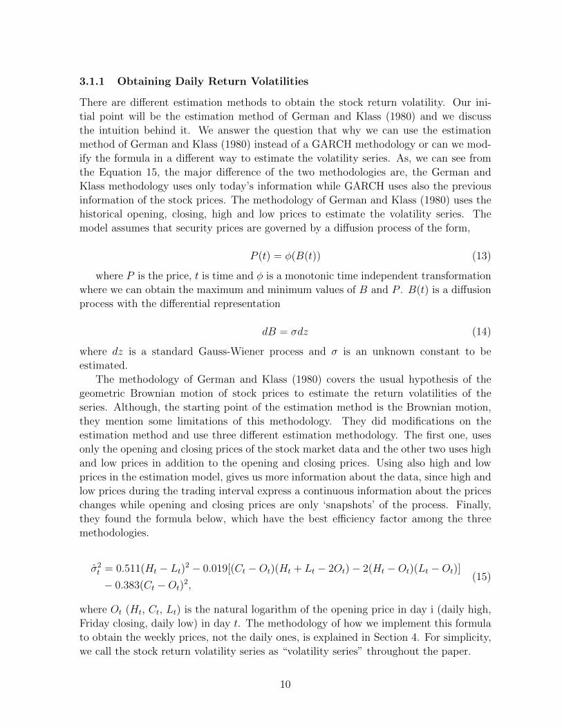
price in our case. The idea behind simulating Brownian Bridges is that, if we can find

a relation between the sigma and the maximum and minimum values of the trading

day then we can estimate the sigma, since we have the information about the high and

low stock prices during the trading day. So, we try to answer the question; Can we

find a relation among the maximum and minimum values and the σ value? In other

words, is it possible to estimate the σ, using the maximum and minimum value of

the stock price. First, we simulate Brownian Bridge where Bts are normally randomized

numbers. We simulate Brownian Bridges using different normally randomized Bts. Then,

we simulate the Brownian Bridge simulations for different σ values. We have Brownian

Bridge simulations with different normalized random Brownian motions. So, now we can

obtain the maximum and minimum values of the Brownian Bridges for every simulation.

Then, we plot the difference of ‘maximum-minimum’ values for different sigmas to see

that whether there is a relation among them. If we can find a relation, it means, we

can estimate a sigma value by using the difference of ‘maximum-minimum’ values of

a Brownian bridge. The graph of ‘maximum-minimum’ for different values of sigma is

expressed in Figure 1.

As we can see from the Figure 1, there is a linear relationship between the ‘maximum-

minimum’ value and the sigma. So, if we know the maximum and minimum value of the

Brownian Bridge (which in our case it will be the high and low prices of stock in day

i) then using this information we can estimate the sigma value. Since, only the slope

differ in the relation of ‘maximum-minimum’ values and sigma, then we can specify an

“average” slope to decide the relation and we can use this average slope to estimate the

sigma value. The histogram of the slope values is given in Figure 2.

As, we can see from the histogram the average of the slopes lies in the interval of

(6,7). Obviously, this is not the value we can see in the Formula (15), but, at least it

gives us an intuition of the methodology. We have not answered some questions, for

instance, what if we have a drift together with the diffusion. In our study we always

have a zero mean with different sigma values. So, the results will affect if we have a drift

term with the volatility. Second, we want to find a way to estimate the sigma when the

day is not finished due to an holiday or another reason. Now, to say something about

11

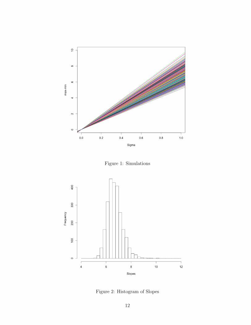
Figure 1: Simulations

Figure 2: Histogram of Slopes

12

the sigma our assumptions are made such that the day is complete and will finish at

time 1.

3.1.2 Garch Methodology

We will compare the different methodologies of estimating volatility series and discuss

the them to find the better estimation for our study. For the first step, we will compare

the German and Klass (1980) methodology explained in Section 3.1.1 and the Garch

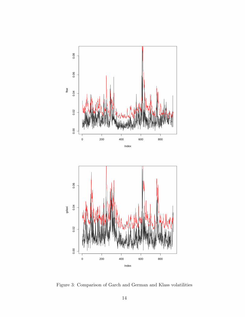
methodology As we have mentioned in the previous Section, the Garch methodology

uses today’s information as well as the previous day’s information of the stock prices.

Since, the methodology also affected by the previous days, as we expected we found

that the volatilities are generally higher than what we have found in the German and

Klass methodology. Dow Jones (USA) and Gdaxi (Germany) volatilities computed with

German and Klass, and Garch methodology are in Figure 3. To examine which estima-

tion methodology is better for the sake of our project, we will analyze the methodology

with the appropriate data in Section 5 and we compare the results with respect to the

different volatility series obtained by two methodologies.

3.2 Shock repercussions and entropy for volatility

The market entropy is a tool to measure the amount of information, created from week

to week. Comparing the return KLIC and volatility KLIC is very important to analyze

especially the intervals where the behaviour of the two are different. We will see in the

Empirical part (Section 5) in detailed that there are different spikes in different times

for return and volatility market entropies.

For the KS entropy, which is the speed of convergence back to the equilibrium after

a shock, it is shown that return and volatility entropies have different characteristics for

some intervals. Especially in the case of some specific events, the speed of information

digestion varies in the case of return and volatility KS entropies. On the other hand,

the KS entropy has another important characteristic. As it is discussed in Section 5, the

overall pattern of KS entropy and spillovers are similar for both return and volatilities.

The same Markov chain approach is used, as in the Section 2.2, to produce the KLIC

and KS entropy. The same methodology is used, which is developed by Schmidbauer

et al. (2012), using the weekly volatility series obtained from Equation (15) instead of

weekly return series.

13

0 200 400 600 800

0.00

0.02

0.04

0.06

0.08

Index

ftse

0 200 400 600 800

0.00

0.02

0.04

0.06

Index

gdax

i

Figure 3: Comparison of Garch and German and Klass volatilities

14

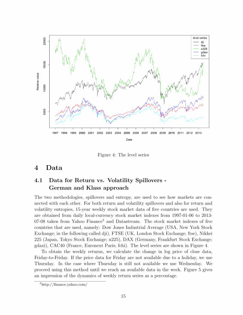
Figure 4: The level series

4 Data

4.1 Data for Return vs. Volatility Spillovers -

German and Klass approach

The two methodologies, spillovers and entropy, are used to see how markets are con-

nected with each other. For both return and volatility spillovers and also for return and

volatility entropies, 15-year weekly stock market data of five countries are used. They

are obtained from daily local-currency stock market indexes from 1997-01-06 to 2013-

07-08 taken from Yahoo Finance5 and Datastream. The stock market indexes of five

countries that are used, namely: Dow Jones Industrial Average (USA, New York Stock

Exchange; in the following called dji), FTSE (UK, London Stock Exchange; ftse), Nikkei

225 (Japan, Tokyo Stock Exchange; n225), DAX (Germany, Frankfurt Stock Exchange;

gdaxi), CAC40 (France, Euronext Paris; fchi). The level series are shown in Figure 4.

To obtain the weekly returns, we calculate the change in log price of close data,

Friday-to-Friday. If the price data for Friday are not available due to a holiday, we use

Thursday. In the case where Thursday is still not available we use Wednesday. We

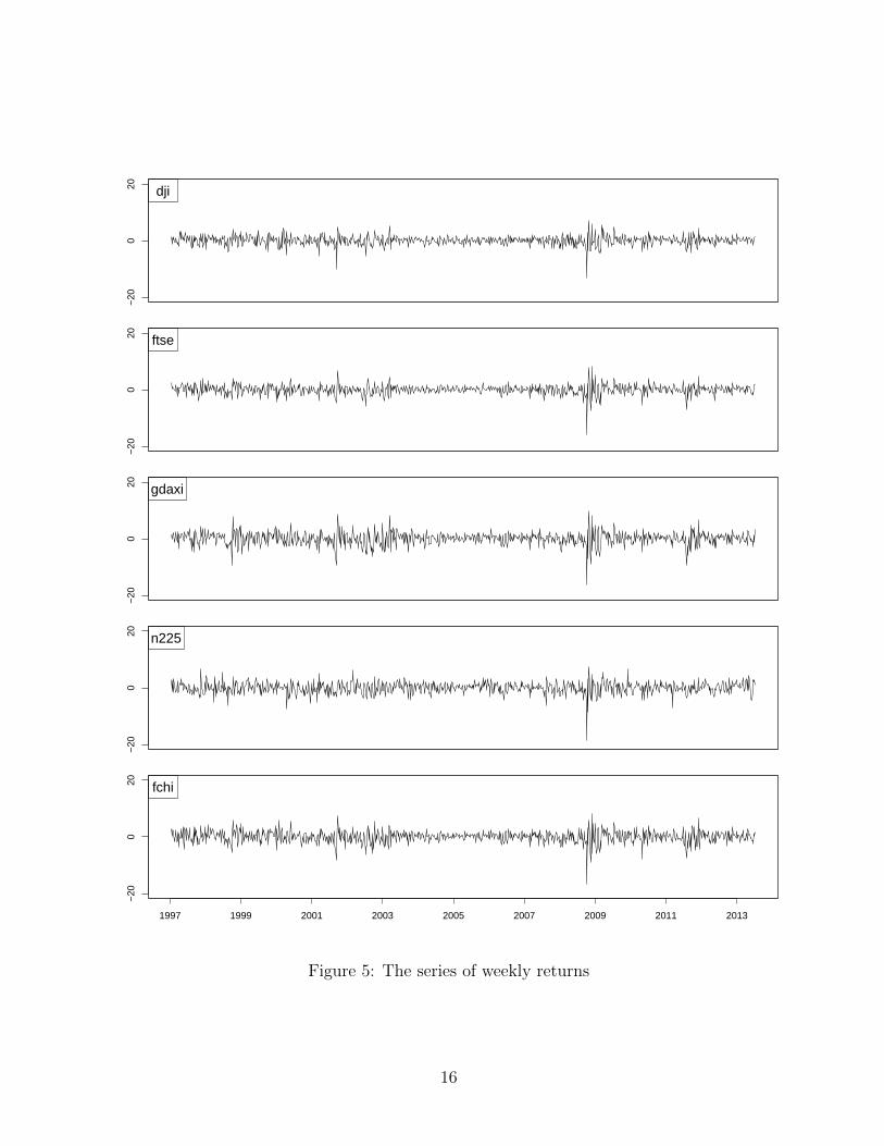
proceed using this method until we reach an available data in the week. Figure 5 gives

an impression of the dynamics of weekly return series as a percentage.

5http://finance.yahoo.com/

15

−20

020 dji

−20

020 ftse

−20

020 gdaxi

−20

020 n225

1997 1999 2001 2003 2005 2007 2009 2011 2013

−20

020 fchi

Figure 5: The series of weekly returns

16

The formula, developed by Diebold and Yilmaz (2009), that is explained in the

Section 3 is used to estimate the weekly volatilities. Following German and Klass (1980)

and Alizadeh et al. (2002), the underlying daily high/low/open/close data is used to

obtain weekly high, low, opening and closing prices to use the values in formula (15).

For the weekly closing price the same method is used as in return: If available, Friday

is used as weekly closing price, otherwise the previous available day is used. If available

Monday is used as a weekly opening price, otherwise the next available day of the week

is used. The highest value from Monday to Friday is used as weekly high price and

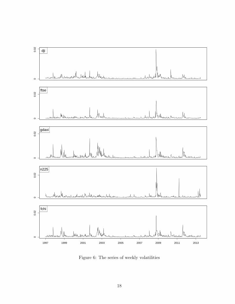
the lowest value from Monday to Friday is used as weekly low price. Figure 6 gives an

impression of the development of weekly volatilities.

4.2 Data for Return vs. Volatility Spillovers -

using GARCH approach

The second empirical part consists of daily closing quotations of the Russian stock in-

dex (rts) and the five stock indices representing stock markets in the ”Systemic Five”

countries: Dow Jones Industrial Average (USA; dji), FTSE (UK;ftse), Euro Stoxx 50

(euro area; sx5e), Nikkei 225 (Japan; n225), and SSE Composite (China; spec). The

time period begins with 1997-07-03 (the first day for which all six series were available)

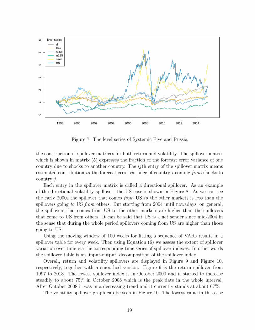
and ends 2015-05-22. So, we have 4660 observations on total. The level series are shown

in Figure 7. We will use the weekly return series with the same methodology used in

Session 4.1 and for the volatility estimation we will use GARCH methodology instead

of using the German and Klass approach and we will compare the two computing the

volatility spillovers. We will also compare the return and volatility spillovers of the data

as in Session 4.1.

5 Empirical findings

With the stock market data explained in Section 4.1 Section 4.2, market connectedness

can now be obtained by applying methodologies I and II (Section 2 and Section 3) using

weekly returns and weekly volatilities with the German and Klass methodology and daily

return and daily volatility with the GARCH methodology.

5.1 Directional and overall spillovers -

Example 1: German and Klass methodology

In this section, we provide an analysis of five countries’ stock market weekly sequences

of return and volatility spillovers (which means, weekly time series of spillover index

values). First, we obtain the spillover matrices which resulted from fitting a sequence of

VAR models along the steps outlined in Section 2 for return spillovers and Section 3 for

volatility spillovers. Moving windows of 100 weeks and 5-week-ahead forecast are used in

17

00.

025

dji

00.

02

ftse

00.

02

gdaxi

00.

02

n225

1997 1999 2001 2003 2005 2007 2009 2011 2013

00.

02

fchi

Figure 6: The series of weekly volatilities

18

01

23

45

6 level series

djiftsesx5en225ssecrts

1998 2000 2002 2004 2006 2008 2010 2012 2014

Figure 7: The level series of Systemic Five and Russia

the construction of spillover matrices for both return and volatility. The spillover matrix

which is shown in matrix (5) expresses the fraction of the forecast error variance of one

country due to shocks to another country. The ijth entry of the spillover matrix means

estimated contribution to the forecast error variance of country i coming from shocks to

country j.

Each entry in the spillover matrix is called a directional spillover. As an example

of the directional volatility spillover, the US case is shown in Figure 8. As we can see

the early 2000s the spillover that comes from US to the other markets is less than the

spillovers going to US from others. But starting from 2004 until nowadays, on general,

the spillovers that comes from US to the other markets are higher than the spillovers

that come to US from others. It can be said that US is a net sender since mid-2004 in

the sense that during the whole period spillovers coming from US are higher than those

going to US.

Using the moving window of 100 weeks for fitting a sequence of VARs results in a

spillover table for every week. Then using Equation (6) we assess the extent of spillover

variation over time via the corresponding time series of spillover indexes. In other words

the spillover table is an ‘input-output’ decomposition of the spillover index.

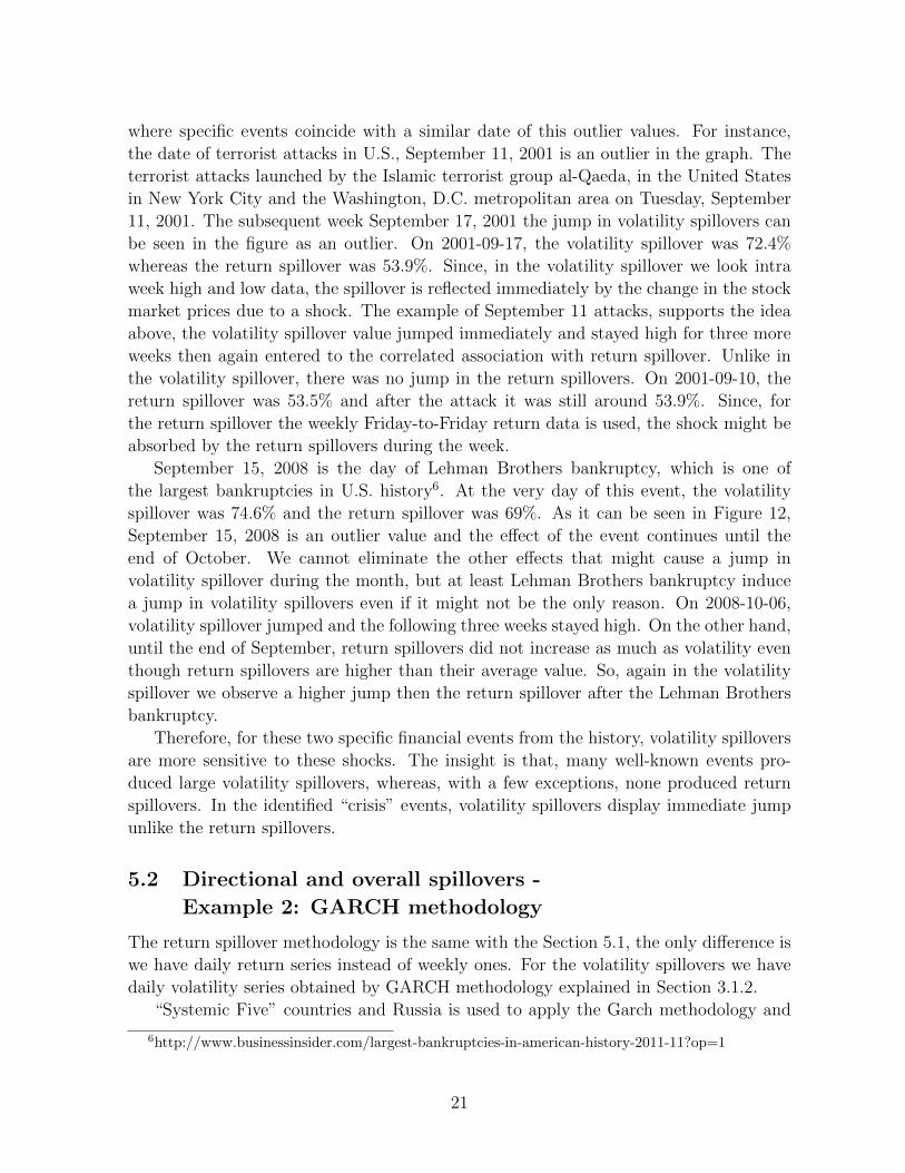
Overall, return and volatility spillovers are displayed in Figure 9 and Figure 10,

respectively, together with a smoothed version. Figure 9 is the return spillover from

1997 to 2013. The lowest spillover index is in October 2000 and it started to increase

steadily to about 75% in October 2008 which is the peak date in the whole interval.

After October 2008 it was in a decreasing trend and it currently stands at about 67%.

The volatility spillover graph can be seen in Figure 10. The lowest value in this case

19

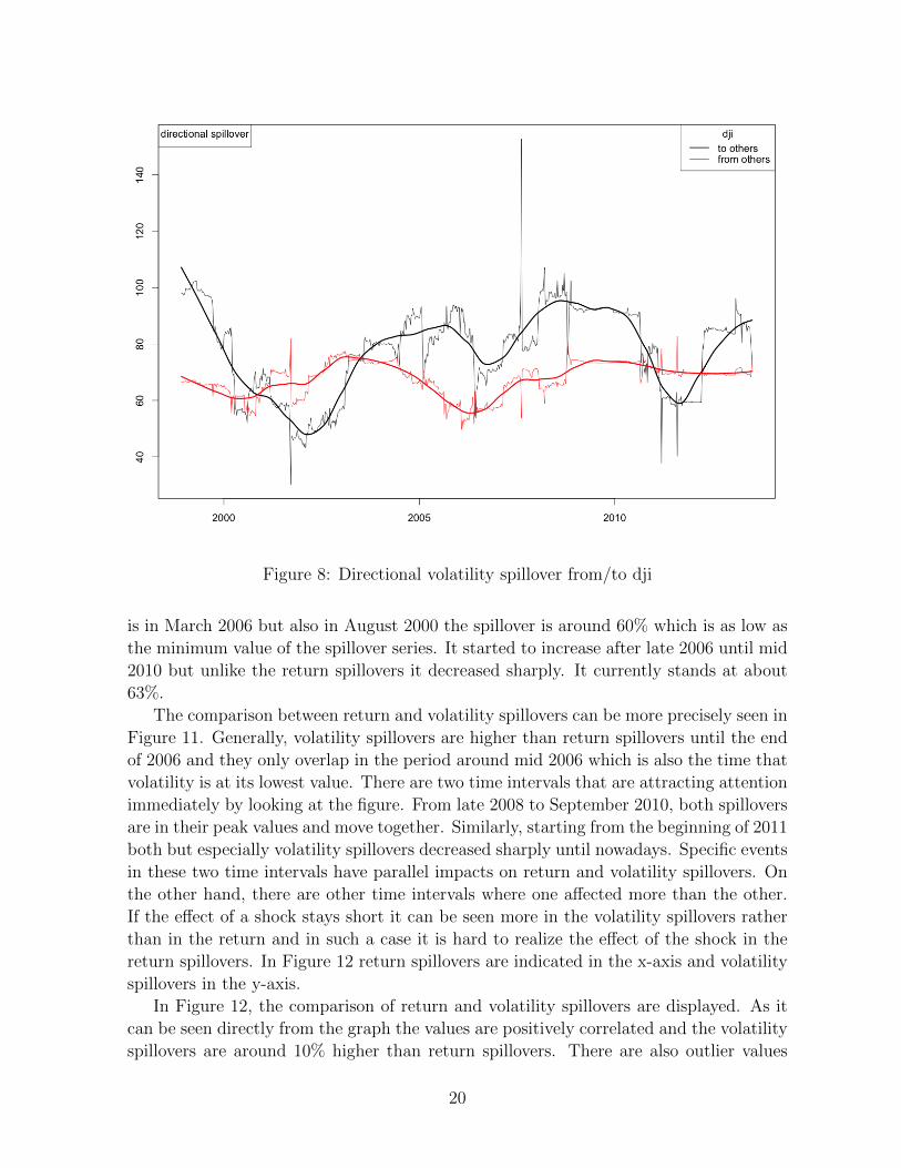
Figure 8: Directional volatility spillover from/to dji

is in March 2006 but also in August 2000 the spillover is around 60% which is as low as

the minimum value of the spillover series. It started to increase after late 2006 until mid

2010 but unlike the return spillovers it decreased sharply. It currently stands at about

63%.

The comparison between return and volatility spillovers can be more precisely seen in

Figure 11. Generally, volatility spillovers are higher than return spillovers until the end

of 2006 and they only overlap in the period around mid 2006 which is also the time that

volatility is at its lowest value. There are two time intervals that are attracting attention

immediately by looking at the figure. From late 2008 to September 2010, both spillovers

are in their peak values and move together. Similarly, starting from the beginning of 2011

both but especially volatility spillovers decreased sharply until nowadays. Specific events

in these two time intervals have parallel impacts on return and volatility spillovers. On

the other hand, there are other time intervals where one affected more than the other.

If the effect of a shock stays short it can be seen more in the volatility spillovers rather

than in the return and in such a case it is hard to realize the effect of the shock in the

return spillovers. In Figure 12 return spillovers are indicated in the x-axis and volatility

spillovers in the y-axis.

In Figure 12, the comparison of return and volatility spillovers are displayed. As it

can be seen directly from the graph the values are positively correlated and the volatility

spillovers are around 10% higher than return spillovers. There are also outlier values

20

where specific events coincide with a similar date of this outlier values. For instance,

the date of terrorist attacks in U.S., September 11, 2001 is an outlier in the graph. The

terrorist attacks launched by the Islamic terrorist group al-Qaeda, in the United States

in New York City and the Washington, D.C. metropolitan area on Tuesday, September

11, 2001. The subsequent week September 17, 2001 the jump in volatility spillovers can

be seen in the figure as an outlier. On 2001-09-17, the volatility spillover was 72.4%

whereas the return spillover was 53.9%. Since, in the volatility spillover we look intra

week high and low data, the spillover is reflected immediately by the change in the stock

market prices due to a shock. The example of September 11 attacks, supports the idea

above, the volatility spillover value jumped immediately and stayed high for three more

weeks then again entered to the correlated association with return spillover. Unlike in

the volatility spillover, there was no jump in the return spillovers. On 2001-09-10, the

return spillover was 53.5% and after the attack it was still around 53.9%. Since, for

the return spillover the weekly Friday-to-Friday return data is used, the shock might be

absorbed by the return spillovers during the week.

September 15, 2008 is the day of Lehman Brothers bankruptcy, which is one of

the largest bankruptcies in U.S. history6. At the very day of this event, the volatility

spillover was 74.6% and the return spillover was 69%. As it can be seen in Figure 12,

September 15, 2008 is an outlier value and the effect of the event continues until the

end of October. We cannot eliminate the other effects that might cause a jump in

volatility spillover during the month, but at least Lehman Brothers bankruptcy induce

a jump in volatility spillovers even if it might not be the only reason. On 2008-10-06,

volatility spillover jumped and the following three weeks stayed high. On the other hand,

until the end of September, return spillovers did not increase as much as volatility even

though return spillovers are higher than their average value. So, again in the volatility

spillover we observe a higher jump then the return spillover after the Lehman Brothers

bankruptcy.

Therefore, for these two specific financial events from the history, volatility spillovers

are more sensitive to these shocks. The insight is that, many well-known events pro-

duced large volatility spillovers, whereas, with a few exceptions, none produced return

spillovers. In the identified “crisis” events, volatility spillovers display immediate jump

unlike the return spillovers.

5.2 Directional and overall spillovers -

Example 2: GARCH methodology

The return spillover methodology is the same with the Section 5.1, the only difference is

we have daily return series instead of weekly ones. For the volatility spillovers we have

daily volatility series obtained by GARCH methodology explained in Section 3.1.2.

“Systemic Five” countries and Russia is used to apply the Garch methodology and

6http://www.businessinsider.com/largest-bankruptcies-in-american-history-2011-11?op=1

21

Figure 9: Return Spillover

we will focus on the results and graphs of rts as an example. The daily series of direct

return spillovers from rts to others and from others to arts are displayed in Figure 13.

We can say from the figure that spillovers to rts have always been higher than spillovers

from rts. Return spillovers to rts rose sharply on 2014-12-17 the day after the Bank of

Russia announced an increase of its key interest rate, the Russian weekly repo rate, from

10.5 to 17 percent as an emergency move to retain the collapse of the rule’s value. The

big gap in from/to return spillovers lasted for about four months.

Then, we calculated the directional spillovers as we have done for example 1, for both

return and volatility spillovers. More specifically, with the daily volatility series that we

have obtained from the GARCH methodology, we calculated the volatility spillovers and

same methodology as example 1 is used but with daily returns instead of weekly ones,

we calculate the return spillovers for stock markets of six countries. Figure 14 displays

the directional volatility spillover for the case of Russia. The volatility spillover that

comes from Russia to others is less than the spillovers going to Russia from others until

the mid 2008. But stating from 2009 the spillovers to Russia from others increased a bit

and the effect from Russia to others became smaller. So, we can say that starting from

the second half of the period, Russia is a net sender in the sense that during the period

spillovers coming from Russia are higher than those going to Russia. But nowadays the

spillovers from others to Russia is started to increase again and the net sender situation

of Russia started to change.

22

Figure 10: Volatility Spillover

The volatility spillover obtained by the GARCH methodology can be seen in Figure

(15). The volatility spillover is always in an increasing trend but its peak value was at

the beginning of 2007. It is started to decrease starting from 2012 and it continue to

decrease. It currently stands at about 35%. Generally, volatility and return spillovers are

positively correlated with each other but volatility spillovers are higher than the return

ones around 10%. The reasons for this difference will be examined in the later versions

of this paper.

Propagation values quantify the relative importance of a market to act as a shock

propagator. In other words, the propagation value measure the network repercussions

of shocks. The propagation values of rts are displayed in Figure 16. The values were

gradually increasing since 1997, peaking in early 2012, and have begun to decrease

since then especially after 2014-12-17. When we compare the return spillovers and the

propagation values especially after December 2014, we can conclude that direct spillovers

tended to become more important, while network repercussions of shocks of rts decreased

in importance.

5.3 KLIC and KS entropy

- Relative market entropy (KLIC):

The information that is produced by the system of markets from week to week is

23

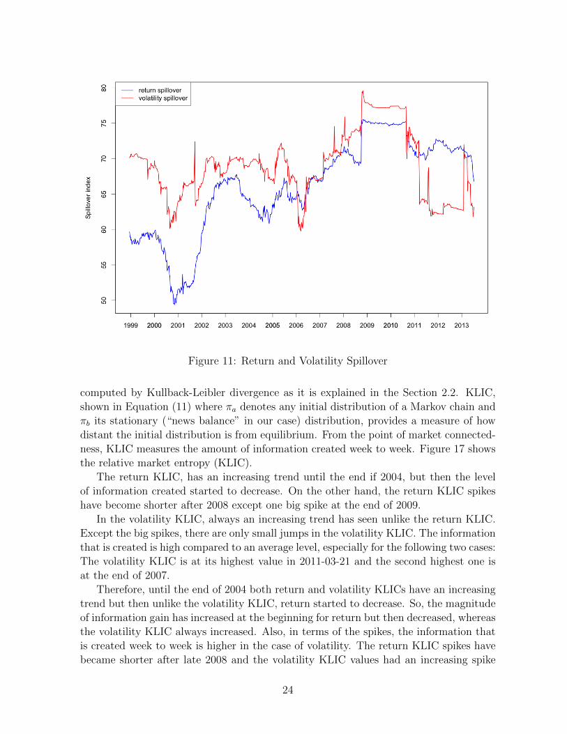
Figure 11: Return and Volatility Spillover

computed by Kullback-Leibler divergence as it is explained in the Section 2.2. KLIC,

shown in Equation (11) where πa denotes any initial distribution of a Markov chain and

πb its stationary (“news balance” in our case) distribution, provides a measure of how

distant the initial distribution is from equilibrium. From the point of market connected-

ness, KLIC measures the amount of information created week to week. Figure 17 shows

the relative market entropy (KLIC).

The return KLIC, has an increasing trend until the end if 2004, but then the level

of information created started to decrease. On the other hand, the return KLIC spikes

have become shorter after 2008 except one big spike at the end of 2009.

In the volatility KLIC, always an increasing trend has seen unlike the return KLIC.

Except the big spikes, there are only small jumps in the volatility KLIC. The information

that is created is high compared to an average level, especially for the following two cases:

The volatility KLIC is at its highest value in 2011-03-21 and the second highest one is

at the end of 2007.

Therefore, until the end of 2004 both return and volatility KLICs have an increasing

trend but then unlike the volatility KLIC, return started to decrease. So, the magnitude

of information gain has increased at the beginning for return but then decreased, whereas

the volatility KLIC always increased. Also, in terms of the spikes, the information that

is created week to week is higher in the case of volatility. The return KLIC spikes have

became shorter after late 2008 and the volatility KLIC values had an increasing spike

24

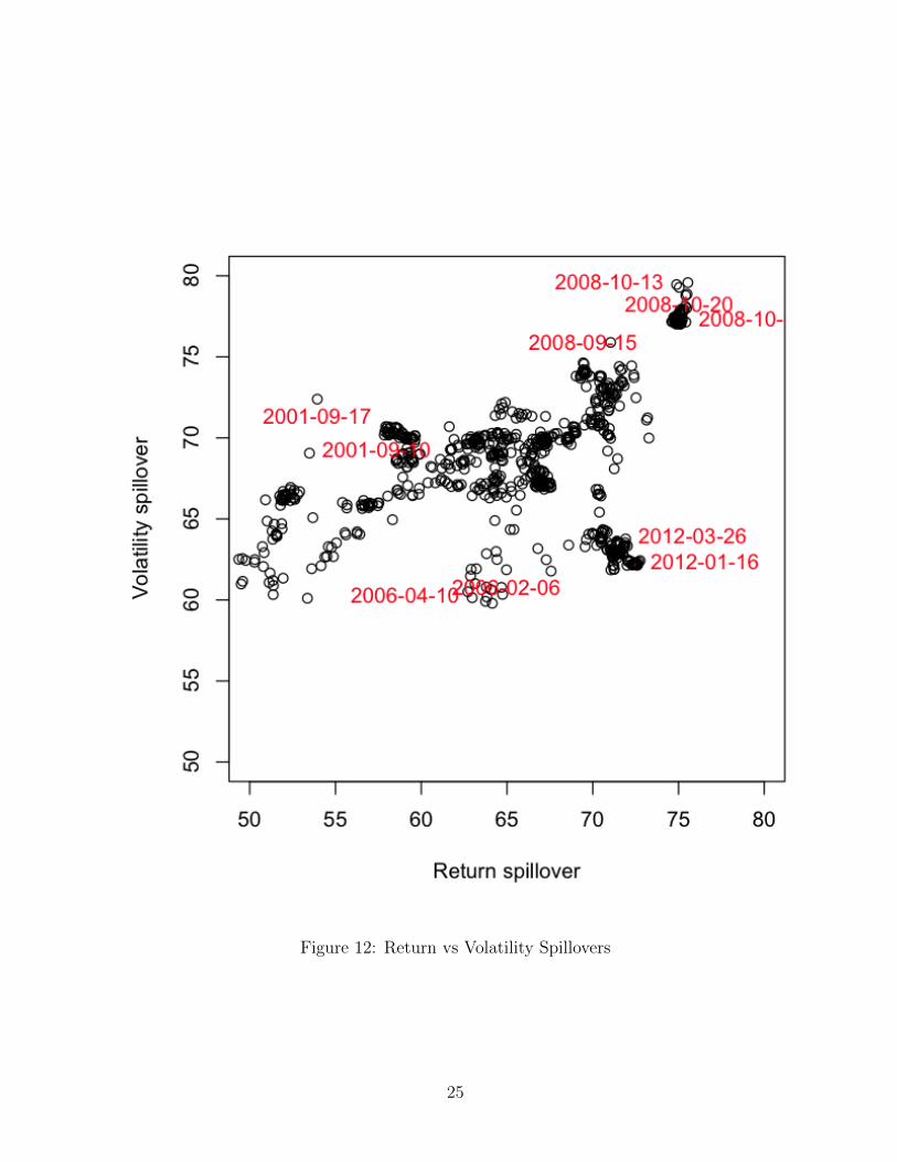
Figure 12: Return vs Volatility Spillovers

25

020

4060

80

1998 2000 2002 2004 2006 2008 2010 2012 2014

from rtsto rts

Figure 13: Direct Return Spillovers from and to arts

Figure 14: Directional Volatility Spillover from/to rts

26

Figure 15: Volatility Spillover with GARCH methodology

0.00

0.25

0.50

0.75

1.00

1998 2000 2002 2004 2006 2008 2010 2012 2014

rtsssecn225sx5eftsedji

Figure 16: Propagation Value of rts

27

Figure 17: Return and volatility relative market entropy

path, but the last spike was on March, 2011. The magnitude of the information created

is huge for volatility but not for the return.

Until now, we have discussed about example 1 explained in Section 5.1. Using the

second example, which we have explained the details in Section 5.2, relative market

entropy of volatility is shown in Figure 18. We can see big spikes especially mid 2010

and at the end of 2014. As we have examined in the spillover part, 2014-12-17 is the

day where the interest rates of Russian bank was in a sharp increasing trend and we

also observe the effect of this day in our KLIC results which was similar to the spillover

results. The magnitude of the information gain increase immediately after the day and

a few days later it disappears.

Figure 19 shows the relation of return and volatility relative market entropy values of

example 1. There is a linear association between return and volatility KLIC values. The

28

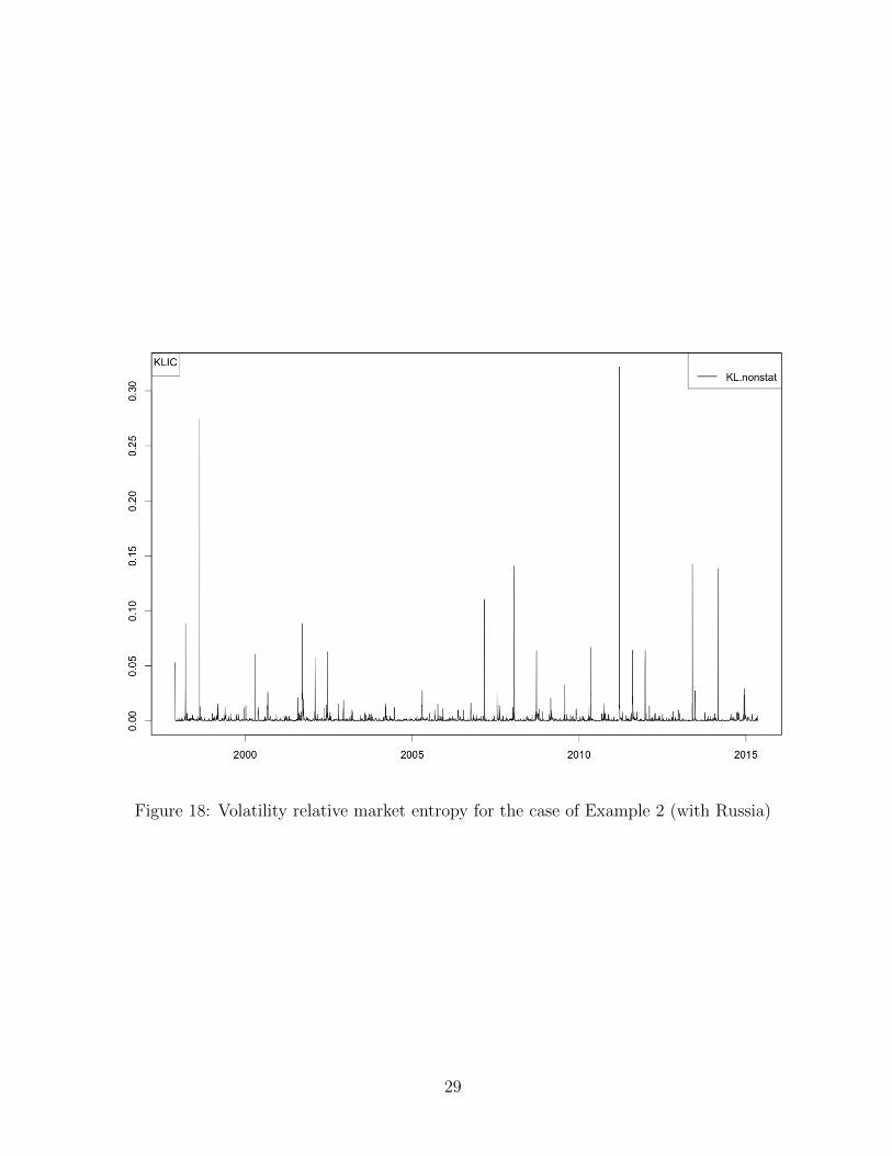
Figure 18: Volatility relative market entropy for the case of Example 2 (with Russia)

29

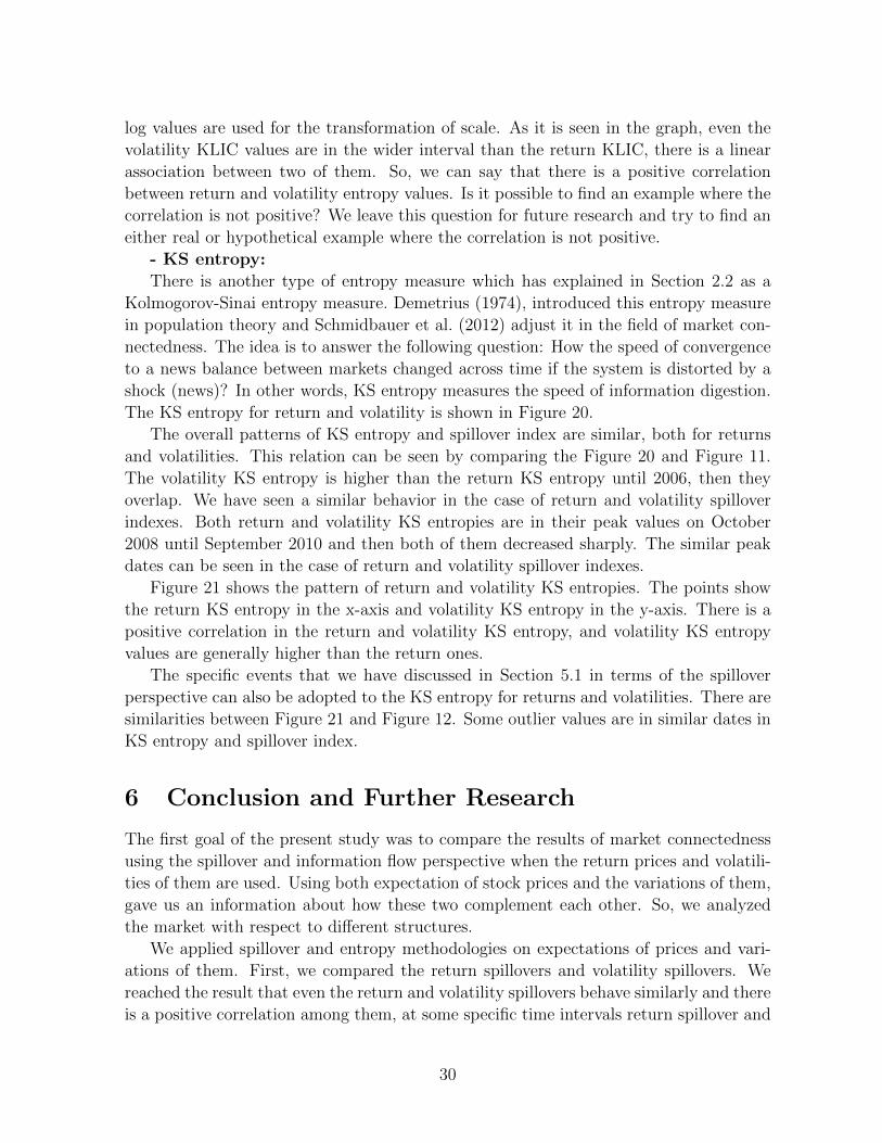
log values are used for the transformation of scale. As it is seen in the graph, even the

volatility KLIC values are in the wider interval than the return KLIC, there is a linear

association between two of them. So, we can say that there is a positive correlation

between return and volatility entropy values. Is it possible to find an example where the

correlation is not positive? We leave this question for future research and try to find an

either real or hypothetical example where the correlation is not positive.

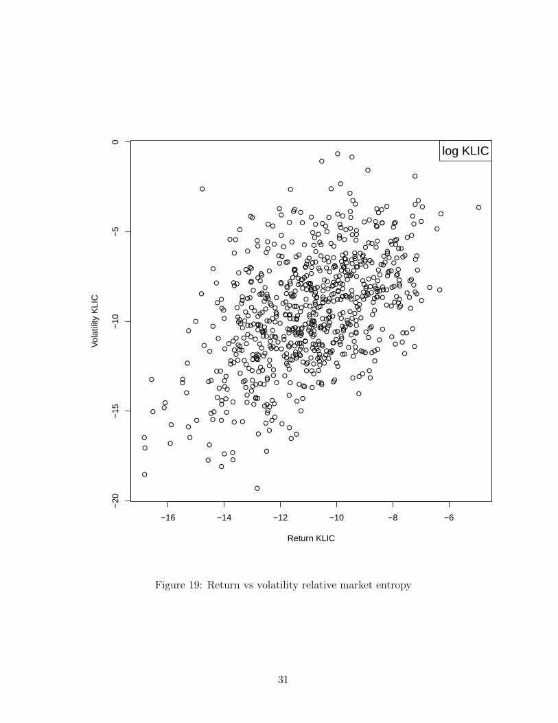
- KS entropy:

There is another type of entropy measure which has explained in Section 2.2 as a

Kolmogorov-Sinai entropy measure. Demetrius (1974), introduced this entropy measure

in population theory and Schmidbauer et al. (2012) adjust it in the field of market con-

nectedness. The idea is to answer the following question: How the speed of convergence

to a news balance between markets changed across time if the system is distorted by a

shock (news)? In other words, KS entropy measures the speed of information digestion.

The KS entropy for return and volatility is shown in Figure 20.

The overall patterns of KS entropy and spillover index are similar, both for returns

and volatilities. This relation can be seen by comparing the Figure 20 and Figure 11.

The volatility KS entropy is higher than the return KS entropy until 2006, then they

overlap. We have seen a similar behavior in the case of return and volatility spillover

indexes. Both return and volatility KS entropies are in their peak values on October

2008 until September 2010 and then both of them decreased sharply. The similar peak

dates can be seen in the case of return and volatility spillover indexes.

Figure 21 shows the pattern of return and volatility KS entropies. The points show

the return KS entropy in the x-axis and volatility KS entropy in the y-axis. There is a

positive correlation in the return and volatility KS entropy, and volatility KS entropy

values are generally higher than the return ones.

The specific events that we have discussed in Section 5.1 in terms of the spillover

perspective can also be adopted to the KS entropy for returns and volatilities. There are

similarities between Figure 21 and Figure 12. Some outlier values are in similar dates in

KS entropy and spillover index.

6 Conclusion and Further Research

The first goal of the present study was to compare the results of market connectedness

using the spillover and information flow perspective when the return prices and volatili-

ties of them are used. Using both expectation of stock prices and the variations of them,

gave us an information about how these two complement each other. So, we analyzed

the market with respect to different structures.

We applied spillover and entropy methodologies on expectations of prices and vari-

ations of them. First, we compared the return spillovers and volatility spillovers. We

reached the result that even the return and volatility spillovers behave similarly and there

is a positive correlation among them, at some specific time intervals return spillover and

30

●

●

●

●

●

●

●

● ●

●

●

●●

●●

●●

●

●●

●●

●

●

●●

●

● ●

●●●

●

●

●

●

●

●

●

●

●

●

●

●

●● ●●

●

●

●

●

●

●

●

●

●

●

●

●

●

●

●

●

●

●

●

●

●

●

●

●●●

●

●●

●

●

●

●

●●

●

●

●

●

●

●

●

●

●●

●

●

●

●

●●

●

●●

●

●

●●

●

●

●

●

●

●●

●

●

●

●

●

●

●

●

● ●

●

●

●

●

●

●●

●

●

●●

●

●

●

●

●

●

●

●

●

●

●

●

●●

●

●

●

●

●

●

●

●

●

●

●

●

●

●

●

●

●

●

●

●

●

●

●

●

●●

●●

●

●

●● ●

●

●

●

●

●

●●

●

●

●

●

●

●

●●

●

●

●

●

●

●

●

●

●

●

●

●

●

●

●

●

●

●

●

●

●

●●

●

●

●

●

●

●

●

●

●●

●●

●

●

●

●●

●

●

●

●

●

●

●

●

●

●

●

●

●

●

●

●

● ●

●

●

●

●

● ●

●

●

●

●

●

●

●

●

●●

● ●

●

●

●

●

●

●

●

●

●●

●●

●

●

●●

●

● ●

●

●

●

●

●

●●

●

●

●

●

●

●

●

●●

●

●

● ●

●

●

●

●

●

●●

●

●

●

●

●

●

●●

● ●●

●

●●

●●

●

●

●

●

●

●

●

●

●

●

●

●

●●

●

●

●

●

●●

●

●●

●

●

●

●

●

●

●

●

●

●

●

●●

●

●●

●

●

●

●

●

●●

●

●

●●

●

●

●

●

●

●

●

●

●

●

●

●

●●

●●

●

●

●

●

●

●

●

●

●●

●●

●

●

●

●

●

●

●

●

●

●

●

●

●

●

●

●

●

●

●

●

● ●

●

●

●

●

●

●

●

●

●

●

●

●

●

●●

●

●

●

●

●

●

●

●

●

●

●

●

●

●

● ●●

●

●

●

●

●

●

●

●

●

●

●

●

●

●

●

●

●

●

●

●

●

●

●

●

●

●

●

●

●

●

●

●

●

●

●

●

●

●

●

●

●

●

●

●●

●

●●

●

●

●

●

●

●

●

●

●

●

●

●

●

●

●

●

●

●

●●

●

●

●

●

●

●

●

●

●

●

●

●●

●

●

●

●

●

●

●

●

●

●

●

●

●

●

●

●

●

●

●

●

●

●

●●

●

●

●

●

●

●●●

●●

●

●●

●●

●

●

●

●

●

●

●

●

●

●●

●

●

●

●●●

●

●

●

●

●

●

●

●

●

●

●

●

●

●

●

●

●

●

●

●

●

●

●

●

●

●●

●

●

●

●●

●

●

●

●

●

●

●

●●

●

●●

●

●●

●

●

●

●

●

●

●

●

●

●

●●

●

●●

●

●

●

●

●

●

●

●

●

●

●

●

●

●

●●●

●

●

●

●●

●

●

●

●

● ●

●

●

●

●

●●

●

●

●●

●

●

●

●

●

●

●

●●

●

●●

●

●●

●

●

●

●

●

●

●

●●

●

●

●

●

●

●

●●

●

● ●

●●

●

●

●

●

●

●

●

●

●

●

●

●

●

●

●

●

●

●

●

●

●

−16 −14 −12 −10 −8 −6

−20

−15

−10

−5

0

Return KLIC

Vol

atili

ty K

LIC

log KLIC

Figure 19: Return vs volatility relative market entropy

31

Figure 20: Return and volatility KS entropy

volatility spillover act different. We explained these results in terms of a “crisis” or an

important event from the history.

The results obtained from KLIC and KS entropy showed us the information gain

comes from either using the return or volatility series. In the KLIC results, the amount

of information created week to week had different pattern in the case of return than the

volatility. The spikes from the volatility is higher than the spikes coming from return.

The magnitude of the information created has been increasing for volatility but in the

return there are time intervals where information created has been decreasing.

There is a positive correlation between the values of return market entropy and

volatility market entropy. In the further research of this study we will examine the

reason of this correlation and create an example where there is no correlation or the

correlation is negative. Therefore, we can compare the information created in these two

cases where there are positive and negative correlations.

In the case of KS entropy, the similar situation like in the spillover index have found.

There is a positive relation in the return and volatility KS entropies, but at some specific

time intervals the volatility KS entropy, which gives us an information about the shock

digestion, is higher than the return KS. We analyze the reasons of this change as we did

in the spillover index. We will improve the entropy idea in the future study of the thesis

and examine the results in terms of economics events.

In addition, since we have used the weekly return and weekly volatility series, we

32

●●●●

●

●● ●● ●●●● ●●●● ●●

●●●●● ●●●● ● ●●● ●●●● ●●●● ●●

● ●●

●

●

●●

●●

● ● ●●●●

●●●●

●●

●

●

●

●

●●●

●

●●

●●●

● ●●●●

●● ●

●

●

●

●●

●

●●

●

●●●

●●

●

●● ●●

●

●●

● ●●

●●●

●

●

●●

● ●

●

● ●

●

●●

●●●●● ●●●●● ●● ●●

●●●

●●●

●

●

●

●

●● ●●●

●●

●● ● ●

● ●

●●●

●●

●● ●

●

● ●●

●●

●●●● ●●●

●●●●●

●

●

●

●

●●●

●

●●

●

●●

●

●

●

●●

●

●●

● ●●●●●●●●

●

●●

●

●

●

●●●●●●●●●●● ●●●

●

●●●●●●●

●●●●● ●

●

●

●●

●●●●●●●●

●●●●●●

●●●●●

●●●●●●●

●●●●●●

●

●

●●

●●

●●

● ●●

●

●●●●● ●

●●

●

●●

●●● ● ●●

●●

●●●

●

●

●

● ●●●●

● ● ●

●●●●●

●●●●● ●

●●●●●●●

●

●●

●

●●

●

●●

●

●●●●●●

●●● ●●

●

●

●

●

●

●●

● ●●

●

●

●

●

●●

●

●

●●

●

●

●

●●

●● ●●● ●● ●●●●

●

●●●●●●●

●●●●●●●●●●●●

●●

●●●

●●●●●●●●●●

●●●●●●●●●●

●

●

●●●●●●●●●●● ●●

●

●●

●●● ● ●

●●

●●●●●●

●

●

●●●●●●●●

●●

●●●●●●●

●●●●●● ●●●

●●

●

●●●●●

●

●●●●●●●●●●●●●●●●●●●●●●●●●●●●●●●●●●●●●●●●●●●●●●●●●●●●●●●

●

●●●●●●●●●●●●●●●●●●●

●●●●●●●●●●●●●●●

●●

●●●

●

●

●

●

●●

●●●●●

●●

●●

●● ●●

●●

●

●

●●

●

●●●●●●●●●●●

●●●●● ●●●

●

●

●●●●

●●●●

●● ●●●●● ●●●●●●●●●●●●●●●●●

●●●●●●●●●●●●●●●●●

●●●●●●●●●●●●●●●●●●●●●●●●●●●●

●●

●●●●●●

●

●●●●●●

●●

●

●●

●

●●

1.9 2.0 2.1 2.2 2.3

1.9

2.0

2.1

2.2

2.3

Return KS

Vol

atili

ty K

S

KS Entropy

Figure 21: Return vs volatility KS entropy

33

needed to obtain the weekly return and volatilities using daily data. We followed the

methodology of German and Klass (1980) to construct the weekly volatility series and

tried to understand the intuition behind the method. So, both spillover and informa-

tion flow perspective depended on the weekly return and volatility series that we have

obtained using the methodology explained in the paper. We have also used the GARCH

methodology to obtain the volatility series and we compared the results with German

and Klass methodology. We have used a new stock market data group to examine the

different effects and compare the two methodologies to calculate the volatility spillovers.

In our further study, we will develop the idea and also investigate the best methodology

of volatility estimation for our study.

We would like to mention that the present paper have been submitted and accepted

for presentation at the Ecomod conference, in Boston, United States, in July 2015.

34

References

Acemoglu, D., Carvalho, V., Ozdaglar, A., and Tahbaz-Salehi, A. (2012): The network

origins of aggregate fluctuations. Econometrica, 80, 1977–2016.

Alizadeh, S., Brandt, M.W. and Diebold, F.X. (2002): Range-based estimation of

stochastic volatility models, Journal of Finance, 57 (3), 1047-92.

Balli, F., Hajhoj, H.R., Basher, S.A., and Ghassan, H.B. (2015): An analysis of returns

and volatility spillovers and their determinants in emerging Asian and Middle Eastern

countries. International Review of Economics and Finance 39, 311–325.

Baur, D. and Jung R.C. (2006). Return and volatility linkages between the US and the

German stock market. Journal of International Money and Finance, 25, 598–613.

Bekaert, G., M. Ehrmann, M. Fratzscher, and A.J. Mehl (2012): Global crises and equity

market contagion. Available at SSRN: http://ssrn.com/abstract=1856881.

Bekiros, S.D. (2014): Contagion, decoupling and the spillover effects of the US financial

crisis: Evidence from the BRIC markets. International Review of Financial Analysis

33, 58–69.

Bubak, V., Kocenda, E. and Zikes F. (2011). Volatility Transmission in Emerging Euro-

pean Foreign Exchange Markets. Journal of Banking and Finance, 35(11), 2829–2841.

Caswell, H. (2001): Matrix Population Models: Construction, Analysis, and Interpreta-

tion. 2nd ed., Sunderland (MA), U.S.A.: Sinauer Associates.

Choudhry, T., and Jayasekera, R. (2014). Returns and volatility spillover in the Euro-

pean banking industry during global financial crisis: Flight to perceived quality or

contagion? International Review of Financial Analysis , 36, 36–45.

Demetrius, L. (1974): Demographic parameters and natural selection, Proc. Natl. Acad.

Sci. USA, 71, 4645–4647.

Diebold FX, Yilmaz, K. (2009): Measuring Financial Asset Return and Volatility

Spillovers, with Application to Global Equity Markets. Economic Journal 119, 158–

171.

Diebold, F.X., and K. Yilmaz (2013): On The Network Topology of Variance Decompo-

sitions: Measuring The Connectedness of Financial Firms, Journal of Econometrics ,

forthcoming.

Diebold FX, Yilmaz, K. (2014): On The Network Topology of Variance Decompositions:

Measuring The Connectedness of Financial Firms. Journal of Econometrics 182 (1),

119–134.

35

Didier, T., Mauro, P., Schmukler, S.L., 2008. Vanishing financial contagion? Journal of

Policy Modeling 30, 775–791.

Dornbusch, R., Yung, P., Claessens, S., 2000. Contagion: Why Crises Spread and How

This Can Be Stopped? International Financial Contagion pp 19-41.

Dungey, M., Fry, R., Gonzalez-Hermosillo, B., Martin, V.L. (2005). Empirical Modelling

of Contagion: a Review of Methodologies. Quantitative Finance 5, 9–24.

Forbes, K.J. (2012). The “Big C”: Identifying and Mitigating Contagion. Pa-

per prepared for the 2012 Jackson Hole Symposium hosted by the Fed-

eral Reserve Bank of Kansas City on 08/31/12 to 09/01/12. Available at

http://www.kansascityfed.org/publicat/sympos/2012/kf.pdf.

Gallo, G.M., Otranto, E. (2008). Volatility spillovers, interdependence and comovements:

A Markov Switching approach. Computational Statistics & Data Analysis 52, 3011–

3026.

German, M.B. and Klass, M.J. (1980): On the estimation of security price volatilities

from historical data, Journal of Business , 53 (1), 67–78.

Golosnoy, V., Gribisch, B. and Liesenfeld, R. (2015). Intra-daily volatility spillovers in

international stock markets. Journal of International Money and Finance, 53, 95–114.

Hamao, Y., Masulis, R.W., and Ng, V. (1990). Correlations In Price Changes and Volatil-

ity Across International Stock Markets. The Review of Financial Studies 3(2), 281–

307.

Hou, A.J. (2013). EMU equity markets’ return variance and spillover effects from the

short-term interest rate. Quantitative Finance 13(3), 451–470.

International Monetary Fund, ed., (2011). 2011 Consolidated Spillover Report Implica-

tions From The Analysis of The Systemic-5. Washington, DC, U.S.A.: International

Monetary Fund.

Karolyi, G.A. (2003). Does International Financial Contagion Really Exist? Interna-

tional Finance 6, 179–199.

King, M.A., Wadhwani, S. (1990). Transmission of volatility between stock markets. The

Review of Financial Studies , 3(1), 5–33.

Kullback, S. (1959). Information theory and statistics New York: Wiley.

Kullback, S. (1987). Letter to the Editor: The Kullback-Leibler distance, The American

Statistician, 41, 340–341.

36

Lutkepohl, H. (2005). New Introduction to Multiple Time Series Analysis , New York:

Springer.

Mutan, O.C., and Topcu A. (2009). Turkiye Hisse Senedi Piyasasının 1990-2009 Tarihleri

Arasında Yasanan Beklenmedik Olaylara Tepkisi, Sermaye Piyasası Kurulu Arastırma

Raporu.

Pesaran H.H., and Y. Shin (1998). Generalized Impulse Response Analysis in Linear

Multivariate Models, Economics Letters , 58, 17–29.

Pinto, B., and Ulatov, S., (2010): Financial Globalization and the Russian Crisis of 1998,

Policy Research Working Paper , 5312.

R Core Team (2015): R: A Language and Environment for Statistical Computing. R

Foundation for Statistical Computing, Vienna, Austria.

Schmidbauer H., Rouch A., and Uluceviz E. (2012): Understanding market con-

nectedness: A Markov chain approach, Available online at http://www.hs-

stat.com/projects/papers/schmidbauer roesch uluceviz connectedness mc approach

v2012-09-14.pdf.

Susmel, R. and Engle, R.F. (1994). Hourly volatility spillovers between international

equity markets. Journal of International Money and Finance 13(1), 3–25.

Tuljapurkar, S.D. (1982): Why use population entropy? It determines the rate of con-

vergence, J. Math. Biology , 13, 325–337.

37

Turkish and International Stock Markets:A Network Perspective

May 27, 2016

Abstract

The goal of the present study is to investigate shock spillover characteristics of theTurkish stock market since 2000, with a view towards large-scale political and economicevents. We consider six stock markets, represented by their respective stock indices,namely USA (dji), UK (ftse), the euro area (sx5e), Japan (n225), China (ssec), and Turkey(bist100). Linking these markets together in a network on the basis of vector autoregres-sive processes, we can measure, among others:(i) direct daily return and volatility spillovers from bist100 to other market indices,(ii) daily propagation values quantifying the relative importance of the Turkish stock mar-ket as a return or volatility shock propagator,(iii) the amount of network repercussions after a shock in the Turkish stock market.

We divided the 15 years into five sub-periods and we concluded that the spillover andpropagation values are period specific. Each period has its own characteristics and weanalyze the impact of important events of Turkish history on spillovers and propagationvalue of Turkey. We followed the network importance of Turkey during 15 years periodand investigated the differences and potential reasons of these changes.

1 Introduction

1.1 Turkish Economy from 2000 to 2015After the financial crisis in 2001, Turkish economy started to grow rapidly during the nextfive years. From 2002 to 2006, the GDP growth was almost 6% per annum which is thefastest GDP per capita growth since 1960, according to the study of Acemoglu et al. (2015).During this five-years period there were remarkable macroeconomic developments and policychanges which affected the rapid growth of Turkish economy. The growth performance bringon relatively high productivity growth, the private investments increased by 10 percentagepoints after the crisis. These improvements are reflected by some macroeconomic indicatorswhich are important to understand the performance of an economy. For instance, inflationwas 80% in 1990s and it decreased until to the single digit numbers at the beginning of 2000s

1

according to the study of Gurkaynak and Boke (2013). Public sector debt also declined sharplyafter the crisis.

After the recession on 2007, the story has changed and per capita income growth becamearound 3% which is lower than the growth during 2002-2006. Started with 2007, the growthin Turkish economy became smaller and with the global crisis hit it remains by low growthduring 2008 and 2009. After a sharp decrease in 2009, almost 5%, from the beginning of 2010the growth was in an increasing trend and the recovery period has started. Economy grew by9.1% in 2010 and it was a surprising result for economists and investors.1 On the contrary ofthe pessimist scenario, after the global financial crisis, second quarter of 2009, the recoveryperiod started immediately. Although the growth is very high during the period of 2010-11,Acemoglu et al. (2015) considers the post-2007 period as a “low quality” period in their study.We will discuss what are their arguments about it and why they call it low quality period.Starting from 2012, the GDP per capita growth was again in a decreasing trend even it was notas low as during the 2001 and 2007 crisis.

The volatility of GDP growth also showed us that there was a jump in volatility at thebeginning of 2000’s. The volatility was smaller then before and it was 4.5% in 2001, after thecrisis there was a significant increase, during the period 2002-2006, and the growth increasedto 5.4%. After a decline in 2007, it was in a declining trend but still not less than 1990s.

Examining only the percentage change of growth is not enough to understand the structureof Turkish economy. It is important to analyse some parameters which have a crucial rolein a country’s economic performance. By means of these parameters, we will investigate thereasons of the growth change and look to the Turkish economy from a broad perspective.Additionally, we compare the parameters that affect the growth performance of Turkey withother countries’ to understand the situation of Turkish economy globally. So, we will not focuson Turkey only in isolation but we will examine Turkey in worldwide context and investigatethe Turkish economy relative to the rest of the world.

The role of global effects in Turkey was an important concept to understand a growthperformance of Turkey. Instead of GDP per capita, by using Purchasing Power Parity (PPP)we can compare the relative behaviour of Turkey’s per capita income with US and Eurozone.In 2002, income per capita of Turkey was much calmer than two systemic five countries, theUS and Eurozone. Turkey’s per capita income was around 24% of US’s and around 32% ofEurozone’s per capita income. After a decade, in 2011, the per capita income increased relativeto both US and Eurozone and stayed at the level of around 32% and 45%, respectively.2 So,we clearly conclude that in the last decade there is a relative growth performance of Turkeycomparing with US and Eurozone.

Global business cycles are another important issue to investigate the economic situation ofTurkey relative to the rest of the world. Akat et al. (2012) examines in their study the globalbusiness cycles characteristic features and they divided these characteristics by two parts anddiscussed the perspectives. The first one is a real economy side which means if, among thetrade partners, a country is in an above-trend growth this is a positive externality for the country

1 Source: http://www.mahfiegilmez.com/2015/04/akpnin-ekonomide-13-yl.html; Retrieved 2016-04-202Source: databank.worldbank.org; Retrieved 2016-04-20

2

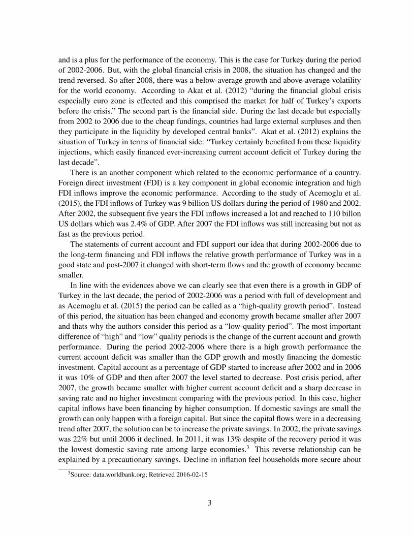
and is a plus for the performance of the economy. This is the case for Turkey during the periodof 2002-2006. But, with the global financial crisis in 2008, the situation has changed and thetrend reversed. So after 2008, there was a below-average growth and above-average volatilityfor the world economy. According to Akat et al. (2012) “during the financial global crisisespecially euro zone is effected and this comprised the market for half of Turkey’s exportsbefore the crisis.” The second part is the financial side. During the last decade but especiallyfrom 2002 to 2006 due to the cheap fundings, countries had large external surpluses and thenthey participate in the liquidity by developed central banks”. Akat et al. (2012) explains thesituation of Turkey in terms of financial side: “Turkey certainly benefited from these liquidityinjections, which easily financed ever-increasing current account deficit of Turkey during thelast decade”.

There is an another component which related to the economic performance of a country.Foreign direct investment (FDI) is a key component in global economic integration and highFDI inflows improve the economic performance. According to the study of Acemoglu et al.(2015), the FDI inflows of Turkey was 9 billion US dollars during the period of 1980 and 2002.After 2002, the subsequent five years the FDI inflows increased a lot and reached to 110 billonUS dollars which was 2.4% of GDP. After 2007 the FDI inflows was still increasing but not asfast as the previous period.

The statements of current account and FDI support our idea that during 2002-2006 due tothe long-term financing and FDI inflows the relative growth performance of Turkey was in agood state and post-2007 it changed with short-term flows and the growth of economy becamesmaller.

In line with the evidences above we can clearly see that even there is a growth in GDP ofTurkey in the last decade, the period of 2002-2006 was a period with full of development andas Acemoglu et al. (2015) the period can be called as a “high-quality growth period”. Insteadof this period, the situation has been changed and economy growth became smaller after 2007and thats why the authors consider this period as a “low-quality period”. The most importantdifference of “high” and “low” quality periods is the change of the current account and growthperformance. During the period 2002-2006 where there is a high growth performance thecurrent account deficit was smaller than the GDP growth and mostly financing the domesticinvestment. Capital account as a percentage of GDP started to increase after 2002 and in 2006it was 10% of GDP and then after 2007 the level started to decrease. Post crisis period, after2007, the growth became smaller with higher current account deficit and a sharp decrease insaving rate and no higher investment comparing with the previous period. In this case, highercapital inflows have been financing by higher consumption. If domestic savings are small thegrowth can only happen with a foreign capital. But since the capital flows were in a decreasingtrend after 2007, the solution can be to increase the private savings. In 2002, the private savingswas 22% but until 2006 it declined. In 2011, it was 13% despite of the recovery period it wasthe lowest domestic saving rate among large economies.3 This reverse relationship can beexplained by a precautionary savings. Decline in inflation feel households more secure about

3Source: data.worldbank.org; Retrieved 2016-02-15

3

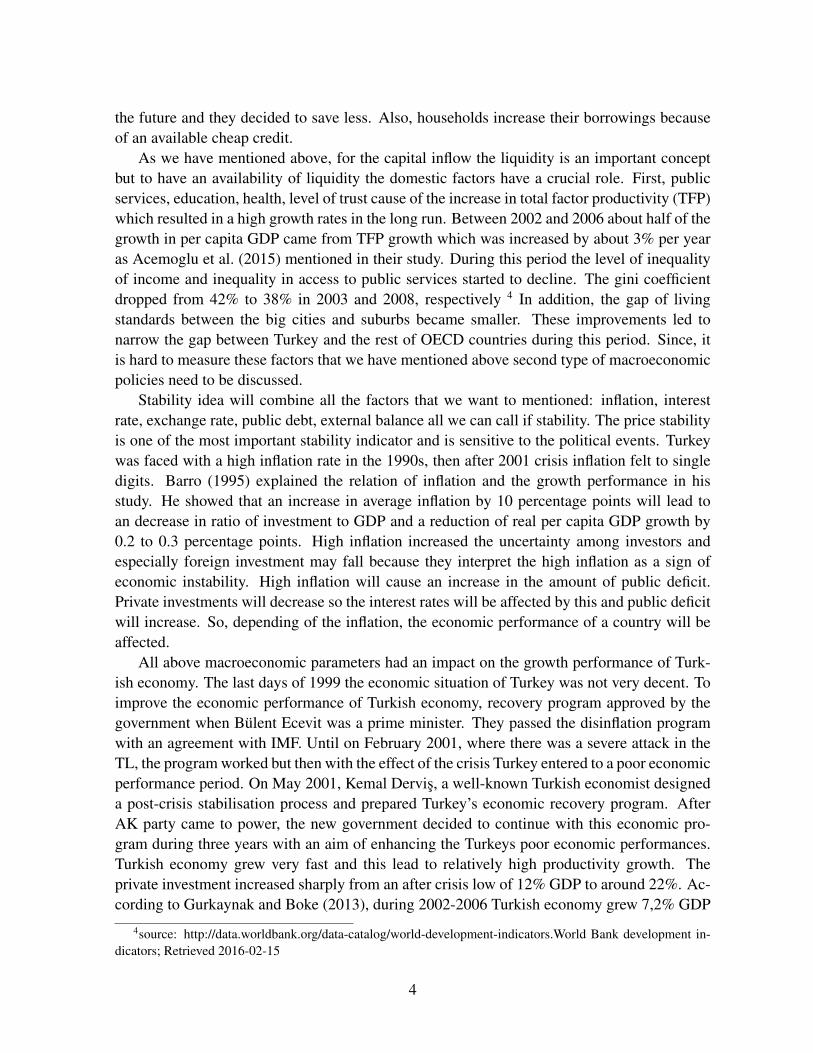
the future and they decided to save less. Also, households increase their borrowings becauseof an available cheap credit.

As we have mentioned above, for the capital inflow the liquidity is an important conceptbut to have an availability of liquidity the domestic factors have a crucial role. First, publicservices, education, health, level of trust cause of the increase in total factor productivity (TFP)which resulted in a high growth rates in the long run. Between 2002 and 2006 about half of thegrowth in per capita GDP came from TFP growth which was increased by about 3% per yearas Acemoglu et al. (2015) mentioned in their study. During this period the level of inequalityof income and inequality in access to public services started to decline. The gini coefficientdropped from 42% to 38% in 2003 and 2008, respectively 4 In addition, the gap of livingstandards between the big cities and suburbs became smaller. These improvements led tonarrow the gap between Turkey and the rest of OECD countries during this period. Since, itis hard to measure these factors that we have mentioned above second type of macroeconomicpolicies need to be discussed.

Stability idea will combine all the factors that we want to mentioned: inflation, interestrate, exchange rate, public debt, external balance all we can call if stability. The price stabilityis one of the most important stability indicator and is sensitive to the political events. Turkeywas faced with a high inflation rate in the 1990s, then after 2001 crisis inflation felt to singledigits. Barro (1995) explained the relation of inflation and the growth performance in hisstudy. He showed that an increase in average inflation by 10 percentage points will lead toan decrease in ratio of investment to GDP and a reduction of real per capita GDP growth by0.2 to 0.3 percentage points. High inflation increased the uncertainty among investors andespecially foreign investment may fall because they interpret the high inflation as a sign ofeconomic instability. High inflation will cause an increase in the amount of public deficit.Private investments will decrease so the interest rates will be affected by this and public deficitwill increase. So, depending of the inflation, the economic performance of a country will beaffected.

All above macroeconomic parameters had an impact on the growth performance of Turk-ish economy. The last days of 1999 the economic situation of Turkey was not very decent. Toimprove the economic performance of Turkish economy, recovery program approved by thegovernment when Bulent Ecevit was a prime minister. They passed the disinflation programwith an agreement with IMF. Until on February 2001, where there was a severe attack in theTL, the program worked but then with the effect of the crisis Turkey entered to a poor economicperformance period. On May 2001, Kemal Dervis, a well-known Turkish economist designeda post-crisis stabilisation process and prepared Turkey’s economic recovery program. AfterAK party came to power, the new government decided to continue with this economic pro-gram during three years with an aim of enhancing the Turkeys poor economic performances.Turkish economy grew very fast and this lead to relatively high productivity growth. Theprivate investment increased sharply from an after crisis low of 12% GDP to around 22%. Ac-cording to Gurkaynak and Boke (2013), during 2002-2006 Turkish economy grew 7,2% GDP

4source: http://data.worldbank.org/data-catalog/world-development-indicators.World Bank development in-dicators; Retrieved 2016-02-15

4

on average and this is the most important reason of the success of AK party in the electionsof 2007. (AK party won the elections with 40% majority.) Export oriented growth was alsoincreased.

According to the brief explanation about the Turkish economy above, we will focus on thelast 15 years of Turkish economy by separating the whole period into five sub-periods. To seethe before 2000 and to be able to compare the series we started from the second half of the1998 but the real analysis will start from the beginning of 2000. Starting from the beginning of2000, the first period will be until the 2001 crisis. Then, 2002-2006 period will be the secondsub period which is the first four years of AKP in power. As we have mentioned above, theTurkish economy started to change in 2007, so we will focus on 2007-2009 period, until theend of global crisis. Then, we call the 2010-2011 period as a recovery period. And, finally thelast three years, from 2012 to 2015.

We have examined the parameters that have an effect on growth and we commented on therecent Turkish economy using these parameters. Along with the macroeconomic perspectiveof Turkish economy there are many events which affects the performance of Turkish economyand the growth performance. We will not focus on all important events but some of them areremarkable for the sake of our study.

1.2 EventsTo understand the impact of an event on other economic entities of a country event studymethodology is used and it has many application areas to analyse the impact of the economicand political events. There are many event studies of Turkey to understand the effect of particu-lar events on the Turkish economy but up to our knowledge event studies generally choose onemarket index in isolation and doesn’t assume a network perspective which is lesser relevancefor our study.

An example of event study on Turkey, Mandaci (2003) analyzes the impact of generalelections on Turkish stock market between 1991 to 2002. They are based on the studies whichindicate that Istanbul stock exchange is not an efficient market and it is effected by the politicaland economic events. Their starting point is, under inefficient market conditions investorscould receive abnormal returns in this market and the abnormal returns are analyzed beforeand after the dates of general elections of Turkey. But they found that only in some electionsinvestors have been received abnormal returns in the market.

In another study Mutan et al. (2009) evaluate the impact of various 10 events from 1990to 2008 including economic, political events, terrorism and natural disaster, such as, economicpreventions in 1994, earthquake in 1999, economic crisis in 2001, terrorist attack to Britishconsulate in 2003. For all events, they interpreted the abnormal returns (AR) and the persis-tence of the change on the index. At the end they rank the events of AR and stated that onlysome events of AR have a significant meaning.

Unlike the studies above, the Chesney et al. (2010) emphasized the impact of 77 terroristattacks on stock, bond and commodity markets. They investigate the effect of terrorist attackson different areas, such as on global financial markets, travel industry, oil and gas industry, on

5

gold markets and bond markets. In addition, they analyzed if the effect of terrorist attacks onfinancial markets are similar with on natural disasters and financial crashes. They did not useonly event study methodology, also adopted non parametric tests and GARCH approaches tocompare the differences of results in various markets and they stated that the non-parametricapproach is the most appropriate one for their study. At the end, they found that approximatelytwo-thirds of terrorist attacks lead to significant negative impact on at least one stock market.Even they investigate the impact of events on several financial markets, their approach is em-phasising every market separately and evaluate the impact of events on every market. Theydid not focus on the interaction among financial markets which we are doing with networkperspective.

From 2000 to 2015 there are many important events that have an impact on Turkish econ-omy. For the last three years we will focus on the impact of these events using our method-ologies explained in Section 3 and the application of the methodologies in Section 4, 5 and6.

We will specify the most important events that have happened in Turkey in recent years.The most important events in the year 2013 was the Gezi Park protests and Corruption Scandal:

• Gezi Park Protests (2013-05-31): First wave of demonstrations have started as com-plaints against the planned construction of a shopping mall and a Taksim military bar-racks in the area of Gezi Park. Following days, the protests became wider and turnedto an antigovernment demonstrations. The increased tension of the police and protestersled to the protests quickly spreading all over Turkey, and turning into a protests to thecountry’s leaders from just an environmental movement. ”This was not an issue oftrees any more” and during the demonstrations 44 people had been injured.5. After onemonth, on July 2nd, a Turkish court has canceled the reconstruction of Gezi Parki andthe project.6

• 17/25 December, 2013, Corruption Scandal: Series of corruption investigations madepublic on Dec. 17 and 25, 2013, where several key people from Turkish government,including the son of the Prime Minister Recep Tayyip Erdogan, and many businessmanhave arrested. The investigations counted as the ”biggest corruption and bribery scandalin the history of the republic.”7

The noticeable events in 2014 are as follows:

• Repo rate increase: On January 28, the one-week repo rate was increased from 4.5% to10%, the overnight borrowing rate from 3.5% to 8% and the marginal funding rate from

5“Police Storm Park in Istanbul, Setting Off a Night of Chaos”, released 2016-01-22; available online athttp://www.nytimes.com/2013/06/16/world/europe/protesters-in-turkey.html

6“Turkish court blocks disputed park project”, released 2016-01-22; available online athttp://www.reuters.com/article/us-turkey-court-taksim-idUSBRE9620T220130703

7“Highlights of major corruption, bribery operations of Dec. 17, 25”, released 2016-01-23; availableonline at http://www.todayszaman.com/anasayfa highlights-of-major-corruption-bribery-operations-of-dec-17-25 357703.html

6

7.75% to 12%.8

• Local Elections: On 30 March 2014, the nationwide local elections were held in Turkey.Prime Minister’s party, Justice and Development Party (AKP) performed strongly in theelections and had over 45% of the vote.9 The local elections were an important testfor the AKP after the December 2013 corruption scandal. “One of the most interestingoutcomes of the elections, is that despite the recent corruption allegations, leaks andincreasing authoritarianism of the prime minister, AKP’s voters did not penalise theparty..”10

• First direct presidential election in Turkey: On 10 August 2014, first direct presiden-tial election was held to choose 12th president of Turkey. Recep Tayyip Erdogan wasselected the new president of Turkey with 51.95%.11

The important events happened in 2015:

• Turkish General Election: On 7 June 2015 Turkish general election took place to choose550 members to the Grand National Assembly. Since 2002, this was the first time thatJustice and Development party lost its parliamentary majority with a 40.9% of the vote.

• First operation to arrest the journalist from Gulen movement: On 14 December 2014Turkish police arrested more than 24 senior journalists and media executives connectedwith the Gulen movement. operation started with Zaman newspaper. Police was raidedthe Zaman newspaper and arrested the paper’s editor-in-chief Ekrem Dumanli.12

• Turkish General Elections: On 1 Nov 2015, the snap election was held to elect the newparliament of the country. After the election June 2015, the hung parliament’s coalitionnegotiations didn’t come to a conclusion and the President decided a snap election. TheJustice and Development Party regain the Parliamentary majority with 49.5% of the vote.

1.3 The present studyThe goal of this study is to assess the shock spillover characteristics of the Turkish stock marketsince 2000, with a view towards large-scale political and economic events within a network ofsix stock markets, each represented by a stock index, namely dji (USA), ftse (UK), sx5e (euro

8Official website of Turkish Central Bank, released 2016-01-23; http://www3.tcmb.gov.tr/yillikrapor/2014/en/m-0-2.php#1

9“A referendum on Erdogan’s rule”, released 2016-01-24; http://www.economist.com/blogs/charlemagne/2014/03/turkeys-local-elections

10“Turkish local elections: One victor, many losers”, released 2016-01-24;http://www.aljazeera.com/indepth/opinion/2014/04/turkish-local-elections-one-vict-20144211532875833.html

11“Erdogan emerges victorious in Turkish presidential elections a mid low turnout”, released 2016-01-25;http://www.theguardian.com/world/2014/aug/10/turkey-presidential-election-ergodan

12Turkey arrests: Raids target Gulen-linked critics of Erdogan, released 2016-01-25;http://www.bbc.com/news/world-europe-30468199

7

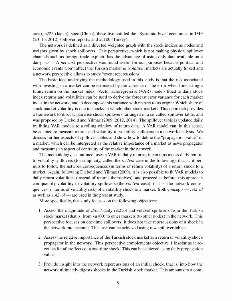
area), n225 (Japan), spec (China), these five entitled the “Systemic Five” economies in IMF(2011b, 2012) spillover reports, and xu100 (Turkey).

The network is defined as a directed weighted graph with the stock indices as nodes andweights given by shock spillovers. This perspective, which is not making physical spilloverchannels such as foreign trade explicit, has the advantage of using only data available on adaily basis. A network perspective was found useful for our purposes because political andeconomic events won’t affect the Turkish market in isolation; markets are actually linked anda network perspective allows to study “event repercussions”.

The basic idea underlying the methodology used in this study is that the risk associatedwith investing in a market can be estimated by the variance of the error when forecasting afuture return on the market index. Vector autoregressive (VAR) models fitted to daily stockindex returns and volatilities can be used to derive the forecast error variance for each marketindex in the network, and to decompose this variance with respect to its origin: Which share ofstock market volatility is due to shocks in which other stock market? This approach providesa framework to discuss pairwise shock spillovers, arranged in a so-called spillover table, andwas proposed by Diebold and Yilmaz (2009, 2012, 2014). The spillover table is updated dailyby fitting VAR models to a rolling window of return data. A VAR model can, in this sense,be adapted to measure return- and volatility-to-volatility spillovers in a network analysis. Wediscuss further aspects of spillover tables and show how to define the “propagation value” ofa market, which can be interpreted as the relative importance of a market as news propagatorand measures an aspect of centrality of the market in the network.

The methodology, as outlined, uses a VAR in daily returns; it can thus assess daily return-to-volatility spillovers (for simplicity, called the ret2vol case in the following), that is, it per-mits to follow the network consequences (in terms of return volatility) of a return shock to amarket. Again, following Diebold and Yilmaz (2009), it is also possible to fit VAR models todaily return volatilities (instead of returns themselves), and proceed as before; this approachcan quantify volatility-to-volatility spillovers (the vol2vol case), that is, the network conse-quences (in terms of volatility risk) of a volatility shock to a market. Both concepts — ret2volas well as vol2vol — are used in the present study.

More specifically, this study focuses on the following objectives:

1. Assess the magnitude of direct daily ret2vol and vol2vol spillovers from the Turkishstock market (that is, from xu100) to other markets (to other nodes) in the network. Thisperspective focuses on one-time spillovers; it does not take repercussions of a shock inthe network into account. This task can be achieved using raw spillover tables.

2. Assess the relative importance of the Turkish stock market as a return or volatility shockpropagator in the network. This perspective complements objective 1 insofar as it ac-counts for aftereffects of a one-time shock. This can be achieved using daily propagationvalues.

3. Provide insight into the network repercussions of an initial shock, that is, into how thenetwork ultimately digests shocks in the Turkish stock market. This amounts to a com-

8

parison of network importance (objective 2) and direct spillovers (objective 1). This canbe achieved by regressing propagation values on direct spillovers.

Consequently, this paper continues with the empirical data (essentially, daily stock indexquotations from six markets) used in the present study in Section 2. In Section 3, we firstreview the theory underlying the spillover perspective (objective 1 above) and then introducefurther methodology to discuss objectives 2 and 3. The subsequent sections report and discussempirical results concerning objective 1 (Section 4), objective 2 (Section 5), and objective 3(Section 6). Section 7 summarizes and concludes the paper. — All computations were carriedout with scripts written in R (2015).

2 DataThe empirical starting point of the present study consists of daily closing quotations of theTurkish stock index (xu100) and the five stock indices representing stock markets in the “Sys-temic Five” countries: Dow Jones Industrial Average (USA; dji), FTSE (UK; ftse), EuroStoxx 50 (euro area; sx5e), Nikkei 225 (Japan; n225), and SSE Composite (China; ssec).The series begin with 1998-03-03 (the first day for which all six series were available) and endwith 2016-03-18 (4696 observations). The series of daily simple returns in percent are plottedin Figure 1.

Obtaining daily volatilities is a prerequisite for investigating vol2vol spillovers. This re-quires further daily data, namely opening, high, and low, in addition to daily closing quota-tions. The corresponding series are not plotted here.

−20

020

dji

−20

020

ftse

−20

020

sx5e

−20

020

n225

−20

020

ssec

−20

020

xu10

0

1998 2000 2002 2004 2006 2008 2010 2012 2014 2016

Figure 1: The series of daily returns

9

3 Measuring spillovers and shock repercussions

3.1 Return-to-volatility spillovers (“ret2vol”)Direct spilloversLet (xkt)t=1,...,T , where k = 1, . . . , N , designate N series of daily price changes (simple re-turns in percent); N is the number of stock markets in the network. The methodology usedin the present paper builds on the spillover matrix by Diebold and Yilmaz (2009, 2014) andextensions developed in Schmidbauer et al. (2013b). For a given day t, the spillover matrixis a matrix M = (mik)i,k=1,...,N (we drop the index t, for ease of exposition) with row sumsequal to one, that is,

∑Nk=1mik = 1, where each row (mi1, . . . ,miN) provides a breakdown of

the forecast error variance of xi into shares with respect to its origin. In this sense, mik is theshare of variability in xi due to shocks in xk. For example, in the case of N = 3 markets, aspillover matrix

M =

0.6 0.2 0.2

0.1 0.6 0.3

0.1 0.3 0.6

, (1)

means that 60% (20% each) of forecast error variance of x1 is due to shocks in x1 itself (shocksin x2 and x3, respectively). In other words: 40% of the volatility in market 1 is due to spilloversto market 1 from markets 2 and 3. Considering the first column of M, an “aggregate share”(column sums need not add up to 1) of 0.2 is spilled over from market 1 to markets 2 and 3,making market 1 a net receiver. Market 2 is a net giver.

Direct spillovers from market k (or to market i) are then given by the column (row, respec-tively) sums in M, excluding the market’s spillovers to itself:13

from market k to others:N∑

i=1,i 6=k

mik; to market i from others:N∑

k=1,k 6=i

mik (2)

In social network terminology, with M interpreted as adjacency matrix of a weighted directednetwork of nodes, these aggregates are the from-degree of node k (to-degree of node i, respec-tively); see Diebold and Yilmaz (2014).

For a given day t, the spillover matrix M is obtained as follows: Fit a standard VARmodel of order 1 to the N return series, using data from a window of size 100 (that is, dayst − 99, . . . , t). We follow Diebold and Yilmaz (2014) and use an approach suggested by ?,namely: to identify the impulse response function of a component (here, xk), give highestpriority to that component; this removes the dependence on an imposed hierarchy of markets.Forecasting n steps ahead (we use n = 5), forecast error variance decomposition (fevd) yieldsforecast error variance shares (mi1, . . . ,miN). This procedure is then applied for every t,resulting in a sequence of spillover matrices.

Relative importance of a market: propagation values13Spillovers from market k to others, plus spillovers to itself, need not sum up to 1.

10

The network structure of the spillover matrix with respect to the propagation of shocks lendsitself to a broader perspective, elaborated in Schmidbauer et al. (2013b). Let M again denotethe spillover matrix for day t. We assume that M contains all relevant, and the most recentavailable, information about the network. A hypothetical shock (“news”, “information”) ofunit size in market k on day t can be denoted as n0 = (0, . . . , 0, 1, 0, . . . , 0)′, where 1 is in thek-th component of n0. We assume that the propagation of this shock across the markets withinday t will take place in short time intervals of unspecified length according to

ns+1 = M · ns, s = 0, 1, 2, . . . (3)

(where step s = 0 initializes the recursion). The index s in Equation (3) therefore denotesa step in information flow. Moreover, assuming that information flow across markets canproceed instantly on day t, with spillover conditions (given by M) persisting throughout day t,it makes sense to investigate steady-state properties (as s → ∞) of the model defined byEquation (3). This leads to

v′ = v′ ·M. (4)

When the left eigenvector v = (v1, . . . , vN)′ is normed such that

∑Nk=1 vk = 1, we call vk the

propagation value of market k. It renders the value of a return shock in market k as seed forfuture uncertainty in returns across the network of markets:

vk =N∑i=1

mik · vi (5)

For M as in Equation (1), v′ = (0.2, 0.4, 0.4), which means that a shock in market 2 is twiceas powerful (0.4/0.2 = 2) as a shock in market 1 in terms of creating network volatility. —A similar concept, eigenvector centrality, is also used in social network analysis; see, forexample,Bonacich (1987).

Network repercussions of a shockDirect spillovers from market k to others measure the direct impact of a shock in xk on day t,without consideration of immediate (that is, also happening on day t) network repercussionsof the shock. The propagation value of market k, in contrast, emphasizes the importance ofshocks in xk within the network, including repercussions throughout the network. Owingto different magnitudes, direct spillovers from market k and propagation values of market kcannot be directly compared. However, they can be related to each other via a regression

propagation value t = α + β · spillover t + εt, (6)

where propagation value t (spillover t) denote the propagation value of market k (direct spilloversfrom market k, respectively) on day t. The residuals εt can be interpreted as propagation values(or relative network importance) of market k, from which direct spillovers have been compu-tationally removed. What remains is a measure of network repercussions of a direct spillover,that is: the repercussions of a one-time shock in market k throughout the network, once again

11

assuming that the spillover matrix is the only relevant information structure for a given day.Therefore, εt indicates which effect is prevailing:

εt

{> 0 : network repercussions are more important than direct spillovers on day t,< 0 : direct spillovers have little repercussions in the network on day t.

(7)

This methodology will be applied in Section 6, where market k designates the Turkish stockmarket.

3.2 Volatility-to-volatility spillovers (“vol2vol”)The methodology outlined in Section 3.1 can also be applied to a set of series (xkt)t=1,...,T ofdaily volatilities, instead of returns (Diebold and Yilmaz, 2009). One difficulty to overcomeis that daily volatilities cannot be directly observed and need to be reconstructed. Follow-ing Diebold and Yilmaz (2009), we use a method proposed by Garman and Klass (1980),based on the hypothesis that the stock price process is a geometric Brownian motion, to obtaindaily variances. Their method results in the following formula:

σ2t = 0.511(Ht − Lt)

2

−0.019[(Ct −Ot)(Ht + Lt − 2Ot)− 2(Ht −Ot)(Lt −Ot)]

−0.383(Ct −Ot)2,

(8)

where Ot (Ht, Lt, Ct) designate the natural logarithm of the daily opening price (daily high,daily low, daily closing, respectively) on day t. After obtaining a daily variance series for eachmarket considered, a sequence of spillover matrices — updated daily — can be computed,leading to daily direct spillovers as well as to daily propagation values. In this case, directspillovers characterize volatility-to-volatility spillovers, while the propagation values quantifythe importance of a market with respect to the propagation of a volatility shock across mar-kets, that is, the value of a volatility shock from that market as seed for future uncertainty involatility across the network of markets.

The methodology outlined in this section will now be applied to the data described inSection 2. In view of our focus on the Turkish economic history, results will be reported anddiscussed in the following three sections.

12

4 Direct spillovers from and to xu100This section reports the first part of spillover characteristics of the Turkish stock market,namely direct return and volatility spillovers, without considering potential aftereffects of ashock. The subsequent Section 5 and 6 will give more detailed interpretations, using themethodological innovations (propagation values and network repercussions) introduced inSection 3.1 and 3.2. Attention will be given to the following periods and events which haveexplained above in detail. Same periods also will be examined in Section 5 and 6.

• Period 1 (roughly, July 1998 - end of 2002): Period covers the pre and post periods ofcrisis in 2001, which started in the first half of 2001. On February 2001 the financialcrisis started and on May 2001 a new economic program established to stabilise the postcrisis period. In addition, on August 1999, a severe earthquake took place in Turkeywith an extensive damage and killing around 17.000 people in terms of reports. Periodends at the beginning of 2002 where the new program endorsed by IMF and World Bankstarted to take an effect and some structural changes started.

• Period 2 (roughly, beginning of 2002 - end of 2006): The period was full of developmentand the growth performance of Turkish economy was very high during these 4 fouryears. On November 2002, general elections took place in Turkey and AKP was inpower in the first time.

• Period 3 (roughly, beginning of 2007 - end of 2009): The period started at the turnoverpoint of Turkish economy which was the beginning of 2007. Almost all economic indi-cators started to change and the successful days from 2002-2006 has remained behind.The period continued with the global financial crisis which lasted until the second halfof 2009.

• Period 4 (roughly, beginnning of 2010 - end of 2012): After the crisis the recovery periodhas started for the Turkish economy. Even if it was not as good as the 2002-2006 period,the economy started to grow again.

• Period 5 (roughly, beginning of 2013 - beginning of 2016): The growth performanceof Turkish economy became smaller. Important events happened during this periodand especially Gezi park protests and 17/25 December corruption scandal had a severeimpact on Turkish economy.

4.1 The case return-to-volatility (ret2vol)The daily series of direct return spillovers from xu100 to others and from others to xu100are displayed in Figure 2. Return spillovers to xu100 have always been higher than returnspillovers from xu100 from the beginning to the end of 2006. So, the Turkish market has beena net receiver of return shocks before 2007. But after the third period the story has started tochange and from xu100 exceeded in some intervals. In period 5, where it started from 2012,

13

Turkish market again became a net receiver with a higher ‘to xu100’ direct spillovers. Inaddition, the character of the spillover index was changed after 2007. The whole period can bedivided into two sub periods: before and after 2007. Both spillovers were more volatile before2007 and the connectedness is low during this period. But, after 2007, the fluctuations becamesmaller and the connectedness increased. Further observations about the period specific directspillovers are as follows:

• Period 1: The first half of the 1999, both from and to spillovers increased and theymoved together. On August 1999, both spillovers went down sharply which coinsideswith the days of a severe earthquake in Turkey. Until the beginning of 2001 from and toreturn spillovers are in a similar pattern and both in a very low level. On February 2001,to xu100 received a significant boost, which is the first days of the financial crisis, whilespillovers from xu100 was not responded to this event immediately but both started toincrease after a couple of days.

• Period 2: The direct spillovers was still in a volatile period. There were no big spikesduring this period but from and to spillovers was in an increasing trend and continued torise until the end of the period. Since during the whole period to xu100 direct spilloverswere higher than from xu100 spillovers Turkey was a net receiver of return shocks whenthe Turkish economy was improving and the growth performance was very high.

• Period 3: In the whole period the spillovers were higher than other periods and at thebeginning of 2008 the direct return spillovers was in its peak value. This means thatTurkey was much more integrated in this period than before. Since the level was verylow before, Turkey started to grown up with the beginning of the third period, on 2007.On mid-2008, there was a sharp decrease on both return spillovers, but especially fromxu100 was responded more to the shocks. It decreased from 50 to 15 level on mid-2008where the global financial crisis has started.

• Period 4: The gap between from and to return spillovers was very narrow in period4. During the recovery period, the spillovers was lower than period 3 but still with aremarkably high level. Both spillovers decreased on 2011 for a short period of time butat the second half of 2011 it reached again to high levels.

• Period 5: Starting from 2012 the spillovers were in a decreasing trend and the overallperiod the spillover level was lower than in period 3 and 4. There were two spikes duringthe whole period where the first one coincides with the Gezi park protests on May 2013and the second one with the corruption scandal on December 2014 but the responses tothis events was not very high for the return spillovers cases.

4.2 The case volatility-to-volatility (vol2vol)The daily series of direct volatility spillovers from xu100 to others and from others to xu100are displayed in Figure 3. Volatility spillover patterns are more distinct than those of return

14

spillovers, and they are different. Like in the return case, on general the Turkish market canbe counted as a net receiver of volatility spillover. The pattern of volatility spillovers was verydifferent than the return and some fluctuations can be related with certain events which can notbe distinguished in the return spillover case.

• Period 1: As we have mentioned in the return spillovers, in mid-1999 there were a sharpdecrease in return spillovers which coincides with the earthquake disaster in Turkey. Thesharp decrease was observable in from xu100 volatility spillovers unlike the return. Atthe beginning of 2000, both volatility spillovers started to increase.

• Period 2: The whole period was with a lot of fluctuations and the direct spillovers waslower comparing with the other periods. From and to direct spillovers were differentand they were not move together, so we cannot distinguish if the Turkish market is netreceiver or net sender for this period unlike the return case. Starting from 2004 bothspillovers started to increase where the growth of the Turkish economy began faster.

• Period 3: With the third period the story has changed and the volatility spillovers hadless fluctuations and the level increased. Unlike in the return spillovers, the volatilityones are still distinct and from xu100 spillovers did their peak value in the beginning of2008. After a sharp increase, both spillovers drop to their average value of this periodand this drop coincides with the days of global financial crisis.

• Period 4: The gap between from and to spillovers was still large and from xu100spillovers have much more fluctuations than the returns. As we have mentioned in theintroduction part we can call the period as a recovery period for Turkish economy. Thespillovers was not very high but starting from 2011 they were in an increasing trend.

• Period 5: The from and to spillovers still had fluctuations especially from xu100 spillovershad many. The biggest spike was at the end of May 2013, from xu100 received a sig-nificant boost at this date, which is the first weekday after the Gezi park protests. Thefrom and to return spillovers was less responded to this event unlike the from volatilityspillover. Later 2014, a huge drop happened in both volatility spillovers and it stayedalmost the same level for a couple of days and then gradually increased. The drop ofspillovers coincide with the date of corruption scandal on December 2014 while theeffect was not distinguishable for the return spillovers.

4.3 DiscussionDuring the whole period, although the return and volatility spillovers had different characters,both has responsed to the political and economic events. We can clearly deduce that even returnand volatility spillovers had different amount of responses to the different events the spilloversare period specific and the political events impact the stock market network characteristics.The pattern of return spillovers for from and to xu100 was very similar and they were generallymoved in a same direction during the whole period. The ret2vol spillovers indicate that Turkey

15

is much more integrated to the network after 2007, where the level of spillovers increased andthere were less fluctuations in direct spillovers. Unlike the return, it is harder to analysis theprocess of volatility spillovers, from and to xu100 patterns are distinct and they were not movetogether. But, unlike the return spillovers the responses to a political or economic event ismuch more clear in the volatility spillover case.

16

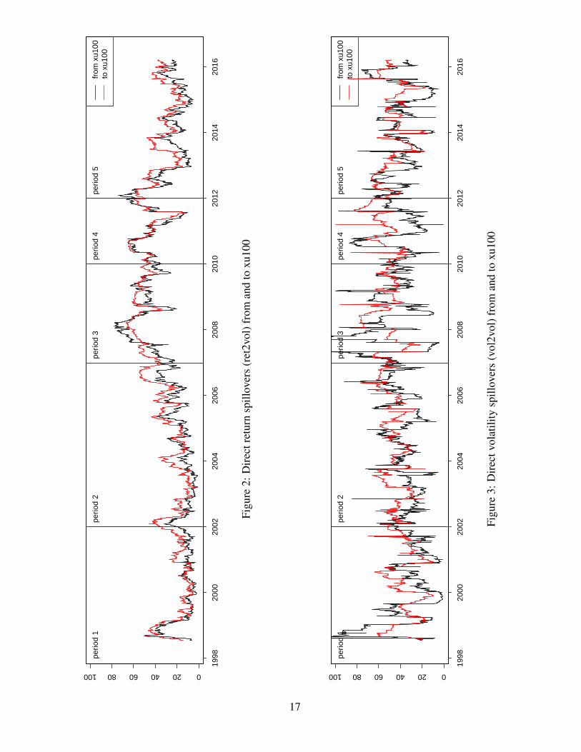
020406080100

1998

2000

2002

2004

2006

2008

2010

2012

2014

2016

perio

d 1

perio

d 2

perio

d 3

perio

d 4

perio

d 5

from

xu1

00to

xu1

00

Figu

re2:

Dir

ectr

etur

nsp

illov

ers

(ret

2vol

)fro

man

dto

xu10

0

020406080100

1998

2000

2002

2004

2006

2008

2010

2012

2014

2016

perio

d 1

perio

d 2

perio

d 3

perio

d 4

perio

d 5

from

xu1

00to

xu1

00

Figu

re3:

Dir

ectv

olat

ility

spill

over

s(v

ol2v

ol)f

rom

and

toxu

100

17

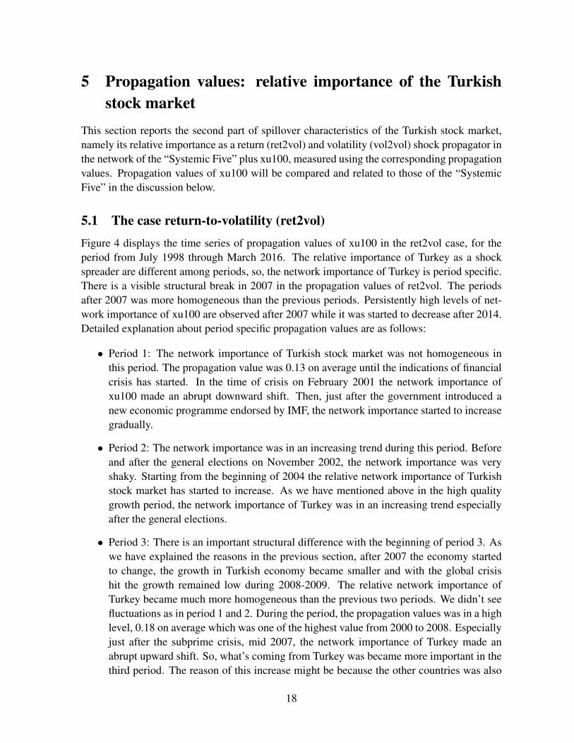
5 Propagation values: relative importance of the Turkishstock market

This section reports the second part of spillover characteristics of the Turkish stock market,namely its relative importance as a return (ret2vol) and volatility (vol2vol) shock propagator inthe network of the “Systemic Five” plus xu100, measured using the corresponding propagationvalues. Propagation values of xu100 will be compared and related to those of the “SystemicFive” in the discussion below.

5.1 The case return-to-volatility (ret2vol)Figure 4 displays the time series of propagation values of xu100 in the ret2vol case, for theperiod from July 1998 through March 2016. The relative importance of Turkey as a shockspreader are different among periods, so, the network importance of Turkey is period specific.There is a visible structural break in 2007 in the propagation values of ret2vol. The periodsafter 2007 was more homogeneous than the previous periods. Persistently high levels of net-work importance of xu100 are observed after 2007 while it was started to decrease after 2014.Detailed explanation about period specific propagation values are as follows:

• Period 1: The network importance of Turkish stock market was not homogeneous inthis period. The propagation value was 0.13 on average until the indications of financialcrisis has started. In the time of crisis on February 2001 the network importance ofxu100 made an abrupt downward shift. Then, just after the government introduced anew economic programme endorsed by IMF, the network importance started to increasegradually.

• Period 2: The network importance was in an increasing trend during this period. Beforeand after the general elections on November 2002, the network importance was veryshaky. Starting from the beginning of 2004 the relative network importance of Turkishstock market has started to increase. As we have mentioned above in the high qualitygrowth period, the network importance of Turkey was in an increasing trend especiallyafter the general elections.

• Period 3: There is an important structural difference with the beginning of period 3. Aswe have explained the reasons in the previous section, after 2007 the economy startedto change, the growth in Turkish economy became smaller and with the global crisishit the growth remained low during 2008-2009. The relative network importance ofTurkey became much more homogeneous than the previous two periods. We didn’t seefluctuations as in period 1 and 2. During the period, the propagation values was in a highlevel, 0.18 on average which was one of the highest value from 2000 to 2008. Especiallyjust after the subprime crisis, mid 2007, the network importance of Turkey made anabrupt upward shift. So, what’s coming from Turkey was became more important in thethird period. The reason of this increase might be because the other countries was also

18

struggling with the global financial crisis, and because the others was more shaky, theimportance of Turkish stock market was increased.

• Period 4: Starting with the 2010 the recovery days for Turkish economy was started.The propagation value was still homogeneous like the previous period and it remainedpretty much constant during the whole period.

• Period 5: At the beginning of the period the network importance of Turkish stock marketwas in a despising trend, as we know from the economic history that explained in theprevious sections the growth performance of Turkish economy is smaller during thebeginning of the period. Persistently high levels of network importance of xu100 areobserved in the first half of 2014. The maximum network importance for this periodwas in the beginning of June 2013 which coincides with the Gezi Park protests. Justafter the Gezi park protests the network importance of xu100 rose sharply and duringthe protests week it stays in a very high level than before. Then mid-june the networkimportance of Turkey fall their beginning of May 2013 level with a little upward shift.On the December 16, the structure of the propagation value has changed and becamevolatile which coincides with the beginning of the corruption scandal, on December 17.So, for 2013 we can say that in two cases the propagation value has an important changein its structure. From mid 2013 the network importance was started to increase evenit was more volatile during the corruption scandal, it was in an increasing trend. AfterDecember 2014 the propagation value became stable until the beginning of June whichcoincides with the date of general elections on Turkey. On 2015, the propagation valuewas in an increasing trend and more volatile. The sharp decline on 2015 coincides thedate of general elections on June 2015.

5.2 The case volatility-to-volatility (vol2vol)The character of the propagation values of xu100 in the vol2vol case was different than theret2vol. In volatility case the network importance of Turkey has much more fluctuations thanthe return case. In the first two periods the relative market importance of Turkey has manyspikes and it was not homogeneous. After 2007, even the structural break is not clear as in thereturn case, starting with period 3 the network importance is less heterogeneous.

• Period 1: The network importance of Turkish stock market had many fluctuations inthis period. The relative network importance was very little at the beginning of 2000but it started to increase gradually until the beginning of 2001 where the financial crisisstarted. The network importance of Turkey was relatively high before the crisis but im-mediately after the crisis the importance disappeared. Until the beginning of 2002 wherethe Turkish economy started to improve, the relative network importance of Turkey wasnot high but after 2002 it entered into an increasing trend.

• Period 2: The network importance was in an increasing trend for the whole period. Asin the return case, the relative network importance of Turkey was very shaky, before and

19

after the general elections. Especially after the general elections in 2002 the relativenetwork importance was its highest value from the beginning. Starting from the begin-ning of 2005 the propagation value was started to rise and became more homogeneous.As we mentioned in the introduction part the economy was in a good situation and thegrowth rate of Turkey was high during the period of 2002-2006, the network importanceof Turkey was increasing in this period. So, among all the countries the importance ofTurkish market in the network is more important then in the previous periods.

• Period 3: As we have mentioned above the 2007 was an important year in the Turkisheconomic history. The successful periods started to became an end with a forthcomingcrisis. As in the return case there is a structural change in the network importance ofTurkey. The propagation value of Turkey in the volatility case was not calmer as inthe return, there were still big spikes but it was more homogeneous. Starting from themid 2007, the relative importance of Turkey was decreasing which coincides with thesubprime crisis. But after 2008, where the global financial crisis has started, althoughTurkey was also affected from the crisis, the propagation values was increasing. Whatwas coming from Turkey was became more important after the global financial crisis.Since, the other network member was also affected from the financial crisis it worthlook at the general relative network importance of all markets and examine the reasonof the behaviour of the propagation value in this period. The analysis will be done in thediscussion part of this section.

• Period 4: During the recovery days of the Turkey the propagation values was not veryhigh. Staring from mid-2011 it started to increase.

• Period 5: During 2012 the propagation value did not changed. Since the beginning ofthe period the growth performance of Turkish economy became smaller, there were nosuch big changes in terms of the relative importance. At the first days of June 2013,the relative market importance did a huge jump and the network importance was in itsmaximum value which is the date of the first weekday after the Gezi park protests. Justafter the Gezi park protests the network importance of xu100 rose sharply and duringthe next two week it stayed in a high level. Until the end of 2013 the relative networkimportance was in a shaky level. During the second half of 2013, the network importanceif Turkey was very volatile which period includes the corruption scandal on December17. Starting from mid 2015 the network importance was in an increasing trend until thebeginning of 2016.

5.3 DiscussionWe find evidence from the ret2vol and vol2vol propagation values that we can define sub-periods where the relative importance of Turkey as a new spreader are distinct. Turkey as ashock spreader changed during the periods. Even the ret2vol and vol2vol propagation valueshad different pattern in the whole interval they have similarities in terms of breakpoints and

20

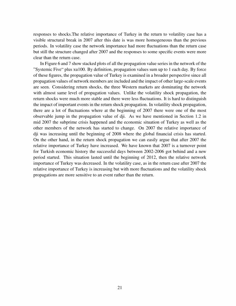
responses to shocks.The relative importance of Turkey in the return to volatility case has avisible structural break in 2007 after this date is was more homogeneous than the previousperiods. In volatility case the network importance had more fluctuations than the return casebut still the structure changed after 2007 and the responses to some specific events were moreclear than the return case.

In Figure 6 and 7 show stacked plots of all the propagation value series in the network of the”Systemic Five“ plus xu100. By definition, propagation values sum up to 1 each day. By forceof these figures, the propagation value of Turkey is examined in a broader perspective since allpropagation values of network members are included and the impact of other large-scale eventsare seen. Considering return shocks, the three Western markets are dominating the networkwith almost same level of propagation values. Unlike the volatility shock propagation, thereturn shocks were much more stable and there were less fluctuations. It is hard to distinguishthe impact of important events in the return shock propagation. In volatility shock propagation,there are a lot of fluctuations where at the beginning of 2007 there were one of the mostobservable jump in the propagation value of dji. As we have mentioned in Section 1.2 inmid 2007 the subprime crisis happened and the economic situation of Turkey as well as theother members of the network has started to change. On 2007 the relative importance ofdji was increasing until the beginning of 2008 where the global financial crisis has started.On the other hand, in the return shock propagation we can easily argue that after 2007 therelative importance of Turkey have increased. We have known that 2007 is a turnover pointfor Turkish economic history the successful days between 2002-2006 got behind and a newperiod started. This situation lasted until the beginning of 2012, then the relative networkimportance of Turkey was decreased. In the volatility case, as in the return case after 2007 therelative importance of Turkey is increasing but with more fluctuations and the volatility shockpropagations are more sensitive to an event rather than the return.

21

0.000.100.200.30

1998

2000

2002

2004

2006

2008

2010

2012

2014

2016

perio

d 1

perio

d 2

perio

d 3

perio

d 4

perio

d 5

Figu

re4:

Prop

agat

ion

valu

esof

xu10

0,re

t2vo

l

0.000.100.200.30

1998

2000

2002

2004

2006

2008

2010

2012

2014

2016

perio

d 1

perio

d 2

perio

d 3

perio

d 4

perio

d 5

Figu

re5:

Prop

agat

ion

valu

esof

rts,

vol2

vol

22

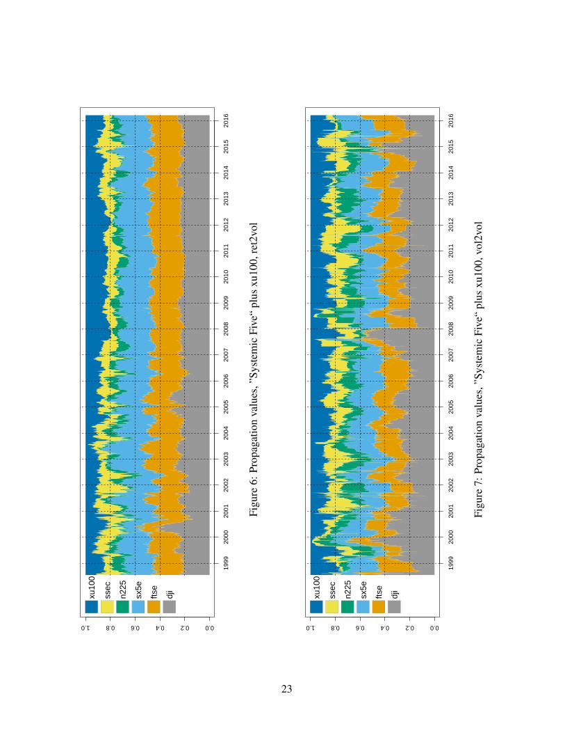
0.00.20.40.60.81.0

1999

2000

2001

2002

2003

2004

2005

2006

2007

2008

2009

2010

2011

2012

2013

2014

2015

2016

xu10

0

ssec

n225

sx5e

ftse

dji

Figu

re6:

Prop

agat

ion

valu

es,”

Syst

emic

Five

“pl

usxu

100,

ret2

vol

0.00.20.40.60.81.0

1999

2000

2001

2002

2003

2004

2005

2006

2007

2008

2009

2010

2011

2012

2013

2014

2015

2016

xu10

0

ssec

n225

sx5e

ftse

dji

Figu

re7:

Prop

agat

ion

valu

es,”

Syst

emic

Five

“pl

usxu

100,

vol2

vol

23

6 Network repercussions of shocks in the Turkish marketThe section reports the third part of spillover characteristics of the Turkish stock market,namely network repercussions of return and volatility shocks in the Turkish market. Directspillovers from the Turkish market as well as the market’s propagation values have a distinctperiod-specific behaviour. Even they have similar pattens at first sight, there are differencesbetween them. As was pointed out in Section 3, a direct comparison of both series is notmeaningful, while regression residuals are able to release whether direct spillovers or networkimportance surpass at a given time. A residual close to zero indicates that direct spilloversand network importance are equal, while positive (negative) residuals indicate that networkimportance (direct spillovers) outweighs directs spillovers (network importance, respectively).The two residual series (εt), one for each spillover perspective, are plotted in Figures 8 and 9from 1998 to 2016. The standardised series will be analysed in the following.

6.1 The case return-to-volatility (ret2vol)In Figure 8 the network repercussions of return shocks is shown. As in the propagation valuesand spillover index, we can distinguish two different behaviour in the network repercussion atfirst sight: before and after 2007. Even if the most visible structural change was before andafter 2007, every period has its own character which is explained as follows:

• Period 1: The first period is very shaky in terms of network repercussions and generallyit is above the zero level. During the first period, the network repercussions of Turkeyare generally more important than spillovers from Turkey to others. The beginning of theperiod the regression residuals was a level of zero but with an increasing trend. Startingfrom 2000, the network importance increasing so Turkish stock market started to leaveeffects on the network. Until the end of 2000, the network repercussion of Turkey wasalways above zero. At the beginning of October 2000, the repercussion of return shockjumped and reached in its maximum level in the whole period. Starting from 2001,which coincides with the beginning of financial crisis, the network repercussions lowerand even below zero, which means that direct spillovers from Turkey is dominated butnetwork ignores it.

• Period 2: The second period was similar to the first one in terms of fluctuations but thequantity is less than the first one. The repercussions of a return shock from Turkey is notstable during the period from 2002 to 2006. Like in the previous period there are jumpsand drops which coincides the shiny periods for the Turkish economy.

• Period 3,4 and 5: There is a huge difference in the network repercussions starting fromthe third period. The character of repercussions completely changed and it became muchmore stable than before. There were not big jumps and drops after 2007 and the levelis always around zero. So, after 2007, where we knows that the economy getting worsecomparing with the period 2002-2006, direct spillovers and network importance are ona par and neither of them were dominated.

24

6.2 The case volatility-to-volatility (vol2vol)The plot of network repercussions of volatility shocks is shown in Figure 9. Unlike the reper-cussions in return shocks, the series of regression residuals are close to zero, except a lot ofspikes during the period. Although there are more jumps in the volatility case, except thejumps, the residuals are almost always are on the level of zero. The repercussions in volatil-ity case are tend to have big spikes rather than drops. In addition, in the volatility case it isharder to distinguish a structural change among periods as it was in the return case. The periodspecific vol-to-vol repercussions and examination of booms for each period are as follows:

• Period 1: The whole period the vol-to-vol network repercussions are generally abovezero level which means that the network importance are more important than spilloversfrom Turkey. The biggest spike in this period was in November 22, 2000 with a value of9.4 and the second one in February 22, 2001 with a value of 4.9. So within the networkthe importance of Turkey is high especially for this two cases and the network cannotdigest this importance immediately. Network was not ready to face with the shock thatcame from Turkey. The spots with an important jump in network repercussions coincideswith the beginning of the financial crisis in Turkey. The second peak in February 22,2001 was the days of financial crisis where the Turkish economy affected seriously andit produces shocks within the network.

• Period 2: The character of the second period was similar to the previous one, the networkrepercussions the level is generally close to zero with some spikes during the period.There were two important spikes; the first one was on 2002-11-08 which is just afterthe general elections in Turkey. On 2002-11-03 was the day of general elections wherethe Justice and Development Party was in power in the first time. The second day wason 2003-10-07 which coincides with the day of permitting to send troops to Irak wasaccepted by the Turkish government.

• Period 3 and 4: The character of the network repercussions has changed although it wasnot as obvious as in the return case. The level was again around zero but unlike theprevious period the repercussions was less shaky and the number of jumps are less thanthe previous periods. The character was similar in period 3 and 4 and there were onlyone jump on 2007-04-30.

• Period 5: The character was not different than the previous two periods but it was moreshaky and with more jumps. The most important date of this period was on 2013-05-31which is the day of Gezi park protests an important day for Turkish history. The networkrepercussions was at its peak value on 2013-06-03, which is the first week day after theGezi protests. It was a big surprise for the network and network was not ready for sucha huge shock.

25

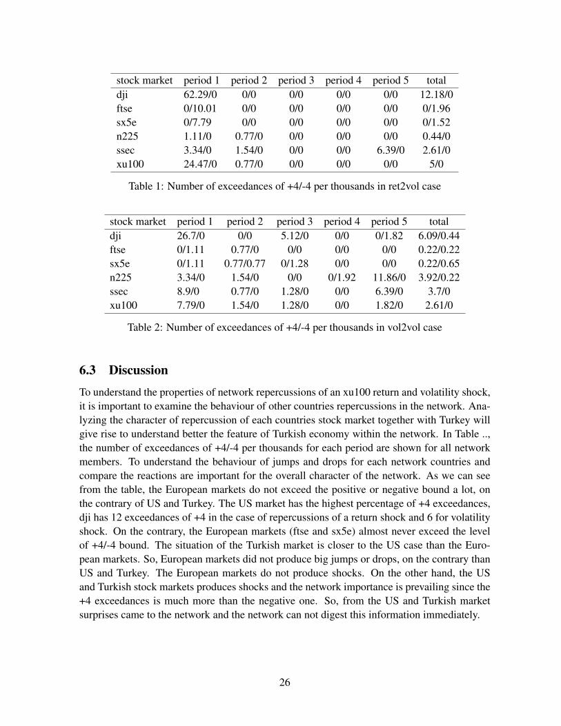
stock market period 1 period 2 period 3 period 4 period 5 totaldji 62.29/0 0/0 0/0 0/0 0/0 12.18/0ftse 0/10.01 0/0 0/0 0/0 0/0 0/1.96sx5e 0/7.79 0/0 0/0 0/0 0/0 0/1.52n225 1.11/0 0.77/0 0/0 0/0 0/0 0.44/0ssec 3.34/0 1.54/0 0/0 0/0 6.39/0 2.61/0xu100 24.47/0 0.77/0 0/0 0/0 0/0 5/0

Table 1: Number of exceedances of +4/-4 per thousands in ret2vol case

stock market period 1 period 2 period 3 period 4 period 5 totaldji 26.7/0 0/0 5.12/0 0/0 0/1.82 6.09/0.44ftse 0/1.11 0.77/0 0/0 0/0 0/0 0.22/0.22sx5e 0/1.11 0.77/0.77 0/1.28 0/0 0/0 0.22/0.65n225 3.34/0 1.54/0 0/0 0/1.92 11.86/0 3.92/0.22ssec 8.9/0 0.77/0 1.28/0 0/0 6.39/0 3.7/0xu100 7.79/0 1.54/0 1.28/0 0/0 1.82/0 2.61/0

Table 2: Number of exceedances of +4/-4 per thousands in vol2vol case

6.3 DiscussionTo understand the properties of network repercussions of an xu100 return and volatility shock,it is important to examine the behaviour of other countries repercussions in the network. Ana-lyzing the character of repercussion of each countries stock market together with Turkey willgive rise to understand better the feature of Turkish economy within the network. In Table ..,the number of exceedances of +4/-4 per thousands for each period are shown for all networkmembers. To understand the behaviour of jumps and drops for each network countries andcompare the reactions are important for the overall character of the network. As we can seefrom the table, the European markets do not exceed the positive or negative bound a lot, onthe contrary of US and Turkey. The US market has the highest percentage of +4 exceedances,dji has 12 exceedances of +4 in the case of repercussions of a return shock and 6 for volatilityshock. On the contrary, the European markets (ftse and sx5e) almost never exceed the levelof +4/-4 bound. The situation of the Turkish market is closer to the US case than the Euro-pean markets. So, European markets did not produce big jumps or drops, on the contrary thanUS and Turkey. The European markets do not produce shocks. On the other hand, the USand Turkish stock markets produces shocks and the network importance is prevailing since the+4 exceedances is much more than the negative one. So, from the US and Turkish marketsurprises came to the network and the network can not digest this information immediately.

26

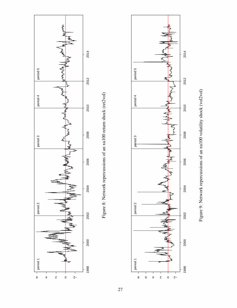
−20246

1998

2000

2002

2004

2006

2008

2010

2012

2014

perio

d 1

perio

d 2

perio

d 3

perio

d 4

perio

d 5

Figu

re8:

Net

wor

kre

perc

ussi

ons

ofan

xu10

0re

turn

shoc

k(r

et2v

ol)

−202468

1998

2000

2002

2004

2006

2008

2010

2012

2014

perio

d 1

perio

d 2

perio

d 3

perio

d 4

perio

d 5

Figu

re9:

Net

wor

kre

perc

ussi

ons

ofan

xu10

0vo

latil

itysh

ock

(vol

2vol

)

27

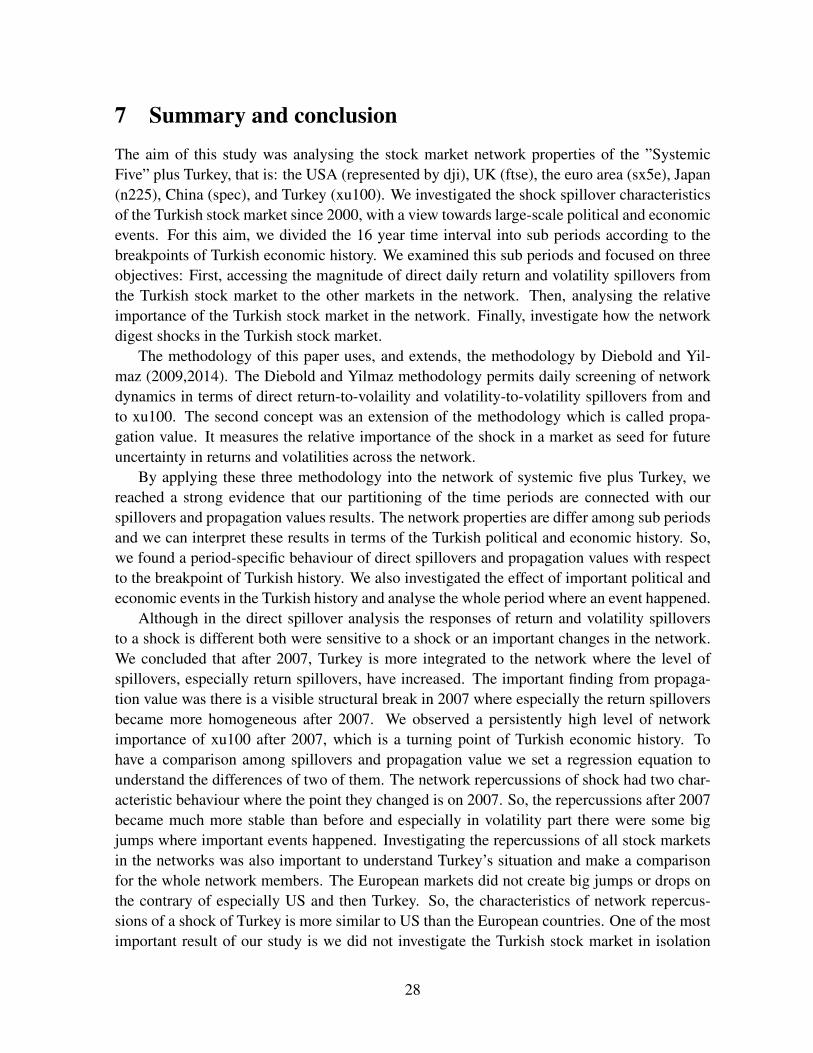
7 Summary and conclusionThe aim of this study was analysing the stock market network properties of the ”SystemicFive” plus Turkey, that is: the USA (represented by dji), UK (ftse), the euro area (sx5e), Japan(n225), China (spec), and Turkey (xu100). We investigated the shock spillover characteristicsof the Turkish stock market since 2000, with a view towards large-scale political and economicevents. For this aim, we divided the 16 year time interval into sub periods according to thebreakpoints of Turkish economic history. We examined this sub periods and focused on threeobjectives: First, accessing the magnitude of direct daily return and volatility spillovers fromthe Turkish stock market to the other markets in the network. Then, analysing the relativeimportance of the Turkish stock market in the network. Finally, investigate how the networkdigest shocks in the Turkish stock market.

The methodology of this paper uses, and extends, the methodology by Diebold and Yil-maz (2009,2014). The Diebold and Yilmaz methodology permits daily screening of networkdynamics in terms of direct return-to-volaility and volatility-to-volatility spillovers from andto xu100. The second concept was an extension of the methodology which is called propa-gation value. It measures the relative importance of the shock in a market as seed for futureuncertainty in returns and volatilities across the network.

By applying these three methodology into the network of systemic five plus Turkey, wereached a strong evidence that our partitioning of the time periods are connected with ourspillovers and propagation values results. The network properties are differ among sub periodsand we can interpret these results in terms of the Turkish political and economic history. So,we found a period-specific behaviour of direct spillovers and propagation values with respectto the breakpoint of Turkish history. We also investigated the effect of important political andeconomic events in the Turkish history and analyse the whole period where an event happened.

Although in the direct spillover analysis the responses of return and volatility spilloversto a shock is different both were sensitive to a shock or an important changes in the network.We concluded that after 2007, Turkey is more integrated to the network where the level ofspillovers, especially return spillovers, have increased. The important finding from propaga-tion value was there is a visible structural break in 2007 where especially the return spilloversbecame more homogeneous after 2007. We observed a persistently high level of networkimportance of xu100 after 2007, which is a turning point of Turkish economic history. Tohave a comparison among spillovers and propagation value we set a regression equation tounderstand the differences of two of them. The network repercussions of shock had two char-acteristic behaviour where the point they changed is on 2007. So, the repercussions after 2007became much more stable than before and especially in volatility part there were some bigjumps where important events happened. Investigating the repercussions of all stock marketsin the networks was also important to understand Turkey’s situation and make a comparisonfor the whole network members. The European markets did not create big jumps or drops onthe contrary of especially US and then Turkey. So, the characteristics of network repercus-sions of a shock of Turkey is more similar to US than the European countries. One of the mostimportant result of our study is we did not investigate the Turkish stock market in isolation

28

and comment on the Turkish political and economical events one by one, we approach to thegroup of stock markets as a network and analyse the characteristics of the network as a wholeand focus on the comparison of periods which was partitioned by considering the breakpointsof the Turkish economic history.

29

ReferencesAcemoglu, D., Ucer, M., 2015. The Ups and Downs of Turkish Growth, 2002-2015: Political

Dynamics, the European Union and the Institutional Slide. Nber Working Paper Series.

Andersen TG, Bollerslev T, Diebold FX, Ebens H (2001): The distribution of realized stockreturn volatility. Journal of Financial Economics 61, 43–76.

Akat, A.S., Yazgan, E. (2012): Observations on Turkey’s Recent Economic Performance.Atlantic Economic Journal Volume 41, Issue 1, pp 1-27.

Aloui R, Aissa MSB, Nguyen DK (2011): Global financial crisis, extreme interdependences,and contagion effects: The role of economic structure? Journal of Banking and Finance 35,130–141.

Barro, R., 1995. Inflation and economic growth. NBER Working Paper No: 5326.

Baur, D. (2003): Testing for contagion–Mean and volatility contagion. Journal of Multina-tional Financial Management 13, 405–422.

Bekiros, S.D. (2014): Contagion, decoupling and the spillover effects of the US financialcrisis: Evidence from the BRIC markets. International Review of Financial Analysis 33,58–69.

Bonacich P (1987): Power and centrality: a family of measures. American Journal of Sociol-ogy 92, 1170–1182.

Bonacich, P., Lloyd, P., 2001. Eigenvector-like measures of centrality for asymmetric relations.Social Networks 23, 191–201.

Baur, D. and Jung R.C. (2006). Return and volatility linkages between the US and the Germanstock market. Journal of International Money and Finance, 25, 598–613.

Bubak, V., Kocenda, E. and Zikes F. (2011). Volatility Transmission in Emerging EuropeanForeign Exchange Markets. Journal of Banking and Finance, 35(11), 2829–2841.

Chesney, M., Reshetar, G. and Karaman, M. (2010). The Impact of Terrorism on FinancialMarkets: An Empirical Study, SSRN Working Paper,

Christen, E., Fritz, O. and Streicher, G. (2015). Effects of the EU-Russia Economic Sanctionson Value Added and Employment in the European Union and Switzerland. Austrian Instituteof Economic Research, monograph, June 2015, 24 pages.

Choudhry, T., and Jayasekera, R. (2014). Returns and volatility spillover in the European bank-ing industry during global financial crisis: Flight to perceived quality or contagion? Inter-national Review of Financial Analysis, 36, 36–45.

30

Classens, S., and Forbes, K. (Eds.). International and Financial Contagion, (New York:Springer Science + Business Media, 2001)

Demiralay, S., and Bayraci, S. (2015). Central and Eastern European Stock Exchanges underStress: A Range-Based Volatility Spillover Framework. Czech Journal of Economics andFinance 65(5), 411-430.

Diebold FX, Yilmaz, K. (2009): Measuring Financial Asset Return and Volatility Spillovers,with Application to Global Equity Markets. Economic Journal 119, 158–171.

Diebold FX, Yilmaz, K. (2012): Better to give than to receive: Predictive directional measure-ment of volatility spillovers. International Journal of Forecasting 28, 57–66.

Diebold FX, Yilmaz, K. (2014): On The Network Topology of Variance Decompositions:Measuring The Connectedness of Financial Firms. Journal of Econometrics 182 (1), 119–134.

Dimpfl, T., and Jung, R.C. (2012). Financial market spillovers around the globe. Applied Fi-nancial Economics, 22, 45–57.

Dungey, M., Fry, R., Gonzalez-Hermosillo, B., Martin, V.L. (2005). Empirical Modelling ofContagion: a Review of Methodologies. Quantitative Finance 5, 9–24.

Engle, R.F., Ito, T., Lin, W. (1990). Meteor showers or heat waves? Heteroskedastic intra-dailyvolatility in the foreign exchange market. Econometrica 58, 525–542.

Fedorova, E., and Saleem, K. (2010). Volatility Spillovers between Stock and Currency Mar-kets: Evidence from Emerging Eastern Europe. Czech Journal of Economics and Finance60(6), 519–533.

Felipe, P.S., and Diranzo, F.C. (2006). Volatility transmission models: a survey. Revista Econo-mia Financiera 10(3), 32–81.

Garman MB, Klass MJ (1980): On the estimation of security price volatilities from historicaldata. Journal of Business, 53 (1), 67–78.

Gebka, B., and Serwa, D. (2007). Intra- and inter-regional spillovers between emerging capitalmarkets around the world. Research in International Business and Finance, 21, 203–221.

Golosnoy, V., Gribisch, B. and Liesenfeld, R. (2015). Intra-daily volatility spillovers in inter-national stock markets. Journal of International Money and Finance, 53, 95–114.

Gurkaynak, R., Sayek Boke, S. AKP doneminde Turkiye Ekonomisi Birikim dergisi, Aralik2012, Sayi 296

Hamao, Y., Masulis, R.W., and Ng, V. (1990). Correlations In Price Changes and VolatilityAcross International Stock Markets. The Review of Financial Studies 3(2), 281–307.

31

Harris, R.D.F., and Pisedtasalasai, A. (2006). Return and Volatility Spillovers Between Largeand Small Stocks in the UK. Journal of Business Finance and Accounting 33(9) & (10),15561571

International Monetary Fund (Ed.), (2008). 2008 Triennial Surveillance Review – OverviewPaper. International Monetary Fund, Washington D.C.

International Monetary Fund (Ed.), (2011a). 2011 Triennial Surveillance Review – OverviewPaper. International Monetary Fund, Washington D.C.

International Monetary Fund (Ed.) (2011b): 2011 Consolidated Spillover Report: ImplicationsFrom The Analysis of The Systemic-5. International Monetary Fund, Washington D.C.

International Monetary Fund (Ed.) (2012): 2012 Spillover Report – Background Papers. Inter-national Monetary Fund, Washington D.C.

Karolyi, G.A. (2003). Does International Financial Contagion Really Exist? InternationalFinance 6, 179–199.

King, M.A., Wadhwani, S. (1990). Transmission of volatility between stock markets. TheReview of Financial Studies 3(1), 5–33.

Lutkepohl, H., 2005. New Introduction to Multiple Time Series Analysis. Springer, New York.

Mandacı P.E., (2003). IMKBde Genel Secimler Oncesi ve Sonrasında Anormal Fiyat Hareket-leri, IMKB Dergisi, 7(27), 116.

Mutan, O.C., and Topcu A. (2009). Turkiye Hisse Senedi Piyasasının 1990-2009 TarihleriArasında Yasanan Beklenmedik Olaylara Tepkisi, Sermaye Piyasası Kurulu Arastırma Ra-poru.

Pericoli, M. and Sbracia, M. (2003). A Primer on Financial Contagion. Journal of EconomicSurveys 17(4), 571-608.

R Core Team (2015): R: A Language and Environment for Statistical Computing. R Founda-tion for Statistical Computing, Vienna, Austria.

Schmidbauer H, Rosch A, Uluceviz E (2013a): Information Propagation between Equity Mar-kets: the Case of BRICT. In: EcoMod Network (ed.), Proceedings of the InternationalConference on Policy Modeling EcoMod 2013, Prague, Czech Republic, July 1-3, 2013.Online, http://ecomod.net/conferences/ecomod2013?tab=downloads.

Schmidbauer H, Rosch A, Uluceviz E (2013b): Market Connectedness: Spillovers, Informa-tion Flow, and Relative Market Entropy. Koc University – TUSIAD Economic ResearchForum, Working Paper 1320 (October 2013).Online, http://eaf.ku.edu.tr/sites/eaf.ku.edu.tr/files/erf wp 1320.pdf

32

Susmel, R. and Engle, R.F. (1994). Hourly volatility spillovers between international equitymarkets. Journal of International Money and Finance 13(1), 3–25.

33

The Russian stock market duringthe Ukrainian crisis:

A Network Perspective∗

May 27, 2016

Abstract

The goal of the present paper is to investigate shock spillover characteristics of theRussian stock market during different rounds of sanctions imposed as a reaction to Rus-sia’s alleged role in the Ukrainian crisis.

We consider six stock markets, represented by their respective stock indices, namelyUSA (dji), UK (ftse), the euro area (sx5e), Japan (n225), China (ssec), and Russia (rts).Linking these markets together in a network on the basis of vector autoregressive pro-cesses, we can measure, among others: (i) direct daily return and volatility spilloversfrom rts to other market indices, (ii) daily propagation values quantifying the relative im-portance of the Russian stock market as a return or volatility shock propagator, (iii) theamount of network repercussions after a shock. The latter two are methodological inno-vations.

It turns out that distinct spillover patterns exist in different rounds of sanctions. Large-scale sanctions, beginning in July of 2014, left consequences of shocks from Russia lesspredictable. While these sanctions reduced the importance of the Russian stock market asa propagator of return shocks, they also increased its importance as a propagator of volatil-ity shocks, thus making the network more vulnerable with respect to volatility shocks fromthe Russian stock market. This is a form of backlash the sanctioning economies have beenfacing.

Key words: “Systemic Five”; Russian stock market; Ukrainian crisis; sanctions; returnspillovers; volatility spillovers; network dynamics; propagation value

∗The version of this research have been conditionally accepted on March 2016 and will be publish after aproper resubmission in the Czech Journal of Economics and Finance (CJEF). The paper is a joint work withHarald Schmidbauer, Angi Rosch and Erhan Uluceviz.

1

1 IntroductionRussia’s economy is of relatively moderate size in terms of aggregate figures. In 2013, Russia’sGDP was around 2.8% of the world GDP; the total value of Russia’s stock market in 2012 wasaround 1.5% of the world stock market value.1 Russia’s trading volume with the EU wasc. EUR 340 bn then2, and the EU had a GDP of c. EUR 13 500 bn.3 However, empiricalstudies have found evidence of strong dependence between Russia as one of the major rawmaterials exporter along with Brazil of the BRIC (Brazil, Russia, India, China) countries andthe US markets, and a significant increase of connectedness among BRIC equity markets andalso with equity markets in the developed world beginning in 2005 (see Aloui et al. (2011),Schmidbauer et al. (2013a)).

The recent sanctions against Russia, starting in March 2014, for its alleged role in theUkrainian crisis and annexation of Crimea4, may have contributed to structural changes ofRussian interconnectedness. Due to the sanctions, Russian companies faced difficulty rollingover debts from Western financial markets.5 The oil price drop from USD 100 (in June 2014)to USD 60 (in December 2014) further aggravated the situation, distorting the Russian budgetbalance and weakening the Russian economy significantly. As a result, companies’ demandfor dollars increased, followed by demand from Russian consumers. This initiated a vast rubledevaluation and forced the Central Bank of Russia to increase interest rates from 10.5% to17% in December 20146.

There are fears that the ruble’s devaluation could have adverse effects on the global econ-omy, as was experienced during the 1998 Russian crisis. Blanchard and Arezki from IMF alsowarn of the possible side effects of the Russian crisis7. On the other hand, there are viewssuggesting that the likelihood of such a contagious effect has decreased: “One major differ-

1Own calculations, based on data provided by the World Bank; see http://data.worldbank.org/data-catalog/GDP-ranking-table, http://data.worldbank.org/indicator/CM.MKT.TRAD.CD. Retrieved 2015-05-21.

2“European Union, Trade in goods with Russia”, released by the European Commission; available online athttp://trade.ec.europa.eu/doclib/docs/2006/september/tradoc 113440.pdf. Retrieved 2015-10-04

3See Eurostat database, http://ec.europa.eu/eurostat/tgm/refreshTableAction.do?tab=table&plugin=1&pcode=tec00001&language=en; data retrieved 2015-10-04.

4For EU sanctions, see http://europa.eu/newsroom/highlights/special-coverage/eu sanctions/index en.htm,and for US sanctions, see http://www.state.gov/e/eb/tfs/spi/ukrainerussia/, all retrieved 2015-05-27.

5“Western sanctions and rising debts are already strangling the Russian economy”, Forbes, 2014-08-28.Available online at http://www.forbes.com/sites/paulroderickgregory/2014/08/28/western-sanctions-and-rising-debts-are-already-strangling-the-russian-economy. Retrieved 2015-09-14.

6“Russian central bank raises interest rate to 17% to prevent ruble’s collapse”, The Guardian, 2014-12-15. Accessible online at http://www.theguardian.com/world/2014/dec/15/russia-interest-rate-rise-17pc-rouble-collapse-oil-price. Retrieved 2015-09-14)

7“Oil prices have plunged recently . . . One of the lessons from the Great Financial Crisis is that large changesin prices and exchange rates, and the implied increased uncertainty about the position of some firms and somecountries, can lead to increases in global risk aversion, with major implications for repricing of risk and forshifts in capital flows. This is all the more true when combined with other developments such as what ishappening in Russia. One cannot completely dismiss this tail risk.” The Guardian, 2014-12-22. Accessibleonline at http://www.inkl.com/news/trust-bank-becomes-first-financial-casualty-of-russia-s-currency-crisis. Re-trieved 2015-09-14.

2

ence between 1998 and today is that tough sanctions on Moscow have somewhat insulatedWestern investors from what’s ailing Russia. . . ” The sanctions regime has “reduced the riskfor financial contagion considerably. This is not 1998. You don’t have the same level of inter-connectedness,” comments Michael Levi, a senior fellow at the Council on Foreign Relations.(CNNMoney, 2014-12-17, retrieved 2015-05-27).

The goal of this study is to assess the influence of large-scale political and economic eventsand international sanctions on the importance of the Russian stock market as a news (or shock)propagator within a network of six stock markets, each represented by a stock index, namelyDow Jones Industrial Average (USA), FTSE (UK), Euro Stoxx 50 (euro area), Nikkei 225(Japan), SSE Composite (China), and RTS (Russia).8 The network is defined as a directedweighted graph with the stock indices as nodes and weights given by shock spillovers; see theexplanations below.

This perspective, which is not making physical spillover channels such as foreign tradeexplicit, has the advantage of using only data available on a daily basis. A network perspectivewas found useful for our purposes because events and sanctions won’t affect the Russian (orany other) market in isolation; markets are actually linked and a network perspective allows tostudy “event repercussions”.

The basic idea underlying the methodology used in this study is that the risk associatedwith investing in a market can be estimated by the variance of the error when forecasting afuture return on the market index. Vector autoregressive (VAR) models fitted to daily stockindex returns and volatilities can be used to derive the forecast error variance for each marketindex in the network, and to decompose this variance with respect to its origin: Which share ofstock market volatility is due to shocks in which other stock market? This approach provides aframework to discuss pairwise shock spillovers, arranged in a so-called spillover table, and wasproposed by Diebold and Yilmaz (2009, 2014). The spillover table is updated daily by fittingVAR models to a rolling window of return data. Schmidbauer et al. (2013b) discuss furtheraspects of spillover tables and show how to define the “propagation value” of a market, whichcan be interpreted as the relative importance of a market as news propagator and measures anaspect of centrality of the market in the network.

The methodology, as outlined, uses a VAR in daily returns; it can thus assess daily return-to-volatility spillovers (for simplicity, called the ret2vol case in the following), that is, it per-mits to trace the network consequences (in terms of return volatility) of a return shock to amarket. Again, following Diebold and Yilmaz (2009), it is also possible to fit VAR models todaily return volatilities (instead of returns themselves), and proceed as before; this approachcan quantify volatility-to-volatility spillovers (the vol2vol case), that is, the network conse-quences (in terms of volatility risk) of a volatility shock to a market. Both concepts — ret2volas well as vol2vol — are used in the present study.

More specifically, this study focuses on the following objectives:

1. Assess the magnitude of direct daily ret2vol and vol2vol spillovers from the Russianstock market (that is, from rts) to other markets (to other nodes) in the network. This

8The former five are dubbed the “Systemic Five” economies in IMF spillover reports IMF (2011, 2012).

3

perspective focuses on one-time spillovers; it does not take repercussions of a shock inthe network into account. This task can be achieved using raw spillover tables.

2. Assess the relative importance of the Russian stock market as a return or volatility shockpropagator in the network. This perspective complements objective 1 insofar as it ac-counts for aftereffects of a one-time shock. This can be achieved using daily propagationvalues.

3. Provide insight into the network repercussions of an initial shock, that is, into how thenetwork ultimately digests shocks in the Russian stock market. This amounts to a com-parison of network importance (objective 2) and direct spillovers (objective 1). This canbe achieved by regressing propagation values on direct spillovers.

We are, in particular, interested in detecting differences between different rounds of thesanctions with respect to these characteristics, and in assessing the impact of political andeconomic events on them. Consequently, this paper continues with a brief account of thesequence of events and of the international sanctions in connection with the Ukrainian crisisthey entailed, given in Section 2. A glance is thrown at the empirical data (essentially, dailystock index quotations from six markets) used in the present study in Section 3. In Section 4,we first review the theory underlying the spillover perspective (objective 1 above) and thenintroduce further methodology to discuss objectives 2 and 3. The subsequent sections reportand discuss empirical results concerning objective 1 (Section 5), objective 2 (Section 6), andobjective 3 (Section 7). Section 8 summarizes and concludes the paper. — All computationswere carried out with scripts written in R (2015).

2 Events and sanctions in connection with the Ukrainian cri-sis

2.1 Events prior to sanctionsThe Ukrainian crisis began in the night of 2013-11-21 with waves of calm protests in Kievagainst the then-president of Ukraine who, fancying the prospect of a Russian-led alliance,had suspended an association agreement with the European Union.9

On 2014-01-29, Russia “raised the economic pressure on Ukraine”, in reversal of its decla-ration of intention made on an EU-Russia summit the previous day, announcing the suspensionof its financial aid commitments to Ukraine, which would be fulfilled “only when we knowwhat economic policies the new government will implement, who will be working there, andwhat rules they will follow”.10

9“Kiev protesters gather, EU dangles aid promise”, Reuters, 2013-12-12; available online athttp://www.reuters.com/article/2013/12/12/us-ukraine-idUSBRE9BA04420131212. Retrieved 2015-09-15.

10“Russia Defers Aid to Ukraine, and Unrest Persists”, The New York Times, 2014-01-29; available online athttp://www.nytimes.com/2014/01/30/world/europe/ukraine-protests.html? r=0. Retrieved 2015-10-04.

4

The anti-governmental demonstrations in Ukraine culminated in violent clashes with thepolice on 2014-02-18, known as the “2014 Ukrainian revolution”, which led to the oustingof the Ukrainian president two days later and the installation of an interim government.11 Inthe aftermath, pro-Russian and anti-revolution protests and activism gripped Crimea and partsof eastern and southern Ukraine, while the Olympic Games (2014-02-07 through 2014-02-23) in nearby Sochi, Russia, were about to end. On 2014-02-27, the Supreme Council ofCrimea was taken over by unidentified pro-Russian gunmen12, leading to the installation ofa pro-Russian government in Crimea declaring Crimea’s independence. On 2014-03-01, theRussian president Vladimir Putin had officially requested (and was granted) parliamentaryauthorization to “use force in Ukraine to protect Russian interests”.13

2.2 Implementation of international sanctionsIn retrospect, international sanctions imposed so far in connection with the Ukrainian crisiscan be grouped into three rounds:

• First round, starting 2014-03-06: The first round of sanctions essentially involves travelbans and asset freezes targeting individuals and entities allegedly instrumental for ac-tions undermining Ukraine’s sovereignty.

On 2014-03-06, through executive order14, US president Barack Obama stated thatevents in the Crimean region “. . . constitute an unusual and extraordinary threat to thenational security and foreign policy of the United States. . . ” and ordered the blockingof property of “certain persons contributing to the situation in Ukraine”.

A secession referendum, internationally disputed as illegitimate, was held on 2014-03-16, resulting in the Russian annexation of Crimea on 2014-03-18.15 The involvement ofincognito Russian armed forces has been admitted by the Russian president only later,on 2014-04-17.16,17

11“Ukraine crisis: Timeline”, BBC news, 2014-11-13; available online at http://www.bbc.com/news/world-middle-east-26248275. Retrieved 2015-09-15.

12“How the separatists delivered Crimea to Moscow”, Reuters, 2014-03-13; available online atn.reuters.com/article/2014/03/13/ukraine-crisis-russia-aksyonov-idINL6N0M93AH20140313. Retrieved 2015-09-15.

13“Ukraine crisis: Timeline”, BBC news, 2014-11-13; available online at http://www.bbc.com/news/world-middle-east-26248275. Retrieved 2015-09-15.

14“Executive Order – Blocking Property of Certain Persons Contributing to the Situation in Ukraine”, released2014-03-06 by the White House Press Secretary; available online at https://www.whitehouse.gov/the-press-office/2014/03/06/executive-order-blocking-property-certain-persons-contributing-situation. Retrieved 2015-09-14.

15“Putin signs laws on reunification of Republic of Crimea and Sevastopol with Russia”, TASS, 2014-03-21;available online at http://tass.ru/en/russia/724785. Retrieved 2015-09-15.

16“Vladimir Putin admits for first time Russian troops took over Crimea, refuses to rule out interventionin Donetsk”, National Post, 2014-04-17; available online at http://news.nationalpost.com/news/world/vladimir-putin-admits-for-first-time-russian-troops-took-over-crimea-refuses-to-rule-out-intervention-in-donetsk. Re-trieved 2015-09-15.

17“Direct line with Vladimir Putin” (in Russian), released on 2014-04-17 by the Kremlin; available online at

5

On 2014-03-17, the US extended its list of persons targeted, and also the EU declaredsanctions specifically targeted against certain individuals18,19. Furthermore, Canada20,Japan21 and Australia22 also imposed sanctions against Russia in the spirit of sanctionsof the US and the EU.

• Second round, starting 2014-04-28: The second round of sanctions by the US “. . . [was]taken in close coordination with the EU.”23 In the second round, in addition to thefirst-round sanctions, bans on business transactions of several Russian government of-ficials and entities (defense, energy companies and banks) were imposed.24 The EUextended the list of individuals targeted with a travel ban and a freeze of their assetswithin the EU.25

• Third round, starting 2014-07-16: The third round of sanctions, building upon previousrounds, is marked with the announcement of the US Treasury to take a “broad-basedpackage” of sanctions against certain major Russian financial institutions, energy firms,defense technology entities, as well as on “those undermining Ukraine’s sovereigntyor misappropriating Ukrainian property”.26 These sanctions pronouncedly aimed to

http://kremlin.ru/events/president/news/20796. Retrieved 2015-09-15.18“Executive Order – Blocking Property of Additional Persons Contributing to the Situation in Ukraine”,

released 2014-03-17 by the White House Press Secretary; available online at https://www.whitehouse.gov/the-press-office/2014/03/17/executive-order-blocking-property-additional-persons-contributing-situat. Retrieved2015-09-14.

19“Council decision 2014/145/CFSP of 17 March 2014 concerning restrictive measures in re-spect of actions undermining or threatening the territorial integrity, sovereignty and independence ofUkraine”, released 2014-03-17 by the Council of the European Union; available online at http://eur-lex.europa.eu/LexUriServ/LexUriServ.do?uri=OJ:L:2014:078:0016:0021:EN:PDF. Retrieved 2015-09-14.

20“Canadian Sanctions Related to Russia”, released 2014-03-17 by the Government of Canada; availableonline at http://www.international.gc.ca/sanctions/countries-pays/russia-russie.aspx?lang=eng. Retrieved 2015-09-14.

21“Statement by the Minister for Foreign Affairs of Japan on the Sanctions against Russia over the situationin Ukraine”, released 2014-04-29; available online at http://www.mofa.go.jp/press/release/press4e 000281.html.Retrieved 2015-09-14.

22“Sanctions regimes – Russia”, released 2014-03-19 by the Australian Government; available onlineat https://dfat.gov.au/international-relations/security/sanctions/sanctions-regimes/Pages/russia.aspx. Retrieved2015-09-14.

23“Statement Of Treasury Secretary Jacob J. Lew”, released 2014-04-28; available online athttp://www.treasury.gov/press-center/press-releases/Pages/jl2368.aspx. Retrieved 2015-09-14.

24For further details, see “Ukraine and Russia Sanctions”, available online athttp://www.state.gov/e/eb/tfs/spi/ukrainerussia/, issued by the US Department of State. Retrieved 2015-09-14.

25“EU strengthens sanctions against actions undermining Ukraine’s territorial in-tegrity”, released 2014-04-28 by the Council of the European Union; available online athttps://www.consilium.europa.eu/uedocs/cms Data/docs/pressdata/EN/foraff/142411.pdf. Retrieved 2015-08-22.

26“Announcement of treasury sanctions on entities within the financial services and energy sectors of Rus-sia, against arms or related materiel entities, and those undermining Ukraine’s sovereignty”, released 2014-07-16 by the US Department of the Treasury; available online at http://www.treasury.gov/press-center/press-releases/Pages/jl2572.aspx. Retrieved 2015-09-14.

6

“. . . [increase] the cost of economic isolation for key Russian firms that value their ac-cess to medium- and long-term US sources of financing. By designating firms in thearms or related materiel sector, Treasury has cut these firms off from the U.S. financialsystem and the U.S. economy”.

The downing of a Malaysian airplane over separatist-held territory in Ukraine on 2014-07-17 exacerbated the confrontation between Russia and Western countries dramatically.On 2014-07-22, the EU agreed to draft a new list of Russian individuals and entities to betargeted by travel bans and asset freezes. At the same time, the EU threatened to quicklypass on to extensive sectoral “phase three sanctions” if Russia continued its alleged sup-port of separatists, believed to have shot down the plane, and refused to cooperate withan international inquiry.27 On 2014-07-29, the EU decided that Russia had not compliedwith these conditions and agreed on sweeping economic sanctions, targeting “economiccooperation and exchanges with Russia”, to come into force on 2014-07-31.28 Thesesanctions “limited access to EU capital markets for Russian State-owned financial insti-tutions”, established an arms embargo and an export ban for sensitive technology andequipment for the oil industry. The US joined the EU with new measures, in particularcutting off three prominent Russian banks from the US economy.29 Tougher sanctionswere also announced by Canada (2014-07-24), Japan (2014-08-05), Norway (2014-08-12), Switzerland (2014-08-14), and Australia (2014-09-01). Alleged evidence of Rus-sia’s involvement in separatists’ fights led the EU to expand and strengthen sanctionseven further on 2014-09-1230, aligned with the US31, while Japan implemented strictersanctions on 2014-09-24. However, reports like that of Russian tanks “crossing bor-der” into eastern Ukraine on 2014-11-07, a few days after the separatists’ proposal to

27“E.U. imposes new sanctions on Russian officials, stops short of tougher penalties”, The Washington Post,2014-07-22; available online at https://www.washingtonpost.com/world/europe/eu-foreign-ministers-confer-on-tougher-sanctions-against-russia/2014/07/22/05e1d794-1197-11e4-8936-26932bcfd6ed story.html. Retrieved2015-09-30.

28“Statement by the President of the European Council Herman Van Rompuy and the President ofthe European Commission in the name of the European Union on the agreed additional restrictive mea-sures against Russia”, released 2014-07-29; available online at http://europa.eu/newsroom/highlights/special-coverage/eu sanctions/index en.htm#6. Retrieved 2015-09-30.“Council regulation (EU) No 833/2014 of 31 July 2014 concerning restrictive measures in view of Russia’sactions destabilising the situation in Ukraine”, released 2014-07-31 by the Council of the European Union; avail-able online at http://eur-lex.europa.eu/legal-content/EN/TXT/PDF/?uri=OJ:JOL 2014 229 R 0001&from=EN.Retrieved 2015-09-14.

29“EU and US impose sweeping economic sanctions on Russia”, The Guardian, 2014-07-29; available onlineat http://www.theguardian.com/world/2014/jul/29/economic-sanctions-russia-eu-governments. Retrieved 2015-09-30.

30“Reinforced restrictive measures against Russia”, released 2014-09-11 by the Council of the EuropeanUnion; available online at http://europa.eu/newsroom/highlights/special-coverage/eu sanctions/index en.htm#6.Retrieved 2015-09-30.

31“Obama says U.S. to outline new Russia sanctions on Friday”, Reuters, 2014-09-11; available online athttp://www.reuters.com/article/2014/09/11/us-ukraine-crisis-obama-sanctions-idUSKBN0H620I20140911. Re-trieved 2015-09-30.

7

establish a “People’s Republic”, officially “respected” by Russia32, continued fuelingconcerns of “Russia’s aggression and direct involvement in destabilising Ukraine”.

Bans on investments in Crimea were first implemented by the EU on 2014-12-18, andthe following day by the US.33,34 In view of the escalation of violence in Ukraine, theEU Council, on its 2015-01-29 summit in Minsk, decided to extend existing restrictivemeasures until September 2015, adding to the list of targeted individuals and entities on2015-02-16.35,36 Canada followed suit on 2015-02-18. At their 2015-06-07/08 summit,the G7 leaders declared their commitment to uphold sanctions, the duration of which“should be clearly linked to Russia’s complete implementation of the Minsk agreementsand respect for Ukraine’s sovereignty” and to “take further restrictive measures in orderto increase cost on Russia should its actions so require”.37

2.3 Further events in the wake of sanctionsEvents with an economic backgroundIn response to the international sanctions, Russia imposed bans on food imports from thesanctioning countries on 2014-08-06.38

In December 2014, a vast devaluation seized the already weak ruble. On 2014-12-02,Russia acknowledged that it “will fall into recession next year, battered by the combinationof Western sanctions and a plunge in the price of its oil exports”.39 On 2014-12-09, minglingwith the World Bank’s revision of its economic outlook for Russia40, bad news also came from

32“Ukraine crisis: Tanks ’cross border’ from Russia”, BBC News 2014-11-07; available online athttp://www.bbc.com/news/world-europe-29952505. Retrieved 2015-10-11.

33“EU bans investment in Crimea, targets oil sector, cruises”, Reuters, 2014-12-18; available online athttp://www.reuters.com/article/2014/12/18/us-ukraine-crisis-eu-idUSKBN0JW18020141218. Retrieved 2015-10-07.

34“US slaps trade ban on Crimea over Russia “occupation””, The Telegraph, 2014-12-20; availableonline at http://www.telegraph.co.uk/news/worldnews/europe/ukraine/11305372/US-slaps-trade-ban-on-Crimea-over-Russia-occupation.html. Retrieved 2015-10-07.

35Press release by the Foreign Affairs Council, 29/01/2015; available online athttp://www.consilium.europa.eu/en/meetings/fac/2015/01/29/. Retrieved 2015-10-07.

36“New EU Sanctions Hit 2 Russian Deputy DMs”, Defense News, 2015-02-16; available on-line at http://www.defensenews.com/story/defense/international/europe/2015/02/16/official-new-eu-sanctions-hit-two-russian-deputy-defence-ministers/23527227/. Retrieved 2015-10-07.

37“Leaders’ Declaration G7 Summit”, released on 2015-06-08; available online athttps://www.g7germany.de/Content/DE/ Anlagen/G8 G20/2015-06-08-g7-abschluss-eng.html?nn=1281552.Retrieved 2015-10-07.

38“Russia hits West with food import ban in sanctions row”, released 2014-08-07; available online athttp://www.bbc.com/news/world-europe-28687172. Retrieved 2015-08-22.

39“Russia warns of recession next year”, The Washington Times, 2014-12-02; available on-line at http://www.washingtontimes.com/news/2014/dec/2/russia-warns-recession-next-year-ruble-falls-recor/?page=all. Retrieved 2015-10-11.

40“World Bank Revises Its Growth Projections for Russia for 2015 and 2016”, released 2014-12-09 bythe World Bank; available online at http://www.worldbank.org/en/news/press-release/2014/12/08/world-bank-revises-its-growth-projections-for-russia-for-2015-and-2016. Retrieved 2015-10-12.

8

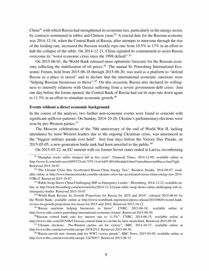
China41 with which Russia had strengthened its economic ties, particularly in the energy sector,by contracts nominated in rubles and Chinese yuan.42 A crucial date for the Russian economywas 2014-12-16, when the Central Bank of Russia, after attempts to intervene through the riseof the lending rate, increased the Russian weekly repo rate from 10.5% to 17% in an effort tohalt the collapse of the ruble. On 2014-12-21, China signaled its commitment to assist Russiaovercome its “worst economic crisis since the 1998 default”.43

On 2015-06-01, the World Bank released more optimistic forecasts for the Russian econ-omy reflecting the stabilization of oil prices.44 The annual St. Petersburg International Eco-nomic Forum, held from 2015-06-18 through 2015-06-20, was used as a platform to “defendRussia as a place to invest” and to declare that the international economic sanctions were“helping Russian businesses to thrive”.45 On this occasion, Russia also declared its willing-ness to intensify relations with Greece suffering from a severe government-debt crisis. Justone day before the forum opened, the Central Bank of Russia had cut its repo rate down againto 11.5% in an effort to stimulate economic growth.46

Events without a direct economic backgroundIn the course of the analysis, two further non-economic events were found to coincide withsignificant spillover patterns: On Sunday, 2014-10-26, Ukraine’s parliamentary elections werewon by pro-Western parties.47

The Moscow celebrations of the 70th anniversary of the end of World War II, lackingattendance by most Western leaders due to the ongoing Ukrainian crisis, was announced asthe “biggest military parade ever held”. Just four days before the Victory Day Parade, on2015-05-05, a new-generation battle tank had been unveiled to the public.48

On 2015-05-22, an EU summit with six former Soviet states ended in Latvia, reconfirming

41“Shanghai stocks suffer sharpest fall in five years”, Financial Times, 2014-12-09; available online athttp://www.ft.com/intl/cms/s/0/95372ce6-7f79-11e4-b4f5-00144feabdc0.html?siteedition=intl#axzz3nst55gjh.Retrieved 2015-10-07.

42“The Ukraine Crisis Has Accelerated Russia-China Energy Ties”, Business Insider, 2014-09-07; avail-able online at http://www.businessinsider.com/the-ukraine-crisis-has-accelerated-russia-china-energy-ties-2014-9?IR=T. Retrieved 2015-10-07.

43“Ruble Swap Shows China Challenging IMF as Emergency Lender”, Bloomberg, 2014-12-22; available on-line at http://www.bloomberg.com/news/articles/2014-12-22/yuan-ruble-swap-shows-china-challenging-imf-as-emergency-lender. Retrieved 2015-10-07.

44“World Bank Revises Its Growth Projections for Russia for 2015 and 2016”, released 2015-06-01 bythe World Bank; available online at http://www.worldbank.org/en/news/press-release/2015/06/01/world-bank-revises-its-growth-projections-for-russia-for-2015-and-2016. Retrieved 2015-10-12.

45“Russia sanctions helping businesses to thrive”, CNBC, 2015-06-18; available online athttp://www.cnbc.com/st-petersburg-international-economic-forum/. Retrieved 2015-09-30.

46Russian central bank cuts key interest rate to 11.5%”, CNBC, 2014-06-15; available online athttp://www.cnbc.com/2015/06/15/russia-central-bank-to-cut-but-by-how-much.html. Retrieved 2015-09-30.

47“Ukraine elections: Pro-Western parties set for victory”, BBC, 2014-10-27; available online athttp://www.bbc.com/news/world-europe-29782513. Retrieved 2015-09-30.

48“Russia unveils new Armata tank for WW2 victory parade”, BBC News, 2015-05-05; available online athttp://www.bbc.com/news/world-europe-32478937. Retrieved 2015-09-15.

9

period remarks begins ends mean sd0 before 2014 1998-07-20 2013-12-31 0.079 2.4181 2014, before sanctions 2014-01-01 2014-03-05 −0.406 2.2852 first round of sanctions 2014-03-06 2014-04-25 −0.127 2.0673 second round of sanctions 2014-04-28 2014-07-15 0.341 1.3904 third round of sanctions 2014-07-16 2014-12-15 −0.558 2.0095 after increase in repo rate 2014-12-16 2015-07-06 0.199 2.840

Table 1: Periods, daily average returns and standard deviations of rts

the determination and importance the EU attaches to its “Eastern Partnership”.49 The fol-lowing Sunday, 2015-05-24, Russia passed a bill which allowed the prosecution of foreignnon-governmental organizations labeled as “undesirable”.50 A “blacklist” of European offi-cials with entry ban was revealed a few days later, on 2015-05-2951 — amid concerns that“Russia masses heavy firepower” on its border to Ukraine.52

2.4 Partitioning the time periodThe goal of the sanctions was to impose costs on the Russian economy. For our purposes, thisleads to the partitioning of the time period under consideration shown in Table 1.53

It should be emphasized that this partitioning is apriori in the sense that network properties(reported and analyzed in Sections 5, 6, and 7) are not used in defining sub-periods. At thispoint, our working hypothesis is that network properties are different in different periods.

3 DataThe empirical starting point of the present study consists of daily closing quotations of theRussian stock index (rts) and the five stock indices representing stock markets in the “SystemicFive” countries: Dow Jones Industrial Average (USA; dji), FTSE (UK; ftse), Euro Stoxx 50(euro area; sx5e), Nikkei 225 (Japan; n225), and SSE Composite (China; ssec). The series

49“Eastern Partnership summit, Riga, 21-22/05/2015”, released by the European Council, 2014-05-22;available online at http://www.consilium.europa.eu/en/meetings/international-summit/2015/05/21-22/. Retrieved2015-09-30.

50“Russia’s Putin signs law against “undesirable” NGOs”, BBC, 2015-05-24; available online athttp://www.bbc.com/news/world-europe-32860526. Retrieved 2015-09-30.

51“Russia releases 89-name EU travel blacklist”, Yahoo! News, 2015-05-29; available online athttp://news.yahoo.com/russia-issues-blacklist-bars-eu-politicians-dutch-pm-164848974.html. Retrieved 2015-10-07.

52“Exclusive: Russia masses heavy firepower on border with Ukraine — witness”, Reuters,2015-05-27; available online at http://www.reuters.com/article/2015/05/27/us-ukraine-crisis-russia-military-idUSKBN0OC2K820150527. Retrieved 2015-10-08.

531998-07-20 is the first day for which all measures reported below were available.

10

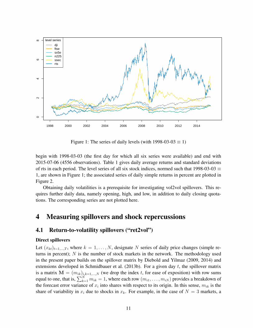
02

46

8 level series

djiftsesx5en225ssecrts

1998 2000 2002 2004 2006 2008 2010 2012 2014

Figure 1: The series of daily levels (with 1998-03-03 ≡ 1)

begin with 1998-03-03 (the first day for which all six series were available) and end with2015-07-06 (4556 observations). Table 1 gives daily average returns and standard deviationsof rts in each period. The level series of all six stock indices, normed such that 1998-03-03 ≡1, are shown in Figure 1; the associated series of daily simple returns in percent are plotted inFigure 2.

Obtaining daily volatilities is a prerequisite for investigating vol2vol spillovers. This re-quires further daily data, namely opening, high, and low, in addition to daily closing quota-tions. The corresponding series are not plotted here.

4 Measuring spillovers and shock repercussions

4.1 Return-to-volatility spillovers (“ret2vol”)Direct spilloversLet (xkt)t=1,...,T , where k = 1, . . . , N , designate N series of daily price changes (simple re-turns in percent); N is the number of stock markets in the network. The methodology usedin the present paper builds on the spillover matrix by Diebold and Yilmaz (2009, 2014) andextensions developed in Schmidbauer et al. (2013b). For a given day t, the spillover matrixis a matrix M = (mik)i,k=1,...,N (we drop the index t, for ease of exposition) with row sumsequal to one, that is,

∑Nk=1mik = 1, where each row (mi1, . . . ,miN) provides a breakdown of

the forecast error variance of xi into shares with respect to its origin. In this sense, mik is theshare of variability in xi due to shocks in xk. For example, in the case of N = 3 markets, a

11

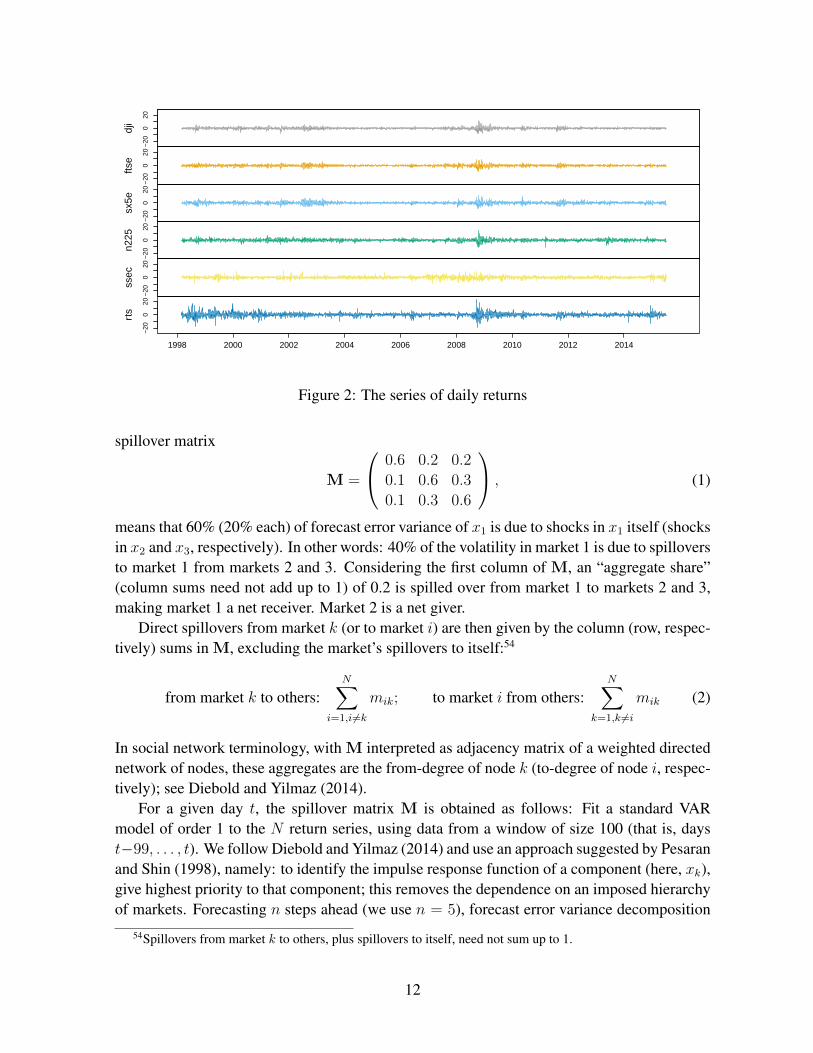
−20

020

dji

−20

020

ftse

−20

020

sx5e

−20

020

n225

−20

020

ssec

−20

020

rts

1998 2000 2002 2004 2006 2008 2010 2012 2014

Figure 2: The series of daily returns

spillover matrix

M =

0.6 0.2 0.2

0.1 0.6 0.3

0.1 0.3 0.6

, (1)

means that 60% (20% each) of forecast error variance of x1 is due to shocks in x1 itself (shocksin x2 and x3, respectively). In other words: 40% of the volatility in market 1 is due to spilloversto market 1 from markets 2 and 3. Considering the first column of M, an “aggregate share”(column sums need not add up to 1) of 0.2 is spilled over from market 1 to markets 2 and 3,making market 1 a net receiver. Market 2 is a net giver.

Direct spillovers from market k (or to market i) are then given by the column (row, respec-tively) sums in M, excluding the market’s spillovers to itself:54

from market k to others:N∑

i=1,i 6=k

mik; to market i from others:N∑

k=1,k 6=i

mik (2)

In social network terminology, with M interpreted as adjacency matrix of a weighted directednetwork of nodes, these aggregates are the from-degree of node k (to-degree of node i, respec-tively); see Diebold and Yilmaz (2014).

For a given day t, the spillover matrix M is obtained as follows: Fit a standard VARmodel of order 1 to the N return series, using data from a window of size 100 (that is, dayst−99, . . . , t). We follow Diebold and Yilmaz (2014) and use an approach suggested by Pesaranand Shin (1998), namely: to identify the impulse response function of a component (here, xk),give highest priority to that component; this removes the dependence on an imposed hierarchyof markets. Forecasting n steps ahead (we use n = 5), forecast error variance decomposition

54Spillovers from market k to others, plus spillovers to itself, need not sum up to 1.

12

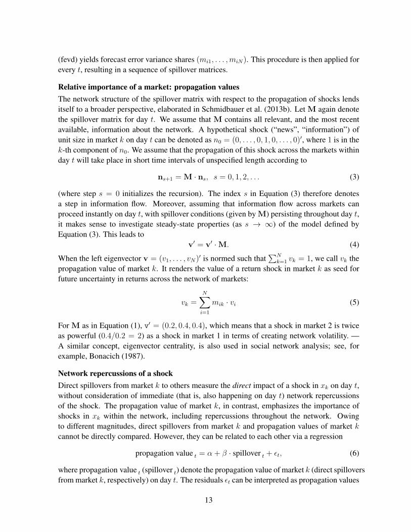
(fevd) yields forecast error variance shares (mi1, . . . ,miN). This procedure is then applied forevery t, resulting in a sequence of spillover matrices.

Relative importance of a market: propagation valuesThe network structure of the spillover matrix with respect to the propagation of shocks lendsitself to a broader perspective, elaborated in Schmidbauer et al. (2013b). Let M again denotethe spillover matrix for day t. We assume that M contains all relevant, and the most recentavailable, information about the network. A hypothetical shock (“news”, “information”) ofunit size in market k on day t can be denoted as n0 = (0, . . . , 0, 1, 0, . . . , 0)′, where 1 is in thek-th component of n0. We assume that the propagation of this shock across the markets withinday t will take place in short time intervals of unspecified length according to

ns+1 = M · ns, s = 0, 1, 2, . . . (3)

(where step s = 0 initializes the recursion). The index s in Equation (3) therefore denotesa step in information flow. Moreover, assuming that information flow across markets canproceed instantly on day t, with spillover conditions (given by M) persisting throughout day t,it makes sense to investigate steady-state properties (as s → ∞) of the model defined byEquation (3). This leads to

v′ = v′ ·M. (4)

When the left eigenvector v = (v1, . . . , vN)′ is normed such that

∑Nk=1 vk = 1, we call vk the

propagation value of market k. It renders the value of a return shock in market k as seed forfuture uncertainty in returns across the network of markets:

vk =N∑i=1

mik · vi (5)

For M as in Equation (1), v′ = (0.2, 0.4, 0.4), which means that a shock in market 2 is twiceas powerful (0.4/0.2 = 2) as a shock in market 1 in terms of creating network volatility. —A similar concept, eigenvector centrality, is also used in social network analysis; see, forexample, Bonacich (1987).

Network repercussions of a shockDirect spillovers from market k to others measure the direct impact of a shock in xk on day t,without consideration of immediate (that is, also happening on day t) network repercussionsof the shock. The propagation value of market k, in contrast, emphasizes the importance ofshocks in xk within the network, including repercussions throughout the network. Owingto different magnitudes, direct spillovers from market k and propagation values of market kcannot be directly compared. However, they can be related to each other via a regression

propagation value t = α + β · spillover t + εt, (6)

where propagation value t (spillover t) denote the propagation value of market k (direct spilloversfrom market k, respectively) on day t. The residuals εt can be interpreted as propagation values

13

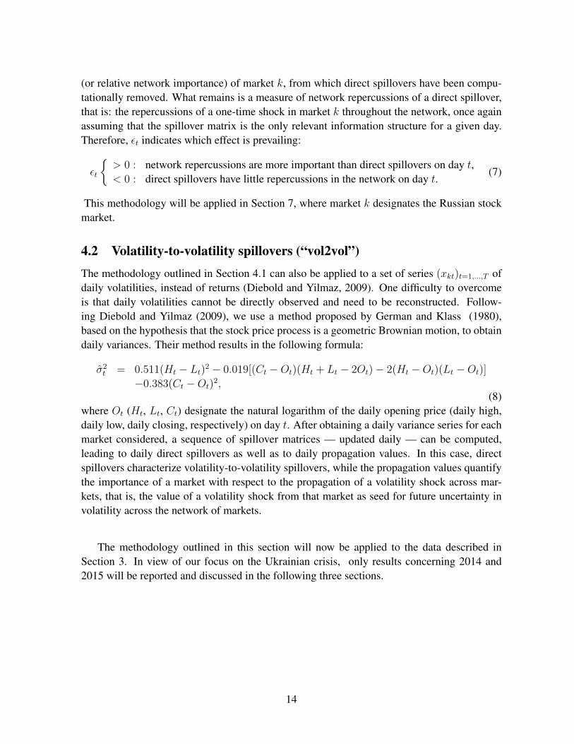
(or relative network importance) of market k, from which direct spillovers have been compu-tationally removed. What remains is a measure of network repercussions of a direct spillover,that is: the repercussions of a one-time shock in market k throughout the network, once againassuming that the spillover matrix is the only relevant information structure for a given day.Therefore, εt indicates which effect is prevailing:

εt

{> 0 : network repercussions are more important than direct spillovers on day t,< 0 : direct spillovers have little repercussions in the network on day t.

(7)

This methodology will be applied in Section 7, where market k designates the Russian stockmarket.

4.2 Volatility-to-volatility spillovers (“vol2vol”)The methodology outlined in Section 4.1 can also be applied to a set of series (xkt)t=1,...,T ofdaily volatilities, instead of returns (Diebold and Yilmaz, 2009). One difficulty to overcomeis that daily volatilities cannot be directly observed and need to be reconstructed. Follow-ing Diebold and Yilmaz (2009), we use a method proposed by German and Klass (1980),based on the hypothesis that the stock price process is a geometric Brownian motion, to obtaindaily variances. Their method results in the following formula:

σ2t = 0.511(Ht − Lt)

2 − 0.019[(Ct −Ot)(Ht + Lt − 2Ot)− 2(Ht −Ot)(Lt −Ot)]

−0.383(Ct −Ot)2,

(8)where Ot (Ht, Lt, Ct) designate the natural logarithm of the daily opening price (daily high,daily low, daily closing, respectively) on day t. After obtaining a daily variance series for eachmarket considered, a sequence of spillover matrices — updated daily — can be computed,leading to daily direct spillovers as well as to daily propagation values. In this case, directspillovers characterize volatility-to-volatility spillovers, while the propagation values quantifythe importance of a market with respect to the propagation of a volatility shock across mar-kets, that is, the value of a volatility shock from that market as seed for future uncertainty involatility across the network of markets.

The methodology outlined in this section will now be applied to the data described inSection 3. In view of our focus on the Ukrainian crisis, only results concerning 2014 and2015 will be reported and discussed in the following three sections.

14

5 Direct spillovers from and to rtsThis section reports the first part of spillover characteristics of the Russian stock market,namely direct return and volatility spillovers, without considering potential aftereffects of ashock. The subsequent Sections 6 and 7 will give more detailed interpretations, using themethodological innovations (propagation values and network repercussions) introduced inSections 4.1 and 4.2. Particular attention will be given to the following periods and events(cf. Section 2):

• End of period 1 / beginning of period 2 (roughly, late January 2014 – early March 2014):Russia increased the economic pressure on Ukraine. The Olympic Games began inSochi, Russia. In the run-up to the first round of sanctions, Russia’s president wasgranted parliamentary authorization to “use force in Ukraine to protect Russian inter-ests”.

• Beginning of period 4 (roughly, 2nd half of July 2014):The third round of sanctions entailed extensive sectoral measures targeting Russia’seconomy on a broad base, while the first and second rounds had imposed travel bansand asset freezes on Russian individuals and entities. The US were the first to take thisstep. The downing of the Malaysian airplane worsened the relations between Russia andWestern countries to the effect that the EU joined, and tightened, economic sanctionstwo weeks later.

• End of period 4 / beginning of period 5 (roughly, late October 2014 – December 2014):Ukraine’s parliamentary elections were won by pro-Western parties. Falling crude oilprices further aggravated Russia’s economic situation, leading Russia to acknowledgethat it was heading towards a recession. A ruble crisis was triggered, which finally madethe Central Bank of Russia increase the weekly repo rate significantly.

• Later part of period 5 (roughly, May – June 2015):Russia’s Victory Day Parade in early May was received in the Western world as a show-off of Russian military strength. Later this month, reports that Russia masses militarypower on its border to Ukraine further strained relations between Russia and the EU. TheSt. Petersburg International Economic Forum held in mid-June was used as a platformto advertise businesses and investments in Russia.

5.1 The case return-to-volatility (ret2vol)The daily series of direct return spillovers from rts to others and from others to rts are displayedin Figure 3 for the period from January 2014 through July 2015. Return spillovers to rtshave always been higher than return spillovers from rts after the first round of sanctions wasimposed. This was also true for a high share of earlier days, so that the Russian market hasbeen a net receiver of return shocks — at least when potential aftereffects of shocks in the

15

network are ignored; cf. Table 2. Periods 2 and 3 can be jointly characterized as havingpersistently elevated levels of return spillovers; the latter were lowest throughout period 4, andonly period 5 gradually brought them back close to January 2014 levels; cf. Table 3. Furtherobservations:

• End of period 1 / beginning of period 2 (roughly, late January 2014 – early March 2014):Return spillovers from rts received a significant boost on Monday 2014-03-03, the firsttrading day after the Russian president had received parliamentary authorization to usemilitary force in Ukraine, while spillovers to rts hardly responded to this event; thesegradually increased only later, days after the first round of sanctions had been imple-mented.

• Beginning of period 4 (roughly, 2nd half of July 2014):On 2014-07-18, one day after the downing of the Malaysian plane, both return spilloverseries plunged towards levels which were below those held in January 2014. The im-plementation of economic sanctions by the EU on 2014-07-31 coincides with furthersliding.

• End of period 4 / beginning of period 5 (roughly, late October 2014 – December 2014):The advent of the ruble crisis was accompanied by return spillovers moving closer toeach other and, during the most dramatic days in mid-December, on a zigzag course.From 2014-12-16 onwards, the day of the repo rate increase, spillovers from rts startedto stabilize, while spillovers to rts rose sharply the following day. An enlarged gapbetween return spillovers lasted for about four months, with both spillovers graduallyincreasing.

• Later part of period 5 (roughly, May – June 2015):The gap between return spillovers narrowed again with a temporal significant boost inspillovers from rts when Russia unveiled its new battle tank in the run-up to its VictoryDay Parade on 2015-05-09. From this time onwards a simultaneous decrease in bothseries can be observed, with another visible plunge on 2014-05-27, the day when, amidpolitical issues, Russia was reported to mass military force on its border to Ukraine.

5.2 The case volatility-to-volatility (vol2vol)The daily series of direct volatility spillovers from rts to others and from others to rts aredisplayed in Figure 4 for the period from January 2014 through July 2015. Volatility spilloverpatterns are more distinct than those of return spillovers, and they are different. On the whole,the Russian market can be considered a net receiver of volatility spillovers, too; cf. Table 2.However, there are notable exceptions in periods 1, 4 and 5 which can be related to certainevents, see below. Periods 2 and 3, as well as the first five months of period 5, witnessedvolatility spillovers at the lowest observed levels; cf. Table 3. Interjacent periods and eventsshow the following characteristics:

16

• End of period 1 / beginning of period 2 (roughly, late January 2014 – early March 2014):During period 1, volatility spillovers from rts had already increased markedly in twosteps, namely on 2014-01-29, the day when Russia increased economic pressure onUkraine, and on 2014-02-06, the day before the the Olympic Games started in Sochi,Russia. The end of period 1 was one of the rare occasions when spillovers from rts ex-ceeded those to rts. Spillovers from rts once again rose sharply after Russia’s parliamenthad given its authorization to use force in Ukraine, only to plunge heavily just beforethe first round of sanctions was imposed. At the same time, spillovers to rts, which hadbeen more or less stable during period 1, plunged, too.

• Beginning of period 4 (roughly, 2nd half of July 2014):The downing of the Malaysian aircraft along with the threat, and final implementation,of economic sanctions by the EU sent volatility spillovers from rts to temporary peaksonce again briefly exceeding spillovers to rts, most pronouncedly one day after the im-plementation. These events heralded a period of turbulence, especially for spilloversfrom rts. Both spillovers were elevated again, and approaching each other.

• End of period 4 / beginning of period 5 (roughly, late October 2014 – December 2014):Turbulence in volatility spillovers increased towards the end of period 4, when the rublecrisis was becoming obvious. While spillovers to rts spiked with bad news coming infrom China on 2014-12-09, spillovers from rts soared dramatically on 2014-12-16, theday of the repo rate increase, to plunge the following day. From then onwards, volatilityspillovers started to stabilize at low levels, and with an enlarged gap between them, forthe following five months.

• Later part of period 5 (roughly, May – June 2015):Again, volatility spillovers switched into turbulence mode in early May, when Rus-sia demonstrated military determination on the occasion of its Victory Day Parade.Spillovers from rts were elevated throughout the month, temporarily exceeding spilloversto rts, amid further military threats from Russia and concerns of the Cold War resurging.

5.3 DiscussionThe behavior of both return spillovers (ret2vol) and volatility spillovers (vol2vol) is clearlyperiod-specific, and there is strong evidence that political events impact stock market networkcharacteristics.

Rounds 1 and 2 of the sanctions differ with respect to neither ret2vol nor vol2vol patterns.The character of volatility spillovers, however, changed totally in the aftermath of the imple-mentation of round 3 sanctions, targeting banks and institutions. Volatility spillovers becamemore unpredictable, while return spillovers plunged to a low but more or less stable level. Theincrease of the repo rate appears to have had a stabilizing effect on volatility spillovers pushingthem back at lower levels. On the other hand, return spillovers were increasing.

17

Economic sanctions did not isolate Russia, but they did reduce ret2vol spillovers from theRussian stock market. This reduction came at the cost of increased volatility spillovers, andhence vulnerability, increasing the risk across the network.

period remarks ret2vol vol2vol0 before 2014 0.82 0.701 2014, before sanctions 0.98 0.592 first round of sanctions 1.00 1.003 second round of sanctions 1.00 1.004 third round of sanctions 1.00 0.805 after increase in repo rate 1.00 0.94

Table 2: Share of days with spillovers to rts exceeding spillovers from rts

avg spillover. . .. . . from rts . . . to rts

period remarks ret2vol vol2vol ret2vol vol2vol0 before 2014 33.35 40.04 38.90 47.081 2014, before sanctions 28.52 49.64 37.69 58.172 first round of sanctions 37.74 6.57 43.60 24.453 second round of sanctions 34.86 10.82 42.81 31.664 third round of sanctions 14.71 42.53 21.26 51.735 after increase in repo rate 24.56 18.95 33.93 37.75

Table 3: Average daily spillovers from and to rts

18

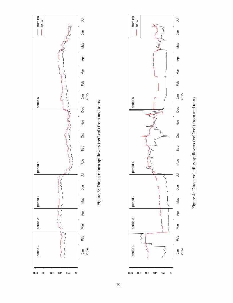
020406080100

Jan

Feb

Mar

Apr

May

Jun

Jul

Aug

Sep

Oct

Nov

Dec

Jan

Feb

Mar

Apr

May

Jun

Jul

2014

2015

perio

d 1

perio

d 2

perio

d 3

perio

d 4

perio

d 5

from

rts

to r

ts

Figu

re3:

Dir

ectr

etur

nsp

illov

ers

(ret

2vol

)fro

man

dto

rts

020406080100

Jan

Feb

Mar

Apr

May

Jun

Jul

Aug

Sep

Oct

Nov

Dec

Jan

Feb

Mar

Apr

May

Jun

Jul

2014

2015

perio

d 1

perio

d 2

perio

d 3

perio

d 4

perio

d 5

from

rts

to r

ts

Figu

re4:

Dir

ectv

olat

ility

spill

over

s(v

ol2v

ol)f

rom

and

tort

s

19

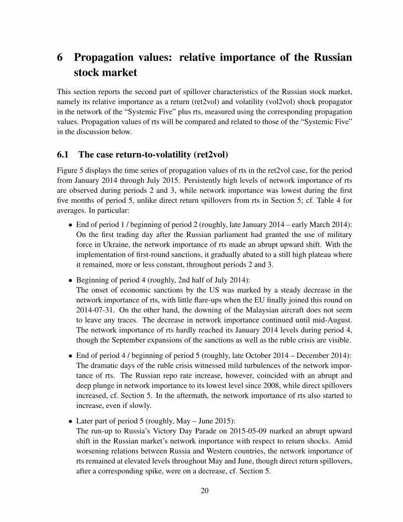
6 Propagation values: relative importance of the Russianstock market

This section reports the second part of spillover characteristics of the Russian stock market,namely its relative importance as a return (ret2vol) and volatility (vol2vol) shock propagatorin the network of the “Systemic Five” plus rts, measured using the corresponding propagationvalues. Propagation values of rts will be compared and related to those of the “Systemic Five”in the discussion below.

6.1 The case return-to-volatility (ret2vol)Figure 5 displays the time series of propagation values of rts in the ret2vol case, for the periodfrom January 2014 through July 2015. Persistently high levels of network importance of rtsare observed during periods 2 and 3, while network importance was lowest during the firstfive months of period 5, unlike direct return spillovers from rts in Section 5; cf. Table 4 foraverages. In particular:

• End of period 1 / beginning of period 2 (roughly, late January 2014 – early March 2014):On the first trading day after the Russian parliament had granted the use of militaryforce in Ukraine, the network importance of rts made an abrupt upward shift. With theimplementation of first-round sanctions, it gradually abated to a still high plateau whereit remained, more or less constant, throughout periods 2 and 3.

• Beginning of period 4 (roughly, 2nd half of July 2014):The onset of economic sanctions by the US was marked by a steady decrease in thenetwork importance of rts, with little flare-ups when the EU finally joined this round on2014-07-31. On the other hand, the downing of the Malaysian aircraft does not seemto leave any traces. The decrease in network importance continued until mid-August.The network importance of rts hardly reached its January 2014 levels during period 4,though the September expansions of the sanctions as well as the ruble crisis are visible.

• End of period 4 / beginning of period 5 (roughly, late October 2014 – December 2014):The dramatic days of the ruble crisis witnessed mild turbulences of the network impor-tance of rts. The Russian repo rate increase, however, coincided with an abrupt anddeep plunge in network importance to its lowest level since 2008, while direct spilloversincreased, cf. Section 5. In the aftermath, the network importance of rts also started toincrease, even if slowly.

• Later part of period 5 (roughly, May – June 2015):The run-up to Russia’s Victory Day Parade on 2015-05-09 marked an abrupt upwardshift in the Russian market’s network importance with respect to return shocks. Amidworsening relations between Russia and Western countries, the network importance ofrts remained at elevated levels throughout May and June, though direct return spillovers,after a corresponding spike, were on a decrease, cf. Section 5.

20

6.2 The case volatility-to-volatility (vol2vol)Figure 6 displays the time series of propagation values of rts in the vol2vol case, for the periodfrom January 2014 through July 2015. The overall pattern is similar to that of direct volatilityspillovers from rts in Section 5 (cf. Figure 4), with several notable differences. In detail:

• End of period 1 / beginning of period 2 (roughly, late January 2014 – early March 2014):The pattern of network importance of rts with respect to volatility shocks is similar tothat of direct volatility spillovers: a timely coincidence of boosts to a higher plateau andthe Russian rise of economic pressure on Ukraine in late January as well as the start ofthe Olympic Games in early February; and the Russian parliament’s authorization to useforce in Ukraine and the anticipation of sanctions sent network importance to a rollercoaster, too. As a result, however, propagation values did not fall below their January2014 levels, as did direct spillovers.

• Beginning of period 4 (roughly, 2nd half of July 2014):The network importance of rts rose again, unlike direct spillovers, on the occasions ofthe EU threat to impose sanctions in the immediate aftermath of the downing of theMalaysian aircraft and the sanction’s implementation on 2014-07-31. Also, networkimportance entered a turbulent phase.

• End of period 4 / beginning of period 5 (roughly, late October 2014 – December 2014):A strong upward shift in network importance of rts with respect to volatility shocks,much more pronounced than for volatility spillovers, coincided with Russia’s acknowl-edgment on 2014-12-02 that it was heading into a recession. News from China refueledconcerns and boosted the Russian market’s network importance on 2014-12-09. On2014-12-16, the day of the Russian repo rate increase, the network importance of rtssoared dramatically, to plunge to levels last witnessed during periods 2 and 3.

• Later part of period 5 (roughly, May – June 2015):The network importance of rts with respect to volatility shocks soared again on 2015-05-07, in the run-up to Russia’s Victory Day Parade, to build up even more and peakafter the EU’s “Eastern Partnership” summit on 2015-05-22, when Russia passed its billagainst “undesirable NGOs”. Network importance was diminishing again during June2015.

6.3 DiscussionIt turns out empirically that direct spillovers are not the same as propagation values, or relativenetwork importance, for example: ret2vol propagation values fell heavily when the CentralBank of Russia increased the repo rate (2014-12-16), while direct return spillovers rose. Otheroccasions saw direct spillovers from rts as well as its propagation values increasing, for exam-ple: the run-up to Victory Day Parade. This indicates a difference in how the network “digests”

21

return shocks in rts: below- (above-) average network repercussions when the repo rate wasincreased (in the run-up to Victory Day Parade, respectively). This aspect will be investigatedmore systematically in Section 7 below.

Although the behavior of ret2vol propagation values depends on the period, the series hasmuch less variability about its average than vol2vol propagation values; it hardly reaches be-yond 20% and never moves below 5%. The former series has relatively smaller level shifts,which, however, can be linked to important events, namely the Russian president’s parliamen-tary grant to use force in the Ukraine, the increase in repo rate, and the run-up to the RussianVictory Day Parade. The reaction of vol2vol propagation values to these stimuli has beenmuch more hefty; the series displays the biggest fluctuations during the third round of sanc-tions until the repo rate was increased. As in the case of direct spillovers, there is very littledifference between the first and second rounds of sanctions. The highest propagation valueswere the vol2vol propagation values during the onset of the Russian aggression (beyond 80%)and on the very day of the increase in repo rate (more than 60%): This is when a shock tothe volatility of the Russian stock market index rts had the relatively strongest impact on thenetwork.

Figures 7 and 8 show stacked plots of all the propagation value series concerning the net-work of the “Systemic Five” plus rts. By definition, propagation values sum up to 1 each day.These figures allow an assessment of the impact of other large-scale events and thus contributeto the interpretation of the propagation values of rts.

Concerning return shocks, Figure 7 reveals that the propagation values of the three Westernmarkets in the network (represented by dji, ftse, and sx5e) were almost at the same level andmore or less uniform across time, with a notable upward bulge at the expense of the Japaneseand Chinese markets in February 2014, coinciding with the Ukrainian revolution. This bulgewas followed by a plunge in early March 2014, mirroring the Russian market’s sudden boostin importance. — The Japanese stock market’s importance as propagator of return shocks,probably boosted in early 2014 by the introduction of the New Japan Stock Index,55 almostvanished in early March 2014, to appear again only a year later in March 2015 when a newcorporate governance code was to take effect.56 — News about weak economic indicators inlate 201457 may have shifted attention to China for some time, which is also clearly visible inFigure 7. Apart from these “Asian effects”, however, the pattern of propagation values of theRussian market can be linked to Ukraine- and Russia-related events.

Volatility shock propagation, on the other hand, paints a picture of sharp discontinuitiesat certain dates, affecting each member in the network; see Figure 8. The spikes relating tothe outright Russian threat of military intervention in Ukraine in early March 2014 and the

55“JPX-Nikkei Index 400”, start of calculation 2014-01-06; see Japan Exchange Group athttp://www.jpx.co.jp/english/markets/indices/jpx-nikkei400/index.html. Retrieved 2015-09-17.

56“Japans reforms push companies to unlock cash”, Financial Times, 2015-03-30; available onlineat http://www.ft.com/intl/cms/s/0/a5699738-ce58-11e4-86fc-00144feab7de.html#axzz3m1slR6H7. Retrieved2015-09-17.

57“China industrial activity shrinks in December, calls grow for more stimulus”, Reuters, 2014-12-16; avail-able online at http://www.reuters.com/article/2014/12/16/us-china-economy-pmi-idUSKBN0JU06520141216.Retrieved 2015-09-17.

22

repo rate increase in mid-December 2014 pinpoint the highly prominent role of the Russianmarket as volatility shock propagator in the network, in both cases marking the end of a phaseof elevated importance. In the latter case, however, the Russian market’s prominence hadmeanwhile been scaled down and even temporarily interrupted by global growth concerns anda plunge in stock prices in the US in mid-October 201458 and in China in early December201459, while the European markets’ role was waning. Figure 8 also unveils that the re-boostof the Russian market’s importance in early May 2015 was again Russia-related; news aboutfinancial reforms in China scaled it down only later in that month.60

period remarks ret2vol vol2vol0 before 2014 0.146 0.1431 2014, before sanctions 0.143 0.1482 first round of sanctions 0.180 0.0553 second round of sanctions 0.177 0.0644 third round of sanctions 0.135 0.1465 after increase in repo rate 0.123 0.085

Table 4: Average propagation values, rts

58“This is not another financial crisis”, CNN Money, 2014-10-15; available online athttp://money.cnn.com/2014/10/15/investing/stocks-plunge-not-like-2008/. Retrieved 2015-09-18.

59“Shanghai stocks suffer sharpest fall in five years”, Financial Times, 2014-12-09; available onlineat http://www.ft.com/intl/cms/s/0/95372ce6-7f79-11e4-b4f5-00144feabdc0.html#axzz3m1slR6H7. Retrieved2015-09-18.

60“China to allow individuals buy overseas financial assets”, Financial Times, 2015-05-29; available onlineat http://www.ft.com/intl/cms/s/0/5da9f1c4-05b5-11e5-bb7d-00144feabdc0.html#axzz3m1slR6H7. Retrieved2015-09-18.

23

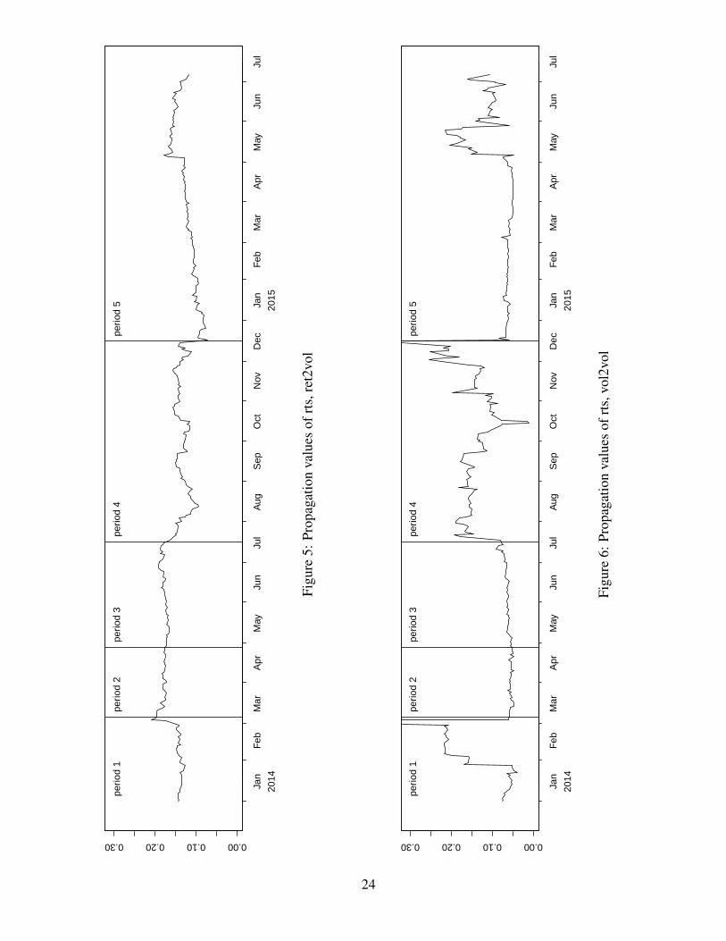
0.000.100.200.30

Jan

Feb

Mar

Apr

May

Jun

Jul

Aug

Sep

Oct

Nov

Dec

Jan

Feb

Mar

Apr

May

Jun

Jul

2014

2015

perio

d 1

perio

d 2

perio

d 3

perio

d 4

perio

d 5

Figu

re5:

Prop

agat

ion

valu

esof

rts,

ret2

vol

0.000.100.200.30

Jan

Feb

Mar

Apr

May

Jun

Jul

Aug

Sep

Oct

Nov

Dec

Jan

Feb

Mar

Apr

May

Jun

Jul

2014

2015

perio

d 1

perio

d 2

perio

d 3

perio

d 4

perio

d 5

Figu

re6:

Prop

agat

ion

valu

esof

rts,

vol2

vol

24

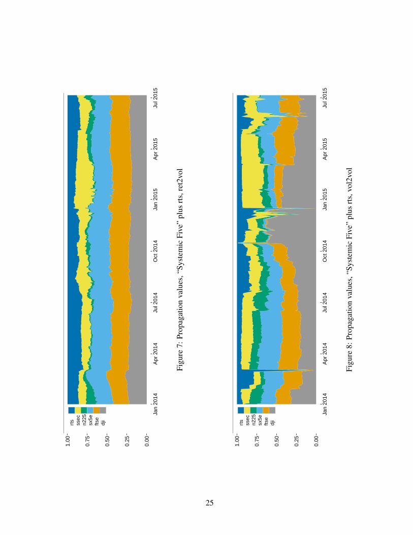
0.00

0.25

0.50

0.75

1.00

Jan

2014

Apr

201

4Ju

l 201

4O

ct 2

014

Jan

2015

Apr

201

5Ju

l 201

5

rts

ssec

n225

sx5e

ftse

dji

Figu

re7:

Prop

agat

ion

valu

es,“

Syst

emic

Five

”pl

usrt

s,re

t2vo

l

0.00

0.25

0.50

0.75

1.00

Jan

2014

Apr

201

4Ju

l 201

4O

ct 2

014

Jan

2015

Apr

201

5Ju

l 201

5

rts

ssec

n225

sx5e

ftse

dji

Figu

re8:

Prop

agat

ion

valu

es,“

Syst

emic

Five

”pl

usrt

s,vo

l2vo

l

25

7 Network repercussions of shocks in the Russian marketThis section reports the third part of spillover characteristics of the Russian stock market,namely network repercussions of return and volatility shocks in the Russian market.

Direct spillovers from the Russian market as well as the market’s propagation values havea distinct period-specific behavior, and the two series look very similar at first sight, but thereare notable differences between them. As was pointed out in Section 4, a direct comparisonof both series is not meaningful, while regression residuals are able to unveil whether directspillovers or network importance prevail at a given time. A residual close to zero indicatesthat direct spillovers and network importance are on a par, while positive (negative) residualsindicate that network importance (direct spillovers) outweighs direct spillovers (network im-portance, respectively). The two residual series (εt), one for each spillover perspective, areplotted in Figures 9 and 10 from 2014 onwards. The series have been standardized over theentire regression period, 1998 through 2015, in order to facilitate the comparison of repercus-sions from 2014 onwards with long-term repercussions. These series will be analyzed in thefollowing.

7.1 The case return-to-volatility (ret2vol)A plot of network repercussions of return shocks is shown in Figure 9. Again, periodic-specificbehavior is visible: regression residuals are close to zero in period 1; network repercussionswere prevailing throughout periods 2, 3 and 4, and direct spillovers dominated during the firstfive months of period 5. In particular:

• End of period 1 / beginning of period 2 (roughly, late January 2014 – early March 2014):When the Russian president openly declared his intention of military intervention inUkraine the first Saturday in March 2014, the anticipation and onset of sanctions the fol-lowing Thursday had a strong impact on the network in terms of heavy network reper-cussions of return shocks in the Russian market. This can be inferred from soaringregression residuals at that time. In the aftermath of the implementation of first-roundsanctions, network repercussions of return shocks in the Russian market were levelinglower, but were still elevated when compared to those earlier that year. Another peakoccurred on 2014-03-17, when sanctions were joined and extended by the EU. Networkrepercussions tended to grow during the following months.

• Beginning of period 4 (roughly, 2nd half of July 2014):The beginning of the third round of sanctions, first implemented by the US only, hasdiscontinued the preceding upward trend and entailed diminishing, but rather unstableamounts of network repercussions of return shocks in the Russian market. There was,however, a notable temporal peak in timely coincidence with the EU’s implementationof economic sanctions on 2014-07-31 (and yet another peak when they were extendedon 2014-09-12).

26

• End of period 4 / beginning of period 5 (roughly, late October 2014 – December 2014):Towards the end of period 4, return shocks in the Russian market started to leave strongeffects on the network again, peaking the day after Ukraine’s parliamentary election on2014-10-26, and refueled by concerns over Russia’s Ukraine politics. The ruble cri-sis and Russia’s bleak economic outlook in early December sent network repercussionslower, though first intervening efforts by the Central Bank of Russia (a lending-rateincrease) may have had a singular boosting effect. A huge temporary drop, taking re-gression residuals to a level far below zero, can be assigned to the day of the Russianrepo rate increase, leaving direct spillovers prevailing for several months.

• Later part of period 5 (roughly, May – June 2015):In the run-up to the Russian Victory Day Parade on 2015-05-09, another heavy boost ofnetwork repercussions of return shocks in the Russian market occurred, further buildingup during the subsequent two months and culminating on two occasions: one day in lateMay amid aggravated concerns of the Cold War resurging, when Russia was reportedto mass heavy firepower on its border with Ukraine, and another day in mid-June, on2015-06-19, when the annual St. Petersburg International Economic Forum just hadended, resulting in, among others, Russia’s declared willingness to intensify relationswith Greece.

7.2 The case volatility-to-volatility (vol2vol)The plot in Figure 10 of residuals in the case of a volatility shock in the Russian market reveals:The series of regression residuals is, with a few notable exceptions, close to zero, which showsthat (i) there is little difference between the long-term average (1998 through 2015) and theperiod beginning with 2014, (ii) propagation values with respect to volatility spillovers followthe direct spillovers closely. Particular exceptions are:

• End of period 1 / beginning of period 2 (roughly, late January 2014 – early March 2014):The Russian president’s openly declared intention of military intervention in Ukraine,just before the sanctions were implemented, is in timely coincidence with rising amountsof network repercussions of volatility shocks in the Russian market.

• Beginning of period 4 (roughly, 2nd half of July 2014):Network repercussions of volatility shocks in the Russian market made an abrupt up-ward shift on 2014-07-21, peaking the following day, when the EU agreed to imposenew sanctions on Russia, in particular threatening with economic sanctions if Russiawould not use its influence to restrain pro-Russian separatists believed to have downedthe Malaysia Airlines flight over Ukraine on 2014-07-17. Network repercussions grad-ually diminished in the aftermath, with moderate fresh peaks on 2014-07-31 (and on2014-09-15), that is, on the day (or the first trading day) after economic sanctions wereimplemented.

27

• End of period 4 / beginning of period 5 (roughly, late October 2014 – December 2014):December 2014 was a month of soaring network repercussions concerning volatilityshocks from rts, with a first spike on 2014-12-02, when Russia acknowledged that it washeading into a recession, and then on 2014-12-09, hitting its maximum, when concernsover Chinese economy and the World Bank’s revision of its growth projections for Rus-sia cumulated. The strong network repercussions on the day before the repo rate increasedied down abruptly on 2014-12-17, taking residuals temporarily far below zero.

• Later part of period 5 (roughly, May – June 2015):Another month of soaring network repercussions was May 2015, with a first abrupt riseon 2015-05-07 in the run-up to the Russian Victory Day Parade, and culminating, amidaggravated concerns of the Cold War resurging, on 2015-05-25, the first trading dayafter Russia’s passage of a bill against “undesirable NGOs”. Smaller repercussions wereprevailing during June.

28

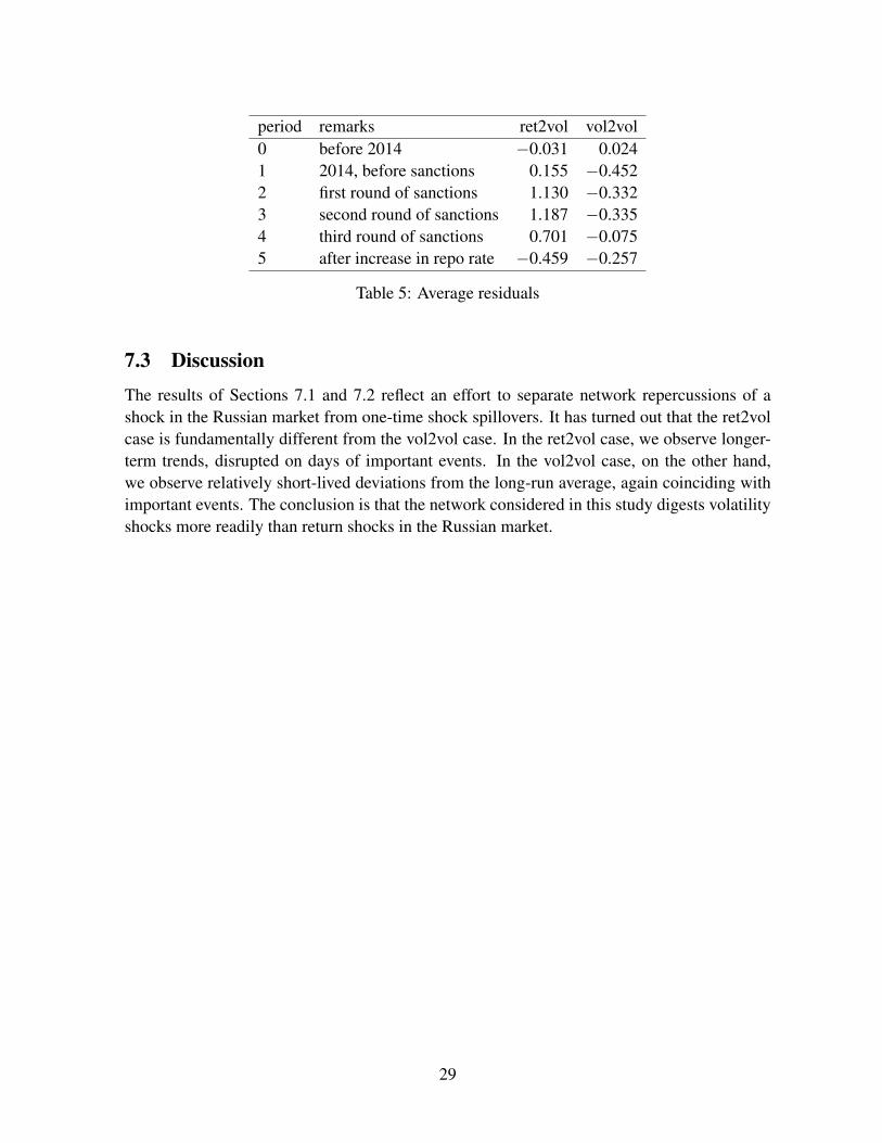
period remarks ret2vol vol2vol0 before 2014 −0.031 0.0241 2014, before sanctions 0.155 −0.4522 first round of sanctions 1.130 −0.3323 second round of sanctions 1.187 −0.3354 third round of sanctions 0.701 −0.0755 after increase in repo rate −0.459 −0.257

Table 5: Average residuals

7.3 DiscussionThe results of Sections 7.1 and 7.2 reflect an effort to separate network repercussions of ashock in the Russian market from one-time shock spillovers. It has turned out that the ret2volcase is fundamentally different from the vol2vol case. In the ret2vol case, we observe longer-term trends, disrupted on days of important events. In the vol2vol case, on the other hand,we observe relatively short-lived deviations from the long-run average, again coinciding withimportant events. The conclusion is that the network considered in this study digests volatilityshocks more readily than return shocks in the Russian market.

29

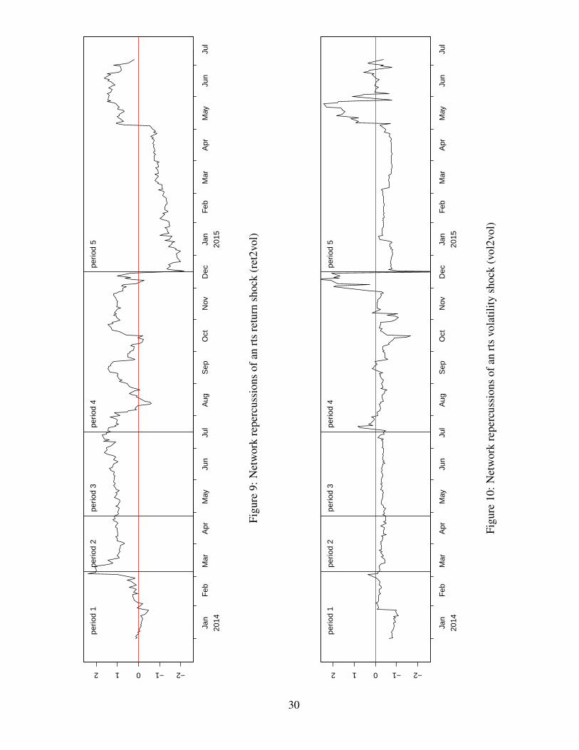
−2−1012

Jan

Feb

Mar

Apr

May

Jun

Jul

Aug

Sep

Oct

Nov

Dec

Jan

Feb

Mar

Apr

May

Jun

Jul

2014

2015

perio

d 1

perio

d 2

perio

d 3

perio

d 4

perio

d 5

Figu

re9:

Net

wor

kre

perc

ussi

ons

ofan

rts

retu

rnsh

ock

(ret

2vol

)

−2−1012

Jan

Feb

Mar

Apr

May

Jun

Jul

Aug

Sep

Oct

Nov

Dec

Jan

Feb

Mar

Apr

May

Jun

Jul

2014

2015

perio

d 1

perio

d 2

perio

d 3

perio

d 4

perio

d 5

Figu

re10

:Net

wor

kre

perc

ussi

ons

ofan

rts

vola

tility

shoc

k(v

ol2v

ol)

30

8 Summary and conclusionsWe studied the stock market network of the “Systemic Five” plus Russia, that is: the USA(represented by dji), the UK (ftse), the euro area (sx5e), Japan (n225), China (ssec), and Rus-sia (rts). In particular focusing on the period from January 2014 through July 2015, we areinterested in gauging shock spillover characteristics of the Russian market in the light of eventsand international sanctions in connection with the Ukrainian crisis, with a focus on detectingdifferences between different rounds of sanctions.

The methodology of this paper uses, and extends, methodology developed by Dieboldand Yilmaz (2009, 2014). It permits daily screening of network dynamics in terms of directreturn-to-volatility (and volatility-to-volatility) spillovers from and to rts as well as in terms ofrepercussions of return (and volatility) shocks coming from rts. The latter is measured by aconcept called the propagation value in the present paper; it measures the relative importanceof a shock in a market as seed for future uncertainty in returns (and volatilities) across thenetwork. Together with direct spillovers, this also allows an assessment of whether directspillovers, or network repercussions of shocks, are more important on a given day.

There is strong evidence that political and economic events, along with the internationalsanctions imposed so far in connection with the Ukrainian crisis, impacted shock spillovercharacteristics of the Russian stock market.

On the one hand, we found period-specific behavior of direct spillovers and propagationvalues with respect to rounds of sanctions, concerning both return and volatility shocks in rts.While rounds 1 and 2 of the sanctions hardly differ with respect to their patterns, these changetotally with the implementation of economic sanctions in round 3, and again after the CentralBank of Russia increased the weekly repo rate. When round 3 of sanctions commenced, directspillovers as well as propagation values from return shocks in rts slumped back to the lowlevels held before the sanctions began (or to even lower levels), while those from volatilityshocks entered a period of turbulence on elevated levels. This period ends abruptly with theday when the Central Bank of Russia increased the repo rate. In the aftermath, the impactof volatility shocks in rts on the network was reduced considerably, while return shocks werebecoming more important again, though only with respect to direct spillovers: the propagationvalue of return (and volatility) shocks in rts initially plunged to its lowest level.

On the other hand, there are five prominent events, among them the repo rate increase, thatcoincided with a sudden burst or downturn in network repercussions. Russia’s propagationvalues fell heavily when the Central Bank of Russia increased the repo rate, leaving networkrepercussions far below average. Two other events, of direct economic relevance, with strongimpact on volatility shocks and network repercussions were the threat of economic sanctionsby the EU after the downing of the Malaysian aircraft in July 2014, and Russia’s acknowledg-ment that it was heading into a recession in early December 2014. The remaining two events,of a more political character, lead to bursts of network repercussions which were particularlypronounced for return shocks: the Russian president’s parliamentary pledge and grant to useforce in Ukraine in early March 2014, and Russia’s activities around the Victory Day Parade inMay 2015; no other Victory Day since 1998 had such a big impact. This indicates a difference

31

in how the network “digests” news.In 2014, Russia’s GDP was down by 11.26% compared to 201361, and its trading volume

with the EU had decreased to c. EUR 300 bn62. An analysis of the costs of the trade restrictionsbetween the EU-27 plus Switzerland versus Russia was conducted in a recent study, see Chris-ten et al. (2015). According to them, EU-27 plus Switzerland economies are estimated to incurshort-run costs of EUR 34 bn in the value added; similarly, the long-run costs are estimated toamount to EUR 92 bn.

Economic sanctions did not isolate Russia, but they did change its role as a shock prop-agator in the network of stock markets: They reduced the Russian stock market’s relativeimportance as a propagator of return shocks. We have shown that this reduction came at thecost of increasing the importance of the Russian stock market as a propagator of volatilityshocks, thereby increasing the risk across the network. The deterioration of the Russian econ-omy, along with the ruble’s depreciation, could be responsible for this phenomenon; indeed,fears of a 1990s type contagion effects were pronounced louder than before. With this ob-servation in mind, it can be concluded that sanctions can be used as a policy tool to imposecosts on the sanctioned economy. Sanctions are able to magnify an economy’s problems. Butthis can probably only be achieved at the expense of introducing more volatility into the entirenetwork of stock markets and, in particular, making the network more vulnerable with respectto volatility shocks from the Russian stock market, to the effect that the sanctioning economiesare faced with a backlash of their own sanctions.

61Own calculations, based on data provided by the World Bank; see http://data.worldbank.org/data-catalog/GDP-ranking-table. Retrieved 2015-05-21.

62“European Union, Trade in goods with Russia”, released by the European Commission; available online athttp://trade.ec.europa.eu/doclib/docs/2006/september/tradoc 113440.pdf. Retrieved 2015-10-04

32

ReferencesAloui, R., Aissa, M.S.B., Nguyen, D.K. (2011). Global financial crisis, extreme interdepen-

dences, and contagion effects: The role of economic structure? Journal of Banking andFinance, 35, 130–141.

Bonacich, P., 1987. Power and centrality: a family of measures. American Journal of Sociology92, 1170–1182.

Christen, E., Fritz, O., Streicher G., 2015. Effects of the EU-Russia Economic Sanctions onValue Added and Employment in the European Union and Switzerland. Austrian Instituteof Economic Research, monograph, June 2015, 24 pages.

Diebold, F.X., Yilmaz, K., 2009. Measuring Financial Asset Return and Volatility Spillovers,with Application to Global Equity Markets. Economic Journal 119, 158–171.

Diebold, F.X., Yilmaz, K., 2014. On The Network Topology of Variance Decompositions:Measuring The Connectedness of Financial Firms. Journal of Econometrics 182 (1), 119–134.

German, M.B. and Klass, M.J. (1980): On the estimation of security price volatilities fromhistorical data, Journal of Business, 53 (1), 67–78.

International Monetary Fund (Ed.), 2011. 2011 Consolidated Spillover Report: ImplicationsFrom The Analysis of The Systemic-5. International Monetary Fund, Washington D.C.

International Monetary Fund (Ed.), 2012. 2012 Spillover Report – Background Papers. Inter-national Monetary Fund, Washington D.C.

Lutkepohl, H., 2005. New Introduction to Multiple Time Series Analysis. Springer, New York.

Pesaran, H.H., Shin, Y., 1998. Generalized Impulse Response Analysis in Linear MultivariateModels. Economics Letters 58, 17–29.

Pinto, B., Ulatov, S., 2010. Financial Globalization and the Russian Crisis of 1998. The WorldBank Policy Research Working Paper 5312.

R Core Team, 2015. R: A Language and Environment for Statistical Computing. R Foundationfor Statistical Computing, Vienna, Austria.

Schmidbauer, H., Rosch, A., Uluceviz, E., 2013a. Information Propagation between EquityMarkets: the Case of BRICT. In: EcoMod Network (ed.), Proceedings of the InternationalConference on Policy Modeling EcoMod 2013, Prague, Czech Republic, July 1-3, 2013.Online, http://ecomod.net/conferences/ecomod2013?tab=downloads.

33

Schmidbauer, H., Rosch, A., Uluceviz, E., 2013b. Market Connectedness: Spillovers, Infor-mation Flow, and Relative Market Entropy. Koc University – TUSIAD Economic ResearchForum, Working Paper 1320 (October 2013).Online, http://eaf.ku.edu.tr/sites/eaf.ku.edu.tr/files/erf wp 1320.pdf

Scott, H.S., 2014. Interconnectedness and Contagion — Financial Panics and the Crisis of2008. Working paper, available at SSRN: http://ssrn.com/abstract=2178475.

34