Essays in Behavioural Finance and Investment · Essays in Behavioural Finance and Investment A...

I

Essays in Behavioural Finance and Investment

A thesis submitted for the Degree of Doctor of Philosophy

By

Mohamed Ahmed Shaker Ahmed

Department of Economics and Finance

College of Business, Arts and Social Sciences

Brunel University London

London, United Kingdom

June 2017

II

Abstract

This thesis is an attempt to bridge some research gaps in the area of behavioural finance

and investment through adopting the three essays scheme of PhD dissertations.

There is a widespread belief that the traditional finance theory failed to provide a

sufficient and plausible explanation for (1) what motivates individual investors to trade, (2)

the pattern of their trading and the formation of their portfolios, (3) the determinants of cross

section of expected returns other than risk. Behavioural Finance, however, offers more

realistic assumptions based on two building blocks; behavioural biases of irrational investors

and the limits of arbitrage that prevent the arbitrageurs from correcting mispricing and

pushing prices back to fundamental values. This dissertation is structured as follows:

In the first essay, the disposition effect is defined as the propensity of investors to

realize gains too early while being loath to realize losses. Capital gains overhang is a measure

of unrealized capital gains and losses that is associated with the disposition effect and the

trading activities of behaviourally biased investors. We discover that firm characteristics can

play a role in explaining variations in the capital gains overhang that is consistent with the

activities of behaviourally biased and disposition investors. Specifically, we find that capital

gains overhang is increasing in firm attributes that attract behaviourally biased investors,

namely, earnings per share, leverage, growth and size. Capital gains overhang is also

declining in market liquidity, possibly because liquidity allows behaviourally biased investors

to excessively trade shares and beta and corporate earnings, probably because when high risk

and inefficient firms experience losses, disposition investors experience capital losses that

they are reluctant to realize.

In the second essay, quantile regressions are employed to analyse the relationship

between the unrealized capital gains overhang and expected returns. The ability of the

disposition effect to generate momentum is also considered for the extreme expected return

regions (0.05th

) and (0.95th

) quantiles. To do so, 450,617 observations belonging to 5176 US

firms are employed, covering a time span from January 1998 to June 2015. Following the

methodology of Grinblatt and Han (2005), the findings show significant differences across

various quantiles in terms of signs and magnitudes. These findings indicate a nonlinear

relationship between capital gains overhang and expected returns since the impact of capital

gains overhang as a proxy for disposition effect on expected returns vary across the expected

III

return distribution. More precisely, the coefficients of capital gains overhang are significantly

positive and decline as the expected returns quantiles increase from the lowest to the median

expected return quantiles. However, they become significantly negative and rise with the

increase in expected returns quantiles above median expected returns quantiles. The findings

also suggest that the disposition effect is not a good noisy proxy for momentum at the lowest

expected return quantile (0.05th

). However, interestingly it seems to generate contrarian in

returns at the highest expected returns quantile (0.95th

).

In the third essays, we try to discover systematic disagreements in momentum,

asymmetric volatility and the idiosyncratic risk-momentum return relationship between high-

tech stocks and low-tech stocks. We develop several hypotheses that suggest greater

momentum profits, fainter asymmetric volatility and weaker idiosyncratic risk-momentum

return relation in the high-tech stocks relative to the low-tech stocks. To this end, we divide

5795 stocks that are listed in the Russell 3000 index from January 1995 to December 2015

into two samples SIC code and analysed them using the Fama-French with GJR-GARCH-M

term. The results show that the high-tech stocks provide greater momentum profits especially

for portfolios that have holding and ranking periods of less than 12 months. In most cases

momentum returns in the high-tech stocks explain a symmetric response to good and bad

news while the momentum returns in the low-tech stocks show an asymmetric response.

Finally, the idiosyncratic risk-momentum return relation is insignificant for high-tech stocks

while it is significant and negative for low-tech stocks. That is, as idiosyncratic risk increases,

momentum decreases for low-tech stocks. These findings are robust to different momentum

strategies and to different breakpoints.

IV

Dedicated to my Family

V

Acknowledgement

Doing a PhD is a demanding journey: it is an unsteady road and you cannot see the

light at the end of the tunnel. Thanks should go to many people who supported me during this

journey.

First and foremost, I would like to deeply thank Professor Frank Skinner, my PhD

principal supervisor, for being very close and supportive. Professor Frank has indeed been an

excellent academic expert and magnificent supervisor. I have benefited enormously from his

openness, guidance and constructive feedback throughout my PhD journey. I would also like

to thank Dr. Qiwei Chen, my second supervisor, for attending almost all meetings and for

giving me her fruitful comments and constant feedbacks. Her valuable advice was of crucial

importance for the timely completion of this thesis. I am indebted to the vibrant environment

I experienced at Brunel University London. All the useful comments I received in seminars

and discussions have contributed greatly to my research efforts.

My deepest appreciation goes to Dr. Ahmed G. Radwan who helped me with

MATLAB and Dr Khairy Elgiziry who acted as an Egyptian supervisor before I transfer my

registration to Brunel University. I am also grateful to Dr. Ahmed Fahmy, Dr. Amr Kotb, Dr.

Khaled Hussainey and Dr. Wael Kortam who supported me during the process of applying

for and processing my governmental scholarship.

My friends from the doctoral programme, Ali Shaddady, Mohamed Husam Helmi, and

Ahmed Al-Saraireh, among others also gave crucial motivation on my PhD journey. I owe

my deepest gratitude to my family. In particular, thanks go to my father and mother for

making Du‟aa and for their endless emotional and financial care. Mahmoud Shaker and my

sisters deserve special thanks for their helpful attitude. I cannot forget to thank my kind-

hearted cousins Elbadry Mohamed and Hassan Ali for their unstoppable eagerness to

motivate and support.

Last, but not least, I would like to extend my grateful appreciation to the Egyptian

Ministry of Higher Education and all staff members of the Egyptian Cultural and Educational

Bureau in London for the financial support and PhD scholarship I was granted and feel

grateful to Dr Reem Bahgat, the Cultural Counsellor, for her support and encouragement.

Finally, I thank Yacine Belghitar (Cranfield University) and Nicola Spagnolo (Brunel

University London) for their useful comments in the course of my PhD defence in May 2017.

Mohamed Ahmed

June 2017

VI

Declaration

“I certify that this work has not been accepted in substance for any degree, and is not

concurrently being submitted for any degree or award, other than that of the PhD, being

studied at Brunel University London. I declare that all the material presented for examination

is entirely the result of my own investigations except where otherwise identified by

references and that I have not plagiarised another‟s work. In this regard, this thesis has been

evaluated for originality checking by the University library through Turnitin plagiarism

detection software prior to the formal submission. I also grant powers of discretion to the

University Librarian to allow this thesis to be copied in whole or in part without the necessity

to contact me for permission. This permission covers only single copies made for study

purpose subject to the normal conditions of acknowledgement.”

VII

Table of Contents Abstract ..................................................................................................................................... II

Acknowledgement .................................................................................................................... V

Declaration ............................................................................................................................... VI

Table of Contents ................................................................................................................... VII

List of Tables ........................................................................................................................... IX

Chapter One

Introduction

1.1- Motivation of the thesis .................................................................................................. 1

1.2- Towards a behavioural paradigm shift ............................................................................ 2

1.3- Overview of the thesis .................................................................................................... 6

Chapter Two

Data

2.1-Sample Selection ............................................................................................................ 13

2.2- Descriptive Statistics ..................................................................................................... 15

Tables of results ................................................................................................................... 16

Chapter Three

Determinants of Capital gains overhang

Abstract ................................................................................................................................ 19

3.1- Introduction ................................................................................................................... 20

3.2- Literature review ........................................................................................................... 23

3.3- Hypotheses Development ............................................................................................. 27

3.4- Description of the sample and methodology ................................................................ 30

3.5- Empirical analysis ......................................................................................................... 34

3.6- Conclusion .................................................................................................................... 36


Chapter Four

Revisiting disposition effect and momentum: A quantile regression perspective

Abstract ................................................................................................................................ 50

4.1- Introduction and Background ....................................................................................... 51

4.2- Hypotheses Development ............................................................................................. 54

4.3- Quantile regression technique ....................................................................................... 56

4.3.1- OLS and LAD ........................................................................................................ 56

VIII

4.3.2- Quantile regression model ...................................................................................... 56

4.4- Data, sample and methodology description .................................................................. 57


4.5.1– Descriptive statistics .............................................................................................. 59

4.5.2- The cross sectional determinants of unrealized capital gains overhang ................. 60

4.5.3- Expected returns, past returns and unrealized capital gains ................................... 62

4.6- Disposition effect and momentum ................................................................................ 63

4.7- Conclusion .................................................................................................................... 66


Chapter Five

Momentum, asymmetric volatility and idiosyncratic risk: A comparison of high-tech and low-

tech stocks

Abstract ................................................................................................................................ 83

5.1- Introduction ................................................................................................................... 84

5.2- Literature review ........................................................................................................... 87

5.2.1- Momentum ............................................................................................................. 88

5.2.2- Asymmetric volatility ............................................................................................. 88

5.2.3- Idiosyncratic risk -momentum return relation ........................................................ 90

5.3- Hypotheses development .............................................................................................. 92

5.4- Econometric framework................................................................................................ 96

5.4.1- The GARCH in mean („GARCH-M‟) model ......................................................... 96

5.4.2- The GJR –GARCH-M model ................................................................................. 96

5.5- Data and methodology .................................................................................................. 97


5.6.1- Summary statistics.................................................................................................. 98

5.6.2- Momentum ........................................................................................................... 100

5.6.3 Asymmetric volatility ............................................................................................ 101

5.6.4- Idiosyncratic risk -momentum return relation ...................................................... 103

5.6.5- The Performance of Fama-French model ............................................................. 105

5.7- Conclusion .................................................................................................................. 106

Tables of results ................................................................................................................. 108

Chapter Six

Concluding Remarks .............................................................................................................. 127

Bibliography .......................................................................................................................... 131

IX

List of Tables

Table 2.1. A description of the variables. ................................................................................ 16

Table 2.1. (Continued) ............................................................................................................. 17

Table 2.2. Summary statistics .................................................................................................. 18

Table 3.1. A description of the variables ................................................................................. 38

Table 3.2. Descriptive statistics ............................................................................................... 39

Table 3.4. Correlation Matrix .................................................................................................. 41

Table 3.5. Panel regression output ........................................................................................... 42

Table 3.6. Robustness analysis based on cross section regression (year by year) ................... 43

Table 3.7. Robustness analysis based on growth subsamples ................................................. 44

Table 3.8. Robustness analysis based on beta subsamples ...................................................... 45

Table 3.9. Robustness analysis based on size subsamples....................................................... 46

Table 3.10. Robustness analysis based on turnover subsamples ............................................. 47

Table 3.11. Robustness analysis based on before and after financial crisis subsamples ......... 48

Table 3.12. Robustness analysis based on capital gains/losses subsamples ............................ 49

Table 4.1. Description of the independent variables................................................................ 67

Table 4.2. Summary statistics .................................................................................................. 68

Table 4.3. Correlation matrices and Heteroscedasticity .......................................................... 69

Table 4.4. Determinants of capital gains overhang: Fama-MacBeth and Quantile regression 70

Table 4.5. Determinants of Capital gains overhang: Robustness analysis based on institutional

ownership subsamples ............................................................................................................. 71

Table 4.6. Determinants of Capital gains overhang: Robustness analysis based on leverage

subsamples ............................................................................................................................... 72

Table 4.7. Determinants of Capital gains overhang: Robustness analysis based on size

subsamples ............................................................................................................................... 73

Table 4.8. Expected returns, past returns and capital gains overhang: Comparison between

Fama-MacBeth two step procedure and quantile regression ................................................... 74

Table 4.9. Expected returns, past returns and capital gains overhang: February to November

subsample ................................................................................................................................. 75

Table 4.10. Expected returns, past returns and capital gains overhang: January and December

subsamples ............................................................................................................................... 76

Table 4.11. Expected returns, past returns and unrealized capital gains: Robustness analysis

based on institutional ownership subsamples .......................................................................... 77

X


based on leverage subsamples ................................................................................................. 78


based on size subsamples ......................................................................................................... 79

Table 4.14. Capital gains coefficients across three models ..................................................... 80

Table 4.15. Capital gains coefficients across different quantiles............................................ 81

Table 4.16. Tests of the equality-of-slope estimates across quantiles between expected

returns and capital gains overhang ........................................................................................... 82

Table 5.1. Description of the independent variables.............................................................. 108

Table 5.2. Summarizes the proportion of each industry in the high-tech stocks versus low-

tech stocks .............................................................................................................................. 109

Table 5.2. (continued) ............................................................................................................ 110

Table 5.3. Unit root test (Augmented Dickey-Fuller) Breakpoint 10% ................................ 111

Table 5.4. Unit root test (Augmented Dickey-Fuller) Breakpoint 30% ................................ 112

Table 5.5. ARCH effect „10% Breakpoint‟ ........................................................................... 113

Table 5.6. ARCH effect „30% Breakpoint‟ ........................................................................... 114

Table 5.7. portfolios characteristics based on 6-6 momentum strategy using 10% breakpoint

................................................................................................................................................ 115

Table 5.7. (Continued) ........................................................................................................... 116

Panel B: t-statistics for each portfolio and each factor .......................................................... 116

Table 5.8. Summary statistics of momentum portfolios based on 10% breakpoint .............. 117

Table 5.9. Summary statistics of momentum portfolios: Robustness analysis based on 30%

breakpoint .............................................................................................................................. 118

Table 5.10. Fama-French with a GJR-GARCH-M based on 10% breakpoint ...................... 119

Table 5.10. (Continued) ......................................................................................................... 120

Table 5.11. Fama-French with a GJR-GARCH-M: Robustness analysis based on 30%

breakpoint .............................................................................................................................. 121

Table 5.11. (Continued) ........................................................................................................ 122

Table 5.12. Fama-French with a GARCH (1,1)-M based on 10% breakpoint ...................... 123

Table 5.12. (Continued) ......................................................................................................... 124

Table 5.13. Fama-French with a GARCH (1,1)-M: Robustness analysis based on 30%

breakpoint .............................................................................................................................. 125

Table 5.13. (Continued) ......................................................................................................... 126

1

Chapter One

Introduction

The objective of this chapter is to present an overview of this thesis. In the first section,

the motivation of the thesis is presented. In the second section, the theoretical development

towards the behavioural paradigm shift is outlined. In the third section, we introduce an

overview of the thesis including the research motivation, the objectives of each empirical

paper, key contributions and main findings.

1.1- Motivation of the thesis

Traditional finance assumes that we are rational, while behavioural finance

assumes we are normal.

____Meir Statman1

The first and foremost motivation of this thesis is the unrealistic assumptions of the

standard finance based on CAPM/EMH framework. The standard finance studies financial

phenomena assuming all investors are rational, well-informed, process all available

information properly, process it and take rational decisions. Empirical evidence in the

literature denied these assumptions and documented that investors oftentimes behave

differently.

Behavioural finance, however, is a research discipline that uses psychological theories

for explaining and understanding investment decision-making. It studies finance from wider

perspective that intersects finance and economics with psychology and sociology. In contrast

to standard finance, the necessity of behavioural finance comes from a considerable amount

of literature in psychology revealed that people commit systematic cognitive errors in

decision making process based on bounded rationality and cognitive limitations. These errors

stem from investors‟ preferences or improper beliefs such as overconfidence, regret

avoidance, fear of loss, disposition effect, framing, mental accounting, naïve diversification,

anchoring, availability bias, representativeness bias and conservatism bias, and cause

impermanent excess supply or excess demand leading to temporary mispricing. Another

1 See Gregory Curtis (2004) P.16

2

rationale for the necessity of behavioural finance is financial anomalies. Theses anomalies

can be defined as systematic empirical patterns that are explained by traditional CAPM/EMH

framework such as momentum, size effect, value effect and turn-of-the-year. While the

CAPM was genuine idea to capture the risk-return relationship, it experienced many

empirical failures in explaining such anomalies.

Additionally, under the framework of standard finance it is often said arbitrageurs sell

overpriced stock short and buy underpriced stocks long to correct any mispricing caused by

irrational investors who prone to cognitive errors. This claim is unrealistic due to risk

embodied in the long and short position or constraints on short selling or implementation

cost. Moreover, arbitrageurs sometimes prefer not to trade or enter the market when the

mispricing is too large.

1.2- Towards a behavioural paradigm shift

The clue of efficient market hypothesis devised by Eugene Fama first appeared in

Journal of Business (1965). According to this hypothesis, Stock prices reflect all available

information on capital assets (Frankfurter & McGoun, 2002). Fama (1970) then developed

three different forms of informational efficiency, namely, weak form, semi-strong and strong

market efficiency.

Weak Form Market Efficiency- The current stock price fully reflects all information

embodied in historical prices and volume.

Semi-Strong Market Efficiency- the current stock price reflects historical price and volume

data as well as all publically available information including news, analysts‟ reports and

company reports.

Strong Market efficiency- The current stock price reflects not only historical price and

volume data, but also all public and private information.

Sharpe (1964) and Lintner (1965) develop the capital asset pricing model (CAPM)

which is an intuitive model to measure the investment risk and to capture the relation

between risk and expected returns. The CAPM depends on three assumptions: first, the

capital market is perfect which means there are no transaction cost or taxes and information is

3

available and can be obtained without costs. As a result, investors can lend and borrow at the

risk-free rate. Second, the homogenous expectation assumption; this assumption is that all

investors have the same expectations, and they are all rational and they are risk-averse. Third,

the CAPM assumes all investors have only one holding period and they use expected return

and standard deviation of return in evaluating their portfolios (Perold, 2004). However, the

empirical tests indicate that unsatisfying performance of the CAPM is attributable to the very

simplified and unrealistic assumptions (Fama & French, 2004). The efficient market

hypothesis (EMH) and the capital asset pricing model (CAPM) framework are the hub of

standard finance theory (Statman, 1999) and the word „anomaly‟ is always used to refers to

the stream of research that focuses on the empirical invalidity of EMH/CAPM framework.

Schwert (2003) provides a comprehensive summary of all anomalies in finance

literature on the following lines:

Size effect- the term size effect is used to point out the negative relation between size and

average returns. Banz (1981) proved that small firms provide 0.40% higher average monthly

returns than the other stocks did, using data on NYSE from 1936 to 19752. Reinganum (1981)

empirically supports the same anomaly through proving the small firms give higher average

returns than large firms do.

The value effect- the value effect is used to point out that the firms with high ratios of

Earnings to price (E/P) and book-to-market provide higher average returns than firms with

low ratios of Earnings to price (E/P) and book-to-market ratio do. Basu (1977) in his seminal

paper was the first to document the value effect. Basu (1977) found that stocks with higher

value-related variables such as earnings per share (P/E) can make positive abnormal returns.

He also confirmed that the CAPM could not provide an explanation for this behaviour.

Momentum effect- Jegadees & Titman (1993) form wide range of momentum strategies

using market data from 1965 to 1989. They reveal that momentum strategies which entail

buying past winners (stocks that have high returns over the previous three months to one

year) and selling past losers (stocks that have low returns over the previous three months to

one year) can generate monthly average returns of 1% for the next year.

2 See Van Dijk (2011) P.3264

4

The turn-of-the-year effect / ‘January Effect’- this anomaly has two interpretations: the

first hypothesis is the tax-loss-selling-pressure hypothesis. According to this hypothesis,

individual investors tend to realize capital losses by selling stocks that have gone down in

prices during the year. These capital losses help them reduce their year-end tax liability and

create selling pressure through an increase in the number of transactions, leading to a drop in

year-end stock prices (Berges, McConnell, & Schlarbaum, 1984). The second hypothesis is

the window dressing hypothesis. According to this hypothesis, institutional investors tend to

rebalance their portfolio holdings before the end of the year through selling losers and buying

winners, hoping to enhance the perceived performance (Haug & Hirschey, 2006).

The weekend effect- French (1980) is the first to use the term „weekend effect‟. He

employed data on S&P 500 composite index from 1953 through 1977, and found negative

average returns on Mondays and positive otherwise.

The empirical success of previous anomalies and the challenging role they play in the

traditional framework EMH/CAPM show the need for a change from traditional framework

EMH/CAPM to behavioural theory. The behavioural theory of finance has two pillars:

Limits to arbitrage- Shleifer & Vishny (1997) criticize the description of arbitrage as a no

capital and no risk process which entails buying and selling similar financial security in two

different markets to make profits through benefiting from different prices. Traditional finance

assumes that arbitrage mechanism maintains market efficiency by assuming investors

mistakes would impact on the market prices and pushing prices away from the fundamental

value, while arbitrageurs -„rational investors‟- are always going to benefit from any

mispricing to make profits and correct any devation from the fundemental value. However,

behavioural finance defenders believe that market prices are not fair.

In theory institutional investors play the role of rational investors because they have the

required knowledge, analysts and wealth but they also have benefits to urge the way of

trading that causes mispricing and motivates inefficiency (Baker & Nofsinger 2010). Barberis

& Thaler (2003) mention that the limits to arbitrage that may prevent arbitrage and keep the

market inefficient include: (1) fundamental risk because the short and long positions are

prone to mismatch; (2) noise trader risk because the mispicing could be too large to be

corrected and may lead to bankrupting the arbitrageurs; (3) Implementation cost. Thus, the

limits to arbitrage may hinder the arbitrageurs from correcting any mispricing.

5

Behavioural biases- Ritter (2003) lists the key behavioural biases in the literature of

behavioural finance as follows:

1- Heuristics or rules of thumb: the employment of rules of thumb facilitates the

decision making process but can also cause cognitive biases. Benartzi and Thaler (2001)

discover that several investors follow the 1/N rule. For instance, if they encounter three

alternatives that are available for investing their money, they allocate one-third of their

money to each fund3.

2- Overconfidence: overconfidence means that people sometimes overestimate their skills

and capabilities. There are several forms of overconfidence such as insufficient

diversification that may lead investors to over-invest in one asset. For instance, the finance

literature documents that men are usually have higher levels of confidence than women

but that women tend to outperform men.

3- Mental Accounting: mental accounting means that people tend to split decisions that

should not be split. This may also lead to cognitive biases, for example, if several people

allocate separate budgets for food and entertainment. They eat simple fish at home

because shrimp is more expensive than fish but they prefer to eat shrimp at restaurant

although the cost is higher than that of simple fish. If they combined eating at home and in

restaurants they could save money through choosing to have shrimp at home and simple

fish in restaurants.

4- Framing : framing concerns how an idea or term is exhibited to people. In other words,

it deals with ways of expression. For instance, cognitive pychologists found that doctors

give one set of prescriptions and treatments if a diagnosis is presented in the form of

survival probabilities and another set if it is presented in the form of mortality probabilities

in spite of the fact that the survival probabilities and mortality probabilities together

totalled 100%.

5- Representativeness /‘Law of small numbers’: representativeness means that people

have a propensity to overweigh contemporary events and underweigh ancient events. For

instance, if the equities generate a high return for many years in succession, some

investors start to believe that a high average return is customary.

3 See Ritter (2003) P. 431.

6

6- Conservatism: representativess and conservatisim battle against each other. While

representativeness leads to underweighing rates, people sometimes romanticize the base

rates. In other words, when a change occurs, people tend to stick to the initial values and

react slowly to the change. Therefore, the consevatism bias can be considered one source

of underreaction.

7- Dissposition effect: the disposition effect is the tendency of investors to realize gains

too early and hold losers too long. For instance, if somebody purchases a stock at $10,

which then goes down to $6 before going up to $8, most people are not willing to sell until

the stock price exceeds $10. Through the disposition effect, investors try to realize plenty

of small gains, and a few minimal losses. In other words, their decision conforms with

taxes maximization behaviour. The disposition effect comes out in aggregate trading

volume since stocks tend to have a higher trading volume during bull markets and a lower

trading volume during bear markets.

1.3- Overview of the thesis

The main focus of this thesis is to shed more light on the field of behavioural finance as

one of the most important topics in finance theory. In doing so, the researcher submits three

empirical papers and adds a chapter for data. The overall structure is as follows:

In Chapter 2, we provide a brief description of the Russell 3000 index together with its

key characteristics; it is used throughout the thesis. The survivorship bias and some potential

ruinous effects of survivorship bias are discussed and reviewed in chapter 2, since we

updated our list of stocks each month to free our dataset from survivorship bias. Finally, this

chapter details the definitions of all the variables used throughout the thesis and gives some

descriptive statistics for each variable.

The main motivation of chapter 3 is, there was a belief in the literature that irrational

investors trade randomly and there is no systematic pattern beyond their trading. We

motivated by whether the irrational investor trade systematically or not.

Chapter 3 is dedicated to testing whether or not irrational investors prefer to buy and

keep stocks of good companies. As a result, a number of characteristics of good companies

are chosen such as their earnings per share („EPS‟) as proxy for profitability, leverage as

proxy for debt burden of a company, cash flow to price as a proxy for corporate liquidity,

7

market to book ratio as proxy for growth opportunities and market capitalization as proxy for

corporate size, and two market variables, namely, turnover and company beta as independent

variables to run a panel regression model against capital gains overhang which is estimated

following Grinblatt and Han (2005). The sample in this chapter contains 5,091 stocks and

422,278 observations between January 1995 and September 2014. This chapter makes three

contributions: the first contribution is highlighting the characteristics of good companies and

linking these characteristics with capital gains overhang, which is novel and viable, to check

how attractive these characteritics are to irrational investors and whether those investors

really believe that “good stocks are the stocks of good companies” and decide to engage in

trading it accordingly. The second contribution is our sample has several unique features:

first, it contributes to the literature because we include all firms listed on Ruseell 3000 index,

which consists of the large cap Russell 1000 index and the small cap Russell 2000 index.

This means that our sample contains more smaller stocks than the literature has yet used;

another unique feature is that, NASDAQ stocks represents up to 20% of our sample, while

NASDAQ is completely ignored in the literature on disposition effect; Finally, to the best of

our knowledge we are the first in the literature of disposition effect to construct a sample that

is free from survivorship bias. The presence of survivorship bias leads to spurious findings

and will make the reference price reflects stale price rather than disposition investors‟ beliefs.

Our findings suggest that market variables; turnover and beta are negatively related to

capital gains overhang. The cash flow to price is the only firm characteristic that shows a

negaive relation to capital gains overhang, but all other firm characteristics such as stock

EPS, leverage, market to book ratio and size are positively related to capital gains overhang.

The coefficients of most of the above variables are stable over time since we run a cross

section regression for each year and they are robust to growth measured by market to book

ratio, systematic risk measured by beta, size measured by market capitalization, turnover, and

financial crisis, since we divided our sample into before and after crisis, and they are also

robust to capital gains versus capital losses.

The main motivation of chapter 4 is the disadvatages of the conventional OLS methods

that gives partial view of the relationship between dependent and independent variables

through providing only one estimate that consider the average relationship of the dependent

and each independent variable. Another important disadvantage of the conventional OLS

technique is ignoring all information near the extreme regions.

8

Chapter 4 re-examines the momentum and disposition effect using the quantile

regression approach. Quantile regression is suggested to address the shortcomings of

conventional OLS methods that are: first, the OLS conventional technique is not a good tool

for estimating the extreme observations or the tails of a probability distribution. Second, the

OLS conventional technique produces one estimate to capture the mean relationship between

the dependent and each independent variable and ignores the heterogenous impact of the

independent variable on the dependent variable across the distribution. Finally, quantile

regression is better at dealing with some unlikelable characteristics such as heteroscedasticity,

skewness and heavy-tailed distribution.

Once again, we use all the stocks listed on the Russell 3000 index between January

1998 and June 2015. This sample involves 5,176 stock and 450,617 observations.

This chapter has many developments of the theory of disposition effect which can be

summarized as follows. First, this paper is the first to use quantile regression in dealing with

the determinants of capital gains overhang. Second, this paper is the first to investigate the

relation between expected return and capital gains overhang using quantile regression

technique. Third, this paper is the first to check the capability of disposition effect to generate

momentum for the highest and lowest expected return quantiles (0.05th

) and (0.95th

). Fourth,

this paper is the first to use all the stocks listed on the Russell 3000 index which is

characterized by more smaller stocks and includes around 20% of NASDAQ stocks the way

in which are ignored in the literature due to data unavailability. This paper is also the first in

the literature of momentum and disposition effect to use a sample that is free of survivorship

bias.

This chapter has many new findings that can be structured as follows:

1- the determinants of capital gains overhang

In this section, we regress capital gains overhang on: (1) Cumulative returns over three

different horizons, namely, the short horizon of the last three months (r-3:-1); the intermediate

horizon between the last four months and 12 months (r-12:-4); and the long horizon between

the last 13 months and 36 months (r-36:-13), (2) The average turnover over three different

horizons, namely, the short horizon of the last three months (V-3:-1), the intermediate horizon

between the last four months and 12 months (V-12:-4) and the long horizon between the last 13

9

months and 36 months (V-36:-13). (3) Size. The most important findings here can be

highlighted as follows:

There is a heterogeneous and systematic impact of short-term cumulative returns, long-

term cumulative returns and size on capital gains overhang since the coefficients of short-

term cumulative returns, long-term cumulative returns and size declines systematically with

the increase in capital gains overhang quantiles. The relation between the three above-

mentioned variables and capital gains overhang is significantly positive. Another new

finding, the theory suggests a negative relation between average turnover and capital gains

overhang because the higher the turnover, the faster the reference price converges to the

market price. However, in the highest capital quantile (0.95th

), the relation between short and

long-term average turnover and capital gains overhang is positive and significant. In the

lowest capital gains overhang quantile (0.05th

), the relation between short-term average

turnover and capital gains overhang is also positive, suggesting that the higher the turnover,

the more slowly the reference price converges to the market price which creates a higher

capital gains overhang. All the above findings are robust to size, leverage and institutional

ownership.

2- The expected returns, past returns and unrealized capital gains

In this section, we regress capital gains overhang on: (1) Cumulative returns over three

different horizons, namely, the short horizon of the last three months (r-3:-1), the intermediate

horizon between the last four months and 12 months (r-12:-4), and the long horizon between

the last 13 months and 36 months (r-36:-13). (2) Average monthly turnover over the past 12

months. (3) Size. (4) Capital gains overhang. The most important findings here can be

highlighted as follows: The first finding is the relation between expected returns and capital

gains overhang is nonlinear since the relation is positive and significant at and below the

median points. At the median and below the median points the coefficients systematically

decrease with the increase in expected return quantiles. At the above median quantiles, the

relation between expected returns and capital gains overhang is significantly negative and the

coefficients systematically increase with the increase in expected returns quantiles. These

findings can be interpreted to suggest that irrational investors follow the disposition

behaviour at the median and below the median points but they follow the opposite behaviour

at above the median data-points. The second finding is the relation between expected returns

and short-term cumulative returns is always significant and positive („persistence in returns‟).

10

The coefficients systematically increase with the increase in expected returns quantiles. All

the above findings are robust to size, leverage and institutional ownership.

3- Disposition effect and momentum

Based on the Grinblatt and Han (2005), three stages are followed to examine the ability

of the disposition effect to drive momentum by running Fama-MacBeth (1973) two-step

procedures and quantile regression with and without capital gains overhang as follows:

= + + + + (1)

= + + + + + (2)

= + + + + + + g (3)

where (r-3:-1), (r-12:-4) and (r-36:-13) are the cumulative return over the short, intermediate and

long horizons respectively, V is the volume effect measured by average monthly turnover in

the past 12 months. S is firm size proxied by the logarithm of market capitalization and g is

unrealized capital overhang.

Using the mechanism of before and after controlling for capital gains overhang, we find

that at the lowest (0.05th

) expected returns quantile, disposition effect is not a good noisy

proxy for intermediate momentum, while at the highest (0.95th

) expected returns quantile, the

disposition effect induces intermediate contrarian rather than momentum. All the above

findings are robust to size, leverage and institutional ownership.

Before I go to the chapter 5, it looks plausible to link the first two empirical papers with

the third empirical paper. Basically, the main cornerstone of this work to emphasize the key

role of human being in forming social phenomena either this human exists inside the firm or

outside it in the market. The first two papers address the investor behaviour in the equity

market and how this behaviour creates some patterns in returns and prices. The third

empirical paper emphasizes this role by focusing on human capital inside the firm and the

way this human capital through research and development activities, whish is key feature of

high-tech firms, may produce unique patterns and unique relations.

The main motivation of chapter 5 is the growing importance of intangible assets since it

represents a significant portion of many leading companies. Moreover, this kind of assets has

a unique nature. Therefore, we expect this uniqueness to produce new phenomena and new

11

relationships in finance theory. In this chapter, we shed some light on momentum,

asymmetric volatility and idiosyncratic risk-momentum returns relation.

Chapter 5 aims to detect the systematic differences in momentum returns, asymmetric

volatility and idiosyncratic risk-momentum returns relationship between high-tech stocks and

low-tech stocks using all stocks listed on Russell 3000 index between January 1995 and

December 2015. To free our sample from survivorship bias, the list of stocks was updated

every month which leads the number of stocks to go up to 5795 stocks. The methodology

Jagadeesh and Titman (1993) is followed to construct a range of momentum portfolios and

the Fama-French model with GJR-GARCH-M term is employed to test our hypotheses.

This chapter like the two previous chapter makes many contributions to the literature,

which can be summarised as follows: to our knowledge, we are the first to investigate the

systematic differences in momentum returns between high-tech stocks and low-tech stocks.

Second, to our knowledge, we are the first to investigate the systematic differences between

high-tech stocks and low-tech stocks as to whether the variance responds symmetrically or

asymmetrically to good and bad news. Third, to our knowledge, we are the first to investigate

the systematic differences in idiosyncratic risk-momentum return relation between high-tech

stocks and low-tech stocks. Finally, to our knowledge, we are the first to compare the

performance of the Fama-French model with GJR-GARCH-M term in explaining momentum

returns in high-tech stocks with low-tech stocks.

This paper has many promising findings since we have succeeded in exploring several

systematic differences in momentum returns, symmetric or asymmetric volatility,

idiosyncratic risk-momentum returns relation and the performance of the Fama-French model

with GJR-GARCH-M term in explaining momentum returns between high-tech stocks and

low-tech stocks. The first finding has two integral dimensions: the first one indicates that the

momentum returns in low-tech stocks never outperform the momentum returns in high-tech

stocks. The second dimension indicates that four momentum strategies explain the larger and

robust momentum returns in high-tech stocks relative to low-tech stocks, namely, the 3-3

strategy, the 3-6 strategy, the 6-3 strategy and the 6-6 strategy. This finding is robust to

different breakpoints. The second finding indicates that the volatility of high-tech stocks

responds symmetrically to good and bad news. However, the volatility of low-tech stocks

responds asymmetrically to good and bad news. This finding is robust to different

breakpoints. The third finding indicates that there is no relation between idiosyncratic risk

12

and momentum returns for high-tech stocks, while there is a negative relation for low-tech

stocks. This finding is robust to different breakpoints. It is also consistent with (Lesmond,

Schill, & Zhou, 2004) and supports the role of high transaction cost in limiting the arbitrage

process rather than idiosyncratic risk, which makes the relation of idiosyncratic risk and

momentum is weaker among high-tech stocks relative to low-tech stocks. However, this

relation is negative for low-tech stocks. This means, For the high-tech stocks that experience

the higher transcation costs due to higher information asymmetry, the transaction costs limit

arbitrage among momentum stocks. For the low-tech stocks that experience lower transaction

cost due to lower information asymmetry, idiosyncratic risk limits arbitrage among the

reversal stocks. Finally, the performance of the Fama-French model with GJR-GARCH-M

term in explaining momentum returns is better for the high-tech stocks than for the low-tech

stocks. This finding is robust to different breakpoints and robust to the simplified version of

Fama-French with GARCH-M term.

Chapter 6 of this thesis highlights the main conclusions along with some policy

implications. It also discusses the research limitations and ends with some recommendations

for future research.

13

Chapter Two

Data

2.1-Sample Selection

This thesis focuses on all stocks listed on the Russell 3000 index throughout all

chapters. According to Bloomberg, the Russell 3000 Index is composed of 3000 large US

companies, as determined by market capitalization. This portfolio of securities represents

approximately 98% of the investable US equity market and includes the large cap Russell

1000 and the small cap Russell 2000 Indices. The choice of the Russell 3000 index comes

from its comprehensiveness and its being representative of the market among other

advantages, as follows:

Transparent: The Russell 3000 index is designed with open, published, and easy

methodology for any financial expert to understand.

Representative of the market: The Russell 3000 index is designed to provide a broad and

complete description of the whole market because it provides complete coverage of all stocks

without gaps or overlaps.

Accurate and Practical: The Russell 3000 index is developed to provide not only accurate

data but also accurate representation.

Furthermore, the methodology of the Russell 3000 index relies on a float-adjusted and

market capitalization-weighted index to provide an objective and accurate description of the

market. Since the size of firms change over time, the Russell 3000 index is rebuilt annually in

June to maintain the accurate description of the market and to guarantee that firms continue

to be placed in the appropriate Russell indices.

The list of stocks in the Russell 3000 index was updated each month to free the dataset

from survivorship bias. Survivorship bias means that stocks tend to disappear after poor

performance, leading to bias in the performance of indices, funds or stocks. Survivorship bias

14

happens when a financial expert computes the performance using the „survivors‟ of the

current list only at the end of the period and remove the funds, or stocks that no longer

remain. Since survivorship bias comes from removing the underperforming stocks, the results

always change in one direction and this makes the results look better than they actually are.

Recent research in the finance literature demonstrates the negative effect of

survivorship bias. For instance, Brown, Goetzmann, Ibbotson, & Ross (1992) focus on

performance measurements in the period 1976 and 1987 and infer that studying the survivors

leads only to weighty bias in the first and second moments of returns. They also document

that the survivorship bias may lead to a spurious relationship between volatility and return.

Elton, Gruber, & Blake (1996) target the performance of mutual funds and the impact of

survivorship bias on performance. Elton, Gruber, & Blake (1996) highlight the necessity of

amending the sample to include the survivors and delisted funds. The potential pitfalls of

survivorship bias range from exaggerating the estimated returns to producing spurious

correlations for the performance-relevant variables. Carhart, Carpenter, Lynch, & Musto

(2002) measure the survivorship bias in performance („fund‟s return‟). They find the annual

bias to be 0.07% for short term samples („usually one year‟) and reach 1% for long term

samples („15 years period‟). They also ascertain that containing survivors only has an impact

on the relationship between fund characteristics and persistence in performance and impairs

the persistence in performance. However, Aggarwal & Jorion (2010) report a much higher

survivorship bias, averaging more than 5% a year. Rohleder, Scholz, & Wilkens (2011)

measure the survivorship bias in small and large funds separately. In their study, small funds

are more probably to disappear. Large funds are more able to stay alive during periods of

underperformance since they can maintain the revenues from management salaries and

incentives.

The sample selection yields a total of 9060 stocks and up to 734741 observations and

covers the period between January 1995 and December 2015. The items include closing

price, trading volume, shares outstanding, company beta, earning per share („EPS‟), leverage,

cash flow to price, market to book ratio, market capitalization, institutional ownership, excess

market returns and the 4-digit SIC code. All data are collected from Bloomberg except the

15

excess market return, which is collected from the Kenneth R. French data library. Table 2.1

provides detailed definitions of all variables.

<<Table 2.1 about here>>

2.2- Descriptive Statistics

Table 2.2 explains the summary statistics of the variables used in the three following

chapters. The table contains mean, standard deviations, median, minimum and maximum.

trading volume and shares outstanding are used to compute turnover which is a proxy for

market liquidity. Company beta is used as a proxy for systematic risk. EPS is a proxy for

company profitability. Leverage is a proxy for the debt burden of the companies. Cash flow

to price is a proxy for firm liquidity. The market to book ratio is a proxy for growth

opportunities and market capitalization is a proxy for company size. All the figures in Table

2.2 are reported after winsorizing the data at the level of 2% to handle the problem of

outliers. It is woth noting that the leverage has a very high mean because the finance sector

represents around one-fifth of our sample.


16

Tables of results

Table 2.1. A description of the variables.

Variable Definition

Closing price The monthly closing price at the end of each month.

Trading Volume The monthly total number of shares traded on a

security during a specific month.

Shares outstanding The combined number of primary common share

authorized by the company; the number is also

listed on the companies‟ balance sheet.

Company Beta The sensitivity measure of the security returns to the

volatility of S&P 500 index, which is the proxy for

market index. To calculate this variable, Bloomberg

employs the CAPM model and the two past years

of weekly data.

EPS Computed as net income available to common

shareholders divided by the basic weighted average

shares outstanding. Sum of the previous most recent

12 months (trailing 12 months).

Leverage The monthly ratio of equity to debt.

Cash flow to price (CF/P) The monthly ratio of cash flow to price.

Market to Book ratio (M-B) The monthly ratio of market capitalization to book

value.

Market Capitalization The proxy for corporate size. It is the monthly

monetary value of all outstanding shares and is

calculated by the number of shares outstanding

times the monthly closing price.

Institutional Ownership Percentage ratio of freely traded shares held by

institutions to the number of float shares

outstanding.

Returns The change rate in monthly closing price. Gross

dividends are included in the calculation.

17

Table 2.1. (Continued)

Variable Definition

Market excess return (Rm-Rf) The excess market returns and is computed as

returns on market index minus risk-free. This

variable is obtained from the Kenneth R. French

data library.

SIC code We depend on a 4-digit code. SIC stands for

Standard Industrial Classification. This code was

developed by US government in 1937 in order to

indicate which industry the company was affiliated

to.

18

Table 2.2. Summary statistics

Variables

Mean St. Deviation Median Minimum Maximum Obs

Closing price

27.123 24.995 20.020 2.586 135.534 723251

Volume

(in thousands)

871.992 1672.265 245.700 380.3 8797.800 730504

Shares Outstanding

(in millions)

125.000 218.000 48.800 6.505 1190.000 724226

Beta

1.041 0.839 0.957 -0.685 3.365 734094

EPS

1.147 1.969 1.070 -4.380 6.930 692991

Leverage

2.737 3.744 1.255 0.080 16.800 701182

CF/P

0.119 0.103 0.090 0.008 0.531 577810

M-B ratio

3.104 3.241 2.124 -1.885 17.069 698035

Market Cap.

(in billion)

3.550 7.720 2.124 0.103 42.700 721583

Institutional Ownership

63.814 45.286 82.490 0.000 129.450 644816

Return

(percentage)

0.873 12.249 0.465 -30.491 34.529 734094

Market excess returns

(Rm-Rf)

0.006 0.043 0.012 -0.101 0.082 240

19

Chapter Three

Determinants of capital gains overhang

Abstract

The disposition effect is the propensity of investors to realize gains too early while they are

loath to realize losses. Capital gains overhang is a measure of unrealized capital gains and

losses that is associated with the disposition effect and the trading activities of behaviourally

biased investors. We discover that value irrelevant firm characteristics can play a role in

explaining variations in the capital gains overhang that is consistent with the activities of

behaviourally biased and disposition investors. Specifically, we find that capital gains

overhang increases in firm attributes that attract behaviourally biased investors, namely,

earnings per share, leverage, growth and size. Capital gains overhang declines in market

liquidity, possibly because liquidity allows behaviourally biased investors to excessively

trade shares and beta and corporate liquidity, probably because when high risk and inefficient

firms experience losses, disposition investors experience capital losses that they are reluctant

to realize.

Keywords: Capital Gains Overhang, Value-irrelevant Characteristics, Disposition Effect,

Behavioural Finance

20

3.1- Introduction

We relate unrealized capital gains and losses (hereafter unrealized capital gains) to the

disposition effect, the tendency of behaviourally biased investors to excessively realize

capital gains and to reluctantly realize capital losses. We also relate unrealized capital gains

to firm level value irrelevant factors which we hypothesize behaviourally biased investors

believe to be value relevant. In general, there is no rational reason why unrealized capital

gains should relate to these factors other than by random occurrence. Therefore, we conduct

extensive robustness checks to be sure that these factors do in fact systematically relate to

unrealized capital gains. We find that these firm level factors are significantly related to

unrealized capital gains in ways that are consistent with the activities of disposition and

otherwise behaviourally biased investors. For the most part, these relationships are consistent

in the robustness tests and in the very few instances where the relationships do change; they

do so within the behaviourally biased investor paradigm.

Over the past three decades, many authors have challenged the traditional notion that

market prices are rational and reflect only relevant information. Importantly, Grinblatt and

Han (2005) introduce an analysis of the way in which irrational behaviour can cause

mispricing via a prospect theory and mental accounting (PT/MA) framework. The essence of

prospect theory entails that investors are more risk adverse when dealing with gains, but are

less risk adverse when dealing with losses, where gains and losses are proportional to a

reference point. Mental accounting is the mechanism that investors follow to determine these

reference points. Grinblatt and Han (2005) also distinguish between two types of investors in

the economy: rational investors and behaviourally-biased irrational investors. If the demand

and supply of irrational investors overcome the demand and supply of rational investors,

irrational investors are expected, according to the Grinblatt and Han (2005) model, to push

prices away from fundamental values.

If behaviourally biased investors do push prices away from fundamental values, it is

more probably to occur due to excess demand rather than to by excess selling pressure by

behaviourally biased investors. Restrictions in short selling inhibit irrational investors from

causing excess selling pressure in reaction to bad news and inhibit the ability of rational

21

investors from arbitraging excess buying pressure in reaction to good news.4 However, there

are no such restrictions on buying shares. Therefore, we investigate the demand side of

Grinblatt and Han (2005)‟s model. Specifically, we examine the characteristics of firms and

how they relate to probably reference points. We hypothesize that firm factors that can be

related in some way to increases in gains and losses will be inversely related to unrealized

capital gains since disposition investors will react asymmetrically, immediately realizing

gains but delaying losses. We also hypothesize that the characteristics of “good” firms would

be positively related unrealized capital gains since “good” firms would be in demand by

irrational investors who discount the importance of the more rational, future risk and return

characteristics of these firms. In effect, we are trying to read the investor's mind about which

stocks behaviourally biased investors feel attracted to and prefer to possess so that generally

unrealized capital gains are positively related to the firm characteristics that behaviourally

biased investors believe are attractive.

This paper contributes to the theoretical development of behavioural finance in two

ways. First, we suppose that there is a relation between value irrelevant firm characteristics

and unrealized capital gains. Most research to date has addressed the impact of irrational

behaviours on the supply side, while the personal preferences of the behaviourally biased

investors have not yet been covered. Our contribution helps to grasp investor behaviour better

through identifying buying preferences and their possible impact on prices by detecting the

firm characteristics that can attract irrational investors' attention and affect stock prices. More

precisely, we examine the ability of the measurable BARRA, Inc.,5 inspired company

characteristics to act as explanatory variables for unrealized capital gains, namely, market

liquidity (share trade volume), beta, earnings per share, leverage, corporate liquidity (cash

flow to price), growth, and size. To the extent that these variables are associated with value,

this information should be included in stock prices at the date of purchase and should not

systematically affect future capital gains.

4 Restrictions that prevent disposition investors from causing excess selling pressure include “circuit breaker”

regulations that ban short selling altogether during severe bear market conditions and the requirement that short

sales can only occur on an uptick in stock prices. Restrictions that reduce the incentive by rational investors to

arbitrage excess demand include limitations on the use of the proceeds from short selling. 5 BARRA, inc is a software provider for portfolio risk and performance analytics. This company construct a

proxy for quality companies and its stock based on 12 characteristics that are; market variability, success in the

market, size, trading activity, growth, Earning-price ratio, Book-price ratio, Earnings variability, Leverage,

foreign income, labour intensity, and dividend yield. For more details, see Clarke & Statman (1994).

22

Second, we employ a much broader sample size by including the stocks that underlie

the Russell 3000 index, whereas most of the literature uses a narrower sample that employs

stocks listed on the NYSE/AMEX exchanges. The Russell 3000 index contains the largest

3,000 US stocks representing 98% by market capitalization of the US market.6 Consequently,

our data contains many more of the smaller companies that still actively trade on regional and

not necessarily national stock markets, thereby improving the chance of detecting excess

demand by irrational investors. We adjust for survivorship bias by including firms for as long

as they remain in the Russell 3000 index.7 Having nearly 20 years of monthly data allows us

to examine the robustness of our data over a wide variety of market conditions. Moreover, a

significant portion of the literature focuses on NYSE and AMEX stocks and neglects stocks

listed on NASDAQ. This also means that much of the literature ignores the technology

sector, which is characterized by high volatility and high growth stocks and ignores the early

performance of some of the best performers in the U.S stock market such as Apple and

Microsoft. In contrast, our sample contains 986 stocks (around 20% of our sample) that are

listed on NASDAQ.

Our results show that value irrelevant firm characteristics that we hypothesize irrational

investors to find attractive, specifically earnings per share, financial leverage, growth and size

are positively related to capital gains overhang while another firm characteristic, namely,

corporate liquidity, is inversely related to unrealized capital gains. The later can turn negative

because corporate liquidity could also be associated with underutilized corporate assets

leading to capital losses which disposition investors hang on to. In addition, beta is inversely

related to capital gains overhang probably because high risk stocks sometimes have poor

performance resulting in capital losses that disposition investors are loath to realize.

Moreover, we find that the market liquidity of the firm‟s shares is inversely related to capital

gains overhang probably because more liquid stocks encourage disposition investors to

realize capital gains too early while being irrationally reluctant to realize losses.

The next section briefly reviews the relevant literature while section 3.3 develops our

hypotheses. Section 3.4 describes the sample and methodology. Section 3.5 presents our

empirical analysis followed by concluding remarks and recommendations for future research

in section 3.6.

6 http://www.russell.com/indexes/emea/indexes/

7 Attempting to include companies that have dropped out of the Russell 3000 index would include stocks that do

not actively trade. This would mean that the reference price would reflect stale prices and not the beliefs of

disposition investors.

23

3.2- Literature review

The disposition effect is one of the best documented cognitive biases in the behavioural

finance literature. The term "disposition effect" refers to the behaviour of realizing gains

promptly and holding losing stock too long. Dechow and Sloan (1997) do not find any

evidence that irrational investors commit systematic cognitive errors when perceiving firm

performance. Later however, by using Ohlson‟s (1980) O-score, the return difference

between high and low book to market stocks, Griffin and Lemmon (2002) do find that firms

with current poor operating performance are more susceptible to mispricing.

Shefrin and Statman (1985) study how investors react to gains and losses. They develop

a behavioural theory of the disposition effect through synthesizing prospect theory, mental

accounting, regret aversion, and self-control. Odean (1998) uses 10,000 accounts of

individual investors to investigate the disposition effect, showing that, while investors exhibit

a strong preference for realizing winners rather than losers, they do not delay realizing losses

in December so as to gain tax benefits. The latter is consistent with Lakonishok and Smidt

(1986) who show that while investors delay realizing losses and recognize gains early, there

has been a marked increase in tax loss motivated selling in December. Odean‟s (1998) results

were generalized by Grinblatt and Keloharju (2001) who examine institutional as well as

individual investors and by Locke and Mann (2005) who examine professional investors.

Goetzmann and Massa (2008) use a large number of individual accounts to investigate the

relationship between the percentage of disposition investors and the elasticity of stocks to

financial bubbles confirming that returns, volatility and volume are inversely related to the

disposition effect.

More recently, Hur et al. (2010) assume that individual investors suffer most from the

disposition effect and find that stocks with greater individual ownership are also stocks where

momentum profits are more strongly influenced by the disposition effect. Ben-David and

Hirshleifer (2012) find that for short holding periods, investors are more probably to sell if

the stock is a large loser. However, they affirm that the trading behaviour in the case of gains

or losses is too complicated to be interpreted by direct tastes; factors such as future

expectations, tax benefits and portfolios repositioning should be taken into account. Cici

(2012) study U.S mutual funds, finding that most mutual funds like to realize losses more

24

than gains to capture tax benefits. Ye (2014) focuses on institutional investors, providing

evidence that institutional investors tend to ride losses too long.

Dhar and Zhu (2006) target the specification of individual differences in the disposition

effect. While the study supports the notion that individual investors behave on average

according to the disposition effect, 20% of investors react against the disposition effect by

realizing losses immediately and holding winning stocks. Moreover, while white-collar,

richer and financially savvy investors show only a slight disposition effect, investors who

trade less frequently experience a higher disposition effect. Choe and Eom (2009) examine

the disposition effect in the Korean futures market finding that individual, institutional and

foreign investors all exhibit disposition. Choe and Eom (2009) as well as Da Costa et al.

(2013) pay attention to investor characteristics, finding that there is less disposition among

sophisticated and experienced investors.

Debondt and Thaler (1987) work on market overreaction to earnings that force prices to

deviate from the intrinsic value. Frazzini (2006) examines 29,000 mutual funds using

prospect theory and mental accounting (PT/MA) framework to examine the ability of the

disposition effect to generate under-reaction to news and its contribution to predicting future

returns. Frazzini (2006) supposes that disposition investors react predictably to information

flowing from the firm so that price movements are foreseeable. He concludes that bad (good)

news goes sluggishly (quickly) to the marketplace, generating negative (positive) price

movements.

Fu and Wedge (2011) relate the managerial ownership of mutual funds to the

disposition effect and gather data from statements prepared by investment companies. They

report that funds without managerial ownership and funds with poorer performance suffer

from a higher disposition effect while funds with more board independence manifest a lower

one. Kaustia (2004) sheds light on the disposition effect of IPO investors and confirms that

reference pricing is important for market wide activity.

Kaustia (2010) & Barberis and Xiong (2009) examine the ability of two models of

prospect theory, the annual gains and the realized gains and losses models, to explain

disposition. Barberis and Xiong (2009) find that while the annual gains and losses model is

unable to predict the disposition behaviour, the realized gains/loss model is able to so.

Kaustia (2010) uses a logit regression model to test the tendency to sell. Surprisingly, the

results show that the prospect theory is unable to predict disposition. Later, Li and Yang

25

(2013) develop a theoretical equilibrium model to link prospect theory to disposition and

asset pricing. Lehenkari (2012) uses Finnish data to explore the disposition effect by testing

three possible sources of it, namely, prospect theory, mean reversion, and self-accountability

in making the initial investment decisions. The results indicate that when they controlled for

the ability of investors to make investment decisions by themselves, the disposition effect

disappeared. Clearly, this implies that personal accountability for initial investments is the

main source of the disposition effect. Frydman and Rangel (2014) & Weber and Camerer

(1998) depend on the experimental approach to provide an explanation for the disposition

effect behaviour.

Bhootra and Hur (2012) investigate the impact of cointegration on the relationship

between stock prices and momentum profits. To do so, they divide the whole sample into

cointegrated and non-cointegrated groups finding positive significant relationships between

the capital gains overhang and stock returns for both groups. However, the relationships for

the co-integrated group are weaker. More recently, Birru (2015) finds that investors do not

follow disposition behaviour after stock splitting.

A. Value irrelevant cognitive biases

Hirshleifer et al. (2004), Hirshleifer and Teoh (2003) & Daniel et al. (2002) all agree

that several cognitive errors can occur and create a deviation from fundamental values

because the volume of information is too great to be handled by the limited capability of

investors. Barber, Heath, and Odean (2003) assert that behaviourally biased investors usually

require some rationale for choosing between different stocks. In this context, these reasons

may be that the company excels in managing its operations, produces quality products and

develops successful strategies. However, from a rational standpoint, the power of such

reasons does not necessarily promote superior future stock performance.

Barber and Odean (2008) argue that each investor faces a large number of options but

choose only a few because human beings have a limited ability to attend to and to process

available information. Barber and Odean (2008) also find that investors are more attracted to

information that leads to buying decisions rather than selling decisions. Shefrin and Statman

(1995) claim that the fluctuations in asset prices are mainly due to cognitive errors committed

by uninformed irrational investors when they evaluate the role firm characteristics play in

explaining expected returns. As a result, irrational investors mistakenly think "good stocks

are the stocks of good companies". The reality refutes this belief because some superior

26

stocks subsequently experience inferior operating performance and some inferior stocks

subsequently experience superior operating performance. Additionally, this systematic error

is expected to push irrational investors to under or overreact, which eventually causes price

distortion. Shefrin and Statman (1995) finally conclude that large companies with a

moderately high book to market ratio are more probably to be viewed as good companies.

The previous arguments are empirically supported by Lakonishok et al. (1994) who

seek to explain the superior performance of value strategies to those of glamour strategies as

determined by different book to market and cash flow to price ratios. Lakonishok et al.

(1994) find evidence that behaviourally biased investors can be the primary cause of the

significant association between firm characteristics and stock prices. Evidently, some

investors associate good investment with good companies irrespective of price and so push

stock market prices away from the intrinsic values. They conclude that investors tend to

overprice stocks that are characterized by low book to market ratios and underprice stocks

that are characterized by high book-to-market ratios.

Clarke and Statman (1994) refer to two sets of criteria that make up the representative

heuristics used by investors to describe a specific company as good and to romanticize the

performance of its stock accordingly. The company focused set of criteria, prepared by

Fortune Magazine, suggests that a company is good if it has quality management, financial

soundness, quality products, highly talented people, efficiently use of corporate assets, value

as a long term investment, innovation and community and environmental responsibility. The

fundamental factor criteria are inspired by BARRA, Inc., and consist of stock volatility, prior

success in the stock market, size, trading activity, growth, earnings price ratio, book to

market value ratio, earnings variability, financial leverage, foreign income, labour intensity

and dividend yield. All of these variables are irrelevant in a competitive market with rational

investors because to the extent that these factors create value, this should already be reflected

in stock prices. What should determine value are future earnings and the corresponding

systematic risk of achieving them.

As is common in the literature, we employ unrealized capital gains based on

cumulative past returns and trading volumes as a variable associated with the disposition

effect and other cognitive biases. However, as far as we are able to determine, the role that

firm characteristics play in explaining the disposition effect and other cognitive biases has not

for the most part been examined in the literature.

27

3.3- Hypotheses Development

Representativeness heuristics of (Tversky & Kahnmann, 1974) is the tendency of

people to oversimplify the decision-making process by ignoring the laws of probability and

judge events and subjects on their typicality and similarity to well-known events or subjects

(Hirshleifer, 2001) and (Barberis, Shleifer and Vishny, 1998). Eaton (2000) defines

representativeness as a cognitive bias where brain resorts to simplify the complication of a

problem. According to this bias, investors assume that things that have limited number of

similar features are the same and classify stocks as “good” or “bad” depending on few

numbers of superficial characteristics and ignoring some other relevant characteristics. Also,

they ignore underlying probabilities. Another example of this bias is that some investors in

the stock market sometimes may deal with some stocks as growth stocks depending on past

growth in earnings and disregard that the number of companies that continue growing is few.

Many studies in the literature evidenced that investors are prone to representativeness bias by

believing that past returns are representative to future returns Chen, Kim, Nofsinger and Rui

(2007). De Bondt and Thaler (1985) supported the previous findings by explaining that

Bayes‟ rule represents the level of appropriate reaction to new information. They also found

evidence that people expose to representativeness heuristics by overweight recent events and

ignore base rates. They also confirm that this representativeness heuristics induce over-

reaction to new information and lead past losing portfolios to outperform past winning

portfolios. One kind of representativeness was reported in Cooper, Dimitrov & Rau (2001)

who studied what so called investor mania by relating the change of companies‟ name to

dotcom name with making abnormal returns. The findings documented that investors prefer

to invest in internet companies and also documented that changing the company‟s name to

dotcom name makes positive abnormal returns for the five days around the announcement

date. Another kind of representativeness was documented in Shefrin & Statman (1995) who

linked representativeness heuristics to characteristics of companies by examining whether

investors believe good companies are representative of good stocks. They used Fortune

magazine survey that was distributed to 8000 senior executives, outside directors and

financial analysts from 311 companies in 32 industries. This survey aimed at asking

respondents to rate companies based on eight characteristics that are quality of management,

quality of products or services, innovativeness, long-term investment value, financial

soundness, ability to attract, keep and develop talented people, social responsibility and wise

28

use of corporate assets. Manzan & Westerhoft (2005) develop a model for speculators who

are prone to representativeness heuristics in the foreign exchange market. This model

assumes that these speculators perceive news incorrectly which ultimately influencing

demand and supply interaction by overreacting or underreacting to this news. This impact

depends on the magnitude of historical volatility. If the volatility is high (low), the current

news will be important (unimportant), causing overreaction (under-reaction) to this news.

From the previous discussion we conclude that the belief of good stocks are stocks of

good companies is kind of representativeness heuristics since some investors feel good

companies are representative of good stocks and good investments. In other words, investors

expect above mean expected returns from good operating performance companies, low risk

“safe” companies and financially sound companies. In this case, representativeness leads

investors to predict above mean returns from safe stocks.

We depended on some characteristics of BARRA‟s quality proxy that generally used to

classify companies as “good” or “bad”. BARRA‟s quality proxy includes 12 features that are;

variability in the stock market, stock success, institutional popularity in the market, growth,

earning-price ratio, book-price ratio, earnings variability, leverage, foreign income, labor

intensity and dividend yield. These features are employed to describe and measure

perceptions of admired companies.

Representativeness best explains the buying patterns or investors use

representativeness heuristics when purchasing Barber, Odean & Zheng (2000) and Barber,

Odean & Zhu (2009). This leads investors to give too much consideration to stocks of these

admired companies which inducing overreaction Wu, Wu, & Liu (2009) and causing excess

demand for them. We can also say investors pay premium for holding stocks of good

companies or require lower required return on stocks of good companies leading to higher

market price or positive spread between market price and reference price.

Our central hypotheses are first, that disposition investors react irrationally in the face

of capital gains in accordance with a framework of mental accounting and prospect theory

and, second, react to value irrelevant firm level characteristics. The latter assumes that firms

with the characteristics irrational investors find attractive can be influenced by them provided

that excessive demand by these investors overcomes supply by more rational investors. We

measure the influence of disposition and behaviourally biased investors proxied by the

unrealized capital gains and losses as proposed by Grinblatt and Han (2005) and use this as

29

the dependent variable to see first, if this proxy is associated with the irrational reluctance to

realize losses and second whether this proxy is associated with the factors that irrational

investors mistakenly believe are value relevant.

A central aspect of the disposition effect is that disposition investors excessively sell

winning stocks yet are reluctant to sell losing stocks. Lakonishok and Smidt (1986) and

Odean (1998) show that with the exception of end of year tax loss selling, investors do delay

realizing losses and recognize gains early. Later, Grinblatt and Keloharju (2001), Locke and

Mann (2005), Choe and Eom (2009) and Ye (2014) all find evidence of the disposition effect.

If so, the higher the trading volume of a given share, the more probably this is caused by

disposition investors excessively realizing capital gains leading to lower unrealized capital

gains. Moreover, the lower the volume of share trading, the more probably this is associated

with disposition investors failing to realize losses, again leading to lower realized capital

gains. In addition, high risk stocks will tend to have both higher losses and higher gains. Yet

disposition investors will react asymmetrically, selling shares to realize capital gains early but

holding shares with capital losses. Therefore, our first hypothesis can be stated as follows.

H1. Ceteris paribus, there is an inverse relation between unrealized capital gains and

stock liquidity and systematic risk.

Shefrin and Statman (1995) suppose that behaviourally biased investors mistakenly

think "good stocks are the stocks of good companies". Lakonishok et al. (1994) find that

investors tend to overprice growth stocks that are characterized by low book to market ratios

and underprice value stocks that are characterized by high book-to-market ratios. Similarly,

Shefrin and Statman (1995) conclude that large companies with a moderately high book to

market ratio are more probably to be viewed as good companies. None of these authors,

however, have investigated the relationship between size and growth with unrealized capital

gains. Inspired by the BARRA, Inc., listing of the measureable characteristics of a “good”

company, we add earnings per share, and leverage, cash flow to price, growth and size as

company characteristics that will attract the attention of behaviourally biased investors.

There is no reason why these factors should be related to past capital gains or losses

because to the extent that there is any value associated with these factors, it should be

reflected in the current stock price. In other words, earnings per share, leverage,

growth and size should not predict future gains and losses hence they should not be

30

related to unrealized capital gains either. Therefore, buying these shares should be

innocuous on a shares future return. However, because disposition investors believe

these characteristics to be valuable, they will cause excessive buying pressure that

rational investors may have difficulty in arbitraging. Therefore, we expect capital gains

overhang will be positively associated with firms with these characteristics. Therefore,

our second hypothesis is stated as:

H2. Ceteris paribus, there is a positive relation between capital gains overhang and the

characteristics of “good” companies”, namely, earnings per share, leverage, growth and

size.

We are unable to sign a fifth company characteristic, corporate liquidity. On the one

hand, we expect a high level of corporate liquidity to be viewed by behaviourally biased

investors as an attractive characteristic. This suggests that if the demand by behaviourally

biased investors overcomes the supply by rational investors, the stock price will rise leading

to unrealized capital gains. On the other hand, for some firms, excess corporate liquidity can

indicate inefficient use of resources via excess investment in inventories, a failure to collect

receivables on time or, for financial firms, a failure to find quality lending opportunities. This

can lead to losses by some but not all of these companies. Disposition investors will react

asymmetrically by realizing gains for those companies with high corporate liquidity that have

gains and by failing to realize losses for those companies with high corporate liquidity that

have losses. This will lead to an inverse relationship between firms with high corporate

liquidity and unrealized capital gains.

3.4- Description of the sample and methodology

We collect all the stocks listed on Russell 3000 index. To avoid survivorship bias, the

list of companies was updated each month. We needed to estimate the capital gains overhang

with respect to a reference price based on past data. Grinblatt and Han (2005) use five years

31

of data to estimate the reference price and note that estimates of the reference price are robust

to using three and seven years of data. To avoid losing too much data and enhance our ability

to conduct robustness tests, we relied on three years of observations to calculate the reference

price. Therefore, we excluded all stocks that had fewer than 36 observations so that we ended

up with data on 5,091 stocks with 422,278 stock month observations over the period January

1995 to September 2014. Using the first three years of monthly data to estimate the initial

reference price means that our empirical study commences in January1998 and ends in

September 2014.

Our dependent variable, capital gains overhang, is a measure of unrealized capital gains

calculated with respect to a reference price. Unlike Grinblatt and Han (2005), we use monthly

rather than weekly data because our sample included many smaller stocks and we wished to

avoid any issues with thin trading. The reference price RPt is a turnover weighted average of

past prices. We use Grinblatt and Han‟s (2005) calculation of the reference price RPt because

we too are unable to differentiate between rational and disposition investors. Therefore, the

market's reference price will be calculated as follows.

1

11

11

Tn

t t n t n t n

n

RP V V Pk

(1)

where Vt is date t's number of shares traded in the stock, Pt-n is the closing price at t-n and k is

a constant that makes the weights sum to one. In other words, (1) is a geometrically declining

volume weighted average of the past prices of a stock. Our measure of unrealized capital

gains (capital gains overhang) was measured as the percentage difference between the current

price and the reference price.

t tt

t

P RPCGO

P

(2)

where CGOt is a capital gains overhang at the end of month t, Pt is the closing price at the end

of month t, and RPt denotes the reference price at the end of month t.

To test our first hypothesis, we measure stock liquidity as TURNOVER, the monthly

share trading volume of a given stock and systematic risk as BETA the CAPM measure of

systematic risk and included them as explanatory variables of capital gains overhang. As

32

mentioned previously, we expected both of these variables to be inversely related to capital

gains overhang.

To test our second hypothesis, we include several variables that we hypothesized

behaviourally biased investors would mistakenly believe to be associated with attractive

investment candidates. These variables are earnings per share EPS, a measure of recent

profitability, LEVERAGE, measured as the ratio of debt to equity, corporate liquidity CF/P

measured as the ratio of cash flow to price, GROWTH measured as the ratio of the market to

book value and SIZE, the log of monthly market capitalization. We included these factors as

explanatory variables of capital gains overhang. As mentioned previously, if the demand by

behaviourally biased investors is excessive, then these variables will be positively associated

with capital gains overhang. All data were winsorized at 2% and 98% to reduce the harmful

effect of outliers. A detailed description of the variables is reported in Table 3.1.


We used panel regressions because we wished to consider the time series and cross

sectional behaviour of capital gains overhang. Following the approach of Petersen (2009),

White (1980) standard errors were compared to standard error clustered by time to detect

whether the data had time series dependence. The difference between White (1980) standard

errors and standard errors clustered by time ranged from 50% to 260%, which clearly

indicates that there is time series dependence in our data. White (1980) standard errors were

compared again with standard errors clustered by firms to check the possibility of cross

sectional dependence. In this case, the difference varies from 24% to 380%, which also

indicated that our data suffered from cross sectional dependence. It is well known that a fixed

effect model is more appropriate when the sample completely covers the whole population

Brooks (2008). Since our sample “All stocks in Russell 3000 index” represents 98% of the

US stock market and provides full and transparent coverage of the market as previously

mentioned in Chapter 2, the fixed effects model was employed, also named the least square

dummy variable approach (LSDV). To deal with joint time series and cross sectional

dependence, the parametric approach was followed by including dummy variables for each

time period and clustering our standard errors by firm. The same approach was previously

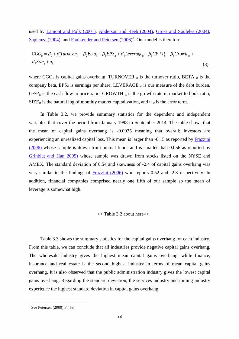
33

used by Lamont and Polk (2001), Anderson and Reeb (2004), Gross and Souleles (2004),

Sapienza (2004), and Faulkender and Petersen (2006)8. Our model is therefore

(3)

where CGOit is capital gains overhang, TURNOVER it is the turnover ratio, BETA it is the

company beta, EPSit is earnings per share, LEVERAGE it is our measure of the debt burden,

CF/Pit is the cash flow to price ratio, GROWTH it is the growth rate in market to book ratio,

SIZEit is the natural log of monthly market capitalization, and u it is the error term.

In Table 3.2, we provide summary statistics for the dependent and independent

variables that cover the period from January 1998 to September 2014. The table shows that

the mean of capital gains overhang is -0.0935 meaning that overall; investors are

experiencing an unrealized capital loss. This mean is larger than -0.15 as reported by Frazzini

(2006) whose sample is drawn from mutual funds and is smaller than 0.056 as reported by

Grinblat and Han 2005) whose sample was drawn from stocks listed on the NYSE and

AMEX. The standard deviation of 0.54 and skewness of -2.4 of capital gains overhang was

very similar to the findings of Frazzini (2006) who reports 0.52 and -2.3 respectively. In

addition, financial companies comprised nearly one fifth of our sample so the mean of

leverage is somewhat high.

<< Table 3.2 about here>>

Table 3.3 shows the summary statistics for the capital gains overhang for each industry.

From this table, we can conclude that all industries provide negative capital gains overhang.

The wholesale industry gives the highest mean capital gains overhang, while finance,

insurance and real estate is the second highest industry in terms of mean capital gains

overhang. It is also observed that the public administration industry gives the lowest capital

gains overhang. Regarding the standard deviation, the services industry and mining industry

experience the highest standard deviation in capital gains overhang.

8 See Petersen (2009) P.458

0 1 2 3 4 5 6

7

/it it it it it it it

it it

CGO Turnover Beta EPS Leverage CF P Growth

Size u

34

<< Table 3.3 about here>>

We report the sample correlation amongst the variables in Table 3.4. According to Alm

and Mason (2007), if the correlation coefficient amongst independent variables is less than

0.70, there should be no issues with high collinearity. According to this criterion, we do not

expect to have issues with collinearity since all our correlations are far less than 0.70. The

first and second highest correlation coefficients are between earnings per share and size

(0.40) and between cash flow to price and beta (0.26). The other correlation coefficients are

quite low, all less than 0.18. All the correlation coefficients are statistically significant at 1%

or 5% level except for the correlation between growth and turnover.


3.5- Empirical analysis

Our main empirical results are shown in Table 3.5. According to the rational investor

competitive market view, none of our variables should be systematically related to capital

gains overhang, yet all of them are significant at the 1% level. Moreover, the R-square of the

regression model is more than 20% and highly significant according to the F- Statistic.


We find very strong support for our first hypothesis. As expected, market liquidity

TURNOVER and systematic risk BETA are inversely related to capital gains overhang. Both

coefficients are significant at the 1% level. This is evidence of the activities of disposition

investors who are reluctant to realize capital losses. Evidently, with higher stock market

liquidity, disposition investors are realizing capital gains early yet are reluctant to realize

capital losses and so induce an inverse relation between stock market liquidity and unrealized

capital gains even though there is no rational reason why this relationship should exist.

35

We also find strong support for our second hypothesis. The four value irrelevant firm

characteristics that we hypothesize will attract demand from behaviourally biased investors

are indeed positively related to unrealized capital gains. All of these coefficients are

significant at the 1% level. Evidently, firms with larger earnings per share, growth, size and

leverage attract excess buying behaviour from behaviourally biased investors not

counteracted by more rational investors.

A fifth firm characteristic, corporate liquidity CF/P is inversely related to unrealized

capital gains and is also significant at the 1% level. This suggests that the disposition effect is

operative here rather than the irrational demand by behaviourally biased investors since

evidently; some firms with high corporate liquidity are inefficiently deploying resources

leading to losses that disposition investors are reluctant to realize. This finding is also

consistent with Lakonishok, Shleifer, and Vishny (1994) who find that investors tend to

overvalue growth stock "low cash flow to price", while they undervalue high cash flow to

price stocks.

Robustness checks

The main reason why we implement robustness check is to ensure regression estimates

are insensitive to different market conditions and are insensitive to different assumptions. The

first robustness check was conducted through running cross section regression for each year

to check the stability of the coefficients over time (see Table 3.6). Sixth further robustness

checks were conducted through splitting the whole sample into two subsamples, the first five

are based on median growth, median beta, median size, median turnover, before and after the

financial crisis and the sixth on the basis of capital gains versus losses. We first divided the

entire sample into two subsamples based on median growth in the market to book ratio. Then,

we ran the same model (1) (see Table 3.7). Similarly, the previous procedure is replicated in

beta, size and turnover in Tables 3.8, 3.9, and 3.10. To check the robustness of the relation to

different economic circumstances, the sample periods was split on the basis of occurring

before August 2007 or After August 2007 (see the subsamples in Table 3.11). Finally, we

divided the entire sample into two subsamples periods based on the capital gains overhang:

capital gains and capital losses (see Table 3.12). The main conclusion in Tables 3.6, 3.7, 3.8,

3.9, 3.10, 3.11 and 3.12 is that the relation is stable over time except BETA. This instable

relation between BETA and capital gains overhang can be attributed to the non-linear relation

between them. The findings are also robust to higher- and lower- growth stocks, higher- and

lower-beta stocks, higher- and lower-sized stocks, higher- and lower-liquidity stocks, boom

36

and recession conditions and also robust to capital gains and capital losses. There are three

differences between the main results and the robustness checks: the first difference lies in the

main conclusion (see Table 3.7) that there is positive significant relationship between growth

rate and capital gains overhang. But when we divided the whole sample according to growth

rate (high growth vs low growth) (see Table 3.7), we noticed that the relation between growth

rate and capital gains overhang became negative in the high growth subsample, indicating

that the disposition investor to some extent prefers high growth stocks. However, he does not

taste the extremely high growth stocks due to the high level of uncertainty that they represent.

From this point, we can see also that there is a nonlinear relationship between growth rate and

capital gains overhang. The second different story (see Table 3.12) is that we ran the panel

regression model (1) to the capital gains and capital losses separately. In the case of capital

gains the turnover coefficient became positive and significant at 10%, meaning that if the

disposition investor expects to earn capital gains, he pays little attention to the stock's trading

activity and likes to buy the higher-volume stocks rather than the lower-volume stocks, while

he is very much concerned about the trading activity when facing capital losses as the

turnover coefficient is highly significant in the capital losses subsample. The final different

story is that, we still find in capital gains subsample (see Table 3.12) that the sign of the beta

coefficient also becomes positive, referring to the fact that the disposition investors favour

high-beta stocks when facing gains to maximize their benefits. All other robustness tests are

quite consistent with the main conclusion.

Finally, we consider some subsamples statistics. The above median sized subsample of

"large sized companies" has a mean capital gains overhang of 0.05, while the smaller sized

"below median" mean subsample is -0.24. There is thus no size effect here and the difference

between the two subsamples is 0.29. However, the mean unrealized capital gains overhang on

the above median turnover subsample is -0.12, while it is -0.06 on the below median

turnover. Similarly, the below median subsample has a higher unrealized capital gains

overhang and the difference in unrealized capital gains overhang is 0.18.

3.6- Conclusion

In this study, we aimed to determine the main factors that might attract the disposition

investors to trade in, generating temporary price distortions. In doing so, we followed

Petersen (2009) methodology to attain efficient and unbiased standard errors in the context of

the panel regression models. The purpose of using the panel regression model is to describe

37

the time series and cross section behaviour of capital gains overhang. Turnover, firm beta,

EPS, leverage, cash flow to price, growth, and size were chosen. The relationships between

the capital gains overhang and turnover, beta and cash flow to price were negative, while it is

positive between the capital gains overhang and earnings to price, leverage, growth and size.

The conclusion introduced here is conformable with Lakonishok, Shleifer and Vishny (1994):

that, - firm characteristics are the main reason for irrationality and price distortion.

The main conclusion can be summarized as follows: there is strong evidence that

disposition investors believe that "good stocks are the stocks of good companies", especially

the strongest significant variables are, cash flow to price, growth and size, are firm

characteristics, while the turnover variable that is used as a proxy for market activity is far

less significant than firm characteristics mentioned above. The robustness checks were

implemented through running cross sectional regression year by year and through dividing

the whole sample on the basis of median growth, median size, median turnover, median beta,

before and after the financial crisis and capital gains and capital losses separately. In general,

the robustness tests support the main result.

The main implication for this paper is that the rational investors who are less

susceptible to cognitive errors can develop profitable trading strategies to benefit from the

temporary mispricing caused by the irrational investors. In this context, we would encourage

the rational investors to pay more attention to those good companies that attracted the

irrational investors and in turn, provides a higher capital gains overhang such as more

profitable firms, higher growth, higher levered firms, larger firms and firms with lower

corporate liquidity. Finally, it may be useful to make some recommendations for theory

development. Investigating other factors such as management efficiency, quality products,

innovation and social responsibility and replicating this research in other developed and

emerging markets would be interesting.

38

Tables of results

Table 3.1. A description of the variables

Variable Definition

Capital gains overhang The capital gains overhang is calculated as the

percentage difference between current prices and the

reference price.

t tt

t

P RPCGO

P

Turnover The turnover is a measure of shares monthly trading

volume divided by monthly shares outstanding as a

proxy for liquidity.

Company Beta A measure of systematic risk: The beta value is

determined by the CAPM for the past two years of

weekly data using S&P 500.

EPS Is the Earnings per share and computed as net income

available to common shareholders divided by the basic

weighted average shares outstanding. Sum of the most

recent 12 months (trailing 12 months).

Leverage A measure of the debt burden of a company. It is equal

to the ratio of debt to equity.

CF/P Is the ratio of cash flow to price.

The market to book ratio Is a proxy for growth.

The company Size Proxied by monthly market capitalization.

39

Table 3.2. Descriptive statistics

This table reports the descriptive statistics of the data. The capital gains overhang is (Pt-RPt)/Pt where Pt is the

stock price at the end of month t and RPt is the reference price calculated according to Grinblatt and Han (2005).

Turnover is measured monthly and is the trading volume divided by the number of shares outstanding. Beta is

the CAPM beta calculated over the previous two years using weekly data. EPS is the net income available to

common shareholders divided by the weighted average number of shares outstanding (trailing 12 months).

Leverage is calculated as the ratio of debt to equity. Cash flow to price CF/P is the ratio of cash flow per share

divided by the stock's price. The growth is the growth rate in a market to book ratio and computed as

1 1/ / / ( / ) 100t t tM B M B M B , when M/B is the market to book ratio. Size is the natural

logarithm of the market capitalization at the end of month t.

Variable

Mean Median Std. Dev. Min Max Skewness Obs

CGO

-0.093 0.062 0.547 -2.395 0.493 -2.394 422278

Turnover

0.008 0.006 0.009 0.000 0.040 2.148 422278

Beta

1.129 1.044 0.754 -0.310 3.205 0.595 422278

EPS

1.298 1.200 2.014 -4.280 7.240 0.231 415244

Leverage

2.793 1.329 3.715 0.109 16.823 2.211 410603

CF/P

0.123 0.093 0.100 0.012 0.520 2.053 367977

Growth (%) 0.528 0.000 12.776 -32.075 39.204 0.345 410846

Size (in

billions)

4.800 1.200 10.200 0.140 56.000 3.700 418730

40

Table 3.3. Summary statistics for capital gains overhang by industry

This table reports the capital gains overhang. The capital gains overhang = (Pt-RPt)/Pt. Pt is the stock price at the end of month t and RPt is the reference price calculated

according to Grinblatt and Han (2005). Using the first two digits of SIC codes, all stocks are assigned into ten industries as follows: Agriculture (01-09), Mining (10-14),

Construction (15-17), Manufacturing (20-39), Transportation and public utlity (40-49), Wholesale trade (50-51), Retail trade (52-59), Finance, Insurance and Real Estate

(60-67), Services (70-89), and Public Administration (91-99).

Industry Agriculture Mining Construction Manufacturing

Transportati

on and

Public Utility

Wholesale

Trade

Retail

Trade

Finance,

Insurance and

Real Estate

Services Public

Administration

Mean -.093 -0.115 -0.096 -0.110 -0.072 -0.0388 -0.060 -0.057 -0.136 -0.367

Std.

Dev 0.464 0.597 0.576 0.559 0.520 0.480 0.528 0.494 0.604 0.569

Min -2.395 -2.395 -2.395 -2.395 -2.395 -2.395 -2.395 -2.395 -2.395 -2.395

Max 0.493 0.493 0.493 0.493 0.493 0.493 0.493 0.493 0.493 0.493

Obs 631 17171 5273 163231 41334 11163 29618 91255 62536 66

41

Table 3.4. Correlation Matrix

Table 3.4 reports the correlation coefficients of the panel regression model. The dependent variable is a

capital gains overhang. The capital gains overhang = (Pt-RPt)/Pt. Pt is the stock price at the end of month t

and RPt is the reference price calculated according to Grinblatt and Han (2005). Turnover is measured by

monthly trading volume/ monthly shares outstanding. Beta is the CAPM beta calculated over the previous

two years using weekly data. EPS is computed as the net income available to common shareholders divided

by the basic weighted average shares outstanding (trailing 12 months). Leverage is the ratio of debt to

equity. CF/P is the ratio of the cash flow per share divided by the stock's price. The growth is the growth rate

in a market to book ratio and computed as 1 1/ / / ( / ) 100t t tM B M B M B , when M/B is the

market to book ratio. Size is the natural logarithm of the market capitalization at the end of month t.

Variable CGO Turnover Beta EPS Leverage CF/P Growth

M-B

Log size

CGO 1.00

Turnover -0.113 1.00

Beta -0.136 0.181 1.00

EPS 0.361 -0.078 - 0.168 1.00

Leverage -0.024 -0.078 0.004 0.039 1.00

CF/P -0.403 0.050 0.036 -0.085 0.263 1.00

Growth (%) 0.136 -0.001* 0.033 -0.035 -0.018 -0.054 1.00

Logsize 0.341 0.08 -0.112 0.402 0.039 -0.170 0.013 1.00

(*) denote significance at 10% and 5% otherwise

42

Table 3.5. Panel regression output

This table reports the coefficients of the panel regression model. The dependent variable is a capital gains

overhang. The capital gains overhang = (Pt-RPt)/Pt. Pt is the stock price at the end of month t and RPt is the

reference price calculated according to Grinblatt and Han (2005). Turnover is measured by monthly trading

volume/ monthly shares outstanding. Beta is the CAPM beta calculated over the previous two years using

weekly data. EPS is computed as the net income available to common shareholders divided by the basic

weighted average shares outstanding (trailing 12 months). Leverage is the ratio of debt to equity. CF/P is the

ratio of the cash flow per share divided by the stock's price. The growth is the growth rate in a market to

book ratio and computed as 1 1/ / / ( / ) 100t t tM B M B M B , when M/B is the market to book

ratio. Size is the natural logarithm of the market capitalization at the end of month t.

Variables

Coefficients

β t

Intercept -7.005

(0.195)

-35.92

Turnover -5.426

(0.259)

-20.94

Beta -0.032

(0.002)

-13.24

EPS 0.035

(0.002)

12.35

Leverage 0.015

(0.002)

7.62

CF/P -1.705

(0.056)

-35.60

Growth (%)

0.004

(0.000)

76.04

Size 0.341

(0.019)

37.09

R2

40.49

F-statitics

P- Value

115.37

(0.000)

Obs

351062

Figures in the parenthesis are robust standard errors

Significant at 1% level

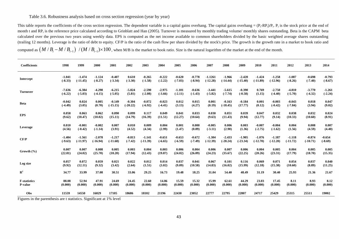
43

Table 3.6. Robustness analysis based on cross section regression (year by year)

This table reports the coefficients of the cross section regression. The dependent variable is a capital gains overhang. The capital gains overhang = (Pt-RPt)/Pt. Pt is the stock price at the end of

month t and RPt is the reference price calculated according to Grinblatt and Han (2005). Turnover is measured by monthly trading volume/ monthly shares outstanding. Beta is the CAPM beta

calculated over the previous two years using weekly data. EPS is computed as the net income available to common shareholders divided by the basic weighted average shares outstanding

(trailing 12 months). Leverage is the ratio of debt to equity. CF/P is the ratio of the cash flow per share divided by the stock's price. The growth is the growth rate in a market to book ratio and

computed as 1 1/ / / ( / ) 100t t tM B M B M B , when M/B is the market to book ratio. Size is the natural logarithm of the market at the end of the month.

Coefficients 1998 1999 2000 2001 2002 2003 2004 2005 2006 2007 2008 2009 2010 2011 2012 2013 2014

Intercept -1.041

(-8.33)

-1.474

(-11.45)

-1.124

(-8.27)

-0.407

(-3.34)

0.610

(-3.30)

-0.265

(-1.58)

-0.222

(-2.22)

-0.620

(-7.03)

-0.778

(-8.94)

-1.1261

(-12.28)

-1.966

(-14.44)

-2.420

(-15.40)

-1.424

(-11.89)

-1.258

(-12.96)

-1.087

(-8.26)

-0.698

(-7.40)

-0.793

(-8.67)

Turnover -7.636

(-6.22)

-6.384

(-5.03)

-4.298

(-4.15)

-6.215

(-5.05)

-5.824

(5.81)

-2.590

(-2.08)

-2.975

(-3.66)

-1.101

(-2.11)

-0.636

(-1.43)

-3.441

(-5.82)

-5.615

(-7.74)

-0.390

(-0.58)

0.769

(1.15)

-2.750

(-4.40)

-4.810

(-5.70)

-3.770

(-4.32)

-1.261

(-2.24)

Beta -0.042

(-4.49)

0.024

(3.05)

0.005

(0.70)

-0.149

(-15.15)

-0.304

(-20.22)

-0.072

(-6.92)

-0.023

(-4.41)

0.012

(3.13)

0.015

(4.27)

0.001

(0.19)

-0.163

(-18.45)

-0.184

(17.77)

0.001

(0.12)

-0.003

(-0.42)

-0.043

(-7.84)

0.018

(3.94)

0.047

(9.02)

EPS 0.058

(9.62)

0.063

(10.47)

0.062

(10.02)

0.090

(15.11)

0.099

(14.79)

0.117

(16.39)

0.049

(11.51)

0.041

(12.27)

0.033

(10.64)

0.030

(9.63)

0.051

(11.43)

0.039

(9.94)

0.047

(12.77)

0.032

(9.14)

0.038

(10.33)

0.032

(10.60)

0.024

(8.91)

Leverage 0.010

(4.56)

-0.001

(-0.42)

-0.002

(-1.14)

0.007

(3.91)

0.010

(4.52)

0.009

(4.34)

0.004

(2.99)

0.001

(1.47)

0.000

(0.09)

-0.005

(-3.11)

0.006

(2.90)

0.003

(1.36)

-0.007

(-2.75)

-0.004

(-1.62)

0.004

(1.56)

0.008

(4.59)

0.007

(4.40)

CF/P -1.404

(-9.63)

-1.561

(-11.97)

-2.078

(-16.94)

-1.217

(-11.68)

-0.813

(-7.42)

-1.141

(-11.39)

-0.651

(-6.65)

-0.653

(-6.59)

-0.672

(-7.49)

-1.304

(-12.39)

-2.433

(-28.24)

-1.905

(-23.34)

-1.076

(-12.70)

-1.187

(-12.20)

-1.118

(-11.72)

-0.874

(-10.71)

-0.654

(-8.69)

Growth (%) 0.007

(22.81)

0.007

(24.02)

0.008

(25.70)

0.005

(18.20)

0.003

(17.94)

0.004

(12.43)

0.003

(19.87)

0.006

(24.02)

0.004

(26.09)

0.006

(24.23)

0.007

(35.67)

0.006

(22.25)

0.004

(20.26)

0.005

(23.31)

0.004

(17.79)

0.005

(18.70)

0.005

(15.35)

Log size 0.057

(9.92)

0.072

(12.11)

0.059

(9.32)

0.021

(3.42)

0.022

(2.64)

0.012

(1.51)

0.014

(3.02)

0.037

(9.09)

0.041

(10.58)

0.067

(14.83)

0.101

(16.02)

0.116

(15.99)

0.069

(12.18)

0.071

(15.38)

0.054

(10.60)

0.037

(8.89)

0.040

(11.25)

R2 34.77 33.99 37.08 30.51 33.06 29.25 16.73 19.48 18.25 31.04 54.40 48.49 31.19 30.40 25.93 21.36 21.67

F-statistics

P-value

88.08

(0.000)

52.94

(0.000)

47.91

(0.000)

24.69

(0.000)

24.45

(0.000)

22.60

(0.000)

14.86

(0.000)

15.59

(0.000)

15.32

(0.000)

15.99

(0.000)

62.61

(0.000)

44.29

(0.000)

23.03

(0.000)

17.45

(0.000)

8.11

(0.000)

8.93

(0.000)

8.12

(0.000)

Obs 11559 14550 16029 17105 18686 18102 21196 22430 23052 22777 22795 22807 24717 25429 25315 25511 19002

Figures in the parenthesis are t statistics. Significant at 1% level

44

Table 3.7. Robustness analysis based on growth subsamples




volume/ monthly shares outstanding. Company beta is the CAPM beta calculated over the previous two years

using weekly data. EPS is computed as the net income available to common shareholders divided by the basic


ratio of the cash flow per share divided by the stock's price. The growth is the growth rate in a market to book

ratio and computed as 1 1/ / / ( / ) 100t t tM B M B M B , when M/B is the market to book ratio. Size

is the natural logarithm of the market capitalization at the end of month t.

Variables Above median growth Below median growth

β t β t

Intercept -6.111

(0.198)

-32.53 -7.274

(0.202)

-36.04

Turnover -5.00

(0.26)

-19.22 -4.707

(0.281)

-16.77

Beta -0.026

(0.000)

-14.62 -0.019

(0.003)

-6.63

EPS 0.026

(0.002)

13.08 0.022

(0.002)

10.21

Leverage 0.013

(0.002)

6.28 0.017

(0.002)

8.02

CF/P -1.557

(0.045)

-32.46 -1.656

(0.047)

-34.71

Growth (%) -0.002

(0.000)

-17.69 0.012

(0.000)

58.74

Size 0.304

(0.009)

34.21 0.355

(0.009)

37.25

R2 37.59

44.71

F-statitics

P- Value

40.82

(0.000)

85.64

(0.000)

Obs

179367 171696



45

Table 3.8. Robustness analysis based on beta subsamples










Variables Above median beta Below median beta

β t β t

Intercept -8.836

(0.243)

-36.30 -5.692

(0.190)

-30.02

Turnover -6.158

(0.331)

-18.57 -3.572

(0.236)

-15.12

Beta -0.0330

(0.004)

-8.13 -0.017

(0.003)

-5.40

EPS 0.023

(0.003)

8.61 0.022

(0.002)

11.44

Leverage 0.027

(0.002)

6.95 0.011

(0.002)

5.88

CF/P -1.832

(0.058)

-31.70 -1.379

(0.049)

-27.88

Growth (%) 0.004

(0.001)

45.82 0.005

(0.000)

55.37

Size 0.429

(0.015)

37.30 0.277

(0.009)

31.10

R2 45.72 34.51

F-statitics

P- Value

78.57

(0.000)

53.34

(0.000)

Obs 172777 178286



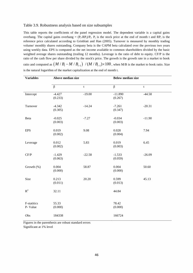
46

Table 3.9. Robustness analysis based on size subsamples










Variables Above median size Below median size

β t β t

Intercept -4.427

(0.233)

-19.00 -11.890

(0.267)

-44.58

Turnover -4.342

(0.305)

-14.24 -7.261

(0.347)

-20.31

Beta -0.025

(0.003)

-7.27 -0.034

(0.003)

-11.90

EPS 0.019

(0.002)

9.08 0.028

(0.004)

7.94

Leverage 0.012

(0.002)

5.83 0.019

(0.003)

6.45

CF/P -1.429

(0.063)

-22.58 -1.533

(0.059)

-26.09

Growth (%)

0.004

(0.000)

58.87 0.004

(0.000)

50.60

Size 0.213

(0.011)

20.20 0.599

(0.013)

45.13

R2 32.11 44.84

F-statitics

P- Value

55.33

(0.000)

78.42

(0.000)

Obs 184338 166724



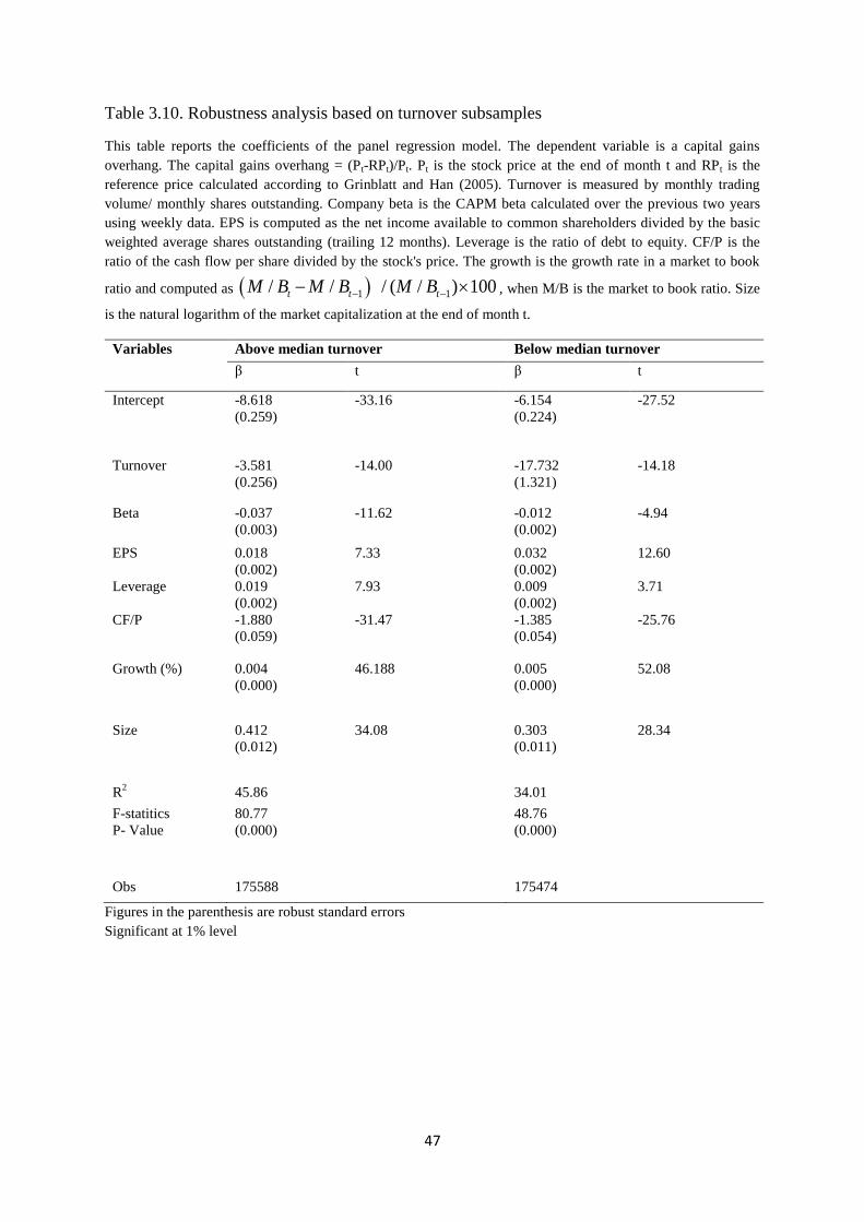
47

Table 3.10. Robustness analysis based on turnover subsamples










Variables Above median turnover Below median turnover

β t β t

Intercept -8.618

(0.259)

-33.16 -6.154

(0.224)

-27.52

Turnover -3.581

(0.256)

-14.00 -17.732

(1.321)

-14.18

Beta -0.037

(0.003)

-11.62 -0.012

(0.002)

-4.94

EPS 0.018

(0.002)

7.33 0.032

(0.002)

12.60

Leverage 0.019

(0.002)

7.93 0.009

(0.002)

3.71

CF/P -1.880

(0.059)

-31.47 -1.385

(0.054)

-25.76

Growth (%) 0.004

(0.000)

46.188 0.005

(0.000)

52.08

Size 0.412

(0.012)

34.08 0.303

(0.011)

28.34

R2 45.86 34.01

F-statitics

P- Value

80.77

(0.000)

48.76

(0.000)

Obs 175588 175474



48

Table 3.11. Robustness analysis based on before and after financial crisis subsamples










Variables Before August 2007 After August 2007

β t β t

Intercept -7.772

(0.245)

-31.67 -12.127

(0.293)

-41.39

Turnover -3.572

(0.363)

-9.83 -2.434

(0.245)

-9.94

Beta -0.015

(0.003)

-5.62 -0.017

(0.002)

-6.86

EPS 0.026

(0.000)

9.25 0.009

(0.002)

6.27

Leverage 0.019

(0.000)

6.49 0.011

(0.003)

3.65

CF/P -1.341

(0.062)

-21.72 -1.597

(0.059)

-27.23

Growth (%) 0.004

(0.000)

57.64 0.003

(0.000)

40.98

Size 0.374

(0.011)

32.36 0.569

(0.014)

41.32

R2

34.24 55.95

F-statitics

P- Value

52.7

(0.000)

106.95

(0.000)

Obs 175958 175105



49

Table 3.12. Robustness analysis based on capital gains/losses subsamples










Variables Capital gains Capital losses

β t β t

Intercept -1.395

(0.063)

-22.19 -8.901

(0.278)

-32.06

Turnover 0.128

(0.076)

1.68* -7.629

(0.347)

-21.96

Beta 0.009

(0.001)

11.85 -0.064

(0.004)

-17.73

EPS 0.003

(0.001)

4.18 0.023

(0.003)

9.08

Leverage 0.006

(0.001)

8.55 0.016

(0.002)

6.16

CF/P -0.284

(0.018)

-15.52 -1.435

(0.051)

-28.26

Growth (%) 0.002

(0.000)

75.12 0.003

(0.003)

45.85

Size 0.077

(0.003)

26.06 0.418

(0.013)

31.71

R2 14.44 37.40

F-statistics

P-value

52.37

(0.000)

57.66

(0.000)

Obs 214535 136575


(*) significant at 10% and 1% otherwise

50

Chapter Four

Revisiting disposition effect and momentum: A quantile

regression perspective

Abstract

Adopting quantile regression, we analyse the relationship between the unrealized capital

gains overhang and expected returns. The ability of the disposition effect to generate

momentum is also considered for the extreme expected return regions 0.05th

and 0.95th

. To do

so, we employ 450,617 observations belonging to 5176 US firms, covering a time span from

January 1998 to June 2015. Following the methodology of Grinblatt and Han (2005), we find

significant differences across various quantiles in terms of signs and magnitudes. These

findings indicate a nonlinear relationship between capital gains overhang and expected

returns since the impact of capital gains overhang as a proxy for disposition effect vary across

the expected return distribution. More precisely, the coefficients of capital gains overhang are

significantly positive and decline as the expected returns quantiles increase from the lowest

(0.05th

) to the median expected return quantiles. However, they become significantly negative

and rise with the increase in expected returns quantiles at the highest („above median‟)

expected returns quantiles. The findings also suggest that disposition effect is not a good

noisy proxy for inducing momentum at the lowest expected return quantile (0.05th

). However,

it seems interestingly to generate contrarian at the highest expected returns quantile (0.95th

).

Keywords Disposition Effect, Momentum, Quantile Regression; Grinblatt and Han (2005)

51

4.1- Introduction and Background

The disposition effect is the tendency of investors to realize gains too early and hold

losers too long. A main story is introduced by Grinblatt & Han (2005) who mentioned that

the story has two sides. First, when good news arrives to the stock market, it leads the stock

value to go up. Here the disposition investors sell the stock creating an excess supply

resulting in downward pressure on the stock prices. This causes a smaller initial price impact

and greater subsequent returns as the stock returns to its fundamental value. Second, when

bad news arrives, it causes a decline in the fundamental value. Here the disposition investors

prefer to hold the stock rather than selling it, leading to reduce the downward pressure on the

stock prices which hinder the bad news to fully incorporating into prices. In this case, the

subsequent returns will be smaller as the stock prices return to its fundamental value. In short,

this investor behaviour together with the absence of perfectly elasticity demand for stocks

generates return predictability and leads to under-reaction to news which eventually induces

momentum in returns.

Contradictory findings have been reached in the literature review on capital gains

overhang as a predictor for expected returns. These findings may be grouped into two main

categories: the first category claims that the unrealized capital gains overhang is a good

predictor for expected returns and there is a positive and significant relation between

expected returns and unrealized capital gains overhang. In this category, investors are shown

to follow the disposition behaviour. For instance, Grinblatt & Han (2005) develop new

framework depending on prospect theory and mental accounting to describe disposition

behaviour proxied by reference price and estimated by the following equation:

1

11

11

Tn

t t n t n t n

n

RP V V Pk

(1)

where Vt is the turnover ratio at date t, Pt-n is the probability that an investor bought a specific

stock at date t-n and still hold it. In the parentheses, the mathematical term is a weight, and all

weights total one. They support the positive relationship between unrealized capital gains

overhang and expected returns. Birru (2015) follows the procedures of Grinblatt and Han

(2005) to test the relation between capital gains overhang and expected returns using a

sample period from 1967 to 2011. Birru (2015) supports the positive relation between capital

52

gains overhang and expected returns either for the whole sample or February-December

subsample. Bhootra & Hur (2012) analyse the period from January 1980 to December 2005

and find result consistent with Grinblatt &Han (2005) since the top capital gains portfolio

gives the highest future returns per month, while the bottom capital gains portfolio provides

the lowest future returns. Bhootra & Hur (2012) also divide the sample into co-integrated and

non co-integrated subsamples and then they test the relation between unrealized capital gains

overhang and expected returns in each subsample. According to their finding, this relation is

positive for the two samples but stronger among non co-integrated stocks. Shumway & Wu

(2006) use data on 13,460 investors in the Chinese stock market and confirm that the

unrealized capital gains factor is a successful predictor for future return, and the relation

between them is statistically positive. Finally, Hur, Pritamani, & Sharma (2010) cover the

period 1980-2005 and demonstrate that the relation between capital gains overhang and

expected returns is significant and positive.

In contrast, the second category finds a negative relation between capital gains

overhang and future returns. In this category, investors follow the opposite behaviour of the

disposition effect through tending to sell losers too soon and holding winners too long. Kong,

Bai, & Wang (2014) employ firm-level data in the Chinese market from January 1998 to June

2013. They conclude that this relation between unrealized capital gains and future returns is

negative for the whole sample and for February to December subsample. Goetzmann &

Massa (2008) use daily data, follow Grinblatt and Han‟s methodology to estimate the

reference price and reach the conclusion that the disposition factor, at the market level and

stock level, is strongly and negatively related to future returns. Choe & Eom (2009) test the

relation between disposition effect and profits in the Korean futures market using account-

level data including all transactions from January 2003 to March 2005. Using cross-sectional

regression, they also discover negative relation between the disposition factor and account

returns.

The common drawback in most of the aforementioned studies, we claim they represent

the main streams in the literature review, is that they use a regression model based on the

conventional OLS technique. Therefore, these conflicting findings may reflect a nonlinear

relationship between the unrealized capital gains overhang and the expected returns.

The OLS technique is useful for estimating the average relationship of the dependent

and independent variables. However, it is not probably to work well if one is considering the

53

performance of extreme observations that represent the tails of a probability distribution

(Gowlland, Xiao, & Zeng, 2009). To simplify, the OLS produces the conditional mean and

relationship between the dependent variable and each independent variable is always

specified through only one estimate (Hallock, Madalozzo, & Reck, 2010). This means that if

the sensitivities or the coefficients vary across different expected return quantiles, then a

conventional OLS technique can be criticized for assuming homogeneity and concealing the

potential heterogeneity of the impact of the independent variables „X‟ on the dependent

variable „Y‟ across the distribution (Sula, 2011). Therefore, we use quantile regression to

describe how different are the relations between the capital gains overhang and the expected

returns across the conditional distribution of expected returns. In addition, the quantile

regression is robust to some common but undesirable characteristics in financial datasets such

as heteroscedasticity, skewness and heavy-tailed distribution (Pires, Pereiro, & Martins,

2015), (Cameron & Trivedi, 2010) and (Gowlland, Xiao, & Zeng, 2009).

This paper makes five contributions to the literature. As far as we know this paper is the

first to use quantile regression to investigate the determinants of capital gains overhang.

Providing a comprehensive picture of the relation between capital gains overhang and

expected returns by using quantile regression is the second contribution of the paper. The

third contribution is that we think we are the first to examine how linear the relationship

between capital gains overhang and expected returns is through testing the equality of

coefficients across different levels of expected returns. In other words, one motivation in our

research was that the shape of expected return and capital gains overhang relation was still

unknown since the OLS conventional technique does provide information about the possible

nonlinearity between the unrealized capital gains overhang and expected returns. The fourth

contribution is that we are the first, to our knowledge, to investigate the ability of the

disposition effect to induce momentum for the extreme regions (0.05th

and 0.95th

) of the

expected return distribution. Our sample, the Russell 3000 constituents, represents in many

ways the fifth contribution to the literature on the disposition effect and momentum: 1) we

are the first, to our knowledge, to include NASDAQ stocks, which made up one-fifth of our

sample. However, Grinblatt & Han (2005), Birru (2015), and Bhootra & Hur (2012) exclude

NASDAQ stocks from their samples even though NASDAQ contains plenty of leading stocks

especially the high-tech stocks, in the US stock market, which is characterized by high

volatility and high growth stocks; 2) Another advantage that improves the reliability of our

findings is that we free our sample of survivorship bias through updating the list of Russell

54

3000 index periodically; 3) depending on the Russell 3000 index which has the largest 3000

stocks makes our sample representative and properly captures investors‟ beliefs, while

including stocks that are excluded from the Russell 3000 index may lead to a spurious

findings since the prices would represent stale prices rather than investors‟ current beliefs.

The quantile regression findings explain that there is a heterogeneous impact on the

unrealized capital gains overhang of past returns on three different horizons. Fortunately, the

coefficients of short and intermediate past returns decline systematically with the increase in

unrealized capital gains quantiles, meaning that the momentum is stronger in the lowest

capital gains quantile and its strength reduces with the increase in capital gains quantiles.

Regarding the relation between the unrealized capital gains overhang and expected returns,

the coefficients are significantly positive and systematically decline with the increase in

expected returns quantiles from the lowest quantile (0.05th

) to the median. However, they are

significantly negative and systematically increase with the increase in the expected returns at

the above median quantiles, indicating that investors follow the disposition behaviour at the

median and below the median points, while they tend to engage in the opposite behaviour

above the median. Regarding the ability of disposition effect to generate momentum in

returns, at the lowest expected returns quantile (0.05th

), the disposition effect is not a good

noisy proxy for inducing the intermediate momentum. Finally, it interestingly generates

contrarian at the highest expected return quantile (0.95th

).

The reminder of this paper is organized as follows: the next section shows the

hypotheses development, Section 4.3 presents a brief summary of the quantile regression

model, section 4.4 describes our data, sample, and methodology, section 4.5 presents the

empirical results, section 4.6 demonstrates momentum and the disposition effect, and

conclusions are drawn in section 4.7.

4.2- Hypotheses Development

Jagadeesh and Titman (1993) define momentum, as past winners tend to overcome past

losers. Grinblatt and Han (2005) argue that relating past returns to capital gains overhang and

momentum trading is lucrative since stocks that experience a positive spread between market

prices and reference prices are expected to be future winners while stocks that experience

negative spread between market prices and reference prices are expected to be future losers.

In addition, we can proxy the unrealized capital gains facing disposition investors by using

55

past cumulative returns. The size of momentum mainly depends on the investors‟ reaction to

new information. Some writers suggest that investors respond in different way to good and

bad news. For instance, Epstein & Schneider (2008) claim that bad news is more effectual

than good news and, in turn, investors‟ reaction to bad news is more powerful. Kelsey,

Kozhan, & Pang, (2010) found various patterns in price persistence. They attribute this

asymmetric momentum to investors‟ different reactions to past winners and losers. These

different reactions are more probably to produce different relations between past returns and

capital gains overhang acrosss the unrealized capital gains distribution, which cannot be

proved by using the OLS technique of Grinblatt and Han (2005). In summary, our first

hypothesis can be stated as follows:

H1. Ceteris paribus, the relation between past returns over the three horizons and unrealized

capital gains is not uniform and varies across different quantiles.

Our second hypothesis addresses the relationship between capital gains overhang and

expected returns. Some studies indicate a positive relation between capital gains overhang

and expected returns Grinblatt and Han (2005), Birru (2015), Bhoora and Hur (2012) &

Shumway and Wu (2006). This positive relation means that investors adopt disposition

behaviour through realizing gains too soon and holding losers too long. Others discover a

negative relation between capital gains overhang and expected returns (Kong, Bai and Wang,

2014), (Goetzmann and Massa, 2008) & (Choe and Eom, 2009). This negative relation refers

to the converse of the disposition behaviour holding winners too long and realizing losses too

soon. Because all of the above studies use the conventional OLS technique, which gives no

information on possible nonlinearities, these conflicting findings may indicate a non-linear

relation between unrealized capital gains and expected returns. The second hypothesis can be

stated as follows:

H2. Ceteris paribus, the relation between expected returns and capital gains overhang is

nonlinear.

56

4.3- Quantile regression technique

In this section, we first discuss the conventional regression based on central tendency

including ordinary least square („OLS‟) and least absolute deviation („LAD‟). Then we

discuss the more advanced quantile regression model

4.3.1- OLS and LAD

Koenker and Basset (1978) devised a quantile regression technique to tackle the

shortcomings of traditional regression based on the conventional OLS technique. The

quantile regression runs multiple estimations at different data-points of the distribution of a

dependent variable „Y‟ rather than focusing only on the conditional mean (Davino, Furno, &

Vistocco, 2014). The basic regression model can adopt the following formula:

= .𝛽 + (2)

where y is the dependant variable, is the independent variable, u is the error term and 𝛽 is

the coefficient “slope”. i= 1, 2, 3,….N and t= 1, 2, 3,….. are the time and sample units

respectively. The traditional regression technique seeks to minimize the sum of squared error

(„SSE‟) using the following formula:

∑ )2

= ∑ - .𝛽)

2 (3)

However, the least absolute deviation (“LAD”) takes the following formula:

min ∑ = ∑ - . 𝛽| (4)

It is worth mentioning that 𝛽 refers to the conditional mean in the traditional regression

method and refers to the conditional median in the LAD technique and that both rely on one

central distribution tendency. This means that both techniques ignore the observations in the

two extremes of the distribution (Li & Hwang, 2011). To deal with this issue, the quantile

regression model should be used.

4.3.2- Quantile regression model

The quantile regression model is a developmental extension of the least square

conventional techniques. According to the quantile regression model, the conditional quantile

57

can be defined as a linear function of the independent variables. The basic formula of the

quantile regression model can be expressed as follows:

Y= 𝛽+ ε (5)

(YX= x) = (θ) and 0< θ < 1 (6)

where Y is the dependant variable, х is a matrix of independent variables, ε is the error term.

(YX= x) stands for the θth quantile of Y Conditional X =x. From Equation (6), we can

infer that the error term ε restricted by (∊∖X=x) = 0.

The quantile regression coefficient (θ) can be produced by solving the problem below:

∊ ∑ 𝛽 ∑ ) 𝛽 (7)

If the quantile is set as 50th

, then we deal with the median, and by going up from 0 to 1, we

pursue the distribution of Y, conditional on X. This should provide more information on the

relationship between the variables of interest (Koenker & Hallock, 2001)9.

Finally, it should be noted that segmenting the sample and employ OLS technique for

each subsample will produce a completely different results from the quantile regression since

the quantile regression uses all the data for each estimation procedure (Hallock, Madalozzo,

& Reck, 2010).

4.4- Data, sample and methodology description

We collect the monthly data of all constituents of the Russell 3000 index from January

1995 to June 2015. To deal with the expected survivorship bias, the list of companies was

updated every month. This leads the number of companies to increase substantially (about

5176 firms after removing all firms that have fewer than 36 observations). The data includes

closing price, trading volume and the number of outstanding shares to calculate the

unrealized capital gains overhang based on Grinblatt and Han (2005) as detailed in section

(4.1). However, we used the previous 36 months instead of 60 months to avoid losing a great

deal of data, meaning that the period from January 1998 to June 2015 was subjected to the

empirical analysis. We also used monthly rather that weekly data in calculating the unrealized

9 See Tsai (2012)

58

capital gains because our sample included a larger number of smaller stocks that that might

have been affected by thin trading if weekly data had been used.

The closing price is also used to calculate the stock return (r), the past cumulative

returns over the short horizon of the last three months (r-3:-1), the intermediate horizon

between the last four months and 12 months (r-12:-4) and the long horizon between the last 13

months and 36 months (r-36:-13). The monthly trading volume and number of shares

outstanding were collected in order to calculate the average turnover over the short horizon

(V-3:-1), the intermediate horizon (V-12:-4) and the long horizon (V-36:-13). Monthly market

capitalization was also collected and converted to a logarithm „log‟. Table 4.1 gives a detailed

description of all the dependent and independent variables.


On the methodological side, we compare the Fama and MacBeth (1973) two step

procedure with the quantile regression and we also control for the following: return effects,

proxied by cumulative return over the short, intermediate and long horizons; the return

premium effect of firm size proxied by logarithm of market capitalization, and the volume

effect measured by average monthly turnover over the past 12 months. We can formulate the

regression model as follows:

= + + + + + + g (8)

where rt is the monthly stock return. is cumulative monthly return from t- to t- . V

is the average monthly turnover over the previous 12 months. S is log (monthly market

capitalization. g is the capital gains overhang.

This quantile regression model is run at 5th

, 10th

, 25th

, 50th

, 75th

, 90th

and 95th

of the

expected returns quantiles. The bootstrapping resampling technique with 400 replications was

also run to estimate the standard errors. This bootstrapping helps to develop joint distribution

and develop F-statistics to examine the significant differences in the coefficients across the

conditional distribution quantiles. To address the shape of the relation between capital gains

overhang and expected returns and to test the heterogeneity of the capital gains overhang

59

impact across different levels of expected returns, we follow Koenker and Bassett (1982) and

Hendricks and Koenker (1991) who develop the following test

1 1

1 2 1 2( ) (H JH )( )n T T T TT (9)

We test the hypotheses H0: βT1= βT2 against H1:βT1≠ βT2 where Η-1

JH-1

is the

“sandwich” formula developed by Hendricks and Koenker (1991). If the null hypothesis is

not accepted, then we can confirm that there is a significant unequal coefficient across

various expected return distribution quantiles.10

In this case, we could say that the relation

between capital gains overhang and expected returns was nonlinear. Finally, in this paper we

tested the differences between coefficients or slopes at the θ against (1- θ) quantiles. For

instance, we compare the 0.05th

quantile versus the 0.95th

quantile, the 0.10th

quantile versus

the 0.90th

quantile and the 0.25th

quantile versus the 075th

quantile.


This section is divided into three subsections. The first of these discusses the

descriptive statistics, the second section highlights the determinants of capital gains overhang

and the third section focuses on the relation between capital gains overhang and expected

returns.

4.5.1– Descriptive statistics

In Table 4.2, we present the summary statistics for more than 454,400 stock-month

observations. We note that the capital gains overhang is negative (-0.08) with standard

deviation (0.48). However, the average returns in our sample is positive (0.01) with standard

deviation (0.11). We also report the summary for the 10th

percentile, median and 90th

percentile.


10 Hallock, K.F, & et.al.(2010). CEO pay for performance heterogeneity using quantile regression. The financial

Review, 45, 1-19

60

4.5.2- The cross sectional determinants of unrealized capital gains overhang

The first step in our analysis was to investigate the relation between capital gains

overhang and its determinants, including past cumulative returns over three different

horizons, past average turnover over three different horizons and size.

= + + + + + + + S (9)

where gt is capital gains overhang. is cumulative monthly return from t- to t- .

is average monthly turnover from t- to t- . Table 4.3 shows the correlation

matrices.


Table 4.4 compare the Fama- MacBeth regression based on the conventional OLS

technique with quantile regression at 0.05th

, 0.10th

, 0.25th

, 0.50th

, 0.75th

, 0.90th

, and 0.95th

quantiles. This Table shows the consistent results of the Fama-MacBeth with Grinblatt and

Han (2005), since there is a positive and significant relation between the unrealized capital

gains and past cumulative returns over the past three horizons and a significantly negative

relation between the unrealized capital gains and average turnover over the three different

horizons and finally a positive relation between unrealized capital gains and size.


The quantile regression findings support our first hypothesis in terms of the impact of

past returns over the three different horizons; Panel B shows significant differences

for and across all capital gains overhang quantiles, while the long-term

cumulative return explains the uniform impact in some quantiles and the

heterogeneous impact in others. Interestingly, the coefficients of short-term and intermediate

cumulative returns decline systematically as the capital gains overhang increases. These

systematic patterns indicate that the ability of past winners (losers) to generate unrealized

capital gains (losses) is higher in the lowest quantiles and declines with the increase in capital

gains quantiles. In other words, the momentum is stronger in the lowest quantiles on the short

61

and intermediate horizons. All the robustness checks in Tables 4.5, 4.6 and 4.7 support the

previous conclusions.




Regarding the relationship between average turnover and capital gains overhang, the

theory suggests a negative relation since the higher the turnover, the faster the reference price

converges to the market price. However, the data-points close to the upper and lower

extremes show surprising results especially the highest capital gains quantile (0.95th

). In this

quantile, the relation between capital gains overhang and average turnover in the short and

long- term is positive and significant in almost all cases either in the main analysis (see Table

4.4) or in all robustness checks (see Tables 4.5, 4.6 and 4.7). This result means that the higher

the turnover, the more slowly the reference price converges to the market price, eventually

creating larger unrealized capital gains. Finally, in the lowest capital gains quantile (0.05th

)

the average turnover behaves the same as it does in the highest quantile (0.95th

) on the short

and long- term.

Size is the last variable in this model. The quantile regression shows a conclusion

completely consistent with the theory since the relation between capital gains overhang and

size is positive across all quantiles and in all cases including all robustness checks except the

below median institutional ownership. This finding reflects that the giant companies produce

larger unrealized capital gains, probably because the past cumulative returns may not be able

to capture the past growth made by the giant companies. The quantile regression also

provides some useful insights into the relation between size and capital gains overhang. In the

main finding (see Table 4.4) and all robustness (see Tables 4.5, 4.6 and 4.7), the size

coefficients decline systematically with the increase in capital gains quantiles, suggesting that

the ability of large companies to generate greater unrealized capital gains and capture the past

growth declines with the increase in capital gains quantiles.

62

4.5.3- Expected returns, past returns and unrealized capital gains

The Fama-Macbeth regression based on OLS in Table 4.8 shows a strongly positive

and significant cross-section relation between expected returns and capital gains overhang at

1% significance level. This result is consistent with Grinblatt and Han (2005) and Birru

(2015). However, it is hard using the OLS technique to distinguish the impact of unrealized

capital gains on expected returns between more and less profitable stocks across the

distribution and in the extreme regions. Quantile regression can deal with this issue.


Table 4.15 and 4.16 provide a well-organized summary of the relation between

expected returns and unrealized capital gains across all quantiles including the whole sample,

the seasonality subsamples and all robustness checks. From these tables, we can observe that

the coefficients of capital gains overhang are significantly positive and decline as the

expected returns quantiles increase from the lowest to the median expected return quantiles

(below median and median data-points). However, they become significantly negative and

rise with the increase in expected returns quantiles at the highest („above median‟) expected

returns quantile. In Table 4.16, we compare the coefficients at θ against (1-θ) quantiles. F-

statistics indicate significant differences in the coefficients of unrealized capital gains across

various expected returns quantiles, meaning that the observed nonlinearities extracted from

the quantile regression confirm a significant difference in the impact of unrealized capital

gains across various levels of expected returns including the extremely lucrative and the

extremely unprofitable stocks. This conclusion provides a strong support to our second

hypothesis and asserts the nonlinear relation between unrealized capital gains and expected

returns. This conclusion provides some insights into the conflicting findings in the literature,

although confirming these conflicting findings might be attributed to the nonlinear

relationship between the two variables of interest. In sum, the irrational investors follow the

disposition behaviour of selling the winners too soon and holding losers too long at the

median and below median expected returns points, while they follow the converse pattern of

disposition behaviour at the above median expected returns points.


63


Finally, Tables 4.8, 4.9, 4.10, 4.11, 4.12, and 4.13, show strong persistence in the short-

term cumulative returns („ ‟) in all cases using either the whole sample or seasonal

subsamples or robustness checks subsamples across all quantiles. The main reason why we

implement robustness check is to ensure regression estimates are insensitive to different

market conditions and are insensitive to different assumptions. Fortunately, the coefficients

of short-term and long-term cumulative returns tend to go up systematically with the

increase in expected returns quantiles. However, the intermediate cumulative return shows

a systematic pattern in December only since it increases with the increase in expected returns

quantiles. Apart from December, there is robust evidence that the intermediate cumulative

returns go up systematically from the lowest expected returns quantile to the median point

and goes down systematically above the median to the highest expected returns quantile

(0.95th

).







4.6- Disposition effect and momentum

This section checks the ability of the disposition effect to drive intermediate

momentum. Grinblatt and Han (2005) conclude that the disposition effect alone can induce

the intermediate momentum effect described by Jagadeesh and Titman (1993) since the

intermediate momentum disappears once the unrealized capital gains overhang is controlled

for. Birru (2015) doubts the ability of the disposition effect alone to induce momentum and

demonstrate that the momentum is too complicated to be generated by disposition effect

alone. Shumway & Wu (2006) also produce evidence that the disposition effect drives

64

momentum using account-level data. Muga & Santamaría (2009) study the momentum and

disposition effect in the spanish stock market. They recommend combining under-reaction

theory based on the disposition effect with over-reaction theory when explaining the

momentum effect since under-reaction and disposition successfully induce momentum in

down markets, while over-reaction does the same in up markets. Hur, Pritamani, & Sharma

(2010) relate the ability of the disposition effect to induce momentum with the proportional

representation of individual investors. They believe that the higher the number of individual

investors, the stronger the ability of the disposition effect to induce momentum. Despite the

practical importance of the highest gains and the highest losses stocks, none in the literature,

to our knowledge, attempts to check the sources of momentum for the most extreme expected

returns quantiles (0.05th

and 0.95th

).

In this paper, we focus on the extreme expected return regions (0.05th

and 0.95th

). From

a practical point of view, the behaviour of the extreme regions attracts the particular attention

of risk managers as well as investors since they represent the stocks with the highest gains

and the highest losses (Nath & Brooks, 2015). In addition, the OLS conventional technique

used by Grinblatt and Han (2005) and the other previous studies is not only not useful for

understanding the behaviour of the extreme regions but also very sensitive to outliers and

ignores the behaviours of data-points which are very far from the mean (Gowlland, Xiao and

Zeng, 2009) & (Naifar, 2015). Moreover, the use of the OLS technique always leads to

ignoring the information on the tails of a probability distribution (Chiang, Li, & Tan, 2010).

The quantile regression, however, is more effective in dealing with outliers and heavy-tailed

distributions (Pires, Pereira, & Martins, 2015). We conclude from the above discussion that

the uniqueness of the extreme regions justifies examining them alone.

Following Grinblatt and Han (2005), we proceed to examine in three stages the ability

of the disposition effect to drive momentum by running Fama-MacBeth (1973) two-step

procedures and quantile regression with and without capital gains overhang as follows:

= + + + + (10)

= + + + + + (11)

= + + + + + + g (12)

65

where rt is the monthly stock return. is cumulative monthly return from t- to t- . V

is the average monthly turnover over the previous 12 months. S is log (monthly market

capitalization. g is capital gains overhang.

In this part, we were satisfied by presenting only the intermediate cumulative return

(„ ‟) from the model 10 and model 11 outputs because it is the variable of interest, and other

regression outputs were not needed. Table 4.14 includes the intermediate cumulative returns

for the three regressions („before and after controlling for the unrealized capital gains‟) to

facilitate reading and comparing the coefficients.


Focusing on the lowest (0.05th

) and highest (0.95th

) expected returns quantiles, it is

worth noting that the intermediate cumulative return is strongly positive and significant in the

lowest expected return quantile (0.05th

) before the unrealized capital gains overhang is

controlled for. Once we added the unrealized capital gains overhang, most of the intermediate

cumulative returns coefficients turned significantly negative, meaning that the disposition

effect was not a good noisy proxy to generate momentum at the lowest expected return

quantile (0.05th

). This finding is robust to institutional ownership, leverage and size.

However, most of the highest expected returns quantiles (0.95th

) have strongly significant and

negative intermediate cumulative returns, which means that there is a reversal in return. In

other words, the intermediate momentum of Jagadeesh and Titman (1993) is not profitable in

the highest expected returns quantile (0.95th

). Interestingly, when we control for unrealized

capital gains, almost all the negative coefficients, except below median institutional

ownership and large size subsamples, became insignificant. This conclusion means that the

opposite behaviour of disposition can successfully drive intermediate contrarian rather than

momentum at the highest expected return quantile (0.95th

) in all cases except the above

median size and below median institutional ownership stocks since the contrarian disappears

when we control for unrealized capital gains. This occurs, when stocks experience significant

capital gains and the investors tend to be risk lovers because the current gains protect them

against future losses and, the prices are usually high. As a result, the investors look forward

to lower expected returns. However, if the stocks experience unrealized capital losses and the

investors are more risk-averse, the investors look forward to higher expected returns.

66

4.7- Conclusion

In this paper, we have tried to extend the literature through using an unconventional

quantile regression technique since previous studies on the relation between expected returns

and capital gains overhang provide mixed findings. One important conclusion in our paper is

that these contradictions in the literature can, to some extent, be attributed to the nonlinear

relationship between the unrealized capital gains overhang and expected returns. Second, the

disposition-prone investors follow disposition behaviour at the below median and median

expected returns quantiles but they follow the converse behaviour at the above median

expected returns quantiles. Our findings also explain that the disposition effect is not a good

noisy proxy for inducing intermediate momentum at the lowest expected returns quantile

(0.05th

). Therefore, it would be of interest for future research to examine the other sources of

momentum such as the risk-based explanation at the lowest expected return quantile (0.05th

).

At the highest expected returns quantile (0.95th

) the opposite disposition effect contributes

entirely in generating contrarian rather than momentum. These findings are robust to

institutional ownership, leverage and size.

In sum, we can conclude that the OLS estimates that neglect the embodied

heterogeneity in the stocks can produce incorrect conclusions. Finally, this paper suggests

several research points for future consideration, such as using the quantile regression to

investigate the relation between the unrealized capital gains overhang and expected returns,

and the ability of disposition effect to generate momentum in returns in a range of developed

and emerging markets.

67

Tables of results

Table 4.1. Description of the independent variables.

Variable Definition

Capital gains overhang The capital gains overhang is calculated as the

percentage difference between current prices and

the reference price.

t tt

t

P RPCGO

P

Where Pt is the closing price at time t and RPt is

reference price calculated based on equation (1).

Stock return The change rate in monthly closing price

=

Where is the closing price at month t and

is the closing price at month t-1.

r-3:-1 The past cumulative returns over the short horizon

of the last three months.

r-12:-4 The intermediate horizon between the last four

months and 12 months.

r-36:-13 The long horizon between the last 13 months and

36 months.

V-3:-1 The average turnover over the short horizon of the

last three months.

V-12:-4 The average turnover between the last four months

and 12 months.

V-36:-13 The average turnover between the last 13 months

and 36 months.

V A proxy for volume effect and computed as

average monthly turnover over the past 12 months.

Institutional Ownership The percentage ratio of freely traded shares held

by institutions to the number of Float Shares

Outstanding.

Leverage A measure of the debt burden of a company. It is

equal to the monthly ratio of debt to equity

The company Size (S) Proxied by monthly market capitalization.

68

Table 4.2. Summary statistics

This table demonstrates various descriptive statistics such as mean, median, standard deviations, minimum,

maximum and skewness for capital gains overhang g, expected returns r, past returns over three horizons r-3:-1, r-

12:-4 and r-36:-13, Size S and average volume V.

Variables

Mean Median Std.

Dev.

Min Max Skew 10th

Pct.

90th

Pct.

Obs

g

-0.0772 0.0633 0.4846 -1.8358 0.4454 -2.0530 -0.6490 0.3320 454432

r

0.0096 0.0086 0.1072 -0.2316 0.2651 0.0911 -0.1251 0.1446 454467

r-3:-1

0.0293 0.0253 0.1919 -0.3850 0.4931 0.1734 -0.2136 0.2728 454474

r-12:-4

0.0895 0.0692 0.3469 -0.5831 0.9948 0.4692 -0.3417 0.5341 454474

r-36:-13

0.2569 0.1789 0.6226 -0.7460 2.0176 0.8622 -0.4776 1.0745 454474

S

21.1036 20.9056 1.4325 18.8261 24.3868 0.5002 19.3370 23.2082 450658

V

0.0086 0.0066 0.0071 0.0008 0.0308 1.4827 0.0018 0.0250 454474

69

Table 4.3. Correlation matrices and Heteroscedasticity

where g is capital gains overhang; r-t1:-t2 = cumulative returns from month t-t1 through t-t2 computed over three

past return horizons; r-t1:-t2; V-t1:-t2 = average monthly turnover from t-t1 through t-t2; V= average monthly

turnover ratio (share volume divided by the number of shares outstanding) over the previous 12 month. S =

natural logarithm of monthly market capitalization; return is the month-t return.

Panel A correlation matrix for the determinants of capital gains overhang

Variable

CGO

r-3:-1

r-12:-4

r-36:-13

v-3:-1

v-12:-4

v-36:-13

S

g 1.00

r-3:-1

0.39 1.00

r-12:-4

0.59 0.53 1.00

r-36:13

0.66 0.30 0.52 1.00

v-3:-1

-0.14 -0.03 -0.04 -0.01 1.00

v-12:-4

-0.16 -0.03 -0.06 -0.04 0.87 1.00

v-36:13

-0.17 -0.02 -0.04 -0.07 0.76 0.88 1.00

S

0.35 0.09 0.17 0.28 0.07 0.06 0.05 1.00

Panel B correlation matrix for expected returns, past returns and capital gains overhang

Variable

return

r-3:-1

r-12:-4

r-36:-13

V

S

CGO

return 1.00

r-3:-1

0.54 1.00

r-12:-4

0.30 0.53 1.00

r-36:-13

0.18 0.30 0.52 1.00

V

-0.01 -0.03 -0.05 -0.05 1.00

S

0.05 0.09 0.17 0.28 0.06 1.00

g

0.24 0.39 0.59 0.66 -0.17 0.35 1.00

Significance level at 5%

Panel C: Heteroscedasticity (Breusch-Pagan test)

Model Model one Model two Model three Model four

P- Value 0.000 0.000 0.000 0.000

These results indicate that all models suffer from Heteroscedasticity which can be taken as a justification for

using quantile regression because quantile regression is robust to heteroscedastictic data.

70

Table 4.4. Determinants of capital gains overhang: Fama-MacBeth and Quantile regression

Panel A: Determinants of capital gains overhang: Fama-MacBeth and Quantile regression

= + + + + + + + S

where g is capital gains overhang; r-t1:-t2 = cumulative returns from month t-t1 through t-t2 computed over

three past return horizons; r-t1:-t2; V-t1:-t2 = average monthly turnover from t-t1 through t-t2; S = natural

logarithm of monthly market capitalization.

Explanatory

Variables

Fama-

MacBeth

0.05

0.10

0.25

0.50

0.75

0.90

0.95

-1.2126

(-30.98)

-6.2631

(-151.13)

-3.7825

(-177.15)

-1.6731

(-179.18)

-0.6914

(-155.05)

-0.2888

(-87.95)

-0.0343

(-8.96)

0.1185

(27.08)

0.2889

(23.37)

0.5066

(26.10)

0.3899

(33.13)

0.2571

(47.81)

0.1985

(65.15)

0.1718

(79.36)

0.1518

(71.05)

0.1467

(52.87)

0.3786

(33.11)

0.3984

(31.27)

0.3415

(44.88)

0.2976

(73.71)

0.2754

(118.26)

0.2589

(156.74)

0.2448

(136.15)

0.2338

(109.94)

0.3213

(33.37)

0.1641

(31.59)

0.1909

(50.67)

0.2209

(100.13)

0.2236

(154.69)

0.2126

(198.30)

0.1921

(196.35)

0.1707

(160.24)

-1.7863

(-4.38)

0.0017

(1.80) *

0.0012

(1.75) *

0.0002

(1.04)

0.0002

(1.49)

0.0003

(3.96)

0.0004

(4.62)

0.0004

(3.36)

-1.6324

(-2.51)

0.0008

(0.56)

0.0005

(0.48)

0.0005

(1.97)

0.0000

(0.21)

-0.0004

(-3.73)

-0.0008

(-5.37)

-0.0011

(-6.11)

-6.3299

(-12.41)

-0.0040

(-4.23)

-0.0027

(-3.79)

-0.0008

(-5.18)

-0.0002

(-1.55)

0.0003

(5.11)

0.0008

(8.57)

0.0012

(13.05)

0.0538

(31.51)

0.2435

(145.65)

0.1489

(166.39)

0.0674

(162.73)

0.0296

(146.02)

0.0151

(98.14)

0.0064

(37.00)

0.0014

(7.34)

R2

60.40 15.12 16.16 18.67 22.18 25.63 27.31 27.11

Panel B: Tests of the equality-of-slope estimates across quantiles

Variables

Quantiles

0.05 vs. 0.95 0.10 vs. 0.90 0.25 vs. 0.75

F-statistics P-value F-statistics P-value F-statistics P-value

353.75 (0.0000) 449.86 (0.0000) 378.40 (0.0000)

179.76 (0.0000) 198.52 (0.0000) 150.84 (0.0000)

1.77 (0.1839) 0.12 (0.7248) 28.45 (0.0000)

1.73 (0.1878) 1.19 (0.2743) 0.35 (0.5546)

1.75 (0.1853) 1.58 (0.2088) 15.19 (0.0001)

30.63 (0.0000) 24.92 (0.0000) 60.64 (0.0000)

20862.43 (0.0000) 26125.98 (0.0000) 19139.35 (0.0000)

Figures in brackets are t-statistics. Standard errors are corrected by bootstrapping for quantile regression (400 runs)

and corrected by Newey-West for Fama-MacBeth. R2 for Fama-MacBeth is an average R

2, however it is Pseudo R

2

for Quantile regression. (*) Significance at 10% and 5% otherwise.

71

Table 4.5. Determinants of Capital gains overhang: Robustness analysis based on institutional ownership subsamples

= + + + + + + + S

where g is capital gains overhang; r-t1:-t2 = cumulative returns from month t-t1 through t-t2 computed over three past return horizons; r-t1:-t2; V-t1:-t2 = average monthly turnover from t-t1

through t-t2; S = natural logarithm of monthly market capitalization.

Above median institutional ownership below median institutional ownership

Coefficients

Fama -

MacBeth

0.05

0.10

0.25

0.50

0.75

0.90

0.95

Fama -

MacBeth

0.05

0.10

0.25

0.50

0.75

0.90

0.95

-1.0901

(-28.48)

-5.7405

(-112.42)

-3.5719

(-129.23)

-1.6788

(-137.31)

-0.7636

(-121.58)

-0.3631

(-70.04)

-0.0866

(-14.67)

0.0609

(9.25)

-1.2090

(-30.31)

-7.4464

(-103.92)

-4.2877

(-131.93)

-1.7434

(-135.30)

-0.6551

(-111.86)

-0.2207

(-51.82)

0.0261

(5.20)

0.1797

(27.68)

0.2590

(21.82)

0.3916

(16.69)

0.3148

(23.47)

0.2241

(34.70)

0.1863

(50.40)

0.1605

(55.57)

0.1417

(52.39)

0.1368

(38.70)

0.3073

(21.91)

0.6161

(16.47)

0.4558

(21.22)

0.2939

(31.24)

0.2103

(39.19)

0.1846

(51.69)

0.1647

(40.74)

0.1584

(30.48)

0.3440

(30.97)

0.3313

(28.71)

0.2953

(40.87)

0.2690

(64.61)

0.2554

(94.74)

0.2421

(118.01)

0.2297

(109.72)

0.2203

(85.38)

0.4080

(32.39)

0.4521

(18.71)

0.3961

(29.63)

0.3299

(46.33)

0.2994

(71.85)

0.2773

(101.45)

0.2643

(95.02)

0.2520

(76.68)

0.2835

(32.99)

0.1460

(30.33)

0.1708

(50.87)

0.1953

(83.02)

0.1991

(123.48)

0.1934

(154.97)

0.1794

(150.40)

0.1637

(130.82)

0.3679

(33.28)

0.1659

(15.45)

0.2082

(29.45)

0.2543

(58.33)

0.2555

(97.96)

0.2360

(118.80)

0.2044

(120.77)

0.1745

(82.99)

-1.5006 (-3.58)

-0.0006 (-2.33)

-0.0004 (-1.95)*

0.0001 (0.24)

0.0002 (1.07)

0.0001 (0.76)

0.0001 (0.80)

0.0000 (0.01)

-2.2312 (-4.49)

0.0030 (2.76)

0.0019 (2.51)

0.0002 (0.74)

0.0003 (2.27)

0.0004 (3.97)

0.0006 (6.45)

0.0008 (5.29)

-2.0000

(-3.02)

-0.0004

(-1.38)

-0.0003

(-1.09)

-0.0001

(-0.56)

-0.0003

(-1.65)

-0.0003

(-1.44)

-0.0006

(-2.55)

-0.0007

(-2.44)

-1.0557

(-1.37)

-0.0000

(-0.01)

0.0002

(0.23)

0.0009

(2.04)

0.0002

(0.99)

-0.0005

(-3.85)

-0.0009

(-5.16)

-0.0015

(-7.44)

-5.3234

(-9.41)

0.0009

(10.43)

0.0005

(5.28)

0.0001

(1.31)

0.0002

(2.67)

0.0004

(2.35)

0.0008

(7.01)

0.0012

(6.05)

-8.0421

(-13.81)

-0.0045

(-3.36)

-0.0033

(-4.47)

-0.0014

(-5.37)

-0.0005

(-4.00)

0.0004

(4.93)

0.0008

(6.42)

0.0013

(13.22)

0.0492 (29.47)

0.2309 (106.98)

0.1450 (121.31)

0.0698 (128.16)

0.0340 (119.08)

0.0194 (81.35)

0.0096 (35.35)

0.0046 (15.32)

0.0527 (30.57)

0.2857 (101.00)

0.1658 (125.33)

0.0684 (123.16)

0.0267 (101.72)

0.0109 (55.12)

0.0028 (12.37)

-0.0019 (-6.73)

R2

60.38 18.90 20.12 23.20 27.22 30.50 32.10 31.95 61.65 13.32 14.18 16.12 18.79 21.87 23.53 23.32


Figures in brackets are t-statistics. Standard errors are corrected by bootstrapping for quantile regression (400 runs) and corrected by Newey-West for Fama-MacBeth.

R2 for Fama and MacBeth is an average R


2 for Quantile regression. (*) Significance at 10% and 5% otherwise.

Below median institutional ownership

Variables

Quantiles

0.05 vs. 0.95 0.10 vs. 0.90 0.25 vs. 0.75


156.09 (0.0000) 205.59 (0.0000) 202.78 (0.0000)

72.55 (0.0000) 109.58 (0.0000) 89.07 (0.0000)

0.73 (0.3942) 0.35 (0.5550) 35.71 (0.0000)

3.78 (0.0517)* 3.14 (0.0763)* 0.21 (0.6445)

0.53 (0.4666) 1.01 (0.3144) 11.83 (0.0006)

19.22 (0.0000) 32.67 (0.0000) 57.10 (0.0000)

10521.31 (0.0000) 16214.41 (0.0000) 14428.61 (0.0000)

Above median Institutional ownership

Variables

Quantiles

0.05 vs. 0.95 0.10 vs. 0.90 0.25 vs. 0.75


121.95 (0.0000) 185.70 (0.0000) 147.68 (0.0000)

99.17 (0.0000) 97.55 (0.0000) 72.85 (0.0000)

15.11 (0.0001) 8.41 (0.0037) 1.39 (0.2390)

3.83 (0.0504)* 4.62 (0.0317) 0.07 (0.7892)

0.56 (0.4561) 0.85 (0.3577) 0.30 (0.5835)

1.56 (0.2122) 5.05 (0.0246) 1.92 (0.1660)

10844.25 (0.0000) 12963.84 (0.0000) 10539.38 (0.0000)

72

Table 4.6. Determinants of Capital gains overhang: Robustness analysis based on leverage subsamples

= + + + + + + + S

where g is capital gains overhang; r-t1:-t2 = cumulative returns from month t-t1 through t-t2 computed over three past return horizons; r-t1:-t2; V-t1:-t2 = average monthly turnover from t-t1

through t-t2; S = natural logarithm of monthly market capitalization.

Above median Leverage Below median Leverage

Explanatory

Variables

Fama -

MacBeth

0.05

0.10

0.25

0.50

0.75

0.90

0.95

Fama -

MacBeth

0.05

0.10

0.25

0.50

0.75

0.90

0.95

-1.2241 (-26.82)

-7.2931 (-102.42)

-4.2155 (-105.53)

-1.7050 (-123.23)

-0.6510 (-116.09)

-0.27 (-58.71)

-0.0375 (-7.31)

0.1139 (18.35)

-1.2111 (-34.90)

-5.3972 (-114.61)

-3.4387 (-125.88)

-1.6568 (-130.71)

-0.7525 (-107.56)

-0.3320 (-64.73)

-0.0538 (-8.56)

0.1012 (15.89)

0.2983

(21.25)

0.5130

(17.61)

0.3659

(20.18)

0.2373

(27.99)

0.1859

(39.94)

0.1645

(44.13)

0.1471

(41.71)

0.1449

(32.93)

0.2840

(22.46)

0.5309

(21.31)

0.4108

(30.49)

0.2787

(40.58)

0.2093

(52.07)

0.1770

(63.48)

0.1546

(51.82)

0.1491

(35.16)

0.3837

(33.24)

0.4010

(22.53)

0.3404

(27.92)

0.2868

(47.38)

0.2678

(73.05)

0.2566

(94.38)

0.2447

(95.05)

0.2330

(74.56)

0.3768

(30.93)

0.3927

(29.83)

0.3527

(45.53)

0.3069

(69.91)

0.2813

(99.98)

0.2607

(121.22)

0.2465

(107.80)

0.2351

(97.71)

0.3377 (31.69)

0.2231 (28.78)

0.2398 (42.54)

0.2575 (85.95)

0.2494 (127.54)

0.2321 (157.85)

0.2063 (130.47)

0.1810 (104.03)

0.3040 (33.28)

0.1158 (15.22)

0.1498 (30.64)

0.1888 (66.66)

0.2003 (107.15)

0.1953 (125.98)

0.1785 (118.94)

0.1611 (104.49)

-2.6433

(-5.32)

0.0020

(1.75)*

0.0009

(1.19)

0.0000

(0.06)

0.0001

(1.12)

0.0003

(4.37)

0.0005

(5.87)

0.0001

(3.75)

-0.8526

(-2.14)

0.0015

(0.88)

0.0019

(2.05)

0.0005

(1.33)

0.0002

(1.12)

0.0003

(1.97)

0.0005

(3.18)

0.0007

(3.22)

-2.1620

(-2.86)

-0.0000

(-0.04)

0.0011

(0.83)

0.0006

(1.68) *

0.0001

(0.83)

-0.0005

(-3.48)

-0.0009

(-7.87)

-0.0006

(-4.99)

-0.7337

(-1.12)

0.0002

(0.05)

-0.0008

(-0.46)

0.0003

(0.56)

-0.0001

(-0.71)

-0.0006

(-2.60)

-0.0012

(-4.56)

-0.0015

(-6.01)

-6.1900 (-11.41)

-0.0034 (-2.65)

-0.0031 (-3.46)

-0.0008 (-3.65)

-0.0003 (-3.16)

0.0003 (3.63)

0.0007 (10.22)

0.0010 (8.25)

-7.3536 (-12.43)

-0.0028 (-1.92)

-0.0016 (-1.58)

-0.0007 (-2.26)

0.0002 (2.27)

0.0007 (4.37)

0.0013 (7.38)

0.0015 (11.07)

0.0542

(27.25)

0.2851

(97.80)

0.1664

(100.40)

0.0682

(113.59)

0.0273

(108.86)

0.0136

(63.93)

0.0061

(26.31)

0.0009

(4.47)

0.0542

(35.66)

0.2085

(107.07)

0.1350

(115.53)

0.0672

(118.55)

0.0328

(101.57)

0.0176

(72.17)

0.0078

(26.23)

0.0027

(8.91) R2

60.61 15.13 15.41 17.06 20.10 23.47 25.15 24.99 60.90 16.32 17.95 21.07 24.96 28.35 29.84 29.47





2 for Quantile regression. (*) Significance at 10% and 5% otherwise

Below median leverage

Variables

Quantiles

0.05 vs. 0.95 0.10 vs. 0.90 0.25 vs. 0.75


241.62 (0.0000) 387.34 (0.0000) 303.72 (0.0000)

150.49 (0.0000) 209.34 (0.0000) 175.68 (0.0000)

37.29 (0.0000) 43.35 (0.0000) 10.89 (0.0010)

0.21 (0.6502) 2.46 (0.1169) 0.17 (0.6814)

0.32 (0.5689) 0.03 (0.8550) 3.23 (0.0723)*

8.88 (0.0029) 8.27 (0.0040) 20.12 (0.0000)

11139.65 (0.0000) 12235 (0.0000) 9369.66 (0.0000)

Above median Leverage

Variables

Quantiles

0.05 vs. 0.95 0.10 vs. 0.90 0.25 vs. 0.75


160.85 (0.0000) 159.09 (0.0000) 112.12 (0.0000)

95.13 (0.0000) 70.35 (0.0000) 44.66 (0.0000)

31.86 (0.0000) 43.36 (0.0000) 142.98 (0.0000)

1.55 (0.2133) 0.34 (0.5576) 2.51 (0.1129)

0.24 (0.6279) 2.40 (0.1214) 10.32 (0.0013)

11.35 (0.0008) 18.06 (0.0000) 28.38 (0.0000)

9540.41 (0.0000) 9543.94 (0.0000) 9893.68 (0.0000)

73

Table 4.7. Determinants of Capital gains overhang: Robustness analysis based on size subsamples

= + + + + + + + S

where g is capital gains overhang; r-t1:-t2 = cumulative returns from month t-t1 through t-t2 computed over three past return horizons; r-t1:-t2; V-t1:-t2 = average monthly turnover from t-t1 through t-t2; S =

natural logarithm of monthly market capitalization.






Above median size Below median size

Explanatory

Variables

Fama -

MacBeth

0.05

0.10

0.25

0.50

0.75

0.90

0.95

Fama -

MacBeth

0.05

0.10

0.25

0.50

0.75

0.90

0.95

-0.3684

(-18.03)

-2.3130

(-58.37)

-1.4017

(-66.29)

-0.6135

(-63.03)

-0.2567

(-49.63)

-0.0787

(-17.30)

0.0539

(9.40)

0.1346

(21.69)

-3.4445

(-47.60)

-32.6994

(-67.20)

-18.8849

(-89.90)

-7.5017

(-100.70)

-2.7913

(-91.6)

-1.0659

(-63.20)

-0.4919

(-25.30)

-0.2192

(-8.90)

0.2234

(20.08)

0.3762

(22.68)

0.3051

(27.30)

0.2303

(40.10)

0.1924

(55.54)

0.1600

(55.20)

0.1329

(48.81)

0.1213

(35.81)

0.3140

(22.00)

0.4632

(19.30)

0.3631

(23.50)

0.2703

(33.70)

0.2052

(41.30)

0.1813

(53.70)

0.1682

(41.60)

0.1764

(31.00)

0.3070 (27.27)

0.2698 (25.18)

0.2659 (42.76)

0.2524 (62.66)

0.2411 (85.27)

0.2290 (104.86)

0.2160 (117.24)

0.2089 (96.57)

0.3892 (34.10)

0.2946 (20.60)

0.3089 (33.00)

0.2990 (50.80)

0.2949 (79.90)

0.2877 (98.30)

0.2772 (92.60)

0.2569 (67.60)

0.2502

(32.68)

0.0805

(16.83)

0.1033

(35.63)

0.1349

(58.58)

0.1564

(93.19)

0.1665

(122.37)

0.1666

(129.60)

0.1604

(123.96)

0.3640

(32.10)

0.2798

(38.60)

0.3048

(62.0)

0.3308

(88.20)

0.3204

(142.70)

0.2783

(163.60)

0.2237

(119.39)

0.1815

(81.90)

-2.2672

(-6.15)

-0.0006

(-3.51)

-0.0003

(-1.40)

0.0000

(0.40)

0.0001

(1.21)

0.0002

(2.29)

0.0003

(3.91)

0.0003

(2.29)

-2.8833

(-5.80)

0.0029

(2.60)

0.0021

(1.90)

0.0013

(1.90) *

0.0003

(0.97)

0.0007

(3.20)

0.0006

(2.70)

0.0010

(4.20)

-5.5843 (-8.53)

0.0004 (1.04)

0.0002 (0.68)

0.0001 (0.73)

-0.0003 (-2.12)

-0.0005 (-4.11)

-0.0008 (-6.83)

-0.0011 (-5.99)

-0.7065 (-0.90)

-0.0016 (-0.90)

-0.0008 (-0.40)

0.0013 (1.00)

0.0012 (3.10)

-0.0001 (-0.21)

-0.0009 (-3.30)

-0.0015 (-5.30)

0.9152

(1.61)

-0.0004

(-1.15)

0.0003

(-2.62)

-0.0002

(-2.45)

0.0002

(3.15)

0.0005

(6.43)

0.0008

(9.21)

0.0011

(8.64)

-10.8376

(-18.40)

-0.0053

(-4.90)

-0.0048

(-3.90)

-0.0041

(-5.50)

-0.0017

(-6.60)

-0.0002

(-0.70)

0.0010

(5.00)

0.0015

(13.80)

0.0164

(20.86)

0.0823

(48.21)

0.0504

(54.69)

0.0233

(55.04)

0.0119

(52.34)

0.0068

(34.22)

0.0033

(12.87)

0.0011

(4.07)

0.1676

(47.80)

1.5547

(65.80)

0.8966

(87.70)

0.3549

(97.30)

0.1324

(87.80)

0.0528

(62.70)

0.0287

(29.60)

0.0180

(14.60) R2

63.38 13.61 16.83 22.61 29.26 34.87 38.19 38.90 60.66 20.01 19.27 19.12 20.09 21.53 21.65 20.50

Below median size

Variables

Quantiles

0.05 vs. 0.95 0.10 vs. 0.90 0.25 vs. 0.75


146.99 (0.0000) 171.78 (0.0000) 178.70 (0.0000)

7.42 (0.0065) 13.14 (0.0003) 6.15 (0.0131)

182.00 (0.0000) 283.58 (0.0000) 299.96 (0.0000)

2.70 (0.1005) 1.73 (0.1880) 0.98 (0.3216)

0.00 (0.9815) 0.00 (0.9513) 1.33 (0.2486)

39.87 (0.0000) 23.20 (0.0000) 31.48 (0.0000)

4222.17 (0.0000) 7237.63 (0.0000) 7887.91 (0.0000)

Above median size

Variable

Quantiles

0.05 vs. 0.95 0.10 vs. 0.90 0.25 vs. 0.75


238.79 (0.0000) 251.74 (0.0000) 220.82 (0.0000)

33.48 (0.0000) 73.68 (0.0000) 63.56 (0.0000)

323.95 (0.0000) 674.60 (0.0000) 494.68 (0.0000)

18.23 (0.0000) 7.49 (0.0062) 1.76 (0.1845)

11.80 (0.0006) 15.39 (0.0001) 18.18 (0.0000)

19.17 (0.0000) 56.86 (0.0000) 55.13 (0.0000)

2232.31 (0.0000) 2456.70 (0.0000) 1579.40 (0.0000)

74

Table 4.8. Expected returns, past returns and capital gains overhang: Comparison between Fama-MacBeth two step procedure and quantile regression

= + + + + + + g

where g is capital gains overhang; r-t1:-t2 = cumulative returns from month t-t1 through t-t2 computed over three past return horizons; r-t1:-t2; V= average monthly turnover ratio (share

volume divided by number of shares outstanding) over the previous 12 months. S = natural logarithm of monthly market capitalization; rt is the month-t return.

Explanatory

Variables

Fama - MacBeth

0.05

0.10

0.25

0.50

0.75

0.90

0.95

0.0176 (2.01)

-0.3547 (-65.80)

-0.2770 (-67.11)

-0.1556 (-56.12)

-0.0204 (-10.91)

0.1513 (56.65)

0.3351 (73.04)

0.4656 (68.03)

0.2983

(61.28)

0.2348

(93.12)

0.2521

(130.44)

0.2786

(175.80)

0.2972

(219.47)

0.3094

(180.57)

0.3454

(137.38)

0.3772

(99.51)

-0.0000

(-0.02)

-0.0060

(-4.30)

-0.0029

(-2.96)

0.0033

(4.11)

0.0079

(11.95)

0.0049

(7.00)

0.0033

(2.58)

0.0019

(1.15)

-0.0026 (-2.75)

-0.0100 (-16.40)

-0.0065 (-15.36)

-0.0018 (-5.42)

0.0008 (3.62)

0.0003 (1.10)

0.0058 (9.28)

0.0113 (12.56)

0.1505

(1.88) *

-0.0000

(-6.90)

-0.0000

(-3.96)

-0.0000

(-3.99)

-0.0000

(-0.79)

0.0000

(2.74)

0.0000

(3.28)

0.0001

(2.54)

-0.0007

(-1.80) *

0.0105

(43.25)

0.0083

(45.16)

0.0048

(39.07)

0.0007

(8.44)

-0.0049

(-40.88)

-0.0107

(-52.51)

-0.0147

(-47.67)

0.0124 (7.96)

0.0757 (37.47)

0.0546 (36.61)

0.0232 (19.12)

0.0013 (2.53)

-0.0044 (-4.57)

-0.0401 (-18.12)

-0.0748 (-26.62)

R2

34.06 28.93 24.96 19.33 15.88 14.67 15.93 18.29


Variables

Quantiles

0.05 vs. 0.95 0.10 vs. 0.90 0.25 vs. 0.75


1104.69 (0.0000) 1036.18 (0.0000) 254.13 (0.0000)

13.09 (0.0003) 15.35 (0.0001) 3.47 (0.0624) *

348.56 (0.0000) 235.77 (0.0000) 25.90 (0.0000)

18.89 (0.0000) 29.43 (0.0000) 27.95 (0.0000)

3864.52 (0.0000) 4077.00 (0.0000) 3044.06 (0.0000)

1256.39 (0.0000) 787.88 (0.0000) 188.21 (0.0000)





75

Table 4.9. Expected returns, past returns and capital gains overhang: February to November subsample

= + + + + + + g



Explanatory

Variables

Fama - MacBeth

0.05

0.10

0.25

0.50

0.75

0.90

0.95

0.0172

(1.76) *

-0.3627

(-66.79)

-0.2818

(-64.50)

-0.1563

(-50.47)

-0.0209

(-10.10)

0.1509

(51.39)

0.3355

(61.50)

0.4697

(63.89)

0.3019

(60.19)

0.2434

(91.26)

0.2612

(125.13)

0.2893

(178.23)

0.3078

(208.17)

0.3200

(175.01)

0.3570

(129.52)

0.3883

(98.97)

-0.0006

(-0.26)

-0.0069

(-4.67)

-0.0045

(-3.93)

0.0007

(0.75)

0.0047

(6.82)

0.0004

(0.53)

-0.0019

(-1.41)

-0.0026

(-1.53)

-0.0029

(-2.74)

-0.0106

(-14.15)

-0.0066

(-13.30)

-0.0015

(-3.83)

0.0012

(4.82)

0.0008

(2.47)

0.0060

(8.83)

0.0113

(10.75)

0.1493

(1.70) *

-0.0000

(-3.92)

-0.0001

(-5.23)

-0.0000

(-3.22)

-0.0000

(-1.42)

0.0000

(1.58)

0.0000

(3.35)

0.0000

(2.49)

-0.0006

(-1.42)

0.0109

(44.61)

0.0086

(43.78)

0.0049

(35.46)

0.0008

(8.32)

-0.0048

(-36.17)

-0.0107

(-43.69)

-0.0148

(-45.35)

0.0142

(8.60)

0.0771

(34.61)

0.0549

(33.05)

0.0234

(17.95)

0.0013

(2.49)

-0.0041

(-4.04)

-0.0396

(-16.69)

-0.0741

(-23.16)

R2

34.63 29.63 25.73 20.06 16.47 15.11 16.34 18.77


Variables

Quantiles

0.05 vs. 0.95 0.10 vs. 0.90 0.25 vs. 0.75


1010.75 (0.0000) 877.54 (0.0000) 235.38 (0.0000)

3.41 (0.0648) * 1.96 (0.1618) 0.04 (0.8381)

257.99 (0.0000) 216.53 (0.0000) 22.46 (0.0000)

18.23 (0.0000) 35.08 (0.0000) 14.37 (0.0002)

3550.94 (0.0000) 3316.27 (0.0000) 3432.88 (0.0000)

965.82 (0.0000) 643.32 (0.0000) 160.93 (0.0000)





76

Table 4.10. Expected returns, past returns and capital gains overhang: January and December subsamples

= + + + + + + g

where g is capital gains overhang; r-t1:-t2 = cumulative returns from month t-t1 through t-t2 computed over three past return horizons; r-t1:-t2; V= average monthly turnover ratio (share volume divided by

number of shares outstanding) over the previous 12 months. S = natural logarithm of monthly market capitalization; rt is the month-t return.






January December

Variables

Fama -

MacBeth

0.05

0.10

0.25

0.50

0.75

0.90

0.95

Fama -

MacBeth

0.05

0.10

0.25

0.50

0.75

0.90

0.95

-0.0333

(-1.58)

-0.3648

(-27.23)

-0.2883

(-26.14)

-0.1800

(-19.63)

-0.0550

(-6.86)

0.0965

(10.64)

0.2741

(17.75)

0.4223

(18.91)

0.0756

(2.62)

-0.2735

(-18.95)

-0.2100

(-18.79)

-0.1058

(-13.39)

0.0283

(4.30)

0.2105

(20.08)

0.3853

(23.48)

0.5357

(26.55)

0.3249

(21.10)

0.2514

(37.40)

0.2682

(45.68)

0.3039

(56.19)

0.3435

(61.46)

0.3793

(67.83)

0.4279

(49.57)

0.4535

(38.75)

0.2327

(11.42)

0.1343

(19.56)

0.1405

(24.12)

0.1642

(33.81)

0.1828

(42.03)

0.2001

(34.03)

0.2291

(26.33)

0.2531

(21.12)

-0.0092 (-0.77)

-0.0266 (-6.13)

-0.0208 (-6.47)

-0.0121 (-4.00)

-0.0086 (-3.29)

-0.0192 (-7.13)

-0.0281 (-7.36)

-0.0339 (-7.14)

0.0155 (1.95) *

0.0164 (5.03)

0.0222 (9.81)

0.0292 (13.09)

0.0345 (17.30)

0.0366 (15.38)

0.0426 (10.56)

0.0446 (9.86)

-0.0001

(-0.03)

-0.0089

(-4.03)

-0.0048

(-2.95)

-0.0021

(-2.00)

-0.0002

(-0.21)

0.0004

(0.48)

0.0077

(4.25)

0.0119

(4.48)

-0.0022

(-0.62)

-0.0054

(-3.18)

-0.0043

(-2.98)

-0.0008

(-0.85)

0.0000

(0.03)

0.0007

(0.49)

0.0113

(5.60)

0.0168

(4.88)

0.5540

(1.84) *

0.0000

(0.90)

0.0000

(0.30)

-0.0000

(-0.75)

0.0000

(0.48)

0.0000

(0.65)

0.0001

(1.31)

0.0001

(1.95) *

-0.2637

(-1.14)

-0.0000

(-0.33)

0.0000

(0.81)

0.0000

(0.44)

0.0000

(0.50)

0.0001

(1.79) *

0.0002

(1.91) *

0.0002

(2.95)

0.0007 (0.82)

0.0105 (17.29)

0.0082 (16.62)

0.0052 (12.60)

0.0016 (4.43)

-0.0031 (-7.36)

-0.0089 (-12.84)

-0.0136 (-13.19)

-0.0030 (-2.35)

0.0075 (11.37)

0.0060 (11.90)

0.0031 (8.70)

-0.0012 (-3.90)

0.0075 (-16.26)

-0.0132 (-17.95)

-0.0178 (-20.01)

-0.0006

(-0.10)

0.0676

(15.64)

0.0506

(14.68)

0.0248

(7.63)

0.0053

(2.08)

-0.0011

(-1.05)

-0.0217

(-5.88)

-0.0476

(-8.61)

0.0085

(1.44)

0.0707

(14.42)

0.0509

(11.83)

0.0200

(8.31)

0.0002

(0.14)

-0.0123

(-2.34)

-0.0552

(-8.11)

-0.0872

(-9.84) R2

34.31 27.62 23.96 19.28 17.10 17.27 18.15 19.12 27.97 24.01 19.34 13.43 10.76 10.95 13.72 16.24

December

Variable

Quantiles

0.05 vs. 0.95 0.10 vs. 0.90 0.25 vs. 0.75


78.62 (0.0000) 77.77 (0.0000) 33.21 (0.0000)

27.17 (0.0000) 20.40 (0.0000) 7.18 (0.0074)

31.16 (0.0000) 35.81 (0.0000) 0.80 (0.3698)

6.31 (0.0120) 2.72 (0.0988) * 2.94 (0.0863) *

504.61 (0.0000) 441.47 (0.0000) 326.07 (0.0000)

169.59 (0.0000) 113.80 (0.0000) 21.39 (0.0000)

January

Variable

Quantiles

0.05 vs. 0.95 0.10 vs. 0.90 0.25 vs. 0.75


253.24 (0.0000) 270.88 (0.0000) 172.32 (0.0000)

1.30 (0.2542) 2.23 (0.1355) 4.43 (0.0354)

36.01 (0.0000) 29.58 (0.0000) 4.77 (0.0289)

1.78 (0.1820) 1.41 (0.2355) 1.14 (0.2867)

427.90 (0.0000) 390.45 (0.0000) 247.27 (0.0000)

206.52 (0.0000) 142.84 (0.0000) 52.98 (0.0000)

77

Table 4.11. Expected returns, past returns and unrealized capital gains: Robustness analysis based on institutional ownership subsamples

= + + + + + + g








Above median institutional ownership Below median institutional ownership

Coff

Fama -

MacBeth

0.05

0.10

0.25

0.50

0.75

0.90

0.95

Fama -

MacBeth

0.05

0.10

0.25

0.50

0.75

0.90

0.95

0.0236

(2.30)

-0.3425

(-47.84)

-0.2659

(-56.64)

-0.1509

(-42.71)

-0.0132

(-4.07)

0.1542

(36.99)

0.3294

(46.43)

0.4614

(50.43)

0.0148

(1.75)*

-0.3656

(-49.66)

-0.2839

(-48.42)

-0.1540

(-39.40)

-0.0194

(-9.00)

0.1427

(47.49)

0.3335

(55.27)

0.4745

(51.07)

0.3026

(59.47)

0.2395

(78.70)

0.2530

(96.47)

0.2772

(142.02)

0.2925

(146.94)

0.3109

(120.04)

0.3427

(99.28)

0.3694

(74.45)

0.2949

(59.58)

0.2311

(54.72)

0.2491

(76.27)

0.2777

(104.09)

0.2985

(143.53)

0.3117

(127.18)

0.3520

(93.38)

0.3876

(66.47)

-0.0017 (-0. 67)

-0.0122 (-7.48)

-0.0071 (-6.42)

-0.0001 (-0.09)

0.0068 (7.88)

0.0093 (8.45)

0.0091 (6.66)

0.0080 (4.22)

0.0013 (0.55)

-0.0039 (-2.28)

-0.0017 (-1.20)

0.0044 (3.26)

0.0074 (7.56)

0.0015 (1.22)

-0.0009 (-0.40)

-0.0029 (-1.15)

-0.0023

(-2.09)

-0.0137

(-19.17)

-0.0096

(-19.40)

-0.0044

(-10.68)

-0.0008

(-2.65)

0.0021

(4.55)

0.0101

(11.26)

0.0158

(16.45)

-0.0030

(-3.04)

-0.0088

(-9.10)

-0.0048

(-5.88)

-0.0003

(-0.74)

0.0011

(3.95)

0.0000

(0.00)

0.0037

(4.13)

0.0090

(7.61)

0.1783

(1.93)*

-0.0000

(-1.43)

-0.0000

(-1.59)

-0.0000

(-1.22)

-0.0000

(-0.09)

0.0000

(1.04)

0.0000

(1.80)

0.0000

(2.41)

0.1342

(1.57)

-0.0000

(-3.58)

-0.0000

(-4.27)

0.0000

(-3.37)

-0.0000

(-1.68)*

0.0000

(2.78)

0.0000

(3.04)

0.0001

(2.53)

-0.0010 (-2.18)

0.0100 (29.93)

0.0078 (35.85)

0.0046 (28.05)

0.0004 (2.72)

-0.0050 (-26.00)

-0.0105 (-31.83)

-0.0145 (-34.31)

-0.0005 (-1.48)

0.0109 (33.94)

0.0087 (33.68)

0.0048 (27.86)

0.0007 (6.88)

-0.0046 (-33.56)

-0.0107 (-40.37)

-0.0150 (-37.19)

0.0127

(6.53)

0.1027

(45.89)

0.0755

(47.00)

0.0388

(36.35)

0.0092

(11.03)

-0.0149

(-12.00)

-0.0653

(-24.57)

-0.1022

(-35.40)

0.0119

(7.42)

0.0635

(24.81)

0.0451

(19.32)

0.0176

(11.60)

0.0007

(3.03)

-0.0017

(-2.79)

-0.0295

(-11.97)

-0.0582

(-16.05) R2

35.16 28.52 24.89 19.68 16.03 14.71 16.15 18.45 34.27 29.44 25.29 19.28 15.76 14.67 16.09 18.53

Below median institutional ownership

Variable

Quantiles

0.05 vs. 0.95 0.10 vs. 0.90 0.25 vs. 0.75

F-statistics

P-value F-statistics P-value F-statistics P-value

507.87 (0.0000) 499.03 (0.0000) 153.98 (0.0000)

0.11 (0.7411) 0.07 (0.7857) 3.92 (0.0477)

132.53 (0.0000) 46.19 (0.0000) 0.44 (0.5070)

12.02 (0.0005) 27.35 (0.0000) 23.52 (0.0000)

2125.62 (0.0000) 2299.42 (0.0000) 2030.63 (0.0000)

478.37 (0.0000) 285.60 (0.0000) 95.83 (0.0000)

Above median institutional ownership

Variable

Quantiles

0.05 vs. 0.95 0.10 vs. 0.90 0.25 vs. 0.75


543.79 (0.0000) 519.43 (0.0000) 213.58 (0.0000)

70.91 (0.0000) 105.94 (0.0000) 74.02 (0.0000)

691.90 (0.0000) 410.58 (0.0000) 144.80 (0.5070)

8.36 (0.0038) 5.68 (0.0171) 3.06 (0.0804)

2072.26 (0.0000) 2271 (0.0000) 1922.84 (0.0000)

2936.84 (0.0000) 1889.56 (0.0000) 986.53 (0.0000)

78

Table 4.12. Expected returns, past returns and unrealized capital gains: Robustness analysis based on leverage subsamples

= + + + + + + g








Above median leverage Below median leverage

Variable

Fama -

MacBeth

0.05

0.10

0.25

0.50

0.75

0.90

0.95

Fama -

MacBeth

0.05

0.10

0.25

0.50

0.75

0.90

0.95

0.0160

(1.83)*

-0.3471

(-48.05)

0.2645

(-49.15)

-0.1423

(-36.46)

-0.0201

(-9.20)

0.1370

(39.81)

0.3147

(43.54)

0.4481

(43.97)

0.0198

(2.14)

-0.3412

(-47.26)

-0.2736

(-60.18)

-0.1556

(-40.97)

-0.0161

(-5.58)

0.1528

(37.55)

0.3377

(56.13)

0.4667

(48.46)

0.2967

(57.27)

0.2156

(59.71)

0.2390

(78.27)

0.2717

(103.86)

0.2928

(150.46)

0.3032

(132.31)

0.3440

(94.53)

0.3783

(71.44)

0.2994

(61.12)

0.2534

(87.89)

0.2655

(133.48)

0.2854

(143.88)

0.3009

(151.25)

0.3171

(123.03)

0.3488

(101.35)

0.3765

(70.19)

0.0010 (0.42)

-0.0029 (-1.84)*

-0.0009 (-0.77)

0.0057 (4.80)

0.0089 (10.36)

0.0055 (5.37)

0.0030 (1.63)

0.0024 (1.09)

-0.0005 (-0.20)

-0.0124 (-6.14)

-0.0100 (-5.01)

0.0002 (0.14)

0.0063 (6.82)

0.0043 (3.54)

0.0033 (1.84)*

0.0021 (0.79)

-0.0034

(-2.95)

-0.0053

(-7.42)

-0.0020

(-3.13)

0.0009

(2.10)

0.0011

(3.54)

-0.0012

(-3.29)

0.0005

(0.75)

0.0048

(4.36)

-0.0020

(-2.12)

-0.0145

(-19.66)

-0.0100

(-18.15)

-0.0047

(-9.83)

-0.0001

(-0.29)

0.0030

(6.09)

0.0104

(14.14)

0.0169

(13.90)

0.1444

(1.99)

-0.0000

(-4.64)

-0.0000

(-4.27)

-0.0000

(-4.67)

-0.0000

(-0.24)

0.0000

(2.56)

0.0000

(3.43)

0.0001

(2.63)

0.1616

(1.87)*

-0.0001

(-4.04)

-0.0000

(-4.72)

-0.0000

(-1.13)

-0.0000

(-1.55)

0.0008

(1.24)

0.0000

(2.24)

0.0001

(2.27)

-0.0006 (-1.58)

0.0103 (32.16)

0.0079 (33.09)

0.0043 (25.15)

0.0007 (7.29)

-0.0044 (-28.22)

-0.0100 (-31.14)

-0.0141 (-30.96)

-0.0008 (-1.97)

0.0097 (29.07)

0.0080 (38. 47)

0.0047 (27.18)

0.0005 (3.87)

-0.0048 (-26.01)

-0.0106 (-38.02)

-0.0145 (-32.73)

0.0122

(6.94)

0.0734

(28.56)

0.0524

(23.40)

0.0205

(11.68)

0.0007

(2.58)

-0.0028

(-2.90)

-0.0367

(-12.12)

-0.0758

(-17.28)

0.0129

(7.84)

0.0818

(34.11)

0.0588

(40.58)

0.0279

(21.36)

0.0042

(4.80)

-0.0088

(-7.47)

-0.0438

(-29.74)

-0.0731

(-21.14) R2

34.41 30.64 25.62 19.08 15.65 14.34 15.78 18.87 34.12 27.46 24.39 19.57 16.13 14.99 16.05 17.80

Below median Leverage

Variables

Quantiles

0.05 vs. 0.95 0.10 vs. 0.90 0.25 vs. 0.75


438.82 (0.0000) 464.78 (0.0000) 163.92 (0.0000)

21.16 (0.0000) 22.94 (0.0000) 9.11 (0.0025)

439.30 (0.0000) 442.92 (0.0000) 130.85 (0.0000)

12.78 (0.0004) 16.50 (0.0000) 4.00 (0.0374)

1842.90 (0.0000) 3037.09 (0.0000) 1746.77 (0.0000)

1139.29 (0.0000) 1810.33 (0.0000) 326.75 (0.0000)

Above median Leverage

Variables

Quantiles

0.05 vs. 0.95 0.10 vs. 0.90 0.25 vs. 0.75


653.44 (0.0000) 512.57 (0.0000) 113.56 (0.0000)

3.62 (0.0572)* 2.99 (0.0840) 0.04 (0.8472)

46.54 (0.0000) 5.86 (0.0155) 14.78 (0.0001)

18.10 (0.0000) 26.55 (0.0000) 25.89 (0.0000)

1597.77 (0.0000) 1583.28 (0.0000) 1304.49 (0.0000)

554.33 (0.0000) 336.83 (0.0000) 85.06 (0.0000)

79

Table 4.13. Expected returns, past returns and unrealized capital gains: Robustness analysis based on size subsamples

= + + + + + + g








Above median size Below median size

Variables

Fama -

MacBeth

0.05

0.10

0.25

0.50

0.75

0.90

0.95

Fama -

MacBeth

0.05

0.10

0.25

0.50

0.75

0.90

0.95

0.0145

(1.67)*

-0.2781

(-36.80)

-0.2200

(-46.21)

-0.1111

(-34.12)

-0.0094

(-3.43)

0.1077

(29.09)

0.2579

(42.65)

0.3790

(45.17)

0.0277

(1.99)

-0.3644

(-15.33)

-0.3087

(-15.31)

-0.2168

(-15.37)

-0.0565

(-6.51)

0.2058

(16.49)

0.4350

(17.01)

0.5576

(14.66)

0.3006

(53.27)

0.2525

(82.56)

0.2623

(100.56)

0.2806

(137.27)

0.2947

(162.35)

0.3075

(138.78)

0.3334

(106.04)

0.3602

(76.26)

0.2966

(62.86)

0.2183

(64.29)

0.2402

(77.83)

0.2712

(113.26)

0.2952

(137.99)

0.3171

(122.45)

0.3607

(91.53)

0.3990

(77.42)

-0.0035 (-1.20)

-0.0254 (-13.87)

-0.0178 (-12.91)

-0.0067 (-7.52)

0.0040 (4.32)

0.0109 (10.30)

0.0122 (10.38)

0.0109 (4.86)

0.0012 (0.55)

-0.0004 (-0.25)

0.0006 (0.43)

0.0058 (4.44)

0.0078 (8.97)

0.0039 (3.32)

0.0012 (0.67)

-0.0008 (-0.36)

-0.0034

(-2.97)

-0.0253

(-32.19)

-0.0183

(-32.70)

-0.0098

(-21.47)

-0.0013

(-3.95)

0.0053

(10.09)

0.0166

(23.30)

0.0258

(20.54)

-0.0027

(-3.03)

0.0023

(3.02)

0.0040

(4.51)

0.0047

(6.94)

0.0028

(6.74)

-0.0041

(-7.66)

-0.0048

(-5.79)

-0.0023

(-1.57)

0.1658

(1.88)*

-0.0000

(-5.17)

-0.0000

(-4.56)

-0.0000

(-2.68)

-0.0000

(-0.31)

0.0000

(2.12)

0.0000

(3.62)

0.0000

(20.54)

0.1655

(2.03)

-0.0001

(-3.78)

-0.0001

(-5.27)

-0.0000

(-1.35)

-0.0000

(-1.80)*

0.0001

(1.95)*

0.0001

(4.63)

0.0001

(6.29)

-0.0006

(-1.58)

0.0074

(22.01)

0.0060

(28.29)

0.0029

(20.55)

0.0002

(1.98)

-0.0030

(-18.61)

-0.0000

(-28.30)

-0.0110

(-30.02)

-0.0012

(-1.72)*

0.0105

(8.92)

0.0096

(9.64)

0.0078

(11.19)

0.0025

(5.81)

-0.0075

(-12.11)

-0.0154

(-12.19)

-0.0189

(-10.01)

0.0192 (7.87)

0.1451 (53.93)

0.1111 (58.82)

0.0624 (39.25)

0.0147 (11.56)

-0.0263 (-15.22)

-0.0075 (-30.71)

-0.1305 (-29.59)

0.0116 (7.78)

0.0555 (28.72)

0.0398 (19.99)

0.0162 (11.51)

0.0007 (2.52)

-0.0018 (-3.31)

-0.0271 (-12.79)

-0.0571 (-17.23)

R2

35.66 27.62 24.22 19.48 16.25 15.14 16.08 17.65 32.89 27.70 24.00 18.71 15.52 14.43 15.35 17.52

Below median size

Variable

Quantiles

0.05 vs. 0.95 0.10 vs. 0.90 0.25 vs. 0.75


968.78 (0.0000) 767.53 (0.0000) 315.36 (0.0000)

0.03 (0.8709) 0.08 (0.7834) 1.96 (0.1613)

6.97 (0.0083) 44.67 (0.0000) 127.03 (0.0000)

51.59 (0.0000) 40.67 (0.0000) 8.61 (0.0033)

168.72 (0.0000) 216.39 (0.0000) 292.62 (0.0000)

589.92 (0.0000) 333.26 (0.0000) 101.39 (0.0000)

Above median size

Variable

Quantiles

0.05 vs. 0.95 0.10 vs. 0.90 0.25 vs. 0.75


420.85 (0.0000) 382.69 (0.0000) 150.17 (0.0000)

171.05 (0.0000) 325.18 (0.0000) 254.93 (0.0000)

1182.08 (0.0000) 1495.19 (0.0000) 483.27 (0.0000)

37.37 (0.0000) 41.12 (0.0000) 15.55 (0.0001)

1432.85 (0.0000) 1937.23 (0.0000) 1081.83 (0.0000)

2834.35 (0.0000) 3181.98 (0.0000) 1480.98 (0.0000)

80

Table 4.14. Capital gains coefficients across three models

This table summarizes the ability of disposition effect to generate momentum at the lowest and highest quantiles (5% and 95% respectively). The table reports the intermediate

cumulative return and t values in three cases; before size is added, after adding size and after capital gains overhang is added

= + + + + (10)

= + + + + + (11)

= + + + + + + g (12)




(*) Significance at 10% and 5% otherwise.

Quantiles

Fama-MacBeth 5% 95%

Models Model 10 Model 11 Model 12 Model 10 Model 11 Model 12 Model 10

Model 11 Model 12

Whole sample 0.0049

(1.99)

0.0048

(1.96)

-0.0000

(-0.02)

0.0207

(16.30)

0.0177

(13.40)

-0.0060

(-4.30)

-0.0174

(-10.98)

-0.0150

(-8.55)

0.0019

(1.15)

Institutional

Above median 0.0025

(0.96)

0.0029

(1.12)

-0.0017

(-0.67)

0.0205

(14.17)

0.0194

(11.87)

-0.0122

(-7.48)

-0.0147

(-9.92)

-0.0130

(-6.63)

-0.0080

(4.22)

Below median 0.0066

(2.62)

0.0064

(2.55)

0.0013

(0.55)

0.0203

(9.35)

0.0165

(8.51)

-0.0039

(-2.28)

-0.0207

(-7.27)

-0.0171

(-5.18)

-0.0029

(-1.15)

Leverage

Above median 0.0059

(2.38)

0.0058

(2.37)

0.0009

(0.42)

0.0219

(11.85)

0.0200

(10.08)

-0.0029

(-1.84)

-0.0149

(-6.49)

-0.0141

(-5.56)

0.0024

(1.09)

Below median 0.0045

(1.69)*

0.0044

(1.69)*

-0.0005

(-0.20)

0.0172

(10.39)

0.0153

(8.98)

-0.0124

(-6.14)

-0.0195

(-8.29)

-0.0178

(-7.91)

0.0021

(0.79)

Size Above median 0.0029

(1.01)

0.0025

(0.84)

-0.0035

(-1.20)

0.0125

(6.08)

0.0123

(6.14)

-0.0254

(13.87)

-0.0095

(-3.93)

-0.0099

(-3.79)

0.0108

(4.86)

Below median 0.0060

(2.61)

0.0057

(2.49)

0.0012

(0.55)

0.0214

(11.55)

0.0150

(8.12)

-0.0004

(-0.25)

-0.0187

(-8.81)

-0.0144

(-6.70)

-0.0008

(-0.36)

81

Table 4.15. Capital gains coefficients across different quantiles

The coefficients below belong to the capital gains overhang variable only which is included in the following

regression.

= + + + + + + g (12)

where g is capital gains overhang; r-t1:-t2 = cumulative returns from month t-t1 through t-t2 computed over three past

return horizons; r-t1:-t2; V= average monthly turnover ratio (share volume divided by number of shares outstanding)

over the previous 12 months. S = natural logarithm of monthly market capitalization; rt is the month-t return.

Figures in brackets are t-statistics. Standard errors are corrected by bootstrapping for quantile regression (400

runs) and corrected by Newey-West for Fama-MacBeth. (*) Significance at 10% and 5% otherwise.

Explanatory

Variables

Fama -

MacBeth

0.05 0.10

0.25

0.50

0.75

0.90

0.95

0.0124

(7.96)

0.0757

(37.47)

0.0546

(36.61)

0.0232

(19.12)

0.0013

(2.53)

-0.0044

(-4.57)

-0.0401

(-18.12)

-0.0748

(-26.62)

Seasonality

(Feb-Nov)

0.0142

(8.60)

0.0771

(34.61)

0.0549

(33.05)

0.0238

(17.95)

0.0013

(2.49)

-0.0040

(-4.04)

-0.0395

(-16.69)

-0.0741

(-23.16)

Seasonality

(January)

-0.0006

(-0.10)

0.0676

(15.64)

0.0506

(14.68)

0.0248

(7.63)

0.0053

(2.08)

-0.0011

(-1.05)

-0.0218

(-5.88)

-0.0476

(-8.61)

Seasonality

(December)

0.0085

(1.44)

0.0707

(14.42)

0.0509

(11.83)

0.0200

(8.31)

0.0002

(0.14)

-0.0123

(-2.34)

-0.0552

(-8.11)

-0.0872

(-9.84)

Institutional Above

median

0.0127

(6.53)

0.1027

(45.89)

0.0755

(47.00)

0.0388

(36.35)

0.0092

(11.03)

-0.0149

(-12.00)

-0.0653

(-24.57)

-0.1022

(-35.40)

Below

median

0.0119

(7.42)

0.0635

(24.81)

0.0451

(19.32)

0.0176

(11.60)

0.0007

(3.03)

-0.0017

(-2.79)

-0.0295

(-11.97)

-0.0582

(-16.05)

Leverage Above

median

0.0122

(6.94)

0.0734

(28.56)

0.0524

(23.40)

0.0205

(11.68)

0.0007

(2.58)

-0.0028

(-2.90)

-0.0367

(-12.12)

-0.0758

(-17.28)

Below

median

0.0129

(7.84)

0.0818

(34.11)

0.0588

(40.58)

0.0279

(21.36)

0.0042

(4.80)

-0.0088

(-7.47)

-0.0438

(-29.74)

-0.0731

(-21.14)

Size Above

median

0.0192

(7.87)

0.1451

(53.93)

0.1111

(58.82)

0.0624

(39.25)

0.0146

(11.56)

-0.0263

(-15.22)

-0.0846

(-30.71)

-0.1305

(-29.59)

Below

Median

0.0116

(7.78)

0.0555

(28.72)

0.0398

(19.99)

0.0162

(11.51)

0.0007

(2.52)

-0.0018

(-3.31)

-0.0271

(-12.79)

-0.0571

(-17.23)

82

Table 4.16. Tests of the equality-of-slope estimates across quantiles between expected returns

and capital gains overhang

(*) Significance at 10% and 5% otherwise

Quantiles

0.05 vs. 0.95

0.10 vs. 0.90

0.25 vs. 0.75

F-statistics P-Value F-statistics P-Value F-statistics P-Value

1256.39 (0.0000) 787.88 (0.0000) 188.21

(0.0000)

February-November 965.82 (0.0000) 643.32 (0.0000) 160.93 (0.0000)

January 206.52 (0.0000) 142.84 (0.0000) 52.98 (0.0000)

December

169.59 (0.0000) 113.80 (0.0000) 21.39 (0.0000)

Institutional

Above

Median

2936.84 (0.0000) 1889.56 (0.0000) 986.53 (0.0000)

Below

Median

478.37 (0.0000) 285.60 (0.0000) 95.83 (0.0000)

Leverage Above

Median

554.33 (0.0000) 336.83 (0.0000) 85.06 (0.0000)

Below

Median

1139.29 (0.0000) 1810.33 (0.0000) 326.75 (0.0000)

Size Above

Median

2834.35 (0.0000) 3181.98 (0.0000) 1480.98 (0.0000)

Below

Median

589.92 (0.0000) 333.26 (0.0000) 101.39 (0.0000)

83

Chapter Five

Momentum, asymmetric volatility and idiosyncratic risk: A

comparison of high-tech and low-tech stocks

Abstract

This paper seeks to discover systematic disagreements in momentum, asymmetric volatility

and the idiosyncratic risk-momentum return relationship between high-tech stocks and low-

tech stocks. We develop several hypotheses that suggest greater momentum profits, fainter

asymmetric volatility and weaker idiosyncratic risk -momentum return relation in the high-

tech stocks relative to the low-tech stocks. To do so, 5795 stocks that are listed in the Russell

3000 index from January 1995 to December 2015 were divided into two samples based on

SIC code 3-digits into high and low-tech categories. We analyzed them using the Fama-

French with GJR-GARCH-M term. The results show that the high-tech stocks provide greater

momentum profits especially for portfolios that have holding and ranking periods of less than

12 months. In most cases the momentum returns in the high-tech stocks explain symmetric

response to good and bad news while the momentum returns in the low-tech stocks show an

asymmetric response. Finally, the idiosyncratic risk-momentum return relation is

insignificant for the high-tech stocks while it is significant and negative for the low-tech

stocks. That is, as idiosyncratic risk increases, momentum decreases for low-tech stocks.

These findings are robust to different momentum strategies and to different breakpoint.

Keywords: R&D intensity, High-tech stocks, Momentum, Asymmetric Volatility,

Idiosyncratic Risk

84

5.1- Introduction

According to many studies in the literature high-tech stocks invest more in R&D

activities or knowledge-based investments and have higher level of unreported assets

Watanabe, Hur & Lei (2006), Kwon and Yin (2015), Lim (2015), Junttila, et al (2005) &

Kwon and Yin (2006). The key value drivers have lately become less peculiar to tangible

assets. A contemporary study indicates that only 15% of the S&P 500 market capitalization

belonged to tangible assets in 1988. However, it was 62% in 198211

. During the last quarter

century, there has been renewed interest in knowledge-based organizations. These

organizations possess a large proportion of unique intangible assets such as patents, R&D,

brands and talented human capital. This uniqueness changes the shape and nature of

organizations. According to Zingales (2000), the appearance of knowledge-based

organizations challenges several aspects of the traditional theory of the firm: the traditional

firm is vertically integrated and heavily monopolized by physical assets while knowledge-

based organizations are human capital-intensive organizations and non-vertically integrated.

Moreover, the nature of the traditional firm enforces the power of the top management and

control is practised through the ownership of the indispensable physical assets, whereas to

gain a sustainable competitive advantage knowledge-based organizations must run a rigorous

innovation process and product research and development activities which increases the need

for talented human resources. In the knowledge-based economy human capital is, by nature,

less specific to its current employers which diminishes the power and control of top

management; in addition, the use of corporate governance and managerial incentives in the

traditional firm eases the shareholders‟ control while putting in question the transparency

and, accountability of top managers and coping with shareholder wealth maximization in the

knowledge-based organizations.

The theory of investment endorses the uniqueness of R&D, which like other

intangible assets is more distinctive than typical investments because such assets have several

unique features. One important feature is mentioned by Hall (2002) who reveals that more

than 50% of R&D expenditures goes to financial allocations to scientists and engineers who

work to produce intangible assets and are likely to contribute to increased firm‟s future

earnings. The value of scientists and engineers is equal to the value of the tacit knowledge

they have. This kind of assets can be transferred to another organization if they depart or are

11

See Bagella, Becchetti, & Adriani (2005), P.550

85

dismissed. This means that part of a firm‟s assets can disappear if the knowledgeable workers

leave. This feature has valuable implications; for example, companies usually distribute the

R&D expenditures over time to guarantee the continuation of knowledge workers and avoid

high amendment cost. Covering this cost needs a high required rate of return and makes it

harder to measure the change in the cost of capital in consequence of a departure of intangible

assets. The second important feature is that the outcome of R&D activity is also associated

with a high level of uncertainty, especially in the initial stages of new proposals. In addition,

some R&D proposals that have a low probability of great future benefits may be worth

implementing even if the required rate of return does not exceed the cost of capital. In this

case, the uncertainty is very high and cannot be simply captured by mean and variance.

The stock market and finance theory are never far from these advances, show

coincident attention with them. Some scholars note the importance of R&D, for example

Chan, Lakonishok, & Sougiannis (2001) who document that the technology sector and the

pharmaceutical sector have intensive R&D activities and investments represent around 40

percent of the market capitalization of the S&P 500 index. Callimaci & Landry (2004) study

the Canadian stock market and find that research and develoment costs are among the largest

incurred by Canadian companies. We also found some support for the growing importance of

research and development in emerging markets. In Taiwan, Chiao, Hung, & Lee (2008)

found that the ratio of aggregate R&D to GDP rose from 1.14 percent in 1987 to 2.42 percent

in 2003 and the number of companies that had R&D activities went up from 48 companies in

1987 to 393 companies in 2003.

Others link the R&D with other financial puzzles; for instance, Doukas & Switzer

(1992) collect announcements that represent around 58% of US‟s firms-funded R&D in 1984

to explore the link between R&D activity and market value and find significant relationship.

Bhagat & Welch (1995) investigate the determinants of R&D using data on the US,

European, British, Canadian and Japanese companies. They show that last year‟s debt ratio,

two-year lagged stock return, size, and last year‟ tax payments play a role and correlated

either positively or negatively with the current R&D expenditures. Aboody & Lev (2000)

choose the period between 1985 and 1997 to examine the relation between R&D activity and

insider profits. They find evidence that the information asymmetry is primarily caused by the

R&D which creates an informational advantage to the insiders at the expense of outsiders.

This informational advantage gives the insiders in the R&D-intensive firms the opportunity to

make more generous profits than insiders in firms without R&D can make. Schmutz &

86

Santerre (2013) also specify the determinants of R&D expenditures in the medical device

industry covering the period between 1962 and 2008. Schmutz & Santerre (2013) confirm

that the previous year‟s cash flow and market value are positively related to the R&D

expenditures. The relation between debt ratio and R&D expenditures is tested by Czarnitzki,

Hottenrott, & Thorwarth (2011) who find that an increase in debt causes a reduction in R&D

investments.

The uniqueness of the intensive R&D firms is not limited to financial phenomena, but

should be extended to accounting theories and practices. On the accounting side, Sougiannis

(1994) tries to tie the corporate R&D with accounting earnings and the market value of

equity. He uses cross sectional data and find that, on average, a one dollar investment in

R&D increases profits by two dollars over a seven years period and raises market value by

five dollars. Lev & Sougiannis (1996) use a huge sample of public companies to assess the

value of R&D. They obtain statistically and economically significant values and a significant

relation between corporate R&D value and stock returns. This significant relation can be

attributed to either a systematic mispricing in the R&D-intensive firms, or an extra premium

for bearing the additional market risk associated with R&D. Eng & Shackell (2001) examine

the impact of institutional holding and long-term performance plans on the level of R&D

expenditures. Their findings explain the positive relation between institutional holding and

R&D expenditures because the horizon of institutional holding encourages managers to adopt

long-term investments; however, the relation between preparing long-term performance plans

and R&D expenditures is insignificant. Barron, Byard, Kile, & Riedl (2002) who target the

degree of analyst consensus in the high-tech stocks using estimates over the period from 1986

to 1988. They believe that if the R&D expenditures and the corresponding asymmetric

information are high, the level of consensus thereby goes down. Kothari, Laguerre, & Leone

(2002) devote a study to measuring the uncertainty embodied in the predictable earnings

generated by R&D and that generated by Property, Plant and Equipment (PP&E) between

1972 and 1997. Their findings stress that the future earnings generated by R&D embody a far

higher degree of uncertainty relative to the predictable earnings generated by PP&E. Kwon

and Yin (2015) introduce evidence that intensive R&D firms have lower earnings persistence

than non-intensive R&D firms. Moreover, they catch stronger ties between earnings

persistence and discretionary accruals in the intensive R&D firms.

The above studies show the main issues discussed in the literature of accounting and

finance among R&D-intensive firms. This paper makes four research contributions. To begin

87

with, this paper is the first to our knowledge to discover the systematic differences in

momentum profits between high-tech stocks and low-tech stocks; Second, we are the first to

discover the systematic differences in asymmetric volatility between high-tech stocks and

low-tech stocks; Third, we are the first to discover the systematic differences in the

idiosyncratic risk -momentum return relation between stocks with high-tech and stocks with

low-tech; Finally, we are the first to compare the performance of the Fama-French model

with GJR-GARCH-M term in explaining momentum return between stocks with high-tech

and stocks with low-tech.

Results indicate that the momentum profits in low-tech stocks never outperform those

profits in high-tech stocks and some momentum portfolios, namely, the 3-3 strategy, the 3-6

strategy, the 6-3 strategy and the 6-6 strategy, show robust higher momentum profits for

high-tech stocks. The second finding is that high-tech stocks exhibit symmetric volatility in

momentum returns or the variance in momentum returns responds symmetrically to good and

bad news. However, low-tech stocks exhibit significant asymmetric volatility. This second

finding is robust to different momentum strategies and to different breakpoints. Our third

finding focuses on the idiosyncratic risk -momentum return relation; there is robust evidence

on the no-idiosyncratic risk -momentum return relation for high-tech stocks and robust

evidence on the significantly negative idiosyncratic risk -momentum return relation for stocks

with low-tech. Finally, there is robust evidence on the better ability of the Fama-French with

conditional variance term to explain momentum returns for high-tech stocks than for low-

tech.

The rest of this paper is structured as follows. Section 5.2 reviews the previous

literature. Section 5.3 demonstrates the research hypotheses. Section 5.4 presents the

econometric framework. Section 5.5 contains the research data and the methodology. Section

5.6 explains the empirical analysis. Section 5.7 contains the main concluding remarks and

some recommendations for future research.

5.2- Literature review

In this paper, we discuss three main issues; momentum, asymmetric volatility and the

idiosyncratic risk and momentum relation. Therefore, it may be useful to divide the literature

accordingly.

88

5.2.1- Momentum

Jagadeesh and Titman (1993) are the first to document the momentum profits. They

confirm that using momentum strategies which entail buying past winners and selling past

losers can generate significant abnormal returns. Rouwenhorst (1998) studies market return

data from 12 European stock markets between 1978 and 1995 and found economically and

statistically significant intermediate-term return persistence. Moskositz & Grinblatt (1999)

contend that profitable momentum strategies involve a significant industry effect. An

explanation of industry momentum comes from Hong and Stein (1999) model; they suggest

that under-reaction to news due to the slowness of information spread can induce

momentum12

. In a different work, Hong et al. (2000) discover the higher momentum profits

among smaller size firms and attribute this phenomenon to lower analyst coverage and the

slower information spread experienced by smaller firms. This concept can be extended to the

industry momentum since the information takes time to reach all firms in an industry and the

leading firms capture the new information earlier than smaller firms in the same industry can,

since the analysts cover the impact of the new information on the whole industry. This

behaviour may lead to the lead-lag effect between the leading firms and the smaller ones

within the same industry and eventually generate momentum. Chui, Titman, & Wei (2003)

examine the momentum using REITs data. They conclude that the momentum returns for

REITs are higher than for common stocks. Pan, Liano, & Huang (2004) investigate the

sources of industry momentum and find empirical evidence that it is due to the returns

autocorrelation in industry momentum portfolios.

5.2.2- Asymmetric volatility

It is well known that the asymmetric volatility means the different response of

volatility to bad news and good news. In particular, negative shocks have a larger impact on

volatility than positive shocks of the same magnitude do. One interpretation for this

phenomenon is that investors react more quickly to bad news than good, which contributes

more volatility to the market (Jones, Walker, & Wilson, 2004).

Volatility has a pivotal role in modern finance theory. Black (1976) and Christie

(1982) introduced the first explanation of this phenomenon. They attributed the negative

relation between volatility and price to the „Leverage effect‟. This explanation suggests that a

decline in stock prices leads to an increase in leverage measured by the debt to equity ratio,

12

See Moskowitz & Grinblatt (1999) P.42

89

resulting in an increase in the risk of the stock which causes a surge in volatility. Ericsson,

Huang, & Mazzotta (2016) find a vastly higher leverage effect than is documented in Christie

(1982). Talpsepp & Rieger (2010) document the larger importance of asymmetry over time.

They study the asymmetric volatility for 49 countries and find evidence that the asymmetry in

most countries increases constantly. In the US where the market of interest is, Ederington &

Guan (2010) measure the impact of positive and negative return news of the same size on the

predictive volatility. They find that the surge of predictive volatility after negative returns is

much greater than that after positive returns. On the behavioural finance side, Avramov,

Chordia, & Goyal (2006) offer a behavioural explanation for the asymmetric volatility.

According to their research, it can be fully interpreted by the interplay between contrarian

and herding investors. They base their analysis on the clue that irrational „uniformed‟

investors divert the market prices away from the intrinsic value. The irrational investors

purchase when the stock prices are high and vend when the stock prices are low. Rational

„informed‟ investors push asset prices back to the intrinsic value through following the

opposite behaviour. In other words, the rational „informed‟ vend when the stock prices are

high and purchase when the stock prices are low. In their context, when stock prices fall, the

herding investors control the volatility of the following period because they trade in the same

direction as the change. They exaggerate the change and drive volatility upward. However,

when the stock prices surges, contrarian investors control the volatility of the following

period, which leads to declines in volatility because they trade in the opposite direction of

change.

EGARCH and GJR are well documented in the literature of asymmetric volatility

because they are the most effective models for caliberating the asymmetry. Nelson (1991)

introduces the exponential GARCH („EGARCH‟) model. The EGARCH is characterized as

overcoming the non-negativity constraints in GARCH modelling and allows the capture of

asymmetric responses to good and bad news. According to Heynen, Kemna, & Vorst (1994),

the EGARCH model outperforms the basic GARCH of Bollerslev (1986). The second

asymmetric GARCH is the GJR model developed by Glosten, Jagannathan, & Runkle (1993).

Engle & Ng (1993) compare the GJR and EGARCH and conclude that the GJR is better at

capturing asymmetric volatility. Barone-Adesi, Engle, & Mancini (2008) support the

superiority of the GJR over the EGARCH model. Those two papers provide our justification

for using the GJR model. Another virtue of the GJR is mentioned in Pilar & Rafael (2002),

who prefer it for its lower sensitivity than the EGARCH model to outiers. One paper that

90

used the GJR model to examine the asymmetric response of winners‟ and losers‟ portfolios to

good and bad news is written by Li, Miffre, Brooks, & O‟Sullivan (2008). They demonstrate

that the effect of positive return news („past winners‟) on volatility is smaller than the effect

in case of negative returns news („past losers‟), because past winners tend more to reveal

news than past losers.

5.2.3- Idiosyncratic risk -momentum return relation

Pindyck (1984) and Kenneth, Schwert, & Stambaugh (1987) provide another

explanation for this negative relation between the unexpected change in volatility and an

unexpected change in price, namely, the „volatility feedback theory‟. According to this

theory, if the increase in stock price volatility leads to an increase in future returns, then,

ceteris paribus, stock prices should drop when stock price volatility goes up.

The most common econometric model in the literature for testing the risk-return

relation is GARCH in mean („GARCH-M‟). This model was developed by Engle, Lilien, &

Robins (1987) to caliberate the relation between conditional variance and time-varying

expected returns. In other words, the GARCH-M model embodies the impact of conditional

variance on the conditional mean of the returns. A much debated question is whether the risk-

return relation is positive or negative. For example Corrado & Miller (2006) used two

measures of volatility, namely, past volatility and implied volatility and discover insignificant

relation between historical volatility and expected returns, while the relation between implied

volatility and expected returns is positive. Chan, Karolyi, & Stulz (1992) support the

insignificant relation between future return and its conditional variance. Similarly, Poon &

Taylor (1992) and Li, Yang, Hsiao, & Chang (2005) bring evidence for the insignificant risk-

momentum return relation. Nyberg (2012) uses monthly U.S stock market returns and

contributed to the literature through allowing the business cycle to influence the risk-

momentum return relation. The business cycle apart, the risk-momentum return relation is

significantly positive. A positive relationship is also demonstrated in Lundblad (2007), and

Ludvigsona & Ng (2007). Lee, Jiang, & Indro (2002), and Whitelaw (2000) calculate that

the risk-momentum return relation is negative. Finally, Baillie & DeGennaro (1990) infer

from their data that any portfolio‟s risk-momentum return relation is weak.

Several papers in the literature address the relation between idiosyncratic risk and

momentum returns. For instance, Arena, Haggard, & Yan (2008) adopt the behavioural

91

approach in investigating the sources of momentum profits through examining the relation

between momentum and idiosyncratic risk. They used data to cover the period between 1965

and 2002 and find a relation between momentum and idiosyncratic risk which is in line with

the view that the momentum is sourced by the underreaction to firm-specific information and

the limits to arbitrage deters arbitrageurs from correcting the momentum mispricing. Hung &

Glascock (2010) use GARCH-M model to test the relation between time-varying

idiosyncratic volatility and momentum in REIT. Hung & Glascock (2010) find evidence that

momentum returns exhibit time-varying behaviour and also find that losers experience

greater idiosyncratic volatility than winners and investors demand a smaller risk premium for

bearing the higher idiosyncratic volatility of losers. This smaller risk premium leads to

smaller returns, and hence to momentum in returns. McLean (2010) studies the possibility

that the momentum effect is sourced by idiosyncratic risk hindering the arbitrage mechanism.

In his paper, he emphasizes the role of transaction cost in preventing the arbitrageurs from

correcting the momentum mispricing, supports the negative relation between idiosyncratic

risk and momentum and specifies that the limits to arbitrage can induce momentum when the

benefits of arbitrage are lower than the costs. He also confirms that reversal is predominant

only among the stocks that experience higher idiosyncratic risk. Pyo & Shin (2013) use

Korean data in replicating the study by Arena, Haggard, & Yan (2008). They find higher

momentum among stocks with a higher level of idiosyncratic risk in particular among high

idiosyncratic risk winners. Chichernea & Slezak (2013) provide evidence that the cross-

sectional variation in idiosyncratic risk premium can explain momentum profits using a

sample of individual stocks, except for the momentum among lower idiosyncratic risk stocks.

Under the incomplete information assumption, less diversified investors require higher risk

premia (“idiosyncratic risk premia”) for bearing idiosyncratic risk. Di Iorio & Liu (2015)

examine the relation between idiosyncratic risk and momentum using a sample of Australian

equity pension funds. Their results are consistent with Arena, Haggard, & Yan (2008) and

find that relation between momentum and idiosyncratic risk takes the form of U, which

means that winners funds and losers funds both experience higher levels of idiosyncratic risk.

The explanation here is that higher idiosyncratic risk embodies a higher level of information

uncertainty, driving investors to under-react to news on the stocks with higher idiosyncratic

risk and in turn induce momentum.

92

5.3- Hypotheses development

As mentioned previously, high-tech stocks have intensive R&D expenditures. There

are two channels why the intensity of R&D should be related to momentum profits. They are

dividends channel and disclosure channel. According to the dividends channel, most stocks

with intensive R&D activities pay little dividends and more frequent zero dividend payments

than others because they tend to invest free cash in developing new products and services

Bagella, Becchetti, & Adriani (2005) & Kwon and Yin (2015). Paying dividends imparts

information from the management about the expected future earnings (Bhattacharya, 1979).

Chordia & Shivakumar (2006) link momentom returns with firms‟ future earnings and argue

that past losers encounter a decrease in earnings while past winners encounter an increases in

earnings, suggesting dividend payment by past winners and past losers imparts different

information.

The previous argument is an extension to (Asem, 2009) who analyzed the relation

between paying dividends and momentum. Asem (2009) compares the momentum profits in

dividend-paying-firms and non-dividend-paying firms separately. He provides empirical

evidence that momentum profits are higher among non-paying-dividend firms. The

explanation here is for example, not paying dividend by high-tech stocks when the

performance is bad may impart negative sign to investors Cuellar, Callen, & Gadea (2011)

due to their inability to value the R&D activities, the intentional ambiguity and secrecy by

most firms associated with developing new products and service in the current rude

competitive environment to protect these proposals from reaching their competitors as well as

the outcome of R&D activities is highly uncertain. This may lead investors to predict the bad

performance to continue „persist‟ in the future and generate momentum accordingly.

On the other side, paying dividends „low-tech stocks‟ in the face of declining earnings

indicates that management predicts the bad performance will not continue in the future,

which is positive information for the losers „positive and good news but does not include

persistence and does not lead to momentum accordingly because momentum linked to future

earnings‟. For winners, dividend maintaince does not indicate that increase in their earnings

are persistent and, hence, it does not convey good news. The above disscusion is called

asymmetry in the dividend news conveyed by winners and losers.

According to the disclosure channel, the disclosure of R&D new proposals is voluntary

and firms have strategic interest in not disclosing or supplying any details of their proposals

93

to develop new products, new services or new technologies simply because this kind of

disclosue may advantage their rivals (Jones, 2007). Cohen, Goto, Nagata, Nelson, & Walsh

(2002) received surveys from 1478 of 3240 managers of R&D department in US industrial

firms. Most of the respondents believe that secrecy is an effective way of avoiding

competitive imitations. In addition, the future earnings generated by R&D activities are

highly uncertain and difficult to measure (Kothari, Laguerre, & Leone, 2002). Lang &

Lundholm (1996) argue that if the analysts play an intermediary role, i.e. if they acquire

information and disseminate it in the stock market, it is cheaper for them to acquire

information from the firm directly than try to capture it from other sources. In this case, the

increase in disclosure and details provided by the firms, leads to a coincident increase in the

quality of the reports sold by analysts and an increase in the demand for these reports which

eventually attracts more analysts to follow the stock news and speed up the flow and

dissemination of information in the stock market. As a result, we can expect the high-tech

stocks that deliberately conceal information to have lower levels of analysts‟ coverage. Hong,

Lim, & Stein (2000) use the analysts‟ coverage as a proxy for the flow of information and

attibute the momentum effect to underreaction to the firm-specif information caused by the

gradual dissemination of such information. This is because the lower level of analysts‟

coverage, all things being equal, slows the flow of information to the public investors and

hinders the news from being fully reflected by the market prices. This means that the

momentum effect is stronger among stocks that experience a slower dissemination of

information. Our first hypothesis can be stated as follows:

H1. Ceteris paribus, high-tech stocks experience higher momentum profits than do stocks

with low-tech.

Once more, high-tech stocks have intensive R&D expenditures. Our definition of the

term „high-tech stocks‟ conforms to Kwon and Yin (2015). This definition uses the intensity

of R&D investments and the heaviness of intangible assets to classify stocks and pick out the

high-tech stocks. R&D investments have several unique characteristics such as not being

recognized, being difficult to value, having related future earnings that embody higher levels

of uncertainty, being untradeable, showing no related assets in the financial statement and not

being disclosed in financial reporting. These characteristics harm the coordination between

managers and investors and create an information gap between them, which induces a higher

94

level of information asymmetry and inhibits the firm‟s investment decisions (Aboody & Lev,

2000), (Smith &Watts, 1992)13

(Choi, Mao, & Upadhyay, 2013), (Mohd, 2005), (Barth,

Kasznik, & McNichols, 2001) & (Alam, Liu, & Peng 2014).

A wide strand of literature has documented the tendency of investors, analysts and

stocks to herd. For example, Hirshleifer & Teoh (2003) mention that investors may herd in

deciding whether to participate in the market, what securities to trade, and whether to buy or

sell. Analysts are also prone to herding in their estimates, while managers are also prone to

herd in their investment and finance decisions. The relation between herding behaviour and

information asymmetry is discussed in Choi & Skiba (2015), who observe widespread

herding in 41 countries, including the US stock market, which is the market of interest in this

research. Choi & Skiba (2015) provide empirical evidence that higher herding behaviour can

be found where lower information asymmetry exists. Choi & Skiba (2015) focus on

unintentional herding, which means that the investors receive the same information at the

same time, form the same expectations and eventually trade similarly. In the case of low-tech

stocks, firms disclose much more information relative to the high-tech stocks, which makes

the probability of herding is higher among such stocks because the investors receive more

information that has higher quality about them. Avramov et al (2006) propose that the

asymmetric volatility14

can be fully accounted for herding behaviour and the interaction

between herding and contrarian investors. Their model shows that when stock prices fall,

herding investors control the volatility of the subsequent period, since they all act in the

direction of price change. They exacerbate the move and cause the volatility to increase.

However, when the stock prices rise, contrarian investors control the volatility of following

period, which reduces the volatility because they trade in the opposite direction to the price

change. In sum, the interaction between contrarian and herding investors can fully account

for asymmetric volatility. In the low-tech stocks that disclose more information and have

lower information asymmetry, the probability of investors to herd is higher as explained

above and the probability of interacting with contrarian investors to induce asymmetric

volatility is also higher. The second hypothesis can be stated as follows:

H2. Ceteris paribus, low-tech stocks experience higher asymmetric volatility than high-tech

stocks that have intensive R&D activities.

13

See Kwon & Yin, (2015), P.649 14

Means the negative relation between price and its volatility comes from the changes in firm‟s financial

leverage which leads to changes in expectations over a firm‟s risk and hence its volatility

95

Behavioural finance provides two explanations why idiosyncratic risk relates to the

momentum effect. First, the idiosyncratic risk works as a measure to the amount of firm-

specfic information. If the underreaction to firm-specific information is the proper source for

momentum, idiosyncratic risk should be positively related to the momentum effect and firms

with higher idiosyncratic risk, all else being equal, could be expected to have higher

momentum returns (Arena, Haggard, & Yan, 2008). Second, the idiosyncratic risk

successfully limits the arbitrage process and prevent arbitrageurs from correcting the

momentum effect (Shleifer & Vishny, 1997). In other words, the arbitrageurs do not trade on

mispricing because arbitrage is risky. According to (Shleifer & Vishny, 1997), arbitrage risk

consists of systematic and idiosyncratic components but the idiosyncratic risk is more

important in limiting the arbitrage mechanism.

Nevertheless, Lesmond, Schill, & Zhou, (2004) and McLean (2010) provide empirical

evidence that when the transaction cost is high, it can alone, rather than idiosyncratic

volatility, play the major role in preventing the arbitrage process from correcting the

momentum effect, which weakens the relation between idiosyncratic risk and momentum. In

this paper, we separate our sample into high-tech that have higher R&D expenditure versus

low-tech stocks. Aboody & Lev (2000) argue that the R&D is the key source of information

asymmetry which means that high-tech stocks experience a greater level of information

asymmetry. In theory transaction costs have two main components; 1) the inventory holding

and clearing cost which is due to costs incurred by the dealer when organizing trades and

executing transaction; 2) the adverse selection cost, which is due to information asymmetry.

Glosten & Harris (1988) study the US stock market and find that a greater proportion of the

bid-ask spread as a proxy for transaction costs comes from information asymmetry. This

finding is consistent with Callahan, Lee, & Yohn (1997) who confirm that an increase in

information asymmetry leads to a coincident increase in transaction costs. The third

hypothesis can be stated as follows:

H3. Ceteris paribus, high-tech stocks that have higher R&D expenditure experience a weaker

idiosyncratic risk -momentum return relation than do low-tech stocks.

96

5.4- Econometric framework

The use of GARCH (1,1) family models has two advantages: first, it successfully deals

with the conditional heteroskedasticity problem. Second, the static asset pricing models

assume that the variances of the error terms are constant. This assumption contradicts the

empirical evidence provided by several studies, which emphasizes the time varying nature of

error terms Li, Brooks & Miffre (2009). In this paper, we have two models as follows:

5.4.1- The GARCH in mean (‘GARCH-M’) model

The GARCH-M model was developed by Engle, Lilien, & Robins (1987) to measure

the relation between expected return and variance. This model can be represented as follows:

( )t mt f t t t t tR R R sSMB hHML

(3)

2 2 2

1 t 1t t

(4)

where (Rmt -Rft), SMB and HML make up the Fama-French three factor model (1993). εi,t is a

white noise error term, 2

t is conditional variance of the momentum portfolios. is the

lagged squared error term which measures the impact of recent news on volatility. is the

lagged conditional volatility which measures the impact of old news on volatility. The δζt is

the time-varying risk premium and δ measures the relation between idiosyncratic risk and

momentum returns. This framework is used to test the third hypothesis.

5.4.2- The GJR –GARCH-M model

According to Glosten, Jagannathan, & Runkle (1993), good news means positive return

shocks and bad news means negative return shocks. The conditional variance of expected

returns responds asymmetrically to this news. More precisely, the conditional variance of

negative returns is higher than that of positive returns of the same magnitude. The GJR can

be represented as follows:

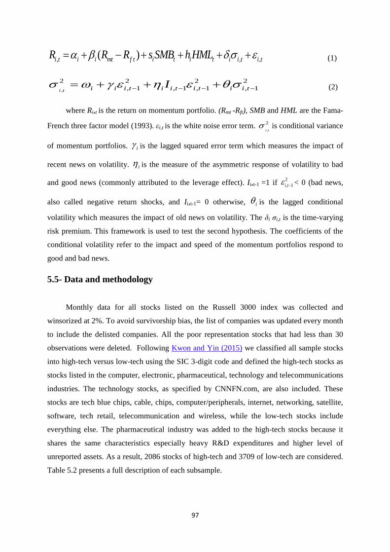
97

, , ,( )i t i i mt f t i t i t i i t i tR R R s SMB h HML (1)

,

2 2 2 2

, 1 , 1 , 1 , 1i t i i i t i i t i t i i tI (2)

where Ri,t is the return on momentum portfolio. (Rmt -Rft), SMB and HML are the Fama-

French three factor model (1993). εi,t is the white noise error term. ,

2

i t is conditional variance

of momentum portfolios. i is the lagged squared error term which measures the impact of

recent news on volatility. i is the measure of the asymmetric response of volatility to bad

and good news (commonly attributed to the leverage effect). Ii,t-1 =1 if 2

, 1i t < 0 (bad news,

also called negative return shocks, and Ii,t-1= 0 otherwise, i is the lagged conditional

volatility which measures the impact of old news on volatility. The δi ζi,t is the time-varying

risk premium. This framework is used to test the second hypothesis. The coefficients of the

conditional volatility refer to the impact and speed of the momentum portfolios respond to

good and bad news.

5.5- Data and methodology

Monthly data for all stocks listed on the Russell 3000 index was collected and

winsorized at 2%. To avoid survivorship bias, the list of companies was updated every month

to include the delisted companies. All the poor representation stocks that had less than 30

observations were deleted. Following Kwon and Yin (2015) we classified all sample stocks

into high-tech versus low-tech using the SIC 3-digit code and defined the high-tech stocks as

stocks listed in the computer, electronic, pharmaceutical, technology and telecommunications

industries. The technology stocks, as specified by CNNFN.com, are also included. These

stocks are tech blue chips, cable, chips, computer/peripherals, internet, networking, satellite,

software, tech retail, telecommunication and wireless, while the low-tech stocks include

everything else. The pharmaceutical industry was added to the high-tech stocks because it

shares the same characteristics especially heavy R&D expenditures and higher level of

unreported assets. As a result, 2086 stocks of high-tech and 3709 of low-tech are considered.

Table 5.2 presents a full description of each subsample.

98

The methodology of Jagadeesh & Titman (1993) was followed to construct equally

weighted portfolios using two breakpoints 10% and 30%. This means that the securities in the

bottom 10 (30) percent are positioned in the loser portfolio, while the securities in the top 10

(30) percent are positioned in the winner portfolio. For the robustness checks, the 30%

breakpoint was chosen following Chui, Titman, & Wei (2003). The main reason why we

implement robustness check is to ensure regression estimates are insensitive to different

market conditions and are insensitive to different assumptions. At the end of each month all

stocks in the high-tech and low-tech samples were ranked in ascending order based on their

past J-months cumulative returns with dividends (J= 3, 6, 12 months). Each of these

portfolios is held for K-months (K=3, 6, 12 months). The momentum portfolio was measured

as a J-K portfolio. This gaves a total of 18 portfolios (nine for the high-tech stocks and nine

for the low-tech stocks). We skipped one -month between the portfolio formation period and

the holding period to relieve the effect of nonsynchronous trading and bid-ask spread, leading

to greater strength in our test. We constructed an overlapping portfolio that consisted of the

winner (loser) portfolios in the previous K months. The returns on the winner/loser portfolios

were the simple average of the returns on the K winner (loser) portfolios. For example, if we

had been going to form a portfolio with 6-months holding period, we would have computed

the simple average of the returns on the six winner (loser) portfolios. In other words, it is

August return on the winner (loser) portfolio is the simple average of the August returns on

the winner (loser) portfolios that constructed from January to June and July that was skipped.

The momentum portfolio („zero-cost‟) in this context equals winners-minus-losers portfolio.

All momentum portfolios were regressed on the three-factor model of Fama-French (1993),

which is described as model 1. Table 5.1 provides detailed descriptions of all the dependent

and independent factors.



5.6.1- Summary statistics

Table 5.2 provides the contribution of each industry in the high-tech stocks and low-

tech stocks determined by the SIC three digits for high-tech stocks and the Fama-French

industrial classification for low-tech stocks. The computer and data processing industry is the

99

largest industry among the high-tech stocks, which represents 21.43%. The second largest

industry is the pharmaceutical and represents 15%. They together make up one-third of the

high-tech stocks. In the other category, construction materials and banks dominate 41.5% of

the low-tech stocks.


Table 5.7 compares the descriptive statistics between the high-tech and low-tech stocks

for each 6-6 momentum portfolio including price, institutional ownership, Beta, EPS,

leverage, turnover and size. We did not notice any difference between the high-tech stocks

and the low-tech stocks. For both subsamples, there is a U-shaped relationship between

momentum returns and both of Beta and Turnover. However, the relationship between

momentum returns and each of Price, Institutional Ownership, EPS, Leverage and Size

formed an inverted U-shape. This means that the loser portfolio has lower Price, Institutional

Ownership, EPS, Leverage and Size but has higher Beta and Turnover than the winner

portfolio in both samples. Nevertheless, on average the high-tech portfolios had lower Price,

lower Institutional Ownership, much lower EPS, much lower Leverage, and lower Size than

the low-tech stocks but they had higher Beta and Turnover than the low-tech stocks. The t-

statistics in Panel B shows significant differences between the high-tech and low-tech for all

variables and portfolios.


The noticeably high Leverage measured by debt to equity can be attributed to the

finance sector since both categories have some financial companies; the miscellaneous

investing in high-tech subsample represents 13% of the sample and the finance sector,

including banks, insurance, financial trading and real estate represent about 25% of the low-

tech R&D sample.

100

5.6.2- Momentum

Table 5.8 and 5.9 compare the summary statistics between the high-tech stocks and

low-tech stocks including mean returns, standard deviation and reward-to-risk for each

momentum portfolios. The rows represent the ranking periods (J=3, 6 and 12 months) and the

columns represent the holding periods (K=3, 6 and 12 months). Our robust findings for the

high-tech stocks, using the breakpoints 10% and 30%, challenge the rational expectation

theory, since the portfolios with higher risk do not provide higher returns. For example, the 6-

6 strategy provides the highest risk-adjusted returns 0.205 and 0.169 for the breakpoints 10%

and 30% respectively, while they do not embody the highest risk. Moreover, the 3-3 strategy

is the lowest volatile strategy, but it does not provide the lowest risk-adjusted returns using

the 10% and 30% breakpoints. For low-tech stocks, the finding provides strong support for

inconsistency with the rational expectation theory. For example, the 12-12 strategy using the

breakpoints 10% and 30%, is the highest volatile strategy, but it does provide the lowest risk-

adjusted returns for the two breakpoints.



Panel D in Tables 5.8 and 5.9 provides t-statistics that are needed to test our first

hypothesis. To facilitate the exposition, we can say that four strategies show larger significant

momentum profits in high-tech stocks than low-tech stocks do, namely, the 3-3 strategy, the

3-6 strategy, the 6-3 strategy and the 6-6 strategy, since the t-statistics show significant

difference between them at 5% significance level. This finding is robust to different

breakpoints. Another important support for the first hypothesis comes from the fact that the

low-tech momentum portfolios never outperform the high-tech ones. In sum, we accept the

first hypothesis for the above mentioned strategies and reject it otherwise. This finding

appears consistent with that of (Wang, 1993) who develops a model of asset pricing under

information asymmetry. In his model, the economy has two kinds of investors, informed and

uninformed investors. He assumes that all investors know current dividends and stock prices,

but informed investors („insiders in our case‟) have certain expectations of the growth rate of

101

future dividends and uninformed ones („outsiders in our case‟) do not. It is known that the

increase in stock prices depends on the growth rate of dividends. As a result, any change in

stock prices can be attributed to the growth rate of dividends. If we assume that the

uninformed investors build rational expectation about the state of the economy using prices

and dividends, then the stocks prices should be considered as true and fundamental values

because the market has frictions and is incomplete. Under the incomplete market

assumptions, investors face different information which leads them to reach different return

expectations. Therefore, the less informed investors, the outsiders in our case who do not

have sufficient information on future dividends and prices, base their trading on realized

returns only to know about the state of the economy, which increases the reliance of their

expected returns on past returns and creates higher momentum for high-tech stocks compared

to low-tech stocks. Therefore, it seems plausible for investors to follow the opposite of

momentum strategy by adopting a long position in the loser portfolio and a short position in

the winner portfolio for low-tech stocks

5.6.3 Asymmetric volatility

Consistently with the GARCH family models, the coefficients of the variance equation

should be positive, except for the asymmetric coefficient in the GJR framework. We check

this condition for all portfolios and it satisfied all of them except the 3-6 strategy in the high-

tech stocks, which has a negative intercept. Fortunately, however, it is insignificant.

Table 5.10 and 5.11 report estimates of Fama-French models (1) and (2) that include a

GJR-GARCH-M term. To facilitate the exposition, the average estimates across the ranking

and holding periods of the coefficients are discussed. The coefficients of and In system

(1) and (2) associate with the lagged square error term and, calibrate the effect of recent news

on the volatility of momentum returns. For the high-tech stocks, using the 10% and 30%

breakpoints the average + /2 of the Fama-French model equals 0.597 and 0.643

respectively, and 0.312 and 0.338 for low-tech stocks respectively. From this discussion, we

found robust and valuable conclusions. The first is that the impact of recent news on the

volatility of high-tech stocks is greater than this impact for low-tech stocks. This is consistent

with the information asymmetry view since the flow of information in the case of higher

levels of information asymmetry creates higher levels of dispersion of belief and leads to a

higher level of volatility (Shalen, 1993).

102



The coefficient in systems (1) and (2) reflects the effect of old news („lagged

conditional variance‟) on the volatility of momentum returns. For high-tech stocks, the

average coefficients are 0.430 and 0.378 using 10% and 30% respectively. For low-tech

stock, the average coefficients are 0.554 and 0.416 using 10% and 30% respectively.

The above discussion reaches the robust conclusion that the impact of old news on volatility

for the high-tech stocks is smaller than that impact for the low-tech stocks. This result is

robust to different breakpoints.

In testing our second hypotheses, the empirical evidence provides a reasonably robust

support. For high-tech stocks, the asymmetric coefficients are insignificant at 5% level for the

whole nine momentum portfolios using the 10% breakpoint, while 7 out of 9 momentum

portfolios show insignificant asymmetric coefficients 𝜂 using 30% breakpoint at 5%

significance level. The insignificant coefficients indicate that the variance responds

symmetrically to good and bad news, indicating high-tech stocks, which are characterized by

higher information asymmetry, leading the investor to lack the required information to herd

and to interact with contrarian investors to induce asymmetric volatility. This symmetric

volatility is robust to different momentum strategies and to different breakpoints. However,

for the low-tech stocks, the asymmetric coefficient 𝜂 in 7 out of 9 momentum portfolios is

significant and 6 out of 9 momentum portfolios have significant asymmetric coefficients

𝜂 at the 5% significance level using 10% and 30% breakpoints respectively. The

significant coefficient means that the impact of bad news (‘ g t v tu s cks’) on

volatility is greater than the impact of good news (‘ s t v tu s cks’), indicating

that the non-intensive firms disclose more information, which helps the irrational

investors to herd and to interact with contrarian investors to induce asymmetric

volatility.

Finally, the last row in each panel in Tables 5.10 and 5.11 presents the persistence

in volatility proxied by 𝛾+ 𝜂/2+ . The above tables present robust evidence that the

103

volatility of high-tech stocks is more persistent than that of low-tech stocks. For the high-tech

stocks, the average 𝛾+ 𝜂/2+ is 1.026 and 1.013, respectively, using 10% and 30%

breakpoints. For the low-tech stocks, however, it is 0.886 and 0.754 respectively. In theory,

volatility persistence means that shocks of current conditional variance have a significant

impact on the variance of the next periods and this persistence is attributed to the persistence

in the information flow proxied by trading volume. The explanation here is that when new

information reaches the stock market, investors react by trading until stock prices attain a

equilibrium point. Investors, then, form new expectations concerning the new equilibrium

point (Andersen, 1996). Therefore, the more persistent volatility for the high-tech stocks is

due to the higher ratio of turnover based on trading volume as shown in Table 5.7 as a proxy

for information flow since the turnover for the high-tech stocks is 0.009 compared with 0.007

for low-tech stocks. Table 5.7 shows that high-tech stocks experience higher levels of

systematic risk measured by beta and smaller size. This conclusion is consistent with

Koutmos, Lee, & Theodossiou (1994) who confirm that volatility persistence is stronger

among stocks with higher systematic risk and among stocks with smaller size.

5.6.4- Idiosyncratic risk -momentum return relation

Tables 5.10 and 5.11 also present the impact of conditional volatility on return through

coefficients that measure the idiosyncratic risk -momentum return relationship. For the

high-tech stocks, 8 out of 9 momentum strategies show an insignificant relation between

idiosyncratic risk and momentum returns at 5% significance level using the 10% breakpoint

and 8 out of 9 coefficients are insignificant using the 30% breakpoint, which obviously

indicates that there is no idiosyncratic risk -momentum return relation at 5% significance

level. These results mean that idiosyncratic risk does not limit arbitrage among momentum

stocks, while momentum is induced as a consequence of mispricing that continues due to

limited arbitrage; and that the transaction cost is high enough to prevent the arbitrageurs from

correcting the momentum effect.

At the same time, for the low-tech stocks 6 out of 9 show a significant and negative

idiosyncratic risk -momentum return relation using the 10% breakpoint and 9 out of 9 are

significant and negative using the 30% breakpoint at 5% significance level. This finding

strongly supports our third hypothesis that the idiosyncratic risk -momentum return for the

high-tech stocks is weaker than that for the low-tech stocks and upholds the role of high

104

transaction cost rather than idiosyncratic risk in limiting arbitrage (Lesmond, Schill, & Zhou,

2004).

Since the negative relation between idiosynctratic risk and momentum return denies the

standard finance theory, Another robustness check is ran using GARCH-M model to provide

additional support for this negative relation using the same breakpoints 10% and 30%. The

finding of GARCH-M supports the previous finding of GJR-GARCH-M which indicates the

first conclusion is robust to the simplified GARCH-M model in Tables 5.12 and 5.13. For the

high-tech stocks using GARCH-M, all nine coefficients are insignificant using 10% and

30% breakpoints at 5% significance level. However, 8 out 9 of the coefficients of the low-

tech stocks are significant and negative using the 10% and 30% breakpoints at 10%

significance level. Tables 5.8 and 5.9 show that most low-tech stocks generate losses and the

corresponding t-statistics are significant for the longest holding period. This finding is

consistent with De Bondt & Thaler (1985) who document the reversal pattern on the long -

term. This finding suggests that the transaction cost for low-tech stocks is too small to limit

arbitrage, due to lower information asymmetry. Therefore, the idiosyncratic risk is the key

player in limiting arbitrage and inducing reversal in returns.

In contrast to the traditional asset pricing theory and risk-return trade-off, the negative

relation between time-varying idiosyncratic risk and momentum returns means investors do

not require greater risk premium for bearing higher risk and also means momentum returns

are greater among stocks with low idiosyncratic volatility. Instead, in the absence of R&D,

investors who bear higher idiosyncratic risk are penalized with lower momentum returns.

This is consistent with Glosten, Jagannathan, & Runkle (1993) who confirm that this negative

sign is possible in special circumstances such as in times of peak interest rate on savings and

scarce investment opportunities are available. From a behavioural perspective, this negative

relation between predicted volatility and the corresponding risk premium is consistent with

Black & McMillan (2006) and Nam, Pyun, & Kim (2003) who attribute this to investors‟

overreaction to certain market news, especially the negative ones („bad news‟). This news

increases predicted volatility which results in higher required rate of return and lower current

stock prices. The explanation here is, some investors, who believe in mean reversion, become

more optimistic about the future after negative return shocks, accepting lower risk premium.

While McLean (2010) confirms that transaction costs limit arbitrage for the smaller

mispricing and idiosyncratic risk limits the arbitrage among the reversal stocks for the greater

105

mispricing, we find that the high-tech stocks that experience higher transcation costs due to

higher information asymmetry, transaction costs limit the arbitrage among momentum stocks,

while for the low-tech stocks that experience lower transaction cost due to lower information

asymmetry, idiosyncratic risk limits the arbitrage among reversal stocks.

5.6.5- The Performance of Fama-French model

Li, Miffre, Brooks, & O‟Sullivan (2008) contributed to the literature through

demonstrating that momentum profits can be explained by a GJR-GARCH-M without

following Lesmond et al. (2004)‟s methodology based on transaction costs since all

coefficients were insignificant in the framework of GJR-GARCH-M. In our result, Tables

5.10 and 5.12 show the following:

For the high-tech stocks, the Fama-French with GJR-GARCH-M terms can moderately

describe the momentum returns since Table 5.10 shows that 5 out of 9 momentum portfolios

have insignificant coefficients using the 10% breakpoint and Table 5.11 shows that 6 out

of 9 have insignificant coefficients using the 30% breakpoint at 5% significance level.

Using Fama-French with GARCH-M in Tables 5.12 and 5.13 provides robust support for the

previous finding, since Table 5.12 shows that 8 out of 9 coefficients are insignificant using

the 10% breakpoint and all 9 coefficients are insignificant using the 30% breakpoint at 5%

significance level.

For the low-tech stocks, the Fama-French with GJR-GARCH-M terms acts very poorly in

describing momentum returns. Table 5.10 shows that only 2 out 9 coefficient are

insignificant using the 10% breakpoint and 1 out 9 coefficients is insignicant using the

30% breakpoint in Table 5.11 at 5% significance level. Using Fama-French with GARCH-M

term provides a robust support, since only 2 out 9 coefficients are insignificant using the

10% breakpoint at 10% significance level in Table 5.12 likewise in Table 5.13 with the 30%

breakpoint at 10% significance level.



106

From the analysis above, we can conclude that there is robust evidence that Fama-

French with its conditional variance term can apparently better explain momentum returns for

high-tech stocks. Though there is no relation between idiosyncratic risk and momentum, the

model performs better at explaining momentum returns. This confirms the third hypothesis

and means that something else („transaction cost‟) other than idiosyncratic risk limits the

arbitrage and induce momentum.

5.7- Conclusion

This research focused on investigating the systematic disagreements in momentum,

asymmetric volatility and the idiosyncratic risk-momentum return relation between high-tech

stocks and low-tech stocks. The SIC code was used to split the whole dataset into two

samples based on the intensity of R&D expenditures; and the Fama-French with GJR-

GARCH-M term was also used to test our hypotheses. We find that; (1) the high-tech stocks,

relative to low-tech stocks, show greater momentum profits in all portfolios that have a

ranking or holding period of less than 12 months and an insignificant difference between the

two samples otherwise; (2) the high-tech stock show symmetric response to good and bad

news while the low-tech stocks show asymmetric response to good and bad news; (3) for the

high-tech stocks there was no idiosyncratic risk- momentum return relation, while this

relation was significant and negative for the low-tech stocks. Our results are robust to

different breakpoints; (4) there is robust evidence that the ability of Fama-French with

conditional variance term to explain momentum returns is better for high-tech stocks than to

low-tech stocks.

These conclusions have many implications: (1) the investor should increase the

proportion of high-tech stocks when constructing the momentum portfolios at the expense of

low-tech stocks to generate greater momentum profits; (2) for the high-tech stocks, the

asymmetric coefficients are econmically and statistcally insignificant, which means that the

variance responds similarly to the positive and negative shocks (good and bad news), while

for the low-tech stocks, the asymmetric coefficients are economically and statistcally

significant, which means that the variance responds to a greater degree in negative returns

shock (bad news) than in positive returns shocks (good news); (3) the finding on idiosyncratic

risk-momentum return relation indicates that, in the case of high-tech stocks, the momentum

returns are compensation for market friction and transcation costs are the key player in

limiting the arbitrage and persisting momentum, while with low-tech stocks that experience

107

lower transaction costs due to lower information asymmetry, idiosyncratic risk limits the

arbitrage and persists reversal in returns. We believe that the next steps in this research

should be to check the robustness of our findings either to data from the emerging markets or

to higher frequency data, such as daily and weekly data or to the other aymmetric conditional

variance models, such as EGARCH model.

108

Tables of results

Table 5.1. Description of the independent variables

Variable Definition

Ri,t Is the return on momentum portfolio.

Winner Includes the stocks in the top 10% (30%) based on past

J-months cumulative returns with dividends.

Loser Includes the stocks in the bottom 10% (30%) based on

past J-months cumulative returns with dividends.

Momentum Is a zero-cost portfolio and measured by winners‟

minus losers‟ portfolio.

( )mt f tR R The excess market returns.

SMB (small minus big) The returns to small firms less the returns to large

firms. We measure a firm‟s size by the market value

of equity at the end of the fiscal year.

HML (high minus low) The returns to high book-to-market firms less The

returns to low book-to-market firms. We measure the

book to market ratio as the fiscal year-end book value

of common equity over the calendar year-end market

equity (December).

,i t White noise error term.

,

2

i t Conditional variance of the momentum portfolios.

i Lagged squared error term measuring the impact of

recent news on volatility.

i Measure of the asymmetric response of volatility to

bad and good news (commonly attributed to the

leverage effect).

i Lagged conditional volatility measureing the impact of

old news on volatility.

t Time-varying risk premium.

109

Table 5.2. Summarizes the proportion of each industry in the high-tech stocks versus low-tech stocks

High-tech stocks

Low-tech stocks

3-Digits SIC

code

Industry Number of

firms per

industry

Percentage

(%)

4-Digits SIC code Industry Number of firms

per industry

Percentage

(%)

272 Periodicals 8 0.38 0100-0799 Agriculture 16 0.40

283 Drugs 318 15.20 1000-1119

1400-1499

Mining 33 0.90

355 Special industry

Machinery

26 1.20 1200-1299 Coal 17 0.40

357 Computer and office

equipment

99 4.75 1300-1389 Petroleum and Natural gas 204 5.50

361 Electronic distribution

Equipment

2 0.09 1500-1799 Construction 63 1.70

362 Electronic industrial

apparatus

16 0.70 2000-2099 Food, Soda and Beer 94 2.50

363 Household appliances 8 0.38 2100-2199 Tobacco 9 0.20

364 Electronic lighting and

writing equipment

15 0.72 2200-2399 Textiles 48 1.30

365 Household audio and video

equipment

8 0.38 2400-3996 Construction materials and steel

works

931 25.10

366 Communication equipment 111 5.32 4000-4789 Transportation 145 3.90

367 Electronic components and

accessories

213 10.21 4822-4839 Telegraph, Radio-TV broadcaster

and communication providers

71 1.90

369 Miscellaneous Electronic

components and supplies

28 1.34 4900-4991 Utilities, and power producer 213 5.70

110

Table 5.2. (continued)

High-tech stocks Low-tech stocks

3-Digit

SIC

Code

Industry Number of firms per

industry

Percentage

(%)

4-Digits SIC

code

Industry Number of firms per

industry

Percentage

(%)

381 Search and navigation equipment 19 0.91 5000-5199 Wholesale 147 4.00

382 Measuring and controlling

devices

96 4.60 5200-5999 Retail 326 8.80

386 Photographic equipment and

supplies

8 0.38 6000-6199 Banks 610 16.40

481 Telephone Communication 122 5.85 6200-6299

6700-6799

Financial trading 53 1.40

484 Cable and other pay TV services 33 1.60 6300-6411

Insurance 231 6.20

573 Radio TV and Electronic stores 19 0.91 6500-6611

Real estate 35 0.90

621 Security brokers and dealers 51 2.44 7020-8999 Personal and Business

services

463 12.50

679 Miscellaneous investing 274 13.13

733

Mailing, reception and

stenographic

5 0.24

737 Computer and data processing 447 21.43

738 Miscellaneous business services 112 5.37

873 Research and testing services 47 2.25

Total 2086 99.79 Total 3709 99.7

111

Table 5.3. Unit root test (Augmented Dickey-Fuller) Breakpoint 10%

The regression is used to estimate Augmented Dickey-Fuller statistics. The regression includes up to 12 lags of

the dependent variable with a constant and no trend. It is obvious that all ADF estimates are more negative than

the critical value. This indicates that the null hypothesis H0: series contains a unit root should be rejected. This

means the time series in the table are stationary.


Holding period 3

months

Holding

period 6

months

Holding

period 12

months

Holding

period 3

months

Holding period

6

months

Holding period

12

months

Panel A: Ranking period 3 months

ADF

-4.280 -3.796 -4.822 -5.087 -4.609 -4.008

% Critical value

-3.469 -3.470 -3.472 -3.469 -3.470 -3.472

Panel B: Ranking period 6 months

ADF

-3.525 -3.626 -5.001 -4.079 -3.744 -3.572

% Critical value

-3.470 -3.471 -3.473 -3.470 -3.471 -3.473

Panel C: Ranking period 12 months

ADF

-3.509 -4.556 -4.987 -3.810 -4.031 -3.855

% Critical value

-3.472 -3.473 -3.475 -3.472 -3.473

-3.475

Panel D: Fama-French Factors


(Rm-Rf) SMB HML (Rm-Rf) SMB HML

ADF

-4.030 -4.746 -4.043 -4.030 -5.409 -3.814

% Critical value

-3.467 -3.467 -3.467 -3.467 -3.467 -3.467

112

Table 5.4. Unit root test (Augmented Dickey-Fuller) Breakpoint 30%

The regression is used to estimate Augmented Dickey-Fuller statistics. The regression includes up to 12 lags of

the dependent variable with a constant and no trend. It is obvious that all ADF estimates are more negative than

the critical value. This indicates that the null hypothesis H0: series contains a unit root should be rejected. This

means the time series in the table are stationary.


Holding period 3

months

Holding

period 6

months

Holding

period 12

months

Holding

period 3

months

Holding

period 6

months

Holding period

12

months


ADF

-5.023 -4.120 -4.723 -4.495 -4.298 -3.660

% Critical value

-3.469 -3.470 -3.472 -3.469 -3.470 -3.472


ADF

-3.916 -3.778 -4.757 -4.380 -3.897 -3.531

% Critical value

-3.470 -3.471 -3.473 -3.470 -3.471 -3.473


ADF

-3.777 -4.889 -4.572 -3.833 -3.775 -3.639

% Critical value

-3.472 -3.473 -3.475 -3.472 -3.473 -3.473

Panel D: Fama-French Factors


(Rm-Rf) SMB HML (Rm-Rf) SMB HML

ADF

-4.030 -4.746 -4.043 -4.030 -5.409 -3.814

% Critical

value

-3.467 -3.467 -3.467 -3.467 -3.467 -3.467

113

Table 5.5. ARCH effect „10% Breakpoint‟

Before running a GARCH-family model, it is plausible to check whether ARCH exists in the residuals or not by

employing Engle (1982) test for ARCH effect. The presence of ARCH helps justify a GARCH-family model. P-

values here indicate that all test statistics are significant at 1%, meaning that ARCH exists in all momentum

returns in both subsamples.


Holding period

3

months

Holding

period 6

months

Holding

period 12

months

Holding

period 3

months

Holding

period 6

months

Holding period

12

months


Chi2

45.010 36.948 41.238 59.135 98.489 137.941

P-Value

(0.000) (0.000) (0.000) (0.000) (0.000) (0.000)


Chi2

60.609 118.515 99.505 105.136 123.858 136.470

P-Value

(0.000) (0.000) (0.000) (0.000) (0.000) (0.000)


Chi2

61.273 109.938 99.099 87.141 118.337 106.318

P-Value

(0.000) (0.000) (0.000) (0.000) (0.000) (0.000)

114

Table 5.6. ARCH effect „30% Breakpoint‟

Before running a GARCH-family model, it is plausible to check whether ARCH exists in the residuals or not by

employing Engle (1982) test for ARCH effect. The presence of ARCH helps justify a GARCH-family model. P-

values here indicate that all test statistics are significant at 1%, meaning that ARCH exists in all momentum

returns in both subsamples.


Holding period 3

months

Holding

period 6

months

Holding

period 12

months

Holding

period 3

months

Holding

period 6

months

Holding period

12

months


Chi2

25.927 39.720 71.674 69.522 126.990 174.258

P-Value

(0.000) (0.000) (0.000) (0.000) (0.000) (0.000)


Chi2

68.324 93.349 115.380 118.479 139.339 162.204

P-Value

(0.000) (0.000) (0.000) (0.000) (0.000) (0.000)


Chi2

88.480 127.754 106.696 110.825 133.583 152.618

P-Value

(0.000) (0.000) (0.000) (0.000) (0.000) (0.000)

115

Table 5.7. portfolios characteristics based on 6-6 momentum strategy using 10% breakpoint

High-tech stocks

Low-tech stocks

Portfolios Price INS Beta EPS LEV TUR Size

(billions)

Price

INS Beta EPS LEV TUR Size

(billions)

P1 16.061

50.834 1.390 -0.279 1.491 0.013 1.430 24.034 72.568 1.119 1.140 2.848 0.010 2.670

P2

20.385 58.433 1.292 0.231 1.422 0.010 2.860 28.069 73.021 1.017 1.648 3.075 0.008 4.020

P3

23.016 61.568 1.209 0.516 1.476 0.009 3.750 30.203 72.433 0.980 1.846 3.263 0.007 4.760

P4 24.991

64.044 1.163 0.701 1.606 0.009 4.460 31.716 72.226 0.951 1.957 3.411 0.006 5.190

P5

27.119 65.222 1.118 0.814 1.671 0.008 4.990 32.972 71.892 0.936 2.022 3.487 0.006 5.470

P6

28.529 66.913 1.094 0.877 1.738 0.008 5.400 33.184 72.743 0.935 2.042 3.511 0.006 5.630

P7 29.346

67.186 1.085 0.930 1.730 0.008 5.600 33.556 72.988 0.933 2.029 3.485 0.006 5.550

P8

30.052 66.712 1.098 0.875 1.710 0.008 5.390 34.176 73.768 0.956 2.001 3.365 0.007 5.550

P9

29.880 65.382 1.179 0.700 1.656 0.009 4.920 33.854 75.019 0.985 1.887 3.214 0.007 5.090

P10

28.818 61.632 1.329 0.270 1.558 0.012 3.350 33.572 76.578 1.085 1.557 2.924 0.009 4.010

Average

25.820 62.793 1.196 0.563 1.606 0.009 4.215 31.534 73.324 0.990 1.813 3.258 0.007 4.794

This table shows several characteristics of ten momentum portfolios that are formed following Jagadeesh and

Titman (1993) and based on six-month returns and held for six months. P1 through P10 represent momentum

portfolios, with P1 containing past losers and P10 containing past winners. Price is the average monthly closing

prices. INS denotes institutional ownership and proxied by the average percentage ratio of free traded shares held

by institutions to the number of float shares outstanding. BETA is the average systematic risk and was calculated by

the CAPM for the past two years of weekly data using the S&P 500 in addition. EPS is computed as net income

available to common shareholders divided by the basic weighted average shares outstanding and the most recent 12

months (trailing 12 months) are summed. LEV denotes leverage and is the average ratio of debt to equity. TUR

denotes turnover and is the average ratio of a shares monthly trading volume divided by the monthly shares

outstanding. Size is the average monthly market capitalization.

116


Panel B: t-statistics for each portfolio and each factor

(*) Significant at 10%, otherwise all is either significant at 5% or insignificant in two tailed tests.

Portfolio Price Institutional Beta EPS Turnover Leverage Size

(in billions)

P1 -37.044

-49.771 30.153 -78.443 24.540 -42.717 -23.473

P2

-34.989 -33.966 34.686 -80.949 28.890 -53.057 -14.974

P3

-31.721 -25.701 30.849 -76.881 29.306 -57.141 -11.303

P4 -28.955

-19.600 29.847 -72.639 26.615 -56.044 -7.506

P5

-24.268 -16.045 26.565 -68.520 25.964 -55.803 -4.688

P6

-19.159 -14.100 23.466 -66.485 23.619 -53.713 -2.205

P7 -17.274

-14.019 22.561 -63.464 21.088 -53.507 0.481

P8

-16.528 -16.886 20.767 -63.750 21.356 -51.048 -1.57

P9

-15.766 -22.646 26.842 -66.995 21.824 -48.191 -1.705*

P10

-18.183 -34.141 29.627 -69.285 25.857 -42.149 -8.846

117

Table 5.8. Summary statistics of momentum portfolios based on 10% breakpoint

Momentum is a portfolio that buys the winner portfolio (top 10% of stocks) and sells the loser portfolio (bottom

10% of stocks) short. Returns are measured as proportions rather than percentages. Reward-to-risk ratio is the

ratio of monthly mean to the monthly standard deviation. The t-statistics in parentheses are for the significance of

the mean. (*) indicates 10% significant level and we use 5% otherwise.


Holding period 3

months

Holding

period 6

months

Holding period

12

months

Holding

period 3

months

Holding period

6

months

Holding

period 12

months


Mean 0.009

(1.67)*

0.017

(1.44)

-0.007

(-2.31)

-0.007

(-0.67)

-0.007

(-1.20)

-0.015

(-2.05)

St. Deviation

0.081 0.123 0.178 0.063 0.097 0.122

Reward-to-risk 0.111 0.138 -0.039 -0.111

-0.072 -0.123


Mean

0.017

(2.53)

0.026

(2.85)

-0.018

(-1.37)

-0.005

(-1.35)

-0.007

(-1.05)

-0.023

(-2.59)

St. Deviation

0.097 0.127 0.197 0.066 0.108 0.136

Reward-to-risk 0.175 0.205 -0.091 -0.076 -0.065

-0.169


Mean 0.010

(1.37)

-0.001

(-0.10)

-0.055

(-3.69)

-0.006

(-1.30)

-0.016

(-2.20)

-0.047

(-4.23)

St. Deviation

0.105 0.150 0.219 0.076 0.115

0.167

Reward-to-risk 0.095 -0.007 -0.251 -0.079 -0.139

-0.281

Panel D: t-statistics between the two groups

Holding Period 3 months Holding Period 6 months Holding Period 12 months

Ranking Period

3 months

2.159 2.553 0.637

Ranking Period

6 months

2.840 2.863 0.389

Ranking Period

12 months

1.876 1.301 -0.385

118

Table 5.9. Summary statistics of momentum portfolios: Robustness analysis based on 30% breakpoint

Momentum is a portfolio that buys the winner portfolio (top 30% of stocks) and sells the loser portfolio (bottom

30% of stocks) short. Returns are measured as proportions rather than percentages. Reward-to-risk ratio is the

ratio of monthly mean to the monthly standard deviation. The t statistics in parentheses are for the significance of

the mean. We use 5% significance level.


Holding period 3

months

Holding

period 6

months

Holding period

12

months

Holding

period 3

months

Holding period

6

months

Holding

period 12

months


Mean 0.001

(0.35)

0.005

(1.27)

-0.003

(-0.50)

-0.007

(-3.46)

-0.008

(-2.86)

-0.014

(-3.26)

St. Deviation

0.049 0.067 0.107 0.030 0.046 0.063

Reward-to-risk 0.020 0.075

-0.028 -0.233 -0.174 -0.222


Mean

0.007

(1.89)*

0.012

(2.37)

-0.006

(-0.96)

-0.005

(-2.33)

-0.005

(-1.56)

-0.014

(-3.00)

St. Deviation

0.056 0.071 0.112 0.031 0.052 0.071

Reward-to-risk 0.125 0.169 -0.053

-0.129 -0.096 -0.197


Mean 0.004

(0.98)

-0.000

(-0.07)

-0.031

(-3.87)

-0.001

(-0.87)

-0.005

(-1.58)

-0.019

(-3.57)

St. Deviation

0.059 0.081 0.120 0.032 0.054

0.079

Reward-to-risk 0.068 0.000 -0.258 -0.031

-0.092 -0.240

Panel D: t-statistics between the two groups

Holding Period 3 months Holding Period 6 months Holding Period 12 months

Ranking Period

3 months

2.107 2.712 1.257

Ranking Period

6 months

2.848 2.829 0.787

Ranking Period

12 months

1.293 0.880 -1.262

119

Table 5.10. Fama-French with a GJR-GARCH-M based on 10% breakpoint


Holding period 3

months

Holding

period 6

months

Holding period

12

months

Holding

period 3

months

Holding period

6

months

Holding period

12

months


α

0.000

(0.01)

0.007

(1.42)

-0.004

(-0.53)

0.011

(2.08)

0.045

(5.34)

0.011

(1.49)

𝛽

-0.092

(-1.07)

0.150

(1.49)

0.200

(1.65)

-0.021

(-0.28)

-0.399

(-4.35)

-0.064

(-0.57)

s

-0.108

(-0.74)

-0.094

(-0.78)

-0.084

(-0.41)

-0.020

(-0.15)

-0.098

(-0.68)

0.017

(0.08)

h

-0.381

(-2.51)

-0.288

(-2.14)

-0.450

(-2.24)

-0.573

(-4.24)

-0.120

(-0.84)

-0.513

(-2.42)

δ

1.738

(1.90)

-0.091

(-0.25)

-0.435

(-1.06)

-4.057

(-1.91)

-6.262

(-3.21)

-1.025

(-1.37)

𝜔

0.000

(1.15)

-0.000

(-0.55)

0.000

(0.41)

0.000

(2.15)

0.001

(3.19)

0.001

(2.26)

𝛾

0.288

(2.32)

0.332

(3.55)

0.481

(2.50)

0.457

(3.19)

0.676

(4.37)

0.698

(2.88)

𝜂

0.192

(1.17)

0.190

(1.23)

-0.236

(-1.34)

-0.305

(-2.19)

-0.627

(-4.10)

-0.446

(-1.93)

0.609

(7.29)

0.609

(13.12)

0.697

(9.30)

0.606

(8.40)

0.533

(8.37)

0.420

(4.74)

𝛾+ 𝜂/2+

0.993 1.036 1.060 0.912 0.896 0.895


α

0.015

(3.07)

0.017

(2.76)

-0.003

(-0.39)

0.010

(1.85)

0.135

(6.25)

0.030

(5.27)

𝛽

-0.138

(-1.61)

0.028

(0.28)

-0.202

(-1.30)

-0.084

(-1.08)

-0.274

(-3.68)

-0.190

(-1.80)

s

-0.097

(-0.80)

0.265

(1.67)

-0.687

(-2.73)

-0.186

(-1.71)

-0.174

(-1.26)

0.246

(1.43)

h

-0.549

(-3.76)

-0.151

(-1.03)

-0.069

(-0.32)

-0.731

(-5.07)

-0.550

(-7.78)

-0.664

(-4.36)

δ

0.379

(0.51)

0.082

(0.17)

-0.582

(-2.20)

-2.538

(-1.26)

-31.798

(-5.19)

-1.230

(-3.22)

𝜔

0.000

(1.77)

0.001

(2.52)

0.001

(1.68)

0.001

(2.74)

0.001

(3.75)

0.002

(3.09)

𝛾

0.387

(3.25)

0.591

(3.47)

0.819

(3.21)

0.616

(3.12)

0.249

(4.54)

0.922

(3.56)

𝜂

0.396

(1.54)

0.183

(0.72)

-0.346

(-1.31)

-0.122

(-0.51)

-0.342

(-4.91)

-0.601

(-2.29)

0.430

(5.59)

0.294

(3.45)

0.423

(6.03)

0.240

(2.02)

0.777

(19.76)

0.205

(2.83)

𝛾+ 𝜂/2+ 1.015 0.977 1.069 0.795 0.855 0.827

120


This table reports the coefficient estimates for systems (1) and (2) for the momentum portfolios. Momentum is a

portfolio that buys the winner portfolio (top 10% of stocks) and sells the loser portfolio (bottom 10% of stocks)

short. α measures a portfolio‟s abnormal performance, 𝛽 measures the market risk of the portfolio, s and h are the

portfolio loadings based on size and book-to-market factors as measured by Fama and French (1993), δ is the

time-varying risk exposure. The conditional variance of the portfolio returns follows a GJR-GARCH structure as

,

2 2 2 2

, 1 , 1 , 1 , 1i t i i i t i i t i t i i tI where 𝜔, 𝛾, 𝜂 and are estimated parameters

and It-1 takes a value of 1, when εt-1 is negative and a value of 0, otherwise. We use 5% significance level. The t-

statistics are in parentheses.


Holding period 3

months

Holding period 6

months

Holding period 12

months

Holding period 3

months

Holding period 6

months

Holding period 12

months


α

0.002

(0.37)

0.014

(2.52)

-0.024

(-2.35)

0.025

(4.15)

0.098

(4.91)

0.185

(5.70)

𝛽

-0.074

(-0.87)

-0.030

(-0.29)

-0.179

(-1.01)

-0.044

(-0.61)

0.014

(0.19)

-0.268

(-2.99)

s

-0.141

(-0.87)

0.021

(0.17)

-0.628

(-2.61)

-0.221

(-1.79)

0.215

(1.28)

-0.603

(-3.74)

h

-0.793

(-5.02)

-0.096

(-0.86)

-0.069

(-0.29)

-0.710

(-4.99)

0.017

(0.16)

-0.566

(-2.98)

δ

0.480

(0.56)

-0.621

(-1.76)

-0.452

(-1.47)

-7.075

(-2.53)

-17.336

(-4.11)

-19.890

(-4.71)

𝜔

0.000

(1.64)

0.001

(2.26)

0.005

(3.38)

0.000

(2.59)

0.001

(5.30)

0.001

(2.80)

𝛾

0.191

(2.67)

1.334

(3.00)

0.961

(2.77)

0.479

(3.38)

0.205

(4.35)

0.060

(4.47)

𝜂

0.473

(1.89)

-0.615

(-1.32)

-0.263

(-0.67)

-0.244

(-1.99)

-0.216

(-4.25)

-0.214

(-4.87)

0.574

(5.92)

0.115

(2.13)

0.110

(1.50)

0.497

(4.49)

0.740

(16.86)

0.971

(41.66)

𝛾+ 𝜂/2+ 1.002 1.141 0.939 0.854 0.837 0.924

121

Table 5.11. Fama-French with a GJR-GARCH-M: Robustness analysis based on 30% breakpoint


Holding period 3

months

Holding

period 6

months

Holding period

12

months

Holding

period 3

months

Holding period

6

months

Holding period 12

months


α

0.002

(0.93)

0.001

(0.41)

0.004

(0.82)

0.001

(0.46)

0.022

(5.02)

0.060

(4.40)

𝛽

-0.195

(-4.80)

0.026

(0.36)

0.124

(1.32)

-0.055

(-1.74)

-00.123

(-3.09)

0.066

(1.24)

s

-0.275

(-3.75)

-0.027

(-0.27)

-0.278

(-1.74)

-0.149

(-2.40)

-0.186

(-2.36)

-0.014

(-0.19)

h

-0.200

(-3.28)

-0.089

(-1.30)

-0.210

(-1.80)

-0.309

(-5.15)

-0.183

(-2.83)

-0.162

(-2.16)

δ

0.506

(0.33)

0.173

(0.17)

-0.786

(-1.37)

-8.330

(-1.99)

-20.002

(-4.10)

-42.575

(-3.89)

𝜔

0.000

(1.50)

0.000

(2.36)

0.000

(2.01)

0.000

(2.25)

0.000

(2.33)

0.000

(4.19)

𝛾

0.181

(2.36)

0.499

(3.12)

0.779

(2.99)

0.257

(3.01)

0.338

(3.95)

0.265

(3.66)

𝜂

0.334

(3.22)

-0.013

(-0.08)

-0.292

(-1.13)

-0.072

(-0.75)

-0.360

(-3.82)

-0.386

(-3.69)

0.689

(10.16)

0.542

(7.33)

0.367

(3.98)

0.737

(13.10)

0.741

(17.69)

0.661

(10.54)

𝛾+ 𝜂/2+

1.037 1.034 1.000 0.958 0.899 0.733


α

0.002

(0.70)

0.011

(2.88)

-0.023

(-5.52)

0.005

(2.51)

0.015

(4.66)

0.015

(4.35)

𝛽

-0.118

(-2.92)

-0.038

(-0.64)

-0.024

(-0.30)

-0.098

(-3.02)

-0.147

(-4.13)

-0.024

(-0.43)

s

-0.194

(-2.88)

0.024

(0.25)

-0.367

(-3.12)

-0.148

(-2.50)

-0.187

(-2.45)

0.050

(0.64)

h

-0.216

(-3.00)

-0.139

(-1.61)

-0.061

(-0.63)

-0.282

(-6.10)

-0.218

(-2.99)

-0.143

(-1.58)

δ

2.291

(1.96)

-0.809

(-0.91)

0.820

(1.53)

-8.913

(-2.35)

-6.468

(-2.60)

-2.698

(-3.86)

𝜔

0.000

(2.11)

0.001

(3.34)

0.000

(1.61)

0.000

(2.85)

0.000

(4.56)

0.001

(4.05)

𝛾

0.328

(3.67)

0.769

(2.89)

0.491

(3.42)

0.662

(3.37)

0.840

(3.20)

0.980

(4.33)

𝜂

0.712

(2.32)

-0.100

(-0.34)

0.630

(1.62)

-0.264

(-1.30)

-0.663

(-2.30)

-0.744

(-3.17)

0.405

(4.95)

0.210

(2.47)

0.272

(3.14)

0.321

(3.00)

0.041

(0.48)

0.065

(0.87)

𝛾+ 𝜂/2+

1.089 0.929 1.078 0.851 0.549 0.673

122




short. α measures the portfolio‟s abnormal performance, 𝛽 measures the market risk of the portfolio, s and h are

the portfolio loadings based on size and book-to-market factors as measured by Fama and French (1993), δ is the

time-varying risk exposure. The conditional variance of the portfolio returns follows a GJR-GARCH structure as

,

2 2 2 2

, 1 , 1 , 1 , 1i t i i i t i i t i t i i tI where 𝜔, 𝛾, 𝜂 and are estimated parameters

and It-1 takes a value of 1, when εt-1 is negative and a value of 0, otherwise. We use 5% significance level. The t-

statistics are in parentheses.


Holding period 3

months

Holding

period 6

months

Holding period

12

months

Holding

period 3

months

Holding period

6

months

Holding period 12

months


α

0.004

(1.50)

0.004

(0.97)

-0.029

(-5.05)

0.024

(4.56)

0.040

(7.55)

0.035

(8.24)

𝛽

-0.143

(-3.06)

-0.024

(-0.36)

-0.047

(-0.49)

-0.221

(-9.07)

-0.130

(-3.48)

0.054

(1.21)

s

-0.118

(-1.49)

-0.037

(-0.41)

-0.215

(-1.58)

-0.223

(-4.30)

-0.331

(-4.91)

0.350

(3.48)

h

-0.330

(-3.82)

-0.155

(-1.85)*

0.068

(0.59)

-0.430

(-9.55)

-0.418

(-6.43)

0.038

(0.38)

δ

-0.115

(-0.09)

-0.910

(-1.17)

-0.004

(-0.01)

-30.224

(-2.82)

-29.832

(-4.78)

-6.943

(-3.65)

𝜔

0.000

(1.52)

0.001

(4.12)

0.000

(1.81)

0.000

(6.61)

0.000

(2.91)

0.000

(2.43)

𝛾

0.451

(3.17)

0.945

(2.50)

0.590

(2.63)

0.426

(3.08)

0.458

(3.62)

0.613

(3.90)

𝜂

0.151

(0.61)

-0.313

(-0.80)

0.251

(0.80)

-0.522

(-3.34)

-0.460

(-3.72)

-0.117

(-1.32)

0.473

(4.84)

0.156

(2.02)

0.293

(3.07)

0.133

(1.73)

0.633

(8.27)

0.409

(6.58)

𝛾+ 𝜂/2+

0.999 0.944 1.008 0.298 0.861 0.964

123

Table 5.12. Fama-French with a GARCH (1,1)-M based on 10% breakpoint


Holding period 3

months

Holding

period 6

months

Holding period

12

months

Holding

period 3

months

Holding period

6

months

Holding period 12

months


α

-0.000

(-0.09)

-0.001

(-0.15)

-0.003

(-0.50)

0.007

(1.80)*

0.039

(3.89)

0.013

(1.35)

𝛽

-0.170

(-1.90)

-0.024

(-0.13)

0.203

(1.34)

0.019

(0.22)

-0.394

(-3.21)

-0.108

(-0.71)

s

-0.207

(-1.56)

-0.077

(-0.43)

-0.029

(-0.12

-0.004

(-0.03)

-0.177

(-1.00)

-0.008

(-0.03)

h

-0.277

(-1.92)

-0.433

(-1.69)

-0.372

(-1.21)

-0.544

(-2.77)

0.029

(0.13)

-0.430

(-1.08)

δ

1.283

(1.26)

0.084

(0.15)

-0.132

(-0.63)

-2.569

(-2.47)

-3.451

(-3.02)

-0.896

(-1.67)*

𝜔

0.000

(1.36)

-0.000

(-0.00)

0.000

(0.78)

0.000

(1.30)

0.001

(2.24)

0.001

(1.77)

𝛾

0.366

(1.84)

0.213

(2.33)

0.333

(4.70)

0.238

(3.62)

0.484

(2.53)

0.390

(3.76)

0.660

(5.22)

0.814

(11.50)

0.700

(13.52)

0.748

(10.43)

0.467

(3.85)

0.561

(4.38)

𝛾+

1.026 1.027 1.033 0.986 0.951 0.951


α

0.016

(2.95)

0.017

(1.93)

-0.008

(-0.81)

0.011

(1.70)*

0.046

(2.15)

0.053

(3.57)

𝛽

-0.097

(-1.01)

0.079

(0.50)

0.112

(-0.62)

-0.082

(-1.00)

-0.082

(-0.45)

-0.134

(-0.96)

s

-0.127

(-1.02)

0.324

(1.59)

-0.823

(-3.26)

-0.190

(-1.25)

-0.174

(-0.96)

0.057

(0.28)

h

-0.491

(-2.54)

-0.089

(-0.30)

-0.037

(-0.09)

-0.739

(-3.91)

-0.168

(-0.63)

-0.508

(-2.19)

δ

-0.394

(-0.72)

0.027

(-0.07)

-0.404

(-1.39)

-3.329

(-1.78)*

-4.765

(-1.86)*

-3.785

(-2.87)

𝜔

0.001

(1.75)

0.001

(2.01)

0.001

(1.59)

0.000

(1.78)

0.001

(2.12)

0.001

(3.22)

𝛾

0.583

(3.77)

0.517

(4.31)

0.527

(4.02)

0.364

(3.97)

0.479

(4.62)

0.478

(5.36)

0.443

(3.79)

0.441

(4.35)

0.520

(5.09)

0.478

(3.30)

0.415

(3.34)

0.475

(8.62)

𝛾+

1.026 0.958 1.047 0.842 0.894 0.953

124






time-varying risk exposure. The conditional variance of the portfolio returns follows a GARCH (1.1) structure as

2 2 2

1 t 1t t where 𝜔, 𝛾 and are estimated parameters and It-1 takes a value of 1, when εt-

1 is negative and a value of 0, otherwise. (*) indicates 10% significant level and we use 5% significance level

otherwise. The t-statistics are in parentheses.


Holding period 3

months

Holding

period 6

months

Holding period

12

months

Holding

period 3

months

Holding period

6

months

Holding period 12

months


α

0.008

(1.20)

0.012

(1.76)

-0.037

(-1.72)

0.022

(3.17)

0.038

(0.95)

0.119

(3.73)

𝛽

-0.079

(-0.60)

-0.015

(-0.11)

-0.097

(-0.54)

-0.008

(-0.10)

-0.068

(-0.73)

-0.113

(-0.73)

s

-0.102

(-0.54)

0.010

(0.06)

-0.614

(-2.26)

-0.192

(-1.29)

0.056

(0.21)

-0.343

(-1.32)

h

-0.815

(-4.15)

-0.166

(-0.96)

-0.386

(-0.97)

-0.678

(-3.51)

-0.477

(-1.71)

-0.222

(-0.92)

δ

-0.425

(-0.69)

-0.157

(-0.67)

-0.110

(-0.35)

-5.467

(-3.40)

-3.322

(-0.60)

-9.865

(-3.20)

𝜔

0.000

(1.95)

0.001

(2.00)

0.005

(3.45)

0.000

(2.44)

0.001

(2.24)

0.001

(3.71)

𝛾

0.331

(3.46)

0.923

(5.47)

0.952

(5.01)

0.398

(4.23)

0.634

(1.52)

0.300

(6.53)

0.642

(7.49)

0.201

(1.87)

0.054

(0.76)

0.491

(5.43)

0.208

(0.56)

0.590

(20.44)

𝛾+

0.973 1.124 1.006 0.889 0.842 0.890

125

Table 5.13. Fama-French with a GARCH (1,1)-M: Robustness analysis based on 30% breakpoint


Holding

period 3

months

Holding

period 6

months

Holding period

12

months

Holding

period 3

months

Holding period

6

months

Holding period 12

months


α

0.004

(1.09)

0.001

(0.31)

-0.004

(-0.51)

0.001

(0.48)

-0.001

(-0.31)

0.010

(2.52)

𝛽

-0.183

(-2.59)

0.027

(0.35)

0.141

(1.59)

-0.051

(-1.15)

-0.095

(-1.56)

0.055

(1.09)

s

-0.231

(-2.50)

-0.027

(-0.27)

-0.283

(-1.88)

-0.146

(-1.84)

-0.255

(-2.53)

-0.106

(-1.11)

h

-0.125

(-1.23)

-0.089

(-0.69)

-0.223

(-1.40)

-0.305

(-3.23)

-0.355

(-2.67)

-0.132

(-1.22)

δ

-1.212

(-0.63)

0.205

(0.33)

-0.107

(-0.20)

-7.579

(-2.92)

3.168

(1.12)

-3.185

(-2.26)

𝜔

0.000

(1.30)

0.000

(1.68)

0.000

(2.42)

0.000

(1.31)

0.000

(1.58)

0.001

(3.22)

𝛾

0.192

(2.14)

0.491

(3.83)

0.489

(4.33)

0.213

(2.86)

0.179

(3.79)

0.824

(3.79)

0.803

(10.56)

0.542

(4.92)

0.509

(5.66)

0.753

(8.00)

0.800

(17.04)

0.124

(0.97)

𝛾+

0.995 1.033 0.998 0.966 0.979 0.948


α

0.004

(1.39)

0.005

(0.97)

-0.009

(-0.80)

0.007

(1.92)*

0.014

(2.23)

0.063

(5.22)

𝛽

-0.116

(-1.98)

-0.084

(-0.90)

-0.064

(-0.59)

-0.084

(-2.07)

-0.163

(-2.26)

-0.018

(-1.04)

s

-0.223

(-2.49)

0.047

(0.51)

-0.480

(-309)

-0.185

(-2.19)

-0.261

(-2.45)

-0.004

(-0.03)

h

-0.171

(-1.32)

-0.081

(-0.64)

-0.004

(-0.03)

-0.258

(-3.10)

-0.234

(-0.87)

-0.225

(-4.09)

δ

-0.211

(-0.18)

0.589

(1.01)

-0.153

(-0.35)

-9.538

(-2.61)

-4.688

(-1.81)*

-25.336

(-3.24)

𝜔

0.000

(1.93)

0.001

(2.15)

0.000

(1.55)

0.000

(1.46)

0.000

(1.28)

0.000

(2.63)

𝛾

0.471

(4.12)

0.637

(4.79)

0.409

(3.80)

0.443

(3.62)

0.448

(2.58)

0.394

(3.18)

0.544

(6.58)

0.316

(2.28)

0.580

(4.75)

0.424

(2.21)

0.545

(3.36)

0.434

(5.77)

𝛾+

1.015 0.953 0.989 0.867 0.993 0.828

126






time-varying risk exposure. The conditional variance of the portfolio returns follows a GARCH (1.1) structure as

2 2 2

1 t 1t t where 𝜔, 𝛾 and are estimated parameters and It-1 takes a value of 1, when εt-

1 is negative and a value of 0, otherwise. (*) indicates 10% significant level and we use 5% significance level

otherwise. The t-statistics are in parentheses.


Holding

period 3

months

Holding

period 6

months

Holding period

12

months

Holding

period 3

months

Holding period

6

months

Holding period 12

months


α

0.005

(1.77)

0.002

(0.32)

-0.025

(-1.12)

0.014

(2.35)

0.011

(3.83)

0.055

(9.10)

𝛽

-0.126

(-2.03)

-0.017

(-0.19)

0.026

(0.25)

-0.085

(-1.33)

-0.036

(-0.67)

-0.030

(-0.89)

s

-0.104

(-1.30)

-0.052

(-0.49)

-0.151

(-0.91)

-0.249

(-2.56)

-0.090

(-0.87)

0.018

(0.24)

h

-0.358

(-3.56)

-0.151

(-1.08)

-0.072

(-0.23)

-0.418

(-3.56)

-0.756

(-6.80)

-0.182

(-2.42)

δ

-0.620

(-0.68)

-0.325

(-0.73)

-0.444

(-0.66)

-14.737

(-1.91)*

-1.750

(-3.21)

-19.259

(-6.88)

𝜔

0.000

(1.75)

0.001

(3.03)

0.001

(2.19)

0.000

(1.29)

0.000

(4.44)

0.000

(2.83)

𝛾

0.391

(4.21)

0.792

(5.35)

0.694

(5.28)

0.417

(2.35)

1.066

(3.84)

0.409

(7.41)

0.624

(10.10)

0.150

(1.27)

0.296

(3.33)

0.352

(1.27)

0.010

(0.32)

0.595

(15.95)

𝛾+

1.015 0.942 0.990 0.769 1.076 1.004

127

Chapter Six

Concluding Remarks

The traditional framework EMH/CAPM has faced plenty of criticisms concerning its

empirical failures that are attributed to its unrealistic assumptions such as assuming that all

agents in financial markets are rational and able to perceive all information and form proper

expectations. In addition, this traditional framework suffers from a failure to explain how

individual investors take their investments decisions and a failure to explain the way that they

follow in forming their portfolios. Behavioural Finance employs the principles of cognitive

psychology to construct a more realistic body of knowledge and is formed of two building

blocks: (1) people are susceptible to systematic cognitive biases and these biases have an

impact on asset prices; (2) involving human beings in financial markets studies helps improve

our understanding of financial phenomena.

This thesis makes a number of concluding remarks and suggests several policy

implications that can be organized as follows:

The main conclusion of Chapter 3 is that irrational investors think “good stocks are the

stocks of good companies”. As a result, they prefer to buy the stocks of good companies that

are characterized by higher earnings per share as profitability, higher financial leverage,

higher growth, larger size and lower CF/P since the lower level of liquidity reflects the

underuse of corporate assets leading to corporate losses. The policy implications come from

the idea in behavioural finance that stipulated irrational („uniformed‟) investors destabilize or

divert prices away from fundamental value. Rational („informed‟) investors stabilize asset

prices and back prices to the fundamental value through exploiting the systematic cognitive

biases of the irrational investors. In this paper, we use the capital gains overhang as a proxy

for the unrealized capital gains encounted by the PT/MA investors to forecast a cross section

of expected returns. Therefore, we expect the momentum in stock returns to be the most

important implication of the PT/MA framework. In this context, our paper has wide

implications because it guides the momentum traders to increase the proportion of stocks of

good companies that are characterized by higher earnings per share, higher financial leverage,

higher growth, larger size and lower turnover in their portfolios, because stocks of this kind

128

are more susceptible to being traded by irrational investors and accordingly generate a higher

capital gains overhang. Finally, further research is required especially in emerging markets to

provide empirical support for the applicability of our findings to emerging markets.

Chapter 4 contains new findings. For instance, the impact of capital gains overhang on

expected returns differs across the expected returns distribution, which indicates that the

relation between capital gains overhang and expected returns is nonlinear. This finding offers

implications for researchers that the OLS conventional technique is less informative and not

appropriate for introducing a full description of the relation between capital gains overhang

and expected returns; instead, a broader and more flexible quantile regression technique

should be used. The second contribution of this chapter is to show how well the disposition

effect works in driving momentum profits at the 0.05th

and 0.95th

expected returns quantiles.

However, there is robust evidence that the disposition effect is not a good noisy proxy for

inducing intermediate momentum at the lowest 0.05th

expected returns quantile. At the

highest 0.95th

expected returns quantile, the disposition effect induces contrarian rather than

momentum returns. The implications are that the disposition effect can be considered the

principal element in discerning return persistence anomalies at the 0.95th

expected return

quantile and the principal element in discerning the price reversal anomaly. However, it

seems that the risk-based explanation plays the major role at the lowest 0.05th

expected

returns quantile. Finally, future works might do to shed light on emerging markets especially

fast growing markets such as the Chinese stock market, to empirically support these

interesting new findings.

Chapter 5 bridges at least three research gaps through examining the systematic

differences in momentum, asymmetric volatility and the idiosyncratic risk-momentum returns

relation between high-tech stocks and low-tech stocks. The first conclusion is that four

momentum strategies explain the significant and robust larger momentum returns in high-

tech stocks than low-tech stocks. These strategies are the 3-3 strategy, the 3-6 strategy, the 6-

3 strategy and the 6-6 strategy. The implication here is that the momentum traders should

increase the fraction of high-tech stocks in their portfolios at the expense of low-tech stocks

to make greater momentum profits. The second conclusion is that there is robust evidence

that the volatility responds symmetrically to good and bad news in high-tech stocks, while it

responds asymmetrically in low-tech stocks. This finding has many implications for investors

129

and policy makers. For instance, in low-tech stocks the risk and cost of equity may surge

more when facing negative market returns shocks than when facing positive market returns

shocks, because of the asymmetric volatility. However, in the high-tech stocks the negative

and positive market returns shocks make the same impact on volatility and in turn they make

the same impact on risk and the cost of capital. Another implication is in the area of option

pricing because the stock market volatility is a key determinant of option prices. For low-tech

stocks, the arrival of good and bad news leads to higher volatility in response to negative

return shocks than to positive return shocks which results in higher option price in the case of

negative return shocks than positive return shocks. For the high-tech stocks, the arrival of

good and bad news should have the same impact on option prices.

The third conclusion is that, there is no robust evidence of idiosyncratic risk-

momentum return relation in the high-tech stocks, while this relation is significantly negative

in the low-tech stocks. This finding is robust to different breakpoints. It is also consistent

with the behaviourally-based explanation and supports the role of high transaction cost in

limiting the arbitrage process rather than idiosyncratic risk, which makes the relation of

idiosyncratic risk and momentum is stronger among low-tech stocks than high-tech stocks.

However, this relation is negative for low-tech stocks. This means that, for the high-tech

stocks which experience the higher transcation costs associated with higher information

asymmetry, the transaction costs limit arbitrage among momentum stocks, while for the low-

tech stocks that experience lower transaction cost due to lower information asymmetry,

idiosyncratic risk limits arbitrage among reversal stocks.

Finally, a replication of this research using emerging markets data is recommended to

ensure that these findings are generalizable to emerging markets. The implication for

researchers here is that this finding improves our understanding of the relative importance of

idiosyncratic risk and transaction costs in the limiting arbitrage mechanism and inducing

momentum. It also serves the theoretical debate on the sources of momentum between the

risk-based school of thought and behaviourally-based school of thought.

This first limitation in this thesis is that it considers two cognitive biases only, namely,

disposition effect and herding behaviour. However, other cognitive biases such as heuristics,

representativeness, framing, overconfidence and conservatism are part of our research agenda

for future works. The data used throughout the thesis focused mainly on the US stock market.

130

Therefore, our findings can be generalized to developed markets. However, the uncertain

applicability of our thesis to emerging markets can be considered as another of its limitations

because the emerging markets are characterized by unique features and require empirical

evidence before our findings can be generalize to.

131

Bibliography Aboody, D., & Lev, B. (2000). Information asymmetry, R&D, and insider gains. The Journal

of Finance 55 (6), 2747-2766.

Aggarwal , R. K., & Jorion, P. (2010). Hidden survivorship in hedge fund returns. Financial

Analysts Journal 66 (2), 69-74.

Alam, P., Liu, M., & Peng, X. (2014). R&D expenditures and implied equity risk premums.

Review of Quantitative Finance and Accounting 43, 441-462.

Alm, l. R., & Mason, S. G. (Eds.). (2007). Linear correlation and regression (2ed

). United

States: Taylor & Francis Group.

Andersen, T. G. (1996). Return volatility and trading volume in financial markets: An

information of stochastic volatility. The Journal of Finance 51 (1), 169-204.

Arena, M. P., Haggard, K. S., & Yan, X. (2008). Price momentum and idiosyncratic

volatility. The Financial Review 43, 159--190.

Asem, E. (2009). Dividends and price momentum. Journal of Banking and Finance 33, 486-

494.

Avramov, D., Chordia, T., & Goyal, A. (2006). The impact of trades on daily volatility. The

Review of Financial Studies 1 (19), 1241-1277.

Bagella, M., Becchetti, L., & Adriani, F. (2005). Observed and 'fundamental' price-earning

ratios: A comparative analysis of high-tech stock evaluation in the US and in Europe.

Journal of International Money and Finance 24, 549-581.

Baillie, R. T., & DeGennaro, R. P. (1990). Stock returns and volatility. The Journal of

Financial and Quantitative Analysis 25 (2), 203-214.

Baker, H. K., & Nofsinger, J. R. (2010). Behavioural finance: An overview. In B. K. H. , & J.

R. Nofsinger, Behavioural Finance: Investors, Corporations and Markets (pp. 3-23).

New Jersey: JohnWiley & Sons, Inc.

Baker, M., & Wurgler, J. (2006). Investor sentiment and the cross-section of stock returns.

Journal of Finance 61 (4), 1645-1680.

Banz, R. W. (1981). The relationship between return and market value of common stocks.

Journal of Financial Economics 9 (1), 3-18.

Barber, B. M., Heath, C., & Odean, T. (2003). Good reasons sell: Reason-based choice

among group and individual investors in the stock market. Management Science 49

(12), 1636-1652.

Barber, B., Odean T., & Zhu, N. (2009). Systematic noise. Journal of Financial Markets 12,

547-569.

132

Barber, B., Odean T., & Zheng, N. (2000). The behavior of mutual fund investors.

Unpublished working paper, University of California.

Barberis, N., & Huang, M. (2001). Mental accounting, loss aversion, and individual stock

returns. The Journal of Finance 56 (4), 1247- 1292.

Barberis, N., Huang, M., & Santos, T. (2001). Prospect theory and asset prices. The Quarterly

Journal of Economics 116, 1-53.

Barberis, N., Shleifer, A., & Vishny, R. (1998). A model of investor sentiment. Journal of

Financial Economics 49, 307-343.

Barberis, N., & Thaler, R. (2003). A survey of behavioural finance. In G. M. Constantinides,

M. Harris, & R. M. Stulz, Handbook of the Economics of Finance (pp. 1052-1119).

Netherlands: Elsevier Science.

Barberis, N., & Xiong, W. (2009). What drives the disposition effect? An analysis of long-

standing preference-based explanation . The Journal of Finance 64, 751-784.

Barone-Adesi, G., Engle, R. F., & Mancini, L. (2008). A GARCH option pricing model with

filtered historical simulation. The Review of Financial Studies 21 (3), 1223- 1258.

Barron, O. E., Byard, D., Kile, C., & Riedl, E. J. (2002). High-technology intangibles and

analysts‟ forecasts. Journal of Accounting Research 40 (2), 289-312.

Barth, M. E., Kasznik, R., & McNichols, M. F. (2001). Analyst coverage and intangible

assets. Journal of Accounting Research 39 (1), 1-34.

Basu, S. (1977). Investment performance of common stocks in relation to their price-earnings

ratios: A test of the efficient market hypothesis. The Journal of Finance 32 (3), 663-

682.

Baur, D. G., Dimpfl, T., & Jung, R. C. (2012 ). Stock return autocorrelations revisited: A

quantile regression approach. Journal of Empirical Finance 19, 254-265.

Baysinger, B., & Hoskisson, R. E. (1990). The composition of boards of directors and

strategic control: Effects on corporate strategy. The Academy of Management Review

15 (1), 72-87.

Ben-David, I, & Hirshleifer, D. (2012). Are investors really reluctant to realize their losses?

Trading responses to past returns and the disposition effect. The Review of Financial

Studies 25 (8), 2485-2532.

Berges, A., McConnell, J. J., & Schlarbaum, G. G. (1984). The turn-of-the-year in Canada.

The Journal of Finance 39 (1), 185-192.

Bhagat, S., & Welch , I. (1995). Corporate research & development investments international

comparisons. Journal of Accounting and Economics 19, 443 470.

133

Bhattacharya, S. (1979). Imperfect information, dividend policy, and 'the bird in the hand'

fallacy. Bell Journal of Economics 10, 259-270.

Bhootra, A., & Hur, J. (2012). On the relationship between concentration of prospect

theory/mental accounting investors, cointegration, and momentum. Journal of

Banking and Finance 36, 1266-1275.

Bilinski, P., & Strong, N. (2013). Managers' private information, investor underreaction and

long-run SEO performance. European Financial Management 19 (5), 956-990.

Birru, J. (2015). Confusion of confusions: A test of the disposition effect and momentum. The

Review of Financial Studies 28 (7), 1849-1873.

Black, F. (1976). Studies in stock volatility changes. American Statistical Association,

Business and Economics statistics section.

Black, A., J., & McMillan, D. G. (2006). Asymmetric risk premium in value and growth

stocks. International Review of Financial Analysis 15, 237-246.

Bolton, P., & Scharfstein, D. S. (1990). A theory of predation based on agency problems in

financial contracting. American Economic Review 80 (1), 93-106.

Bond, S. R., & Cummins, J. G. (2000). The stock market and investment in the new

economy: Some tangible facts and intangible fictions. Brookings Papers on Economic

Activity 1, 61-124.

Brooks, C. (2008). Introductory econometrics for finance (2ed

). New York: Cambridge

University Press.

Brown, S. J., Goetzmann, W., Ibbotson, R. G., & Ross, S. A. (1992). Survivorship bias in

performance studies. The Review of Financial Studies 3 (4), 553-580.

Brunnermeier, M. K., & Nagel, S. (2004). Hedge funds and technology bubble. The Journal

of Finance 59 (5), 2013-2040.

Callahan, C. M., Lee, C. M., & Yohn, T. L. (1997). Accounting information and bid-ask

spreads. Accounting Horizons 11 (4), 50-60.

Callimaci, A., & Landry, S. (2004). Market valuation of research and development spending

under Canadian GAAP. Canadian Accounting Perspectives 3 (1), 33–53.

Cameron, C., & Trivedi, , P. (2010). Microeconometrics using STATA. Texas: STATA press.

Carhart, M. M., Carpenter, J. N., Lynch, A. W., & Musto, D. K. (2002). Mutual fund

survivorship. The Review of Financial Studies 15 (5), 1439-1463.

Chan, K., Karolyi, A., & Stulz, R. M. (1992). Global financial markets and the risk premium

on U.S. equity. Journal of Financial Economics 32, 137-167.

134

Chan, W. S., Frankel, R, & Kothari, S.P. (2004). Testing behavioural finance theories using

trends and consistency in financial performance. Journal of Accounting and

Economics 38, 3–50.

Chan, L. K., Lakonishok, J., & Sougiannis, T. (2001). The stock market valuation of research

and development expenditures. The Journal of Finance 56 (6), 2431-2456.

Chang, X., Dasgupta , S., & Hilary , G. (2006). Analyst coverage and financing decisions.


Chen, G., Kim, K.A., Nofsinger, J.R., & Rui, O.M. (2007). Trading performance, disposition

effect, overconfidence, representativeness bias, and experience of emerging market

investors. Journal of Behavioral Decision Making 20, 425-451.

Chiang, T. C., Li, J., & Tan, L. (2010). Empirical investigation of herding behaviour in

Chinese stock markets: Evidence from quantile regression analysis. Global Finance

Journal 21, 111–124.

Chiao, C., Hung, W., & Lee, C. F. (2008). Mispricing of research and development

investments in a rapidly emerging and electronics-dominated market. Emerging

Markets Finance and Trade 44 (1), 95–116.

Chichernea, D. C., & Slezak, S. L. (2013). Idiosyncratic risk premia and momentum. The

Journal of Financial Research 36 (3), 389–412.

Choe, H., & Eom, Y. (2009). The disposition effect and investment performance in the future

market. The Journal of Futures Markets 29 (6), 496-522.

Choi, J. J., Mao, C. X., & Upadhyay, A. D. (2013). Corporate risk management under

information asymmetry. Journal of Business Finance and Accounting 40 (1), 239-

271.

Choi, N., & Skiba, H. (2015). Institutional herding in international markets. Journal of

Banking and Finance 55, 246-259.

Chordia, T., & Shivakumar, L. (2006). Earnings and price momentum. Journal of Financial

Economics 80, 985-1019.

Chou, P.-H., Chou, R. K., & Ko, K.-C. (2009). Prospect theory and risk-return paradox:

Some recent evidence. Review of Quantitative Finance and Accounting 33, 193-208.

Christie, A. A. (1982). The stochastic behaviour of common stock variances. Journal of

Financial Economics 10 (2), 407-432.

Chui, A. C., Titman, S., & Wei, J. K. (2003). Intra-industry momentum: The case of REITs .

Journal of Financial Markets 6 (3), 363–387.

Cici, G. (2012). The prevalence of the disposition effect in mutual funds‟ trades. Journal of

Financial and Quantitative Analysis 47 (4), 795–820.

135

Clarke, R, & Statman, M. (1994). Growth, value, good, and bad. Financial Analyst Journal

50 (6), 82-86.

Cohen, W. M., Goto, A., Nagata, A., Nelson, R. R., & Walsh, J. P. (2002). R&D spillovers,

patents and the incentives to innovate in Japan and the United States. Research Policy

31, 1349–1367.

Cooper, M., Dimitrov, O., & Rau, P.R. (2001). A Rose.com by any other name. The Journal

of Finance 56 (6), 2371-2388.

Corrado, C. J., & Miller, T. W. (2006). Estimating expected excess returns using historical

and an option-implied volatility. The Journal of Financial Research 29 (1), 95–112.

Cuellar, B., Callen, Y. F., & Gadea, J. A. (2011). Stock price reaction to non-financial news

in European technology companies. European Accounting Review 20 (1), 81–111.

Curtis, G. (2004). Modern portfolio theory and behavioural finance. The Journal of Wealth

Management 7 (2), 16-22.

Czarnitzki, D., Hottenrott, H., & Thorwarth, S. (2011). Industrial research versus

development investment: The implications of financial constraints. Cambridge

Journal of Economics 35, 527–544.

Da Costa, N, Goulart, M, Cupertino, C, Macedo, J, & Da Silva, S. (2013). The disposition

effect and investor experience. Journal of Banking & Finance 37 (5), 1669-1675.

Daniel, K, Hirshleifer, D, & Teoh, S. H. (2002). Investor psychology in capital markets:

Evidence and policy implications. Journal of Monetary Economics 49 (1), 139–209.

Davino, C., Furno, M., & Vistocco, D. (2014). Quantile regression: Theory and applications.

West Sussex, UK: John Wiley and Sons.

De Bondt, W. F.M, & Thaler, R. H. (1985). Does the market overreact? Journal of Finance

40, 793-805.

Debondt, W. F. M., & Thaler, R. H. (1987). Further evidence on investor overreaction and

stock-market seasonality. Journal of Finance 42 (3), 557-581.

Dechow, P. M., & Sloan, R. G. (1997). Returns to contrarian investment strategies: Tests of

native expectations hypotheses. Journal of Financial Economics 43 (1), 3-27.

Dhar, R, & Zhu, N. (2006). Up close and personal: Investor sophistication and the disposition

effect. Management Science 52 (5), 726-740.

Di Iorio, A., & Liu , B. (2015). Idiosyncratic volatility and momentum: The performance of

Australian equity pension funds. 2015 Annual Meetings (pp. 1-30). Amsterdam,

NETHERLANDS: European Financial Management Association.

Doukas, J., & Switzer, L. (1992). The stock market‟s valuation of R&D spending and market

concentration. Journal of Economics and Business 44, 95-114.

136

Eaton, D. (April, 2000). The psychology behind common investor mistakes. AAII Journal, 2-

5.

Ederington, L. H., & Guan, W. (2010). How asymmetric is U.S stock market volatility.

Journal of Financial Markets 13, 225-248.

Elton, E. J., Gruber, M. J., & Blake, C. R. (1996). Survivorship bias and mutual fund

performance. The Review of Financial Studies 9 (4), 1097-1120.

Eng, L. L., & Shackell, M. (2001). The implications of long-term performance plans and

institutional ownership for firms' research and development investments. Journal of

Accounting, Auditing and Finance 16 (2), 117-139 .

Engle, R. F., & Ng, V. K. (1993). Measuring and testing the impact of news on volatility. The


Engle, R. F., Lilien, D. M., & Robins, R. P. (1987). Estimating time varying risk premia in

the term structure: The Arch-M Model. Econometrica 55 (2), 391-407.

Epstein , L. G., & Schneider, M. (2008). Ambiguity, information quality, and asset pricing.


Ericsson, J., Huang, X., & Mazzotta, S. (2016). Leverage and asymmetric volatility: The

firm-level evidence. Journal of Empirical Finance 38, 1–21.

Fabozzi, F. J., Forcardi, S. M., Rachev, S. T., & Arshanapalli, B. G. (2014). The basics of

financial econometrics: Tools, concepts, and asset management applications. New

Jersey: Wiley.

Fama, E. F. (1965). The behaviour of stock-market prices. The Journal of Business 38 (1),

34-105.

Fama, E. F. (1970). Efficient capital markets: A review of theory and empirical work. The


Fama, E. F., & French, K. R. (2004). The capital asset pricing model: Theory and evidence.

The Journal of Economic Perspectives 18 (3), 25-46.

Fattouh, B., Scaramozzino, P., & Harris, L. (2005). Capital structure in South Korea: A

quantile regression approach. Journal of Development Economics 76, 231-250.

Foster, G. (1973). Stock market reaction to estimates of earnings per share by company

officials. Journal of Accounting Research 11 (1), 25-37.

Frankfurter, G. M., & McGoun, E. G. (2002). Resistance is futile: The assimilation of

behavioural finance. Journal of Economic Behaviour & Organization 48, 375–389.

Frazzini, A. (2006). The disposition effect and underreaction to news. The Journal of Finance

61, 2017-2046.

137

French, K. R. (1980). Stock returns and the weekend effect. Journal of Financial Economics

8, 55-69 .

Frydman, C, & Rangel, A. (2014). Debiasing the disposition effect by reducing the saliency

of of information about a stock‟s purchase price. Journal of Economic Behaviour &

Organization 107(part (B), 541-552.

ftserussell.com. (2016, 08 09). Russell U.S Equity Indexes. Retrieved from FTSE:

www.ftse.com/products/.../Russell-US-indexes.pdf?32.

Fu, F. (2009). Idiosyncratic risk and the cross-section of expected stock returns. Journal of

Financial Economics 91, 24–37.

Fu, R, & Wedge, L. (2011). Managerial ownership and the disposition effect. Journal of

Banking & Finance 35 (9), 2407-2417.

Glosten, L. R., & Harris, L. E. (1988). Estimating the components of Bid-Ask spread.

Journal of Financial Economics 21, 123-142.

Glosten, L. R., Jagannathan, R., & Runkle, D. E. (1993). On the relation between the

expected value and the volatility of the nominal excess. The Journal of Finance 48

(5), 1779-1801.

Goetzmann, W. N., & Massa, M. (2008). Disposition matters: Volume, volatility, and price

impact of a behavioural bias. The Journal of Portfolio Management Winter, 105-125.

Goetzmann, W., & Kumar, A. (2004). Why do individual investors hold under-diversified

portfolios? Unpublished working paper, Yale University. .

Gowlland, C., Xiao, Z., & Zeng , Q. (2009). Beyond the central tendency: Quantile

regression as a tool in quantitative investing. Journal of Portfolio Management 35 (3),

106-120.

Green, W. H. (2000). Econometric Analysis (4 ed.). Englewood Cliffs, New Jersey: Prentice

Hall.

Griffin, J. M., & Lemmon, M. L. (2002). Book-to-market equity, distress risk, and stock

returns. Journal of Finance, 57 (5), 2317-2336.

Grinblatt, M., & Han, B. (2005). Prospect theory, mental accounting and momentum. Journal

of Financial Economics 78, 311-339.

Grinblatt, M., & Keloharju, M. (2001). What makes investors trade? The Journal of Finance

56 (2), 589-616.

Hall, B. H. (2002). The financing of research and development. Oxford Review of Economic

Policy 18 (1), 35-51.

Hallock, K. F., Madalozzo, R., & Reck, C. G. (2010). CEO pay-for-performance

heterogeniety using quantile regression. The Financial Review 45, 1-19.

http://www.ftse.com/products/.../Russell-US-indexes.pdf?32

138

Haug, M., & Hirschey, M. (2006). The January effect. Financial Analysts Journal 62 (5), 78-

88.

Heynen, R., Kemna, A., & Vorst, T. (1994). Analysis of the term structure of implied

volatilities. The Journal of Financial and Quantitative Analysis 29 (1), 31-56.

Hirshleifer, D. (2001). Investor psychology and asset pricing. The Journal of Finance 56 (4),

1533- 1597.

Hirshleifer, D, H., Kewei, T., Siew H., & Zhang, Y. (2004). Do investors overvalue firms

with bloated balance sheets? Journal of Accounting and Economics 38, 297–331.

Hirshleifer, D, & Teoh, S, H. (2003). Limited attention, information disclosure, and financial

reporting. Journal of Accounting and Economics 36 (1-3), 337–386.

Hirshleifer, D., & Teoh, S. H. (2003). Herd behaviour and cascading in capital markets: A

review and synthesis. European Financial Management 9 (1), 25-66.

Hong, H., Lim, T., & Stein, J. C. (2000). Bad news travels slowly: Size, analyst coverage,

and the profitability of momentum strategies. The Journal of Finance 55 (1), 265-295.

Hong, H., & Stein, J. C. (1999). A unified theory of underreaction, momentum trading, and

overreaction in asset markets. The Journal of Finance 54 (6), 2143-2184.

Houge, T., & Loughran, T. (2000). Cash Flow is king? Cognitive errors by investors. Journal

of Psychology and Financial Markets 1 (3 &4), 161-175.

Hung, S.-Y. K., & Glascock, J. L. (2010). Volatilities and momentum returns in Real Estate

Investment Trusts. Journal of Real Estate Finance and Economics 41, 126–149.

Hur, J., Pritamani, M., & Sharma, V. (2010). Momentum and the disposition effect: The role

of individual investors. Financial Management 39 (3), 1155-1176.

Hwang, S., & Salmon, M. (2004). Market stress and herding. Journal of Empirical Finance

11, 585–616.

Jagadeesh, N., & Titman, S. (1993). Returns to buying winners and selling losers:

Implications for stock market efficiency. Journal of Finance 48 (1), 65-91.

Jegers, M. (1991). Prospect theory and the risk-return relation: Some Belgian evidence. The

Academy of Management Journal 34 (1), 215-225.

Jones, D. (2007). Voluntary disclosure in R&D-intensive industries. Contemporary

Accounting Research 24 (2), 489–522

Jones, C. P., Walker, M. D., & Wilson, J. W. (2004). Analyzing stock market volatility using

extreme day measures. The Journal of Financial Research 27 (4), 585–601.

139

Junttila, J., Kallunki, J., Karja, A., & Martikainen, M. (2005). Stock market response to

analysts‟ perceptions and earnings in a technology-intensive environment.

International Review of Financial Analysis 14, 77-92.

Kaustia, M. (2004). Market-wide impact of the disposition effect: Evidence from IPO trading

volume. Journal of Financial Markets 7 (2), 207-235.

Kaustia, M. (2010). Prospect theory and the disposition effect. Journal of Financial and

Quantitative Analysis 45 (3), 791- 812.

Kelsey, D., Kozhan, R., & Pang, W. (2010). Asymmetric momentum effects under

uncertainty. Review of Finance 15 (3), 1-29.

Kenneth, F. R., Schwert, W., & Stambaugh, R. F. (1987). Expected returns and volatility.

Journal of Financial Economics 19, 3-29.

Koenker, R., & Hallock, K. F. (2001). Quantile regression. Journal of Economic Perspectives

15 (4), 143-156.

Kong, L., Bai, M., & Wang, P. (2014). Is disposition effect related to momentum in Chinese

market? Managerial Finance 41 (6), 600-614.

Kothari, S., Laguerre, T. E., & Leone, A. J. (2002). Capitalization versus expensing:

Evidence on the uncertainty of future earnings from capital expenditures versus R&D

outlays. Review of Accounting Studies 7, 355–382.

Koutmos, G., Lee, U., & Theodossiou, P. (1994). Time-varying betas and volatility

persistence in international stock markets. Journal of Economics and Business 46,

101-112.

Kwon, S. S., & Yin, J. (2015). A comparison of earnings persistence in high-tech and non-

high-tech firms. Review of Quantitative Finance and Accounting 44, 645-668.

Kwon, S. S., & Yin, J. (2006). Executive compensation, investment opportunities, and

earnings management: High-tech firms versus low-tech firms. Jounral of Accounting,

Auditing and Finance 21 (2), 119-148.

Lakonishok, J., Shleifer, A., & Vishny, R. W. (1992). The impact of institutional trading on

stock prices. Journal of Financial Economics 32, 23-43.

Lakonishok, J, & Smidt, S. (1986). Volume for winners and losers: Taxation and other

motives for stock trading. Journal of Finance 41 (4), 951-974.

Lang, M. H., & Lundholm, R. J. (1996). Corporate disclosure policy and analyst behaviour.

The Accounting Review 71 (4), 467-492.

Lee, W. Y., Jiang, C. X., & Indro, D. C. (2002). Stock market volatility, excess returns, and

the role of investor sentiment. Journal of Banking & Finance 26, 2277–2299.

140

Lehenkari, M. (2012). In search of the underlying mechanism of the disposition effect.

Journal of Behavioural Decision Making 25 (2), 196-209.

Lesmond, D. A., Schill, M. J., & Zhou, C. (2004). The illusory nature of momentum profits.

Journal of Financial Economics 71, 349–380.

Lev, B., & Sougiannis, T. (1996). The capitalization, amortization, and value-relevance of

R&D. Journal of Accounting and Economics 21, 107-138.

Lev, B., & Zarowin, P. (1999). The boundaries of financial reporting and how to extend

them. Journal of Accounting Research 37 (2), 353-385.

Li, M.-Y. L., & Hwang, N.-C. R. (2011). Effects of firm size, financial leverage and R&D

expenditures on firm earnings: An analysis using quantile regression approach.

ABACUS 47 (2), 182-204.

Li, Y., & Yang, L. (2013). Prospect theory, the disposition effect, and asset prices. Journal of

Financial Economics 107 (3), 715-739.

Li, Q., Yang, J., Hsiao, C., & Chang, Y.-J. (2005). The relationship between stock returns and

volatility in international stock markets. Journal of Empirical Finance 12, 650–665.

Li, X., Brooks, C., & Miffre, J. (2009). The value premium and time-varying volatility.

Journal of Business Finance & Accounting 36 (9,10), 1252–1272.

Li, X., Miffre, J., Brooks, C., & O‟Sullivan, N. (2008). Momentum profits and time-varying

unsystematic risk. Journal of Banking & Finance 32, 541–558.

Lim, E. (2014). The role of reference point in CEO restricted stock and its impact on R&D

intensity in high-technology firms. Strategic Management Journal 36, 872-889.

Llorente, G., Michaely, R., Saar, G., & Wany, J. (2016). Dynamic volume-return relation of

individual stocks. The Review of Financial Studies 15 (4), 1005-1047.

Locke, P. R., & Mann, S. C. (2005). Professional trader discipline and trade disposition.

Journal of Financial Economics 76 (2), 401-444.

Ludvigsona, S. C., & Ng, S. (2007). The empirical risk-return relation: A factor analysis

approach. Journal of Financial Economics 83, 171-222.

Lundblad, C. (2007). The risk return tradeoff in the long run: 1836–2003. Journal of

Financial Economics 85, 123–150.

Manzan, S., & Westerhoft, F. (2005). Representativeness of news and exchange rate

dynamics. Journal of Economic Dynamic and Control 29, 677-689.

McLean, D. (2010). Idiosyncratic risk, long-term reversal and momentum. Journal of

Financial and Quantitative Analysis 45 (4) , 883-906.

141

Mohd, E. (2005). Accounting for software develoment costs and information asymmetry. The

Accounting Review 80 (4), 1211-1231.

Moskowitz, T. J. & Grinblatt, M. (1999). Do industries explain momentum? The Journal of

Finance 54 (4), 1249–1290.

Muga, L., & Santamaría, R. (2009). Momentum, market states and investor behaviour.

Empirical Economics 37, 105–130.

Naifar, N. (2015). Do global risk factors and macroeconomic conditions affect global islamic

index dynamics? A quantile regression approach. The Quarterly Review of Economics

and Finance 61, 29–39.

Nam, K., Pyun, C., S., & Kim, S. (2003). Is asymmetric mean-reverting pattern in stock

returns systematic? Evidence from Pacific-basin markets in the short-horizon.

Journal of International Financial Markets, Institutions and Money 12, 481-502.

Nath, H. B., & Brooks, R. D. (2015). Assessing the idiosyncratic risk and stock returns

relation in heteroskedasticity corrected predictive models using quantile regression.

International Review of Economics and Finance 38, 94-111.

Nelson, D. B. (1991). Conditional heteroskedasticity in asset returns: A new approach.

Econometrica 59 (2), 347-370.

Nyberg, H. (2012). Risk-return tradeoff in U.S. stock returns over the business cycle. Journal

of Financial and Quantitative Analysis 47 (1), 137–158.

Odean, T. (1998). Are investors reluctant to realize their losses? The Journal of Finance 53

(5), 1775–1798.

Pan, M.-S., Liano, K., & Huang, G.-C. (2004). Industry momentum strategies and

autocorrelations in stock returns. Journal of Empirical Finance 11 (2) , 185–202.

Pantzalis, C., & Park, J. C. (2009). Equity market valuation of human capital and stock

returns. Journal of Banking & Finance 33, 1610–1623.

Perold, A. F. (2004). The capital asset pricing model. The Journal of Economic Perspectives

18 (3), 3-24.

Petersen, M. A. (2009). Estimating standard errors in finance panel data sets: Comparing

approaches. Review of Financial studies 22 (1), 435-480.

Pilar, C., & Rafael, S. (2002). Does derivatives trading destabilize the underlying assets?

Evidence from the Spanish stock market. Applied Economics Letters 9, 107-110.

142

Pindyck, R. S. (1984). Risk, inflation and the stock market. The Amercian Economic Review

74 (3), 335-351.

Pires, P., Pereira, J., & Martins, L. (2015). The empirical determinants of credit default swap

spreads: A quantile regression approach. European Financial Management 21 (3),

556–589.

Poon, S.-H., & Taylor, S. J. (1992). Stock returns and volatility: An empirical study of the

UK stock market. Journal of Banking and Finance 16, 37-59.

Pyo, U., & Shin, Y. J. (2013). Momentum profits and idiosyncratic volatility: The Korean

evidence. Review of Accounting and Finance 12 (2), 180-200.

Reinganum, M., R. (1981). Misspecification of capital asset pricing: Empirical anomalies

based on earnings‟ yields and market values. Journal of Financial Economics 9 (1),

19-46.

Ritter, J. R. (2003). Behavioural finance. Pacific-Basin Finance Journal 11, 429–437.

Rohleder, M., Scholz, H., & Wilkens, M. (2011). Survivorship bias and mutual fund

performance: Relevance, significance, and methodological differences. Review of

Finance 15 (2), 441–474.

Rouwenhorst, G. (1998). International momentum strategies. The Journal of Finance 53 (1),

267–284

Rozeff, M. S., & Zaman, M. A. (1998). Overreaction and insider trading: Evidence from

growth and value portfolios. Journal of Finance 53 (2), 701-716.

Schmutz, B. P., & Santerre, R. E. (2013). Examining the link between cash flow, market

value, and research and development investment spending in the medical device

industry. Health Economics 22, 157–167.

Schwert, W. G. (2003). Anomalies and market efficiency. In G. M. Constantinides, M.

Harris, & R. Stulz, Handbook of the Economics of Finance (pp. 937-972). Elsevier

Science.

Shalen, C. T. (1993). Volume, volatility, and the dispersion of beliefs. The Review of

Financial Studies 6 (2), 405-434.

Shefrin, H., & Statman, M. (1985). The disposition to sell winners too early and ride losers

too long: theory and evidence. Journal of Finance 40 (3), 777-790.

Shefrin, H, & Statman, M. (1995). Making sense of beta, size, and book-to-market. Journal

of Portfolio Management 21 (2), 26-34

143

Shleifer, A., & Vishny, R. W. (1997). The Limits of arbitrage. The Journal of Finance 52 (1),

35–55 .

Shumway, T., & Wu, G. (2006). Does disposition drive momentum? Working Paper,

University of Michigan.

Sias, R. W. (2004). Institutional herding. The Review of Financial Studies 17 (1), 165-206.

Sougiannis, T. (1994). The accounting based valuation of corporate R&D. The Accounting

Review 69 (1), 44-68.

Statman, M. (1999). Behaviourial finance: Past battles and future engagements. Financial

Analysts Journal 55 (6), 18-27.

Sula, O. (2011). Demand for international reserves in developing nations: A quantile

regression approach. Journal of International Money and Finance 30, 764-777.

Talpsepp, T., & Rieger, M. O. (2010). Explaining asymmetric volatility around the world.

Journal of Empirical Finance 17, 938-956.

Tinic, S. M., & West, R. R. (1984). Risk and return: Janaury vs. the rest of the year. Journal

of Financial Economics 13 (4), 561-574.

Van Dijk, M. A. (2011). Is size dead? A review of the size effect in equity returns. Journal of

Banking & Finance 35, 3263–3274.

Vanguard. (2015, March). What is 'survivorship bias'? and why does it matter? Retrieved

from Vanguard:https://www.vanguard.co.uk/documents/adv/literature/survivorship-

bias.pdf

Wang, J. (1993). A model of intertemporal asset prices under asymmetric information.

Review of Economic Studies 60, 249-282.

Weber, M., & Camerer, C. F. (1998). The disposition effect in securities trading: An

experimental analysis. Journal of Economic Behaviour & Organization 33 (2), 167-

184.

What is SIC code? (2016, 08 10). Retrieved from SICCODE:

http://siccode.com/en/pages/what-is-a-sic-code

Watanabe, C., Hur, J. Y., & Lei, S. (2006). Converging trend of innovation efforts in high

technology firms under paradigm shift- a case of Japan‟s electrical machiery. Omega

34, 179-188.

http://siccode.com/en/pages/what-is-a-sic-code

144

Whitelaw , R. F. (2000). Stock market risk and return: An equilibrium approach. Review of

Financial Studies 13 (3), 521-547.

Wu, G. (2001). The determinants of asymmetric volatility. Review of Financial Studies 14

(3), 837-859.

Wu, C., Wu., & Liu, V. (2009). The conservatism bias is an emerging stock market: Evidence

from Taiwan. Pacific-Basin Finance Journal 17, 494-505.

Xing, X., & Howe, J. S. (2003). The empirical relationship between risk and return: Evidence

from the UK stock market. International Review of Financial Analysis 12, 329-346.

Ye, P. (2014). Does the disposition effect matter in corporate takeovers? Evidence from

institutional investors of target companies. Journal of Financial and Quantitative

Analysis 49 (1), 221–248.

Zingales, L. (2000). In search of new foundations. The Journal of Finance 55 (4), 1623-1653

.

Essays in Behavioural Finance and Investment · Essays in Behavioural Finance and Investment A...

Documents

Transcript of Essays in Behavioural Finance and Investment · Essays in Behavioural Finance and Investment A...