ErasmusMC Galaxy Training: RNA-Seq DGE analysis

This practical aims to familiarize you with the Galaxy RNA-Seq analysis, the FastQ format

and data collections (pairs).

Youri Hoogstrate, Saskia Hiltemann, David van Zessen, Andrew Stubbs

May 12, 2016

Introduction

Due to the rapid development of Galaxy, screenshots and results may be out of date. If you experiencesomething like this, please report it as a bug at https://github.com/ErasmusMC-Bioinformatics/galaxy-courses/issues.

Preparations

Open Galaxy

Please open a web browser and navigate to your assigned Galaxy server:

• https://bioinf-galaxian.erasmusmc.nl/galaxy/

Register for an account

In the top menu bar, go to User and then choose Register (fig. 1). After registration, click onAnalyze data in the top menu to return to the main screen.

1 RNA-Seq: QC/QA

The very first step of an RNA-Seq analysis is the quality control and quality assurance. Thesequencing data is usually provided in FASTQ format, which reports the sequenced bases and alsodescribes per base the quality reflecting the probability it was measured correctly. However, differentencodings are being used. Galaxy contains tools that assist you in determining and dealing withthese formats by converting them to fastqsanger.

1.1 Paired end data as ‘pairs’ within galaxy

Note: using ‘pairs’ for storing paired end reads in galaxy is experimental but willbecome the common way doing analysis on paired end data.This section will only show how to do this.

Figure 1: The icons used in Galaxy to go to the registration page

1

For this module, create a new history and load the Shared Data ( EMC Galaxy Training Ma-terials → EMC Galaxy Training - 5: Advanced RNA-Seq Analysis ) files “ctrl small 1.fq” and“ctrl small 2.fq” and “treat small 1.fq” and “treat small 2.fq” into your history. As you may expectfrom the file names already, _1 and _2 indicate that these files are paired end and belong together:

Hence, each pair of files belong to each other and we can treat them as pairs in galaxy. First youhave to select the checkbox on top of the history “Operations on multiple datasets”, select the his-tory items that belong to the pair of interest and then press the button For all selected... to applyactions on multiple history items at once, select Build Dataset Pair. Galaxy does not really knowwhich one is the forward and which one is the reverse. Therefore make sure that 1 is forwardand 2 is reverse. If galaxy does not choose the files correctly by it itself, use Swap. One of thesamples has been treated with miR-23b and the other is a control. Make sure you use names thatmake this clear. After you have done this, you will see that you end up with 6 datasets in total, ofwhich 2 pairs. To avoid confusion it is easier to hide the individual history items, leaving two itemsin the history:

1.2 Fastq, Fastqsanger and FastQC

To obtain statistics on the data, find the tool “FastQC Read Quality reports”. This tool, originallydeveloped for DNA-Seq analysis, makes several summaries of the data and reports the summary ina HTML page. By default FastQC selects the individual fastq files for analysis. This is becauseFastQC does analysis just on one fastq file. When we choose to select one of our pairs, galaxy willrun FastQC twice and merge the results into a new pair. You can choose whether you want to runthem as pair or as single file seperately, but make sure you run all of them to get an impression ofthe data. In the following figure it is demonstrated how to use FastQC in combination with pairs:

2

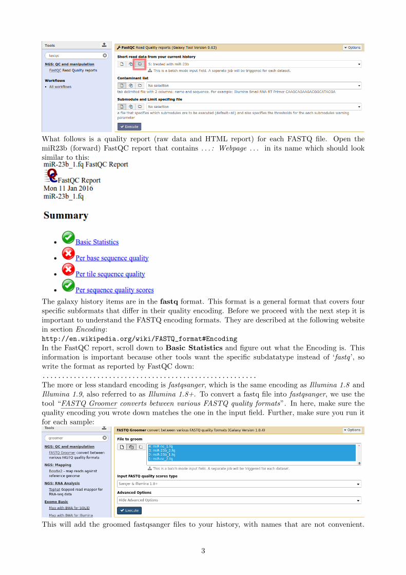
What follows is a quality report (raw data and HTML report) for each FASTQ file. Open themiR23b (forward) FastQC report that contains . . . : Webpage . . . in its name which should looksimilar to this:

The galaxy history items are in the fastq format. This format is a general format that covers fourspecific subformats that differ in their quality encoding. Before we proceed with the next step it isimportant to understand the FASTQ encoding formats. They are described at the following websitein section Encoding :http://en.wikipedia.org/wiki/FASTQ_format#Encoding

In the FastQC report, scroll down to Basic Statistics and figure out what the Encoding is. Thisinformation is important because other tools want the specific subdatatype instead of ‘fastq ’, sowrite the format as reported by FastQC down:.......................................................

The more or less standard encoding is fastqsanger, which is the same encoding as Illumina 1.8 andIllumina 1.9, also referred to as Illumina 1.8+. To convert a fastq file into fastqsanger, we use thetool “FASTQ Groomer converts between various FASTQ quality formats”. In here, make sure thequality encoding you wrote down matches the one in the input field. Further, make sure you run itfor each sample:

This will add the groomed fastqsanger files to your history, with names that are not convenient.

3

Please rename such that you can keep track of the sample name (miR23b/control) and, if you didnot use pairs, whether the reads are forward or reverse.

If we go back to the FastQC webpage report, and look in section Per base sequence quality, wesee the average quality per base for all reads. The colors green, orange and red indicate whetherthe quality is considered good, okay, or bad. As you can see, the quality drops as the sequences getlonger. It is important to realize that low quality bases will complicate alignment as well as SNPdetection, because there will be more mismatches. To improve overall the base quality of the data,we would like to:

• Trim the low quality bases from the ends

• Remove reads of which the average quality is too low

• Remove reads that are too short

A tool that covers all of this is “Sickle windowed adaptive trimming of FASTQ data”. Because wehave paired end data, we have to run it twice, once for miR-23b and once for the control. Run itwith the following settings:

After running a sickle analysis, rename the files Singletons from paired-end ... and Paired-end outputof Sickle on ... to e.g.:

for miR-23b:

– miR-23b, singletons(clean)

– miR-23b 1 (clean)

– miR-23b 2 (clean)

for control sample:

– control sample, singletons(clean)

– control sample 1 (clean)

– control sample 2 (clean)

4

If desired, you can hide the other results, such that you will get a history similar to:

As you can see, Sickle produces for every set of paired sequencing reads, a set of pairs and an extrafile with “singletons”.

• What would singletons be?

To confirm that the base quality has improved, run the FastQC again on miR-23b (clean) , andtake a look at it:

• Has the Per base sequence quality improved?

• Have the Per sequence quality scores improved?

• Why has the sequence length distribution changed?

FastQC also has a section Overrepresented sequences, indicated in red with a huge list. Apartfrom that we are using a truncated artificial dataset, it often happens in RNA-Seq data that thesesequences appear. As said before, this tool was orignally written for DNA-Seq data.

• Could you think of a reason why sequences could be overrepresented in RNA-Seq data?

2 RNA-Seq: alignment

To make more sense of the RNA-Seq data, we try to locate the detected sequences back in a referencegenome (this is often called mapping and aligning). The reference genome should represent the mostcommon sequence of the chromosomes of the human population. Please read the first paragraph (3sentences) of the following url: http://en.wikipedia.org/wiki/Reference_genome

• On how many individuals is hg19 based?

For RNA-Seq we need specialized RNA aligners, able to cope with gaps that originate from splicing.There are quite some of these aligners around. We will make use the tool “RNA STAR Gapped-readmapper for RNA-seq data”. Load the aligner, select the following settings and leave the rest ondefault, and run an alignment for miR-23b (clean) and control sample (clean). Alignment is acomputational very very heavy task so do NOT re-run it if you don’t have a goodreason, or you will have to give a treat.

5

Please rename the RNA STAR on ...: starmapped.bam to “RNA STAR on miR-23b: starmapped.bam”and “RNA STAR on control sample: starmapped.bam” or something else that makes it easy to rec-ognize. If the alignments do not have their database (also referred to as dbkey) set, change it tohg19 as follows:

To get some general alignment statistics, run the tool “Flagstat tabulate descriptive stats for BAMdatset” on miR-23b.

• How many reads are multi-mapping (‘secondary’)?

For now we have only seen FASTQ and summary files. To get an idea of what has been measuredduring the experiment, we can visualise the alignment. So, in the alignnment step we have beenlooking in hg19 where these sequences originate from, and this information is stored in the bam files.Import from the Shared Data library ( EMC Galaxy Training Materials → EMC Galaxy Training- 5: Advanced RNA-Seq Analysis ) the file “ucsc refseq.gtf ” into your history. Start the built-invisualization Trackster at one of the alignments (make sure the database is set to hg19):

6

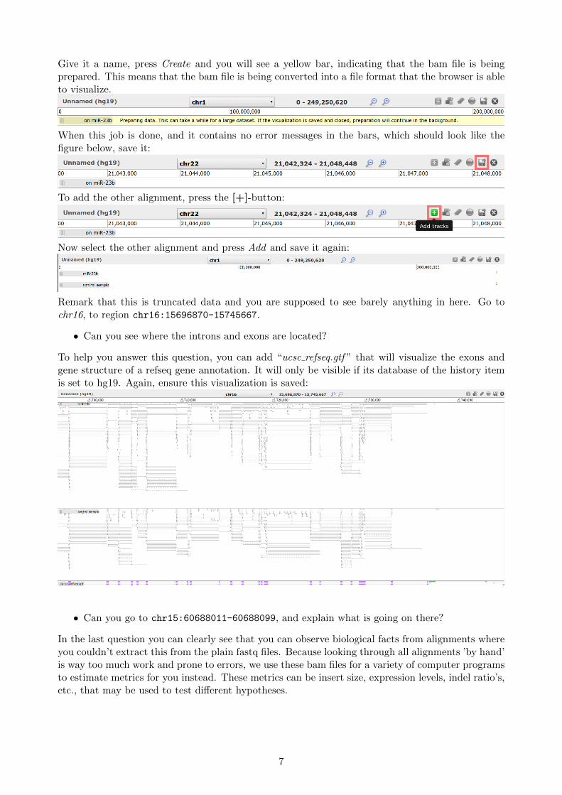
Give it a name, press Create and you will see a yellow bar, indicating that the bam file is beingprepared. This means that the bam file is being converted into a file format that the browser is ableto visualize.

When this job is done, and it contains no error messages in the bars, which should look like thefigure below, save it:

To add the other alignment, press the [+]-button:

Now select the other alignment and press Add and save it again:

Remark that this is truncated data and you are supposed to see barely anything in here. Go tochr16, to region chr16:15696870-15745667.

• Can you see where the introns and exons are located?

To help you answer this question, you can add “ucsc refseq.gtf ” that will visualize the exons andgene structure of a refseq gene annotation. It will only be visible if its database of the history itemis set to hg19. Again, ensure this visualization is saved:

• Can you go to chr15:60688011-60688099, and explain what is going on there?

In the last question you can clearly see that you can observe biological facts from alignments whereyou couldn’t extract this from the plain fastq files. Because looking through all alignments ’by hand’is way too much work and prone to errors, we use these bam files for a variety of computer programsto estimate metrics for you instead. These metrics can be insert size, expression levels, indel ratio’s,etc., that may be used to test different hypotheses.

7

3 RNA-Seq: QC/QA post alignment

Although we have ensured the base quality of our reads is high, there may be many other factorswe did not look into because they can only be deduced from the alignments. There are several toolsavailable to check for certain biases within alignments.

3.1 CollectRnaSeqMetrics

For this module, load the Shared Data ( EMC Galaxy Training Materials → EMC Galaxy Training- 5: Advanced RNA-Seq Analysis ) files:“paired-end-rna-seqmetrics.bam” and “ucsc refseq.gtf” and proceed with the tool CollectRnaSeq-Metrics as follows:

This analysis will take a while (2 minutes) and will return two files, a summary file and a PDF file.Take a look at the PDF. This pictures shows the average coverage per relative position within allgenes. As you can see there is a bias towards the 5’ end. This means that overall more reads arealigned to the 5’ end of the genes, due to library preparation. For certain types of analysis (e.g.differential isoform expression analysis) it might be important to keep this information in mind.

3.2 Inner Distance

For this module, add the Shared Data ( EMC Galaxy Training Materials → EMC Galaxy Training- 5: Advanced RNA-Seq Analysis ) file:“refseq-genes.bed” and proceed with the tool Inner Distance as follows:

The insert size is the size of the original cDNA fragment (minus the length of the mate pairs).Because RNA-seq fragments are size selected, the fragments should be within a certain range, usuallyprovided by the manufacturer. An easy way to estimate this is by calculating the insert size, thedistance in between the mates. However, due to the gaps introduced by introns in RNA-Seq, theinsert size may be much larger than the actual fragment size. The tool Inner Distance corrects forsplice junctions in the alignments and makes a plot of the distribution of the insert sizes. When

8

you take a look at the result, you will first need to understand the x-axis. If the length of the bothmates of a read is 100bp, and the insert size in the figure is 0, the length of the RNA fragment was100 + 0 + 100 = 200nt. If the insert size in the figure is 25 (mean) and both mates are 100bp inlength, the RNA fragment was 100 + 25 + 100 = 225nt. Given that the mean of the insert size is∼ 25bp, the most abundant fragment size is 225nt.

Let’s assume the manufacturer said that the fragments are size selected between 200 and 500bp.You should be able to understand why there are insert sizes smaller than 0 (insert size smaller than200) but also why they can be larger (technical and biological). There is also a small bulb of readswith an insert size even smaller than the fragment (200bp), meaning a negative fragment size. Ofcourse, this is not possible. These are reads of which the forward mate is aligned after the reverse.

4 Expression analysis advanced

4.1 Estimating gene expression

For this practical we need a RNA-seq alignments we previously made in the basic expression anal-ysis: “... miR-23b.bam”. If you did not do that practical, you can find it in the supplementarymaterial:EMC Galaxy Training Materials → EMC Galaxy Training - 5: Advanced RNA-Seq Analysis →miR-23b.bam (clean)Ensure that the file is annotated at reference genome hg19. To estimate expression in RNA-Seq,we can count the number of reads that are aligned to each gene from the list of candidate genes.Therefore you also need to import:EMC Galaxy Training Materials → EMC Galaxy Training - 5: Advanced RNA-Seq Analysis →ucsc refseq.gtfThis list is provided as a GTF/GFF file. There are a variety of tools available for counting reads.FeatureCounts is one of the faster tools and it works directly using BAM files. If you search for:“featureCounts Measure gene expression in RNA-Seq experiments from SAM or BAM files.”in the Tools menu, you can find the wrapper by the name:

Before we proceed, we would like to know whether the analysis has been performed correctly. There-fore we take a look at featureCounts’ output-summary file “featureCounts on . . . ”:

• How many reads are Assigned?

• How many reads are UnAssigned (sum of all)?

Flagstat told us the alignment has 18258 or 19493 reads in total (different versions). Please confirmwhether this matches with the total number of reads in the featureCounts summary file.

9

Table 1: results of DGE analysisReplicates Seq. Depth Significant DE genes

0 0 07rep 5M 5,000,000 ....... ?7rep 10M 10,000,000 ....... ?7rep 30M 30,000,000 ....... ?5rep 30M 30,000,000 ....... ?

If we want to look at a particular gene, we may want to truncate the large table and only showthe row with the gene of interest. To filter a tabular file we proceed with the following Galaxy tool:Filter data on any column using simple expressions:

• How many reads are aligned to DRAM1?

• Which gene has the highest read count (tip: use sort)?

4.2 Expression analysis: Low sequencing depth

In the previous exercise we found which gene had the highest read count, but what does it mean ifthis gene has a high read count all samples? To say something about expression levels, we wouldlike to say it in a context relative to other samples. Therefore, we need normalization and applystatistical testing. A popular R package that allows to do this is EdgeR, which in galaxy fits perfectlywith featureCounts.

In the following analyses you will determine the differentially expressed genes in the MCF-7-cellline between samples that have been treated with the hormone β-estradiol (E2) and those that wereleft as control [Liu et al., 2014]. The data was originally used to benchmark the statistical power ofadding replicates and does not reflect a certain disease state. In this exercise we will reproduce apart of their experiment to highlight the importance of replicates. However, it is a 2-class problemand has a similar setup as often used in cancer analysis. Before we proceed, please read the abstractof the following article: http://dx.doi.org/10.1093/bioinformatics/btt688Tip: Look up from what tissue the MCF-7 cell line originates.

For this practical we made the read count tables from featureCounts already available. We willanalyse the samples with a sequencing depth of ∼30M (full), 10M and 5M, for each replicate. Eachanalysis in this assignment will be to determine the number of differentially expressed (DE) genesand add this number to Table 1. Import the following files from data library EMC Galaxy TrainingMaterials → EMC Galaxy Training - 5: Advanced RNA-Seq Analysis :

GSE51403_expression_matrix_5M_coverage.txt

GSE51403_expression_matrix_10M_coverage.txt

GSE51403_design_matrix_subsampled.txt

10

The design matrix provides the mapping from the RNA-seq read counts per sample to the phenotypeclass each is associated with. Please take a look at file GSE51403_design_matrix_subsampled.txt

• Given that the first column lists the names of the samples and the second column the samples’corresponding condition, how many conditions does the experiment have?

4.2.1 Subsampled datasets: 5M, 7+7

For our experiment we have a 2-classes setup: a class treated with estradiol is called “E2”, and theother is called “Control”. Take one more look at the design matrix and see if you can find samplesthat belong to these classes. Go over the following steps to find the differentially expressed genesbetween “E2” and “Control” using 7 replicates per condition and 5 million reads per sample.

Note: although the design matrix contains a class description for all samples, also with 10M,25M reads and class “Unknown”, while the expression matrix contains only those for 5M reads, theedgeR wrapper will link the samples based on their sample name and proceed with those.

� Load “edgeR: Differential Gene(Expression) Analysis RNA-Seq gene expression analysis usingedgeR (R package)

� Choose Analysis type: Multigroup test and/or complex designs with e.g. blocking

� Choose Expression (read count) matrix: GSE51403_expression_matrix_5M_coverage.txt

� Choose Design matrix: GSE51403_design_matrix_subsampled.txt

� Define contrast: this is the more complicated part of the wrapper. It is effectively defining thehypothesis we want to test. This is done via a mathematical formulation in a format describedby a well known R package limma. For two class problems it is very simple: classNormal-classTreated which in our case is: Control-E2 (case sensitive!)

� Set Report differentially expressed genes to Only significant (defined by FDR cutoff) andensure the cutoff is set to 0.01.

� Don’t select additional output files and leave the rest default.

� Press [Execute]

It is always important to check whether we did not make obvious mistakes. Take a look at the file“edgeR DGE on . . . : GSE51403 design matrix.txt differentially expressed genes”. If everything iscorrect, the gene GREB1 is located in the top of the file. Please check its corresponding gene cardspage:http://www.genecards.org/cgi-bin/carddisp.pl?gene=GREB1

• Can you find on the gene cards page a regulatory factor of the gene that relates to the E2treatment?

– Hint: what was E2 again?

• Can you find on the gene cards page an association with MCF-7 cells?

– Hint: what is MCF-7 for type of cell line?

The answers to the questions should confirm that what we found with the expression analysis isin agreement with the biology behind it. If we go back to the output file, each line represents onegene, indicated by the gene symbol in the 2nd column. Because the table is ordered by FDR, thefirst column is the original position in the GTF file. The P-value, 6th column, is a probability thatrepresents the chance to find the read counts that belong to the gene, given that they are from

11

the same condition. The FDR is a multiple testing correction of the P-value and is usually usedinstead of the P-value. The lower this value, the less likely it is that the observed values are derivedfrom the same condition. Thus, differentially expressed genes will have a low FDR and P-value fordetermining significance. To distinguish between differences considered to be caused by chance orby the different conditions, we make use of a cut-off, commonly set to ≤ 0.01 or ≤ 0.05.

In edgeR we already selected to only return those genes with a FDR ≤ 0.01. Hence, the numberof lines in the history, minus 1 (header line) should give us the number of differentially expressedgenes.

• How many genes are significant differentially expressed between Control and E2?

� Please fill this in into Table 1.

4.2.2 Subsampled datasets: 10M, 7+7

In the previous analysis, the original FASTQ files used to generate the read count table, containeda total of 5.000.000 reads per sample. For the next analysis we will make use of twice the amountof raw data to see how the number of differentially expressed genes change: 10M reads per sample,7 samples per condition.

� Re-run the previous job with the rerun icon

� Replace Expression (read count) matrix: GSE51403 expression matrix 5M coverage.txtwith GSE51403 expression matrix 10M coverage.txt

• How many genes are significant differentially expressed between Control and E2? Is this moreor less than when we used 5M reads?

� Please fill this in into Table 1

4.2.3 Subsampled datasets: 30M, 7+7

In the previous analyses, the FASTQ files contained a total of 5.000.000 or 10.000.000 reads persample. The full data set contains more or less 30.000.000 raw reads per sample. Import thefollowing files from shared data:

GSE51403_expression_matrix_full.txt

GSE51403_expression_matrix_full_5x5.txt

GSE51403_design_matrix_full_depth.txt

Proceed with the following steps:

� Re-run the previous job with the rerun icon

� Replace Expression (read count) matrix: GSE51403 expression matrix 10M coverage.txtwith GSE51403 expression matrix full.txt

� Replace Design matrix: GSE51403 design matrix subsampled.txtwith GSE51403 design matrix full depth.txt

• How many genes are significant differentially expressed between Control and E2?

� Please fill this in into Table 1.

12

4.2.4 Subsampled datasets: 30M, 5+5

We did three tests with 7+7 replicates and different sequencing depths. To see what the effects areof sample replication, we should run the same analysis but use a different number of replicates. Tomodify expression matrices within Galaxy (both concatenating and removal) we can make use ofthe tool “edgeR: Concatenate Expression Matrices Create a full expression matrix”. We have usedall our replicates in the previous analyses and so we can reduce the number of replicates to 5+5 bysimply picking a subset:

This will create a truncated version of the expression matrix, only including the desired 5+5 repli-cates.

� For convenience, rename the new expression matrix to:GSE51403_expression_matrix_full_5+5_replicates.txt

� Re-run the previous edgeR DGE job with the rerun icon, make sure that the design matrix isGSE51403 design matrix subsampled.txt

� Replace Expression (read count) matrix: GSE51403 expression matrix full.txtwith GSE51403 expression matrix full 5+5 replicates.txt

� Enable the optional output: MDS-plot (logFC-method)

� Set the Output format of images to: Portable document format (.pdf)

• How many genes are significant differentially expressed between Control and E2?

� Please fill this in into Table 1.

Take a look at the MDS plot. If you want to understand all details about MDS you should dosome research online because it is a complicated mathematical operation. For now, what matters is

13

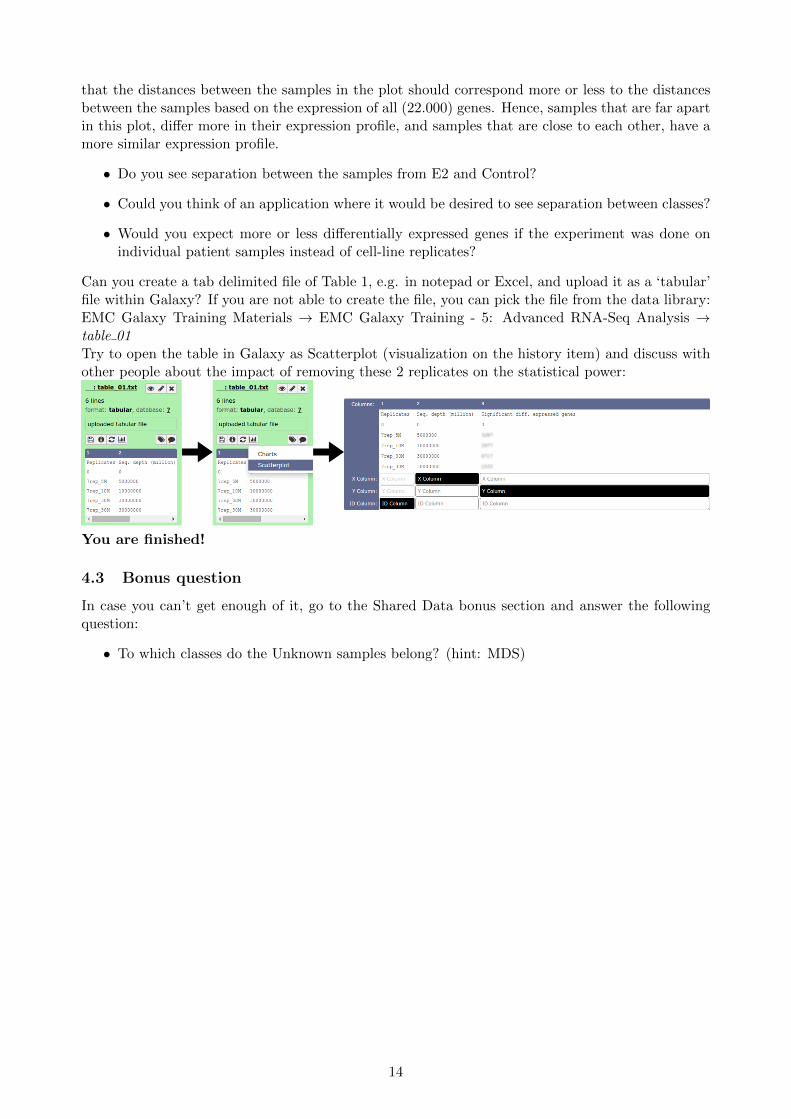
that the distances between the samples in the plot should correspond more or less to the distancesbetween the samples based on the expression of all (22.000) genes. Hence, samples that are far apartin this plot, differ more in their expression profile, and samples that are close to each other, have amore similar expression profile.

• Do you see separation between the samples from E2 and Control?

• Could you think of an application where it would be desired to see separation between classes?

• Would you expect more or less differentially expressed genes if the experiment was done onindividual patient samples instead of cell-line replicates?

Can you create a tab delimited file of Table 1, e.g. in notepad or Excel, and upload it as a ‘tabular’file within Galaxy? If you are not able to create the file, you can pick the file from the data library:EMC Galaxy Training Materials → EMC Galaxy Training - 5: Advanced RNA-Seq Analysis →table 01Try to open the table in Galaxy as Scatterplot (visualization on the history item) and discuss withother people about the impact of removing these 2 replicates on the statistical power:

You are finished!

4.3 Bonus question

In case you can’t get enough of it, go to the Shared Data bonus section and answer the followingquestion:

• To which classes do the Unknown samples belong? (hint: MDS)

14

References

Yuwen Liu, Jie Zhou, and Kevin P. White. Rna-seq differential expression studies: more sequenceor more replication? Bioinformatics, 30(3):301–304, 2014. doi: 10.1093/bioinformatics/btt688.URL http://bioinformatics.oxfordjournals.org/content/30/3/301.abstract.

15