Equity Correlation Swaps: A New Approach For Modelling...

9 November 2007

Equity Correlation Swaps: A New Approach For Modelling & Pricing14th Annual CAP Workshop on Derivative Securities and Risk ManagementNew York City

Sebastien BossuEquity Derivatives Structuring — London

2

Equity Correlation Swaps: A New Approach For Modelling & Pricing

Disclaimer

This document only reflects the views of the author and not necessarily those of Dresdner Kleinwort research, sales or trading departments.

This document is for research or educational purposes only and is not intended to promote any financial investment or security.

3


Blurb: F&D (Wiley) — S. Bossu, Ph. Henrotte

“ Finance and Derivatives teaches all of the fundamentals of quantitative finance clearly and concisely without going into unnecessary technicalities. You'll pick up the most important theoretical concepts, tools and vocabulary without getting bogged down in arcane derivations or enigmatic theoretical considerations. ”

– Paul Wilmott

$65

Seen at Columbia!

4

1. Fundamentals of index variance, constituent variance and correlation

2. Toy model for derivatives on realised variance

3. Rational pricing of correlation swaps


Agenda

5


6

1.1Realised and Implied Correlation

1.2Correlation Proxy

1.3Application: Variance Dispersion Trading



7

Realised CorrelationPair of stocks: statistical coefficient of correlation between the two time series of daily log-returnsBasket of N stocks: average of the N(N-1)/2 pair-wise correlation coefficients

Implied CorrelationPair of stocks: usually unobservableBasket of N stocks: occasionally observable through quotes on basket calls or puts from exotic desksLiquid indices: observable for listed strikes and maturities

Fundamentals of index variance, constituent variance and correlation

Realised and Implied Correlation

8

Realised Correlation Definitions (Equal Weights Assumption)

Average pair-wise (‘naive’) definition:

Canonical (econometric) definition:



∑<−

≡ji

jiNN ,Pairwise )1(2 ρρ

∑∑

<

<

<≈

jiji

jijiji

σσ

ρσσ ,

2

11

2 11⎟⎠

⎞⎜⎝

⎛≈ ∑∑

=>

=

N

ii

N

ii NN

σσ

∑

∑

=

=

−

−≡ N

ii

N

ii

N

N

1

22

2tConstituen

1

22

2Index

Canonical 1

1

σσ

σσρ

9

Implied Correlation Definition (Equal Weights Assumption)

No ‘naive’ definition (pair-wise implied correlations not observable)

Canonical (econometric) definition:

Note that the implied volatility surface translates into an implied correlation surface. We use fair variance swap strikes for σ*’s unless mentioned otherwise.



∑

∑

=

=

−

−≡ N

ii

N

ii

N

N

1

2*2

2*tConstituen

1

2*2

2*Index

*Canonical 1

1

σσ

σσρ

10






11

The previous definitions are easily generalised to arbitrary index weights

Proxy Formula: Under certain regularity conditions on the weights, residual volatility becomes negligible and we have:

Condition:


Correlation Proxy

⎪⎪

⎩

⎪⎪

⎨

⎧

≡⎟⎟⎠

⎞⎜⎜⎝

⎛⎯⎯ →⎯

≡⎟⎟⎠

⎞⎜⎜⎝

⎛⎯⎯ →⎯

+∞→

+∞→

*2

*tConstituen

*Index*

Canonical

2

tConstituen

IndexCanonical

ˆ

ˆ

ρσσρ

ρσσρ

N

N

( )No=MinWeightMaxWeight

12

Correlation (realised and implied) is thus close to the ratio of index variance to average constituent variance

This is interesting because index variance and average constituent variance can be traded on the OTC variance swap market


Correlation Proxy

VariancetConstituenAverageVarianceIndexnCorrelatio ≈

13






14

Variance Dispersion Trades Spread of variance swap positions between an index and its constituents, usually:

Long Average Constituent Variance

Short Index Variance

-

-

Exposure: long volatility, short correlation


Application: Variance Dispersion Trading

[ ][ ] 0ˆ1Cost

0ˆ1Payoff*2*

tConstituen2*

Index

2*tConstituen

2tConstituen

2Index

2tConstituen

≥−×=−=

≥−×=−=

ρσσσ

ρσσσ

15

By underweighting the constituents’ leg with a factorβ = ρ* < 1, several benefits are obtained:

Vega-NeutralityOn trade date, if constituent variance goes up 1 point and implied correlation is unchanged, index variance would go up by ρ* points and the P&L is: β x 1pt – ρ* pts = 0

Zero cost

Straightforward p&l decomposition


Application: Variance Dispersion Trading

]ˆˆ[CostPayoffL&P *2tConstituen

Zero

ρρσβ

−×=−=

0Cost 2*Index

2*tConstituen =−= σσβ

16

2. Toy Model for Derivatives on Realised Variance

17

2.1Realised Variance: A Tradable Asset

2.2Toy Model for Realised Variance

2.3Application: Volatility Swap

2.4Parameter Estimation

2.5Model Limitations



18

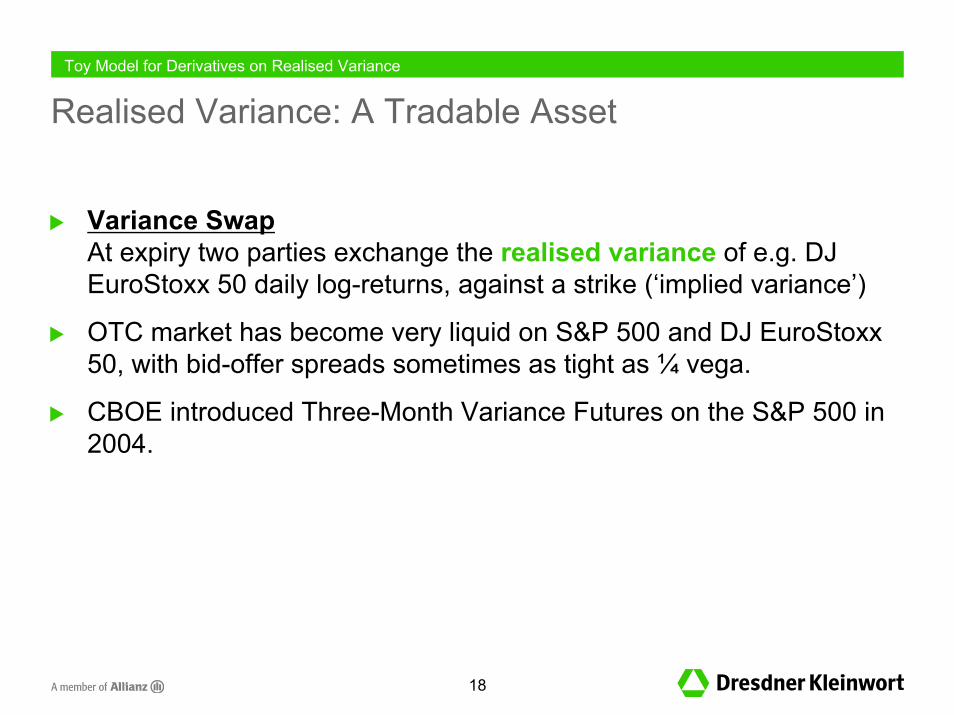
Variance SwapAt expiry two parties exchange the realised variance of e.g. DJ EuroStoxx 50 daily log-returns, against a strike (‘implied variance’)

OTC market has become very liquid on S&P 500 and DJ EuroStoxx50, with bid-offer spreads sometimes as tight as ¼ vega.

CBOE introduced Three-Month Variance Futures on the S&P 500 in 2004.

Toy Model for Derivatives on Realised Variance

Realised Variance: A Tradable Asset

19








20

Which Model for Realised Variance?

Fischer Black: ‘I start with the view that nothing is really constant. Volatilities themselves are not constant, and we can’t write down the process by which the volatilities change with any assurance that the process itself will stay fixed. We’ll have to keep updating our description of the process.’

‘Studies of Stock Price Volatility Changes’, cited in Fischer Black and the Revolutionary Idea of Finance, P. Mehrling, John Wiley & Sons, 2005


21

Popular models (in particular Heston) for volatility or variance focus on the instantaneous, non-tradable volatility

Other approaches (Dupire, Buehler) focus on the variance swap curve, which is tradable; or a fixed-term variance asset (Duanmu, Carr-Sun)

Toy ModelStraightforward modification of Black-Scholes where the volatility of the variance asset vt linearly collapses as we approach its expiry T:


Toy Model for Realised Variance

tt

t dZT

tTvdv −

= ω2Volatility of volatility

22

vT is the price of the variance asset at expiry and coincides withrealised variance over the interval [0, T]

v0 is the fair price of the variance asset which can be observed on the variance swap market or calculated through the replicating portfolio of puts and calls

v0 = E( vT )

The terminal distribution of vT is lognormal, making closed-form formulas for European derivatives on realised variance easy to derive


Toy Model for Realised Variance

23








24

Payoff = √vT – Kvol

With the Toy Model we find:

Numerical example: v0 = 202 = 400, T = 1, ω = 50% → Kvol ≈ 19.2


Application: Volatility Swap

⎟⎠⎞

⎜⎝⎛−= TvKvol

20 6

1exp ω

Variance Swap Strike

Quadratic Adjustment

25








26

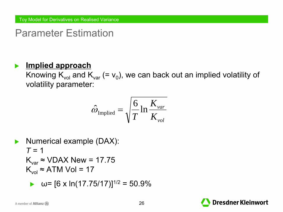
Implied approachKnowing Kvol and Kvar (= v0), we can back out an implied volatility of volatility parameter:

Numerical example (DAX):T = 1Kvar ≈ VDAX New = 17.75Kvol ≈ ATM Vol = 17

ω= [6 x ln(17.75/17)]1/2 = 50.9%


Parameter Estimation

vol

var

KK

Tln6ˆImplied =ω

27

Historical approaches

Classical: e.g. reconstitute historical time series of fixed-maturity variance prices (vt)0≤t≤T, on a rolling basis (computationally intensive)

Break-even historical analysis: e.g. find the quadratic adjustment which, on average, neutralises the P&L of an arbitrageur trading the spread between variance and volatility swaps


Parameter Estimation

28

If volatility and variance swaps had the same strike, there would be an arbitrage:

Thus Kvol < Kvar. Consider an arbitrageur who executes on dates m = 1,2,...,M a series of normalised spread trades: BUY 1/(2Km

2) units of variance at Km and SELL (1/Km) units of volatility at Km/γ:

where Rm denotes realised volatility between dates m and m + τ


Parameter Estimation: Break-Even Analysis

∑=

⎥⎦

⎤⎢⎣

⎡⎟⎟⎠

⎞⎜⎜⎝

⎛ −−⎟⎟⎠

⎞⎜⎜⎝

⎛ −=

M

m m

mm

m

mm

KKR

KKRlp

12

22 )(2

/ γ

p/l

σ0Graph of σ- 20

Graph of2022022

×−σ

20

29

Assuming p/l = 0 and solving for γ, we find:

This is the break-even quadratic adjustment. The corresponding theoretical volatility of volatility parameter is then given as:



Γ≡⎥⎥⎦

⎤

⎢⎢⎣

⎡⎟⎟⎠

⎞⎜⎜⎝

⎛ −−=

−

=∑ ˆ

211

1

1

2M

m m

mm

KKR

Mγ

Γ= ˆln6ˆImplied Tω

30

Results for the Dow Jones Euro Stoxx 50 index, using monthly trading dates m between 2000 and 2005



1.029

1.064 1.0631.059

1.043

1.051

42%

61%

87%

123%

145%

109%

1.02

1.03

1.04

1.05

1.06

1.07

0 3 6 9 12 15 18 21 24

Maturity (months)

20%

50%

80%

110%

140%

170%

Index break-even quadratic adjustment (lhs) Index theoretical vol of vol (rhs)

1 year

31








32

The usual Black-Scholes limitations apply: constant volatility of volatility, no transaction costs, continuous hedging.

Specific limitations:

Log-normal assumption inconsistent with additivity of variance: the toy model is not suitable to model the variance swap curve, even with a time-dependent ω

No joint dynamics with the asset price process: the toy model does not explain/take into account the equity skew

Consistency with vanilla option prices not considered.


Model Limitations

33

3. Rational Pricing of Correlation Swaps

34

3.1Correlation Swaps

3.2Fair Value


3.4Dynamic Hedging Strategy




35

Correlation SwapAt maturity two parties exchange the average pair-wise realised correlation between e.g. the DJ EuroStoxx 50 constituents, against a strike.

OTC market, not very liquid. Introduced in early 2000’s as a means for equity exotic desks to recycle their correlation parametric risk.

Typically correlation swaps trade at a strike which is 5 to 15 points below implied correlation.

Rational Pricing of Correlation Swaps

Correlation Swaps

36

Correlation Swap Payoff:

The pricing and dynamic hedging of this payoff is non-trivial. However we can simplify the problem using the Proxy formulas:

which is the ratio of two tradable assets: index variance and average constituent variance


Correlation Swaps

Pairwise,)1(2 ρρ =−

≡ ∑< ji

jiNNPayoff

2tConstituen

2Index

Canonical ˆσσρρ =≈≈Payoff

37

1-month realised correlation


How Good Is The Proxy?

0%

10%

20%

30%

40%

50%

60%

70%

80%

Jan-

00

Jan-

01

Jan-

02

Jan-

03

Jan-

04

Jan-

05

Jan-

06

Jan-

07

Realised Correl Proxy Canonical Correl Average Pairwise Correl (Weighted)

38

24-month realised correlation


How Good Is The Proxy?

0%

10%

20%

30%

40%

50%

60%

70%

80%

Jan-

00

Jan-

01

Jan-

02

Jan-

03

Jan-

04

Jan-

05

Jan-

06

Jan-

07

Realised Correl Proxy Canonical Correl Average Pairwise Correl (Weighted)

39


3.2Fair Value






40

Define vtI as the index variance asset, vt

S as the average constituent variance asset, with the following forward-neutral dynamics:

Define as the payoff to replicate.


Two-factor Toy Model

[ ]ttt

t

tt

t

dZdWT

tTvvd

dWT

tTvdv

2SS

S

II

I

12

2

χχω

ω

−+−

=

−=

Volatility ofconstituent volatility

Correlation betweenindex and constituent vols

ρ̂S

I

=≡ TT v

vcT

Volatility ofindex volatility

41

After calculations we find the fair value of the correlation proxy :

The implied-to-fair correlation adjustment factor is given as:

Note: For the adjustment factor to be above 1 (i.e. correlation swap strike below implied correlation, as observed on OTC markets), the correlation between index and constituent volatilities must be >> 0


Fair value

( ) ⎥⎦⎤

⎢⎣⎡ −== T

vvcEc T χωωω IS

2SI

0

I0

0 34exp)(

AdjustmentFactor

ρ̂

( ) ⎥⎦⎤

⎢⎣⎡ −= T

c2

SIS0

*0

34exp

ˆωχωωρ

Implied Correlation*0ρ̂

42


3.2Fair Value






43

Break-even estimation of the volatility of constituent volatility of the DJ EuroStoxx 50 (2000—2005):



1.021

1.042

1.050 1.051

1.033

1.029

89%

123%

101%

70%54%

39%1.02

1.03

1.04

1.05

1.06

1.07

0 3 6 9 12 15 18 21 24

Maturity (months)

20%

50%

80%

110%

140%

170%

Constituent break-even quadratic adjustment (lhs) Constituent theoretical vol of vol (rhs)

1 year

44

Adjustment factor for various correlation of volatilities χ:


Implied-to-fair correlation adjustment factor: numerical examples

Mat. Index volatility of volatility ..

Constituent volatility of volatility …

Adjust. Factor

(χ = 0.6)

Adjust. Factor

(χ = 0.7)

Adjust. Factor

(χ = 0.8)

Adjust. Factor

(χ = 0.9)

Adjust. Factor (χ = 1)

1m 144.7% 123.4% 0.951 0.970 0.990 1.009 1.030

2m 122.6% 101.2% 0.940 0.966 0.993 1.021 1.049

3m 109.2% 88.9% 0.933 0.964 0.995 1.028 1.062

6m 86.5% 69.9% 0.920 0.957 0.997 1.038 1.081

12m 60.5% 54.1% 0.880 0.919 0.960 1.003 1.047

24m 41.5% 38.6% 0.869 0.906 0.946 0.987 1.031

SωIω

45


3.2Fair Value






46

0.. SS

II

SSII =−=Δ+Δ=Π tt

tt

t

tttttt v

vcv

vcvv

Hedging coefficients (deltas):

Hedging portfolio:


Dynamic Hedging Strategy

SS

II

t

tt

t

tt v

cvc

−=Δ=Δ

Short vega-neutral variance dispersion[Weight ratio between the constituent and index legs is equal to ‘correlation’]

Zero cost

Short constituentvariance

Long index variance

47


3.2Fair Value






48

In addition to the limitations of the one-factor Toy Model, the two-factor Toy Model is not entirely arbitrage-free as a result of the unconstrained evolution of index and constituent variance price processes:

The two-factor Toy Model allows for vtI > vt

S !

Also the two-factor Toy Model relies on the assumption that constituent stocks and their weights are static, which is only reasonable for short maturities.


Model limitations

49

Model probability of terminal realised correlation cT > 1, for an initial implied correlation of 50%, ad hoc implied volatility of volatility parameters ω, and various correlation of volatilities χ:


Model limitations

95%confidence

level0%2%4%6%8%

10%12%14%16%

0 3 6 9 12 15 18 21 24Maturity (months)

χ = 0.5 χ = 0.55 χ = 0.6 χ = 0.65χ = 0.7 χ = 0.75 χ = 0.8 χ = 0.85χ = 0.9 χ = 0.95 χ = 1.0

1 year

50

A correlation swap on an equity index can be quasi-replicated by dynamically trading vega-neutral variance dispersions at zero cost

Using a straightforward extension of Black-Scholes, we find that the fair strike of a correlation swap is equal to Implied Correlation multiplied by an adjustment factor which depends on volatility of index volatility, volatility of constituent volatility and correlation between index and constituent volatilities.

Using a parameter estimation methodology which relies on few historical observables, we obtain numerical results supporting the intuitive idea that the adjustment factor should be close to 1.


Conclusion

51

FundamentalToy Model needs to be made entirely arbitrage-free.

Practical

Fair value of other correlation measures (e.g. canonical or average pair-wise measures)

Free-float weights, changes in index composition

NumericalMore sophisticated parameter estimations, over longer historicalperiods and in other markets


Further research

52

References & Bibliography

53

Consistent Variance Curve Models, H. Buehler, Finance and Stochastics, Vol. 10, No 2 / April 2006.

A New Approach for Option Pricing Under Stochastic Volatility,P. Carr and J. Sun, Bloomberg LP, Working paper (2005)

Robust Replication of Volatility Derivatives, P. Carr and R. Lee, Bloomberg LP & University of Chicago, Working paper (2005)

Rational Pricing of Options on Realized Volatility, Z. Duanmu, Global Derivatives & Risk Management Conference, Madrid (2004)

Arbitrage Pricing with Stochastic Volatility, B. Dupire, Proceedings of AFFI Conference in Paris, June 1992.Self-referencing (available at math.uchicago.edu/~sbossu)

Fundamental relationship between an index’s volatility and the average volatility and correlation of its components, with Y. Gu, JPMorgan Equity Derivatives, Working paper (2004)

A New Approach For Modelling and Pricing Correlation Swaps, Dresdner Kleinwort report, Working paper (2007)


References & Bibliography

http://math.uchicago.edu/~sbossu/

Equity Correlation Swaps: A New Approach For Modelling...

Documents

Transcript of Equity Correlation Swaps: A New Approach For Modelling...