FIW, a collaboration of WIFO (www.wifo.ac.at), wiiw (www.wiiw.ac.at) and WSR (www.wsr.ac.at)

FIW – Working Paper

Equilibrium Real Effective Exchange Rates and Real Exchange Rate Misalignments:

Time Series vs. Panel Estimates

Oliver Hossfeld

We follow the behavioral equilibrium exchange rate approach by Clark and MacDonald (1998) to derive equilibrium real effective exchange rates and currency misalignments for the US and its 16 major trading partners. We apply cointegration and panel cointegration techniques to derive fully country-specific measures of misalignment and measures based on panel estimates. We formally test the forecast performance of pooled vs. heterogeneous estimators over a hold-back period and find that pooling the data delivers more accurate forecasts in the vast majority of cases although the implicit long-run homogeneity restriction is statistically rejected. This is especially remarkable, since we have given the heterogeneous estimator an ’unfair’ advantage by choosing the country-specific model (of up to 21 possible ones) with the best out-of-sample performance prior to comparing it to two final panel specifications. Robustness of the results is supported by recently introduced cross-sectionally augmented panel unit root tests by Pesaran (2007) and bootstrapped error correction-based panel cointegration tests by Westerlund (2007), as well as different estimators. While we find strong evidence for the Balassa-Samuelson-effect, the evidence for other commonly hypothesized fundamentals is weak. JEL-Code: C22, C23, F31, F37 Keywords: behavioral equilibrium, exchange rate, real exchange rate misalignment, panel cointegration, CIPS test, cross-sectional dependence, exchange rate forecasts, exchange rate fundamentals

Address: Sparkassen-Finanzgruppe-Chair of Macroeconomics, HHL – Leipzig Graduate School of Management, Jahnallee 59, 04109 Leipzig, Germany. Email: oliver.hossfeld@hhl.de. I thank conference participants in Berlin, Magdeburg, and Vienna for helpful comments and discussions.

Abstract

The author

FIW Working Paper N° 65 December 2010

Equilibrium Real Effective Exchange Rates

and Real Exchange Rate Misalignments:

Time Series vs. Panel Estimates

Oliver Hossfeld∗

September 2010

Abstract

We follow the behavioral equilibrium exchange rate approach byClark and MacDonald (1998) to derive equilibrium real effective ex-change rates and currency misalignments for the US and its 16 ma-jor trading partners. We apply cointegration and panel cointegrationtechniques to derive fully country-specific measures of misalignmentand measures based on panel estimates. We formally test the forecastperformance of pooled vs. heterogeneous estimators over a hold-backperiod and find that pooling the data delivers more accurate forecastsin the vast majority of cases although the implicit long-run homogene-ity restriction is statistically rejected. This is especially remarkable,since we have given the heterogeneous estimator an ’unfair’ advan-tage by choosing the country-specific model (of up to 21 possible ones)with the best out-of-sample performance prior to comparing it to twofinal panel specifications. Robustness of the results is supported byrecently introduced cross-sectionally augmented panel unit root testsby Pesaran (2007) and bootstrapped error correction-based panel coin-tegration tests by Westerlund (2007), as well as different estimators.While we find strong evidence for the Balassa-Samuelson-effect, theevidence for other commonly hypothesized fundamentals is weak.

JEL Classification Numbers: C22, C23, F31, F37

∗Address: Sparkassen-Finanzgruppe-Chair of Macroeconomics, HHL - LeipzigGraduate School of Management, Jahnallee 59, 04109 Leipzig, Germany. Email:oliver.hossfeld@hhl.de. I thank conference participants in Berlin, Magdeburg, and Viennafor helpful comments and discussions.

1 Introduction

According to the behavioral equilibrium exchange rate (BEER) approach in-troduced by Clark and MacDonald (1998) real (effective) exchange rates aredetermined by certain fundamentals such as the real interest rate differen-tial, net foreign assets or relative productivity advances. Until the end ofthe 1990s authors mostly relied on time series analysis to estimate such rela-tionships and derive currency misalignments (among others, Faruqee, 1995,Clark and MacDonald, 1998, and MacDonald, 1998). Recently, more authorshave taken a panel perspective (for instance Kim and Korhonen, 2005, Villav-icencio, 2006, Bénassy-Quéré et al., 2009, and Ricci et al., 2008).1 However,using time series techniques to estimate equilibrium exchange rates remainspopular.2

Bénassy-Quéré et al. (2009) find BEER estimations to be ’quite robust’with regard to the choice of relative productivity proxy, countries includedin the panel (G20 vs. G7, respectively non-G7 countries), the numeraire cur-rency, and to small changes of the sample period. However, results from Mac-Donald and Dias (2007) show that parameter estimates differ substantiallyacross countries,3 and for each country individually, depending on whetherresults are obtained from time series or panel estimations. The differencesare either attributable to true parameter heterogeneity among the countries,to imprecise estimates due to the low number of observations in the timeseries dimension, to a biased pooled estimator in the case of true parameterheterogeneity, or most probably a combination of them.4

So, should we put more trust in the individual time series estimates or inthe pooled estimates when calculating equilibrium exchange rates and deriv-ing currency misalignments? The answer to this question bears importantpolicy implications. Consider for instance the recently revitalized debatesabout a possibly emerging/already existing ’currency war’. Among others,a proper assessment whether a country’s currency is manipulated, requires

1Notable exceptions are Chinn and Johnston (1997), Chinn (2000), and Gagnon (1996)who (also) apply panel techniques.

2More recent contributions using time series techniques include Alstadt (2010), Atsushi(2006), Nilsson (2004), and Maeso-Fernandez et al. (2002).

3The estimated coefficients for the trade balance to GDP ratio vary between -177.77for Japan and -1.34 for the US in their study.

4In the case of true parameter heterogeneity across countries, country-specific (i.e.heterogeneous) time series estimations are theoretically the first choice, because the pooledestimator is biased if the implicit (parameter) homogeneity restriction is rejected (Maddalaet al., 1997). However, if the time series are too short, estimates can be highly inaccurateand estimated coefficients be even incorrectly signed (Baltagi et al., 2008 and Maddala etal., 1997).

knowledge of the relationship between (perhaps ’manipulated’) fundamentalsand exchange rates. If the methodology used to estimate such relationshipsis unreliable, we neglect an important ingredient to a well-grounded discus-sion. A country joining a currency union is yet another example, becausea fair conversion rate for the currency needs to be established. Unreliableestimates of the proper rate, and, as a consequence, a possibly severe cur-rency misalignment, could unnecessarily give rise to inflation or deflation inthe accession country and even slow down economic growth in the case ofprolonged misalignments (Edwards and Savastano, 1999). Furthermore, thefair value of a currency is not only of interest to central bankers and govern-ment agencies, but also to the private sector (Edwards and Savastano, 1999),since current deviations from the ’fundamentally justified’ value may servean information variable for future exchange rate movements.

Rapach and Wohar (2004) analyze whether the monetary exchange ratemodel performs better in forecasting bilateral nominal exchange rates if theunderlying parameter estimates are obtained from panel estimations as com-pared to country-by-country estimations. They find the pooled estimator todeliver a better forecasting performance, although the underlying poolabilityhypothesis is statistically rejected. With regard to the empirical modeling ofreal equilibrium exchange rates, Égert (2004) notes that

’Across different papers, the whole gamut of fundamentals isused, and, as a corollary, the outcome is sensitive to which partic-ular fundamentals are included in the estimated model. The useof different fundamentals may be a result of different theoreticalframeworks or may simply reflect ad hoc choices.’

So, whereas the choice of fundamentals is predetermined by the choice of themonetary exchange rate model in Rapach and Wohar (2004), there is at leastsome degree of arbitrariness with respect to the selection of determinants inthe class of models we consider.5 Notwithstanding the arbitrariness observedin the relevant literature, it may well be that the importance of certaindeterminants in explaining real effective exchange rate movements differsacross countries.6

To assess the reliability of time series versus panel approaches in estimat-ing equilibrium exchange rates we therefore estimate up to 21 specifications

5Commonly chosen determinants include net foreign assets, measures of relative pro-ductivity differentials, relative terms of trade, measures of the openness of a country, therelative stock of government debt and real interest rate differentials. Less frequently, alsothe real oil price (especially for emerging market countries) has been considered (Amanoand van Norden, 1998).

6However, it may be questionable whether one should call these country-specific deter-minants ’fundamental ’ determinants of real exchange rates.

2

for each of the included countries (depending on the univariate time prop-erties of the considered determinants) and twelve panel specifications over arestricted sample from 1986Q1 to 2002Q4, and then compare the relative ac-curacy of conditional forecasts obtained from these models over a hold-backperiod from 2003Q1 to 2006Q4.7

We focus on two ’extreme’ estimators: the fully country-specific (i.e. het-erogeneous) dynamic OLS (DOLS) estimator and the pooled DOLS esti-mator.8 Because we impose homogeneity of the cointegration slopes in thepooled estimations, we formally check whether this restriction holds.9 How-ever, even a rejection of the poolability null would not necessarily mean thatthe obtained pooled estimates are worthless. It may well be that the ’benefitsof higher estimation precision’ outweigh the ’costs of bias’ as also the resultsfrom Rapach and Wohar (2004) suggest.10

While we follow the Behavioral Equilibrium Exchange Rate (BEER) ap-proach by Clark and MacDonald (1998) to estimate ’fundamentally justi-fied’ values of specific currencies, a number of other concepts with similaracronyms have been proposed – most notably, the Fundamental EquilibriumExchange Rate (FEER) approach by Williamson (1994a) and the NaturalReal Exchange Rate (NATREX) approach by Stein (1995). Whereas thelatter two concepts are normative and involve ad-hoc judgments on the sizeof central parameters, the BEER approach (which will be introduced in thenext section) is rather statistical and free of normative elements. Due tothe high number of publications dealing with equilibrium exchange rates andthe vast number of competing concepts, a literature survey on equilibriumexchange rate would necessarily have to be very selective. Instead we refer tothe excellent survey articles by MacDonald (2000), Driver and Wren-Lewis(1998), Driver and Westaway (2005), Williamson (1994b, and 2009).

This paper is structured as follows: In section 2 we shortly introducethe BEER concept. In section 3 we present the data, its sources and howthe data has been transformed. In section 4 we give a short overview of

7Methodologically similar, Baltagi et al. (1997 and 2000) compare the out-of-samplepredictive performance of homogeneous versus various heterogeneous estimators for thedemand for gasoline respectively cigarettes.

8The DOLS estimator accounts for potentially endogenous regressors as opposed tothe simple OLS estimator. Disregarded endogeneities would be another potential sourceof bias (simultaneity bias) we avoid by using DOLS.

9To check the robustness of the results, we alternatively use the modified OLS (FMOLS)estimator as well as the respective group mean estimators, where the slope homogeneityrestrictions are not imposed.

10As a ’safety net’ we additionally apply the group-mean DOLS estimator by Pedroni(2004), which gives consistent estimates of the average cointegration slopes, regardlesswhether the long-run parameters are homogeneous or heterogeneous across countries.

3

first and second generation panel unit root tests, which will then be applied– together with simple univariate unit root tests for each of the countriesindividually – to examine the order of integration of the involved time series.After a short methodological introduction, we will conduct the country-by-country estimations in section 5. We then turn to the panel analysis. Insection 6 we present two kinds of panel cointegration tests, which will thenbe applied to test for long-run relationships among various subsets of thevariables. In section 7 we conduct conditional forecasts over the hold-back-period to assess the relative forecast accuracy of both models, which may beregarded as an informal out-of-sample stability analysis. Based on the resultsof this exercise, we choose a preferred specification, which is then reestimatedover the full sample to derive equilibrium real effective exchange rates andcurrency misalignments. Finally, section 8 concludes the article.

2 The BEER Concept and the Choice of Fun-

damentals

In this section we present the origins of the BEER concept and shortly presentits theoretical foundations. For extensive surveys on the BEER concept andrelated concepts (such as CHEER, FEER, ITMEER, NATREX) we refer toDriver and Westaway (2005) and MacDonald (2000). The BEER conceptarised from the discomfort with Purchasing Power Parity (PPP) as a reason-able explanation for the observed real exchange rate behavior. Shocks to thereal exchange rate have been found to be too persistent to be accordant withPPP (the so called ’PPP-puzzle’ (Rogoff 1996)), ’typical’ half-life estimatesto shocks to PPP being around four years. The very slow mean reversionspeeds therefore provide at best support for an ’ultra-long-run’ concept ofequilibrium exchange rates (Edwards and Savastano, 1999). Often even nosignificant mean reversion has been found.11 From a theoretical point of viewPPP has been criticized as a concept for the determination of the equilib-rium exchange rate, because it ignores the role of capital flows and any realdeterminants of the real exchange rate (MacDonald, 2000). The aim of theBEER approach is on the one hand to be better able to relate the observedexchange rate behavior to movements in certain other variables, and on theother hand to correct the theoretical shortcomings of PPP as a method fordetermining equilibrium exchange rates. A general problem with respect toequilibrium exchange rates is that they are unobservable. Consequently, es-timated long-run relationships between the observed real exchange rate and

11Surveys can be found in MacDonald (2000), and Taylor and Taylor (2004).

4

the fundamentals are assumed to equal the equilibrium exchange rate towardswhich the real exchange rate adjusts (Égert, 2004).12

The BEER approach is derived from the real interest parity condition(thereby accounting for capital flows) and – assuming that the expectedfuture real exchange rate is a function of fundamental variables – also takesinto account real determinants.

Following, we briefly present the theoretical concept based on MacDonald(2000):

Starting point is the risk-adjusted real UIP condition (which is completelydisregarded in the concept of PPP):

∆qet+k = −(rt − r∗t ) + λt (1)

where qt denotes the real exchange rate, e the expectations operator, rt theex-ante real interest rate and λt a risk premium. The real exchange rate isexpressed in foreign currency units per unit of domestic currency, so that anincrease represents a (real) appreciation of the domestic currency.

Rearranged for the real exchange rate we have:

qt = qet+k + (rt − r∗t)

− λt (2)

As the expected real exchange rate is unobservable, this relationship ishard to test empirically; qet+k is therefore interpreted as the fundamental orlong-run component of the real exchange rate, denoted qt. Substituting into(2) yields:

qt = qt + (rt − r∗t )− λt (3)

In a popular stock-flow consistent model of exchange rate determination,Faruqee (1995) identifies the stock of net foreign assets and a set of exogenousvariables as fundamental determinants of the equilibrium (or long-run) ex-change rate. In an extension of this model, Alberola et al. (1999) decomposethe real exchange rate into an external and an internal real exchange rate,both of which relate to one specific theory of exchange rate determination.The external rate is defined as the ratio of the price of domestic relative toforeign tradable goods and is connected to the notion of external balance,whereas the internal rate is defined as the relative price of non-tradable goodsto tradable goods within each country and connected to the notion of inter-nal balance. The equilibrium exchange rate is the one at which external

12Funke (2005) describes the BEER as the ’data-determined systematic component ofthe exchange rate in the medium and long run’.

5

and internal balance are achieved, i.e. the tradable goods market is cleared(and the desired net foreign asset position achieved), and there is no excessdemand for non-tradable goods.13

A short intuitive motivation for the inclusion of specific fundamentals,which are hypothesized to account for the time-varying value of the realexchange rate, and which are theoretically founded by one model or anotheror are commonly used in the literature in an ad-hoc style is given below.For model-specific derivations we refer to Frenkel and Mussa (1985), Faruqee(1995), Chinn and Johnston (1996), and Alberola et al. (1999).

Net Foreign Assets

The effect of a country’s net foreign asset position on the equilibriumexchange rate is expected to be positive. According to standard in-tertemporal macroeconomic models, a higher stock of net foreign lia-bilities causes interest payments to increase, which ultimately have tobe paid for by improved trade balances. In order to generate higher netexports, the competitiveness of the respective country has to improve,necessitating a depreciation of the real exchange rate.

Productivity Bias

According to the well-known Balassa-Samuelson (BS) hypothesis, rel-atively larger increases in productivity in the tradable goods sectorcompared to the non-tradable goods sector are connected with a realappreciation of the domestic currency. The rise in relative productivityof the tradable goods sector causes wages in the tradable goods sectorto increase. Wage equalization across the sectors ensures that wagesin the non-tradable sector also increase (which is not compensated forby an accordant rise in productivity). Consequently, the overall pricelevel is higher and we observe a real appreciation of the equilibriumexchange rate.

Government Consumption

According to Genberg (1978), Bergstrand (1991), and MacDonald (1998)the presence of non-traded goods can furthermore introduce a demandside bias, if the income elasticity of demand for non-traded goods is

13The BEER approach therefore includes the same set of fundamentals as the FEERapproach. However, the latter implies the calibration of a sustainable current account andtherefore follows a normative approach.

6

greater than 1. As government consumption is primarily devoted tonon-traded goods (compared to private consumption), a rise in govern-ment consumption (or a redistribution of income towards the govern-ment) therefore increases the relative price of non-tradable goods andcauses the equilibrium exchange rate to appreciate.14 On the otherhand, a growing budget deficit might also cast doubt on the sustain-ability of fiscal policy, destabilize the economy and lead to a real de-preciation (Melecký and Komárek, 2007).

Terms of Trade

When traded goods are imperfect substitutes, their relative price mightchange due to changes in supply and demand caused by changes in un-derlying determinants such as consumer preferences or differing growthrates (Edwards, 1989 and Nilsson, 2004). Import and export price in-dices will be affected differently across countries, thereby changing therelative terms of trade. The effect of terms of trade shocks to the realexchange rate is however ambiguous (Melecký and Komárek, 2007). Onthe one hand, an increase in the (relative) prices of a country’s exportgoods gives rise to a positive substitution effect, because domestic pro-ducers shift their production towards tradable goods. This will causewages in this sector to increase relative to the ones in the non-tradablegoods sector. If wages subsequently equalize across the sectors, thiswill drive up the overall price level and thereby lead to a real appreci-ation. However, at the same time a positive wealth effect (reflected inthe improved current account) may generate higher demand for non-tradable goods and necessitate a real depreciation to restore internalbalance (Melecký and Komárek, 2007).

Openness

Openness is often introduced as a proxy for trade liberalization. Ahigher degree of openness (i.e. a removal of trade restrictions) maylower domestic prices and cause a real depreciation (Goldfajn andValdes, 1999 and Elbadawi, 1994). As emphasized by Dufrenot andYehoue (2005) this variable is however more likely to be relevant for de-veloping or emerging countries than for industrial ones, since we wouldnot expect the degree of openness to vary a lot for these countries. We

14See Chinn (1997) for a formal implementation of this argument in a real exchange ratemodel.

7

therefore think that its influence should, with the exception of China,be fairly limited in our set of countries.

3 Data Description

Our panel consists of the US and 16 of its major trading partners: Australia,Belgium, Canada, China, France, Germany, Ireland, Italy, Japan, Korea,Mexico, Netherlands, Spain, Sweden, Switzerland and the UK. These coun-tries either make up a a significant part of US trade, or are an issuer ofa major currency, i.e. their currency circulates widely outside the countryof issue. Some countries have not been included in the panel due to toomuch missing data for some of the relevant variables (Taiwan, Singapore,Hong Kong, Malaysia, and Brazil). The sample consists of quarterly datafrom 1986Q1 to 2006Q4. For some variables and countries, data interpola-tion techniques are applied to obtain quarterly data. All variables exceptfor the net foreign asset to GDP ratio, the trade balance to GDP ratio andthe openness ratio are measured relative to the trade-weighted average ofthe respective variables of the trading partner countries. Trading weights areconstant throughout the sample and are taken from Bayoumi et al. (2005).15

The trade-weights for all included countries (rescaled so that they sum to 1)are presented in table 9. Although the countries have been chosen with spe-cial regard to the US, table 1 shows that all countries included in the panelmake up a large proportion of trade for each of the other countries (rangingfrom 69 percent for Sweden to 90 percent for Mexico). So we believe thatthe results are meaningful for all countries.

Table 1: Sum of Trade Weights of Partner Countries

AUS BEL CAN CHN FRA GER IRL ITA JPN

78% 89% 75% 78% 70% 84% 74% 70% 72%

KOR MEX NLD ESP SWE CHE UK US

74% 90% 77% 77% 69% 80% 77% 76%

Data is taken from IMF International Financial Statistics (IFS) unless stateddifferently. Exchange rates are defined in indirect quotation so that an in-crease in the exchange rate implies an appreciation of the domestic currency.Annual Consumer Price Inflation (CPI) for China has been obtained from the

15Reference period for the calculation of these weights is 2002/2003 and weights takeinto account direct bilateral competition as well as third-market competition.

8

National Bureau of Statistics of China, interpolated to quarterly frequencyand updated with growth rates from IFS.16 The real effective exchange rate(reer) is calculated as the geometric average of the 16 bilateral nominal ex-change rate indices multiplied with the respective CPI ratio. Data on netforeign assets is taken from Lane and Milesi-Ferretti (2007) and updated byaccumulating current account balances. To scale the variables, we divideby GDP to obtain the net foreign asset to GDP ratio (nfa). Alternatively,we also use the trade balance to GDP ratio (tb), which is available at ahigher frequency.17 For China and Ireland annual GDP data is converted toquarterly frequency for some periods.18 Relative terms of trade (tot) are de-fined as the ratio of the domestic export unit value and the domestic importunit value divided by the geometrically weighted (using the same weights asabove) foreign ratios. The relative productivity differential (ntt) is proxiedby the ratio of the domestic consumer price index (CPI) to the domesticwholesale price index (WPI) divided by the geometrically weighted foreignratios (see Faruqee, 1995, Gagnon, 1996, Alberola, 1999), and Bénassy-Quéréat al. (2009).19

The real interest rate is calculated as the difference between the nominallong-term interest rate and the percentage change of the CPI index comparedto its value in the same quarter in the year before. Nominal long-term interestrates are partly taken from sourceOECD. For China the lending rate is usedinstead, and for Mexico the 3-month treasury bill rate is taken until 1989Q4.20

The real interest rate differential (rird) is then calculated as the differencebetween the domestic real interest rate and the trade-weighted arithmeticaverage real interest rate of the trading partners. Relative government con-sumption textbf(gov) is defined as the domestic government consumption toGDP-ratio relative to the trade-weighted ratios of government consumptionto GDP-ratios of the trading partners. Openness (open) is defined as theratio of the sum of exports and imports (in absolute values) to GDP. Whilereer, gov and tot are expressed in logarithmic terms, nfa, tb, open and rirdare measured as fractions of 100.

16We use the cubic-spline interpolation technique. However, results are robust to chang-ing the interpolation technique.

17tb has first been introduced as an alternative for nfa by MacDonald and Dias (2007). Apositive long-run relationship between nfa and reer implies a negative long-run relationshipbetween tb and reer.

18For Ireland until 1996Q4, for China until 1998Q4.19This proxy is surely not undisputed (see for instance Schnatz and Osbat (2003). How-

ever, first, it is in contrast to other (similarly disputable) indicators widely available, andsecond, results by Bénassy-Quéré et al. (2009) indicate that results are largely robust.

20One missing value for Mexico for 1986Q3 is proxied by the average of the precedingand the succeeding quarter.

9

4 (Panel) Unit Root Tests

As noted in the introduction we put ourselves once fully in the position of atime series econometrician, and once in the position of a panel econometri-cian. We also follow this approach when assessing the order of integration ofthe involved time series.

Time series econometricians usually apply the familiar Dickey-Fuller typeunivariate unit root tests to assess the order of integration of certain time se-ries. Because the tests are fairly standard we do not introduce them here. Weconduct two types of tests, the well-known augmented Dickey Fuller (ADF)test as well as the Dickey-Fuller generalized least squares (DFGLS) test pro-posed by Elliott et al. (1996).21 To save space, neithter the test results arereported here, but can be obtained from the author upon request. Later,we will conduct country-by-country tests for cointegration for all differentsubsets of variables, in which only variables are included that are tested tobe I(1) in the country-by-country unit root tests.

Univariate unit root tests are known to have low power to reject thenull hypothesis of a unit root, if the respective time series contains a ’nearunit root’, i.e. the autoregressive parameter is close to but lower than one.Increasing the dimension of the panel from N = 1 (where N is the numberof cross section units) to N > 1 lowers the probability of committing a type2 error. However, a number of complications arise in the presence of morethan one cross section unit. This is reflected in the large number of panelunit root tests which have been developed. Whereas the rejection of the nullhypothesis of a unit root is trivial to interpret if N = 1, it is less obvious forN > 1. Rejection could either mean that the respective series is stationaryfor all cross units of the panel, or that it is stationary for a fraction of thecross units included in the panel only.

We implement three panel unit root tests: The Levin-Lin-Chu (2002)(LLC) test, the Im-Pesaran-Shin (2003) (IPS) test, and the Pesaran (2007)CIPS (cross-sectionally augmented IPS) test. We will only comment on themain differences among these three panel unit root tests. For a comprehensiveformal treatment of these and other panel unit root tests (including thederivation of the tests and test statistics, and some Monte Carlo evidence)see Breitung and Pesaran (2005), which we also draw upon in this shortsurvey. For an overview of second generation panel unit root tests see Hurlinand Mignon (2007).

The tests we consider differ in two main aspects: first, whether a common

21Elliot et al. (1996) and Ng and Perron (2001) show that this test is more powerfulwhen an unknown trend and/or mean is present.

10

autoregressive process is assumed under the alternative hypothesis, and sec-ondly, how potential cross-sectional dependencies are dealt with. The LLCand the IPS test belong to the so-called ’first generation’ of panel unit roottests, while the Pesaran CIPS test is one of several recently proposed ’sec-ond generation’ tests. While the latter test takes into account cross-sectionaldependencies, the former two do not (or only to a very limited extent byincluding common time dummies in the test regressions). While the LLCand IPS tests are still the most commonly applied ones, several studies haveshown that the empirical size of a panel unit root test can vastly divergefrom the nominal size if cross-sectional dependencies are disregarded (see forinstance Banerjee et al., 2005).

Before we more carefully address the issue of cross-sectional dependencies,we have a closer look at the LLC and IPS tests. The LLC test starts fromthe following pooled ADF test regression (lags of the differenced dependentvariable are disregarded for simplicity):

∆yi,t = αi + δit+ θt + ρiyi,t−1 + εi,t, (4)

The test allows for some degree of heterogeneity by including country fixedeffects (αi), country-specific deterministic (time) trends (δit) and dampensthe effects of cross-sectional dependencies by including common time dum-mies (θt). However, ρi is obtained by running a pooled OLS regression, i.e.ρi = ρ for all countries. The null and alternative hypotheses of the LLC testare H0 : ρi = 0∀i, respectively Ha : ρi = ρ < 0∀i. We see that the LLC test isvery restrictive under the alternative hypothesis by assuming that the seriesfollows the same autoregressive process for all cross units. This ’drawback’is addressed by the IPS test, which is a group-mean test. The alternativehypothesis is that Ha : ρi < 0 for at least one i. In contrast to the LLCtest, where the estimate of ρ is obtained by running a pooled regression, ρi isestimated for each cross unit individually before a group-mean test statistic,t, is obtained though averaging the individual t-statistics. The test is lessrestrictive because ρi may be different for different i under HA. Both testsconsidered so far can only handle cross-sectional dependencies to a very lim-ited degree (by including common time dummies). However, this approachis not suitable if the pair-wise cross-section covariances of the error terms aredifferent across the individual series (Pesaran, 2007). Pesaran (2007) there-fore proposes a generalized IPS test, which allows a common factor to havedifferent effects on each cross unit.22

22Banerjee et al. (2005) show that the empirical size of panel unit root tests is muchhigher than the nominal level in case there are cross-unit cointegration relationships whichare not taken into account in the respective critical values. In other words, it is likely that

11

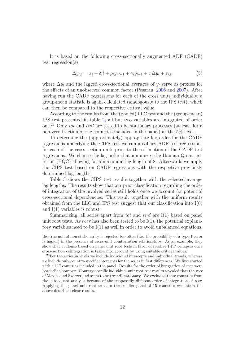
It is based on the following cross-sectionally augmented ADF (CADF)test regression(s)

∆yi,t = αi + δit+ ρiyi,t−1 + γiyt−1 + ςi∆yt + εi,t, (5)

where ∆yt and the lagged cross-sectional averages of yt serve as proxies forthe effects of an unobserved common factor (Pesaran, 2006 and 2007). Afterhaving run the CADF regressions for each of the cross units individually, agroup-mean statistic is again calculated (analogously to the IPS test), whichcan then be compared to the respective critical value.

According to the results from the (pooled) LLC test and the (group-mean)IPS test presented in table 2, all but two variables are integrated of orderone.23 Only tot and rird are tested to be stationary processes (at least for anon-zero fraction of the countries included in the panel) at the 5% level.

To determine the (approximately) appropriate lag order for the CADFregressions underlying the CIPS test we run auxiliary ADF test regressionsfor each of the cross-section units prior to the estimation of the CADF testregressions. We choose the lag order that minimizes the Hannan-Quinn cri-terion (HQC) allowing for a maximum lag length of 8. Afterwards we applythe CIPS test based on CADF-regressions with the respective previouslydetermined lag-lengths.

Table 3 shows the CIPS test results together with the selected averagelag lengths. The results show that our prior classification regarding the orderof integration of the involved series still holds once we account for potentialcross-sectional dependencies. This result together with the uniform resultsobtained from the LLC and IPS test suggest that our classification into I(0)and I(1) variables is robust.

Summarizing, all series apart from tot and rird are I(1) based on panelunit root tests. As reer has also been tested to be I(1), the potential explana-tory variables need to be I(1) as well in order to avoid unbalanced equations.

the true null of non-stationarity is rejected too often (i.e. the probability of a type 1 erroris higher) in the presence of cross-unit cointegration relationships. As an example, theyshow that evidence based on panel unit root tests in favor of relative PPP collapses oncecross-section cointegration is taken into account by using suitable critical values.

23For the series in levels we include individual intercepts and individual trends, whereaswe include only country-specific intercepts for the series in first differences. We first startedwith all 17 countries included in the panel. Results for the order of integration of reer wereborderline however. Country-specific individual unit root test results revealed that the reer

of Mexico and Switzerland seem to be (trend)stationary. We excluded these countries fromthe subsequent analysis because of the supposedly different order of integration of reer.Applying the panel unit root tests to the smaller panel of 15 countries we obtain theabove-described clear results.

12

Table 2: First Generation Panel Unit Root Test Results

REER NFA NTT TB

LLC level −0.67 −0.08 −0.33 1.871st diff. −21.30∗∗∗ −2.48∗∗∗ −19.88∗∗∗ −30.87∗∗∗

IPS level −1.20 0.05 1.57 −1.211st diff. −20.76∗∗∗ −12.62∗∗∗ −19.43∗∗∗ −32.84∗∗∗

TOT GOV OPEN RIRD

LLC level −1.86∗∗ 0.84 2.79 −2.18∗∗

1st diff. −30.33∗∗∗ −33.28∗∗∗ −21.22∗∗∗ −21.94∗∗∗

IPS level −4.10∗∗∗ 1.50 1.65 −3.20∗∗∗

1st diff. −29.52∗∗∗ −32.76∗∗∗ −23.06∗∗∗ −26.69∗∗∗

Note: Reported are the t-statistics for the IPS test and the t∗-statistics forthe LLC test. We allow for individual deterministic trends and constants,and series are demeaned. ***, **, and * denote significance at the 1, 5,and 10% level, respectively.

Table 3: CIPS Second Generation Panel Unit Root Test Results

REER NFA NTT TB

CIPS level −2.58 −2.37 −2.29 −2.36avg. lags 1.53 3.13 1.00 1.00

CIPS 1st diff. −5.92∗∗∗ −3.23∗∗∗ −5.80∗∗∗ −5.877∗∗∗

avg. lags 0.47 2.13 0.33 0.60

TOT GOV OPEN RIRD

CIPS level −2.99∗∗∗ −2.03 −1.70 −2.78∗∗

avg. lags 0.80 0.47 0.73 1.87CIPS 1st diff. −6.11∗∗∗ −5.94∗∗∗ −5.66 −5.62∗∗∗

avg. lags 0.60 0.27 0.73 1.87

Note: We report the t-statistics. Avg. lags denotes the average lag lengthof the underlying CADF test regressions. ***, **, and * denote significanceat the 1, 5, and 10% level, respectively.

13

This implies that we will test for long-run relationships among subsets ofreer, nfa, tb, ntt, gov and open only, and disregard tot and rird in the panelcointegration analysis. We however do not generally disregard these variablesin the country-by-country cointegration analyzes. Based on the country-by-country univariate unit root tests tot appears to be non-stationary for someof the countries. This result contrasts with the IPS and CIPS-test results,which maintain that tot is not stationary for any of the cross units. It maybe regarded as a typical example for the previously noted lower power ofindividual unit root tests compared to panel unit root tests in rejecting anear unit root. However, as we consider the situation of a time series analystwho only takes into account information based on regressions for a singlecross unit, this knowledge would not be available to him. In line with theprevious argument, the fraction of nonstationary series is larger according tothe country-by-country unit root tests. Consequently, the number of specifi-cations which need to be tested for cointegration is also larger compared tothe panel analysis.

5 Country-by-Country Analysis

5.1 Tests for Cointegration and Estimation Methodol-

ogy

We (primarily) apply the DOLS estimator to estimate the long-run relation-ships among subsets of variables. We choose this specific estimator for tworeasons: First, it can easily be applied in (nonstationary) panel regressionsas well. By choosing the equivalent panel estimator we narrow down the rea-sons for possibly different results, because different estimation results cannotbe attributed to a different estimation technique then. Secondly, the DOLSestimator accounts for potential endogeneities among the variables.24

DOLS has been introduced by Saikkonen (1991) and Stock and Watson(1993) and extended to panel analysis by Kao and Chiang (1997). By incor-porating leads and lags of the first differences of the regressors endogenousfeedback effects from the dependent variable to the regressors are absorbed.In contrast to OLS, the DOLS estimator is therefore consistent, even if regres-sors are endogenous. Without a cross-sectional dimension, a DOLS(k1,k2)regression can be written as:

24The regular OLS estimator is biased if regressors are not weakly exogenous.

14

Yt = β0 +n

∑

i=1

βiXi,t +n

∑

i=1

k2∑

j=−k1

γi,j∆Xi,t−j + εt,

where k1 and k2 denote the numbers of leads and lags, which can be chosenaccording to various information criteria.

To check which of the estimated regressions are spurious and which formlong-run relationships, we perform Engle-Granger cointegration tests. Criti-cal values for the Engle-Granger cointegration tests are calculated from theresponse surface function presented in MacKinnon (1990). Using these ob-tained critical values we check whether the residuals from the supposed long-

run relationship, υt = Yt − β0 −

n∑

i=1

βiXi,t, are indeed stationary. If not,

then the null of no cointegration cannot be rejected and the relationship isspurious.

In order to check whether the results are robust against using another es-timation technique, we additionally present results obtained from fully mod-ified OLS (FMOLS) regressions. The FMOLS estimator also accounts forendogenous regressors, but in contrast to the DOLS estimator, the bias cor-rection is obtained in a non-parametric way.

5.2 Estimation Results

So far we have neither presented country-by-country unit root test nor coin-tegration test results, since this would consume too much space due to thelarge number of series/specifications. Instead, we directly report the DOLSand FMOLS estimation results in table 2.11 for the specifications for whichthe following three conditions are fulfilled: First, all series included in each ofthe specifications have to be I(1) according to the individual countries’ unitroot test results, secondly, the residual of the cointegration vector has to bestationary, and thirdly, there has to be mean reversion in the error correctionmodel (ECM) representation so that the regression can be interpreted as areal exchange rate equation. Consequently, for the large number of remainingspecifications which are not reported here, at least one of the three conditionsis not fulfilled. Only DOLS(1,1) results are reported, because the inclusionof further leads and lags changed the point estimates only marginally. Thereported standard errors of the DOLS regressions are heteroscedasticity andautocorrelation consistent (HAC).

Overall, the results are very mixed. First, for four countries (AUS, ESP,FRA, and UK) we do not find any specification fulfilling all the above cri-teria. Secondly, we do not find a single specification (containing the same

15

set of explanatory variables) for the remaining countries, either pointing to-wards true heterogeneity of the different BEER equations or to impreciseestimates due to the relatively low number of observations for each of thecross-section units. Stationary combinations including nfa are only obtainedfor four countries (CHN, JPN, IRE, and NLD) and the estimated signs arecounterintuitive.25 Also tb is only included and significant in a very few cases(CAN, CHN, and US).26 Based on the country-specific estimation results wecould therefore doubt their economic significance. However, we abstain fromdrawing further conclusions at this point, and will instead reconsider the roleof nfa and tb in the context of the subsequent panel analysis.

Whereas evidence in favor of these commonly hypothesized determinantsis at best weak, we find strong evidence in favor of the BS effect. It isincluded in all specifications and the sign and size of the coefficient estimatesare plausible (a one percent increase in ntt is connected with a 0.65 percentto 2.67 percent appreciation of the domestic currency).

Evidence for the other determinants is mixed again. tot is included inonly three specifications (CAN, CHN, and SWE), which is not surprisingagainst the background of the panel unit root tests, according to which tot isstationary, whereas reer is nonstationary. For the above three specificationsthe estimated coefficient of tot is always positive thereby providing weakevidence in favor of the substitution effect dominating the wealth effect.While open is included in the specifications of six countries (CAN, GER,JPN, KOR, NLD, and SWE) the respective point estimates vastly differ(estimated coefficients range from -0.35 for CHN to about -6.43 for JPN).

gov has a significantly negative impact on reer in three countries (CAN,CHN, and IRL). This lends some support to the hypothesis that concernsabout fiscal sustainability dominate the effects of (relatively) higher govern-ment spending on non-traded goods in these countries. In the case of JPN,the relationship among gov and reer is significantly positive.

The FMOLS results are in most cases very similar to the DOLS(1,1)results. Consequently, our results do not seem to depend on the choice ofthe estimator.

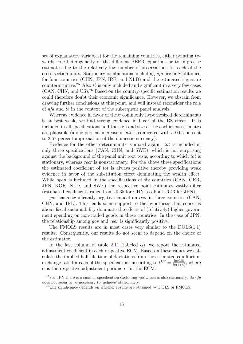
In the last column of table 2.11 (labeled α), we report the estimatedadjustment coefficient in each respective ECM. Based on these values we cal-culate the implied half-life time of deviations from the estimated equilibriumexchange rate for each of the specifications according to t1/2 = ln(0.5)

ln(1+α), where

α is the respective adjustment parameter in the ECM.

25For JPN there is a smaller specification excluding nfa which is also stationary. So nfa

does not seem to be necessary to ’achieve’ stationarity.26The significance depends on whether results are obtained by DOLS or FMOLS.

16

The half-life time varies between less than 2 quarters and about 5 quar-ters for most of the specifications, which is a dramatic improvement overpreviously estimated half-life times implied by PPP, and an even larger ’im-provement’ compared to our own finding that reer is I(1) implying that thereis no significant mean reversion (and therefore no evidence supporting PPP)at all.27 Notwithstanding the favorable results in terms of adjustment speedstowards equilibrium, the obtained country-by-country results are very mixedin general, and one should therefore not overemphasize these findings, be-cause they may be based on imprecise estimates.

Summarizing the country-by-country results, it is highly difficult to findsensible and robust specifications for the regarded countries. This may eitherbe attributed to the low power of cointegration tests in small samples (68observations), and, closely related, to imprecise estimates, or, trivially, tothe non-existence of sensible cointegration relationships among the variables.However, there is one exception: We obtain sensible results with respect tontt, which is estimated quite robustly across units with the expected positivesign and by and large reasonable coefficient estimates. This lends strongsupport to the BS-effect.

6 Panel Analysis

6.1 Tests for Panel Cointegration and Estimation Method-

ology

There is a close analogy between panel cointegration tests and panel unit roottests. Some of the tests are based on group-mean estimates, others on pooledestimates. Some take into account cross-sectional dependencies, while othersdo not. We will apply two representative (bundles of) panel cointegrationtests: the very popular Pedroni (2004) test(s) for panel cointegration and therecently introduced test(s) by Westerlund (2007). A comprehensive surveyon panel cointegration tests is provided by Breitung (2005).

Since the Pedroni panel cointegration test (2004) is residual-based, it canbe regarded as a panel equivalent of the Engle-Granger test for cointegrationcommonly applied in time series analysis. Pedroni proposes seven tests, ofwhich three are group-mean tests and the remaining four are pooled tests(with the respective differing alternative hypotheses). A detailed discussionof each individual test statistic is outside the scope of this paper and we referto Pedroni’s (2004) original article for further details. Similarly as in the case

27Only in GER and ITA adjustment to shocks is much slower (the implied half-life timeis about 3 years for Germany and almost 6 years for Italy).

17

of the Johansen test for cointegration, short-run parameters and country-specific deterministic trends are filtered out in two first stage regressions.By doing so the Pedroni test allows for country-specific short-run effectsand different lag-lengths in the test-regressions (in contrast to the formerlyheavily applied test by Kao, 1999). In general, it can be regarded as asign of robustness if several of the different test statistics lead to the sametest decision, because evidence based on Monte Carlo simulations has shownthat the various test statistics perform differently depending on the paneldimension and the assumed data generating process.

The error-correction based test by Westerlund (2007) does not only allowfor various forms of heterogeneity, but also provides p-values which are robustagainst cross-sectional dependencies via bootstrapping.28 In short, it is testedwhether the null of no error correction can be rejected (either for the wholepanel or for a non-zero fraction of the cross units depending on whether apooled or group-mean estimation is performed). If the null can be rejected,there is evidence in favor of cointegration.

While two of the four tests are panel tests with the alternative hypothesisthat the whole panel is cointegrated (HP

A : αi = α < 0 for all i), the othertwo tests are group-mean tests which test against the alternative hypothesisthat for at least one cross-section unit there is evidence of cointegration(HG

A : αi < 0 for at least one i). For the group-mean test statistics, the errorcorrection coefficient is estimated for each cross-section unit individually, andthen two average statistics (denoted Gt, respectively Gα) are calculated.29 Inthe pooled tests, the series of each cross-section unit are ’cleaned’ first (ofdynamic nuisance parameters, unit-specific intercepts and/or trends), beforethe conditional (or ’cleaned’) panel error correction model is estimated toobtain a common α estimate, which is checked for significance.

6.2 Estimation Results

While we apply the Pedroni test to search for long-run relationships amongtwelve different subsets of variables, the Westerlund test is only applied tothe specifications for which the Pedroni tests provide strong evidence in favorof cointegration.30 The number of subsets is determined by the results of the

28For a description of the respective STATA procedure see Persyn and Westerlund(2008).

29For more details on the test-statistics and their derivation see the above reference.30Banerjee et al. (2004) show that panel cointegration tests can be largely oversized in

the presence of cross-unit long-run relationships. Not accounting for such relationshipstherefore makes it more likely to obtain a finding in favor of cointegration, which maybe false. It is therefore sensible to apply the Westerlund test which accounts for cross-

18

Table 4: Pedroni Panel Cointegration Test Results

Specification M1 M2 M3 M4 M5 M6

REER REER REER REER REER REERNFA NFA NFA NFA

TB TBNTT NTT NTT NTT NTT NTT

GOV GOV GOVOPEN OPEN

Panel Testsν-stat. 1.13 1.16 0.92 1.04 1.14 0.68ρ-stat. 0.00 0.37 0.56 0.78 −0.79 0.03t-stat. (ADF) −0.80 −0.59 −0.47 −0.42 −1.66 −1.05t-stat. (PP) −1.35∗ −1.12 −0.83 −0.02 −2.32 −0.92

Group Mean Testsρ-statistic 1.26 1.43 1.63 1.75 0.59 1.45t-stat. (PP) 0.04 0.04 0.21 0.16 −0.79 −0.06t-stat. (ADF) −1.11 −0.96 −0.75 0.78 −2.34∗∗∗ −0.75

Specification M7 M8 M9 M10 M11 M12

REER REER REER REER REER REER

TB TBNTT NTT NTT NTT NTT NTT

GOV GOV GOVOPEN OPEN OPEN OPEN

Panel Testsν-stat. 1.04 0.90 1.67∗∗ 1.05 1.12 0.86ρ-stat. 0.15 0.65 −1.68∗∗ −0.63 −0.47 0.01t-stat. (ADF) −0.80 −0.56 −2.18∗∗ −1.45∗ −1.12 −0.95t-stat. (PP) −1.35∗ −0.97 −2.40∗∗∗ −1.65∗∗ −1.31∗ −0.87

Group Mean Testsρ-statistic 1.24 1.72 −0.08 0.61 0.73 1.14t-stat. (PP) −0.14 0.08 −1.26 −0.69 −0.36 −0.19t-stat. (ADF) −1.12 −1.17 −1.86∗∗ −1.57∗ −0.76 −0.62

Note: ***,** and * denote the significance levels of 1, 5, and 10%.

19

Table 5: Westerlund Panel Cointegration Test

Statistic Value Z-value p-value Robustp-value

Gt -2.515 -3.180 0.001 0.010Ga -9.452 -1.644 0.050 0.030Pt -7.708 -2.114 0.017 0.098Pa -7.580 -2.922 0.002 0.023

Note: Note: Optimal lag/lead length determinedby Akaike Information Criterion with a maximumlag/lead length of 3. Width of Bartlett-kernel win-dow set to 3. We allow for a constant, but no de-terministic trend in the cointegration relationship.Number of bootstraps to obtain bootstrapped p-values which are robust against cross-sectional de-pendencies set to 400.

panel unit root tests, according to which only reer, nfa, tb, ntt, and open areI(1), and additionally by our own requirement that ntt is included in all testedsubsets. While this may seem somewhat arbitrary, we believe it is sensibleto do so against the background of the country-by-country estimation resultsproviding strong evidence of the BS-effect.

One result is particularly remarkable: Evidence in favor of cointegrationis the strongest when only ntt is considered as a regressor (see table 4). Inthis case, 5 of the reported 7 statistics point towards the presence of a coin-tegrating relationship among the variables. If the specification additionallyincludes gov we can only reject the null of no cointegration in 3 of 7 cases. Forthree other specifications only one of the statistics points towards cointegra-tion, for the remaining 7 specifications we find no evidence of cointegrationat all, although the former specifications are restricted versions of the latter.The results imply that while the linear combination in M9 forms an irre-ducible cointegration relationship, the others do not. In contrast, the linearcombinations seem ’less stationary’ once further variables are included. Intable 5 we present the Westerlund test results for M9. In the last columnwe present the bootstrapped p-values, which account for cross-sectional de-pendencies. They point towards reer and ntt being cointegrated, therebysupporting the overall Pedroni test result. According to three of the fourtest statistics we can reject the null of no significant error correction at the

sectional dependencies only to the specifications for which the Pedroni test points towardscointegration.

20

Table 6: Pooled DOLS Estimates

M1 M5 M7 M9 M10 M11

NFA −0.09∗∗∗

(0.02)TB −0.83∗∗∗ −0.29∗∗

(0.08) (0.11)NTT 1.15∗∗∗ 0.98∗∗∗ 0.75∗∗∗ 1.18∗∗∗ 1.31∗∗∗ 0.76∗∗∗

(0.10) (0.10) (0.08) (0.10) (0.09) (0.08)GOV −0.32∗∗∗

(0.07)OPEN −0.38∗∗∗ −0.43∗∗∗

(0.06) (0.05)

Poolability 10.56∗∗∗ 15.51∗∗∗

Note: Driscoll and Kraay standard errors in brackets. ***,** and * denotethe significance levels of 1, 5, and 10%, respectively. The null hypothesis ofthe Roy-Zellner test is poolability/slope homogeneity across countries.

5%-level, while one rejects only at the 10% level.31

As stated above, we also focus on the DOLS estimator in our panel anal-ysis. First we run pooled DOLS regressions allowing for two-way fixed effects(country fixed effects and common time effects). The pooled is estimatoris only unbiased if the cointegration slopes are equal across countries. Wetherefore formally test whether the poolability hypothesis is not rejected afterhaving performed the estimations.

We report Driscoll and Kraay (1998) standard errors, which account forwithin-group correlation, heteroscedasticity and cross-sectional correlation.32

Because the inclusion of common time effects does not substantially changethe point estimates of the other coefficients, we only present the point esti-mates without common time dummies included.

DOLS(1,1) results for the restricted sample are presented in table 6 forthe specifications, for which at least one of the reported Pedroni test statis-tics is in favor of rejecting the null of no cointegration, however, given theresults of the panel cointegration tests we focus on specifications 9 and 10in the subsequent analysis. The findings suggest that only ntt is necessary

31According to the asymptotic p-values in the second-last column, we can reject the nullof no cointegration in all cases.

32We used the STATA module ’xtscc’ by Hoechle (2007) to provide robust standarderrors.

21

Table 7: Group Mean DOLS and FMOLS Estimates

M1 M9 M10

DOLS FMOLS DOLS FMOLS DOLS FMOLSNFA −0.02 0.02

(−0.64) (−0.20)NTT 1.43∗∗∗ 1.42∗∗∗ 1.24∗∗∗ 1.21∗∗∗ 1.31∗∗∗ 1.42∗∗∗

(13.07) (12.57) (16.38) (14.16) (18.73) (14.70)GOV −0.30∗∗∗ −0.30∗∗∗

(−2.93) (−2.66)

Note: ***,** and * denote the significance levels of 1, 5, and 10%, respectively.

to achieve stationarity.33 The obtained point estimate of ntt is significantlypositive and of reasonable size (with a point estimate of 1.18). A value largerthan the hypothesized value of 1 seems reasonable as our rough proxy is likelyto capture other demand side effects as well. Accordingly, the panel resultssupport the results obtained in the country-by-country analysis with respectto the relevance of ntt.

However, we have to be cautious in interpreting the results, because wehave to reject the null hypothesis of poolability across countries according tothe Roy-Zellner test (Roy, 1959, Zellner, 1962, and Baltagi, 2005), which isreported for specifications 9 and 10 at the bottom of table 6.34

Baltagi (2005) and Baltagi and Griffin (1997) suggest to choose a prag-matic approach. Instead of disregarding the pooled model if the poolabilityrestriction is rejected, they propose to base the decision of whether pool-ing is advantageous or not on the out-of-sample forecast performance of theheterogeneous models vs. the pooled model. We will follow their advice.

Before we do so in the subsequent section, we provide group-mean DOLSand FM-OLS results of the cointegration slopes for three different models(M1, M9, and M10 ). Group-mean DOLS and FMOLS estimators have beenintroduced by Pedroni (2004). The advantage of these estimators is thatthey provide consistent estimates of the average cointegration slopes evenif the slopes are in fact different across countries. We choose the above

33It contrast to all other combinations reer and ntt form a so-called irreducible cointe-gration relationship (Davidson, 1999).

34We only test the slope coefficients of the original regressors in levels (ntt, respectivelyntt, gov) for homogeneity across countries, not the ones from the lags and leads of theirfirst differences. See Vaona (2008) on how to implement this test in STATA.

22

models for two reasons: First, evidence of cointegration has been strongestfor M9 and M10. Secondly, because nfa has commonly been included inBEER equations we want to check whether its numerically small coefficientestimate obtained in the pooled regression may be due to omitted variablebias in M1.35 Estimation results are presented in table 7.

We observe that the estimate of the cointegration slope coefficient of ntthardly changes in our preferred specification M9 (from 1.18 in the pooledDOLS regression to 1.24 and 1.21 in the group-mean FMOLS and DOLSregressions, respectively). The same holds for M10, where the coefficientof gov either does not change much if we apply the group mean DOLS orFMOLS estimator instead of the pooled estimator (-0.32 compared to -0.30).It is furthermore notable that the coefficient estimate of nfa is even smallerand insignificant in the group mean regressions (see M1 ). Consequently,the small coefficient estimate of nfa in M1 in the pooled case may even betoo large. Based on these findings and the country-by-country estimationresults, nfa does not seem to be a fundamental determinant of reer.36 It istherefore hard to argue that the depreciation of the USD in current yearsis a direct response to the growing US external liabilities. However, thissurely does not mean that nfa does not have any influence on the reer atall. If one is on the one hand willing to accept the theoretically appealingproposition that net foreign liabilities ultimately have to be repaid and onthe other hand empirical evidence in favor of a linear long-run relationship isat most weak, this may raise concerns of a (non-linear) sudden adjustmentonce certain thresholds are reached. We leave such a threshold-analysis aswell as a robustness check of our results with respect to other countries andsamples to further research.

7 Conditional Forecasts

Based on the results of the panel cointegration tests, the plausibility of thecoefficient estimates, and the limited impact of other variables on reer, panelspecifications M9 and M10 are the only panel specifications which we con-sider in our conditional forecasting exercise over the reserved part of thesample (2003Q1 to 2006Q4). Their forecasting performances are compared

35By pooling the data, we implicitly introduce this form of bias if the slope homogeneityrestriction does not hold.

36Panel results of Villavicencio (2006) with regard to the the coefficient of nfa are verysimilar. He considers two different panel estimators (DOLS and the pooled mean groupestimator), but only according to one (PMGE) nfa enters significantly into a long-runrelationship with reer. Additionally, the estimated coefficients are also very small (around0.06) and very similar to our estimates.

23

with the ones from the fully country-specific time series models. To assessthe relative forecasting performance of the competing models, we conductconditional forecasts in the reserved part of the sample. The estimated coef-ficients are held fixed at their in-sample values for the whole ex-post forecastevaluation horizon. The interpretation of the results warrants some cautionhowever. Forecasting errors may either be attributed to the instability of theestimated parameters or to true misalignments of the REER with respectto its estimated equilibrium value. But we believe that the objective of theBEER approach to match the observed real exchange rate behavior as closelyas possible, should also remain the objective out-of-sample. We therefore re-gard a model as superior to another if it provides a better out-of-samplefit.37 To assess the relative predictive performance of two competing models(within a specific sample) we calculate their relative root mean squared error(RMSE). Table 8 shows the relative RMSE for different pairs of models. Inthis table we only consider the fully-country specific model delivering the bestfit over the hold-back period and our preferred panel specifications M9 andM10.

As the predictions based on both panel specifications are very similar,we subsequently only comment on the more parsimonious specification M9.According to the relative RMSE, panel specification M9 delivers a betterforecasting performance for 8 out of 11 countries, the only exceptions be-ing BEL, CHN and JPN. To test whether the forecasting performance issignificantly better, we conduct Diebold Mariano tests, which test the nullhypothesis of equal expected forecast accuracy against the alternative of dif-ferent forecasting ability across models. As only conditional forecasts areconducted, the classical Diebold Mariano statistic can be used and no cor-rection for possible autocorrelation among the residuals has to be made sincethere are no overlapping forecasts. The panel delivers significantly betterforecasts for 8 countries (see table 9), the fully country-specific models aresignificantly better in just two cases (BEL and JPN). This results is remark-able, since we have given the heterogeneous estimator an ’unfair’ advantageby choosing the country-specific model with the best out-of-sample fit priorto comparing it to the performance of the two panel specifications.

Based on these results, we think that pooling the data provides more ro-bust estimates of the impact of underlying fundamentals on the (observed)real exchange rate, although the poolability hypothesis is statistically re-jected. Given the better performance of the pooled estimator in terms ofRMSE performance, we recommend its use when calculating equilibrium ex-

37Considering the limited size of the reserved sample, we certainly cannot be sure,whether this result is robust or simply due to the presence of extraordinary shocks.

24

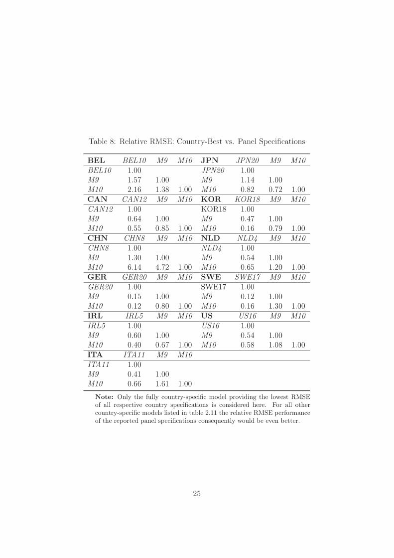
Table 8: Relative RMSE: Country-Best vs. Panel Specifications

BEL BEL10 M9 M10 JPN JPN20 M9 M10BEL10 1.00 JPN20 1.00M9 1.57 1.00 M9 1.14 1.00M10 2.16 1.38 1.00 M10 0.82 0.72 1.00CAN CAN12 M9 M10 KOR KOR18 M9 M10CAN12 1.00 KOR18 1.00M9 0.64 1.00 M9 0.47 1.00M10 0.55 0.85 1.00 M10 0.16 0.79 1.00CHN CHN8 M9 M10 NLD NLD4 M9 M10CHN8 1.00 NLD4 1.00M9 1.30 1.00 M9 0.54 1.00M10 6.14 4.72 1.00 M10 0.65 1.20 1.00GER GER20 M9 M10 SWE SWE17 M9 M10GER20 1.00 SWE17 1.00M9 0.15 1.00 M9 0.12 1.00M10 0.12 0.80 1.00 M10 0.16 1.30 1.00IRL IRL5 M9 M10 US US16 M9 M10IRL5 1.00 US16 1.00M9 0.60 1.00 M9 0.54 1.00M10 0.40 0.67 1.00 M10 0.58 1.08 1.00ITA ITA11 M9 M10ITA11 1.00M9 0.41 1.00M10 0.66 1.61 1.00

Note: Only the fully country-specific model providing the lowest RMSEof all respective country specifications is considered here. For all othercountry-specific models listed in table 2.11 the relative RMSE performanceof the reported panel specifications consequently would be even better.

25

Table 9: Diebold Mariano Tests

Intercept InterceptCountry-Best Country-Best

vs. M9 vs. M10

BEL −0.02∗∗∗ −0.05∗∗∗

CAN 0.02∗∗ 0.03∗∗∗

CHN −0.00 −0.10∗∗∗

GER 0.14∗∗∗ 0.15∗∗∗

IRL 0.04∗∗∗ 0.07∗∗∗

ITA 0.04∗∗∗ 0.02∗∗∗

JPN −0.05∗∗∗ 0.01KOR 0.11∗∗ 0.13∗∗

NLD 0.05∗∗∗ 0.04∗∗

SWE 0.11∗∗∗ 0.11∗∗∗

US 0.02∗∗ 0.02∗∗

Note: ***,** and * denote rejection of the nullhypothesis of equal forecasting performance atthe significance levels of 1, 5, and 10%. A neg-ative sign implies a higher forecast accuracy ofthe country-by-country model vs. the pooledmodel.

26

change rates. The efficiency gains achieved by the increased sample size andregressor variability seem to outweigh the costs of inducing bias by imposingidentical coefficients.38

8 Real Effective Exchange Rate Misalignments

To derive currency misalignments, we first re-estimate panel specification M9over the full sample. Results are similar compared to the ones obtained overthe restricted sample. This underscores the stability of the parameter esti-mates derived from the panel.39 Figure 2.2 shows the estimated equilibriumreal effective exchange rates (only based on the long-run relationship, lagsand leads of first differences are not included) and the historical real effectiveexchange rates for all countries together with the implied percentage over-valuation. Since the net foreign asset to GDP ratio is not included in ourfinal specification, it is hard to argue that the sharp depreciation of the USDin current years is a direct response to the growing US external liabilities.Based on our results in the preceding sections we would rather say that thedirect influence of the US net foreign asset position on the real value of theUSD is fairly limited.

extitnfa does not have any influence on the reer at all. If one is on theone hand willing to accept the theoretically appealing proposition that netforeign liabilities ultimately have to be repaid and on the other hand empiricalevidence in favor of a linear long-run relationship is at most weak, this mayraise concerns of a (non-linear) sudden adjustment once certain thresholdsare reached.

For ease of exposition figure 1 shows the US REER together with theestimated equilibrium exchange rate (BEER) and the implied percentagemisalignment (right figure). We observe that the US reer follows the generalmovements of the estimated equilibrium exchange rate. We find the USDollar to be undervalued over a long period from 1987 to 1997 (reachingabout 10 percent in early 1993) and to be overvalued from 2000 to 2003(with a peak overvaluation of about 13 percent in 2001). Since then weobserve a correction towards its estimated equilibrium value. At the end ofthe sample we find the USD to be very close to its predicted value. ForGermany we observe an approximate mirror image of this development. Itsequilibrium exchange rate is found to be overvalued between 1990 and 1997

38See Baltagi (2005). For further details about this method of choosing between poolingor not and another application see Schiavo (2008).

39In contrast, re-estimating the fully country-specific models over the full sample some-times leads to dramatic changes in the size of estimated parameters and even sign changes.

27

80

84

88

92

96

100

104

108

86 88 90 92 94 96 98 00 02 04 06

US REER US BEER

-15

-10

-5

0

5

10

15

86 88 90 92 94 96 98 00 02 04 06

Figure 1: US REER vs. BEER and Misalignment in %

and highly undervalued from 2000 to 2003. At the end of 2006 we see amoderate overvaluation of about 3 percent.40 End of 2006 we find a numberof currencies to be misaligned. The Canadian Dollar, the British Poundand the Australian Dollar are 8, 8, respectively 14 percent overvalued inreal terms, whereas we see a strong undervaluation of about 22 percent ofthe Japanese Yen. In contrast to the widespread view that the the ChineseRenminbi is highly undervalued, we find its real value to be in line with theonly remaining fundamental. However, this interpretation surely rests on theassumption of appropriately measured Chinese price indices.

9 Conclusions

In this paper we estimate equilibrium real effective exchange rates and de-rive currency misalignments for 15 countries. To account for the observedarbitrariness when it comes to selecting possibly relevant fundamentals orchoosing a particular specification, we estimate a large number of specifica-tions for each of the countries individually, and then conduct various pooledestimations. Although the poolability hypothesis is statistically rejected, wefind the pooled estimator to perform significantly better in terms of condi-tional out-of-sample forecasts for most of the countries. This is a remarkableresult, since we have given the heterogeneous (country-by-country) estimatoran unfair advantage by choosing the country-specific model (of up to 21 possi-ble ones) with the best out-of-sample performance prior to comparing it with

40These results are very similar to the ones Bénassy-Quéré et al. (2008) obtain for the’synthetic’ Euro. So the development of the Deutsche Mark seems to be a good proxy forthe Euro, although intra-Eurozone trade has not been netted out and therefore tradingweights have not been adjusted accordingly.

28

two parsimonious panel specifications. Robustness of the pooled estimates isfurther supported by very similiar group-mean point estimates. Furthermore,panel unit root and panel cointegration test results do not change once weallow for cross-sectional dependencies having different effects on each crossunit. While we find strong evidence in favor of the BS effect, evidence infavor of other commonly hypothesized fundamentals is only weak. End of2006 we find two currencies to be significantly overvalued: the Australianand the Canadian Dollar. On the other side, we find the Japanese Yen tobe more than 20 percent undervalued. A possible extension to our analysiswould be to check the relative forecasting performance of pooled estimatorsfor sub-panels for which the null hypothesis of poolability cannot be rejected.For our panel of 15 countries another 32751 sub-panels consisting of at leasttwo countries could be tested with the help of an iterative procedure. Sincethere is no evidence for a linear relationship between net foreign assets andlong-run real effective exchange rates according to our results, a careful in-vestigation of possible non-linearities seems warranted.

29

References

Alberola, E., Cervero, S., Lopez, H. and Ubide, A. (1999) Global equilibriumexchange rates: Euro, Dollar, "ins", "outs", and other major currencies ina panel cointegration framework, IMF Working Paper No. 99/175.

Alstad, G. (2010) The long-run exchange rate for NOK: A BEER approach,Norges Bank Monetary Policy Working Paper No. 19.

Amano, R. and van Norden, S. (1998) Oil prices and the rise and fall of theUS real exchange rate, Journal of International Money and Finance, 17,299–316.

Atsushi, L. (2006) Exchange Rate Misalignment: An Application of the Be-havioral Equilibrium Exchange Rate (BEER) to Botswana, IMF WorkingPaper, 140.

Baltagi, B. (2005) Econometric analysis of panel data, New York: John Wiley& Sons.

Baltagi, B., Bresson, G. and Pirotte, A. (2008) To pool or not to pool?,Advanced Studies in Theoretical and Applied Econometrics, 46, 517.

Baltagi, B. and Griffin, J. (1997) Pooled estimators vs. their heterogeneouscounterparts in the context of dynamic demand for gasoline, Journal ofEconometrics, 77, 303–327.

Baltagi, B., Griffin, J. and Xiong, W. (2000) To pool or not to pool: Ho-mogeneous versus heterogeneous estimators applied to cigarette demand,Review of Economics and Statistics, 82, 117–126.

Banerjee, A., Marcellino, M. and Osbat, C. (2004) Some cautions on the useof panel methods for integrated series of macroeconomic data, Economet-rics Journal, 7, 322–340.

Banerjee, A., Marcellino, M. and Osbat, C. (2005) Testing for PPP: Shouldwe use panel methods?, Empirical Economics, 30, 77–91.

Bayoumi, T., Faruqee, H. and Lee, J. (2005) A fair exchange? Theory andpractice of calculating equilibrium real exchange rates, IMF Working PaperNo. 05/229.

Bénassy-Quéré, A., Béreau, S. and Mignon, V. (2009) Robust estimationsof equilibrium exchange rates within the g20: A panel BEER approach,Scottish Journal of Political Economy, 56, 608–633.

30

Bergstrand, J. (1991) Structural determinants of real exchange rates andnational price levels: Some empirical evidence, The American EconomicReview, 81, 325–334.

Bénassy-Quéré, A., Béreau, S. and Mignon, V. (2008) How robust are es-timated equilibrium exchange rates? A panel BEER approach, CEPIIWorking Paper No. 1, CEPII Working Paper 2008-01.

Breitung, J. and Pesaran, M. (2005) Unit roots and cointegration in panels,Bundesbank Discussion Paper No. 42.

Chinn, M. (1997) Sectoral productivity, government spending and real ex-change rates: Empirical evidence for OECD countries, NBER WorkingPaper No. 6017.

Chinn, M. (2000) The Usual Suspects? Productivity and Demand Shocks andAsia–Pacific Real Exchange Rates, Review of International Economics, 8,20–43.

Chinn, M. and Johnston, L. (1996) Real exchange rate levels, productivityand demand shocks: Evidence from a panel of 14 countries, IMF WorkingPaper No. 97/66.

Clark, P. and MacDonald, R. (1998) Exchange rates and economic fundamen-tals: A methodological comparison of BEERs and FEERs, IMF WorkingPaper No. 98/67.

Driscoll, J. and Kraay, A. (1998) Consistent covariance matrix estimationwith spatially dependent panel data, Review of Economics and Statistics,80, 549–560.

Driver, R. and Westaway, P. (2005) Concepts of equilibrium exchange rates,Bank of England Working Paper No. 248.

Dufrenot, G. and Yehoue, E. (2005) Real exchange rate misalignment: Apanel co-integration and common factor analysis, IMF Working Paper No.05/164.

Edwards, S. (1989) Real exchange rates, devaluation, and adjustment. Ex-change rate policy in developing countries, The MIT Press.

Edwards, S. and Savastano, M. (1999) Exchange rates in emerging economies:What do we know? What do we need to know?, NBER Working PaperNo. 7228.

31

Elbadawi, I. (1994) Estimating Long-Run Equilibrium Real Exchange Rates,Peterson Institute.

Elliott, G., Rothenberg, T. and Stock, J. (1996) Efficient tests for an autore-gressive unit root, Econometrica, 64, 813–836.

Faruqee, H. (1995) Long-run determinants of the real exchange rate: A stock-flow perspective, IMF Staff Papers, 42(1), 80–107.

Frenkel, J. and Mussa, M. (1985) Asset markets, exchange rates and thebalance of payments, NBER Working Paper No. 1287.

Funke, M. and Rahn, J. (2005) Just how undervalued is the Chinese Ren-minbi?, The World Economy, 28, 465–489.

Gagnon, J. E. (1996) Net foreign assets and equilibrium exchange rates: panelevidence.

Genberg, H. (1978) Purchasing power parity under fixed and flexible ex-change rates, Journal of International Economics, 8, 247–276.

Égert, B. (2004) Assessing equilibrium exchange rates in CEE Acceding coun-tries: Can we have DEER with BEER without FEER? A critical surveyof the literature, BOFIT Discussion Paper No. 1/2004.

Goldfajn, I. and Valdes, R. O. (1999) The aftermath of appreciations, Quar-terly Journal of Economics, 114, 229–262.

Hoechle, D. and Basel, S. (2007) Robust standard errors for panel regressionswith cross-sectional dependence, Stata Journal, 7, 281–312.

Hurlin, C. and Mignon, V. (2007) Second Generation Panel Unit Root Tests,HAL Working Paper.

Im, K., Pesaran, M. and Shin, Y. (2003) Testing for unit roots in heteroge-neous panels, Journal of Econometrics, 115, 53–74.

Kao, C. (1999) Spurious regression and residual-based tests for cointegrationin panel data, Journal of Econometrics, 90, 1–44.

Kao, C. and Chiang, M. (1997) On the estimation and inference of a cointe-grated regression in panel data, Advances in Econometrics, 15, 179–222.

Kim, B. and Korhonen, I. (2005) Equilibrium exchange rates in transitioncountries: Evidence from dynamic heterogeneous panel models, EconomicSystems, 29, 144–162.

32

Lane, P. and Milesi-Ferretti, G. (2007) The external wealth of nations markII: Revised and extended estimates of foreign assets and liabilities, 1970-2004, Journal of International Economics, 73, 223–250.

Levin, A., Lin, C. and Chu, C. (2002) Unit root tests in panel data: Asymp-totic and finite-sample properties, Journal of Econometrics, 108, 1–24.

MacDonald, R. (1998) What determines real exchange rates? The long andthe short of it, Journal of International Financial Markets, Institutions &Money, 8, 117–153.

MacDonald, R. (2000) Concepts to calculate equilibrium exchange rates: Anoverview, Economic Research Group of the Deutsche Bundesbank Discus-sion Paper No. 3.

MacDonald, R. and Dias, P. (2007) Behavioural equilibrium exchange rateestimates and implied exchange rate adjustments for ten countries., Uni-versity of Glasgow Working Paper No. 12.

MacKinnon, J. (1990) Critical values for cointegration tests, University ofCalifornia Economics Working Paper No. 4.

Maddala, G., Trost, R., Li, H. and Joutz, F. (1997) Estimation of short-runand long-run elasticities of energy demand from panel data using shrinkageestimators, Journal of Business & Economic Statistics, 15, 90–100.

Maeso-Fernandez, F., Osbat, C. and Schnatz, B. (2002) Determinants of theeuro real effective exchange rate: A BEER/PEER approach, AustralianEconomic Papers, 41, 437–461.

Melecky, M. and Komárek, L. (2007) The behavioral equilibrium exchangerate of the Czech Koruna, Transition Studies Review, 14, 105–121.

Ng, S. and Perron, P. (2001) Lag length selection and the construction ofunit root tests with good size and power, Econometrica, 69, 1519–1554.

Nilsson, K. (2004) Do fundamentals explain the behaviour of the Swedish realeffective exchange rate?, The Scandinavian Journal of Economics, 106,603–622.

Pedroni, P. (2004) Panel cointegration: asymptotic and finite sample proper-ties of pooled time series tests with an application to the PPP hypothesis,Econometric Theory, 20, 597–625.

33

Persyn, D. and Westerlund, J. (2008) Error-correction–based cointegrationtests for panel data, Stata Journal, 8, 232–241.

Pesaran, M. H. (2006) Estimation and inference in large heterogeneous panelswith a multifactor error structure, Econometrica, 74, 967–1012.

Pesaran, M. H. (2007) A simple panel unit root test in the presence of cross-section dependence, Journal of Applied Econometrics, 22, 265–312.

Rapach, D. and Wohar, M. (2004) Testing the monetary model of exchangerate determination: A closer look at panels, Journal of InternationalMoney and Finance, 23, 867–895.

Ricci, L., Milesi-Ferretti, G. and Lee, J. (2008) Real exchange rates and fun-damentals: A cross-country perspective, IMF Working Paper No. 08/13.

Rogoff, K. (1996) The Purchasing Power Parity puzzle, Journal of EconomicLiterature, 34, 647–668.

Roy, S. (1959) Some aspects of multivariate analysis, vol. 1-2, Wiley NewYork.

Saikkonen, P. (1991) Asymptotically efficient estimation of cointegration re-gressions, Econometric Theory, 7, 1–21.

Schiavo, S. and Vaona, A. (2008) Poolability and the finance-growth nexus:A cautionary note, Economic Letters, 98, 144–147.

Schnatz, B. and Osbat, C. (2003) Productivity and the (’Synthetic’) Euro-dollar exchange rate, Working Paper Series.

Stein, J. (1995) The natural real exchange rate of the US Dollar and deter-minants of capital flows, Fundamental determinants of exchange rates, pp.38–84.

Stock, J. and Watson, M. (1993) A simple estimator of cointegrating vectorsin higher order integrated systems, Econometrica, 61, 783–820.

Taylor, A. and Taylor, M. (2004) The Purchasing Power Parity Debate, TheJournal of Economic Perspectives, 18, 135–158.

Vaona, A. (2008) STATA tip: A quick trick to perform a Roy-Zellner testfor poolability in STATA, Quaderni della facoltà di Scienze economichedell’Università di Lugano.

34

Villavicencio, A. (2006) Real equilibrium exchange rates: A paneldata approach for advanced and emerging economies, Economia Inter-nazionale/International Economics, 4, 59–81.

Westerlund, J. (2007) Testing for error correction in panel data, Oxford Bul-letin of Economics and Statistics, 69, 709–748.

Williamson, J. (1994a) Estimates of FEERS, Estimating Equilibrium Ex-change Rates, 177, 245.

Williamson, J. (1994b) Estimating equilibrium exchange rates, Peterson In-stitute.

Williamson, J. (2009) Exchange rate economics, Open Economies Review,20, 123–146.

Wren-Lewis, S. and Driver, R. (1998) Real exchange rates for the year 2000,Peterson Institute.

Zellner, A. (1962) An efficient method of estimating seemingly unrelated re-gression equations and tests for aggregation bias, Journal of the AmericanStatistical Association, 57, 348–368.

35

Table 10: Trade Weights for Panel

AUS BEL CAN CHN FRA GER IRL ITA JPN KOR MEX NLD ESP SWE CHE UK US

AUS 0.000 0.022 0.029 0.090 0.044 0.089 0.013 0.047 0.180 0.053 0.011 0.023 0.017 0.018 0.016 0.079 0.269BEL 0.008 0.000 0.014 0.028 0.164 0.206 0.019 0.088 0.047 0.012 0.008 0.077 0.048 0.023 0.022 0.117 0.121CAN 0.006 0.008 0.000 0.032 0.020 0.033 0.005 0.016 0.051 0.015 0.031 0.009 0.007 0.005 0.005 0.026 0.732CHN 0.017 0.015 0.031 0.000 0.041 0.087 0.006 0.035 0.258 0.085 0.016 0.020 0.016 0.012 0.010 0.037 0.313FRA 0.007 0.064 0.016 0.033 0.000 0.218 0.021 0.120 0.053 0.015 0.009 0.050 0.094 0.020 0.034 0.104 0.142GER 0.009 0.054 0.017 0.046 0.144 0.000 0.023 0.116 0.073 0.020 0.014 0.066 0.056 0.028 0.056 0.106 0.172IRL 0.008 0.029 0.016 0.020 0.081 0.140 0.000 0.052 0.071 0.018 0.010 0.039 0.027 0.016 0.024 0.218 0.230ITA 0.010 0.046 0.016 0.036 0.158 0.231 0.017 0.000 0.055 0.018 0.011 0.050 0.069 0.019 0.040 0.088 0.135JPN 0.021 0.016 0.032 0.162 0.041 0.086 0.014 0.033 0.000 0.086 0.021 0.022 0.015 0.012 0.015 0.047 0.378KOR 0.017 0.011 0.025 0.150 0.033 0.065 0.010 0.030 0.239 0.000 0.020 0.017 0.014 0.008 0.009 0.039 0.313MEX 0.003 0.006 0.041 0.022 0.015 0.036 0.004 0.014 0.045 0.016 0.000 0.007 0.009 0.005 0.005 0.014 0.759NLD 0.007 0.068 0.014 0.034 0.110 0.223 0.022 0.083 0.060 0.017 0.008 0.000 0.043 0.030 0.026 0.127 0.126ESP 0.006 0.045 0.012 0.029 0.224 0.199 0.016 0.125 0.044 0.015 0.012 0.046 0.000 0.019 0.021 0.098 0.090SWE 0.013 0.042 0.019 0.046 0.095 0.201 0.019 0.068 0.069 0.017 0.013 0.062 0.037 0.000 0.024 0.118 0.156CHE 0.008 0.030 0.014 0.028 0.114 0.286 0.020 0.103 0.063 0.014 0.010 0.040 0.030 0.017 0.000 0.081 0.140UK 0.013 0.051 0.022 0.033 0.116 0.178 0.061 0.074 0.066 0.020 0.009 0.063 0.046 0.028 0.027 0.000 0.194US 0.014 0.017 0.196 0.088 0.049 0.090 0.020 0.036 0.168 0.050 0.154 0.020 0.013 0.012 0.014 0.060 0.000

Note: Original trade weights taken from Bayoumi et al. (2005), and rescaled so that weights sum to 1.

36

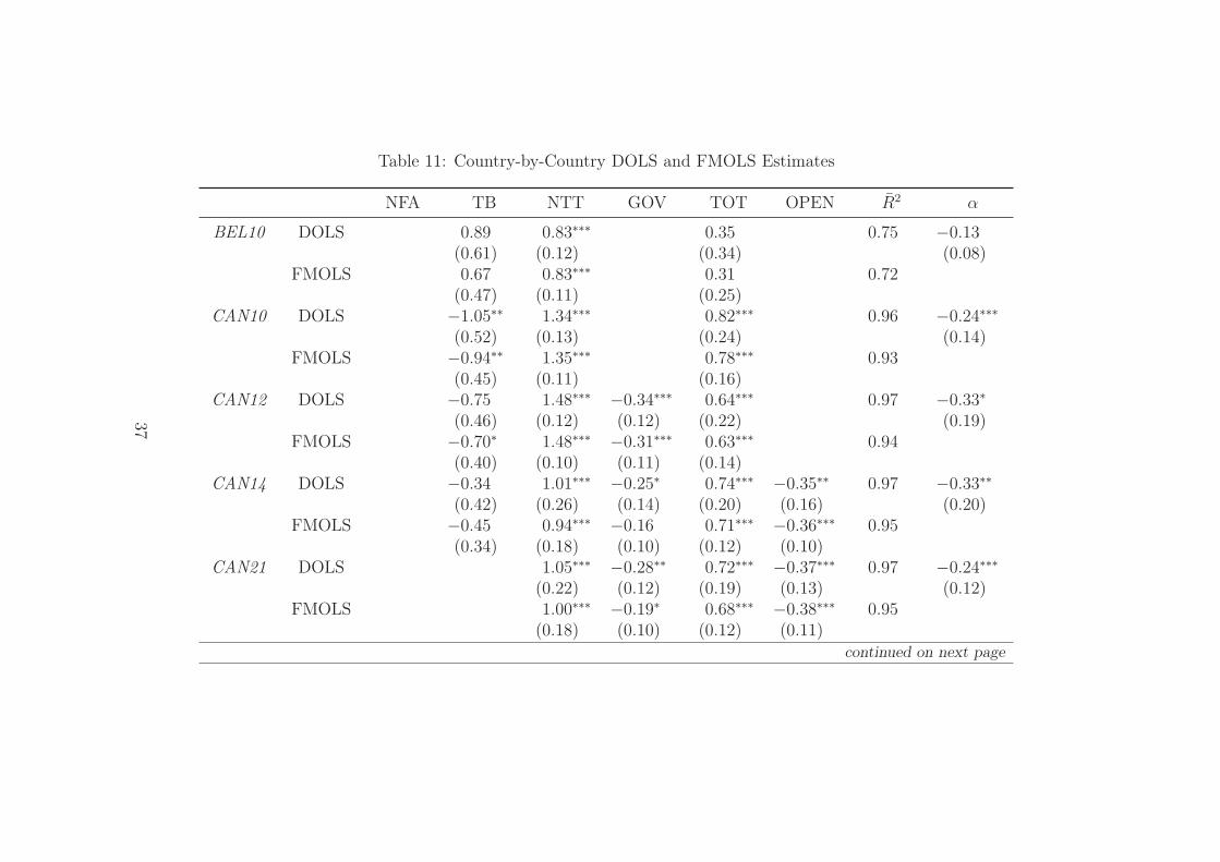
Table 11: Country-by-Country DOLS and FMOLS Estimates

NFA TB NTT GOV TOT OPEN R2 α

BEL10 DOLS 0.89 0.83∗∗∗ 0.35 0.75 −0.13(0.61) (0.12) (0.34) (0.08)

FMOLS 0.67 0.83∗∗∗ 0.31 0.72(0.47) (0.11) (0.25)

CAN10 DOLS −1.05∗∗ 1.34∗∗∗ 0.82∗∗∗ 0.96 −0.24∗∗∗

(0.52) (0.13) (0.24) (0.14)FMOLS −0.94∗∗ 1.35∗∗∗ 0.78∗∗∗ 0.93

(0.45) (0.11) (0.16)CAN12 DOLS −0.75 1.48∗∗∗ −0.34∗∗∗ 0.64∗∗∗ 0.97 −0.33∗

(0.46) (0.12) (0.12) (0.22) (0.19)FMOLS −0.70∗ 1.48∗∗∗ −0.31∗∗∗ 0.63∗∗∗ 0.94

(0.40) (0.10) (0.11) (0.14)CAN14 DOLS −0.34 1.01∗∗∗ −0.25∗ 0.74∗∗∗ −0.35∗∗ 0.97 −0.33∗∗

(0.42) (0.26) (0.14) (0.20) (0.16) (0.20)FMOLS −0.45 0.94∗∗∗ −0.16 0.71∗∗∗ −0.36∗∗∗ 0.95

(0.34) (0.18) (0.10) (0.12) (0.10)CAN21 DOLS 1.05∗∗∗ −0.28∗∗ 0.72∗∗∗ −0.37∗∗∗ 0.97 −0.24∗∗∗

(0.22) (0.12) (0.19) (0.13) (0.12)FMOLS 1.00∗∗∗ −0.19∗ 0.68∗∗∗ −0.38∗∗∗ 0.95

(0.18) (0.10) (0.12) (0.11)continued on next page

37

NFA TB NTT GOV TOT OPEN R2 α

CHN2 DOLS −0.76∗∗∗ 1.85∗∗∗ −0.67∗∗∗ 0.79 −0.37∗∗

(0.27) (0.24) (0.12) (0.12)FMOLS −0.38∗ 1.63∗∗∗ −0.49∗∗∗ 0.66

(0.21) (0.23) (0.09)CHN5 DOLS −0.75∗∗∗ 2.37∗∗∗ −0.52∗∗∗ 0.87∗∗∗ 0.91 −0.37∗∗∗

(0.16) (0.17) (0.08) (0.18) (0.15)FMOLS −0.31∗ 1.97∗∗∗ −0.37∗∗∗ 0.64∗∗∗ 0.70

(0.17) (0.21) (0.08) (0.18)CHN6 DOLS −0.47 1.63∗∗∗ −0.55∗∗∗ 0.00 0.83 −0.47∗∗∗

(0.30) (0.36) (0.18) (0.36) (0.17)FMOLS −0.53∗∗ 1.21∗∗∗ −0.33∗∗∗ −0.50∗ 0.73

(0.25) (0.30) (0.12) (0.29)CHN8 DOLS 0.95 1.71∗∗∗ 0.54 −0.20∗∗

(0.94) (0.42) (0.08)FMOLS 0.64 1.61∗∗∗ 0.47

(0.85) (0.40)CHN9 DOLS −0.92 1.12∗∗∗ −0.43∗∗∗ 0.75 −0.25∗

(0.72) (0.30) (0.09) (0.15)FMOLS −1.17∗ 1.04∗∗∗ −0.43∗∗∗ 0.70

(0.61) (0.27) (0.09)CHN10 DOLS 0.15 2.45∗∗∗ 1.39∗∗∗ 0.81 −0.24∗

(0.56) (0.25) (0.23) (0.14)continued on next page

38

NFA TB NTT GOV TOT OPEN R2 α

FMOLS 0.07 2.20∗∗∗ 1.13∗∗∗ 0.62(0.58) (0.28) (0.21)

CHN12 DOLS −0.54 1.90∗∗∗ −0.24∗∗∗ 0.95∗∗∗ 0.84 −0.33∗

(0.55) (0.29) (0.08) (0.25) (0.20)FMOLS −0.98∗∗ 1.56∗∗∗ −0.29∗∗∗ 0.68∗∗∗ 0.76

(0.48) (0.24) (0.08) (0.17)CHN14 DOLS −0.90 1.64∗∗∗ −0.28∗ 0.82∗∗∗ 0.00 0.88 −0.33∗

(0.64) (0.41) (0.14) (0.27) (0.28) (0.20)FMOLS −1.17∗∗ 1.27∗∗∗ −0.26∗∗ 0.66∗∗∗ −0.17 0.77

(0.53) (0.27) (0.12) (0.17) (0.22)CHN15 DOLS 1.39∗∗∗ 0.51 −0.18∗∗∗

(0.31) (0.06)FMOLS 1.38∗∗∗ 0.49

(0.29)CHN16 DOLS 1.42∗∗∗ −0.36∗∗∗ 0.70 −0.28∗∗

(0.21) (0.09) (0.14)FMOLS 1.41∗∗∗ 0.36∗∗∗ 0.66

(0.20) (0.08)CHN20 DOLS 1.36∗∗∗ −0.34∗∗ −0.03 0.76 −0.30∗

(0.42) (0.16) (0.38) (0.15)FMOLS 1.19∗∗∗ −0.28∗∗ −0.20 0.68

(0.33) (0.13) (0.27)GER18 DOLS 1.04∗∗∗ −0.95∗∗∗ 0.85 −0.06

continued on next page

39

NFA TB NTT GOV TOT OPEN R2 α

(0.33) (0.13) (0.08)FMOLS 0.93∗∗∗ −0.95∗∗∗ 0.83

(0.23) (0.08)GER20 DOLS 1.09∗∗∗ −0.13 −0.96∗∗∗ 0.84 −0.05

(0.36) (0.29) (0.13) (0.09)FMOLS 0.98∗∗∗ −0.16 −0.97∗∗∗ 0.83

(0.24) (0.23) (0.10)IRL5 DOLS −0.11∗∗∗ 1.77∗∗∗ −0.19∗∗ −0.17 0.89 −0.30∗∗∗

(0.03) (0.33) (0.08) (0.14) (0.11)FMOLS −0.09∗∗∗ 1.80∗∗∗ −0.19∗∗∗ −0.08 0.80

(0.02) (0.27) (0.06) (0.12)ITA11 DOLS −2.44 −1.00 −1.70∗∗∗ 0.86 −0.03

(0.68) (1.37) (0.55) (0.08)FMOLS −2.49 −0.91 −1.63∗∗∗ 0.82

(0.52) (0.96) (0.40)JPN6 DOLS −1.12∗∗∗ 1.58∗∗ 1.12∗∗∗ −6.23∗∗∗ 0.92 −0.39∗∗∗

(0.22) (0.62) (0.20) (0.67) (0.14)FMOLS −1.26∗∗∗ 1.72∗∗∗ 1.13∗∗∗ −5.58∗∗∗ 0.89

(0.19) (0.49) (0.17) (0.55)JPN7 DOLS −1.04∗∗∗ 1.64∗∗ 1.03∗∗∗ 0.10 −5.92∗∗∗ 0.92 −0.38∗∗∗

(0.21) (0.62) (0.19) (0.29) (0.99) (0.13)FMOLS −1.21∗∗∗ 1.78∗∗∗ 1.08∗∗∗ −0.00 −5.70∗∗∗ 0.89

(0.18) (0.47) (0.17) (0.17) (0.71)continued on next page

40

NFA TB NTT GOV TOT OPEN R2 α

JPN20 DOLS 2.19∗ 0.28 −6.43∗∗∗ 0.76 −0.22∗

(1.12) (0.26) (1.08) (0.11)FMOLS 1.88∗∗ 0.31 −6.32∗∗∗ 0.73

(0.79) (0.20) (8.84)KOR18 DOLS 0.11 −1.39∗∗∗ 0.76 −0.05

(0.23) (0.21) (0.08)FMOLS 0.04 −1.46∗∗∗ 0.67

(0.23) (0.20)NLD4 DOLS −0.20∗∗∗ 0.65∗∗∗ −0.57∗∗∗ 0.63 −0.20∗∗∗

(0.05) (0.21) (0.10) (0.06)FMOLS −0.19∗∗∗ 0.62∗∗∗ −0.54∗∗∗ 0.59

(0.04) (0.18) (0.08)SWE17 DOLS 0.87∗∗∗ 1.38∗∗∗ 0.93 −0.06

(0.13) (0.23) (0.45)FMOLS 0.87∗∗∗ 1.42∗∗∗ 0.87

(0.13) (0.22)US1 DOLS 0.05 2.68∗∗∗ 0.70 −0.17∗∗∗

(0.21) (0.55) (0.04)FMOLS 0.03 2.70∗∗∗ 0.64

(0.19) (0.52)US8 DOLS −6.78 0.25 0.83 −0.29∗∗∗

(1.37) (0.63) (0.08)FMOLS −5.67 0.83∗∗ 0.78

continued on next page

41

NFA TB NTT GOV TOT OPEN R2 α

(1.00) (0.41)US9 DOLS −5.60 0.90 0.19 0.85 −0.22∗∗

(1.46) (0.66) (0.12) (0.11)FMOLS −4.80 1.22∗∗∗ 0.15 0.80

(0.91) (0.42) (0.11)US15 DOLS 2.78∗∗∗ 0.67 −0.13∗∗

(0.42) (0.06)FMOLS 2.76∗∗∗ 0.65

(0.39)US16 DOLS 2.88∗∗∗ 0.25 0.77 −0.09

(0.45) (0.15) (0.07)FMOLS 2.85∗∗∗ 0.23 0.66

(0.40) (0.15)

Note: Reported are only specifications, which fulfill the following three conditions: First, all series included in the speci-fication are tested to be I(1) in the individual country’s unit root tests, secondly, the null hypothesis of no cointegrationis rejected at the 5% level according to MacKinnon critical values, and third, reer adjusts to deviations from long-runequilibrium. ***,** and * denote the significance levels of 1, 5, and 10%. α denotes the estimated adjustment parameterin the error correction form of the model.

42

92

96

100

104

108

112

116

120

124

128

132

86 88 90 92 94 96 98 00 02 04 06

AUS_REER AUS_BEER

-20

-16

-12

-8

-4

0

4

8

12

16

86 88 90 92 94 96 98 00 02 04 06

Overvaluation in %

(a) AUS

96

100

104

108

112

116

120

86 88 90 92 94 96 98 00 02 04 06

BEL_REER BEL_BEER

-8

-6

-4

-2

0

2

4

6

8

86 88 90 92 94 96 98 00 02 04 06

Overvaluation in %

(b) BEL

90

100

110

120

130

140

86 88 90 92 94 96 98 00 02 04 06

CAN_REER CAN_BEER

-12

-8

-4

0

4

8

12

86 88 90 92 94 96 98 00 02 04 06

Overvaluation in %

(c) CAN

Figure 2: REER vs. BEER and Overvaluation in Percent

43

60

70

80

90

100

110

120

130

140

150

86 88 90 92 94 96 98 00 02 04 06

CHN_REER CHN_BEER

-30

-20

-10

0

10

20

30

86 88 90 92 94 96 98 00 02 04 06

Overvaluation in %

(d) CHN

95

100

105

110

115

120

125

130

86 88 90 92 94 96 98 00 02 04 06

ESP_REER ESP_BEER

-10

-5

0

5

10

15

20

86 88 90 92 94 96 98 00 02 04 06

Overvaluation in %

(e) ESP

96

100

104

108

112

116

120

86 88 90 92 94 96 98 00 02 04 06

FRA_REER FRA_BEER

-12

-8

-4

0

4

8

12

86 88 90 92 94 96 98 00 02 04 06

Overvaluation in %

(f) FRA

Figure 2: REER vs. BEER and Overvaluation in Percent, contd.

44

96

100

104

108

112

116

120

124

128

86 88 90 92 94 96 98 00 02 04 06

GER_REER GER_BEER

-15

-10

-5

0

5

10

15

86 88 90 92 94 96 98 00 02 04 06

Overvaluation in %

(g) GER

95

100

105

110

115

120

125

130

135

86 88 90 92 94 96 98 00 02 04 06

IRL_REER IRL_BEER

-10.0

-7.5

-5.0

-2.5

0.0

2.5

5.0

7.5

10.0

86 88 90 92 94 96 98 00 02 04 06

Overvaluation in %

(h) IRL

90

95

100

105

110

115

120

125

130

86 88 90 92 94 96 98 00 02 04 06

ITA_REER ITA_BEER

-20

-15

-10

-5

0

5

10

15

86 88 90 92 94 96 98 00 02 04 06

Overvaluation in %

(i) ITA

Figure 2: REER vs. BEER and Overvaluation in Percent, contd.

45

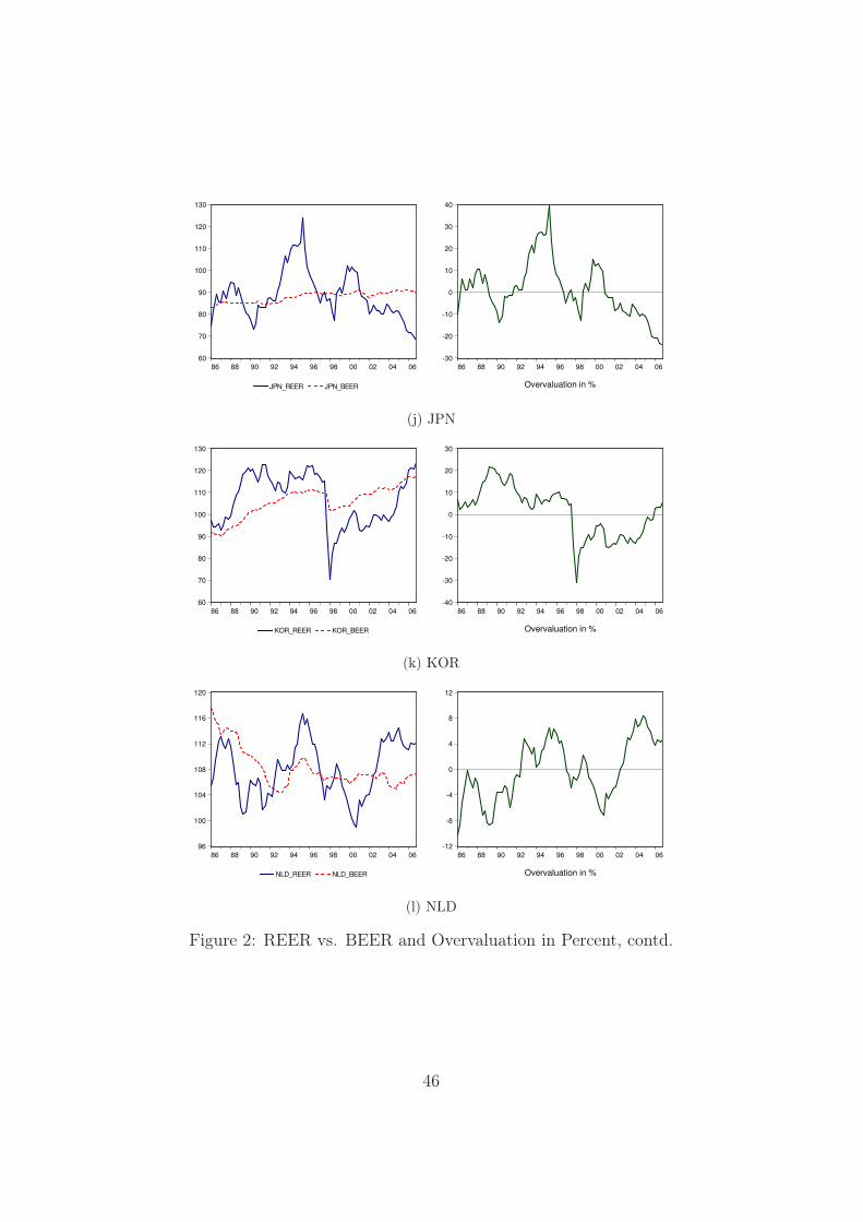
60

70

80

90

100

110

120

130

86 88 90 92 94 96 98 00 02 04 06

JPN_REER JPN_BEER

-30

-20

-10

0

10

20

30

40

86 88 90 92 94 96 98 00 02 04 06

Overvaluation in %

(j) JPN

60

70

80

90

100

110

120

130

86 88 90 92 94 96 98 00 02 04 06

KOR_REER KOR_BEER

-40

-30

-20

-10

0

10

20

30

86 88 90 92 94 96 98 00 02 04 06

Overvaluation in %

(k) KOR

96

100

104

108

112

116

120

86 88 90 92 94 96 98 00 02 04 06

NLD_REER NLD_BEER

-12

-8

-4

0

4

8

12

86 88 90 92 94 96 98 00 02 04 06

Overvaluation in %

(l) NLD

Figure 2: REER vs. BEER and Overvaluation in Percent, contd.

46

80

90

100

110

120

130

140

86 88 90 92 94 96 98 00 02 04 06

SWE_REER SWE_BEER

-15

-10

-5

0

5

10

15

86 88 90 92 94 96 98 00 02 04 06

Overvaluation in %

(m) SWE

70

75

80

85

90

95

100

105

110

86 88 90 92 94 96 98 00 02 04 06

UK_REER UK_BEER

-20

-16

-12

-8

-4

0

4

8

12

16

86 88 90 92 94 96 98 00 02 04 06

Overvaluation in %

(n) UK

80

84

88

92

96

100

104

108

86 88 90 92 94 96 98 00 02 04 06

US_REER US_BEER

-15

-10

-5

0

5

10

15

86 88 90 92 94 96 98 00 02 04 06

Overvaluation in %

(o) US

Figure 2: REER vs. BEER and Overvaluation in Percent, contd.

47