The Harrod-Balassa-Samuelson Hypothesis: Real Exchange ... · The Harrod-Balassa-Samuelson...

NBER WORKING PAPER SERIES

THE HARROD-BALASSA-SAMUELSON HYPOTHESIS:REAL EXCHANGE RATES AND THEIR LONG-RUN EQUILIBRIUM

Yanping ChongÒscar Jordà

Alan M. Taylor

Working Paper 15868http://www.nber.org/papers/w15868

NATIONAL BUREAU OF ECONOMIC RESEARCH1050 Massachusetts Avenue

Cambridge, MA 02138April 2010

Jordà is grateful for the support from the Spanish MICINN National Grant SEJ2007-6309 and thehospitality of the Federal Reserve Bank of San Francisco during preparation of this manuscript. Tayloralso gratefully acknowledges research support from the Center for the Evolution of the Global Economyat the University of California, Davis. The views expressed herein are those of the authors and do notnecessarily reflect the views of the National Bureau of Economic Research.

NBER working papers are circulated for discussion and comment purposes. They have not been peer-reviewed or been subject to the review by the NBER Board of Directors that accompanies officialNBER publications.

© 2010 by Yanping Chong, Òscar Jordà, and Alan M. Taylor. All rights reserved. Short sections oftext, not to exceed two paragraphs, may be quoted without explicit permission provided that full credit,including © notice, is given to the source.

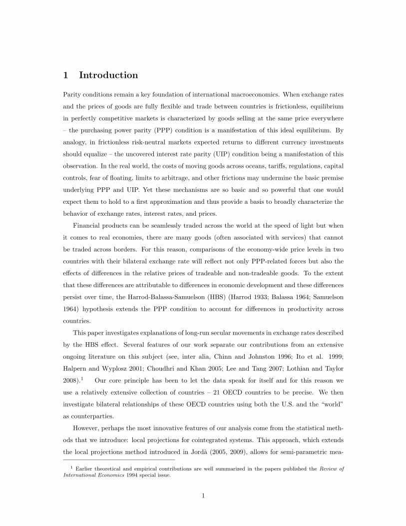
The Harrod-Balassa-Samuelson Hypothesis: Real Exchange Rates and their Long-Run EquilibriumYanping Chong, Òscar Jordà, and Alan M. TaylorNBER Working Paper No. 15868April 2010JEL No. F31,F41

ABSTRACT

Frictionless, perfectly competitive traded-goods markets justify thinking of purchasing power parity(PPP) as the main driver of exchange rates in the long-run. But differences in the traded/non-tradedsectors of economies tend to be persistent and affect movements in local price levels in ways that upsetthe PPP balance (the underpinning of the Harrod-Balassa-Samuelson hypothesis, HBS). This paperuses panel-data techniques on a broad collection of countries to investigate the long-run propertiesof the PPP/HBS equilibrium using novel local projection methods for cointegrated systems. Thesesemi-parametric methods isolate the long-run behavior of the data from contaminating factors suchas frictions not explicitly modelled and thought to have effects only in the short-run. Absent the short-runeffects, we find that the estimated speed of reversion to long-run equilibrium is much higher. In addition,the HBS effects means that the real exchange rate is converging not to a steady mean, but to a slowlyto a moving target. The common failure to properly model this effect also biases the estimated speedof reversion downwards. Thus, the so-called "PPP puzzle" is not as bad as we thought.

Yanping ChongUC, [email protected]

Òscar JordàDept. of EconomicsUC, DavisOne Shields Ave.Davis, CA [email protected]

Alan M. TaylorDepartment of EconomicsUniversity of California, DavisOne Shields AvenueDavis, CA 95616and [email protected]

1 Introduction

Parity conditions remain a key foundation of international macroeconomics. When exchange rates

and the prices of goods are fully flexible and trade between countries is frictionless, equilibrium

in perfectly competitive markets is characterized by goods selling at the same price everywhere

– the purchasing power parity (PPP) condition is a manifestation of this ideal equilibrium. By

analogy, in frictionless risk-neutral markets expected returns to different currency investments

should equalize – the uncovered interest rate parity (UIP) condition being a manifestation of this

observation. In the real world, the costs of moving goods across oceans, tariffs, regulations, capital

controls, fear of floating, limits to arbitrage, and other frictions may undermine the basic premise

underlying PPP and UIP. Yet these mechanisms are so basic and so powerful that one would

expect them to hold to a first approximation and thus provide a basis to broadly characterize the

behavior of exchange rates, interest rates, and prices.

Financial products can be seamlessly traded across the world at the speed of light but when

it comes to real economies, there are many goods (often associated with services) that cannot

be traded across borders. For this reason, comparisons of the economy-wide price levels in two

countries with their bilateral exchange rate will reflect not only PPP-related forces but also the

effects of differences in the relative prices of tradeable and non-tradeable goods. To the extent

that these differences are attributable to differences in economic development and these differences

persist over time, the Harrod-Balassa-Samuelson (HBS) (Harrod 1933; Balassa 1964; Samuelson

1964) hypothesis extends the PPP condition to account for differences in productivity across

countries.

This paper investigates explanations of long-run secular movements in exchange rates described

by the HBS effect. Several features of our work separate our contributions from an extensive

ongoing literature on this subject (see, inter alia, Chinn and Johnston 1996; Ito et al. 1999;

Halpern and Wyplosz 2001; Choudhri and Khan 2005; Lee and Tang 2007; Lothian and Taylor

2008).1 Our core principle has been to let the data speak for itself and for this reason we

use a relatively extensive collection of countries – 21 OECD countries to be precise. We then

investigate bilateral relationships of these OECD countries using both the U.S. and the “world”

as counterparties.

However, perhaps the most innovative features of our analysis come from the statistical meth-

ods that we introduce: local projections for cointegrated systems. This approach, which extends

the local projections method introduced in Jorda (2005, 2009), allows for semi-parametric mea-

1 Earlier theoretical and empirical contributions are well summarized in the papers published the Review ofInternational Economics 1994 special issue.

1

surement of the dynamics of long-run equilibrium adjustment. Moreover, local projections provide

a natural and simple separation of these adjustment dynamics into the component explained purely

by long-run forces (encapsulated primarily in the HBS hypothesis) from the component explained

by frictions thought to have effects only in the short-run and for which no explicit economic justi-

fication is given nor sought in this paper. We hope that discerning readers will find the methods

useful for applications other than the one offered in this paper.

Traditionally, cointegration is examined through the prism of a vector error-correction model

(VECM) but VECMs are difficult to extend to panels because they are parametrically intensive.

In addition, parametrically tractable specifications and the structure of VECMs restrict the range

of dynamics and half-lives that can be estimated from the data. Finally, conventional estimates

from these models offer half-live estimates that conflate the process of long-run adjustment (the

focus of this paper) with the effect of short-run frictions on long-run adjustment (not the focus of

this paper). To be sure, we are not advocating that forces other than those encapsulated by the

HBS effect are unimportant in explaining exchange rate movements. Much like a feather blown

by the wind returns to the ground by the force of gravity, so do exchange rates return to their

long-run equilibrium levels and the strength of this pull is the object of our interest. But just as

the flight of the feather follows the whimsy of the wind, so do exchange rates follow the whimsy

of forces whose characterization we reserve for future research.

2 Statistical Design

2.1 Preliminaries

We begin by presenting the basic set-up in a more traditional linear context to better communicate

the main ideas. Let et+1 denote the logarithm of the nominal exchange rate in terms of currency

units of domestic currency per units of foreign currency, let pt+1 and p∗t+1 denote the logarithm

of the price indices home and abroad. In the strict version of PPP without frictions and where

the price indices refer only to traded goods, then the real exchange rate defined as qt+1 = et+1 +

(p∗t+1−pt+1) would only exhibit temporary fluctuations around a long-run equilibrium level, or in

time series parlance, it would be a stationary variable and hence implicitly define a cointegrating

vector. Similarly, let it and i∗t denote the one-period, risk-free interest rate home and abroad.

The UIP condition can be seen as a statement about the absence of arbitrage of a zero net

investment position. Specifically, let the variable momentum denoted as mt refer to the ex-ante

nominal excess returns of such an investment, i.e., mt+1 = (i∗t − it) + ∆et+1, then in the absence

of arbitrage opportunities the ex-ante value of momentum should be zero, that is Etmt+1 = (i∗t −

it) +Et∆et+1 = 0, which should make mt+1 a stationary and unpredictable variable. Momentum

2

can also be expressed in terms of real excess returns as

mt+1 = (r∗t − rt) + ∆qt+1 (1)

where rt = it − πt+1 with πt+1 = ∆pt+1, and similarly for r∗t and π∗t+1; and qt+1 = et+1 +

(p∗t+1− pt+1) so that ∆qt+1 = ∆et+1 +(π∗t+1 − πt+1

). This reformulation of momentum with real

variables makes the interaction between PPP and UIP more readily apparent. Finally, we extend

the formulation of the system with xt+1 and x∗t+1, which denote the logarithm of home and abroad

productivity proxies. If qt+1 is not a stationary variable, persistent deviations from long-run

equilibrium could be explained by persistent productivity differentials (in the traded/non-traded

composition) between trading partners according to the Harrod-Balassa-Samuelson hypothesis.

The implication of this hypothesis can be stated in terms of the variable zt+1 = qt+1 − β(x∗t+1 −

xt+1), which should be stationary under the HBS hypothesis.

The dynamic interactions between nominal exchange rates, inflation, interest rate and produc-

tivity differentials are the constituent elements of a system whose linear combinations explain the

dynamic behavior of HBS-adjusted PPP, and UIP jointly, specifically

∆yt+1 =

∆et+1

π∗t+1 − πt+1

i∗t − it∆x∗t+1 −∆xt+1

. (2)

Several features of this system deserve mention. We will show momentarily that et+1, (p∗t+1 −

pt+1), and (x∗t+1 − xt+1) are I(1) variables but that they are cointegrated (and hence ∆yt+1 is

I(0)), a property that we exploit to derive the HBS-adjusted PPP relation below. In addition,

we will show formally (in Table 1 below) that each of the elements in ∆yt+1 is stationary with

appropriate panel unit root tests. The timing of the variable (i∗t − it) may seem odd but simply

reflects the observation that at time t, the interest rate for delivery at time t+1 is known. Finally,

appropriate panel cointegration tests reported in Table 2 show that zt+1 = qt+1 − β(x∗t+1 − xt+1)

is a proper cointegration vector.

Notice that expression (2) does not characterize the stochastic process we think ∆yt+1 may

follow. This is by design since we will be interested in calculating certain sample statistics of

interest without referencing to any one specific model. The tools required to estimate these

sample statistics are discussed in the next section.

3

2.2 Local Projections for Cointegrated Systems

Long-run equilibrium in exchange rates under the HBS hypothesis takes on the form zt+1 =

et+1 + (p∗t+1 − pt+1) − β(x∗t+1 − xt+1). When β = 0 this is clearly just the usual PPP condition.

We are interested in learning how long-run equilibrium is restored in response to shocks and how

this adjustment process manifests itself in the dynamics of nominal exchange rates and prices.

In order to present our approach, we find it convenient to discuss the basic features of a typical

linear specification first. We do this with as general a notation as possible to accommodate

applications other than the one we pursue in this paper for the benefit of readers with other

applications in mind. Suppose yt is an n × 1 vector of non-stationary random variables, such as

that in expression (2), that is first-difference stationary with Wold representation:

∆yt =∞∑j=0

Cjεt−j (3)

where the constant and other deterministic components are omitted for convenience but without

loss of generality. The n × n matrices Cj are such that C0 = In;∑∞j=0 j||Cj || < ∞ where

||Cj ||2 = tr(C ′jCj); and εt is an n×1 vector white noise (relaxing these and subsequent assumptions

is certainly possible but distracting from the exposition of the main results here).

Further, assume that yt has a finite vector autoregressive (VAR) representation of order p+ 1

in the levels and given by

yt+1 = Φ1yt + ...+ Φp+1yt−p + εt+1 (4)

where the Φj j = 1, ..., p + 1 are n × n coefficient matrices. Expression (4) can be equivalently

written (see e.g. Hamilton, 1994) as

yt+1 = Ψ1∆yt + ...+ Ψp∆yt−p+1 + Πyt + εt+1 (5)

with Ψj = − [Φj+1 + ...+ Φp+1] , j = 1, ..., p and Π =∑p+1j=1 Φj . Subtracting yt from both sides

of expression (5) we obtain

∆yt+1 = Ψ1∆yt + ...+ Ψp∆yt−p+1 + Ψ0yt + εt+1 (6)

where Ψ0 = Π− I = −Φ(1).

When there is cointegration among the elements of yt, then there exists an n × k matrix A

such that zt = A′yt is I(0) and contains the k cointegrating vectors. In our specific application

k = 1. Further, the n× n matrix Φ(1) is reduced-rank with rank k and thus can be expressed as

Φ(1) = BA′ where B is an n × k matrix so that expression (6) becomes the well-known error-

correction representation for yt. Notice that (3) can be recast as

yt = y0 + C(1)t∑

j=1

εj +∞∑j=0

C∗j εt−j −∞∑j=0

C∗j ε−j

4

and assuming for convenience that the initial conditions y0 and ε−j are zero, further simplified

into

yt = C(1)t∑

j=1

εj +∞∑j=0

C∗j εt−j (7)

where the first term contains the stochastic trend components, the second term the cyclical com-

ponents and C∗j = − [Cj+1 + ...] , j = 0, 1, ... Expression (7) is the well-known Beveridge-Nelson

decomposition and when there is cointegration, A′yt is stationary which implies that A′C(1) = 0

and hence an impulse response representation for zt can be easily derived to be from (7)

zt =∞∑j=0

A′C∗j εt−j = A′∞∑j=0

(j∑i=0

Ciεt−j

). (8)

This is the essence of the Granger-representation theorem.

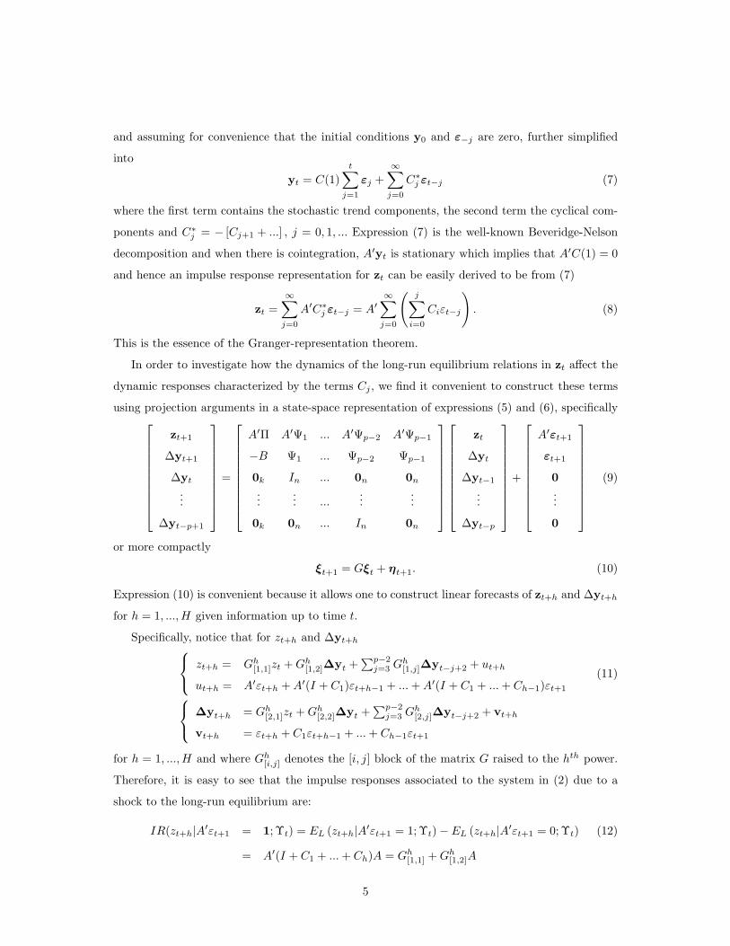
In order to investigate how the dynamics of the long-run equilibrium relations in zt affect the

dynamic responses characterized by the terms Cj , we find it convenient to construct these terms

using projection arguments in a state-space representation of expressions (5) and (6), specifically

zt+1

∆yt+1

∆yt...

∆yt−p+1

=

A′Π A′Ψ1 ... A′Ψp−2 A′Ψp−1

−B Ψ1 ... Ψp−2 Ψp−1

0k In ... 0n 0n...

... ......

...

0k 0n ... In 0n

zt

∆yt

∆yt−1

...

∆yt−p

+

A′εt+1

εt+1

0...

0

(9)

or more compactly

ξt+1 = Gξt + ηt+1. (10)

Expression (10) is convenient because it allows one to construct linear forecasts of zt+h and ∆yt+h

for h = 1, ...,H given information up to time t.

Specifically, notice that for zt+h and ∆yt+h zt+h = Gh[1,1]zt +Gh[1,2]∆yt +∑p−2j=3 G

h[1,j]∆yt−j+2 + ut+h

ut+h = A′εt+h +A′(I + C1)εt+h−1 + ...+A′(I + C1 + ...+ Ch−1)εt+1

(11)

∆yt+h = Gh[2,1]zt +Gh[2,2]∆yt +∑p−2j=3 G

h[2,j]∆yt−j+2 + vt+h

vt+h = εt+h + C1εt+h−1 + ...+ Ch−1εt+1

for h = 1, ...,H and where Gh[i,j] denotes the [i, j] block of the matrix G raised to the hth power.

Therefore, it is easy to see that the impulse responses associated to the system in (2) due to a

shock to the long-run equilibrium are:

IR(zt+h|A′εt+1 = 1; Υt) = EL (zt+h|A′εt+1 = 1; Υt)− EL (zt+h|A′εt+1 = 0; Υt) (12)

= A′(I + C1 + ...+ Ch)A = Gh[1,1] +Gh[1,2]A

5

and

IR(∆yt+h|A′εt+1 = 1; Υt) = EL(∆yt+h|A′εt+1 = 1; Υt

)− EL

(∆yt+h|A′εt+1 = 0; Υt

)(13)

= ChA = Gh[2,1] +Gh[2,2]A

Several features of expressions (12) and (13) deserve comment. First, the definitions of the im-

pulse responses are somewhat unusual because they have the flavor of a dynamic average treatment

effect where the treatment is standardized to be A′εt+1 = 1 and the non-treatment A′εt+1 = 0.

That is, the impulse response focuses directly on disturbances to long-run equilibrium, but it

is not explicit about the source of this disturbance (i.e. we do not examine shocks to any one

particular element of ∆yt+1). In our application A is n× 1 so that zt+1 is scalar and A′εt+1 = 1

is also scalar and uniquely determined. For this reason, we are not required to make the type

of identification assumption (such as the ubiquitous Cholesky assumptions) commonly found in

the vector autoregressive (VAR) literature regarding the constituent elements in ∆yt+1. Second,

for reference to what has been traditional in the literature in the past we note that the usual

(not-orthogonalized) impulse responses analyzed correspond to the elements in Ch in expression

(13), which in our set up amounts to Gh[2,1]A′+Gh[2,2]. Third, notice that the impulse responses in

expressions (12) and (13) depend on the sum of two components, Gh[i,1] and Gh[i,2], i ∈ 1, 2. The

terms Gh[i,1] describe the effect that adjustment to the long-run equilibrium zt has on the impulse

response. The terms Gh[i,2] describe instead the effect that the short-run dynamics in ∆yt+1 have

on the impulse response. In our application, such demarcation is very useful because it orthogo-

nalizes the dynamic response to the PPP-HBS term from the response to short-term frictions due

to unmodelled factors.

It has been traditional to estimate vector error correction models (VECMs) and obtain esti-

mates of the system’s impulse responses (Ch) with nonlinear transformations of the conditional

mean parameter estimates. Instead, we find it more convenient and suitable to the economic

question of interest to directly estimate the terms Gh[i,j] i, j ∈ 1, 2 with local projections (Jorda

2005, 2009) from expressions (11). This is advantageous for several reasons: (1) direct estimates

of expressions (11) can be done equation by equation with little loss of efficiency (see Jorda, 2005)

and therefore can be adapted directly to panel estimation. A VECM specification is too para-

metrically intensive in our application to afford sufficiently rich dynamics; (2) direct estimation

of (11) does not restrict the dynamics of the estimated impulse responses across periods and is

therefore robust to misspecification and generalizable to allow for nonlinear effects (see Jorda 2005

for examples in the stationary context); (3) because the coefficients in Gh[i′j] i, j ∈ 1, 2 are com-

puted directly from regression, computation of standard errors is straight-forward. By contrast,

6

VECM estimates are based on nonlinear functions of estimated parameters with differing rates

of asymptotic convergence which complicates calculation of appropriate inferential procedures;

and (4) direct estimates provide the orthogonalization of the impulse responses that we seek in a

natural and uncomplicated way whereas orthogonalization with VECM estimates would require

complicated nonlinear transformations once again.

To get a better sense of the large sample properties of the local projection estimator, consider

first the simpler non-panel case. Let ZH be the (T − p−H)×kH matrix that collects observations

for (zt+1, ..., zt+H)′ ; and let YH be the (T − p−H) × nH matrix that collects observations for

(∆yt+1, ...,∆yt+H)′ . Next define the regressor matrices, with X a (T − p−H)× (k + n) matrix

that collects observations for (zt,∆yt)′ and W a (T − p−H) × (1 + np) matrix that collects

observations for (1,∆yt−1, ...,∆yt−p)′. Notice that W collects all the regressors whose coefficients

are of no direct interest and hence the matrix M = I −W (W ′W )−1W ′ projects their effect away.

A direct estimate of the Gh[i,j] given a first stage estimate of A′ by conventional methods (or

based on economic restrictions) can be found easily with the local projection estimator

Gz(k+n)×kH

=

G1[1,1] ... GH[1,1]

G1[1,2] ... GH[1,2]

= (X ′MX)−1 (X ′MZH) (14)

Gy(k+n)×nH

=

G1[2,1] ... GH[2,1]

G1[2,2] ... GH[2,2]

= (X ′MX)−1 (X ′MYH)

with covariance matrices for gz = vec(GZ) and gy = vec(Gy) respectively

Ωi =[(X ′MX)−1 ⊗ Σi

]; Σi =

V ′i ViT − p−H

for i ∈ z, y (15)

with Vz = MZH −MXGz and Vy = MYH −MXGy. Thus, the impulse responses in expression

(13) can be constructed given estimates A, Gz and Gy. Further, since A′ is either imposed from

theory or superconsistently estimated from typical cointegration procedures, then the standard

regularity conditions made in expression (3) and the results in proposition 2 in Jorda and Kozicki

(2010) are all that is needed to show that√T − p−H (gi − gi)→ N (0,Ωi) ; i ∈ z, y

so that standard inferential procedures are readily available using (14) and (15).

A convenient feature of the local projection approach discussed in Jorda (2005) is that to

estimate impulse responses in practice, one can obtain consistent estimates of the elements of

Gh[i,j] using equation-by-equation methods with little loss of efficiency when standard errors are

calculated with non-parametric heteroscedasticity and autocorrelation robust (HAC) variance-

covariance matrix estimators. Since most econometric packages are well suited to estimate panel

7

regressions, and have pre-built routines for (HAC) variance-covariance estimators, we find useful

to take this more convenient approach since it lowers entry barriers to other researchers wishing

to use our methods.

Extensions of the local projection estimator to panels in (11) is therefore straight-forward.

In our application, we estimate (11) equation by equation for the panel of countries we consider

and allow for country-fixed effects. It is well-known that in a regression model for panel data

containing lags of the endogenous variable, the within-groups estimator can be severely downward

biased when the serial correlation in the endogenous variable is high and the time series dimension

T is short, regardless of the cross-section dimension M. This is often called the Nickell (1981) bias

and a standard solution is to apply the Arellano and Bond (1991) GMM estimator. However, in

our setting T = 31 and M = 21 which perhaps is best characterized by T/M → c > 0, T,M →∞

asymptotics. Alvarez and Arellano (2003) show that in this case, the within-group estimator has

a vanishing downward bias. In the simple case with no exogenous regressors and first order serial

correlation, this bias is (1/T )(1 + ρ), where ρ is the autocorrelation coefficient. For example, in

the extreme where ρ ≈ 1, the bias is approximately 0.06 given our sample size. However, the

crude GMM estimator in this case is inconsistent despite being consistent for fixed T. For this

reason we proceed with the within-group estimator. We remark on these issues because readers

may find the panel-cointegration impulse response estimator useful for other applications where

the rates at which M and T grow will differ from ours and where different estimation procedures

will be indicated. The reader is referred to Alvarez and Arellano (2003), who provide a very good

discussion on these issues.

Summarizing, the half-life of the PPP/HBS relation can be estimated directly by regressing

leads of the cointegrating vector on its current values and on current and lagged values of ∆yt.

Standard errors for the relevant coefficients can be obtained by standard methods, which facilitate

construction of confidence bands. The approach has several advantages: although we use a linear

set-up to explain the method, it should be clear that ours is a semi-parametric method that does

not restrict the half-life to decay monotonically. More generally and as is discussed in Jorda (2005),

there is no obligation to rely on linear projections and one is free to examine nonlinear adjustment

to long-run equilibrium with nonlinear projections (an approach best left for another paper here).

Nonlinearities are easily accommodated with our equation-by-equation approach because they do

not require full blown specification of what the nonlinear stochastic process for the entire system

might be.

8

3 Data Description

We begin by describing the data. Our analysis is based on quarterly data over the 1973Q2–

2008Q4 period for 21 OECD countries: Australia, Austria, Belgium, Canada, Denmark, Finland,

France, Germany, Greece, Ireland, Italy, Japan, Netherlands, Norway, New Zealand, Portugal,

Spain, Sweden, Switzerland, the United Kingdom and the United States. Nominal exchange rates

and CPI data come mainly from the International Financial Statistics (IFS) database maintained

by the IMF, except for Germany’s CPI, available from the OECD’s Main Economic Indicators

database. CPI data are not seasonally adjusted at the source and therefore were harmonized with

the X11 procedure, which is the standard method of seasonal adjustment for many statistical

agencies. Data on GDP and GDP deflators (denoted PGDP) come primarily from the OECD’s

Outlook database (except for Germany, which comes from the IFS database). Interest rate data

come from the Global Financial database. A data file with full descriptions is available upon

request.2

Throughout our analysis, lowercase symbols will always denote logarithms. Bilateral compar-

isons are made with respect to a reference country (denoted with the superscript * in expression

2). The U.S. is a natural counterparty and so is the “rest of the world.” We consider the latter as

it is well known that the choice of base country can substantially affect the statistical properties

of real exchange rate dynamics. In particular, induced cross-sectional dependence can be an issue

(see, e.g. O’Connell, 1998) and bias may result from the idiosyncratic behavior of a particular

base country (see, e.g. Taylor, 2002).

In the case of the U.S. base, we construct for all other countries i the logarithms of real

exchange rates as qUSit = eUSit + pUSt − pit, where eUSit is the log nominal exchange rate, denoted

in units of home currency per USD, and pit and pUSt are the log CPI levels of the home country

and the U.S., respectively. An increase in qUSit means a real depreciation of home currency, i.e.,

home goods are becoming less expensive relative to the U.S. The relative productivity term, or

HBS term, is naıvely measured by the log real GDP per capita ratio, xUSt −xit, where xit and xUSt

denote the log real GDP per capita levels of the home country and the U.S., respectively. The

inflation differential is defined as πUSt − πit, where πit and πUSt are the inflation rates in percent

per quarter for each country, while the interest rate differential is defined as, iUSt − iit, where iit

2 Note that in the OECD databases, data for the Euro area countries are now expressed in euro, so pre-1999data were converted from national currency using official euro conversion rates. Consequently, “national currency”in always refers to euro for the Euro area countries, and not the legacy currencies. Germany GDP data from theIFS in billions of deutsche mark at quarterly level were converted to millions of Euro at annual level. Regarding3-month interest rate series, in cases that 3-month interbank rates (IB) are not available, changes of alternativerates were applied to the end IB observation to recover levels. The alternative rates we used as substitutes were(in order of preference) the 3-month commercial paper rate, the 3-month T-bill rate, Government note yields, andother fixed-income rates. For the 11 Euro area countries, the EuroLIBOR rates are spliced at the end.

9

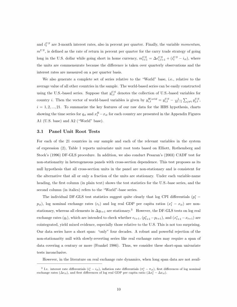
and iUSt are 3-month interest rates, also in percent per quarter. Finally, the variable momentum,

mUS , is defined as the rate of return in percent per quarter for the carry trade strategy of going

long in the U.S. dollar while going short in home currency, mUSt+1 = ∆eUSi,t+1 + (iUSt − iit), where

the units are commensurate because the difference is taken over quarterly observations and the

interest rates are measured on a per quarter basis.

We also generate a complete set of series relative to the “World” base, i.e., relative to the

average value of all other countries in the sample. The world-based series can be easily constructed

using the U.S.-based series. Suppose that yUSi,t denotes the collection of U.S.-based variables for

country i. Then the vector of world-based variables is given by yWorldi,t = yUSi,t − 1

M−1

∑j 6=i y

USj,t ,

i = 1, 2, ..., 21. To summarize the key features of our raw data for the HBS hypothesis, charts

showing the time series for qit and xRt −xit for each country are presented in the Appendix Figures

A1 (U.S. base) and A2 (“World” base).

3.1 Panel Unit Root Tests

For each of the 21 countries in our sample and each of the relevant variables in the system

of expression (2), Table 1 reports univariate unit root tests based on Elliott, Rothemberg and

Stock’s (1996) DF-GLS procedure. In addition, we also conduct Pesaran’s (2003) CADF test for

non-stationarity in heterogeneous panels with cross-section dependence. This test proposes as its

null hypothesis that all cross-section units in the panel are non-stationary and is consistent for

the alternative that all or only a fraction of the units are stationary. Under each variable-name

heading, the first column (in plain text) shows the test statistics for the U.S.-base series, and the

second column (in italics) refers to the “World”-base series.

The individual DF-GLS test statistics suggest quite clearly that log CPI differentials (p∗t −

pit), log nominal exchange rates (et) and log real GDP per capita ratios (x∗t − xit) are non-

stationary, whereas all elements in ∆yt+1 are stationary.3 However, the DF-GLS tests on log real

exchange rates (qt), which are intended to check whether et+1, (p∗t+1−pt+1), and (x∗t+1−xt+1) are

cointegrated, yield mixed evidence, especially those relative to the U.S. This is not too surprising.

Our data series have a short span: “only” four decades. A robust and powerful rejection of the

non-stationarity null with slowly-reverting series like real exchange rates may require a span of

data covering a century or more (Frankel 1986). Thus, we consider these short-span univariate

tests inconclusive.

However, in the literature on real exchange rate dynamics, when long span data are not avail-

3 I.e. interest rate differentials (i∗t − iit), inflation rate differentials (π∗t − πit), first differences of log nominalexchange rates (∆eit), and first differences of log real GDP per capita ratio (∆x∗t − ∆xit).

10

!"#$%$#&'()*+,-./

0&123'($'

,4567

!"#$

4588

!"#$%

,859:

!&#"&

,85;<

!&#&'

,85=:>>

!&#('

,656;>>

!)#(%**

,858<

!)#(+**

,85<<

!(#$&***

0&123$'

,45:=

"#'(

,4569

!"#,,

,45??

!"#'%

,85:6>

!&#(

,;568>>>

!&#,,*

,6568>>

!"#-(

,658=>>

!&#+,*

,8574>

!+#,(***

@A(B$&C

,65;?>>

"#&&

,45:

"#))

,85=7>>

!&#'+*

,6594>>

!&#%)

,957<>>>

!&#,-*

,6588>>

!&#(+

,856=

!)#&)**

,45=9

!&#&,

D'"'#'

,45==

!)#&+**

,45:

"#$)

,8569

!"#,%

,8566

!&#)$

,65;;>>

!-#&-***

,9598>>>

!)#-)**

,8576>

!-#)"***

,85;8

!-#)+***

*A"C'3E

,85=<>>

"#"&

,45;=

"#(

,4586

"#%)

,65<?>>

!)#"'**

,;5?6>>>

!-#)$***

,85:7>

!)#&'**

,6576>>>

!&#($

,85=7>>

!)#',***

+$"('"#

,85?<>

!)#)"**

,458

!"#%,

,456=

!&#)'

,65<<>>

!&#+(*

,;58;>>>

!-#-+***

,659<>>

!)#%+**

,8578>

!)#%)**

,45??

!"#'&

+3'"FA

,85;8

!&#(%

,4577

!"#&

,859;

"#&(

,6549>>

!&#&)

,65<9>>

!&#"&

,85=6>

!&#))

,659?>>

!)#),**

,856;

!-#--***

-A3C'"G

,858?

"#%&

4547

"#"-

,85?8>

!&#+)*

,85==>>

!"#,$

,;5?8>>>

!(#%$***

,65<9>>

!&#(%

,8567

!"#(+

,65:<>>>

!-#'-***

-3AAFA

456:

!"#&'

,456

!"#-,

,4579

!"#(%

,854:

!"#-&

,65?=>>>

!&#),

,8598

!&#(

,45:8

!"#$-

,85??>

!-#-&***

!3A('"#

,45=9

!"#+'

,454;

!"#)$

45=?

"#-+

,85;8

!"#)$

,859<

!"#&

,659<>>

!)#)&**

,65;?>>

!)#&&**

,8576>

!)#-%**

!2'(G

,459;

"#&(

458

!"#&%

,858

!"#--

,6597>>

!)#('**

,6568>>

!&#"%

,85?:>

!&#(+

,856?

!&#((

,459=

!"#)&

H'I'"

4"#%(

45<;

"#%,

,8566

!&#&%

,8569

!"#'$

,;5?;>>>

!(#'+***

,854;

!"#'+

,65:=>>>

!&#((

,65??>>>

!&#+"*

JA2KA3('"#1

,859;

"#%'

,4589

!"#%&

,859?

!"#()

,65<<>>

!&#++*

,657;>>>

!&#),

,658?>>

!&#&,

,85;6

!&#&%

,;5:4>>>

!"#-&

JALMNA'('"#

,459<

!"#((

456

!"#"$

,45?=

!"#)%

,65;9>>

!-#))***

,4577

!"#('

,65<6>>

!)#(%**

,658;>>

!)#%&**

,45?9

!"#%%

JO3L'G

,85;:

!&#(,

,45??

!"#"-

8568

"#&+

,656:>>

!&#,,*

,656<>>

!&#-,

,95;6>>>

!(#(%***

,65=6>>>

!&#+(*

,454=

!"#&%

PO32&B'(

454<

"458

"#"(

,8549

!&#"+

,85:6>

!&#&+

,65:;>>>

!)#%-**

,6547>>

!&#(-

,8!"#,

,85<:

!)#+"***

/I'$"

,45?

!"#&,

45;8

"#)(

,4577

!"#-&

,859<

!"#%(

,65;=>>

!&#',*

,85:9>

!&#'$*

,85<7

!)#,%***

,854;

!&#(&

/LA#A"

,4578

!"#&)

,4596

!"#))

,85<7

!"#,'

,85;<

"#%)

,65<:>>

!&#$-*

,9589>>>

!-#"-***

,85?;>

!&#&

,85<=

!-#+,***

/L$2QA3('"#

,454<

"#+(

,454?

!"#-

45?<

&#%

,85<<

!&#&&

,;589>>>

!)#"$**

,85?:>

!&#%'

,85;=

!)#"&**

,85<8

!)#-%**

R"$2A#MS$"B#

,4577

!&#))

45:;

"#))

,8589

!&#&$

,6547>>

!&#+,*

,85<6

!&#&

,6547>>

!&#$)*

,65:7>>>

!)#")**

,;5<8>>>

!&#&&

R"$2A#M/2'2A

,!&#&(

,"#"&

,!&#)&

,!)#,'***

,!(#-"***

,!)#&'**

,!&#(,

,!&#&

P'"A(

PA1'3'"T1)D0*+

,<5?;>>>

!-#)+***

,85=8>>

!,#$"***

65?6

)#&+

,65:?>>>!&#$)**

,6857=>>>!&$#('***

,95?;>>>

!'#+&***

,:5;6>>>

!+#)(***

,645:;>>>!))#&)***

!"#$%&'(&&)*+,&-..,&!%/,/&

85)UKA)2A12)3A1&(21)O")#ACA'"A#)R/,V'1A#)#'2')'3A)$")3AB&('3)WO"21)LK$(A)2KO1A)O")#ACA'"A#)LO3(#,V'1A#)#'2')'3A)$")./01.235)))))))))))))))))))))))))))))))))))))))))))))))))))))))))))))))))))))))))))))))))))))))))))))65)*+,-./)2A12)$1)')

CO#$W$A#)*$FEAG,+&((A3)2)2A12)WO3)')&"$2)3OO2)$")LK$FK)2KA)1A3$A1)K'1)VAA")23'"1WO3CA#)VG)')-./)3AB3A11$O")XY(($O2Z)[O2KA"VA3B)'"#)/2OFEZ)8==?\5)J&(()KGIO2KA1$1)'11&CA1)&"$2)3OO2)$")2KA)1A3$A15).'B)O3#A3)

X"O2)3AIO32A#)2O)1'%A)1I'FA\)$")2KA)0*+)2GIA)3AB3A11$O")$1)FKO1A")W3OC)8,:)('B1)VG)]O#$W$A#)0!D)CA2KO#)XJB)'"#)PA33O"Z)6448\5)UKA)$"2A3IO('2A#)F3$2$F'()%'(&A1)'3A)B$%A")VG)Y(($O2)A2)'()X8==?\5)

95)PA1'3'"T1)D0*+)2A12)$1)2KA)2,2A12)WO3)&"$2)3OO21)$")KA2A3OBA"O&1)I'"A(1)L$2K)F3O11,1AF2$O")#AIA"#A"FAZ)I3OIO1A#)$")PA1'3'")X6449\5)UK$1)2A12)K'1)')"&(()OW)'(()1A3$A1)'3A)"O",12'2$O"'3G)'"#)$1)FO"1$12A"2)

&"#A3)2KA)'(2A3"'2$%A)2K'2)O"(G)')W3'F2$O")OW)2KA)1A3$A1)'3A)12'2$O"'3G5)UKA)3AIO32A#)N^2,V'3_)12'2$12$F)$1)#$123$V&2A#)12'"#'3#)"O3C'()&"#A3)2KA)"&(()KGIO2KA1$1)OW)"O"12'2$O"'3$2G5).'B)(A"B2K)$")2KA)0*+)2GIA)

3AB3A11$O")$1)1A(AF2A#)VG)/FKL'3QT1)@'GA1$'")$"WO3C'2$O")F3$2A3$')2O)')C'`$C&C)OW):)('B15)

;5)>Z)>>)'"#)>>>)$"#$F'2A)84aZ)<a)'"#)8a)3AbAF2$O")(A%A(1Z)3A1IAF2$%A(G5)

A[2

I[2,I$2

`[2,`$2

c[2

!A[2

"[2,"2

$[2,$ 2

!`[2,!`$2

11

able, one widely used method to enhance the power of unit root tests is to employ panel methods

(see the discussion in Taylor and Taylor, 2004). The Pesaran CADF panel tests show that, at

the conventional significance level, that all x∗t −xit series in the panel are non-stationary, whearas

for any other variables, at least one series in the panel is stationary. As a result, we also test for

stationarity based on the magnitude of the test statistic. As large negative values of the CADF

statistic indicate rejections of null of universal non-stationarity, ∆eit, and ∆x∗t −∆xit are shown

to be the variables most likely to be stationary, followed by i∗t − iit, π∗t − πit, then by p∗t − pit, eit,

and qit.

Based on the weak power of the univariate tests, and the supportive panel results, one might

proceed under the assumption that the real exchange rate is stationary, in accord with the find-

ings from longer-span studies (e.g., Taylor, 2002). However, according to the HBS theory there is

another possibility: that the real exchange rate bears an equilibrium relationship to—and cointe-

grates with—a relative productivity proxy.

3.2 Panel Cointegration Tests

Thus, we next examine the cointegration properties between the real exchange rate, qit and the

productivity proxy differential, (x∗t −xit), for reference base U.S. or “World.” We begin by testing

the null of no cointegration with the battery of seven residual-based test statistics presented in

Pedroni (1999).

Each of these statistics is a panel version of the conventional univariate counterparts presented

in Phillips and Perron (1988) and Phillips and Ouliaris (1990). The first four statistics are based

on pooling the data across the within dimension of the panel, specifically, the panel-υ statistic is

a type of nonparametric variance ratio statistic, the panel-ρ statistic is analogous to the Phillips

and Perron (1998) ρ-statistic. Similarly, the nonparametric panel-t statistic is analogous to the

Phillips and Perron (1998) t-statistic, and finally the parametric t-statistic is a panel version of the

augmented Dickey Fuller t-statistic. The remaining three statistics are constructed by pooling the

data along the between-dimension of the panel. These statistics in effect compute the group mean

of the individual conventional time series statistics, and hence the name, group-mean statistics.

The group-ρ and group-t statistics are analogous to the Phillips and Perron (1998) ρ-statistic and

t-statistic, respectively; and the last parametric group-t statistic is analogous again to the ADF

t-statistic. For the panel-υ statistics, large positive values indicate rejection, whereas for all other

statistics, large negative values indicate rejection of the null.

For our purposes, we implement Pedroni’s tests using estimated residuals from the equation

qit = αi + βi(x∗t − xit) + uit, (16)

12

where qit is the logarithm of the real exchange rate for country i, (x∗t − xit) is the productivity

differential for country i, and each is computed using both the U.S. or World as the reference

country, the αi are country fixed-effects, and the βi are potentially heterogenous slope parameters

for each country. Allowing for heterogeneity in βi is important: it ensures that we do not bias the

results toward rejecting the null of no cointegration.

However, these tests are not unproblematic. We should remark that the critical values tabu-

lated by Pedroni (1999, 2004) for these cointegration tests rely on the assumption of cross-sectional

independence in the error term, a condition that is likely to be violated when the reference country

is the U.S. but which is much alleviated when using the World as the reference country and one

makes further allowance for fixed (common) time effects in expression (16).

Furthermore, Kremers, Ericsson, and Dolado (1992) suggest that the Pedroni-type residual-

based cointegration tests require the long-run cointegrating vector for the variables in the levels

to be equal to the short-run adjustment process for the variables in the differences. Failure of this

common factor restriction causes significant loss of power in the Pedroni procedures.

For these reasons, we considered four additional cointegration tests proposed in Westerlund

(2007).4 These tests are based on residual tests that explicitly model short-run dynamics and do

not rely on the common factor assumption. They can also be implemented in such a way as to

allow for cross-sectional dependence.

The four Westerlund (2007) tests are panel data extensions of the cointegration tests proposed

by Banerjee, Dolado, and Mestre (1998) and the underlying premise is to test the null of no

cointegration with residual based tests from regressions given by

∆qit+1 = δi + αi(qit − βi(x∗t − xit)) + (17)pi∑j=0

φij∆qit−j +pi∑j=0

γij∆(x∗t−j − xit−j) + uit.

The panel statistics denoted Pτ and Pα (using the nomenclature in Westerlund, 2007) test the null

of no cointegration against the simultaneous alternative that the panel is cointegrated, whereas the

group mean statistics Gτ and Gα test the null of no cointegration against the alternative that at

least one element in the panel is cointegrated. We use the Barlett kernel to estimate the long-run

variances semi-parametrically, and obtain robust critical values with the bootstrap to account for

cross-sectional correlation.

Table 2 summarizes the battery of Pedroni’s and Westerlund’s cointegration tests. The null

hypothesis of no cointegration between qit and x∗t − xit is rejected firmly by all Pedroni test

4 These tests are implemented using STATA code prepared by Persyn and Westerlund (2008).

13

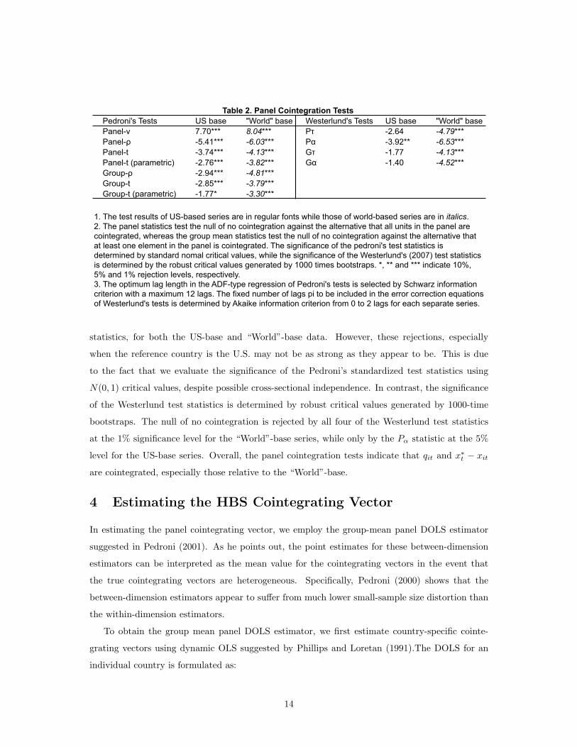
Pedroni's Tests US base "World" base Westerlund's Tests US base "World" basePanel-v 7.70*** 8.04*** Pτ -2.64 -4.79***Panel-ρ -5.41*** -6.03*** Pα -3.92** -6.53***Panel-t -3.74*** -4.13*** Gτ -1.77 -4.13***Panel-t (parametric) -2.76*** -3.82*** Gα -1.40 -4.52***Group-ρ -2.94*** -4.81***Group-t -2.85*** -3.79***Group-t (parametric) -1.77* -3.30***

Table 2. Panel Cointegration Tests

1. The test results of US-based series are in regular fonts while those of world-based series are in italics. 2. The panel statistics test the null of no cointegration against the alternative that all units in the panel are cointegrated, whereas the group mean statistics test the null of no cointegration against the alternative that at least one element in the panel is cointegrated. The significance of the pedroni's test statistics is determined by standard nomal critical values, while the significance of the Westerlund's (2007) test statistics is determined by the robust critical values generated by 1000 times bootstraps. *, ** and *** indicate 10%, 5% and 1% rejection levels, respectively. 3. The optimum lag length in the ADF-type regression of Pedroni's tests is selected by Schwarz information criterion with a maximum 12 lags. The fixed number of lags pi to be included in the error correction equations of Westerlund's tests is determined by Akaike information criterion from 0 to 2 lags for each separate series.

statistics, for both the US-base and “World”-base data. However, these rejections, especially

when the reference country is the U.S. may not be as strong as they appear to be. This is due

to the fact that we evaluate the significance of the Pedroni’s standardized test statistics using

N(0, 1) critical values, despite possible cross-sectional independence. In contrast, the significance

of the Westerlund test statistics is determined by robust critical values generated by 1000-time

bootstraps. The null of no cointegration is rejected by all four of the Westerlund test statistics

at the 1% significance level for the “World”-base series, while only by the Pα statistic at the 5%

level for the US-base series. Overall, the panel cointegration tests indicate that qit and x∗t − xitare cointegrated, especially those relative to the “World”-base.

4 Estimating the HBS Cointegrating Vector

In estimating the panel cointegrating vector, we employ the group-mean panel DOLS estimator

suggested in Pedroni (2001). As he points out, the point estimates for these between-dimension

estimators can be interpreted as the mean value for the cointegrating vectors in the event that

the true cointegrating vectors are heterogeneous. Specifically, Pedroni (2000) shows that the

between-dimension estimators appear to suffer from much lower small-sample size distortion than

the within-dimension estimators.

To obtain the group mean panel DOLS estimator, we first estimate country-specific cointe-

grating vectors using dynamic OLS suggested by Phillips and Loretan (1991).The DOLS for an

individual country is formulated as:

14

qi,t = αi + βi(xi,t − x∗t ) +pi∑

s=−pi

θi,s(∆xi,t+s −∆x∗t+s) + µi,t, (18)

where asterisk denotes either the US or the “World” counterparts. The country-specific optimal

numbers of lags and leads, pi are selected by AIC. Next we construct the group-mean panel DOLS

estimator according to Pedroni (2001), βGM = N−1∑Ni=1 βi, where βi is the DOLS estimator,

applied to the ith country of the panel. The associated t-statistic for the between-dimension

estimator above can be constructed as tβGM= N−1/2

∑Ni=1 tβi

. As can be seen clearly from the

group mean formula, the panel estimate of the cointegrating vector is an average of the estimated

individual cointegrating vectors.

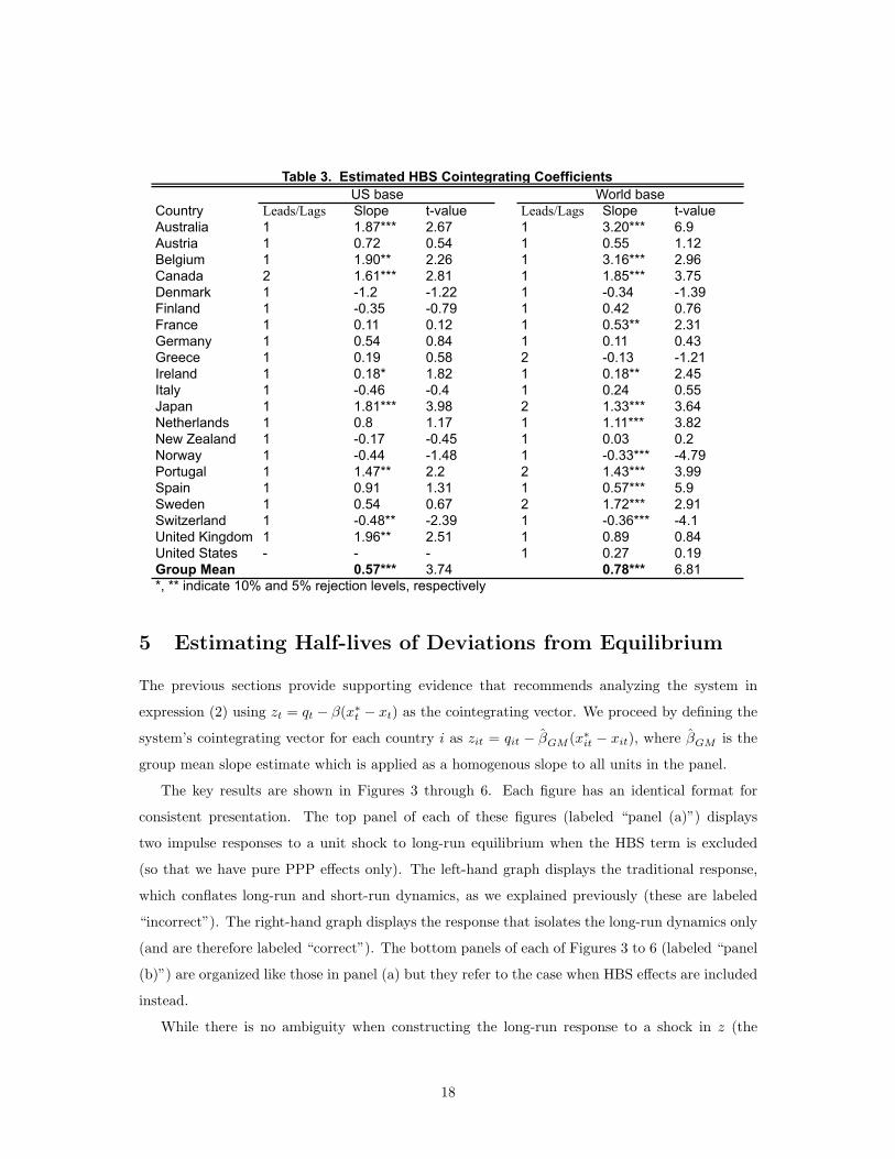
Table 3 reports the estimated individual slopes, βi, and group mean slope, βGM for our HBS

term, for the U.S. and “World” base cases. A few results are worth noting. First, the point

estimates are positive in most cases as predicted by the HBS theory, albeit they do vary greatly

among different countries. Second, the slopes estimated with the “World”-base data are in general

steeper and more significant than the corresponding ones estimated with the U.S.-base data. As

a result, the “World”-base group mean slope estimate is about twice the size of the U.S.-base one,

though both are positive and statistically significant at the 1% level.

The positive group mean estimate leads us to conclude that the HBS effect is present in the

panel, even though there is substantial variation in point estimates (and wide confidence bands)

as we look at individual countries. A slope of 0.57 for the U.S. base and 0.78 for the world base

is suggestive of an economically meaningful and qualitatively significant elasticity of price levels

with respect real income levels, and, within the range of estimation uncertainty, is consistent with

reasonable values for the share of nontraded goods in typical theoretical models of the HBS effect.

To clearly illustrate the magnitude of these effects, Figure 1(a) plots the HBS slope estimates

(individual and group mean) for the full sample using the U.S. base, where the group mean is

0.57. Figure 1(b) repeats the exercise when the panel estimation is limited to the 6 countries

(top tercile) for which the largest HBS slope coefficient is found; for this group all coefficients

are significant and the group mean slope estimate rises to 1.77. Figure 2 repeats this exercise for

the “World” base, where the group mean is 0.78 for the full sample and 1.72 in the case of the

6 top tercile countries. These results support the hypothesis that an HBS effect is present, and

although possibly heterogeneous, it could be qualitatively large in some subset of the countries

in our sample. It now remains to be seen whether the existence of such effects makes a material

difference to the methods used to assess the dynamic speed of adjustment of the real exchange

rate to its long run equilibrium value.

15

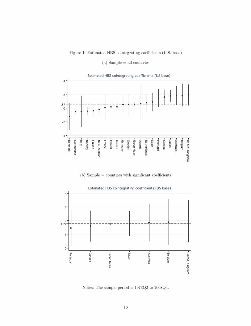
Figure 1: Estimated HBS cointegrating coefficients (U.S. base)

(a) Sample = all countries-4

-4

-4-2

-2

-20

0

02

2

24

4

4.57

.57

.57Denmark

Denmark

DenmarkSwitzerland

Switzerland

SwitzerlandItaly

Italy

ItalyNorway

Norway

NorwayFinland

Finland

FinlandNew_Zealand

New_Zealand

New_ZealandFrance

France

FranceIreland

Ireland

IrelandGreece

Greece

GreeceGermany

Germany

GermanySweden

Sweden

SwedenGroup Mean

Group Mean

Group MeanAustria

Austria

AustriaNetherlands

Netherlands

NetherlandsSpain

Spain

SpainPortugal

Portugal

PortugalCanada

Canada

CanadaJapan

Japan

JapanAustralia

Australia

AustraliaBelgium

Belgium

BelgiumUnited_KingdomUnited_Kingdom

United_KingdomUS base,73q2-08q4US base,73q2-08q4Estimated HBS cointegrating coefficients (US base)

Estimated HBS cointegrating coefficients (US base)


(b) Sample = countries with significant coefficients0

0

01

1

12

2

23

3

34

4

41.77

1.77

1.77PortugalPortugal

PortugalCanada

Canada

CanadaGroup Mean

Group Mean

Group MeanJapan

Japan

JapanAustralia

Australia

AustraliaBelgium

Belgium

BelgiumUnited_Kingdom

United_Kingdom

United_KingdomUS base,73q2-08q4US base,73q2-08q4Estimated HBS cointegrating coefficients (US base)



Notes: The sample period is 1973Q2 to 2008Q4.

16

Figure 2: Estimated HBS cointegrating coefficients (“world” base)

(a) Sample = all countries-2

-2

-20

0

02

2

24

4

46

6

6.78

.78

.78Switzerland

Switzerland

SwitzerlandDenmark

Denmark

DenmarkNorway

Norway

NorwayGreece

Greece

GreeceNew_Zealand

New_Zealand

New_ZealandGermany

Germany

GermanyIreland

Ireland

IrelandItaly

Italy

ItalyUnited_States

United_States

United_StatesFinland

Finland

FinlandFrance

France

FranceAustria

Austria

AustriaSpain

Spain

SpainGroup Mean

Group Mean

Group MeanUnited_Kingdom

United_Kingdom

United_KingdomNetherlands

Netherlands

NetherlandsJapan

Japan

JapanPortugal

Portugal

PortugalSweden

Sweden

SwedenCanada

Canada

CanadaBelgiumBelgium

BelgiumAustraliaA

ustraliaAustraliaWorld base,73q2-08q4World base,73q2-08q4Estimated HBS cointegrating coefficients (World base)

Estimated HBS cointegrating coefficients (World base)


(b) Sample = countries with significant coefficients0

0

01

1

12

2

23

3

34

4

45

5

51.72

1.72

1.72SwedenSw

edenSwedenJapan

Japan

JapanCanada

Canada

CanadaGroup Mean

Group Mean

Group MeanPortugal

Portugal

PortugalAustralia

Australia

AustraliaBelgium

Belgium

BelgiumWorld base,73q2-08q4World base,73q2-08q4Estimated HBS cointegrating coefficients (World base)



Notes: The sample period is 1973Q2 to 2008Q4.

17

Country Leads/Lags Slope t-value Leads/Lags Slope t-valueAustralia 1 1.87*** 2.67 1 3.20*** 6.9Austria 1 0.72 0.54 1 0.55 1.12Belgium 1 1.90** 2.26 1 3.16*** 2.96Canada 2 1.61*** 2.81 1 1.85*** 3.75Denmark 1 -1.2 -1.22 1 -0.34 -1.39Finland 1 -0.35 -0.79 1 0.42 0.76France 1 0.11 0.12 1 0.53** 2.31Germany 1 0.54 0.84 1 0.11 0.43Greece 1 0.19 0.58 2 -0.13 -1.21Ireland 1 0.18* 1.82 1 0.18** 2.45Italy 1 -0.46 -0.4 1 0.24 0.55Japan 1 1.81*** 3.98 2 1.33*** 3.64Netherlands 1 0.8 1.17 1 1.11*** 3.82New Zealand 1 -0.17 -0.45 1 0.03 0.2Norway 1 -0.44 -1.48 1 -0.33*** -4.79Portugal 1 1.47** 2.2 2 1.43*** 3.99Spain 1 0.91 1.31 1 0.57*** 5.9Sweden 1 0.54 0.67 2 1.72*** 2.91Switzerland 1 -0.48** -2.39 1 -0.36*** -4.1United Kingdom 1 1.96** 2.51 1 0.89 0.84United States - - - 1 0.27 0.19Group Mean 0.57*** 3.74 0.78*** 6.81

US base World baseTable 3. Estimated HBS Cointegrating Coefficients

*, ** indicate 10% and 5% rejection levels, respectively

5 Estimating Half-lives of Deviations from Equilibrium

The previous sections provide supporting evidence that recommends analyzing the system in

expression (2) using zt = qt − β(x∗t − xt) as the cointegrating vector. We proceed by defining the

system’s cointegrating vector for each country i as zit = qit − βGM (x∗it − xit), where βGM is the

group mean slope estimate which is applied as a homogenous slope to all units in the panel.

The key results are shown in Figures 3 through 6. Each figure has an identical format for

consistent presentation. The top panel of each of these figures (labeled “panel (a)”) displays

two impulse responses to a unit shock to long-run equilibrium when the HBS term is excluded

(so that we have pure PPP effects only). The left-hand graph displays the traditional response,

which conflates long-run and short-run dynamics, as we explained previously (these are labeled

“incorrect”). The right-hand graph displays the response that isolates the long-run dynamics only

(and are therefore labeled “correct”). The bottom panels of each of Figures 3 to 6 (labeled “panel

(b)”) are organized like those in panel (a) but they refer to the case when HBS effects are included

instead.

While there is no ambiguity when constructing the long-run response to a shock in z (the

18

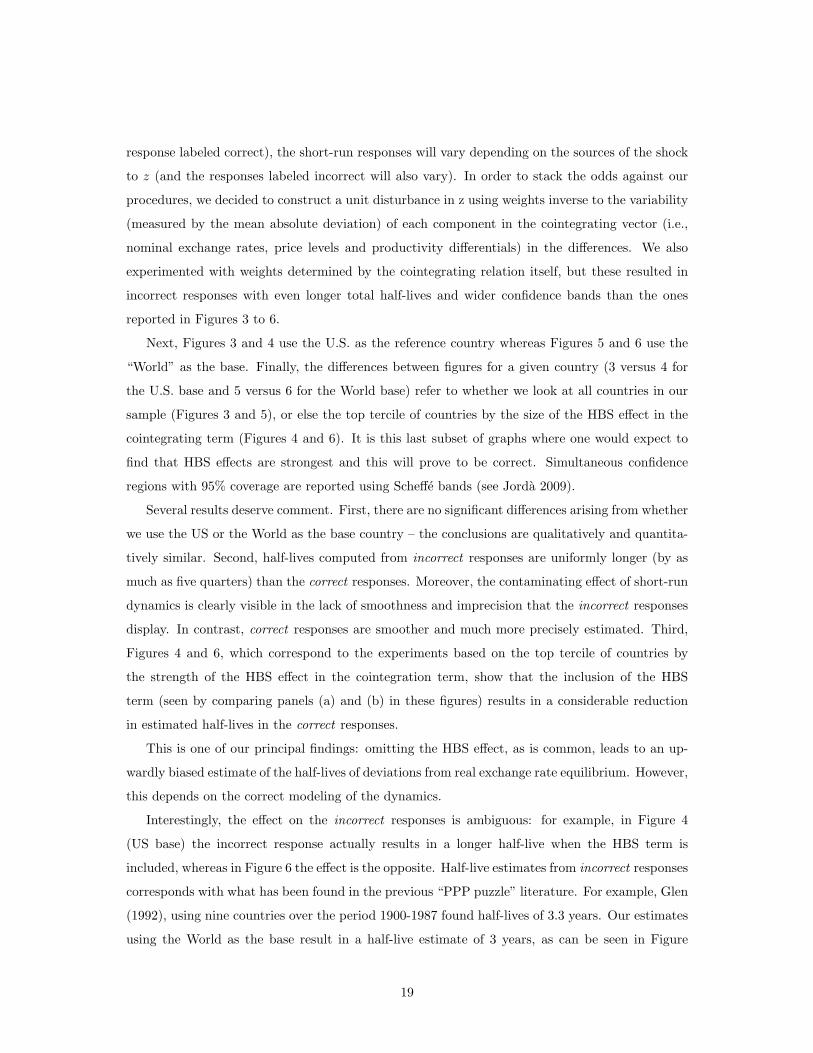
response labeled correct), the short-run responses will vary depending on the sources of the shock

to z (and the responses labeled incorrect will also vary). In order to stack the odds against our

procedures, we decided to construct a unit disturbance in z using weights inverse to the variability

(measured by the mean absolute deviation) of each component in the cointegrating vector (i.e.,

nominal exchange rates, price levels and productivity differentials) in the differences. We also

experimented with weights determined by the cointegrating relation itself, but these resulted in

incorrect responses with even longer total half-lives and wider confidence bands than the ones

reported in Figures 3 to 6.

Next, Figures 3 and 4 use the U.S. as the reference country whereas Figures 5 and 6 use the

“World” as the base. Finally, the differences between figures for a given country (3 versus 4 for

the U.S. base and 5 versus 6 for the World base) refer to whether we look at all countries in our

sample (Figures 3 and 5), or else the top tercile of countries by the size of the HBS effect in the

cointegrating term (Figures 4 and 6). It is this last subset of graphs where one would expect to

find that HBS effects are strongest and this will prove to be correct. Simultaneous confidence

regions with 95% coverage are reported using Scheffe bands (see Jorda 2009).

Several results deserve comment. First, there are no significant differences arising from whether

we use the US or the World as the base country – the conclusions are qualitatively and quantita-

tively similar. Second, half-lives computed from incorrect responses are uniformly longer (by as

much as five quarters) than the correct responses. Moreover, the contaminating effect of short-run

dynamics is clearly visible in the lack of smoothness and imprecision that the incorrect responses

display. In contrast, correct responses are smoother and much more precisely estimated. Third,

Figures 4 and 6, which correspond to the experiments based on the top tercile of countries by

the strength of the HBS effect in the cointegration term, show that the inclusion of the HBS

term (seen by comparing panels (a) and (b) in these figures) results in a considerable reduction

in estimated half-lives in the correct responses.

This is one of our principal findings: omitting the HBS effect, as is common, leads to an up-

wardly biased estimate of the half-lives of deviations from real exchange rate equilibrium. However,

this depends on the correct modeling of the dynamics.

Interestingly, the effect on the incorrect responses is ambiguous: for example, in Figure 4

(US base) the incorrect response actually results in a longer half-live when the HBS term is

included, whereas in Figure 6 the effect is the opposite. Half-live estimates from incorrect responses

corresponds with what has been found in the previous “PPP puzzle” literature. For example, Glen

(1992), using nine countries over the period 1900-1987 found half-lives of 3.3 years. Our estimates

using the World as the base result in a half-live estimate of 3 years, as can be seen in Figure

19

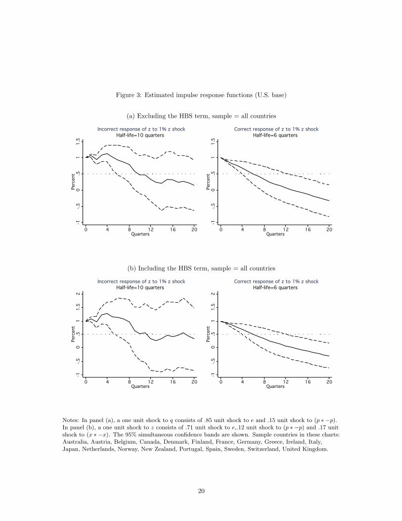
Figure 3: Estimated impulse response functions (U.S. base)

(a) Excluding the HBS term, sample = all countries-1

-1

-1-.5

-.5

-.50

0

0.5

.5

.51

1

11.5

1.5

1.5Percent

Perc

ent

Percent0

0

04

4

48

8

812

12

1216

16

1620

20

20Quarters

Quarters

QuartersHalf-life=10 quarters

Half-life=10 quarters

Half-life=10 quarters Incorrect response of z to 1% z shock

Incorrect response of z to 1% z shock

Incorrect response of z to 1% z shock-1

-1

-1-.5

-.5

-.50

0

0.5

.5

.51

1

11.5

1.5

1.5Percent

Perc

ent

Percent0

0

04

4

48

8

812

12

1216

16

1620

20

20Quarters

Quarters



Half-life=6 quarters Correct response of z to 1% z shock

Correct response of z to 1% z shock

Correct response of z to 1% z shockNotes:One unit shock to q consists of .85 unit shock to e and .15 unit shock to (p*-p).

Netherlands Norway New_Zealand Portugal Spain Sweden Switzerland United_Kingdom .US base, z=qUS base, z=q

(b) Including the HBS term, sample = all countries-1

-1

-1-.5

-.5

-.50

0

0.5

.5

.51

1

11.5

1.5

1.52

2

2Percent

Perc

ent

Percent0

0

04

4

48

8

812

12

1216

16

1620

20

20Quarters

Quarters






-1

-1-.5

-.5

-.50

0

0.5

.5

.51

1

11.5

1.5

1.52

2

2Percent

Perc

ent

Percent0

0

04

4

48

8

812

12

1216

16

1620

20

20Quarters

Quarters





Correct response of z to 1% z shockNotes:One unit shock to z consists of .97 unit shock to e,.17 unit shock to (p*-p) and .24 unit shock to (x*-x).

Netherlands Norway New_Zealand Portugal Spain Sweden Switzerland United_Kingdom .US base, z=q-.57(x*-x)US base, z=q-.57(x*-x)

Notes: In panel (a), a one unit shock to q consists of .85 unit shock to e and .15 unit shock to (p ∗ −p).In panel (b), a one unit shock to z consists of .71 unit shock to e,.12 unit shock to (p ∗ −p) and .17 unitshock to (x ∗ −x). The 95% simultaneous confidence bands are shown. Sample countries in these charts:Australia, Austria, Belgium, Canada, Denmark, Finland, France, Germany, Greece, Ireland, Italy,Japan, Netherlands, Norway, New Zealand, Portugal, Spain, Sweden, Switzerland, United Kingdom.

20

Figure 4: Estimated impulse response functions (U.S. base)

(a) Excluding the HBS term, sample = countries with significant coefficients-1

-1

-1-.5

-.5

-.50

0

0.5

.5

.51

1

11.5

1.5

1.5Percent

Perc

ent

Percent0

0

04

4

48

8

812

12

1216

16

1620

20

20Quarters

Quarters






-1

-1-.5

-.5

-.50

0

0.5

.5

.51

1

11.5

1.5

1.5Percent

Perc

ent

Percent0

0

04

4

48

8

812

12

1216

16

1620

20

20Quarters

Quarters






Australia Belgium Canada Japan United_Kingdom Portugal .

.

.US base, z=qUS base, z=q

(b) Including the HBS term, sample = countries with significant coefficients-1

-1

-1-.5

-.5

-.50

0

0.5

.5

.51

1

11.5

1.5

1.52

2

22.5

2.5

2.5Percent

Perc

ent

Percent0

0

04

4

48

8

812

12

1216

16

1620

20

20Quarters

Quarters

QuartersHalf-life=11.6 quarters

Half-life=11.6 quarters

Half-life=11.6 quarters Incorrect response of z to 1% z shock



-1

-1-.5

-.5

-.50

0

0.5

.5

.51

1

11.5

1.5

1.52

2

22.5

2.5

2.5Percent

Perc

ent

Percent0

0

04

4

48

8

812

12

1216

16

1620

20

20Quarters

Quarters





Correct response of z to 1% z shockNotes:One unit shock to z consists of 1.23 unit shock to e,.24 unit shock to (p*-p) and .26 unit shock to (x*-x).

Australia Belgium Canada Japan United_Kingdom Portugal .

.US base, z=q-1.77(x*-x)US base, z=q-1.77(x*-x)

Notes: In panel (a), a one unit shock to q consists of .84 unit shock to e and .16 unit shock to (p ∗ −p).In panel (b), a one unit shock to z consists of .71 unit shock to e,.14 unit shock to (p ∗ −p) and .15 unitshock to (x ∗ −x). The 95% simultaneous confidence bands are shown. Sample countries in these charts:Australia, Belgium, Canada, Japan, United Kingdom, Portugal.

21

Figure 5: Estimated impulse response functions (“world” base)

(a) Excluding the HBS term, sample = all countries-1

-1

-1-.5

-.5

-.50

0

0.5

.5

.51

1

11.5

1.5

1.5Percent

Perc

ent

Percent0

0

04

4

48

8

812

12

1216

16

1620

20

20Quarters

Quarters






-1

-1-.5

-.5

-.50

0

0.5

.5

.51

1

11.5

1.5

1.5Percent

Perc

ent

Percent0

0

04

4

48

8

812

12

1216

16

1620

20

20Quarters

Quarters






Netherlands Norway New_Zealand Portugal Spain Sweden Switzerland United_Kingdom United_States.World base, z=qWorld base, z=q

(b) Including the HBS term, sample = all countries-1

-1

-1-.5

-.5

-.50

0

0.5

.5

.51

1

11.5

1.5

1.52

2

2Percent

Perc

ent

Percent0

0

04

4

48

8

812

12

1216

16

1620

20

20Quarters

Quarters






-1

-1-.5

-.5

-.50

0

0.5

.5

.51

1

11.5

1.5

1.52

2

2Percent

Perc

ent

Percent0

0

04

4

48

8

812

12

1216

16

1620

20

20Quarters

Quarters






Netherlands Norway New_Zealand Portugal Spain Sweden Switzerland United_Kingdom United_States.World base, z=q-.78(x*-x)World base, z=q-.78(x*-x)

Notes: In panel (a), a one unit shock to q consists of .78 unit shock to e and .22 unit shock to (p ∗ −p).In panel (b), a one unit shock to z consists of .61 unit shock to e,.17 unit shock to (p ∗ −p) and .22 unitshock to (x ∗ −x). The 95% simultaneous confidence bands are shown. Sample countries in these charts:Australia, Austria, Belgium, Canada, Denmark, Finland, France, Germany, Greece, Ireland, Italy,Japan, Netherlands, Norway, New Zealand, Portugal, Spain, Sweden, Switzerland, United Kingdom.

22

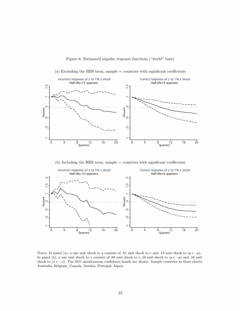
Figure 6: Estimated impulse response functions (“world” base)

(a) Excluding the HBS term, sample = countries with significant coefficients-1

-1

-1-.5

-.5

-.50

0

0.5

.5

.51

1

11.5

1.5

1.5Percent

Perc

ent

Percent0

0

04

4

48

8

812

12

1216

16

1620

20

20Quarters

Quarters






-1

-1-.5

-.5

-.50

0

0.5

.5

.51

1

11.5

1.5

1.5Percent

Perc

ent

Percent0

0

04

4

48

8

812

12

1216

16

1620

20

20Quarters

Quarters






Australia Belgium Canada Sweden Portugal Japan.World base, z=qWorld base, z=q

(b) Including the HBS term, sample = countries with significant coefficients-1

-1

-1-.5

-.5

-.50

0

0.5

.5

.51

1

11.5

1.5

1.52

2

2Percent

Perc

ent

Percent0

0

04

4

48

8

812

12

1216

16

1620

20

20Quarters

Quarters






-1

-1-.5

-.5

-.50

0

0.5

.5

.51

1

11.5

1.5

1.52

2

2Percent

Perc

ent

Percent0

0

04

4

48

8

812

12

1216

16

1620

20

20Quarters

Quarters






Australia Belgium Canada Sweden Portugal Japa

.World base, z=q-1.72(x*-x)World base, z=q-1.72(x*-x)

Notes: In panel (a), a one unit shock to q consists of .81 unit shock to e and .19 unit shock to (p ∗ −p).In panel (b), a one unit shock to z consists of .68 unit shock to e,.16 unit shock to (p ∗ −p) and .16 unitshock to (x ∗ −x). The 95% simultaneous confidence bands are shown. Sample countries in these charts:Australia, Belgium, Canada, Sweden, Portugal, Japan.

23

5(b). Taylor (2002), using 20 countries (mostly in the OECD) for the period 1850-1996 reports

mean and median half-lives of 2-3 years. Using more complex nonlinear specifications based on

an exponential smooth transition model, Peel, Sarno and Taylor (2001) found half-lives in the

3-5year range using four bilateral dollar exchange rates for the recent free floating period.

These results are reassuring because they suggest that neither the use of a local projection

estimator; the specific cross-section of countries considered; the time period used; the frequency

of the data; the linearity of the specification; nor the country used as base explain the differences

between the literature and our findings. Rather, the main result that half-lives are about three

to five quarters shorter than previously estimated is driven primarily by correctly allowing for

the contribution of the HBS effect to long-run equilibrium adjustment. And to this end, it is

important to isolate the contaminating effects of short-run frictions, which our local projection

estimator for cointegrated systems clearly shows how to do.

6 Conclusion

Models of open economies describe the behavior of aggregate variables over medium- and long-run

frequencies meant to reflect the time-scale of relevant policy questions. A central ingredient of

such models is an assumptions about how secular movements in exchange rates are determined.

In this respect, it has been traditional to focus on equilibrium conditions in fully flexible and

frictionless markets, such as the well-known PPP and UIP conditions. While basic and powerful,

these mechanisms have found precarious support in the data.

Harrod (1933), Balassa (1964) and Samuelson (1964) extended the notion of the PPP conditions

to account for differences in the traded/non-traded sectors across economies that may persist over

time due to differences in productivity. This paper investigates whether this mechanism provides

sufficient texture to explain movements of exchange rates in the long-run by introducing new

empirical methods whose applicability transcends this paper.

We take the view that there are many factors that influence exchange rates but we are interested

in those whose effects are felt over the long-run rather than those whose effects are short-lived.

The methods that we introduce are not simply another way of answering this question: they

provide a decomposition of the data that is central to obtaining the correct answer.

The local projection approach serves to formulate how one can measure adjustment to long-run

equilibrium in terms of the intrinsic long-run dynamics that the PPP/HBS hypothesis generates

from all other factors whose role is limited to explain short-run movements. Previous studies do

not make this distinction and hence provide contaminated measures of the HBS hypothesis. Not

surprisingly, we find that empirical estimates of half-lives are considerably shorter than what has

24

been previously reported. Such finding provide support not only for the HBS hypothesis, but also

for the view that equilibrium adjustment speeds are not so puzzling.

The local projection approach for cointegrated systems is an important econometric contribu-

tion in its own right. The methods not only proved useful in our application but also open the

door for more sophisticated analysis of non-linear error correction adjustments that have been

hitherto complicated by the need to specify nonlinear stochastic processes for the entire system of

variables considered. It is our hope that this paper will also help to illustrate the advantages of

this approach and inspire further applications.

References

Javier Alvarez and Manuel Arellano (2003) ”The Time Series and Cross-Section Asymptotics of

Dynamic Panel Data Estimators,” Econometrica, Econometric Society, vol. 71(4), pages 1121-1159,

07.

Arellano, Manuel and Bond, Stephen (1991) ”Some Tests of Specification for Panel Data: Monte

Carlo Evidence and an Application to Employment Equations,” Review of Economic Studies, Black-

well Publishing, vol. 58(2), pages 277-97, April.

Balassa, Bela (1964) “The Purchasing-Power Parity Doctrine: A Reappraisal” , Journal of Political

Economy, 72, 584-596.

Banerjee, A., J. J. Dolado, and R. Mestre (1998) “Error-correction Mechanism Tests for Cointegra-

tion in a Single-equation Framework,” Journal of Time Series Analysis, 19, 3, 267-283.

Menzie Chinn & Louis Johnston, 1996. “Real Exchange Rate Levels, Productivity and Demand

Shocks: Evidence from a Panel of 14 Countries,” NBER Working Papers 5709, National Bureau of

Economic Research, Inc.

Elliott, Graham, Thomas J. Rothenberg and James H. Stock (1996) “Efficient Tests for an Autore-

gressive Unit Root,” Econometrica, Vol. 64, No. 4, 813-836.

Ehsan U. Choudhri & Mohsin S. Khan, 2005. “Real Exchange Rates in Developing Countries: Are

Balassa-Samuelson Effects Present?,” IMF Staff Papers, Palgrave Macmillan Journals, vol. 52(3),

pages 2.

Jeffrey A. Frankel (1986) “International Capital Mobility and Crowding Out in the U.S. Economy:

Imperfect Integration of Financial Markets or of Goods Markets?,” NBER Working Papers 1773,

National Bureau of Economic Research, Inc.

Glen, J.H., (1992) “Real Exchange Rates in the Short, Medium, and Long Run” , Journal of

International Economics 33, 147-66.

Laszlo Halpern & Charles Wyplosz, 2001. “Economic Transformation and Real Exchange Rates in

the 2000s: The Balassa-Samuelson Connection,” ECE Discussion Papers Series 2001.1, UNECE.

Hamilton, James D. (1994) Time Series Analysis. Princeton University Press.

Harrod, Roy F (1933) International Economics, Nisbet & Cambridge University Press.

25

Takatoshi Ito, Peter Isard, and Steven Symansky, 1999. ”Economic Growth and Real Exchange

Rate: An Overview of the Balassa-Samuelson Hypothesis in Asia,” NBER Chapters, in: Changes

in Exchange Rates in Rapidly Development Countries: Theory, Practice, and Policy Issues (NBER-

EASE volume 7), pages 109-132 National Bureau of Economic Research, Inc.

Oscar Jorda (2005) “Estimation and Inference of Impulse Responses by Local Projections,” Amer-

ican Economic Review, 95(1), 161-182.

Oscar Jorda (2009) “Simultaneous Confidence Regions for Impulse Responses,” The Review of

Economics and Statistics, August 2009, 91(3): 629–647.

Oscar Jorda and Sharon Kozicki (2010) ”Estimation and Inference by the Method of Projection

Minimum Distance: An Application to the New Keynesian Hybrid Phillips Curve,” International

Economic Review, forthcoming.

Jeroen J.M. Kremers, Neil R. Ericsson, and Juan J. Dolado (1992) “The power of cointegration

tests,” International Finance Discussion Papers 431, Board of Governors of the Federal Reserve

System (U.S.).

Jaewoo Lee and Man-Keung Tang, 2007. “Does Productivity Growth Appreciate the Real Exchange

Rate?,” Review of International Economics, Blackwell Publishing, vol. 15(1), pages 164-187, 02.

Lewis, R. and G. Reinsel (1985) “Prediction of Multivariate Time Series by Autoregressive Model

Fitting,” Journal of Multivariate Analysis, 16, 393-411.

JamesR. Lothian & MarkP. Taylor, 2008. “Real Exchange Rates Over the Past Two Centuries: How

Important is the Harrod-Balassa-Samuelson Effect?,” Economic Journal, Royal Economic Society,

vol. 118(532), pages 1742-1763, October.

Nickell, Stephen J. (1981) “Biases in Dynamic Models with Fixed Effects,” Econometrica, Econo-

metric Society, vol. 49(6), pages 1417-26, November.

Paul G. J. O’Connell (1998) “The overvaluation of purchasing power parity,” Journal of Interna-

tional Economics, Volume 44, Issue 1, 1 February 1998, Pages 1-19.

Pedroni, P (1999) “Critical values for cointegration tests in heterogenous panels with multiple

regressors” , Oxford Bulletin of Economics and Statistics, 61, 653-678.

Pedroni, P. (2000) “Fully Modified OLS for Heterogeneous Cointegrated Panels” , Advances in

Econometrics, 15 (2000), 93–130.

Pedroni, P. (2001) “Purchasing power parity tests in cointegrated panels” , The Review of Economics

and Statistics, Vol. 83(4), 727–731.

Pedroni, P. (2004) “Panel Cointegration. Asymptotic and Finite Sample Properties of Pooled Time

Series Tests with an Application to the PPP Hypothesis” , Econometric Theory, 20, 200, 597–625.

Peel, David, Sarno, Lucio, and Taylor, Mark P (2001) “Nonlinear Mean-Reversion in Real Exchange

Rates: Towards a Solution to the Purchasing Power Parity Puzzles,” CEPR Discussion Papers 2658,

C.E.P.R. Discussion Papers.

Damiaan Persyn and Joakim Westerlund, 2008. ”XTWEST: Stata module for testing for cointegra-

tion in heterogeneous panels,” Statistical Software Components S456941, Boston College Depart-

ment of Economics.

Pesaran, M.H. (2003) “A Simple Panel Unit Root Test in the Presence of Cross Section Dependence,”

Cambridge Working Papers in Economics 0346, Faculty of Economics, University of Cambridge.

26

Phillips,P.C.B. and Mico Loretan (1991) “Estimating Long-Run Economic Equilibria,” The Review

of Economic Studies, Vol. 58, No. 3, Special Issue: The Econometrics of Financial Markets, 407-436.

Phillips, Peter C. B., and Pierre Perron (1988) “Testing for a Unit Root in Time Series Regression.”

, Biometrika, 75, 335-46.

Phillips, P.C.B. and S. Ouliaris (1990) “Asymptotic Properties of Residual Based Tests forCointe-

gration.” , Econometrica 58, 165–193.

Samuelson, P.A. (1964) “Theoretical Notes on Trade Problems” , Review of Economics and Statis-

tics, Vol. 46, No. 1, pp 145-154.

Alan M. Taylor (2002) “A Century of Purchasing-Power Parity,” The Review of Economics and

Statistics, February 2002, 84(1): 139–150.

Alan M. Taylor, and Mark P. Taylor (2004) “The Purchasing Power Parity Debate,” Journal of

Economic Perspectives, American Economic Association, vol. 18(4), pages 135-158, Fall.

Joakim Westerlund (2007) “Testing for Error Correction in Panel Data,” Oxford Bulletin of Eco-

nomics and Statistics, 69, 6 (2007) 0305-9049.

Appendix A: Raw Data

Figures A1 and A2 show the raw data for log real exchange rates and log relative GDP per capita for the

U.S. and world bases, respectively.

27

Figure A11.2

1.2

1.21.25

1.25

1.251.3

1.3

1.31.35

1.35

1.35x-x*

x-x*

x-x*00

0.5.5

.511

1qq

q1973q2

1973q2

1973q21983q2

1983q2

1983q21993q2

1993q2

1993q22003q2

2003q2

2003q22013q2

2013q2

2013q2Australia

Australia

Australia-1

-1

-1-.95

-.95

-.95-.9

-.9

-.9-.85

-.85

-.85x-x*

x-x*

x-x*2

2

22.5

2.5

2.53

3

3q

q

q1973q2

1973q2

1973q21983q2

1983q2

1983q21993q2

1993q2

1993q22003q2

2003q2

2003q22013q2

2013q2

2013q2Austria

Austria

Austria-2.05

-2.0

5

-2.05-2

-2

-2-1.95

-1.9

5

-1.95-1.9

-1.9

-1.9x-x*

x-x*

x-x*3

3

33.5

3.5

3.54

4

4q

q

q1973q2

1973q2

1973q21983q2

1983q2

1983q21993q2

1993q2

1993q22003q2

2003q2

2003q22013q2

2013q2

2013q2Belgium

Belgium

Belgium-.05

-.05

-.050

0

0.05

.05

.05.1

.1

.1x-x*

x-x*

x-x*00

0.2.2

.2.4.4

.4qq

q1973q2

1973q2

1973q21983q2

1983q2

1983q21993q2

1993q2

1993q22003q2

2003q2

2003q22013q2

2013q2

2013q2Canada

Canada

Canada-.65

-.65

-.65-.6

-.6

-.6-.55

-.55

-.55x-x*

x-x*

x-x*1.5

1.5

1.52

2

22.5

2.5

2.5q

q

q1973q2

1973q2

1973q21983q2

1983q2

1983q21993q2

1993q2

1993q22003q2

2003q2

2003q22013q2

2013q2

2013q2Denmark

Denmark

Denmark-.2

-.2

-.2-.1

-.1

-.10

0

0.1

.1

.1x-x*

x-x*

x-x*1

1

11.5

1.5

1.52

2

2q

q

q1973q2

1973q2

1973q21983q2

1983q2

1983q21993q2

1993q2

1993q22003q2

2003q2

2003q22013q2

2013q2

2013q2Finland

Finland

Finland-.3

-.3

-.3-.2

-.2

-.2-.1

-.1

-.1x-x*

x-x*

x-x*1.41.

41.41.6

1.6

1.61.81.

81.82

22q

qq1973q2

1973q2

1973q21983q2

1983q2

1983q21993q2

1993q2

1993q22003q2

2003q2

2003q22013q2

2013q2

2013q2France

France

France-6.6

-6.6

-6.6-6.5

-6.5

-6.5-6.4

-6.4

-6.4x-x*

x-x*

x-x*0

0

0.5

.5

.51

1

1q

q

q1973q2

1973q2

1973q21983q2

1983q2

1983q21993q2

1993q2

1993q22003q2

2003q2

2003q22013q2

2013q2

2013q2Germany

Germany

Germany-3.8

-3.8

-3.8-3.6

-3.6

-3.6-3.4

-3.4

-3.4x-x*

x-x*

x-x*5.5

5.5

5.56

6

66.5

6.5

6.5q

q

q1973q2

1973q2

1973q21983q2

1983q2

1983q21993q2

1993q2

1993q22003q2

2003q2

2003q22013q2

2013q2

2013q2Greece

Greece

Greece-5.5

-5.5

-5.5-5

-5

-5-4.5

-4.5

-4.5x-x*

x-x*

x-x*-1-1

-1-.5-.5

-.500

0qq

q1973q2

1973q2

1973q21983q2

1983q2

1983q21993q2

1993q2

1993q22003q2

2003q2

2003q22013q2

2013q2

2013q2Ireland

Ireland

Ireland1.15

1.15

1.151.2

1.2

1.21.25

1.25

1.251.3

1.3

1.3x-x*

x-x*

x-x*7

7

77.5

7.5

7.58

8

8q

q

q1973q2

1973q2

1973q21983q2

1983q2

1983q21993q2

1993q2

1993q22003q2

2003q2

2003q22013q2

2013q2

2013q2Italy

Italy

Italy-4.8

-4.8

-4.8-4.7

-4.7

-4.7-4.6

-4.6

-4.6-4.5

-4.5

-4.5x-x*

x-x*

x-x*4

4

44.5

4.5

4.55

5

5q

q

q1973q2

1973q2

1973q21983q2

1983q2

1983q21993q2

1993q2

1993q22003q2

2003q2

2003q22013q2

2013q2

2013q2Japan

Japan

Japan.75

.75

.75.8

.8

.8.85

.85

.85.9

.9

.9x-x*

x-x*

x-x*.4.4

.4.6.6

.6.8.8

.811

1qq

q1973q2

1973q2

1973q21983q2

1983q2

1983q21993q2

1993q2

1993q22003q2

2003q2

2003q22013q2

2013q2

2013q2Netherlands

Netherlands

Netherlands-1

-1

-1-.8

-.8

-.8-.6

-.6

-.6x-x*

x-x*

x-x*1.6

1.6

1.61.8

1.8

1.82

2

22.2

2.2

2.2q

q

q1973q2

1973q2

1973q21983q2

1983q2

1983q21993q2

1993q2

1993q22003q2

2003q2

2003q22013q2

2013q2

2013q2Norway

Norway

Norway-5.8

-5.8

-5.8-5.6

-5.6

-5.6-5.4

-5.4

-5.4x-x*

x-x*

x-x*0

0

0.5

.5

.51

1

1q

q

q1973q2

1973q2

1973q21983q2

1983q2

1983q21993q2

1993q2

1993q22003q2

2003q2

2003q22013q2

2013q2

2013q2New_Zealand

New_Zealand

New_Zealand-2.9

-2.9

-2.9-2.8

-2.8

-2.8-2.7

-2.7

-2.7x-x*

x-x*

x-x*55

55.55.

55.56

66q

qq1973q2

1973q2

1973q21983q2

1983q2

1983q21993q2

1993q2

1993q22003q2

2003q2

2003q22013q2

2013q2

2013q2Portugal

Portugal

Portugal-3.1

-3.1

-3.1-3

-3

-3-2.9

-2.9

-2.9x-x*

x-x*

x-x*4.5

4.5

4.55

5

55.5

5.5

5.5q

q

q1973q2

1973q2

1973q21983q2

1983q2

1983q21993q2

1993q2

1993q22003q2

2003q2

2003q22013q2

2013q2

2013q2Spain

Spain

Spain-.7

-.7

-.7-.6

-.6

-.6-.5

-.5

-.5x-x*

x-x*

x-x*1.5

1.5

1.52

2

22.5

2.5

2.5q

q

q1973q2

1973q2

1973q21983q2

1983q2

1983q21993q2

1993q2

1993q22003q2

2003q2

2003q22013q2

2013q2

2013q2Sweden

Sweden

Sweden.6

.6

.6.8

.8

.81

1

1x-x*

x-x*

x-x*00

0.5.5

.511

1qq

q1973q2

1973q2

1973q21983q2

1983q2

1983q21993q2

1993q2

1993q22003q2

2003q2

2003q22013q2

2013q2

2013q2Switzerland

Switzerland

Switzerland2

2

22.1

2.1

2.12.2

2.2

2.2x-x*

x-x*

x-x*-1

-1

-1-.5

-.5

-.50

0

0q

q

q1973q2

1973q2

1973q21983q2

1983q2

1983q21993q2

1993q2

1993q22003q2

2003q2

2003q22013q2

2013q2

2013q2United_Kingdom

United_Kingdom

United_Kingdom Note: Solid blue lines represent log real exchange rates,

Note: Solid blue lines represent log real exchange rates,

Note: Solid blue lines represent log real exchange rates, and Dashed red colored lines represent log real GDP per capita

and Dashed red colored lines represent log real GDP per capita

and Dashed red colored lines represent log real GDP per capitaIFS data:US-Based Log Real Exchange Rates and Log Per Capita Output Ratios

IFS data:US-Based Log Real Exchange Rates and Log Per Capita Output Ratios

IFS data:US-Based Log Real Exchange Rates and Log Per Capita Output Ratios

28

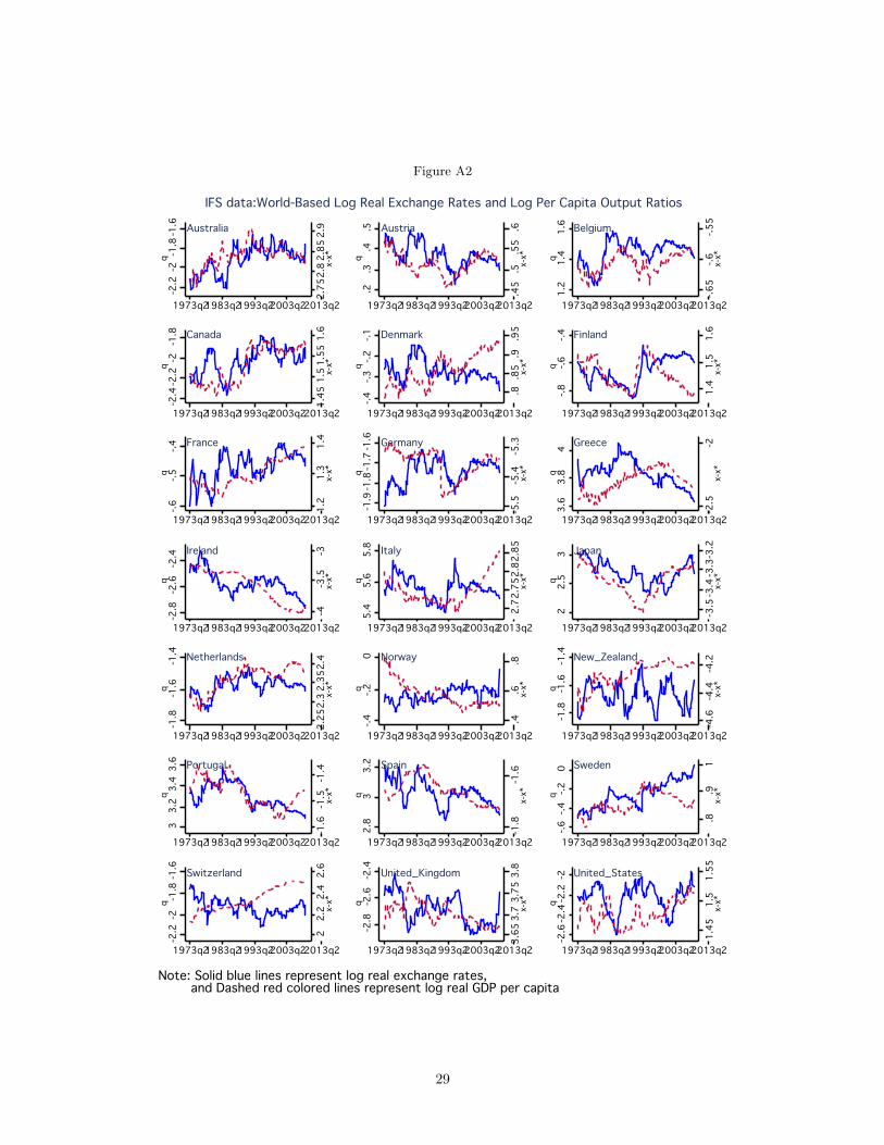
Figure A22.75

2.75

2.752.8

2.8

2.82.85

2.85

2.852.9

2.9

2.9x-x*

x-x*

x-x*-2.2-2

.2-2.2-2

-2-2-1.8

-1.8

-1.8-1.6-1

.6-1.6q

qq1973q2

1973q2

1973q21983q2

1983q2

1983q21993q2

1993q2

1993q22003q2

2003q2

2003q22013q2

2013q2

2013q2Australia

Australia

Australia.45

.45

.45.5

.5

.5.55

.55

.55.6

.6

.6x-x*

x-x*

x-x*.2

.2

.2.3

.3

.3.4

.4

.4.5

.5

.5q

q

q1973q2

1973q2

1973q21983q2

1983q2

1983q21993q2

1993q2

1993q22003q2

2003q2

2003q22013q2

2013q2

2013q2Austria

Austria

Austria-.65

-.65

-.65-.6

-.6

-.6-.55

-.55

-.55x-x*

x-x*

x-x*1.2

1.2

1.21.4

1.4

1.41.6

1.6

1.6q

q

q1973q2

1973q2

1973q21983q2

1983q2

1983q21993q2

1993q2

1993q22003q2

2003q2

2003q22013q2

2013q2

2013q2Belgium

Belgium

Belgium1.45

1.45

1.451.5

1.5

1.51.55

1.55

1.551.6

1.6

1.6x-x*

x-x*

x-x*-2.4-2

.4-2.4-2.2

-2.2

-2.2-2-2

-2-1.8-1

.8-1.8q

qq1973q2

1973q2

1973q21983q2

1983q2

1983q21993q2

1993q2

1993q22003q2

2003q2

2003q22013q2

2013q2

2013q2Canada

Canada

Canada.8

.8

.8.85

.85

.85.9

.9

.9.95

.95

.95x-x*

x-x*

x-x*-.4

-.4

-.4-.3

-.3

-.3-.2

-.2

-.2-.1

-.1

-.1q

q

q1973q2

1973q2

1973q21983q2

1983q2

1983q21993q2

1993q2

1993q22003q2

2003q2

2003q22013q2

2013q2

2013q2Denmark

Denmark

Denmark1.4

1.4

1.41.5

1.5

1.51.6

1.6

1.6x-x*

x-x*

x-x*-.8

-.8

-.8-.6

-.6

-.6-.4

-.4

-.4q

q

q1973q2

1973q2

1973q21983q2

1983q2

1983q21993q2

1993q2

1993q22003q2

2003q2

2003q22013q2

2013q2

2013q2Finland

Finland

Finland1.2

1.2

1.21.3

1.3

1.31.4

1.4

1.4x-x*

x-x*

x-x*-.6-.6

-.6-.5-.5

-.5-.4-.4

-.4qq

q1973q2

1973q2

1973q21983q2

1983q2

1983q21993q2

1993q2

1993q22003q2

2003q2

2003q22013q2

2013q2

2013q2France

France

France-5.5

-5.5

-5.5-5.4

-5.4

-5.4-5.3

-5.3

-5.3x-x*

x-x*

x-x*-1.9

-1.9

-1.9-1.8

-1.8

-1.8-1.7

-1.7

-1.7-1.6

-1.6

-1.6q

q

q1973q2

1973q2

1973q21983q2

1983q2

1983q21993q2

1993q2

1993q22003q2

2003q2

2003q22013q2

2013q2

2013q2Germany

Germany

Germany-2.5

-2.5

-2.5-2

-2

-2x-x*

x-x*

x-x*3.6

3.6

3.63.8

3.8

3.84

4

4q

q

q1973q2

1973q2

1973q21983q2

1983q2

1983q21993q2

1993q2

1993q22003q2

2003q2

2003q22013q2

2013q2

2013q2Greece

Greece

Greece-4

-4

-4-3.5

-3.5

-3.5-3

-3

-3x-x*

x-x*

x-x*-2.8-2

.8-2.8-2.6

-2.6

-2.6-2.4-2

.4-2.4q

qq1973q2

1973q2

1973q21983q2

1983q2

1983q21993q2

1993q2

1993q22003q2

2003q2

2003q22013q2

2013q2

2013q2Ireland

Ireland

Ireland2.7

2.7

2.72.75

2.75

2.752.8

2.8

2.82.85

2.85

2.85x-x*

x-x*

x-x*5.4

5.4

5.45.6

5.6

5.65.8

5.8

5.8q

q

q1973q2

1973q2

1973q21983q2

1983q2

1983q21993q2

1993q2

1993q22003q2

2003q2

2003q22013q2

2013q2

2013q2Italy

Italy

Italy-3.5

-3.5

-3.5-3.4

-3.4

-3.4-3.3

-3.3

-3.3-3.2

-3.2

-3.2x-x*

x-x*

x-x*2

2

22.5

2.5

2.53

3

3q

q

q1973q2

1973q2

1973q21983q2

1983q2

1983q21993q2

1993q2

1993q22003q2

2003q2

2003q22013q2

2013q2

2013q2Japan

Japan

Japan2.25

2.25

2.252.3

2.3

2.32.35

2.35

2.352.4

2.4

2.4x-x*

x-x*

x-x*-1.8-1

.8-1.8-1.6

-1.6

-1.6-1.4-1

.4-1.4q

qq1973q2

1973q2

1973q21983q2

1983q2

1983q21993q2

1993q2

1993q22003q2

2003q2

2003q22013q2

2013q2

2013q2Netherlands

Netherlands

Netherlands.4

.4

.4.6

.6

.6.8

.8

.8x-x*

x-x*

x-x*-.4

-.4

-.4-.2

-.2

-.20

0

0q

q

q1973q2

1973q2

1973q21983q2

1983q2

1983q21993q2

1993q2

1993q22003q2

2003q2

2003q22013q2

2013q2

2013q2Norway

Norway

Norway-4.6

-4.6

-4.6-4.4

-4.4

-4.4-4.2

-4.2

-4.2x-x*

x-x*

x-x*-1.8

-1.8

-1.8-1.6

-1.6

-1.6-1.4

-1.4

-1.4q

q

q1973q2

1973q2

1973q21983q2

1983q2

1983q21993q2

1993q2

1993q22003q2

2003q2

2003q22013q2

2013q2

2013q2New_Zealand

New_Zealand

New_Zealand-1.6

-1.6

-1.6-1.5

-1.5

-1.5-1.4

-1.4

-1.4x-x*

x-x*

x-x*33

33.23.

23.23.4

3.4

3.43.63.

63.6q

qq1973q2

1973q2

1973q21983q2

1983q2

1983q21993q2

1993q2

1993q22003q2

2003q2

2003q22013q2

2013q2

2013q2Portugal

Portugal

Portugal-1.8

-1.8

-1.8-1.6

-1.6

-1.6x-x*

x-x*

x-x*2.8

2.8

2.83

3

33.2

3.2

3.2q

q

q1973q2

1973q2

1973q21983q2

1983q2

1983q21993q2

1993q2

1993q22003q2

2003q2

2003q22013q2

2013q2

2013q2Spain

Spain

Spain.8

.8

.8.9

.9

.91

1

1x-x*

x-x*

x-x*-.6

-.6

-.6-.4

-.4

-.4-.2

-.2

-.20

0

0q

q

q1973q2

1973q2

1973q21983q2

1983q2

1983q21993q2

1993q2

1993q22003q2

2003q2

2003q22013q2

2013q2

2013q2Sweden

Sweden

Sweden2

2

22.2

2.2

2.22.4

2.4

2.42.6

2.6

2.6x-x*

x-x*

x-x*-2.2-2

.2-2.2-2

-2-2-1.8

-1.8

-1.8-1.6-1

.6-1.6q

qq1973q2

1973q2

1973q21983q2

1983q2

1983q21993q2

1993q2

1993q22003q2

2003q2

2003q22013q2

2013q2

2013q2Switzerland

Switzerland

Switzerland3.65

3.65

3.653.7

3.7

3.73.75

3.75

3.753.8

3.8

3.8x-x*

x-x*

x-x*-2.8

-2.8

-2.8-2.6

-2.6

-2.6-2.4

-2.4

-2.4q

q

q1973q2

1973q2

1973q21983q2

1983q2

1983q21993q2

1993q2

1993q22003q2

2003q2

2003q22013q2

2013q2

2013q2United_Kingdom

United_Kingdom

United_Kingdom1.45

1.45

1.451.5

1.5

1.51.55

1.55

1.55x-x*

x-x*

x-x*-2.6

-2.6

-2.6-2.4

-2.4

-2.4-2.2

-2.2

-2.2-2

-2

-2q

q

q1973q2

1973q2

1973q21983q2

1983q2

1983q21993q2

1993q2

1993q22003q2

2003q2

2003q22013q2

2013q2

2013q2United_States

United_States

United_States Note: Solid blue lines represent log real exchange rates,

Note: Solid blue lines represent log real exchange rates,

Note: Solid blue lines represent log real exchange rates, and Dashed red colored lines represent log real GDP per capita

and Dashed red colored lines represent log real GDP per capita

and Dashed red colored lines represent log real GDP per capitaIFS data:World-Based Log Real Exchange Rates and Log Per Capita Output Ratios

IFS data:World-Based Log Real Exchange Rates and Log Per Capita Output Ratios

IFS data:World-Based Log Real Exchange Rates and Log Per Capita Output Ratios

29

The Harrod-Balassa-Samuelson Hypothesis: Real Exchange ... · The Harrod-Balassa-Samuelson...

Documents

Transcript of The Harrod-Balassa-Samuelson Hypothesis: Real Exchange ... · The Harrod-Balassa-Samuelson...