Epidemic Modelling Intro
62
1/62 1 Epidemic Modelling Intro Instructor: David Earn Mathematics 747 / 5GT3 Topics in Mathematical Biology
Transcript of Epidemic Modelling Intro

1/62
1 Epidemic Modelling Intro
Instructor: David Earn Mathematics 747 / 5GT3 Topics in Mathematical Biology

Epidemic Modelling Intro 2/62
Mathematicsand Statistics∫M
dω =∫∂M
ω
Mathematics 747 / 5GT3Topics in Mathematical Biology
Instructor: David Earn
Lecture 1Epidemic Modelling Intro
Thursday 17 September 2020
Instructor: David Earn Mathematics 747 / 5GT3 Topics in Mathematical Biology

Epidemic Modelling Intro Course Information 3/62
Course information
The course web site:http://davidearn.github.io/tmb2020
Office hours are by appointment (online only):E-mail [email protected]
Instructor: David Earn Mathematics 747 / 5GT3 Topics in Mathematical Biology

Epidemic Modelling Intro Software 4/62
Software
ASAP, install the software discussed on the Software page onthe course web site:
LATEX
R
RStudioEmacs
Note: the Software page also contains some info aboutspell-checking and counting words in LATEX documents.
Instructor: David Earn Mathematics 747 / 5GT3 Topics in Mathematical Biology

Epidemic Modelling Intro Attendance 5/62
Attendance
Who is here?
Instructor: David Earn Mathematics 747 / 5GT3 Topics in Mathematical Biology

Epidemic Modelling Intro 6/62
EpidemicModelling
Instructor: David Earn Mathematics 747 / 5GT3 Topics in Mathematical Biology

Epidemic Modelling Intro Examples of Epidemic Data 7/62
Daily SARS-CoV-1 in 2003 (Worldwide)
Apr May Jun Jul
0
200
400
600
800
Dai
ly n
ew c
ases
8265 cases809 deaths
Instructor: David Earn Mathematics 747 / 5GT3 Topics in Mathematical Biology

Epidemic Modelling Intro Examples of Epidemic Data 8/62
Daily SARS-CoV-2 in 2020 (Worldwide)
Jan Mar May Jul Sep
0
50000
100000
150000
200000
250000
300000
Instructor: David Earn Mathematics 747 / 5GT3 Topics in Mathematical Biology

Epidemic Modelling Intro Examples of Epidemic Data 9/62
Daily SARS-CoV-1 vs SARS-CoV-2 (Worldwide)
0 50 100 150 200 250
1
100
10000
Days since first reported case
Dai
ly n
ew c
ases
SARS−CoV−2 (2020)SARS−CoV−1 (2003)
Instructor: David Earn Mathematics 747 / 5GT3 Topics in Mathematical Biology

Epidemic Modelling Intro Examples of Epidemic Data 10/62
Daily SARS-CoV-2 (Worldwide) exponential growth fits
Jan Feb Mar Apr May Jun Jul Aug Sep2020
5 × 10²
103
2 × 10³
5 × 10³
104
2 × 10⁴
5 × 10⁴
105
2 × 10⁵
New
con
firm
atio
ns Doubling Time
Jan−Feb: ~6 daysMarch: ~5 daysMay−July: ~45 days
Instructor: David Earn Mathematics 747 / 5GT3 Topics in Mathematical Biology

Epidemic Modelling Intro Examples of Epidemic Data 11/62
Pneumonia & Influenza Mortality, Philadelphia, 1918
Sep Oct Nov Dec
0
200
400
600
800
P&I Deaths
Date
Instructor: David Earn Mathematics 747 / 5GT3 Topics in Mathematical Biology
Epidemic Modelling Intro Constructing a model 12/62
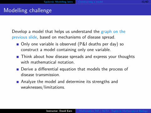
Modelling challenge
Develop a model that helps us understand the graph on theprevious slide, based on mechanisms of disease spread.
Only one variable is observed (P&I deaths per day) soconstruct a model containing only one variable.Think about how disease spreads and express your thoughtswith mathematical notation.Derive a differential equation that models the process ofdisease transmission.Analyze the model and determine its strengths andweaknesses/limitations.
Instructor: David Earn Mathematics 747 / 5GT3 Topics in Mathematical Biology

Epidemic Modelling Intro Constructing a model 13/62
Make (Biological) Assumptions Clear
1 Assume the disease is transmitted by contact between aninfected individual and a susceptible individual.
2 Assume the latent period (delay between being infected andbecoming infectious) is so short that it can be ignored(technically assume it is zero).
3 Assume all members of the population are identical andrespond identically to the disease. In particular, all susceptibleindividuals are equally susceptible and all infected individualsare equally infectious.
4 Assume the population size is fixed during the epidemic, i.e.,ignore births, migration, and deaths from causes other thanthe disease, and count individuals who have died from thedisease as part of the population.
Instructor: David Earn Mathematics 747 / 5GT3 Topics in Mathematical Biology
Epidemic Modelling Intro Constructing a model 14/62
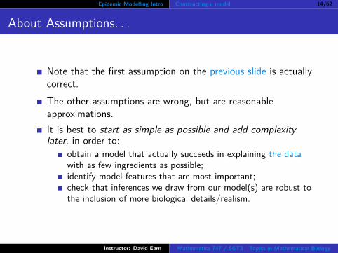
About Assumptions. . .
Note that the first assumption on the previous slide is actuallycorrect.The other assumptions are wrong, but are reasonableapproximations.It is best to start as simple as possible and add complexitylater, in order to:
obtain a model that actually succeeds in explaining the datawith as few ingredients as possible;identify model features that are most important;check that inferences we draw from our model(s) are robust tothe inclusion of more biological details/realism.
Instructor: David Earn Mathematics 747 / 5GT3 Topics in Mathematical Biology
Epidemic Modelling Intro Constructing a model 15/62
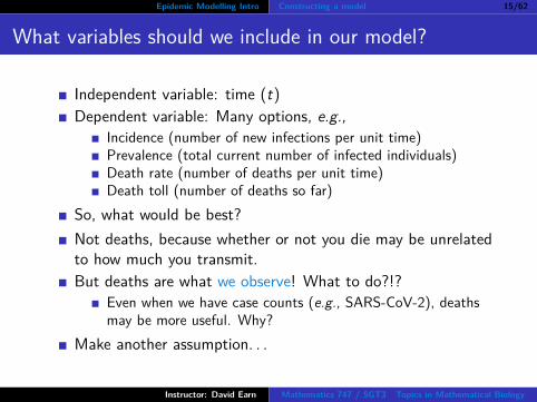
What variables should we include in our model?
Independent variable: time (t)Dependent variable: Many options, e.g.,
Incidence (number of new infections per unit time)Prevalence (total current number of infected individuals)Death rate (number of deaths per unit time)Death toll (number of deaths so far)
So, what would be best?Not deaths, because whether or not you die may be unrelatedto how much you transmit.But deaths are what we observe! What to do?!?
Even when we have case counts (e.g., SARS-CoV-2), deathsmay be more useful. Why?
Make another assumption. . .
Instructor: David Earn Mathematics 747 / 5GT3 Topics in Mathematical Biology

Epidemic Modelling Intro Constructing a model 16/62
Additional assumption(s)
We actually want to know incidence or prevalence, but weobserve deaths.Under what circumstances would daily deaths be a goodestimate of incidence? (i.e., What must we assume in additionto the assumptions we have already made.)
5 Assume that the time from infection to death is exactly thesame (a certain number of days) for every individual who dies.
6 Assume that the probability of dying from the disease is thesame for every individual who is infected.
Then daily death counts are proportional to daily incidence acertain number of days in the past, i.e., the “mortality curve”that we observe is a translated and scaled version of the“epidemic curve” (new cases per day).
Instructor: David Earn Mathematics 747 / 5GT3 Topics in Mathematical Biology

Epidemic Modelling Intro Constructing a model (cont.) 17/62
So. . . what variables should we include in our model?
Independent variable: time (t)Dependent variable: one of:
Incidence (number of new infections per unit time)Prevalence (total current number of infected individuals)
Which one?Choose prevalence (I) because anybody who is currentlyinfectious can infect others, so it will probably be easier toformulate a transmission model based on prevalence.(Try not to lose sight of underlying biological mechanisms.)But our mortality curve is related to incidence, notprevalence!?! Argh. What to do?!?Let’s work with prevalence and see how it works out.Maybe we’ll be able to derive the incidence curve from amodel based on prevalence.
Instructor: David Earn Mathematics 747 / 5GT3 Topics in Mathematical Biology

Epidemic Modelling Intro Constructing a model (cont.) 18/62
Notational note
We use I for prevalence because prevalence is the number ofinfected individuals.
So, let’s try to write down a model. . .
Instructor: David Earn Mathematics 747 / 5GT3 Topics in Mathematical Biology

Epidemic Modelling Intro Constructing a model (cont.) 19/62
A first (naıve) attempt at an epidemic model
Variables: time t, prevalence I(t)How does I increase?Start with I0 infected individuals at time t = 0. Whathappens for t > 0.Let B = average number of contacts with susceptibleindividuals that lead to a new infective per unit time perinfective in the population (and suppose B is constant). Then
I(t + ∆t) ' I(t) + B I(t)∆t
In the limit ∆t → 0, we have
dIdt = BI =⇒ I(t) = I0eBt
Instructor: David Earn Mathematics 747 / 5GT3 Topics in Mathematical Biology
Epidemic Modelling Intro Constructing a model (cont.) 20/62
Beware: implicit assumptions that should be explicit
Ignored discrete nature of individuals when taking limit.
Ignored finite infectious periods!
Sometimes it isn’t obvious that we’ve made some assumptionsuntil after we see what the model predicts.
Instructor: David Earn Mathematics 747 / 5GT3 Topics in Mathematical Biology
Epidemic Modelling Intro Constructing a model (cont.) 21/62
How can we tell if our model is good?
Compare model predictions with data.
What is the best way to do that?
Depends on what predictions we’re trying to test.
Model predicts exponential growth.How should we test that prediction?
Transforming the data might help.
Instructor: David Earn Mathematics 747 / 5GT3 Topics in Mathematical Biology
Epidemic Modelling Intro Constructing a model (cont.) 22/62
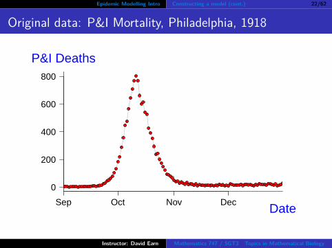
Original data: P&I Mortality, Philadelphia, 1918
Sep Oct Nov Dec
0
200
400
600
800
P&I Deaths
Date
Instructor: David Earn Mathematics 747 / 5GT3 Topics in Mathematical Biology
Epidemic Modelling Intro Constructing a model (cont.) 23/62
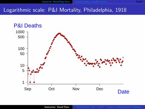
Logarithmic scale: P&I Mortality, Philadelphia, 1918
Sep Oct Nov Dec
1
510
50100
5001000
P&I Deaths
Date
Instructor: David Earn Mathematics 747 / 5GT3 Topics in Mathematical Biology

Epidemic Modelling Intro Constructing a model (cont.) 24/62
Parameter estimation
How can we estimate the model parameters, I0 and B, from theP&I data?
Fit a straight line through the part of the logarithmicmortality curve that looks straight.
The slope of the line is B.
The “intercept” is log I0.“Intercept” in quotes because we need to define t = 0 as thetime when exponential growth begins.
Note: Parameter estimation is, in general, a very trickybusiness and deserves a great deal of attention (beyond thescope of this course).
Instructor: David Earn Mathematics 747 / 5GT3 Topics in Mathematical Biology
Epidemic Modelling Intro Constructing a model (cont.) 25/62
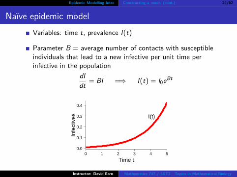
Naıve epidemic modelVariables: time t, prevalence I(t)
Parameter B = average number of contacts with susceptibleindividuals that lead to a new infective per unit time perinfective in the population
dIdt = BI =⇒ I(t) = I0eBt
0 1 2 3 4 50.0
0.1
0.2
0.3
0.4
Time t
Infe
ctiv
es I(t)
Instructor: David Earn Mathematics 747 / 5GT3 Topics in Mathematical Biology

Epidemic Modelling Intro Constructing a model (cont.) 26/62
Naıve model: the good and the bad
Good:Makes clear predictionsPredictions can be testedEstimation of parameter (B) is easy
B is the slope of the straight portion of the epidemic curve onthe log scale. (Why?)Remember we are imagining that the mortality curve isequivalent to the epidemic curve after translation and scaling.
Bad:Model is consistent only with exponential growth phase.Absurd long-term prediction: unbounded growth in I(t)
Implicitly assumed that population size N = ∞.
Instructor: David Earn Mathematics 747 / 5GT3 Topics in Mathematical Biology

Epidemic Modelling Intro Constructing a model (cont.) 27/62
How can we improve our model?
Insist that population size is finite (N <∞).
Keep track of both infectives I(t) and susceptibles S(t).
Assume individuals who are not infected are susceptible:
I(t) + S(t) = N = constant.
Instructor: David Earn Mathematics 747 / 5GT3 Topics in Mathematical Biology

Epidemic Modelling Intro Constructing a model (cont.) 28/62
New model parameter(s)?
B = average number of contacts with susceptible individualsthat lead to a new infective per unit time per infectiveIn the naıve model, we assumed B = constant.Is B really constant?B depends on how many susceptibles there are.B = βS(t)β = average number of contacts between susceptibles andinfectives that lead to a new infective
per unit timeper infectiveper susceptible
β is called the transmission rate.
Instructor: David Earn Mathematics 747 / 5GT3 Topics in Mathematical Biology

Epidemic Modelling Intro Constructing a model (cont.) 29/62
Revised epidemic model: “SI model”
dIdt = βS(t)I(t)
Two state variables. One equation. Problem? No:
dSdt = −βS(t)I(t)
But S(t) = N − I(t) =⇒ I(t) is still the only variable:
dIdt = βI(N − I)
Is this a better model?What does it predict?
Instructor: David Earn Mathematics 747 / 5GT3 Topics in Mathematical Biology
Epidemic Modelling Intro Constructing a model (cont.) 30/62
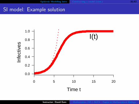
SI model: Example solution
0 5 10 15 20
0.0
0.2
0.4
0.6
0.8
1.0
Time t
Infe
ctiv
es
I(t)
Instructor: David Earn Mathematics 747 / 5GT3 Topics in Mathematical Biology

Epidemic Modelling Intro Constructing a model (cont.) 31/62
SI model: Analysis
We can find the exact solution. How?
I(t) = I0eNβt
1 + (I0/N)(eNβt − 1)But exact solution is not particularly enlightening.
Qualitative analysis:Initially I � N. What does the model predict then?Exponential growth. Great!As I grows, growth rate slows. Why?Fewer and fewer susceptibles to infect.Asymptotic behaviour? Equilibria? Periodic orbits?(periodic orbit = recurrent epidemics)(Non-trivial) periodic orbits impossible in one dimension(existence-uniqueness theorem).Consider equilibria. . .
Instructor: David Earn Mathematics 747 / 5GT3 Topics in Mathematical Biology
Epidemic Modelling Intro Constructing a model (cont.) 32/62
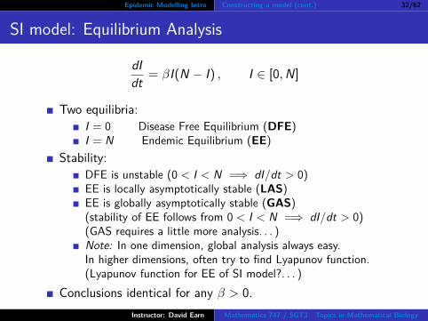
SI model: Equilibrium Analysis
dIdt = βI(N − I) , I ∈ [0,N]
Two equilibria:I = 0 Disease Free Equilibrium (DFE)I = N Endemic Equilibrium (EE)
Stability:DFE is unstable (0 < I < N =⇒ dI/dt > 0)EE is locally asymptotically stable (LAS)EE is globally asymptotically stable (GAS)(stability of EE follows from 0 < I < N =⇒ dI/dt > 0)(GAS requires a little more analysis. . . )Note: In one dimension, global analysis always easy.In higher dimensions, often try to find Lyapunov function.(Lyapunov function for EE of SI model?. . . )
Conclusions identical for any β > 0.Instructor: David Earn Mathematics 747 / 5GT3 Topics in Mathematical Biology
Epidemic Modelling Intro Constructing a model (cont.) 33/62
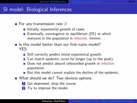
SI model: Biological Inferences
For any transmission rate β:Initially, exponential growth of cases.Eventually, convergence to equilibrium (EE) at whicheveryone in the population is infective. hmmm. . .
Is this model better than our first naıve model?YES.
Still correctly predict initial exponential growth.Can match epidemic curve for longer (up to the peak).Does not predict absurd unbounded growth in infectivepopulation.But this model cannot explain the decline of the epidemic.
What should we do? Two obvious options:1 Get depressed, drop the course.2 Try to improve the model.
Instructor: David Earn Mathematics 747 / 5GT3 Topics in Mathematical Biology

Epidemic Modelling Intro Recall the motivating data 34/62
Recall motivating data: 1918 flu in Philadelphia
Mortality curve (linear scale)
Mortality curve (log scale)
Instructor: David Earn Mathematics 747 / 5GT3 Topics in Mathematical Biology
Epidemic Modelling Intro Constructing a model (cont.) 35/62
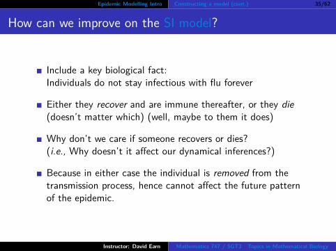
How can we improve on the SI model?
Include a key biological fact:Individuals do not stay infectious with flu forever
Either they recover and are immune thereafter, or they die(doesn’t matter which) (well, maybe to them it does)
Why don’t we care if someone recovers or dies?(i.e., Why doesn’t it affect our dynamical inferences?)
Because in either case the individual is removed from thetransmission process, hence cannot affect the future patternof the epidemic.
Instructor: David Earn Mathematics 747 / 5GT3 Topics in Mathematical Biology

Epidemic Modelling Intro The SIR model: Development 36/62
The SIR modelIntroduce new class of removed individuals:
R(t) = number of individuals who have either recovered andare now immune or have diedLet γ = rate of removal from the infective class (via recoveryor death)
dSdt = −βSI
dIdt = βSI − γI
dRdt = γI
Note: dSdt + dI
dt + dRdt = 0 =⇒ S + I + R = N = constant
Convenient to rescale variables by N and interpret S, I,R asproportions of the population in each disease state.
Instructor: David Earn Mathematics 747 / 5GT3 Topics in Mathematical Biology

Epidemic Modelling Intro The SIR model: Development 37/62
The SIR model: Example numerical solution
0 2 4 6 8
0.0
0.1
0.2
0.3
0.4
TimeCPU time: 0.16S, Vector field evaluations: 1944, Ratio: 12150
Proportion infected I(t)
β = 4γ = 1
Looks promising. . .
Instructor: David Earn Mathematics 747 / 5GT3 Topics in Mathematical Biology
Epidemic Modelling Intro The SIR model: Development 38/62
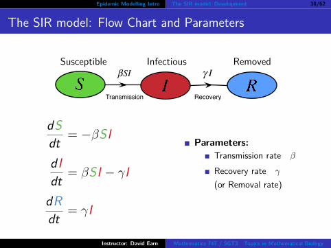
The SIR model: Flow Chart and Parameters
Susceptible Infectious Removed
Transmission Recovery
βSI γ I
dSdt = −βSI
dIdt = βSI − γI
dRdt = γI
Parameters:Transmission rate β
Recovery rate γ
(or Removal rate)
Instructor: David Earn Mathematics 747 / 5GT3 Topics in Mathematical Biology
Epidemic Modelling Intro The SIR model: Development 39/62
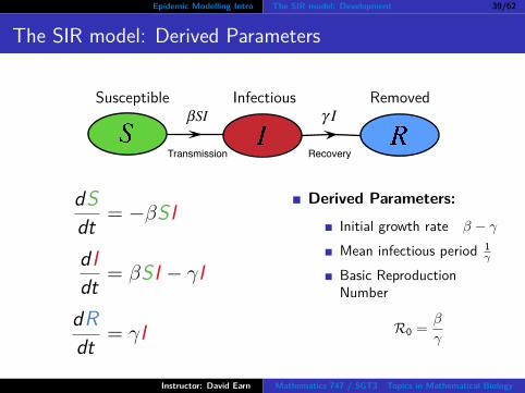
The SIR model: Derived Parameters
Susceptible Infectious Removed
Transmission Recovery
βSI γ I
dSdt = −βSI
dIdt = βSI − γI
dRdt = γI
Derived Parameters:
Initial growth rate β − γMean infectious period 1
γ
Basic ReproductionNumber
R0 = β
γ
Instructor: David Earn Mathematics 747 / 5GT3 Topics in Mathematical Biology
Epidemic Modelling Intro The SIR model: Development 40/62
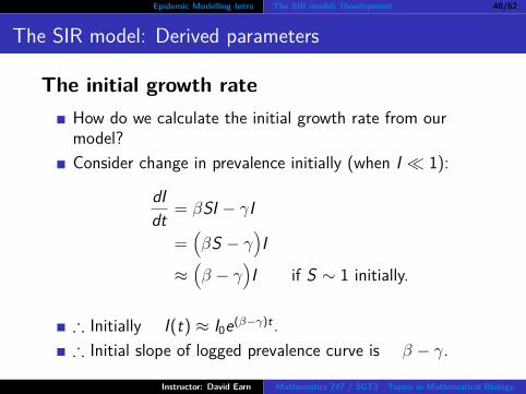
The SIR model: Derived parameters
The initial growth rateHow do we calculate the initial growth rate from ourmodel?Consider change in prevalence initially (when I � 1):
dIdt = βSI − γI
=(βS − γ
)I
≈(β − γ
)I if S ∼ 1 initially.
∴ Initially I(t) ≈ I0e(β−γ)t .∴ Initial slope of logged prevalence curve is β − γ.
Instructor: David Earn Mathematics 747 / 5GT3 Topics in Mathematical Biology
Epidemic Modelling Intro The SIR model: Development 41/62
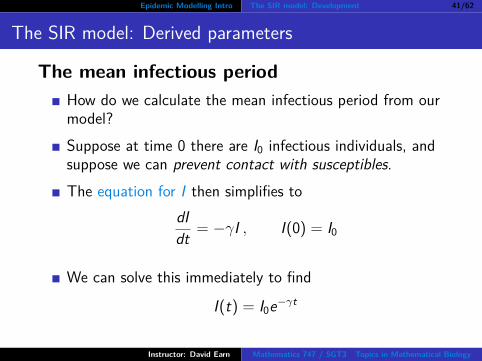
The SIR model: Derived parameters
The mean infectious periodHow do we calculate the mean infectious period from ourmodel?Suppose at time 0 there are I0 infectious individuals, andsuppose we can prevent contact with susceptibles.The equation for I then simplifies to
dIdt = −γI , I(0) = I0
We can solve this immediately to find
I(t) = I0e−γt
Instructor: David Earn Mathematics 747 / 5GT3 Topics in Mathematical Biology
Epidemic Modelling Intro The SIR model: Development 42/62
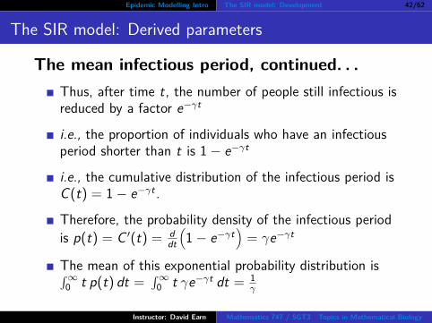
The SIR model: Derived parameters
The mean infectious period, continued. . .Thus, after time t, the number of people still infectious isreduced by a factor e−γt
i.e., the proportion of individuals who have an infectiousperiod shorter than t is 1− e−γt
i.e., the cumulative distribution of the infectious period isC(t) = 1− e−γt .
Therefore, the probability density of the infectious periodis p(t) = C ′(t) = d
dt
(1− e−γt
)= γe−γt
The mean of this exponential probability distribution is∫∞0 t p(t) dt =
∫∞0 t γe−γt dt = 1
γ
Instructor: David Earn Mathematics 747 / 5GT3 Topics in Mathematical Biology

Epidemic Modelling Intro The SIR model: Development 43/62
The SIR model: Derived parameters
The basic reproduction number R0
R0 = β · 1γ
= (transmission rate)× (mean infectious period)
R0 is dimensionless
R0 is the average number of secondary cases caused by aprimary case (in a wholly susceptible population).
We must have R0 > 1 to have an epidemic. Why?dIdt = βSI − γI =
(R0S − 1
)γI
∴ R0 ≤ 1 =⇒ dIdt ≤ 0 for all (S, I) ∈ [0, 1]2 =⇒ no growth
Instructor: David Earn Mathematics 747 / 5GT3 Topics in Mathematical Biology

Epidemic Modelling Intro The SIR model: Analysis 44/62
The SIR model: Analysis (biological well-posedness)
dSdt = −βSI
dIdt = βSI − γI
Be careful:Is this a sensiblebiologicalmodel?
We need S, I and R all non-negativeat all times.
Does 0 ≤ S(0) + I(0) ≤ 1 imply0 ≤ S(t) + I(t) ≤ 1 for all t > 0?
S = 0 =⇒ S ′ = 0, soS(0) ≥ 0 =⇒ S(t) ≥ 0 ∀t > 0.
I = 0 =⇒ I ′ = 0, soI(0) ≥ 0 =⇒ I(t) ≥ 0 ∀t > 0.
(S + I)′ = S ′ + I ′ = −γI ≤ 0=⇒ S + I is always non-increasing=⇒ S(t) + I(t) ≤ S(0) + I(0) ≤ 1.
Instructor: David Earn Mathematics 747 / 5GT3 Topics in Mathematical Biology

Epidemic Modelling Intro The SIR model: Analysis (cont.) 45/62
The SIR model: Analysis (equilibria etc.)
dSdt = −βSI
dIdt = βSI − γI
Equilibria:(S, I) = (S0, 0) forany S0 ∈ [0, 1]
Continuum ofequilibria.Does thismake sense?Biologicalmeaning ofequilibria?
Linearization:DF(S,I) =
(−βI −βSβI βS − γ
)
DF(S0,0) =(
0 −βS00 βS0 − γ
)All equilibria are non-hyperbolic.
Periodic orbits:(S + I)′ = −γI=⇒ no periodic orbits. Why?
If I(0) = 0 then equilibrium.If I(0) > 0 then (S + I)′ < 0, socannot increase back to initialstate.
Also follows from Index Theorem(cannot enclose any equilibria).
Instructor: David Earn Mathematics 747 / 5GT3 Topics in Mathematical Biology

Epidemic Modelling Intro The SIR model: Analysis (cont.) 46/62
Recap what we’ve done so far. . .
Began analysis of standard SIR model.
Showed SIR model:is biologically well-posedhas a continuum of (disease-free) equilibria, all of which arenon-hyperbolicdoes not have any periodic solutions
Instructor: David Earn Mathematics 747 / 5GT3 Topics in Mathematical Biology

Epidemic Modelling Intro The SIR model: Analysis (cont.) 47/62
The SIR model: Analysis
dSdt = −βSI
dIdt = βSI − γI
Nullclines:
S ′ = 0 =⇒ S = 0 or I = 0S nullclines: both coordinate axes
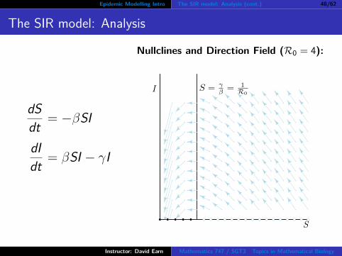
I ′ = 0 =⇒ I = 0 or S = γ/β
I nullclines: S axis and vertical lineat S = 1/R0
Is the I nullcline at S = 1/R0 alwaysrelevant?
If, and only if, R0 > 1.If R0 < 1 then S = 1/R0 isoutside the biologically relevantregion of the (S, I) phase plane.
Instructor: David Earn Mathematics 747 / 5GT3 Topics in Mathematical Biology
Epidemic Modelling Intro The SIR model: Analysis (cont.) 48/62
The SIR model: Analysis
dSdt = −βSI
dIdt = βSI − γI
Nullclines and Direction Field (R0 = 4):
S
I S = γβ = 1
R0
Instructor: David Earn Mathematics 747 / 5GT3 Topics in Mathematical Biology

Epidemic Modelling Intro The SIR model: Analysis (cont.) 49/62
The SIR model: Analysis
dSdt = −βSI
dIdt = βSI − γI
Phase Portrait:We cannot findsolutions S(t) andI(t) for this system.We can find exactanalytical solution forthe phase portrait!
i.e., we can find an expression I(S) forsolution curves in the (S, I) phase plane.Slope of I(S) depends only on S:
dIdS = dI/dt
dS/dt = − 1 + 1R0S (∗)
Note: Slope is flat for S = 1/R0, so maxor min of I(S) occurs on I nullcline ifR0 > 1Easy to integrate (∗):∫ I
I0 dI =∫ S
S0
(−1 + 1
R0S
)dS
I − I0 = −(S − S0) + 1R0
log (S/S0)
Instructor: David Earn Mathematics 747 / 5GT3 Topics in Mathematical Biology

Epidemic Modelling Intro The SIR model: Analysis (cont.) 50/62
The SIR model: Analysis
Model Equations:
dSdt = −βSI
dIdt = βSI − γI
Solution Curves inPhase Plane:
I + S − (I0 + S0)
= 1R0
log (S/S0)
Phase Portrait (R0 = 4):
S
I S = γβ = 1
R0
Instructor: David Earn Mathematics 747 / 5GT3 Topics in Mathematical Biology

Epidemic Modelling Intro The SIR model: Analysis (cont.) 51/62
The SIR model: Analysis
Model Equations:
dSdt = −βSI
dIdt = βSI − γI
Solution Curves inPhase Plane:
I + S − (I0 + S0)
= 1R0
log (S/S0)
Final Size of Epidemic:As t →∞ we have(I∞ + S∞)− (I0 + S0) = 1
R0log S∞/S0
But for a newly invading pathogen:S0 ' 1, I0 ' 0, I∞ = 0In the limit I0 → 0, we have(S∞ − 1) = 1
R0log S∞
Define “Final Size” Z = 1− S∞∴ −Z = 1
R0log (1− Z ), i.e.,
Z = 1− e−R0Z
This is a famous formula, derived byKermack and McKendrick in 1927.
Instructor: David Earn Mathematics 747 / 5GT3 Topics in Mathematical Biology

Epidemic Modelling Intro The SIR model: Analysis (cont.) 52/62
The SIR model: Analysis
Final Size Formula:
Z = 1− e−R0Z
Final size isdetermined entirelyby R0
Final size is never thewhole population(Z < 1)Formula is valid formuch more realisticmodels (Ma & Earn,2006)
0 2 4 6 8 100.0
0.2
0.4
0.6
0.8
1.0
Fin
al S
ize
approxexact
Basic Reproduction Number R0
For 1918 flu: 1.5 . R0 . 2Proportion of world populationinfected?∼ 60–80%
Instructor: David Earn Mathematics 747 / 5GT3 Topics in Mathematical Biology
Epidemic Modelling Intro The SIR model: Analysis (cont.) 53/62
From Final Size to Reproduction Number
The final size relation allows us to estimate the proportion ofthe population that will be infected given an estimate of R0.
But we can turn it around: if we know the final size Z thenwe can easily estimate R0:
Z = 1− e−R0Z =⇒ R0 = − 1Z log (1− Z )
This is useful post-hoc only (after an epidemic).
Instructor: David Earn Mathematics 747 / 5GT3 Topics in Mathematical Biology

Epidemic Modelling Intro The SIR model: Analysis (cont.) 54/62
The SIR model: Non-dimensionalization
Often helpful to use dimensionless parameters.How do we identify “the right” dimensionless parameters?βγ ? γ
β ? ββ+γ ? β2
β2+γ2 ?We choose β/γ because it has a natural interpretation.But we are still left with γ as a second parameter.Can we simplify the model somehow?γ defines a time scale (1/γ is the mean infectious period).If time unit is mean infectious period, then γ = 1.So in these “natural” time units, the SIR model is
dSdt = −R0SI, dI
dt = R0SI − I
There is really only one parameter in the model. The other isjust a time scale and does not affect the qualitative dynamics.
Instructor: David Earn Mathematics 747 / 5GT3 Topics in Mathematical Biology
Epidemic Modelling Intro Taking stock 55/62
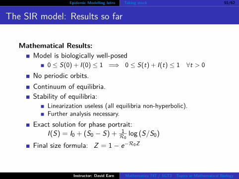
The SIR model: Results so far
Mathematical Results:Model is biologically well-posed
0 ≤ S(0) + I(0) ≤ 1 =⇒ 0 ≤ S(t) + I(t) ≤ 1 ∀t > 0No periodic orbits.Continuum of equilibria.Stability of equilibria:
Linearization useless (all equilibria non-hyperbolic).Further analysis necessary.
Exact solution for phase portrait:I(S) = I0 + (S0 − S) + 1
R0log (S/S0)
Final size formula: Z = 1− e−R0Z
Instructor: David Earn Mathematics 747 / 5GT3 Topics in Mathematical Biology

Epidemic Modelling Intro Stability 56/62
The SIR model: Stability of equilibria
Phase Portrait (R0 = 4):
S
I S = γβ = 1
R0
Model Equations:
dSdt = −βSI, dI
dt = βSI − γI
Which equilibria are:Unstable?
S0 > 1/R0
Stable?S0 ≤ 1/R0
Asymptotically stable?None!
How do we prove thesefacts?
Instructor: David Earn Mathematics 747 / 5GT3 Topics in Mathematical Biology

Epidemic Modelling Intro Control measures 57/62
The SIR model: Effects of Control Measures
How could the final size of the 1918 pandemic have beenreduced?
Any intervention that reduces R0 reduces the final size.
What could have been done to reduce R0?
Masks? Quarantine? Isolation?
Ideally a vaccine, but no such luck in 1918.
Even in 2009, it took months to mass-produce vaccine.
But suppose there had been a vaccine immediately. . .
What proportion (p) of the population do we need tovaccinate to eradicate an infectious disease?
Instructor: David Earn Mathematics 747 / 5GT3 Topics in Mathematical Biology

Epidemic Modelling Intro Control measures 58/62
The SIR model: Effects of Control MeasuresSuppose a proportion (p) of the population is vaccinated before anepidemic starts. Then:
At the start of the epidemic, the proportion of the populationthat is susceptible is S0 = 1− p.∴ Initially (at time t = 0) the rate of change of prevalence is
dIdt
∣∣∣∣t=0
=((R0S − 1
)I)∣∣∣
t=0=(R0S0 − 1
)I0
=(R0(1− p)− 1
)I0 < 0 ⇐⇒ R0(1− p) < 1
∴ An epidemic will be prevented if
p > pcrit = 1− 1R0
∴ Public Health Agency will ask you to estimate R0.Instructor: David Earn Mathematics 747 / 5GT3 Topics in Mathematical Biology
Epidemic Modelling Intro Taking stock 59/62
The SIR model: Results so far
Biological inferences:
R0 is extremely important to estimate in practice!
Epidemic occurs if and only if R0 > 1.
Single epidemic, then disease disappears.
Can prevent epidemic by vaccinating (or otherwise removing)a proportion 1− 1
R0from the transmission process.
Note: It doesn’t matter whether we remove people from the susceptible pool byvaccination, isolation, or other means. What matters is the proportion of the
population who are removed from the transmission process.
Instructor: David Earn Mathematics 747 / 5GT3 Topics in Mathematical Biology

Epidemic Modelling Intro Taking stock 60/62
The SIR model: Does it explain our data?
What about 1918 flu in Philadelphia?
Sep Oct Nov Dec
0
200
400
600
800
P&I Deaths
Date
Does the SIR model explain these data?Can we fit the SIR model to the P&I time series?If so, are our estimated parameter values (for R0 and 1/γ)biologically reasonable?
Instructor: David Earn Mathematics 747 / 5GT3 Topics in Mathematical Biology

Epidemic Modelling Intro Taking stock 61/62
The SIR model: How solutions depend on R0
0 2 4 6 8
0.0
0.1
0.2
0.3
0.4
Time [mean infectious periods]CPU time: 0.067S, Vector field evaluations: 1944, Ratio: 29014.9
R0
432.5
Proportion infected I(t)
Instructor: David Earn Mathematics 747 / 5GT3 Topics in Mathematical Biology

Epidemic Modelling Intro Renewal Equation 62/62
The SIR model: prevalence vs. incidenceIn the SIR model as we have defined it, prevalence is I(t) andincidence is i(t) = βS(t)I(t) ,so we can compute incidence i(t) from solutions to the SIR model,and then compare predicted incidence with observed reports of casesor deaths.Could we have derived an equally sensible model starting from thecloser-to-observable quantity (incidence i) ?The answer is YES,
dSdt = −i(t) , (1a)
i(t) = R0 S(t)∫ ∞
0i(t − s) g(s) ds , (1b)
where g(s) is the generation interval distribution.How do solutions of this integro-differential equation differ fromthose of the SIR model as we have defined it?
If you are curious, see Champredon, Dushoff & Earn 2018.
Instructor: David Earn Mathematics 747 / 5GT3 Topics in Mathematical Biology