EpiData Introduction Guide A Canadian Example

Created as part of a collaborative project1 : Association of Public Health Epidemiologists in Ontario (APHEO), the EpiData Association and the Public Health Agency of Canada. Authors: APHEO EpiData Expert Panel and J.Lauritsen, EpiData Association.

V6.0 Jan 2011

1 This project has been made possible through a financial contribution from the Public Health Agency of Canada

2

Table of Contents Purpose and scope........................................................................................................................... 3

Introduction - Background of Outbreak.......................................................................................... 3

Introduction – EpiData Entry and Analysis Software..................................................................... 3

Preparation ...................................................................................................................................... 4

A. Read about data management and structures ......................................................................... 4

B. Acquire and install software................................................................................................... 4

C. Starting a New Project............................................................................................................ 6

PART 1: EpiData Entry .................................................................................................................. 7

Planning the Questionnaire ......................................................................................................... 7

Create the Questionnaire............................................................................................................. 7

Create the Data File .................................................................................................................... 8

Enter Data in the Questionnaire.................................................................................................. 9

Specifying Data Entry Rules/Checks.......................................................................................... 9

PART 2: EpiData Analysis ........................................................................................................... 14

Opening and preparing the dataset............................................................................................ 14

Fine tuning the dataset for analysis (data cleaning).................................................................. 17

Descriptive Epidemiology ........................................................................................................ 18

Creating an Epidemic Curve................................................................................................. 19

Analytical Epidemiology .......................................................................................................... 23

Food Specific Attack Rate Table .......................................................................................... 23

Stratified Analysis using CIplot............................................................................................ 26

PART 3: Working with programs................................................................................................. 27

PART 4: Extensions to the exercises ............................................................................................ 29

Questions/For More Information .................................................................................................. 30

Appendix 1 - Importing Date/Time Fields from Excel................................................................. 31

3

Purpose and scope

This introductory text is created for self-instruction or a short facilitated seminar of 3 to 4 hours in length. Actual length depends on the number of facilitators and the audience’s experience with EpiData. Participants should have prior understanding of outbreak investigation methods and the associated statistical methods. The structure of this guide includes the principles of defining and entering data followed by basic analysis principles for a simplified dataset, and finally in part three, follow-up exercises for the experienced user or a follow-up seminar. Part three would normally not be part of the first 3 to 4 hour seminar. Data used herein are partially modified for exercise purposes and cannot be published except by written permission.

This instruction is based on the study “Bridal Shower Outbreak” By York Region Community and Health Services, Ontario, Canada

Introduction - Background of Outbreak An outbreak of gastrointestinal illness was declared by York Region Community and Health Services on February 26, 2008, following a bridal shower held at a banquet hall on February 24, 2008. Approximately 75 guests were served meals, and 36 employees worked as food handlers as part of this event. Food history questionnaires were administered to 48 symptomatic and 16 asymptomatic persons. EpiData Entry was used to create the questionnaire form and the data was then entered.

A retrospective cohort design was used to collect and analyze the data. A retrospective cohort study relies on historical exposure data. In this outbreak, a representative sample of participants was interviewed, allowing the comparison of the rate of disease in those who did or did not eat a certain food. This type of study is the technique of choice when one is faced with an acute outbreak in a well-defined population.

Introduction – EpiData Entry and Analysis Software EpiData is a free software suite designed to assist epidemiologists, public health investigators and others to enter, manage and analyze data in the field. All software is available from http://www.epidata.dk . A number of field guides, software documentation notes, examples and other information are also available. Users are encouraged to: (1) Join the EpiData-list discussion group, and (2) Sign up for the information newsletters sent periodically each year. To subscribe to the discussion group and sign up for the newsletters, visit the EpiData website at http://www.epidata.dk

4

Preparation Follow steps A, B and C:

A. Read about data management and structures

Go through the document: http://www.epidata.org/wiki/index.php/Field_guide:_from_question_to_data which discusses data structures, data management and documentation.

B. Acquire and install software

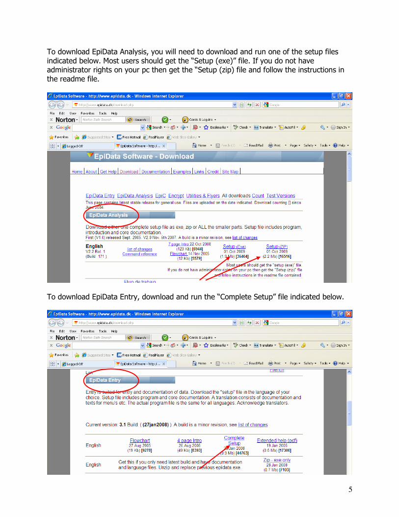
Download EpiData Analysis (v2.2 or later) and EpiData Entry (v3.1 or later) and install these on your computer. You should use the most recent version available from the download section of the website http://www.epidata.dk/download.php If installation on your computer requires the permission of an administrator, you can install the software into your private folder (create a subfolder on the desktop) or on a USB key2.

2It is also good practice to talk with the administrator. All EpiData Software is checked with up-to date anti-virus and other malicious software protection agents before uploading to epidata.dk.

5

To download EpiData Analysis, you will need to download and run one of the setup files indicated below. Most users should get the “Setup (exe)” file. If you do not have administrator rights on your pc then get the “Setup (zip) file and follow the instructions in the readme file.

To download EpiData Entry, download and run the “Complete Setup” file indicated below.

6

C. Starting a New Project

Create and name a new folder Create a project folder that will house all data files associated with your investigation – this folder can be located anywhere on your computer; you do not have to create one in the same drive as the EpiData program files. For the purposes of this exercise, create a new project folder on your desktop titled “BridalShower”. Get the necessary exercise data file from the Association of Public Health Epidemiologists in Ontario’s (APHEO) website (http://www.apheo.ca/index.php?pid=47#Project Documents), save the “Outbreak.zip” file to your computer (you can save it on your desktop or into a ‘temp’ folder in your c:\ drive) and UNZIP this file into your project folder. If you have no other unzip software, EpiData Entry has a utility in the main menu.

7

PART 1: EpiData Entry Before you create a questionnaire and enter data, the following steps must be considered: a. What is the purpose of the investigation? b. Organizational aspects. e.g. Will the investigation take place in one or several sites? c. What sampling design of observations is appropriate and which sources of information

can you use? (interview, registry data, laboratory data .....) d. Which data structure will enable us to do the investigation in view of sampling design,

purpose, organization and types of data sources?

Planning the Questionnaire

Determine its purpose: Is there an outbreak, and if so, is it related to certain food items?

Task 1: The first task is to define groups of information. Write down titles of types of information you would include, for example: Demographic factors, exposure, logistics, symptoms, diagnostics

Task 2: Formulate the questions you want to include. A simple first version of a data

structure could be: age, sex, public health unit, symptomsi, date of onset, fooditemsj where i and j indicate several of these.

Create the Questionnaire

Task 3: Now define the actual data structure. First: Start EpiData Entry and

open the introduction pdf file by clicking on the Help button and selecting “Introduction to EpiData” in the droplist. Read this document beforehand.

8

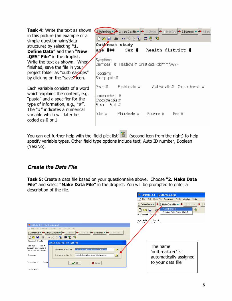
Task 4: Write the text as shown

in this picture (an example of a simple questionnaire/data structure) by selecting “1. Define Data” and then “New .QES” File” in the droplist. Write the text as shown. When finished, save the file in your project folder as “outbreak.qes” by clicking on the “save” icon. Each variable consists of a word which explains the content, e.g. “pasta” and a specifier for the type of information, e.g., “#”. The “#” indicates a numerical variable which will later be coded as 0 or 1. You can get further help with the ‘field pick list’ (second icon from the right) to help specify variable types. Other field type options include text, Auto ID number, Boolean (Yes/No).

Create the Data File

Task 5: Create a data file based on your questionnaire above. Choose “2. Make Data File” and select “Make Data File” in the droplist. You will be prompted to enter a description of the file.

The name ‘outbreak.rec’ is automatically assigned to your data file

9

What can go wrong here is that you have not saved your .qes file first, or that you chose “preview data form” instead of “create data file”.

Enter Data in the Questionnaire

Task 6: Entering data in your newly created questionnaire Close your outbreak.qes file (ensure it has been saved!). Choose “4. Enter Data” and select “outbreak.rec”. Enter five “made up” records and see if you can enter an illegal date, e.g. February 29th in a “non-leap” year in the “Onset date” field.

Task 7: Actual entry – how did it work? You should now have noticed that by just defining the onset date in the dd/mm/yyyy format, you already have sufficient control for not entering an illegal date. But in the other fields you could enter any number, whether it makes sense or not. Therefore, you must impose further controls.

Specifying Data Entry Rules/Checks

Task 8: Add checks/controls by selecting the “3. Checks” section A strong component of EpiData is the ability to specify rules during data entry. For example, you can design your questionnaire to:

• Restrict data entry to certain values and give text descriptions to the numerical codes entered. • Specify sequence of data entry, e.g. fill out certain questions for males only (i.e., build in question jumps). • Apply calculations during data entry, e.g. age at visit = date of visit - date of birth. Typically most calculations are done at the analysis stage.

10

Hint: Close data-entry (F10) and read the section on adding checks in the

Introduction to EpiData document.

Select the ‘outbreak.rec’ file. Your questionnaire will appear along with the ‘check’ window:

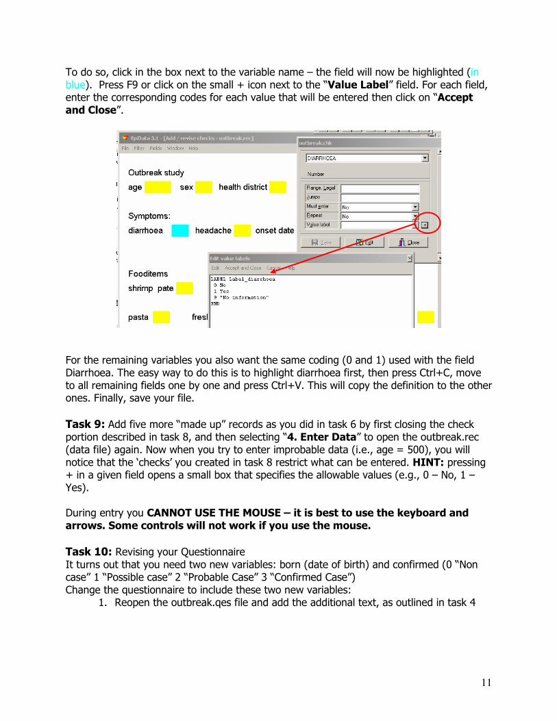
Earlier, you defined some of our data fields as numeric (#). Now, assign labels to the numeric values:

Diarrhoea 0 = No 1 = Yes

Sex 1 = Female 2 = Male

Health Unit

1 = York 2 = Peel 3 =Toronto

11

To do so, click in the box next to the variable name – the field will now be highlighted (in blue). Press F9 or click on the small + icon next to the “Value Label” field. For each field, enter the corresponding codes for each value that will be entered then click on “Accept and Close”.

For the remaining variables you also want the same coding (0 and 1) used with the field Diarrhoea. The easy way to do this is to highlight diarrhoea first, then press Ctrl+C, move to all remaining fields one by one and press Ctrl+V. This will copy the definition to the other ones. Finally, save your file.

Task 9: Add five more “made up” records as you did in task 6 by first closing the check portion described in task 8, and then selecting “4. Enter Data” to open the outbreak.rec (data file) again. Now when you try to enter improbable data (i.e., age = 500), you will notice that the ‘checks’ you created in task 8 restrict what can be entered. HINT: pressing + in a given field opens a small box that specifies the allowable values (e.g., 0 – No, 1 – Yes). During entry you CANNOT USE THE MOUSE – it is best to use the keyboard and arrows. Some controls will not work if you use the mouse.

Task 10: Revising your Questionnaire It turns out that you need two new variables: born (date of birth) and confirmed (0 “Non case” 1 “Possible case” 2 “Probable Case” 3 “Confirmed Case”) Change the questionnaire to include these two new variables:

1. Reopen the outbreak.qes file and add the additional text, as outlined in task 4

12

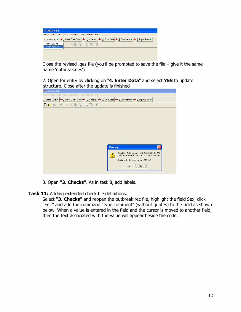
Close the revised .qes file (you’ll be prompted to save the file – give it the same name ‘outbreak.qes’) 2. Open for entry by clicking on “4. Enter Data” and select YES to update structure. Close after the update is finished

3. Open “3. Checks”. As in task 8, add labels.

Task 11: Adding extended check file definitions.

Select “3. Checks” and reopen the outbreak.rec file, highlight the field Sex, click “Edit” and add the command “type comment” (without quotes) to the field as shown below. When a value is entered in the field and the cursor is moved to another field, then the text associated with the value will appear beside the code.

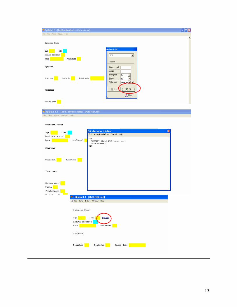
13

14

PART 2: EpiData Analysis EpiData Analysis is used to analyze EpiData *.rec files, dBase *.dbf files, and text *.csv files. The EpiData Analysis screen is easy to navigate and functionality is accessible via the use of shortcut keys. For the purposes of this field guide, areas of importance are: • The command prompt (F4) area located at the bottom of the screen

• The editor (F5) • The results window. • The dialogs in the work process toolbar. But also take some time to explore additional functionality available via other short cut keys. When you open EpiData Analysis, you see the following menu:

Opening and preparing the dataset

Note: when working with EpiData Analysis, the file that will be used is titled “EpiData example_rev2.dbf”. All files are available on the Association of Public Health Epidemiologists in Ontario’s website at http://www.apheo.ca/index.php?pid=47#Project Documents in the Outbreak.zip file. To open a data file, click on “Read”:

Navigate to the location where you saved your file (in your project folder) and select it.

Change Folder

Main menu

Work Process Toolbar

With dialogs

Statusbar

Command

Prompt (F4)

Results window

(Viewer)

Results

window

control

Editor(F5)

Browse

data (F6)

History

(F7)

Variables

(F3)

Commands

(F2)

Change Folder

Main menu

Work Process Toolbar

With dialogs

Statusbar

Command

Prompt (F4)

Results window

(Viewer)

Results

window

control

Editor(F5)

Browse

data (F6)

History

(F7)

Variables

(F3)

Commands

(F2)

15

EpiData will provide some information about the data: name, number of records number of fields, etc. In this case you have 64 records in the dataset.

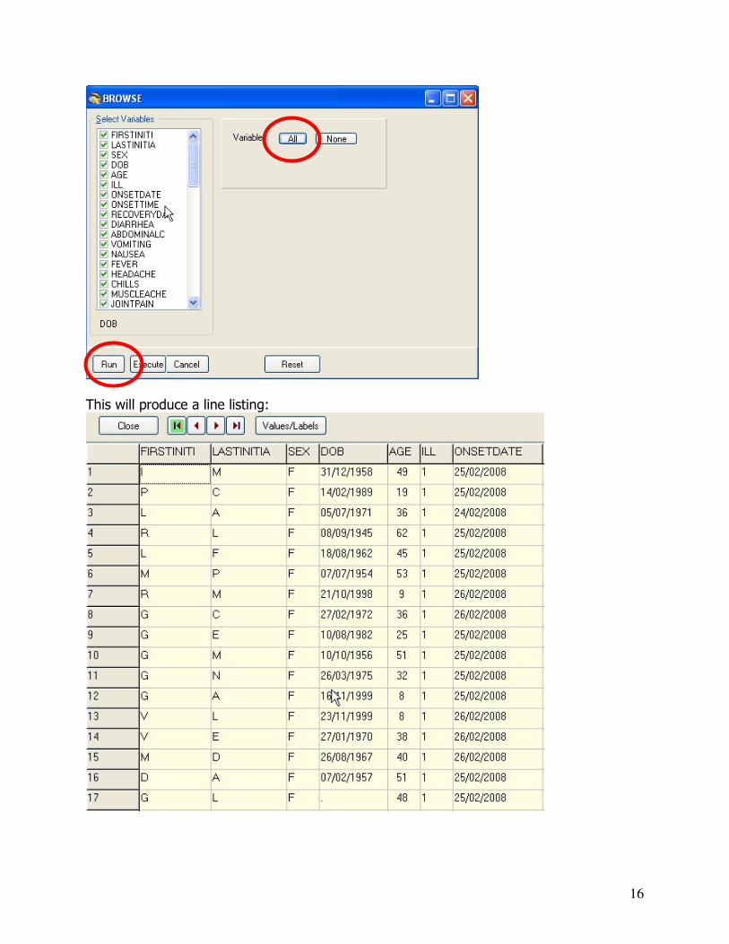
Press F2 to reveal all commands as well as F3 to display the file’s variables: Now take a look at the data by selecting “Browse”:

Click on the “All” button to select all available variables then click on the “Run” button.

16

This will produce a line listing:

17

Fine tuning the dataset for analysis (data cleaning)

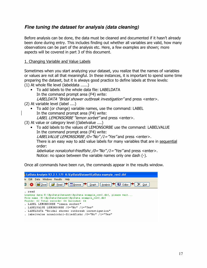
Before analysis can be done, the data must be cleaned and documented if it hasn’t already been done during entry. This includes finding out whether all variables are valid, how many observations can be part of the analysis etc. Here, a few examples are shown; more aspects will be covered in part 3 of this document. 1. Changing Variable and Value Labels Sometimes when you start analyzing your dataset, you realize that the names of variables or values are not all that meaningful. In these instances, it is important to spend some time preparing the dataset, but it is always good practice to define labels at three levels: (1) At whole file level (labeldata ......)

• To add labels to the whole data file: LABELDATA In the command prompt area (F4) write: LABELDATA “Bridal shower outbreak investigation” and press <enter>.

(2) At variable level (label ....) • To add (or change) variable names, use the command: LABEL

In the command prompt area (F4) write: LABEL LEMONSORBE “lemon sorbet” and press <enter>.

(3) At value or category level ((labelvalue ....)

• To add labels to the values of LEMONSORBE use the command: LABELVALUE In the command prompt area (F4) write: LABELVALUE LEMONSORBE /0=”No” /1=”Yes” and press <enter>. There is an easy way to add value labels for many variables that are in sequential order: labelvalue nonalcohol-friedfishc /0=”No” /1=”Yes” and press <enter>. Notice: no space between the variable names only one dash (-).

Once all commands have been run, the commands appear in the results window.

18

2. Creating New Variables and Adding Conditional Values During the data entry process, the age of each case and non-case was collected in two ways. Each was asked the birth date and the age at investigation. Now that you want to analyze the data, group ages into categories by creating a new variable called “agegrp”. For now you will only use the age at investigation (age), whereas calculation of age based on Date of Investigation and Date of Birth follows in part 3. You are going to use the “DEFINE” and "RECODE" commands.

In the command prompt (F4) area, write:

* create your age group variable as an integer: define agegrp # recode age to agegrp 0-9=1 10-19=2 20-44=3 45-64=4 65-hi=5

The command “recode” also adds the value label in the intervals indicated. You will see a new variable called agegrp in the variable list (F3). Note: Descriptive comments which appear in green can be added to your code using ‘*’ at the start of the sentence.

Descriptive Epidemiology

Describing the cases in terms of person, place and time is good epidemiological practice and can help you develop hypotheses about the mode of transmission and the source of infection. Let’s start with person: In order to know how many cases and non-cases you have, you can do a frequency distribution of the variable ILL. In the command prompt area (F4), write: Freq ill

You can see that there are 48 cases and 16 non-cases. • (Where 0=non-case and 1=case)

Now, analyze the demographic data to determine the age and sex structure of the population at risk. Use the new variable you just created above – agegrp. Once again, at the command prompt (F4), type: tables sex agegrp /c This will produce a cross tabulation of sex by age group along with column percents. Your table should look like this:

19

You can see that the majority of the population is between the ages of 20 and 64 years.. You can add row percents as well by adding /r to the end of the command line. If you did this, you would also see that more than 80% are women. Next, click on “Analysis”, then select “Describe” This command is used to provide a descriptive summary of the content of a continuous numeric field such as AGE:

For the variable AGE, the total number of records used in the calculation are given (N=64) as well as the sum, mean age, 95% confidence interval, the minimum value, percentiles (5, 10, 25, 50=Median, 75, 90 and 95) and the maximum value.

Creating an Epidemic Curve

Describing your cases with respect to time will give you clues to understanding the mode of transmission of the disease, the source and the nature of the etiologic agent (incubation period). An epidemic curve is a graph that provides a visual display of the magnitude and time course of an outbreak. The epidemic curve plots time along the X-axis and number of cases along the Y-axis. Because time is continuous, the epidemic curve is drawn as a histogram (no gaps between adjacent columns). Before creating the epicurve, select only those people that were ill – the non-cases are not contributing to analysis of date of onset.

20

In the command prompt (F4), write: Select ill=1 Notice how the status bar at the bottom changes with the select command.

Click on “Graph” and select “Epidemic Curve” from the droplist.

Now, create the epidemic curve based on the graph dialog for epidemic curves, which will formulate the command as: Epicurve ill onsetdate Select “Ill” as the Outcome variable and “OnsetDate” as the Time variable.

21

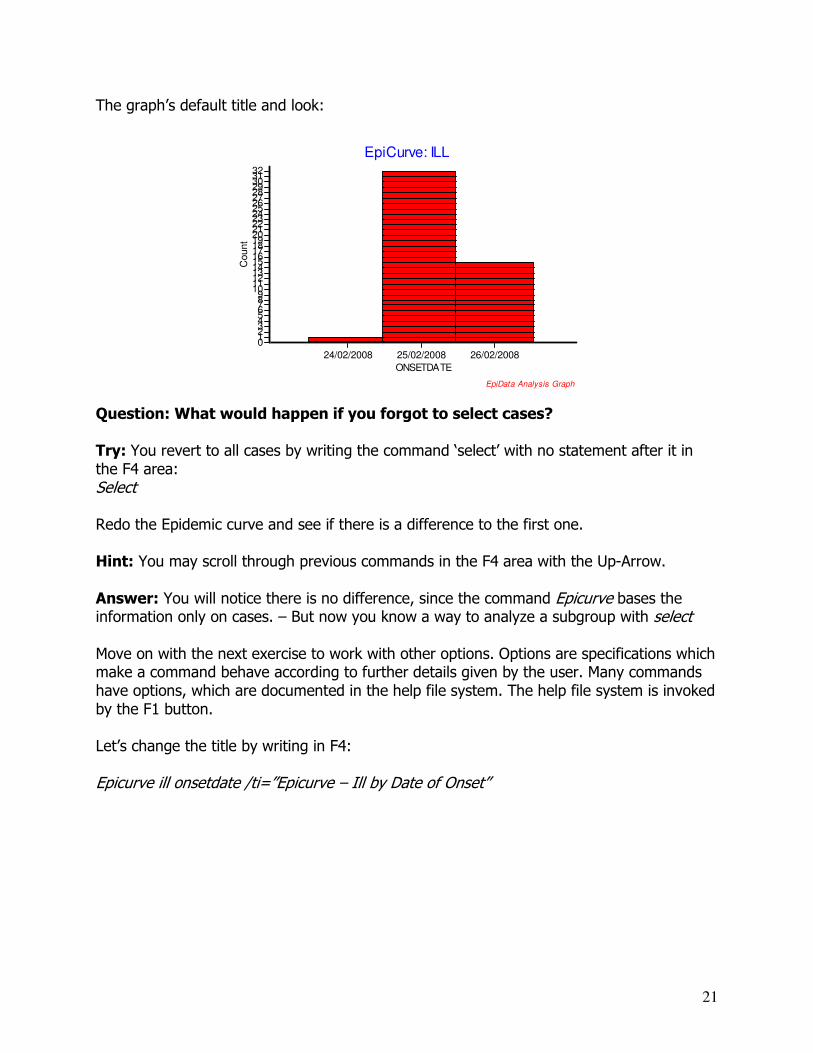
The graph’s default title and look:

EpiCurve: ILL

EpiData Analysis Graph

ONSETDATE

24/02/2008 25/02/2008 26/02/2008

Count

32313029282726252423222120191817161514131211109876543210

Question: What would happen if you forgot to select cases? Try: You revert to all cases by writing the command ‘select’ with no statement after it in the F4 area: Select Redo the Epidemic curve and see if there is a difference to the first one. Hint: You may scroll through previous commands in the F4 area with the Up-Arrow. Answer: You will notice there is no difference, since the command Epicurve bases the information only on cases. – But now you know a way to analyze a subgroup with select Move on with the next exercise to work with other options. Options are specifications which make a command behave according to further details given by the user. Many commands have options, which are documented in the help file system. The help file system is invoked by the F1 button. Let’s change the title by writing in F4: Epicurve ill onsetdate /ti=”Epicurve – Ill by Date of Onset”

22

Epicurve - Ill by Date of Onset

EpiData Analysis Graph

ONSETDATE

24/02/2008 25/02/2008 26/02/2008

Count

32313029282726252423222120191817161514131211109876543210

Now, change the y axis label: Epicurve ill onsetdate /ti=”Epicurve – Ill by Date of Onset” /ytext=”Number Ill”

Epicurve - Ill by Date of Onset

EpiData Analysis Graph

ONSETDATE

24/02/2008 25/02/2008 26/02/2008

Num

ber

Ill

32313029282726252423222120191817161514131211109876543210

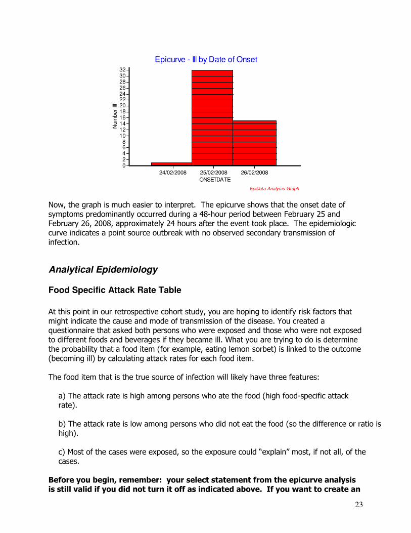
The y-axis numbers are tight. Change the increment to 2: Epicurve ill onsetdate /ti=”Epicurve – Ill by Date of Onset” /ytext=”Number Ill” /yinc=2

23

Epicurve - Ill by Date of Onset

EpiData Analysis Graph

ONSETDATE

24/02/2008 25/02/2008 26/02/2008

Num

ber

Ill

32302826242220181614121086420

Now, the graph is much easier to interpret. The epicurve shows that the onset date of symptoms predominantly occurred during a 48-hour period between February 25 and February 26, 2008, approximately 24 hours after the event took place. The epidemiologic curve indicates a point source outbreak with no observed secondary transmission of infection.

Analytical Epidemiology

Food Specific Attack Rate Table

At this point in our retrospective cohort study, you are hoping to identify risk factors that might indicate the cause and mode of transmission of the disease. You created a questionnaire that asked both persons who were exposed and those who were not exposed to different foods and beverages if they became ill. What you are trying to do is determine the probability that a food item (for example, eating lemon sorbet) is linked to the outcome (becoming ill) by calculating attack rates for each food item. The food item that is the true source of infection will likely have three features:

a) The attack rate is high among persons who ate the food (high food-specific attack rate).

b) The attack rate is low among persons who did not eat the food (so the difference or ratio is high).

c) Most of the cases were exposed, so the exposure could “explain” most, if not all, of the cases.

Before you begin, remember: your select statement from the epicurve analysis is still valid if you did not turn it off as indicated above. If you want to create an

24

attack rate table of ill/not ill by food consumed, you must remove your selection

(ill=1). This is easy to do. In your command prompt (F4), type ‘select’. Verify that the command is correct by typing: Freq ill Both ill/not ill should appear:

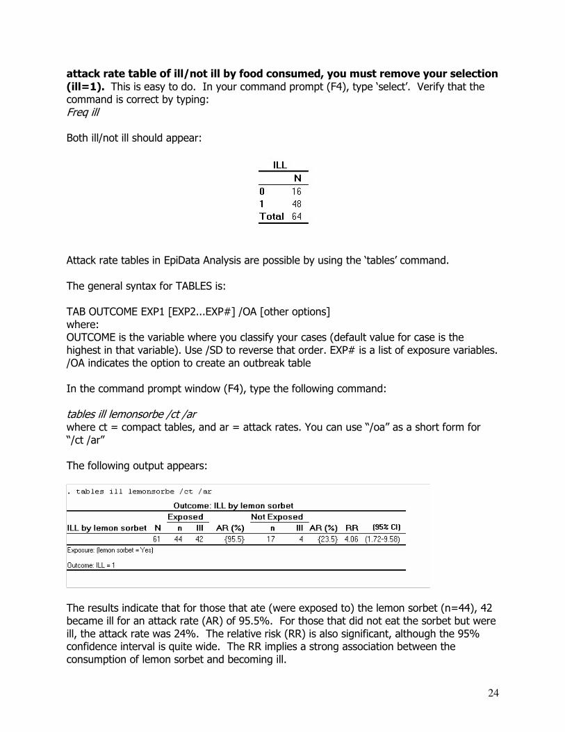
Attack rate tables in EpiData Analysis are possible by using the ‘tables’ command. The general syntax for TABLES is: TAB OUTCOME EXP1 [EXP2...EXP#] /OA [other options] where: OUTCOME is the variable where you classify your cases (default value for case is the highest in that variable). Use /SD to reverse that order. EXP# is a list of exposure variables. /OA indicates the option to create an outbreak table In the command prompt window (F4), type the following command: tables ill lemonsorbe /ct /ar where ct = compact tables, and ar = attack rates. You can use “/oa” as a short form for “/ct /ar” The following output appears:

The results indicate that for those that ate (were exposed to) the lemon sorbet (n=44), 42 became ill for an attack rate (AR) of 95.5%. For those that did not eat the sorbet but were ill, the attack rate was 24%. The relative risk (RR) is also significant, although the 95% confidence interval is quite wide. The RR implies a strong association between the consumption of lemon sorbet and becoming ill.

25

Repeat the command typing in all of the food items: tables ill lemonsorbe prosciutto caprese grilledveg cantalope fruttadima pasta farfelle freshtomat cannelloni freshherb vealmarsal chickenbre stirfryveg ovenroaste gardensala freshfruit coffee tea espresso pop juice mineralwat springwate redwine whitewine cheesecake chocolatec othercake shrimppatt pastries cookies tarts friedfishc /ct /ar Your results will look like this (only partial table shown):

You can also add a test of statistical significance to your output. Using the ill/lemon sorbet as an example, type the following: tables ill lemonsorbe /ct /ar /T where ct = compact tables, ar = attack rates and T = Chi square

The following output appears:

The warning message indicates that an expected value of less than 5 occurred in one or more cells. Therefore, the Fisher exact P value needs to be used rather than Chi square. Change the command to the following: tables ill lemonsorbe /ct /ar /ex where ct = compact tables, ar = attack rates and ex = Exact test

26

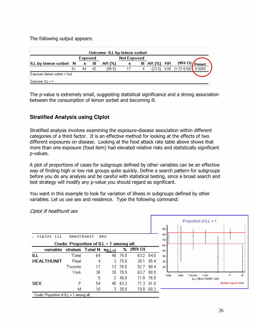
The following output appears:

The p-value is extremely small, suggesting statistical significance and a strong association between the consumption of lemon sorbet and becoming ill.

Stratified Analysis using CIplot

Stratified analysis involves examining the exposure-disease association within different categories of a third factor. It is an effective method for looking at the effects of two different exposures on disease. Looking at the food attack rate table above shows that more than one exposure (food item) had elevated relative risks and statistically significant p-values. A plot of proportions of cases for subgroups defined by other variables can be an effective way of finding high or low risk groups quite quickly. Define a search pattern for subgroups before you do any analysis and be careful with statistical testing, since a broad search and test strategy will modify any p-value you should regard as significant. You want in this example to look for variation of illness in subgroups defined by other variables. Let us use sex and residence. Type the following command:

Ciplot ill healthunit sex

27

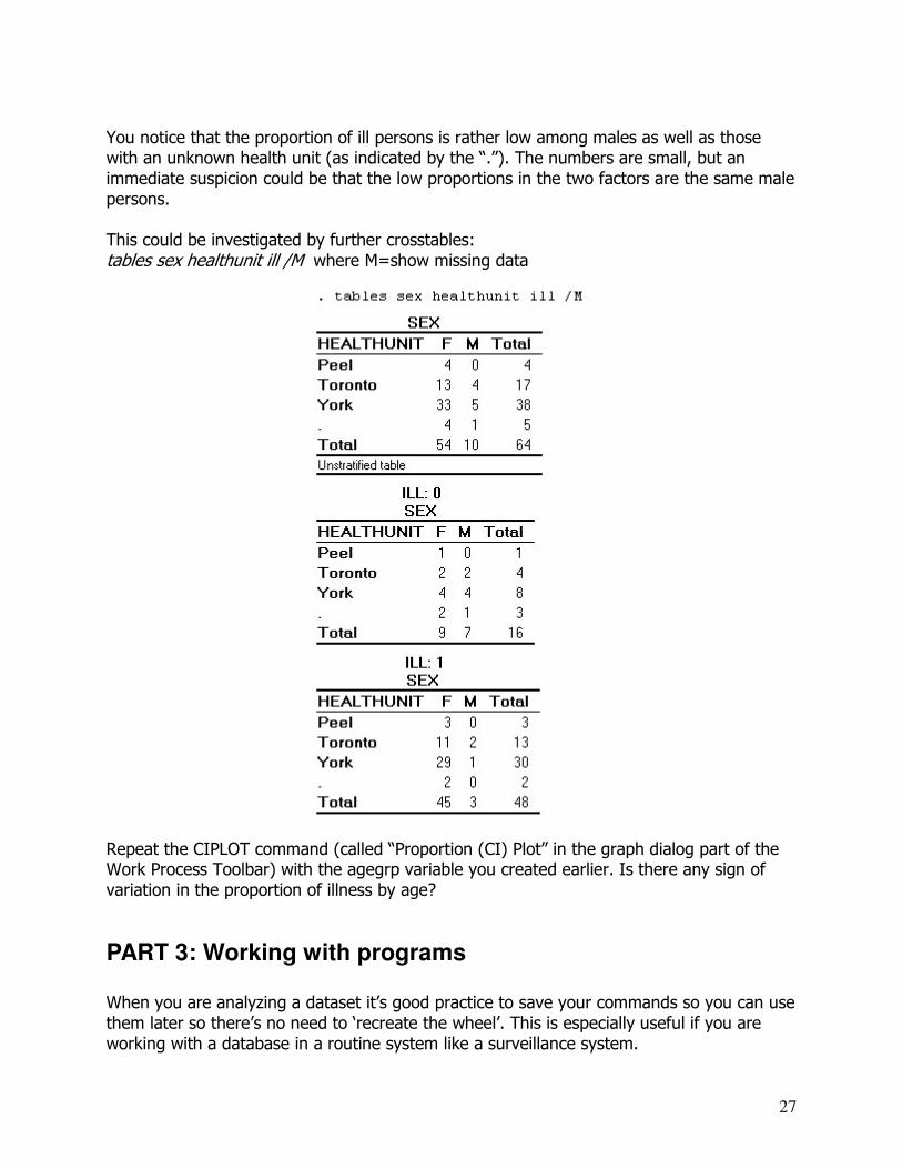
You notice that the proportion of ill persons is rather low among males as well as those with an unknown health unit (as indicated by the “.”). The numbers are small, but an immediate suspicion could be that the low proportions in the two factors are the same male persons. This could be investigated by further crosstables: tables sex healthunit ill /M where M=show missing data

Repeat the CIPLOT command (called “Proportion (CI) Plot” in the graph dialog part of the Work Process Toolbar) with the agegrp variable you created earlier. Is there any sign of variation in the proportion of illness by age?

PART 3: Working with programs When you are analyzing a dataset it’s good practice to save your commands so you can use them later so there’s no need to ‘recreate the wheel’. This is especially useful if you are working with a database in a routine system like a surveillance system.

28

You should use programs if you want to recode variables, make calculations using other variables or any other kind of manipulation. This method does not make permanent changes to your original dataset.

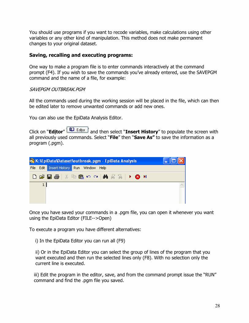
Saving, recalling and executing programs: One way to make a program file is to enter commands interactively at the command prompt (F4). If you wish to save the commands you’ve already entered, use the SAVEPGM command and the name of a file, for example: SAVEPGM OUTBREAK.PGM All the commands used during the working session will be placed in the file, which can then be edited later to remove unwanted commands or add new ones. You can also use the EpiData Analysis Editor.

Click on “Editor” and then select “Insert History” to populate the screen with all previously used commands. Select “File” then “Save As” to save the information as a program (.pgm).

Once you have saved your commands in a .pgm file, you can open it whenever you want using the EpiData Editor (FILE-->Open) To execute a program you have different alternatives: i) In the EpiData Editor you can run all (F9)

ii) Or in the EpiData Editor you can select the group of lines of the program that you want executed and then run the selected lines only (F8). With no selection only the current line is executed.

iii) Edit the program in the editor, save, and from the command prompt issue the “RUN” command and find the .pgm file you saved.

29

PART 4: Extensions to the exercises

• Creating Age category definitions. There are two approaches: A. You are going to use the “DEFINE” and "IF [logical condition] THEN [action]" commands.

In the command prompt (F4) area, write:

define agegrp # (create your age group variable as an integer) if age>=0 and age<10 then agegrp=1 if age>9 and age<20 then agegrp=2 if age>19 and age<45 then agegrp=3 if age>44 and age<65 then agegrp=4 if age>65 and age<79 then agegrp=5 * if some people have missing age, they will not get a value with the above statements, therefore you assign the value 9: if agegrp = . then agegrp = 9

* Assign value labels: labelvalue agegrp /1="0-9" /2="10-19" /3="20-44" /4="45-64" /5="65+"

B. The one used in part 1. You are going to use the “DEFINE” and "RECODE" commands.

In the command prompt (F4) area, write:

define agegrp # (create your age group variable as an integer) recode age to agegrp 0-9=1 10-19=2 20-44=3 45-64=4 65-hi=5

The command “recode” also adds the value label in the intervals indicated

• It is always good practice to view data in a graph which, for age, can conveniently be done with a box-plot and/or a cumulative plot:

Click on “Graph” And draw a box plot of age, a cumulative plot and a probit plot.

AGE

EpiData Analysis Graph

AGE

70

60

50

40

30

20

10

0

30

Questions/For More Information

Jens Lauritsen, EpiData Association www.epidata.dk Association of Public Health Epidemiologists in Ontario EpiData Expert Panel http://www.apheo.ca/index.php?pid=47

31

Appendix 1 - Importing Date/Time Fields from Excel

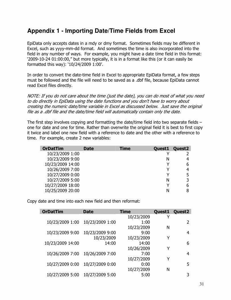
EpiData only accepts dates in a mdy or dmy format. Sometimes fields may be different in Excel, such as yyyy-mm-dd format. And sometimes the time is also incorporated into the field in any number of ways. For example, you might have a date time field in this format: ‘2009-10-24 01:00:00,” but more typically, it is in a format like this (or it can easily be formatted this way): ‘10/24/2009 1:00’. In order to convert the date-time field in Excel to appropriate EpiData format, a few steps must be followed and the file will need to be saved as a .dbf file, because EpiData cannot read Excel files directly. NOTE: If you do not care about the time (just the date), you can do most of what you need to do directly in EpiData using the date functions and you don't have to worry about creating the numeric date/time variable in Excel as discussed below. Just save the original file as a .dbf file and the date/time field will automatically contain only the date. The first step involves copying and formatting the date/time field into two separate fields – one for date and one for time. Rather than overwrite the original field it is best to first copy it twice and label one new field with a reference to date and the other with a reference to time. For example, create 2 new variables:

OrDatTim Date Time Quest1 Quest2 10/23/2009 1:00 Y 2 10/23/2009 9:00 N 4 10/23/2009 14:00 Y 6 10/26/2009 7:00 Y 4 10/27/2009 0:00 Y 5 10/27/2009 5:00 N 3 10/27/2009 18:00 Y 6 10/25/2009 20:00 N 8

Copy date and time into each new field and then reformat:

OrDatTim Date Time Quest1 Quest2

10/23/2009 1:00 10/23/2009 1:00 10/23/2009

1:00 Y

2

10/23/2009 9:00 10/23/2009 9:00 10/23/2009

9:00 N

4

10/23/2009 14:00 10/23/2009

14:00 10/23/2009

14:00 Y

6

10/26/2009 7:00 10/26/2009 7:00 10/26/2009

7:00 Y

4

10/27/2009 0:00 10/27/2009 0:00 10/27/2009

0:00 Y

5

10/27/2009 5:00 10/27/2009 5:00 10/27/2009

5:00 N

3

32

10/27/2009 18:00 10/27/2009

18:00 10/27/2009

18:00 Y

6

10/25/2009 20:00 10/25/2009

20:00 10/25/2009

20:00 N

8 Reformat by highlighting the field and clicking on ‘Format’ in the menu bar and selecting ‘Cells’. For the Date field select the ‘Category’ of Date under the first Tab ‘Number.’ For example:

The result is as follows:

OrDatTim Date Time Quest1 Quest2

10/23/2009 1:00 10/23/2009 10/23/2009

1:00 Y

2

10/23/2009 9:00 10/23/2009 10/23/2009

9:00 N

4

10/23/2009 14:00 10/23/2009 10/23/2009

14:00 Y

6

10/26/2009 7:00 10/26/2009 10/26/2009

7:00 Y

4

10/27/2009 0:00 10/27/2009 10/27/2009

0:00 Y

5

10/27/2009 5:00 10/27/2009 10/27/2009

5:00 N

3

10/27/2009 18:00 10/27/2009 10/27/2009

18:00 Y

6

10/25/2009 20:00 10/25/2009 10/25/2009

20:00 N

8 For the Time field select the ‘Category’ of Number under the first Tab ‘Number’ and set the decimal places to at least 6. For example:

33

You will now see that the time includes a value for the date, based on the number of days from Jan 01, 1900 (the reference date in Excel), and a fraction of the day made up by the time on that particular day. You can convert to hours by multiplying by 24 and convert to minutes by multiplying by (24*60). This step can be done either in Excel or in EpiData.

OrDatTim Date Time Quest1 Quest2 10/23/2009 1:00 10/23/2009 40109.041667 Y 2 10/23/2009 9:00 10/23/2009 40109.375000 N 4 10/23/2009 14:00 10/23/2009 40109.583333 Y 6 10/26/2009 7:00 10/26/2009 40112.291667 Y 4 10/27/2009 0:00 10/27/2009 40113.000000 Y 5 10/27/2009 5:00 10/27/2009 40113.208333 N 3 10/27/2009 18:00 10/27/2009 40113.750000 Y 6 10/25/2009 20:00 10/25/2009 40111.833333 N 8

At this point the file can be saved as a .dbf file. Once saved as a .dbf you can open EpiData Analysis and read the file. If you press ‘Browse’ you will see:

34

Note, however, if calculating differences between two points in time you would have to do this for each date/time variable. The advantage is that when in a numeric format, simple subtraction can be used to derive the amount of time between the events. After the difference in time has been established, which will be in days, it too can be converted to hours (multiply by 24) or minutes (multiply by another 60). For example, let's say that the exposure date/time was 10/23/2009 20:30 and the onset date/time was 10/24/2009 11:15. Using the method above, the numerical elapsed date/time for the exposure date/time would be 40109.85417. The number for the onset date/time would be 40110.46875. This yields an incubation period of: 40110.46875 - 40109.85417 = 0.61458 days, which when multiplied by 24 = 14.75 hours.