Using EpiData & Epi Info for Windows1
57
Using EpiData & Epi-Info for Windows Training for Communicable Disease Control in Local Authorities Cardiff Council (Strategic Planning & Environment) March 2007
-
Upload
hanan-ahmed -
Category
Documents
-
view
58 -
download
2
description
Epidimiology
Transcript of Using EpiData & Epi Info for Windows1

Using EpiData & Epi-Info
for Windows
Training for Communicable Disease
Control in Local Authorities
Cardiff Council (Strategic Planning & Environment)
March 2007
Acknowledgements
i
Acknowledgements
© 2007 Cardiff Council (Strategic Planning & Environment).
This training guide was produced by Alastair Tomlinson to form part of the
Communicable Disease Lead Officer Training Programme, co-ordinated by the
Wales Centre for Health.
Please send enquiries relating to this training guide to:
Alastair Tomlinson, Chartered Environmental Health Practitioner
Team Leader (Health Improvement)
Public Protection Division
Room 134 City Hall
Cathays Park
Cardiff. CF10 3ND.
029 2087 1845
About the software
Epi Info™ is a public domain software
package designed for the global community
of public health practitioners and
researchers. It provides for easy form and
database construction, data entry, and analysis with epidemiologic statistics, maps,
and graphs. Epi Info can be downloaded from http://www.cdc.gov/epiinfo
EpiData Software has developed from
securing the principles of Epi Info V6 for DOS
to an independent documentation oriented
system. EpiData can be downloaded from
http://www.epidata.dk
Conventions used in this training guide
Text to be entered on screen is shown in this font.
Directions to drop-down menu items are shown in bold type, e.g. File > SaveFile > SaveFile > SaveFile > Save.
Table of Contents
ii
Table of Contents
Acknowledgements...............................................................................i
Table of Contents .................................................................................. ii
Aim and Objectives ..............................................................................1
Outbreak Scenario................................................................................2
Creating a Questionnaire using EpiData.............................................3
Entering Data using EpiData ...............................................................17
Outbreak Investigation using Epi Info Analysis.................................19
Using Analysis with routine COSURV data.........................................35
Other capabilities of EpiData and Epi Info ........................................39
Appendix I – Comparison of Epi Info & EpiData ...............................44
Appendix II – Contents of course CD-ROM.......................................48
Appendix III – Further information & resources.................................49
Appendix IV – Worksheet for 2x2 table results .................................52
Appendix V – Check code example ................................................53
Aim and Objectives
1
Aim and Objectives
Aim of the training
To provide training on the practical use of Epi Info and EpiData in communicable
disease control, with particular reference to:
♦ An outbreak situation
♦ Analysis of routine Cosurv surveillance data
Objectives
By the end of the training delegates will:
♦ Have an understanding of EpiData and Epi-Info for Windows and their
component elements
♦ Be able to use EpiData to design a data entry form for a questionnaire in an
outbreak situation
♦ Be able to use EpiData to enter outbreak investigation data into a record
suitable for analysis in Epi Info for Windows
♦ Be able to use Analysis to obtain useful statistical and epidemiological
information from an EpiData / Epi-Info for Windows database for outbreak
investigation purposes
♦ Be able to use Analysis to import routine Cosurv surveillance data into Epi-Info
for Windows, and obtain useful statistical and epidemiological information
Outbreak Scenario
2
Outbreak Scenario
On the 17th August, you receive a telephone call from a gentleman who reports that
he and several others who attended a buffet following a funeral were suffering
symptoms of food poisoning. The buffet, provided by an external caterer, was held
at a local club following the funeral, and mourners arrived at the club at around
3.00 pm on 14th August. Food left over from the buffet was placed in the main bar
areas of the club for club members to consume later that day.
Initial activity involves obtaining of a list of people who attended the funeral and
others who may have eaten the food provided for the funeral buffet. A list of food
served at the buffet has been obtained from the caterer, and cross-referenced with
initial information gathered from cases. Indications are that around 70-80 people
attended the funeral, and approximately 40-50 of these people may have
experienced symptoms consistent with food poisoning.
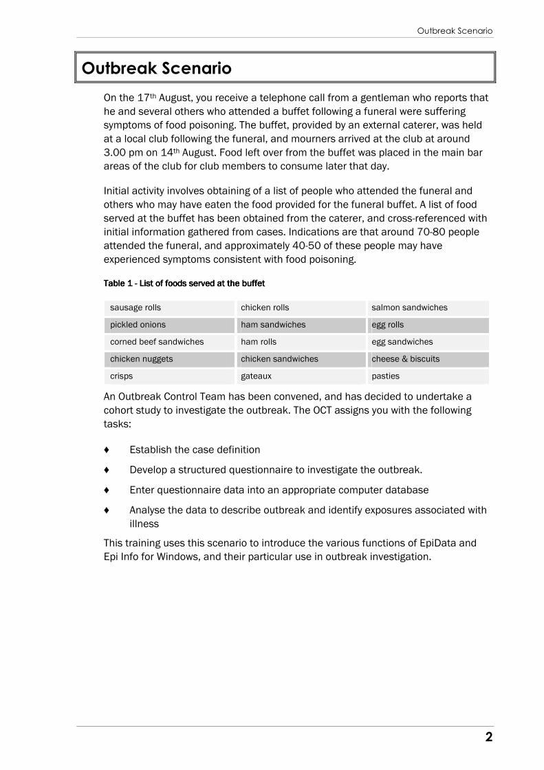
Table Table Table Table 1111 ---- List of foods served at the buffet List of foods served at the buffet List of foods served at the buffet List of foods served at the buffet
An Outbreak Control Team has been convened, and has decided to undertake a
cohort study to investigate the outbreak. The OCT assigns you with the following
tasks:
♦ Establish the case definition
♦ Develop a structured questionnaire to investigate the outbreak.
♦ Enter questionnaire data into an appropriate computer database
♦ Analyse the data to describe outbreak and identify exposures associated with
illness
This training uses this scenario to introduce the various functions of EpiData and
Epi Info for Windows, and their particular use in outbreak investigation.
sausage rolls chicken rolls salmon sandwiches
pickled onions ham sandwiches egg rolls
corned beef sandwiches ham rolls egg sandwiches
chicken nuggets chicken sandwiches cheese & biscuits
crisps gateaux pasties
Creating a Questionnaire using EpiData
3
Creating a Questionnaire using EpiData
Basic Questionnaire Creation
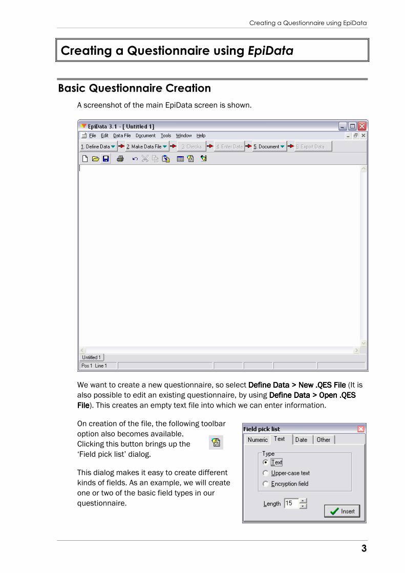
A screenshot of the main EpiData screen is shown.
We want to create a new questionnaire, so select Define DataDefine DataDefine DataDefine Data > New > New > New > New .QES File.QES File.QES File.QES File (It is
also possible to edit an existing questionnaire, by using Define Data > Open .QES Define Data > Open .QES Define Data > Open .QES Define Data > Open .QES
FileFileFileFile). This creates an empty text file into which we can enter information.
On creation of the file, the following toolbar
option also becomes available.
Clicking this button brings up the
‘Field pick list’ dialog.
This dialog makes it easy to create different
kinds of fields. As an example, we will create
one or two of the basic field types in our
questionnaire.
Creating a Questionnaire using EpiData
4
First, type an appropriate heading into the first line of your questionnaire, such as
“Lead Officer Training March 2007”.
Then, on the row below, enter Surname: Leave the cursor flashing after the colon. If
the Field pick list is not already showing, click the button to bring it on screen.
Select the ‘Text’ tab from the pick list. This then gives a short option list of ‘text’,
‘upper-case text’, and ‘encryption field’. For now we’ll accept the default ‘text’
option. Set the field length to 20, then click the Insert button. EpiData inserts a
series of underscore characters after the Surname: label. Underscore characters _
are how EpiData denotes plain text fields. The number of underscores indicates the
maximum length of the field.
On the next line, type Forename: Using the field pick list again, insert another text
field of 15 characters.
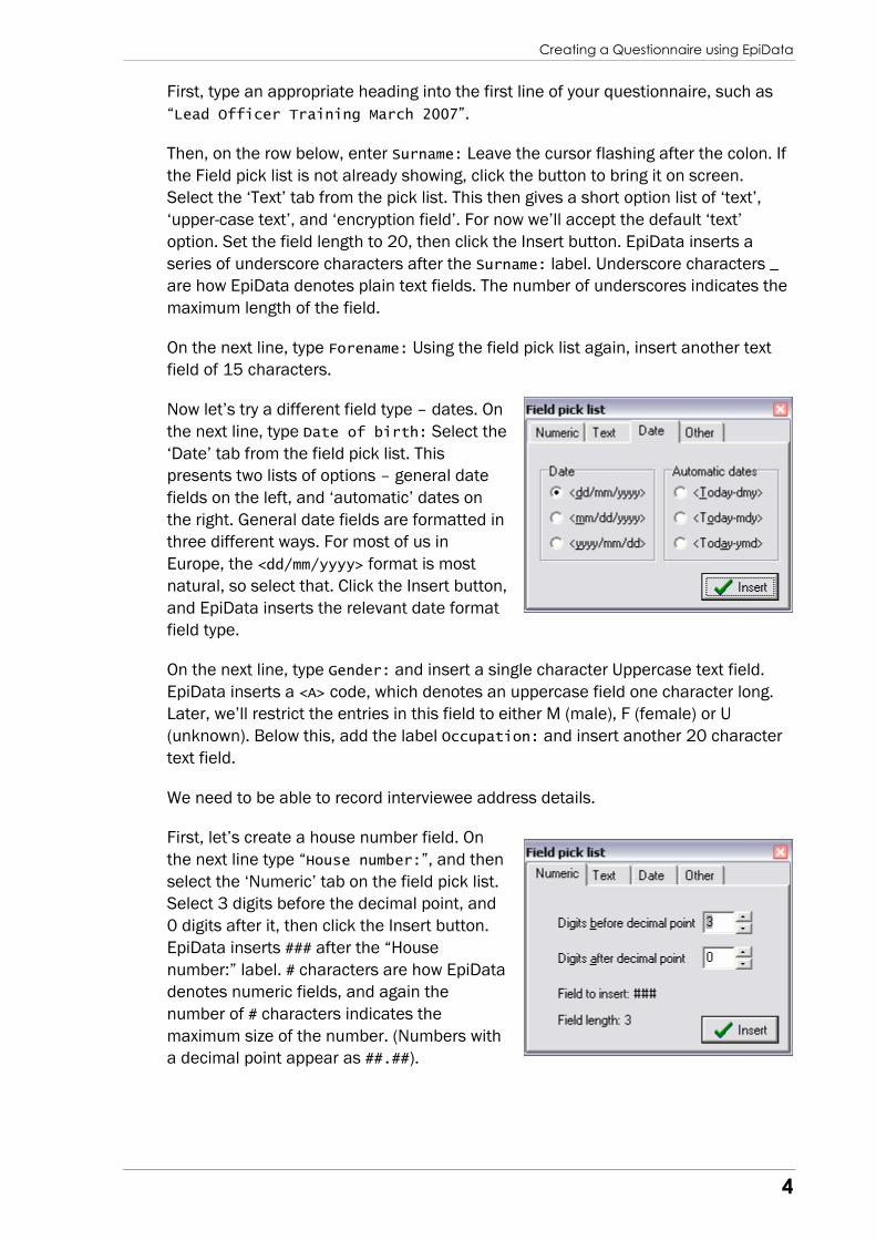
Now let’s try a different field type – dates. On
the next line, type Date of birth: Select the
‘Date’ tab from the field pick list. This
presents two lists of options – general date
fields on the left, and ‘automatic’ dates on
the right. General date fields are formatted in
three different ways. For most of us in
Europe, the <dd/mm/yyyy> format is most
natural, so select that. Click the Insert button,
and EpiData inserts the relevant date format
field type.
On the next line, type Gender: and insert a single character Uppercase text field.
EpiData inserts a <A> code, which denotes an uppercase field one character long.
Later, we’ll restrict the entries in this field to either M (male), F (female) or U
(unknown). Below this, add the label Occupation: and insert another 20 character
text field.
We need to be able to record interviewee address details.
First, let’s create a house number field. On
the next line type “House number:”, and then
select the ‘Numeric’ tab on the field pick list.
Select 3 digits before the decimal point, and
0 digits after it, then click the Insert button.
EpiData inserts ### after the “House
number:” label. # characters are how EpiData
denotes numeric fields, and again the
number of # characters indicates the
maximum size of the number. (Numbers with
a decimal point appear as ##.##).
Creating a Questionnaire using EpiData
5
Add another text field for House name (30 characters), and three more fields for
Street name (30 characters), District (20 characters) and Town (20 characters).
Then add another label for Postcode: and this time add an ‘Uppercase text’ field of
8 characters. EpiData inserts uppercase fields as <A > with the number of
spaces determining the total length of the field.
Finally, let’s add a field for telephone details. Initially it seems like a good idea to
create this as a numeric field, but in doing this we wouldn’t be able to record any
text details (such as ext. etc), and it’s unlikely we would ever want to order our data
by telephone number, so it’s probably easier to simply create a text field of around
15-20 characters. If you prefer you can create two fields, one for home and one for
other (e.g. work, mobile).
We’ve now created the fields for the basic contact details of the interviewee. Before
proceeding onto further work, let’s save what we’ve done so far. Click the Save
button on the toolbar (or select File > SaveFile > SaveFile > SaveFile > Save). Enter an appropriate filename and
location in the dialog box, and click Save.
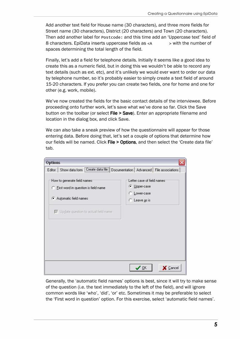
We can also take a sneak preview of how the questionnaire will appear for those
entering data. Before doing that, let’s set a couple of options that determine how
our fields will be named. Click File > OptionsFile > OptionsFile > OptionsFile > Options, and then select the ‘Create data file’
tab.
Generally, the ‘automatic field names’ options is best, since it will try to make sense
of the question (i.e. the text immediately to the left of the field), and will ignore
common words like ‘who’, ‘did’, ‘or’ etc. Sometimes it may be preferable to select
the ‘First word in question’ option. For this exercise, select ‘automatic field names’.
Creating a Questionnaire using EpiData
6
Later in the module we’ll look at how we can specifically tailor the fieldnames that
EpiData will generate in the data record files. Fieldnames have a maximum length
of 10 characters.
The decision on letter case of field names is mainly one of personal preference –
the author’s preference is to use upper-case for field names to make them stand
out.
Once you have made your option selections and clicked OK, click the Preview
Data Form button (or select Make Data File > Preview Data FormMake Data File > Preview Data FormMake Data File > Preview Data FormMake Data File > Preview Data Form).
A new tab on the main display will appear, showing the questionnaire with data
entry fields in the relevant places. You can select File > Print Data FFile > Print Data FFile > Print Data FFile > Print Data Formormormorm to get an
idea of how the questionnaire will appear on paper for completion by interviewers.
You can even practice entering data into the form to check that things appear as
you expect them to. For now, it’s useful just to see how things are going to be
presented. To close the form, select File > Close formFile > Close formFile > Close formFile > Close form, or press CTRL F4.
Currently our questionnaire lets us record interviewees’ personal details, but not a
lot else. Let’s change that by adding some details specific to the event in our
scenario. The first thing to establish is whether the person actually attended the
funeral (they may have been exposed to the food under suspicion at the club bar
after the event).
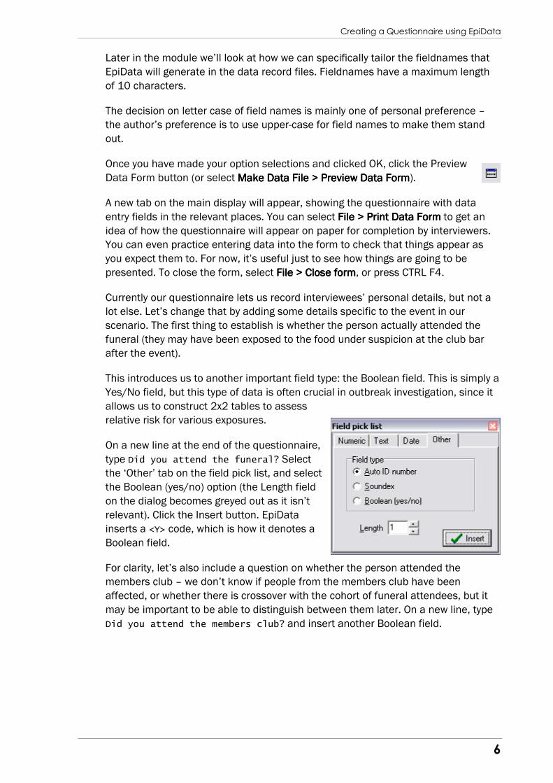
This introduces us to another important field type: the Boolean field. This is simply a
Yes/No field, but this type of data is often crucial in outbreak investigation, since it
allows us to construct 2x2 tables to assess
relative risk for various exposures.
On a new line at the end of the questionnaire,
type Did you attend the funeral? Select
the ‘Other’ tab on the field pick list, and select
the Boolean (yes/no) option (the Length field
on the dialog becomes greyed out as it isn’t
relevant). Click the Insert button. EpiData
inserts a <Y> code, which is how it denotes a
Boolean field.
For clarity, let’s also include a question on whether the person attended the
members club – we don’t know if people from the members club have been
affected, or whether there is crossover with the cohort of funeral attendees, but it
may be important to be able to distinguish between them later. On a new line, type
Did you attend the members club? and insert another Boolean field.
Creating a Questionnaire using EpiData
7
We’ll also use Boolean fields to record whether or not the person was ill, and what
their symptoms were. Add the relevant lines and fields to the questionnaire for the
following fields:
Sometimes people may have described themselves as ill, but do not meet the
actual case definition, so include an additional Case definition met? Boolean
field as well.
Another key set of data to record for those who have suffered symptoms is their
onset date/time, and the duration of symptoms. Go back up the questionnaire, and
add a couple of extra lines after Were you ill? but before the list of symptoms.
Type Onset date: and then insert a general date field. On the next line type Onset
time: and then insert a numeric field with 2 digits before and 2 digits after the
decimal point (##.##). EpiData records time-related information in this numeric,
with the digits before the point representing hours and those after minutes. The 24-
hour clock is used. Then add another field for duration of symptoms – 2 digits in
size, intended to be measured in days, and a similar 3 digit field for incubation
period, this time intended to be measured in hours.
In a full outbreak we would probably also include further questions about whether
the person was hospitalised, whether specimens had been submitted, and so on,
together with details of any other household contacts, and maybe other data to
indicate severity of symptoms, but for the purposes of this exercise we’ll skip these
elements.
The final major part of the questionnaire is the recording of relevant exposures.
Comparison of the rates of illness in those exposed and not exposed will enable us
to assess which exposures are most likely to be implicated in the outbreak. For the
purpose of this exercise, we’ll assume that the OCT has decided to focus attention
on the foods consumed at the buffet. In a real life situation, it may be more
appropriate to retain an open mind and include other potentially relevant exposures
that may explain some or all of the illness.
NB – avoid use of the ampersand & symbol in questionnaires, since it tends to
cause unexpected display results.
♦ Were you ill?
♦ Diarrhoea
♦ Vomiting
♦ Abdominal pain
♦ Nausea
♦ Pyrexia
♦ Headache
♦ Other aches
♦ Other symptoms (with a separate text
field for description)
Creating a Questionnaire using EpiData
8
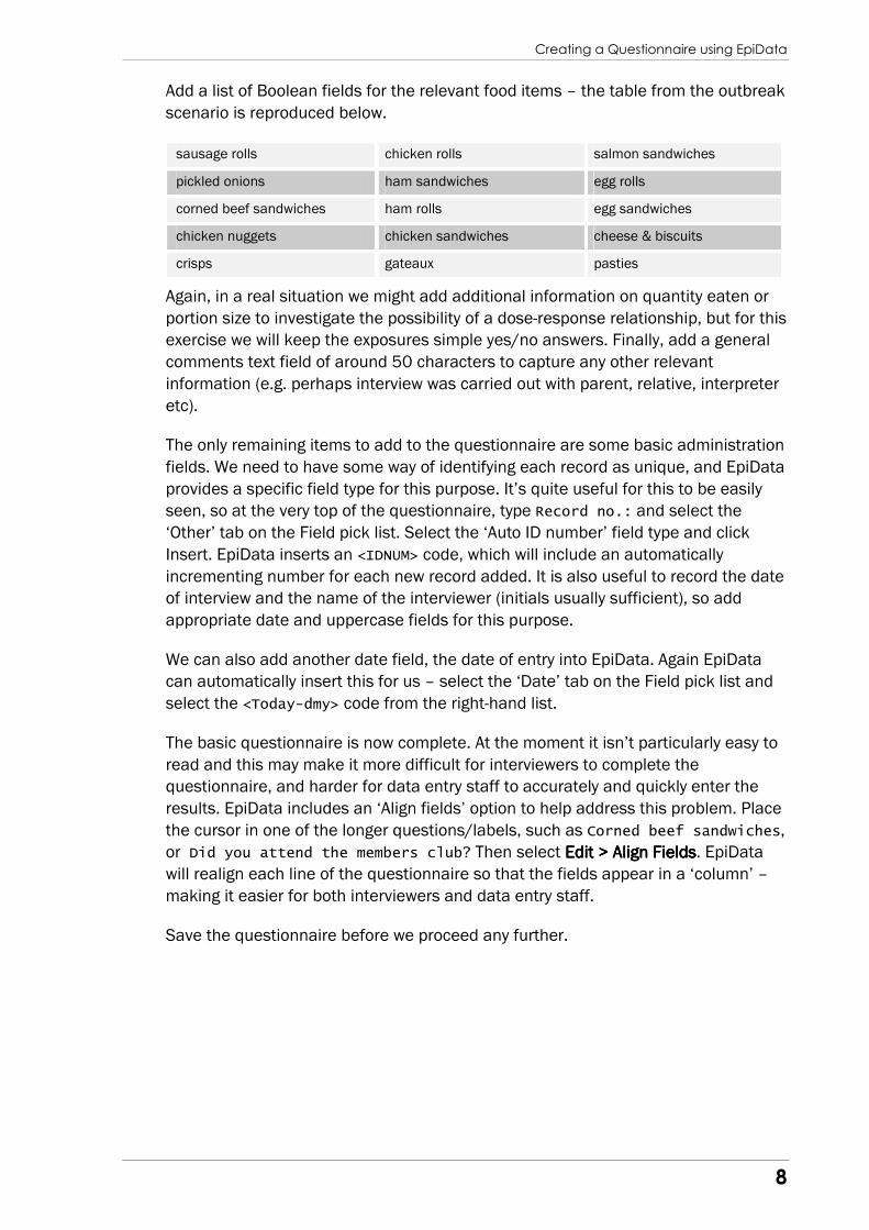
Add a list of Boolean fields for the relevant food items – the table from the outbreak
scenario is reproduced below.
Again, in a real situation we might add additional information on quantity eaten or
portion size to investigate the possibility of a dose-response relationship, but for this
exercise we will keep the exposures simple yes/no answers. Finally, add a general
comments text field of around 50 characters to capture any other relevant
information (e.g. perhaps interview was carried out with parent, relative, interpreter
etc).
The only remaining items to add to the questionnaire are some basic administration
fields. We need to have some way of identifying each record as unique, and EpiData
provides a specific field type for this purpose. It’s quite useful for this to be easily
seen, so at the very top of the questionnaire, type Record no.: and select the
‘Other’ tab on the Field pick list. Select the ‘Auto ID number’ field type and click
Insert. EpiData inserts an <IDNUM> code, which will include an automatically
incrementing number for each new record added. It is also useful to record the date
of interview and the name of the interviewer (initials usually sufficient), so add
appropriate date and uppercase fields for this purpose.
We can also add another date field, the date of entry into EpiData. Again EpiData
can automatically insert this for us – select the ‘Date’ tab on the Field pick list and
select the <Today-dmy> code from the right-hand list.
The basic questionnaire is now complete. At the moment it isn’t particularly easy to
read and this may make it more difficult for interviewers to complete the
questionnaire, and harder for data entry staff to accurately and quickly enter the
results. EpiData includes an ‘Align fields’ option to help address this problem. Place
the cursor in one of the longer questions/labels, such as Corned beef sandwiches,
or Did you attend the members club? Then select Edit > Align FieldsEdit > Align FieldsEdit > Align FieldsEdit > Align Fields. EpiData
will realign each line of the questionnaire so that the fields appear in a ‘column’ –
making it easier for both interviewers and data entry staff.
Save the questionnaire before we proceed any further.
sausage rolls chicken rolls salmon sandwiches
pickled onions ham sandwiches egg rolls
corned beef sandwiches ham rolls egg sandwiches
chicken nuggets chicken sandwiches cheese & biscuits
crisps gateaux pasties
Creating a Questionnaire using EpiData
9
Advanced questionnaire design
In this section we’ll cover some of the techniques and functions provided by
EpiData to help save time on data entry, and to ensure that accurate and reliable
data is entered.
Closer control over fieldnames
To start with, lets look at how our questionnaire looks in data entry mode. Select the
Preview Data Form button to display the data form. Use the TTTTabababab key to cycle through
the fields in the questionnaire. Note that for each field, the fieldname appears in
the status bar at the bottom left of the screen, and next to it information on the type
of data that can be entered (e.g. ‘Alpha: all entries allowed’, ‘Date (dmy): 0-
9 and / allowed’, ‘Boolean: Y,1,N,0 allowed’ etc.).
As you cycle through the fields, note the fieldnames that EpiData has automatically
assigned to each field. In the majority of cases, they make perfect sense, but there
are a few where the fieldname doesn’t intuitively indicate what the contents of the
field are. This can be particularly important where data analysis is being undertaken
by someone who wasn’t involved in the original drafting of the questionnaire (quite
conceivable in a large outbreak with several partner organisations) – the last thing
that they need is to be unsure what a relevant item of data actually means.
Fortunately, EpiData allows questionnaire designers greater control over fieldname
selection where necessary.
The default fieldname selected in each case is up to 10 letters long, based on the
text that appears immediately to the left of the field but ignoring common words
such as ‘did’ or ‘the’. As an example, the fieldname for Did you attend the
funeral? is YOUATTENDF, for Were you ill? – WEREYOUILL, and for Pickled
onions - PICKLEDONI.
For these and some other fields, we would like to tailor the fieldname to make it a
bit more meaningful. The chief way of doing this is by the use of braces { }, also
known as curly brackets. When automatically selecting fieldnames, EpiData uses
text enclosed in braces in preference to normal text. If the question is “{my} first
{field}” then the field name will be MYFIELD. Braces offer a powerful method of
defining meaningful field names.
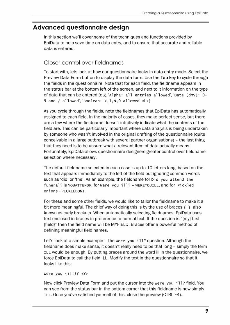
Let’s look at a simple example – the Were you ill? question. Although the
fieldname does make sense, it doesn’t really need to be that long – simply the term
ILL would be enough. By putting braces around the word ill in the questionnaire, we
force EpiData to call the field ILL. Modify the text in the questionnaire so that it
looks like this:
Were you {ill}? <Y>
Now click Preview Data Form and put the cursor into the Were you ill? field. You
can see from the status bar in the bottom corner that this fieldname is now simply
ILL. Once you’ve satisfied yourself of this, close the preview (CTRL F4).

Creating a Questionnaire using EpiData
10
This is a fairly simple example, but the EpiData capabilities are more sophisticated
than that. EpiData can pull text from more than one set of braces together to create
a fieldname. As another example, consider the Did you attend the funeral/members
club questions. Presently these have fieldnames of YOUATTENDF and YOUATTENDM
respectively – not terribly meaningful. But by changing the text in the questionnaire
as follows:
Did you {attend} the {fun}eral? <Y> Did you {attend} the members {club}? <Y>
… we produce fieldnames of ATTENDFUN and ATTENDCLUB, which are far more
intuitive. Check for yourself by clicking Preview Data Form. Notice also that the
braces do not appear on the entry form (and won’t appear on a printout either), so it
doesn’t affect the ease of use for interviewers and data entry staff.
Go through the table below to update the questions as indicated to generate more
meaningful fieldnames:
Question Current fieldname Modification New fieldname
Date of birth DATEBIRTH {D}ate {o}f {b]irth DOB
Abdominal pain ABDOMINALP {Abdom}inal {pain} ABDOMPAIN
Case definition met? CASEDEFINI {Case def}inition {met}? CASEDEFMET
Sausage rolls SAUSAGEROL {Saus}age {rolls} SAUSROLLS
Pickled onions PICKLEDONI Pickled {onions} ONIONS
Chicken nuggets CHICKENNUG Chicken {nuggets} NUGGETS
Chicken rolls CHICKENROL {Chick}en {rolls} CHICKROLLS
Chicken sandwiches CHICKENSAN {Chick}en {sand}wiches CHICKSAND
Click Preview Data Form to confirm the changes that have been made. Once you’re
finished, close the preview and save your modified questionnaire.
Controlling data entry and skipping questions
For some fields it can be useful to place restrictions on the range of data that can
be entered – for example the Gender field can only have three sensible values
(male, female, unknown) and it also makes sense to limit the Onset time field to the
valid times represented in the 24 hour clock. There also some fields that can be
filled through calculation – for example, age at time of interview, incubation period,
perhaps even case definition in some circumstances – which can help with data
accuracy and consistency. Finally data entry can be significantly quicker by using
‘skips’ so that the data entry operative doesn’t have to cycle through irrelevant
fields (such as symptom fields for an interviewee who wasn’t ill).
These functions are all achieved by what EpiData calls checks. Checks are usually
added once a ‘data file’ has been created based on the layout in a questionnaire.
Creating a Questionnaire using EpiData
11
One of the things we’ll do is add a simple calculation to work out a persons age in
years at the time of the interview. Before we create the data file, add a new numeric
field of 2 digits to hold the calculated age. Place it below the date of birth question.
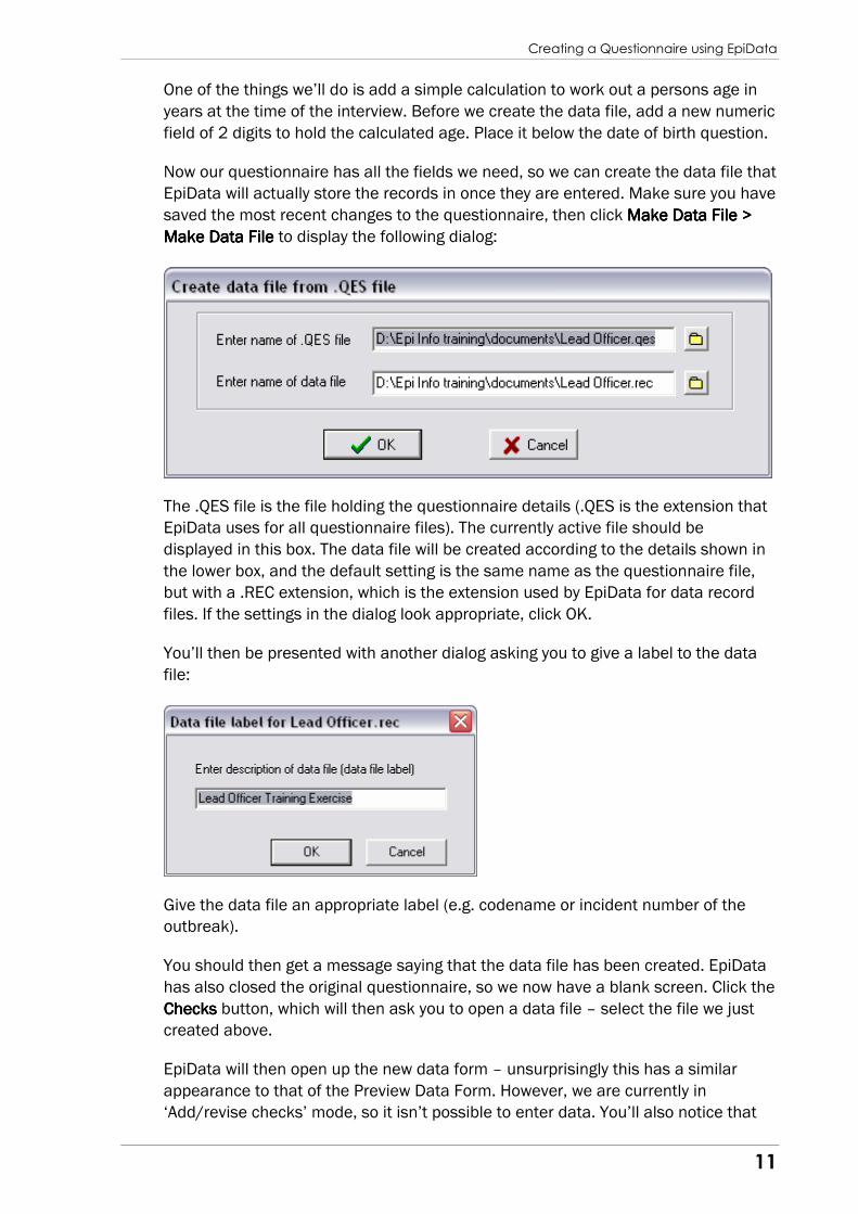
Now our questionnaire has all the fields we need, so we can create the data file that
EpiData will actually store the records in once they are entered. Make sure you have
saved the most recent changes to the questionnaire, then click MakeMakeMakeMake Data File > Data File > Data File > Data File >
Make Data FileMake Data FileMake Data FileMake Data File to display the following dialog:
The .QES file is the file holding the questionnaire details (.QES is the extension that
EpiData uses for all questionnaire files). The currently active file should be
displayed in this box. The data file will be created according to the details shown in
the lower box, and the default setting is the same name as the questionnaire file,
but with a .REC extension, which is the extension used by EpiData for data record
files. If the settings in the dialog look appropriate, click OK.
You’ll then be presented with another dialog asking you to give a label to the data
file:
Give the data file an appropriate label (e.g. codename or incident number of the
outbreak).
You should then get a message saying that the data file has been created. EpiData
has also closed the original questionnaire, so we now have a blank screen. Click the
ChecksChecksChecksChecks button, which will then ask you to open a data file – select the file we just
created above.
EpiData will then open up the new data form – unsurprisingly this has a similar
appearance to that of the Preview Data Form. However, we are currently in
‘Add/revise checks’ mode, so it isn’t possible to enter data. You’ll also notice that
Creating a Questionnaire using EpiData
12
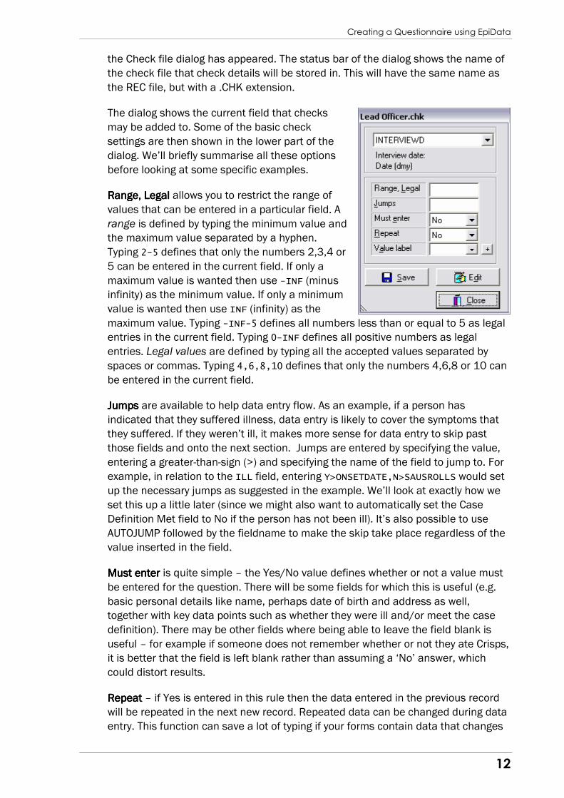
the Check file dialog has appeared. The status bar of the dialog shows the name of
the check file that check details will be stored in. This will have the same name as
the REC file, but with a .CHK extension.
The dialog shows the current field that checks
may be added to. Some of the basic check
settings are then shown in the lower part of the
dialog. We’ll briefly summarise all these options
before looking at some specific examples.
Range,Range,Range,Range, Legal Legal Legal Legal allows you to restrict the range of
values that can be entered in a particular field. A
range is defined by typing the minimum value and
the maximum value separated by a hyphen.
Typing 2-5 defines that only the numbers 2,3,4 or
5 can be entered in the current field. If only a
maximum value is wanted then use -INF (minus
infinity) as the minimum value. If only a minimum
value is wanted then use INF (infinity) as the
maximum value. Typing -INF-5 defines all numbers less than or equal to 5 as legal
entries in the current field. Typing 0-INF defines all positive numbers as legal
entries. Legal values are defined by typing all the accepted values separated by
spaces or commas. Typing 4,6,8,10 defines that only the numbers 4,6,8 or 10 can
be entered in the current field.
JumpsJumpsJumpsJumps are available to help data entry flow. As an example, if a person has
indicated that they suffered illness, data entry is likely to cover the symptoms that
they suffered. If they weren’t ill, it makes more sense for data entry to skip past
those fields and onto the next section. Jumps are entered by specifying the value,
entering a greater-than-sign (>) and specifying the name of the field to jump to. For
example, in relation to the ILL field, entering Y>ONSETDATE,N>SAUSROLLS would set
up the necessary jumps as suggested in the example. We’ll look at exactly how we
set this up a little later (since we might also want to automatically set the Case
Definition Met field to No if the person has not been ill). It’s also possible to use
AUTOJUMP followed by the fieldname to make the skip take place regardless of the
value inserted in the field.
Must enterMust enterMust enterMust enter is quite simple – the Yes/No value defines whether or not a value must
be entered for the question. There will be some fields for which this is useful (e.g.
basic personal details like name, perhaps date of birth and address as well,
together with key data points such as whether they were ill and/or meet the case
definition). There may be other fields where being able to leave the field blank is
useful – for example if someone does not remember whether or not they ate Crisps,
it is better that the field is left blank rather than assuming a ‘No’ answer, which
could distort results.
RepeatRepeatRepeatRepeat – if Yes is entered in this rule then the data entered in the previous record
will be repeated in the next new record. Repeated data can be changed during data
entry. This function can save a lot of typing if your forms contain data that changes
Creating a Questionnaire using EpiData
13
only rarely in a particular batch of forms (e.g. reporting forms in a surveillance
system). It is probably of less use in an outbreak situation.
Value labelsValue labelsValue labelsValue labels are a set of values combined with text items that explain the meaning
of each value. For example, a field is created to enter information on the sex of the
informant. It is decided that a value of 1 in the field means that the informant is
male and that a value of 2 means the informant is female. If a value label is defined
then a ‘translation table’ can be shown during data entry if the user presses [F9] (or
the [+] key on the numeric keypad). The value labels in this example would be:
1 Male 2 Female
It is important not to confuse value labels with ranges/legal values – although both
place restrictions on the data that can be entered into the field. Decide what you
want and select the appropriate option – you may not want to have to go to the
trouble of setting value labels if a simple range is all that’s required, and of course
in some situations value labels aren’t relevant.
These are the basic checks that can be attached to a field through the check file
dialog. In addition, you can click Edit to open the check file editor for the current
field and enter check code manually. This is useful for calculating field values based
on what has already been entered, and for more complicated checks (which are
largely outside the remit of this training but covered in detail in the EpiData help
files).
Let’s work through some examples.
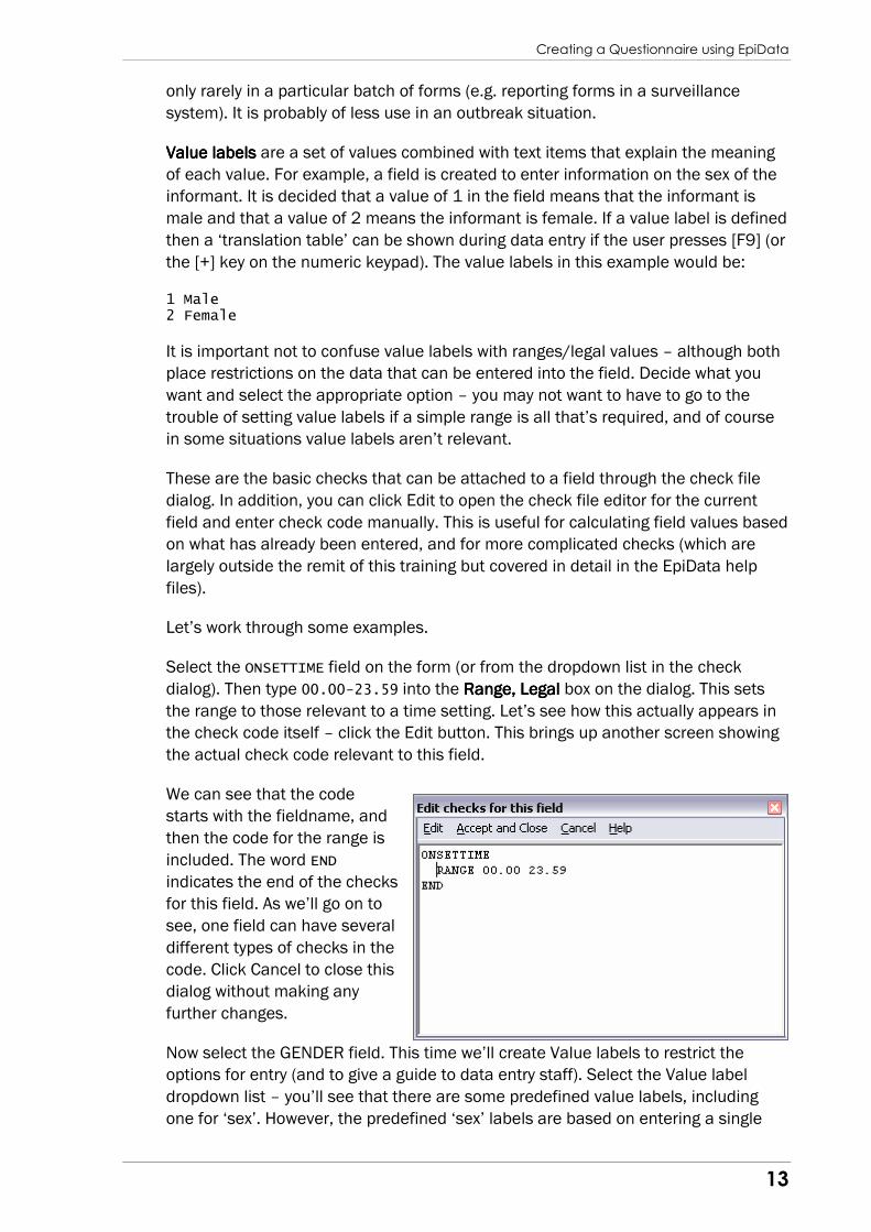
Select the ONSETTIME field on the form (or from the dropdown list in the check
dialog). Then type 00.00-23.59 into the Range, LegalRange, LegalRange, LegalRange, Legal box on the dialog. This sets
the range to those relevant to a time setting. Let’s see how this actually appears in
the check code itself – click the Edit button. This brings up another screen showing
the actual check code relevant to this field.
We can see that the code
starts with the fieldname, and
then the code for the range is
included. The word END
indicates the end of the checks
for this field. As we’ll go on to
see, one field can have several
different types of checks in the
code. Click Cancel to close this
dialog without making any
further changes.
Now select the GENDER field. This time we’ll create Value labels to restrict the
options for entry (and to give a guide to data entry staff). Select the Value label
dropdown list – you’ll see that there are some predefined value labels, including
one for ‘sex’. However, the predefined ‘sex’ labels are based on entering a single

Creating a Questionnaire using EpiData
14
digit number, and our gender field is an uppercase text field. So let’s instead create
our own value label list. Select the [none] option from the dropdown list, and then
click the + button next to the list.
The edit checks screen appears, with the following text showing:
LABEL Label_GENDER END
We then enter the legal values and relevant labels as follows:
LABEL Label_GENDER M Male F Female U Unknown END
The indenting of the text setting the labels is optional, but makes the code easier to
read. Click Accept and CloseAccept and CloseAccept and CloseAccept and Close to close the window. The value label list now shows
label_gender. This label list can be re-used for other fields if desired – perhaps not
so useful in the case of gender, but if for example you wanted to record details of
portion size in relation to each food consumed, you could define one list of value
labels (e.g. small, medium, large) and apply that to each portion size field.
There are a few fields that we would like to be entered for every questionnaire – for
example, if we do not know if the person was ill or meets the case definition, it is
difficult to draw any conclusions from any other information they have given us. So
we need to make sure that these fields are set to ‘must enter’. Select the ILL field
and change the Must enter option to Yes. Repeat this process for the CASEDEFMET,
ATTENDFUN and ATTENDCLUB fields. Initially it can be tempting to set this option for
most of the fields, but not all fields will be relevant to all interviewees (e.g.
ONSETDATE is only relevant for those who have been ill) and the blank field option
(indicating missing or unknown data) can be important in relation to exposures.
So far we’ve covered the use of ranges, value labels and must enter checks. Next,
let’s consider the use of jumps. Previously we considered that this might be useful
in controlling data entry flow after the Were you ill? question. Select the ILL field.
There are two options for the contents of the field after entry – Y or N. (By setting the
Must enter property to Yes, the ‘empty’ option is not available). Type the following
into the Jumps option:
Y>ONSETDATE
This sets the flow so that the next field selected after a Y is entered will be
ONSETDATE.
Now we need to enter the details for the N option – add a comma after the text that
is already there, then type:
N>
Creating a Questionnaire using EpiData
15
Instead of typing the name of the appropriate field to jump to, you can also select it
on the screen using the mouse – do this now by clicking on the Sausage rolls
field. EpiData automatically inserts the relevant fieldname (SAUSROLLS) into the
Jumps option.
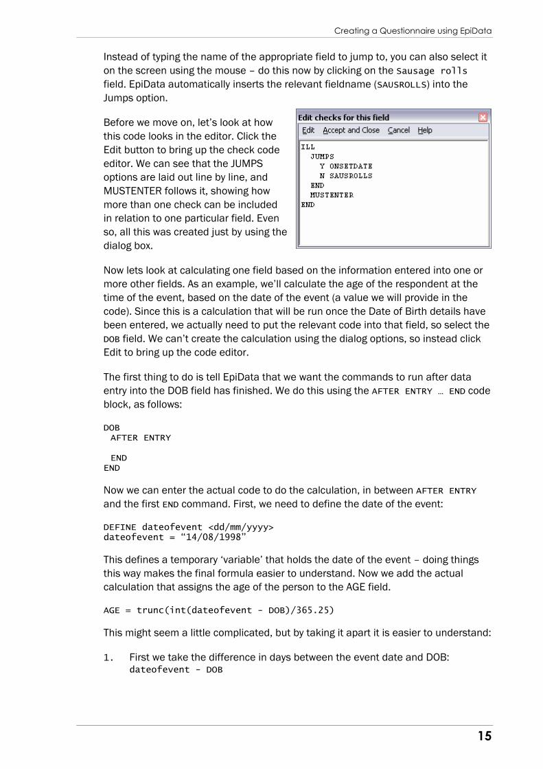
Before we move on, let’s look at how
this code looks in the editor. Click the
Edit button to bring up the check code
editor. We can see that the JUMPS
options are laid out line by line, and
MUSTENTER follows it, showing how
more than one check can be included
in relation to one particular field. Even
so, all this was created just by using the
dialog box.
Now lets look at calculating one field based on the information entered into one or
more other fields. As an example, we’ll calculate the age of the respondent at the
time of the event, based on the date of the event (a value we will provide in the
code). Since this is a calculation that will be run once the Date of Birth details have
been entered, we actually need to put the relevant code into that field, so select the
DOB field. We can’t create the calculation using the dialog options, so instead click
Edit to bring up the code editor.
The first thing to do is tell EpiData that we want the commands to run after data
entry into the DOB field has finished. We do this using the AFTER ENTRY … END code
block, as follows:
DOB AFTER ENTRY END END
Now we can enter the actual code to do the calculation, in between AFTER ENTRY
and the first END command. First, we need to define the date of the event:
DEFINE dateofevent <dd/mm/yyyy> dateofevent = “14/08/1998”
This defines a temporary ‘variable’ that holds the date of the event – doing things
this way makes the final formula easier to understand. Now we add the actual
calculation that assigns the age of the person to the AGE field.
AGE = trunc(int(dateofevent - DOB)/365.25)
This might seem a little complicated, but by taking it apart it is easier to understand:
1. First we take the difference in days between the event date and DOB: dateofevent - DOB
Creating a Questionnaire using EpiData
16
2. We convert that difference (which EpiData is still treating as a ‘date’) into an
integer, using the int function: int(dateofevent - DOB)
3. Convert the result in days to number of years, by dividing by 365.25: int(dateofevent - DOB ) / 365.25
4. It’s likely that the result of this calculation isn’t going to be a round number, so
we use the trunc function to round the result down to the person’s age in
years: trunc(int(dateofevent - DOB) / 365.25)
5. Finally we assign the result of the calculation to the AGE data field: AGE = trunc(int(dateofevent - DOB) / 365.25)
One other thing to do – since we are calculating the AGE field, we don’t need the
data entry form to actually include that field, so we can skip it and go straight to the
Gender field. We can use the Jumps section of the check dialog to do this, so
Accept and Close the code edits that you have made for the calculation and return
to the check dialog. Because we want to jump straight to the Gender field
regardless of the value entered in the DOB field, we use the AUTOJUMP term, as
follows:
AUTOJUMP GENDER
That’s all the changes we need to make, so click Save and then Close on the check
dialog.
Hopefully this makes some sense, and you can follow how check code can be used
to calculate data for a particular field. If it doesn’t, or seems too complicated, don’t
worry too much. Knowing how to use the finer points of calculations and check code
is not essential to using EpiData for outbreak investigation – but it does open up
some of the power of the program in controlling data entry and consistency, and
saving time.
On the other hand, if this has piqued your interest in using check code for running
calculations and controlling data entry, much more information on how to do this
can be found in the EpiData help files. EpiData follows largely the same check code
rules as Epi Info 6 (the DOS version of Epi Info) so if you have access to old check
code programs used in Epi Info 6, they may still work in EpiData (perhaps with some
minor tweaks).
For now, we’ve done enough to create a questionnaire to investigate this outbreak,
with some basic checks and calculations in place to help data entry. In the next
section, we’ll look briefly at how we actually enter data into our EpiData data file.
Entering Data using EpiData
17
Entering Data using EpiData
From the main EpiData screen, select the Enter DataEnter DataEnter DataEnter Data button (close any open forms
first if necessary). You’ll be asked to select a data file – choose the data (.REC) file
that you created earlier.
The data entry form that you are probably familiar with by now should appear. This
time you can enter data for real! Note also that the status bar at the bottom of the
screen has some additional buttons for navigating around records in the file.
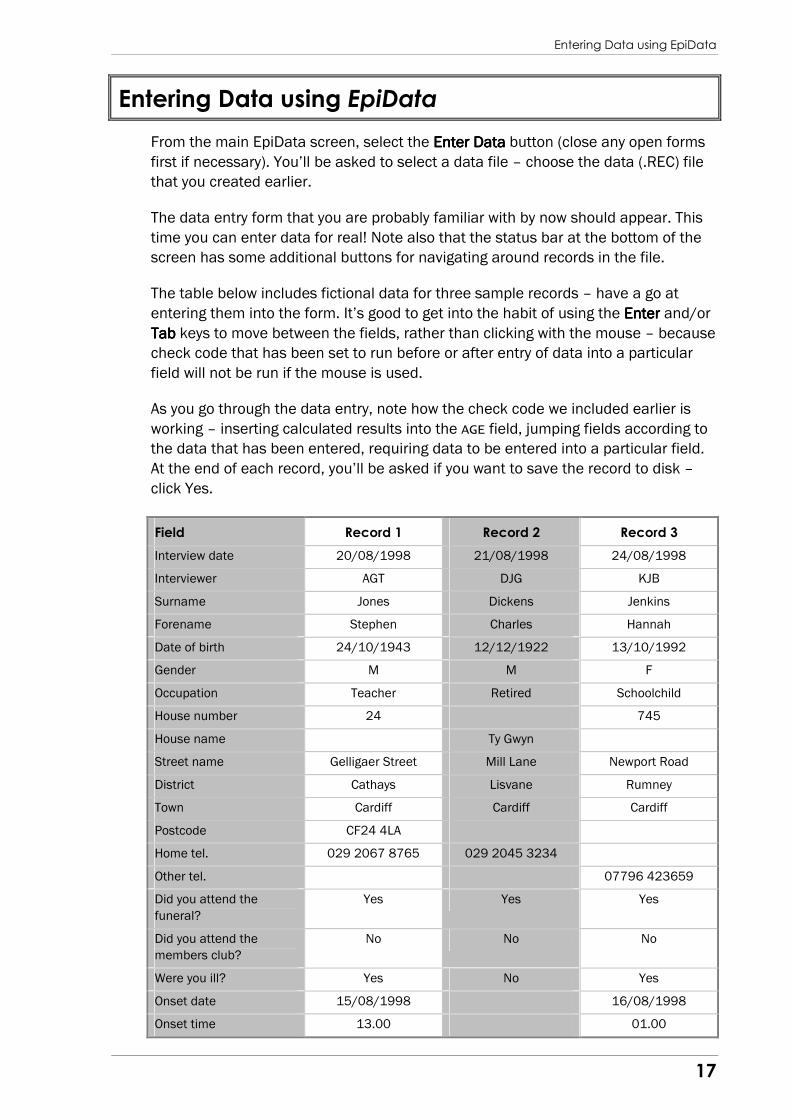
The table below includes fictional data for three sample records – have a go at
entering them into the form. It’s good to get into the habit of using the EnterEnterEnterEnter and/or
TabTabTabTab keys to move between the fields, rather than clicking with the mouse – because
check code that has been set to run before or after entry of data into a particular
field will not be run if the mouse is used.
As you go through the data entry, note how the check code we included earlier is
working – inserting calculated results into the AGE field, jumping fields according to
the data that has been entered, requiring data to be entered into a particular field.
At the end of each record, you’ll be asked if you want to save the record to disk –
click Yes.
Field Record 1 Record 2 Record 3
Interview date 20/08/1998 21/08/1998 24/08/1998
Interviewer AGT DJG KJB
Surname Jones Dickens Jenkins
Forename Stephen Charles Hannah
Date of birth 24/10/1943 12/12/1922 13/10/1992
Gender M M F
Occupation Teacher Retired Schoolchild
House number 24 745
House name Ty Gwyn
Street name Gelligaer Street Mill Lane Newport Road
District Cathays Lisvane Rumney
Town Cardiff Cardiff Cardiff
Postcode CF24 4LA
Home tel. 029 2067 8765 029 2045 3234
Other tel. 07796 423659
Did you attend the
funeral?
Yes Yes Yes
Did you attend the
members club?
No No No
Were you ill? Yes No Yes
Onset date 15/08/1998 16/08/1998
Onset time 13.00 01.00
Entering Data using EpiData
18
Duration (days) 3 4
Inc. period (hrs) 22 34
Diarrhoea Y Y
Vomiting Y N
Abdominal pain Y Y
Nausea Y N
Pyrexia N Y
Headache N Y
Other aches N N
Other symptoms Y N
Other symptoms
description Fainted
Case definition met? Y N Y
Sausage rolls Y N Y
Salmon sandwiches N Y N
Pickled onions N Y Y
Corned beef sandwiches N N N
Chicken nuggets Y N Y
Chicken rolls N Y Y
Chicken sandwiches N Y N
Ham sandwiches Y Y N
Ham rolls N N N
Egg rolls Y N Y
Egg sandwiches Y N Y
Pasties Y Y N
Crisps N N Y
Gateaux N Y Y
Cheese & biscuits Y N N
Comments Interview with mother
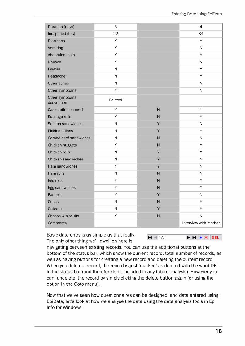
Basic data entry is as simple as that really.
The only other thing we’ll dwell on here is
navigating between existing records. You can use the additional buttons at the
bottom of the status bar, which show the current record, total number of records, as
well as having buttons for creating a new record and deleting the current record.
When you delete a record, the record is just ‘marked’ as deleted with the word DEL
in the status bar (and therefore isn’t included in any future analysis). However you
can ‘undelete’ the record by simply clicking the delete button again (or using the
option in the Goto menu).
Now that we’ve seen how questionnaires can be designed, and data entered using
EpiData, let’s look at how we analyse the data using the data analysis tools in Epi
Info for Windows.
Outbreak Investigation using Epi Info Analysis
19
Outbreak Investigation using Epi Info Analysis
For this section of the course, we’ll move to using Epi Info for Windows, and
specifically the data analysis elements of the software.1
Epi Info for Windows is based around the idea on working on projects, which are
actually based around the Microsoft Access file format. Epi Info for Windows
provides a full package for designing questionnaires, entering data and carrying out
analysis, but because EpiData’s questionnaire design tools are quicker and easier
to use, we made use of that software instead. So we need to import our EpiData
data file (which is stored in REC format, the same format used by Epi Info 6) into a
format that is usable in Epi Info for Windows.
The first thing we need to do is create an Epi Info project that we can import the
data into. We actually do this by starting the process of designing a new
questionnaire. Using the shortcut on the desktop, or via the Start menu, open the
main Epi Info for Windows menu screen. Click the Make View button to open the
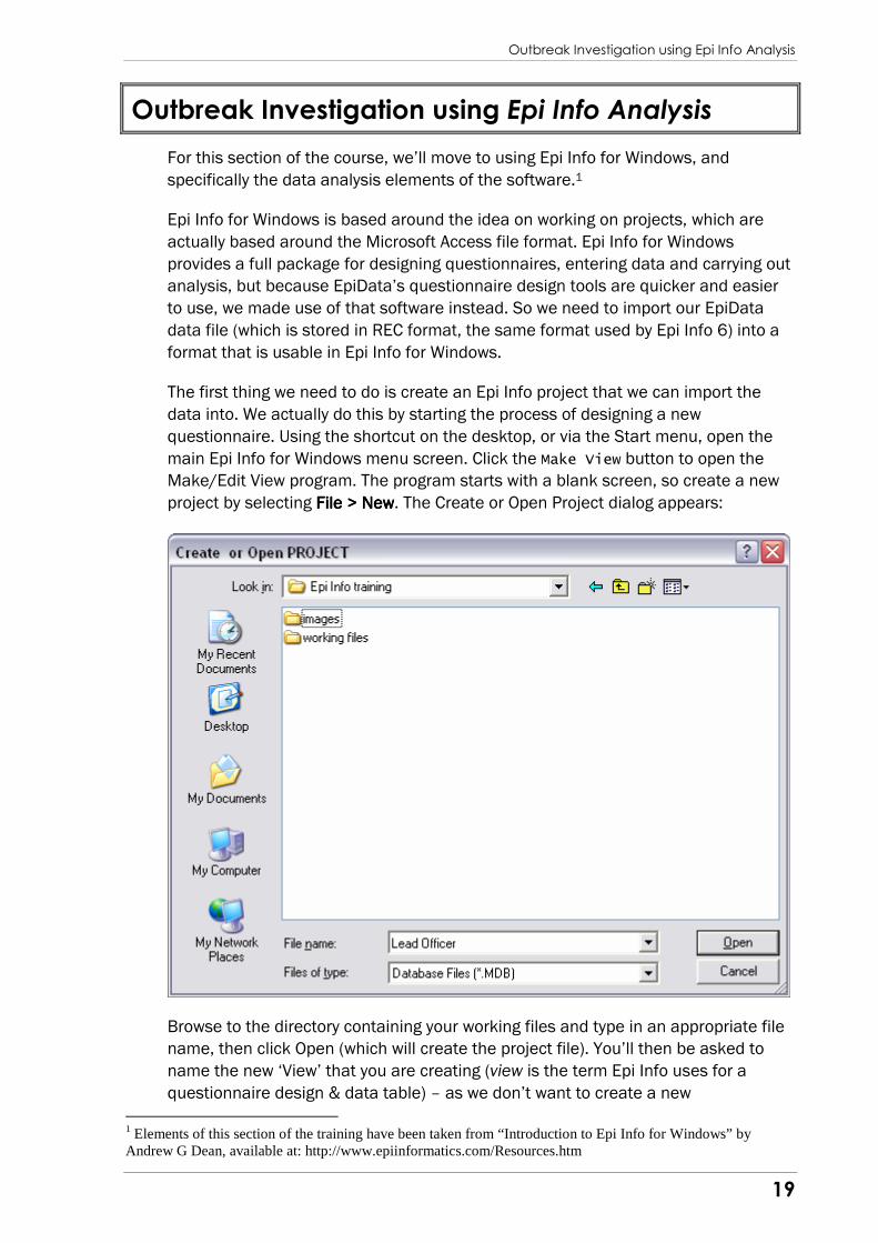
Make/Edit View program. The program starts with a blank screen, so create a new
project by selecting File > NewFile > NewFile > NewFile > New. The Create or Open Project dialog appears:
Browse to the directory containing your working files and type in an appropriate file
name, then click Open (which will create the project file). You’ll then be asked to
name the new ‘View’ that you are creating (view is the term Epi Info uses for a
questionnaire design & data table) – as we don’t want to create a new
1 Elements of this section of the training have been taken from “Introduction to Epi Info for Windows” by Andrew G Dean, available at: http://www.epiinformatics.com/Resources.htm
Outbreak Investigation using Epi Info Analysis
20
questionnaire, just click Cancel. Then select File > ExitFile > ExitFile > ExitFile > Exit to return to the main Epi Info
menu.
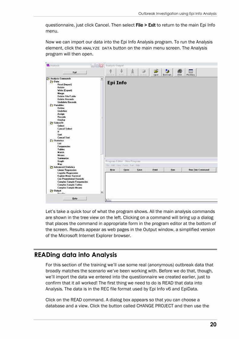
Now we can import our data into the Epi Info Analysis program. To run the Analysis
element, click the ANALYZE DATA button on the main menu screen. The Analysis
program will then open.
Let’s take a quick tour of what the program shows. All the main analysis commands
are shown in the tree view on the left. Clicking on a command will bring up a dialog
that places the command in appropriate form in the program editor at the bottom of
the screen. Results appear as web pages in the Output window, a simplified version
of the Microsoft Internet Explorer browser.
READing data into Analysis
For this section of the training we’ll use some real (anonymous) outbreak data that
broadly matches the scenario we’ve been working with. Before we do that, though,
we’ll import the data we entered into the questionnaire we created earlier, just to
confirm that it all worked! The first thing we need to do is READ that data into
Analysis. The data is in the REC file format used by Epi Info v6 and EpiData.
Click on the READ command. A dialog box appears so that you can choose a
database and a view. Click the button called CHANGE PROJECT and then use the
Outbreak Investigation using Epi Info Analysis
21
dialog that pops up to find the project file you created a moment ago. Once you’ve
found the file, select it and click the Open button to return to the main READ dialog.
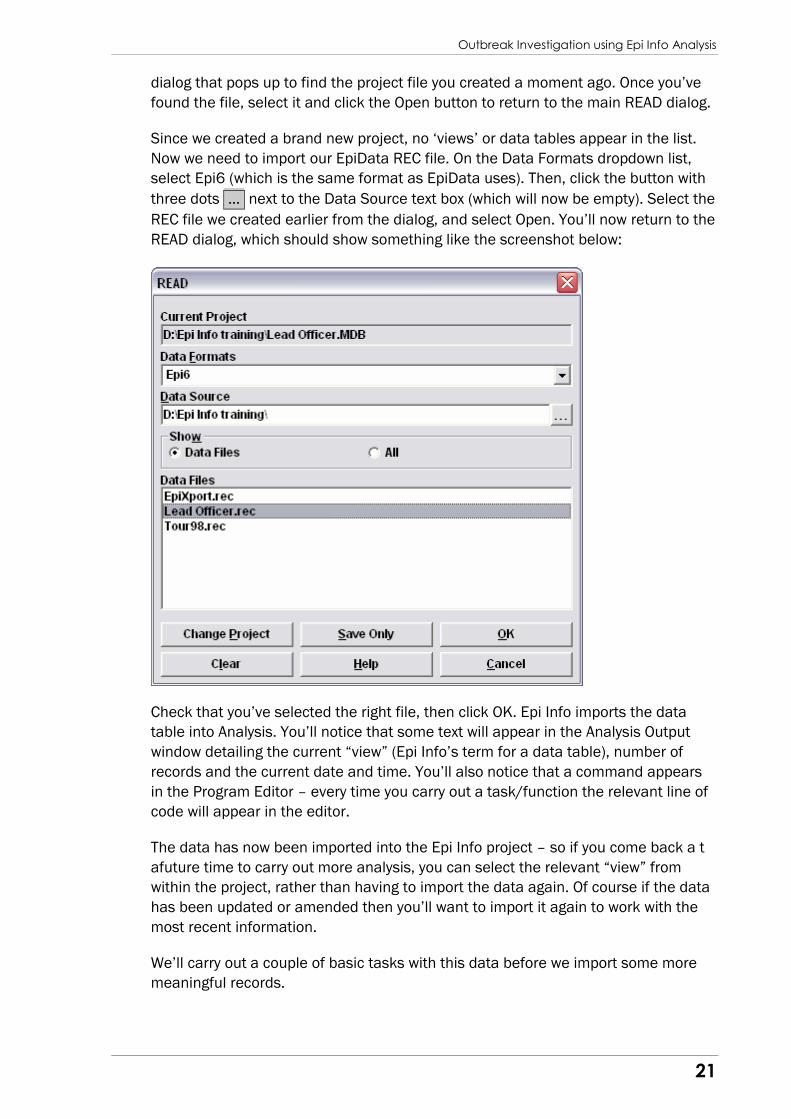
Since we created a brand new project, no ‘views’ or data tables appear in the list.
Now we need to import our EpiData REC file. On the Data Formats dropdown list,
select Epi6 (which is the same format as EpiData uses). Then, click the button with
three dots … next to the Data Source text box (which will now be empty). Select the
REC file we created earlier from the dialog, and select Open. You’ll now return to the
READ dialog, which should show something like the screenshot below:
Check that you’ve selected the right file, then click OK. Epi Info imports the data
table into Analysis. You’ll notice that some text will appear in the Analysis Output
window detailing the current “view” (Epi Info’s term for a data table), number of
records and the current date and time. You’ll also notice that a command appears
in the Program Editor – every time you carry out a task/function the relevant line of
code will appear in the editor.
The data has now been imported into the Epi Info project – so if you come back a t
afuture time to carry out more analysis, you can select the relevant “view” from
within the project, rather than having to import the data again. Of course if the data
has been updated or amended then you’ll want to import it again to work with the
most recent information.
We’ll carry out a couple of basic tasks with this data before we import some more
meaningful records.
Outbreak Investigation using Epi Info Analysis
22
LISTing basic case details
A common task in outbreak investigation is producing a simple case listing,
including for example name, gender, date of birth, case status, onset date, and so
on.
Click on LIST in the command tree. A dialog box will then appear. Initially, let’s go
with the default settings and produce a grid showing all the data, so just click OK. A
grid then appears over the top of the output window, with scrollbars etc, allowing
you to scroll through all the data currently selected. This is a bit overwhelming so we
need to change our parameters a little to limit the information that appears.
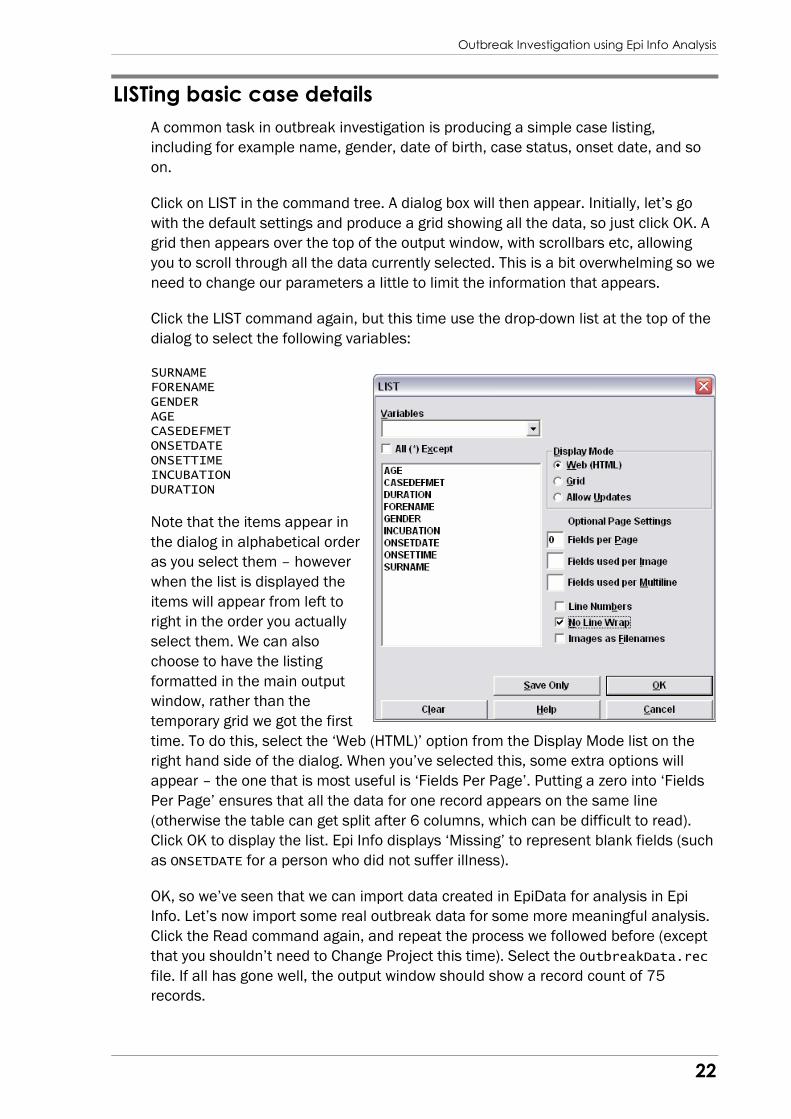
Click the LIST command again, but this time use the drop-down list at the top of the
dialog to select the following variables:
SURNAME FORENAME GENDER AGE CASEDEFMET ONSETDATE ONSETTIME INCUBATION DURATION
Note that the items appear in
the dialog in alphabetical order
as you select them – however
when the list is displayed the
items will appear from left to
right in the order you actually
select them. We can also
choose to have the listing
formatted in the main output
window, rather than the
temporary grid we got the first
time. To do this, select the ‘Web (HTML)’ option from the Display Mode list on the
right hand side of the dialog. When you’ve selected this, some extra options will
appear – the one that is most useful is ‘Fields Per Page’. Putting a zero into ‘Fields
Per Page’ ensures that all the data for one record appears on the same line
(otherwise the table can get split after 6 columns, which can be difficult to read).
Click OK to display the list. Epi Info displays ‘Missing’ to represent blank fields (such
as ONSETDATE for a person who did not suffer illness).
OK, so we’ve seen that we can import data created in EpiData for analysis in Epi
Info. Let’s now import some real outbreak data for some more meaningful analysis.
Click the Read command again, and repeat the process we followed before (except
that you shouldn’t need to Change Project this time). Select the OutbreakData.rec
file. If all has gone well, the output window should show a record count of 75
records.
Outbreak Investigation using Epi Info Analysis
23
For the rest of this section we’ll work with this data to carry out analysis that fits in
with our outbreak scenario.
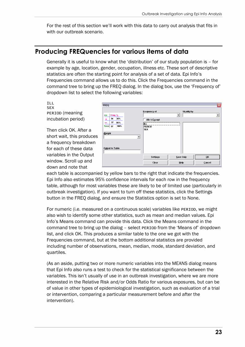
Producing FREQuencies for various items of data
Generally it is useful to know what the ‘distribution’ of our study population is – for
example by age, location, gender, occupation, illness etc. These sort of descriptive
statistics are often the starting point for analysis of a set of data. Epi Info’s
Frequencies command allows us to do this. Click the Frequencies command in the
command tree to bring up the FREQ dialog. In the dialog box, use the ‘Frequency of’
dropdown list to select the following variables:
ILL SEX
PERIOD (meaning
incubation period)
Then click OK. After a
short wait, this produces
a frequency breakdown
for each of these data
variables in the Output
window. Scroll up and
down and note that
each table is accompanied by yellow bars to the right that indicate the frequencies.
Epi Info also estimates 95% confidence intervals for each row in the frequency
table, although for most variables these are likely to be of limited use (particularly in
outbreak investigation). If you want to turn off these statistics, click the Settings
button in the FREQ dialog, and ensure the Statistics option is set to None.
For numeric (i.e. measured on a continuous scale) variables like PERIOD, we might
also wish to identify some other statistics, such as mean and median values. Epi
Info’s Means command can provide this data. Click the Means command in the
command tree to bring up the dialog – select PERIOD from the ‘Means of’ dropdown
list, and click OK. This produces a similar table to the one we got with the
Frequencies command, but at the bottom additional statistics are provided
including number of observations, mean, median, mode, standard deviation, and
quartiles.
(As an aside, putting two or more numeric variables into the MEANS dialog means
that Epi Info also runs a test to check for the statistical significance between the
variables. This isn’t usually of use in an outbreak investigation, where we are more
interested in the Relative Risk and/or Odds Ratio for various exposures, but can be
of value in other types of epidemiological investigation, such as evaluation of a trial
or intervention, comparing a particular measurement before and after the
intervention).
Outbreak Investigation using Epi Info Analysis
24
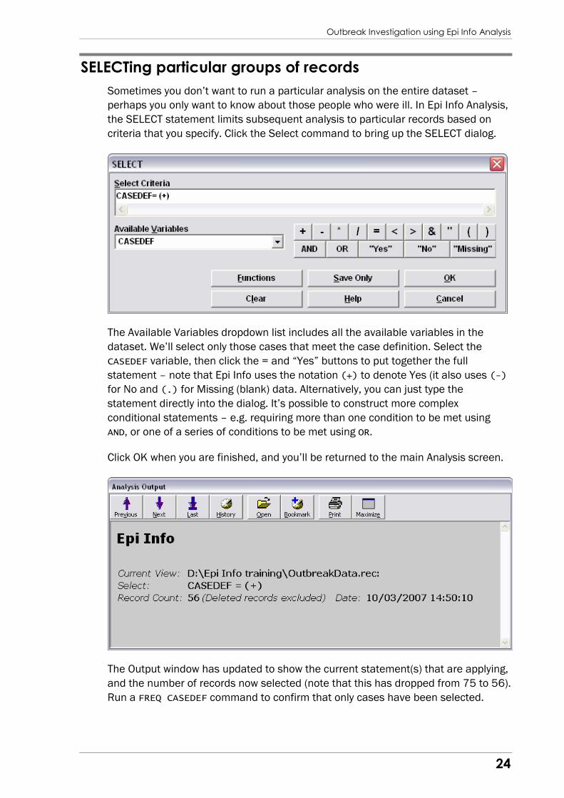
SELECTing particular groups of records
Sometimes you don’t want to run a particular analysis on the entire dataset –
perhaps you only want to know about those people who were ill. In Epi Info Analysis,
the SELECT statement limits subsequent analysis to particular records based on
criteria that you specify. Click the Select command to bring up the SELECT dialog.
The Available Variables dropdown list includes all the available variables in the
dataset. We’ll select only those cases that meet the case definition. Select the
CASEDEF variable, then click the = and “Yes” buttons to put together the full
statement – note that Epi Info uses the notation (+) to denote Yes (it also uses (-)
for No and (.) for Missing (blank) data. Alternatively, you can just type the
statement directly into the dialog. It’s possible to construct more complex
conditional statements – e.g. requiring more than one condition to be met using
AND, or one of a series of conditions to be met using OR.
Click OK when you are finished, and you’ll be returned to the main Analysis screen.
The Output window has updated to show the current statement(s) that are applying,
and the number of records now selected (note that this has dropped from 75 to 56).
Run a FREQ CASEDEF command to confirm that only cases have been selected.
Outbreak Investigation using Epi Info Analysis
25
If we now run another SELECT command, that will be processed only on the 56
records that we are currently working with (this provides another way for combining
several statements to select a particular subgroup of the data). Let’s try this by
clicking the SELECT command again. This time, we’ll select all those aged 50 or
over. Select AGE from the dropdown list of variables, then either type or use the
buttons to produce the statement AGE>=50. Click OK, and see how the Output
window has updated to reflect the second SELECT statement. Run a case LISTing of
AGE and CASEDEF to see the selected records.
To get back to the base dataset of all records, simply click the CANCEL SELECT
command, and click OK in the resulting dialog.
You’ll notice that there are also options in the same section of the command tree
for SORTing data. The dialog is self-explanatory so we won’t dwell on it here – like
the SELECT command, the SORT on the data will apply to all future analysis until a
CANCEL SORT command is issued. Before moving on, cancel any current SELECT or
SORT commands so that you are working with the base dataset again.
Recoding data
We saw earlier that, as you might expect, the individuals in our dataset are spread
across a wide range of ages. This makes it difficult to get an accurate, easily
understood picture from Frequencies or Means results about how the population is
distributed. We can overcome this problem by recoding the age data into a series of
age groups.
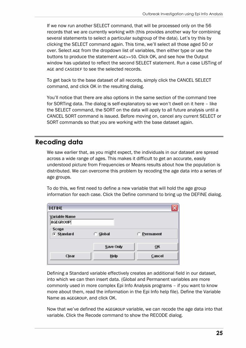
To do this, we first need to define a new variable that will hold the age group
information for each case. Click the Define command to bring up the DEFINE dialog.
Defining a Standard variable effectively creates an additional field in our dataset,
into which we can then insert data. (Global and Permanent variables are more
commonly used in more complex Epi Info Analysis programs – if you want to know
more about them, read the information in the Epi Info help file). Define the Variable
Name as AGEGROUP, and click OK.
Now that we’ve defined the AGEGROUP variable, we can recode the age data into that
variable. Click the Recode command to show the RECODE dialog.
Outbreak Investigation using Epi Info Analysis
26
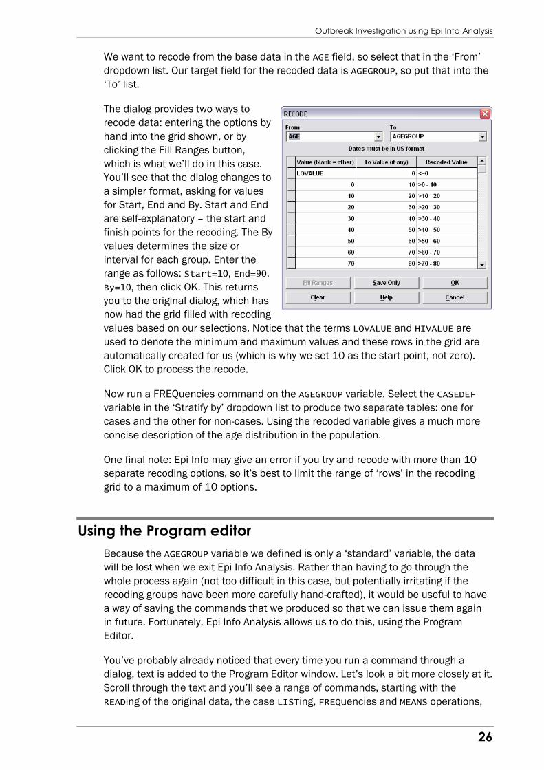
We want to recode from the base data in the AGE field, so select that in the ‘From’
dropdown list. Our target field for the recoded data is AGEGROUP, so put that into the
‘To’ list.
The dialog provides two ways to
recode data: entering the options by
hand into the grid shown, or by
clicking the Fill Ranges button,
which is what we’ll do in this case.
You’ll see that the dialog changes to
a simpler format, asking for values
for Start, End and By. Start and End
are self-explanatory – the start and
finish points for the recoding. The By
values determines the size or
interval for each group. Enter the
range as follows: Start=10, End=90,
By=10, then click OK. This returns
you to the original dialog, which has
now had the grid filled with recoding
values based on our selections. Notice that the terms LOVALUE and HIVALUE are
used to denote the minimum and maximum values and these rows in the grid are
automatically created for us (which is why we set 10 as the start point, not zero).
Click OK to process the recode.
Now run a FREQuencies command on the AGEGROUP variable. Select the CASEDEF
variable in the ‘Stratify by’ dropdown list to produce two separate tables: one for
cases and the other for non-cases. Using the recoded variable gives a much more
concise description of the age distribution in the population.
One final note: Epi Info may give an error if you try and recode with more than 10
separate recoding options, so it’s best to limit the range of ‘rows’ in the recoding
grid to a maximum of 10 options.
Using the Program editor
Because the AGEGROUP variable we defined is only a ‘standard’ variable, the data
will be lost when we exit Epi Info Analysis. Rather than having to go through the
whole process again (not too difficult in this case, but potentially irritating if the
recoding groups have been more carefully hand-crafted), it would be useful to have
a way of saving the commands that we produced so that we can issue them again
in future. Fortunately, Epi Info Analysis allows us to do this, using the Program
Editor.
You’ve probably already noticed that every time you run a command through a
dialog, text is added to the Program Editor window. Let’s look a bit more closely at it.
Scroll through the text and you’ll see a range of commands, starting with the
READing of the original data, the case LISTing, FREQuencies and MEANS operations,
Outbreak Investigation using Epi Info Analysis
27
SELECTing and SORTing of records. At the bottom of the text will be the most recent
commands, including DEFINE AGEGROUP and the RECODE commands.
The Program Editor allows us to save this output into the project as an Epi Info
Program. We could save this entire output as a program in Epi Info, and then
running it again at another date would process all the commands listed one after
another. That’s probably overkill, though, and would take a significant amount of
processing time to come up with the results. More usefully, we could save the
commands relevant to the recoding process. Go through the text in the editor and
delete everything that appears before the DEFINE AGEGROUP statement. Then delete
any text after the END statement at the end of the RECODE code block. The Program
Editor should now contain text that looks something like this:
DEFINE AGEGROUP RECODE AGE TO AGEGROUP LOVALUE - 10 = "<=10" 10 - 20 = ">10 - 20" 20 - 30 = ">20 - 30" 30 - 40 = ">30 - 40" 40 - 50 = ">40 - 50" 50 - 60 = ">50 - 60" 60 - 70 = ">60 - 70" 70 - 80 = ">70 - 80" 80 - 90 = ">80 - 90" 90 - HIVALUE = ">90" END
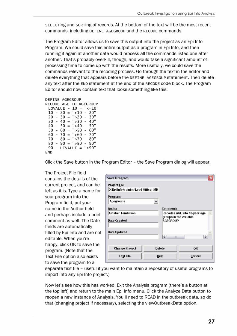
Click the Save button in the Program Editor – the Save Program dialog will appear:
The Project File field
contains the details of the
current project, and can be
left as it is. Type a name for
your program into the
Program field, put your
name in the Author field
and perhaps include a brief
comment as well. The Date
fields are automatically
filled by Epi Info and are not
editable. When you’re
happy, click OK to save the
program. (Note that the
Text File option also exists
to save the program to a
separate text file – useful if you want to maintain a repository of useful programs to
import into any Epi Info project.)
Now let’s see how this has worked. Exit the Analysis program (there’s a button at
the top left) and return to the main Epi Info menu. Click the Analyze Data button to
reopen a new instance of Analysis. You’ll need to READ in the outbreak data, so do
that (changing project if necessary), selecting the viewOutbreakData option.

Outbreak Investigation using Epi Info Analysis
28
Once the data has been read into Analysis, click the Open button on the Program
Editor. The Read Program dialog will appear – this looks very similar to the Save
Program dialog. Click the Program dropdown list and select the program you stored
earlier – the author, date and comment details will then appear. Click OK to read
the program into the Program Editor. The program hasn’t yet been run, so click the
Run button (note that the Run Command button runs only the command currently
containing the cursor). Since all the commands in our program don’t actually
produce any output of their own, we need to run FREQ AGEGROUP to see if things
have worked. You should get the same age group breakdown that we saw a little
earlier.
Accessing previous results & controlling file storage
By now, you might be wondering where all this Analysis output is being stored. Epi
Info Analysis stores output as HTML files (web pages). By default, these files are
stored in the same folder as the project file, but there are several options available
to customise this in the ‘Output’ section towards the bottom of the command tree.
Epi Info also provides a handy index of all the output that you’ve produced in work
on the project. First, click on CLOSEOUT to close the output file you’ve just been
working on, and then click on the hyperlink called RESULTS LIBRARY at the top of
the output in the browser (you might need to scroll up). An index page appears,
showing previous commands that have produced output files. Click on any of the
entries to display it.
There are a wide range of options for customising storage of data, mostly accessed
via the Storing Output command. The most useful of these is the ability to set the
‘Results Folder’ where output files are stored – perhaps a new subfolder inside your
main project directory. Other settings for archiving data are also available, but get
more involved – refer to the Epi Info help file for more details.
Despite all this, there might come a time when you want to define a specific file in
which to store a particular set of output. In the next section, we’ll be producing
some graphs, so now we’ll create a file specifically to store the graph output in. This
is does using the Routeout command, which pops up a simple dialog asking for an
output filename.
Click the … button to bring
up the file browser dialog –
enter a file name (like
Graphs) and click the Open
button, then click OK in the
main ROUTEOUT dialog.
Any future output will be directed to this file, until a CLOSEOUT command is issued
(when Epi Info will start issuing output files in the default location again.)
Outbreak Investigation using Epi Info Analysis
29
Producing simple GRAPHs
A common task in outbreak investigation is to plot an epidemic curve showing the
order and frequency of onset date. Epi Info Analysis has a Graph command that
helps us do this.
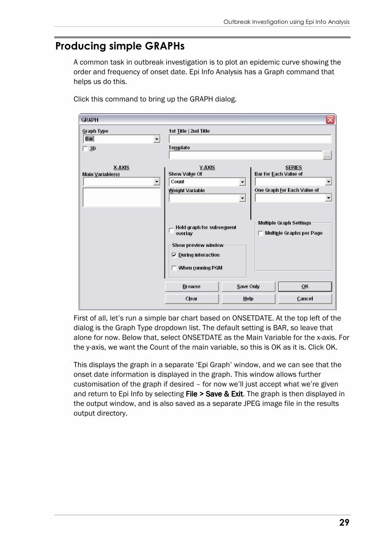
Click this command to bring up the GRAPH dialog.
First of all, let’s run a simple bar chart based on ONSETDATE. At the top left of the
dialog is the Graph Type dropdown list. The default setting is BAR, so leave that
alone for now. Below that, select ONSETDATE as the Main Variable for the x-axis. For
the y-axis, we want the Count of the main variable, so this is OK as it is. Click OK.
This displays the graph in a separate ‘Epi Graph’ window, and we can see that the
onset date information is displayed in the graph. This window allows further
customisation of the graph if desired – for now we’ll just accept what we’re given
and return to Epi Info by selecting File > Save & ExitFile > Save & ExitFile > Save & ExitFile > Save & Exit. The graph is then displayed in
the output window, and is also saved as a separate JPEG image file in the results
output directory.
Outbreak Investigation using Epi Info Analysis
30
Unfortunately, this graph isn’t terribly helpful – because the incubation period is
relatively short, separating the cases in hours would be more useful. Fortunately,
the outbreak investigators in this case included a field for incubation period in their
data collection, measured in hours. Previously we ran a MEANS command on the
PERIOD variable, so we know that there is a wide range of values from 5 to 46 hours
– and around 30 different values in each case. Producing a Bar chart in this
instance may not be terribly helpful, since we’ll get the same wide range of values –
because a bar chart will produce a bar for each individual value represented in the
data set. But because we’re using a numerical (continuous) field, we can run a
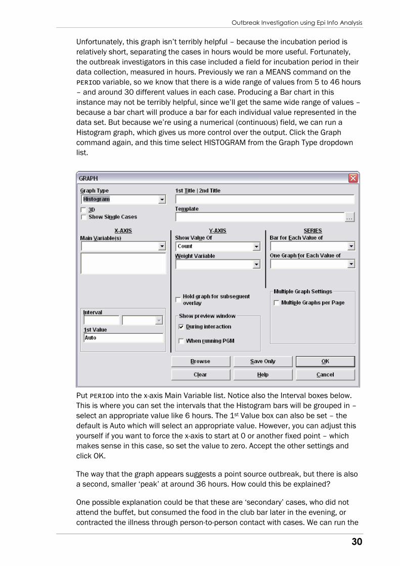
Histogram graph, which gives us more control over the output. Click the Graph
command again, and this time select HISTOGRAM from the Graph Type dropdown
list.
Put PERIOD into the x-axis Main Variable list. Notice also the Interval boxes below.
This is where you can set the intervals that the Histogram bars will be grouped in –
select an appropriate value like 6 hours. The 1st Value box can also be set – the
default is Auto which will select an appropriate value. However, you can adjust this
yourself if you want to force the x-axis to start at 0 or another fixed point – which
makes sense in this case, so set the value to zero. Accept the other settings and
click OK.
The way that the graph appears suggests a point source outbreak, but there is also
a second, smaller ‘peak’ at around 36 hours. How could this be explained?
One possible explanation could be that these are ‘secondary’ cases, who did not
attend the buffet, but consumed the food in the club bar later in the evening, or
contracted the illness through person-to-person contact with cases. We can run the
Outbreak Investigation using Epi Info Analysis
31
graph again, and this time separate the data into two ‘series’, based on whether or
not the case attended the funeral itself. Open the GRAPH dialog again, select
HISTOGRAM as the graph type, PERIOD as the main variable, and an interval of 6
hours, with a 1st value of zero. We still want a count of cases on the y-axis, but we
also want to display bars for the series – so select the variable ATTEND in the ‘Bar
for each value of …” dropdown list. It is possible to set the title, but we can do this
at the customisation stage, so we’ll look at that in a moment.
Click OK to produce the graph in Epi Graph. Now we can see that there are two
separate sets of bars for those who did and did not attend the funeral.
Nevertheless, by customising the graph we can make it easier to see exactly what’s
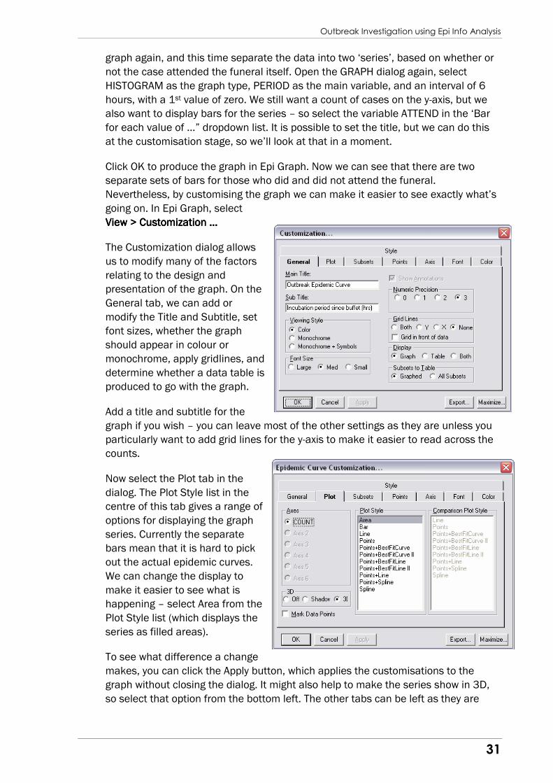
going on. In Epi Graph, select
View > Customization …View > Customization …View > Customization …View > Customization …
The Customization dialog allows
us to modify many of the factors
relating to the design and
presentation of the graph. On the
General tab, we can add or
modify the Title and Subtitle, set
font sizes, whether the graph
should appear in colour or
monochrome, apply gridlines, and
determine whether a data table is
produced to go with the graph.
Add a title and subtitle for the
graph if you wish – you can leave most of the other settings as they are unless you
particularly want to add grid lines for the y-axis to make it easier to read across the
counts.
Now select the Plot tab in the
dialog. The Plot Style list in the
centre of this tab gives a range of
options for displaying the graph
series. Currently the separate
bars mean that it is hard to pick
out the actual epidemic curves.
We can change the display to
make it easier to see what is
happening – select Area from the
Plot Style list (which displays the
series as filled areas).
To see what difference a change
makes, you can click the Apply button, which applies the customisations to the
graph without closing the dialog. It might also help to make the series show in 3D,
so select that option from the bottom left. The other tabs can be left as they are
Outbreak Investigation using Epi Info Analysis
32
unless you would like to change the Font, Color or Styles used for the display –
these tabs are self-explanatory.
Access to many of these settings can also be obtained by right-clicking on the graph
and selecting from the pop-up menu options that appear.
Once you’re happy with the settings, click OK in the dialog to have a proper look at
your graph. It’s now easier to see what’s been happening. When you’re finished you
can select File > Save & ExitFile > Save & ExitFile > Save & ExitFile > Save & Exit to return to the Analysis window. (You can also select
File > ExportFile > ExportFile > ExportFile > Export to export the graph as an image to the clipboard, direct to a printer, or
a file location of your choice).
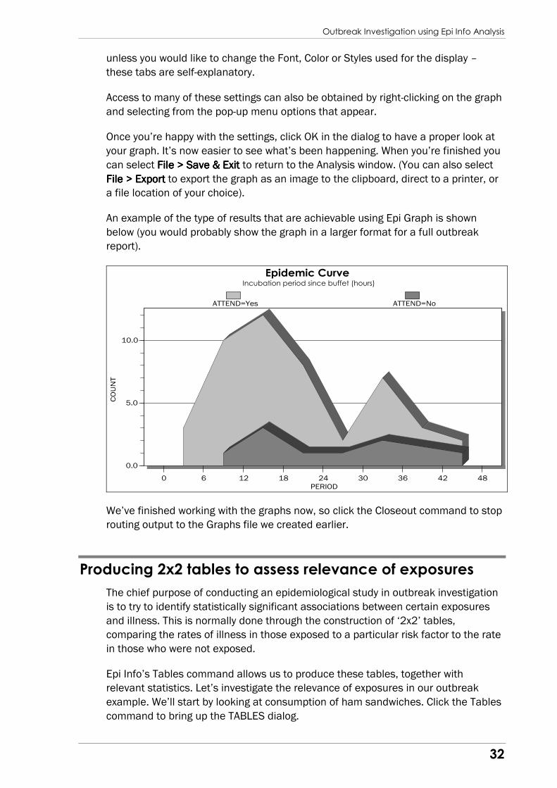
An example of the type of results that are achievable using Epi Graph is shown
below (you would probably show the graph in a larger format for a full outbreak
report).
0.0
5.0
10.0
0 6 12 18 24 30 36 42 48
Epidemic CurveIncubation period since buffet (hours)
COUNT
PERIOD
ATTEND=Yes ATTEND=No
We’ve finished working with the graphs now, so click the Closeout command to stop
routing output to the Graphs file we created earlier.
Producing 2x2 tables to assess relevance of exposures
The chief purpose of conducting an epidemiological study in outbreak investigation
is to try to identify statistically significant associations between certain exposures
and illness. This is normally done through the construction of ‘2x2’ tables,
comparing the rates of illness in those exposed to a particular risk factor to the rate
in those who were not exposed.
Epi Info’s Tables command allows us to produce these tables, together with
relevant statistics. Let’s investigate the relevance of exposures in our outbreak
example. We’ll start by looking at consumption of ham sandwiches. Click the Tables
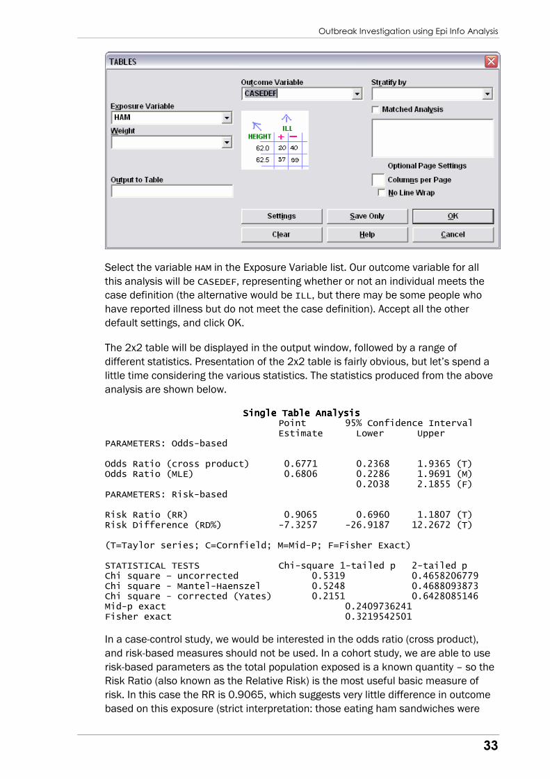
command to bring up the TABLES dialog.
Outbreak Investigation using Epi Info Analysis
33
Select the variable HAM in the Exposure Variable list. Our outcome variable for all
this analysis will be CASEDEF, representing whether or not an individual meets the
case definition (the alternative would be ILL, but there may be some people who
have reported illness but do not meet the case definition). Accept all the other
default settings, and click OK.
The 2x2 table will be displayed in the output window, followed by a range of
different statistics. Presentation of the 2x2 table is fairly obvious, but let’s spend a
little time considering the various statistics. The statistics produced from the above
analysis are shown below.
Single Table AnalysisSingle Table AnalysisSingle Table AnalysisSingle Table Analysis Point 95% Confidence Interval Estimate Lower Upper PARAMETERS: Odds-based Odds Ratio (cross product) 0.6771 0.2368 1.9365 (T) Odds Ratio (MLE) 0.6806 0.2286 1.9691 (M) 0.2038 2.1855 (F) PARAMETERS: Risk-based Risk Ratio (RR) 0.9065 0.6960 1.1807 (T) Risk Difference (RD%) -7.3257 -26.9187 12.2672 (T) (T=Taylor series; C=Cornfield; M=Mid-P; F=Fisher Exact) STATISTICAL TESTS Chi-square 1-tailed p 2-tailed p Chi square – uncorrected 0.5319 0.4658206779 Chi square - Mantel-Haenszel 0.5248 0.4688093873 Chi square - corrected (Yates) 0.2151 0.6428085146 Mid-p exact 0.2409736241 Fisher exact 0.3219542501
In a case-control study, we would be interested in the odds ratio (cross product),
and risk-based measures should not be used. In a cohort study, we are able to use
risk-based parameters as the total population exposed is a known quantity – so the
Risk Ratio (also known as the Relative Risk) is the most useful basic measure of
risk. In this case the RR is 0.9065, which suggests very little difference in outcome
based on this exposure (strict interpretation: those eating ham sandwiches were

Outbreak Investigation using Epi Info Analysis
34
0.9065 times as likely to be cases as those who did not). Since the 95% Confidence
Interval includes the ‘no difference’ value of 1, we know that this difference is not
statistically significant at the 95% confidence level.
The statistics provided also include chi-square test results in the form of p-values,
achieved by a number of different statistical procedures. In general, where a
reasonably large dataset/sample size has been used, there is unlikely to be an
important difference between these procedures. However, where the differences
between the procedures are important (e.g. one identifies a statistically significant
result, but another does not), you should seek the advice of an epidemiologist or
statistician to assist with interpretation of the results.
This analysis indicates that consumption of ham sandwiches was not associated
with illness in this outbreak. However, other foodstuffs might be implicated in the
outbreak, and assessments of the strength of association between consumption
and illness for each of the menu items should be completed.
Appendix IV Appendix IV Appendix IV Appendix IV containscontainscontainscontains a a a a worksheet containing an empty table for you to record the worksheet containing an empty table for you to record the worksheet containing an empty table for you to record the worksheet containing an empty table for you to record the
results of this analysis.results of this analysis.results of this analysis.results of this analysis. A completed version of the worksheet is included on the A completed version of the worksheet is included on the A completed version of the worksheet is included on the A completed version of the worksheet is included on the
course CDcourse CDcourse CDcourse CD----ROM.ROM.ROM.ROM.
Using Analysis with routine COSURV data
35
Using Analysis with routine COSURV data
So far we’ve concentrated on the outbreak scenario, but there are also times when
we want to carry out on routinely collected surveillance data, particularly the
information held on Cosurv. Cosurv has the ability to export data into the REC
format readable by Epi Info for Windows. This short section looks at how we export
that data out of Cosurv, and some common analysis tasks that we might wish to
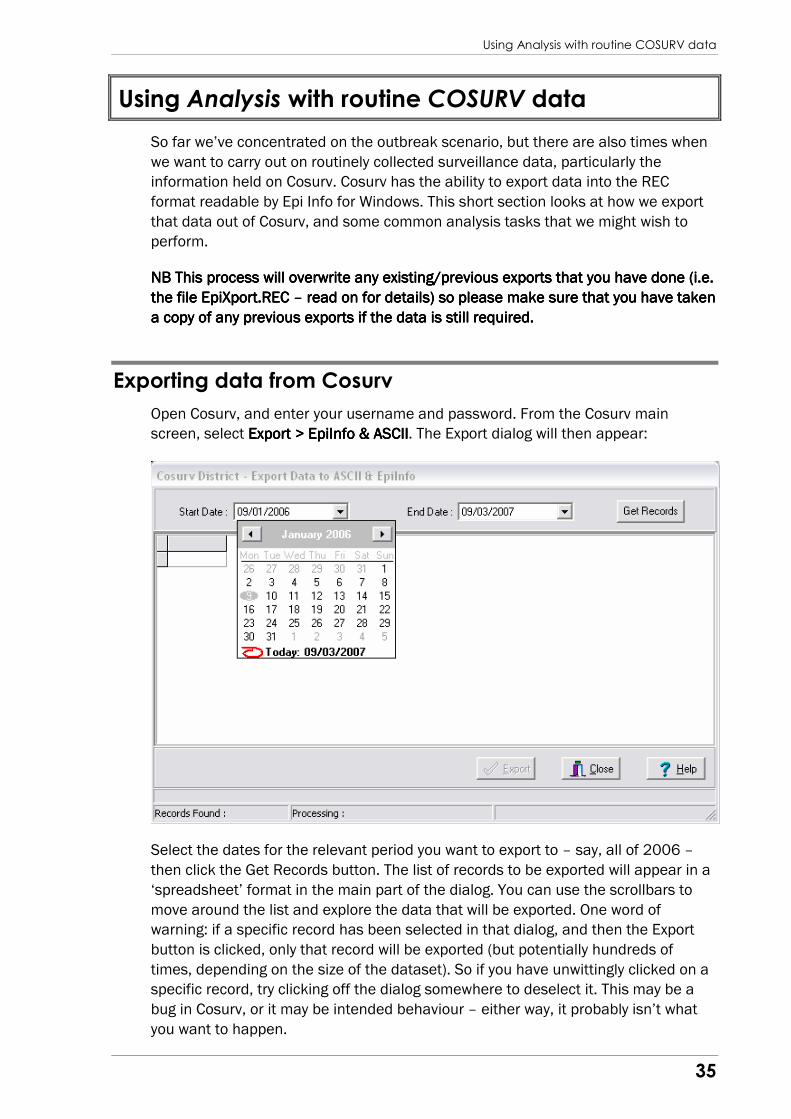
perform.
NB This process will overwrite any existing/previous exports that you have done (i.e. NB This process will overwrite any existing/previous exports that you have done (i.e. NB This process will overwrite any existing/previous exports that you have done (i.e. NB This process will overwrite any existing/previous exports that you have done (i.e.
the file EpiXport.REC the file EpiXport.REC the file EpiXport.REC the file EpiXport.REC –––– read on for details) so please make sure that you ha read on for details) so please make sure that you ha read on for details) so please make sure that you ha read on for details) so please make sure that you have taken ve taken ve taken ve taken
a copy of any previous exports if the data is still required.a copy of any previous exports if the data is still required.a copy of any previous exports if the data is still required.a copy of any previous exports if the data is still required.
Exporting data from Cosurv
Open Cosurv, and enter your username and password. From the Cosurv main
screen, select Export > EpiInfo & ASCIIExport > EpiInfo & ASCIIExport > EpiInfo & ASCIIExport > EpiInfo & ASCII. The Export dialog will then appear:
Select the dates for the relevant period you want to export to – say, all of 2006 –
then click the Get Records button. The list of records to be exported will appear in a
‘spreadsheet’ format in the main part of the dialog. You can use the scrollbars to
move around the list and explore the data that will be exported. One word of
warning: if a specific record has been selected in that dialog, and then the Export
button is clicked, only that record will be exported (but potentially hundreds of
times, depending on the size of the dataset). So if you have unwittingly clicked on a
specific record, try clicking off the dialog somewhere to deselect it. This may be a
bug in Cosurv, or it may be intended behaviour – either way, it probably isn’t what
you want to happen.
Using Analysis with routine COSURV data
36
If you’re happy with the list that’s shown, click the Export button. Cosurv will process
the export – you may see a DOS program window pop up briefly, as Cosurv actually
uses one of the old Epi Info 6 DOS utilities to carry out the export. Once the export
has been processed, you’ll be returned to the main Cosurv screen.
The exported data has been placed into an Epi Info REC file named EpiXport.REC
(NB the data has also been exported in ASCII delimited text format in a file named
csExport.txt – a format suitable for import into spreadsheet software such as Excel).
But where is it? The location of this file depends on your current Cosurv settings.
You can find these out from the main Cosurv screen by selecting System > Setup > System > Setup > System > Setup > System > Setup >
DistrictDistrictDistrictDistrict, which brings up the District settings dialog.
The final box on the General tab shows the location for Epi Info export files. When
you’ve done an export, it’s strongly recommended that you move or rename this file
appropriately to stop it being overwritten by future exports.
The data that you’re provided with for this training has been anonymised, with key
patient-identifying data (names, address, telephone numbers, employer details, id
numbers etc removed). Obviously when working with live data these will be
available, and this is something to bear in mind since it is important that data
protection and confidentiality guidelines are followed. The Cosurv data system itself
is encrypted, i.e. data can only be accessed through the password-protected Cosurv
database itself – anyone trying to access the datafiles via other methods will just
read encrypted gobbledegook. However, data exported in Epi Info (or ASCII text)
format is not encrypted, and can be read by anyone with a text editor or
spreadsheet. Therefore, you need to keep careful control over how exported data is
stored and manipulated.
Using Analysis with routine COSURV data
37
Importing data into Epi Info
Since the data is now in the REC file format, importing the data into an Epi Info
project follows the same process as discussed earlier in relation to the outbreak
data. In reality, you might want to create a separate new Epi Info project for this
routine data, but for the purposes of this training, we’ll use the same project that
we’ve been working with so far. So use the READ command in Epi Info Analysis,
select Epi6 from the Data Formats dropdown list, and then browse to select the
Cosurv2005.REC data file. Click OK to import the data into Epi Info Analysis.
Common analysis tasks for routine surveillance data
Let’s briefly look at some of the common analysis tasks that we might want to
complete with the Cosurv data. Of course, Cosurv itself has its own reporting
mechanisms through the District Reports section, but these apply only to certain
predetermined formats – using Epi Info allows us full control over the data and its
presentation. The data supplied is the anonymised surveillance reports held by
Cardiff Council for the calendar year 2005.
First of all, let’s generate some basic frequencies. Click the Frequencies command
and include the following fields in the dialog:
SEX Gender of the case
LOCALITY Locality (in Cardiff, we use electoral ward)
DISEASE Disease (as used in NOIDS return)
TRANSMISS Suspected mode of transmission
CONTRACTED Suspected source – home, commercial, unknown
The usual list of frequency tables will appear. You may or may not be surprised by
the results!
It might also be interesting to study the distribution of cases by age in the
population. Age data is stored in two ways in the Cosurv data system – the DOB
field (date of birth), and the combination of the fields AGEY (age in years) and AGEM
(months passed of current year) – so a case aged 18 months at the time of the data
entry would have AGEY=1, AGEM=6. We saw before that age has such a wide range
of values that it is often easier to recode age information into age groups for
analysis.
Let us reuse the program we created earlier in the outbreak analysis. Load the
program into the Program Editor using the Open button. We need to make one
minor modification – the variable we use for age is AGEY, whereas in the program it
refers to AGE – make any necessary modifications and then run the program. Now
run FREQ AGEGROUP to see the distribution of cases by age group (equally, we
could use this variable to construct a bar graph, or even a population pyramid by
stratifying by gender).

Using Analysis with routine COSURV data
38
We’ll now focus a bit more on the data that specifically relates to cases of Food
Poisoning. To do this we need to select only those cases where DISEASE=”Food
Poisoning”. Click the SELECT command and pick the DISEASE variable from the
dropdown list, then type =”Food Poisoning” into the dialog after the variable
name. (Alternatively, you can use the DISCODE variable and type =22, which achieves
the same thing and is quicker and easier to finish – but of course you have to know
that the DISCODE for Food Poisoning is 22).
Now lets look at the various types of organism that have been associated with
cases of food poisoning – so run a Frequencies command for the ORGANISM field.
You’ll note that organisms such as Campylobacter are basically caught under one
field, but because most isolates of Salmonella are sent to HPA Colindale for further
typing, the full breakdown of species is available for these cases.
As a final exercise, let’s investigate seasonal variation in notification of food
poisoning cases. Select the Graph command, and choose the LINE graph type.
Select the WEEK field as the main variable for the x-axis (WEEK is the NOIDS week
during which the case was notified), and leave the other default settings as they
are, since what we are looking for is the count of cases in each week. The graph will
be produced (and as before, you can continue to tinker with the display settings,
titles etc). The line is quite jagged, because there is inevitably some variation from
week to week anyway – if you wanted to ‘flatten’ this out a bit, you could produce a
similar graph in HISTOGRAM type, with an INTERVAL of either 2 or 4 weeks to
aggregate the data a bit closer (fortnightly figures are quite useful).
What What What What factors factors factors factors might explain somight explain somight explain somight explain some of the variation noted?me of the variation noted?me of the variation noted?me of the variation noted?
This training guide has introduced the basic analysis commands available in Epi
Info Analysis, with particular reference to the common epidemiological tasks
undertaken in outbreak investigation. Epi Info Analysis is a very powerful tool, and
we have only scratched the surface of the various options available, not to mention
the advanced statistical analysis that is possible. If you want to know more, a good
starting point is the further information and resources detailed in Appendix III.
Other capabilities of EpiData and Epi Info
39
Other capabilities of EpiData and Epi Info
EpiData
EpiData includes a number of additional capabilities that have not been covered in
this training guide. Some of these functions are discussed briefly below – for more
information, consult the excellent documentation in the EpiData help file.
Revise an existing questionnaire/data file
In the training, we produced a new questionnaire and REC file from scratch, in one
session. In reality, you may well design a questionnaire, pilot it with a few
individuals, and then come back and amend the questionnaire based on the
outcome of the pilot. EpiData allows you to amend an existing QES and REC file
structure. Data already entered will be copied to the new format for fields with the
same name. You can add fields, change definition of fields or delete fields. Use the
function Revise File found in the Tools menu from the main screen (close all files
first). Full instructions on how to do this are in the EpiData help file.
WARNING: If you remove fields or change the names of the fields (e.g. by changing
the text to the left of the fields) you will lose data. Please check the new, revised
data file carefully. If something goes wrong, the original data file can be restored.
The original data file is saved with the name FILENAME.OLD.REC in the same
directory as the new data file.
This ability to revise existing structures also means that it is possible to create a
‘template’ questionnaire and data file (with check code if desired) for investigation
of outbreaks. Design the basic structure once (much as we did in the training),
including patient details, medical information on illness and symptoms, details of
contacts, and so on. Create the REC file and any check code that you want to
include. When a new outbreak occurs, you can use this template as a basis by
copying and pasting all the relevant files into a new folder (so that you don’t
overwrite your ‘master template’). Then all you need to do is revise the
questionnaire to include the specific exposures that are of interest in the particular
situation, update the REC file, and you have a new questionnaire and data file
structure ready to start working with. This sort of preparation work can be valuable
in saving time in the pressured situation of a major outbreak.
Creating encrypted fields
One of the options for text fields in EpiData is the ‘Encrypted’ field (denotes in a QES
file by the notation <E >, with the total length including spaces determining
the field size). Encrypted fields are a special kind of text fields. The contents of
encrypted fields are shown in readable form on the screen, but saved on disk with
encryption. Use encrypted fields to store data in a protected mode, e.g. personal
information. When a datafile is created and the QES-file contains one or more
Other capabilities of EpiData and Epi Info
40
encrypted fields, EpiData will prompt for a password that is saved in the datafile. A
datafile containing encrypted fields can only be opened if the proper password is
entered. There is no way of breaking the encryption, so do not forget the password
or the information in that field is lost.
Data file documentation
EpiData can automatically produce a file documenting the structure and checks in
place for a particular REC file. Select Document > File StructureDocument > File StructureDocument > File StructureDocument > File Structure and then choose
the REC file you want to document in the dialog box. EpiData then produces a text
file detailing the file structure, field types and checks in place. This can then be
saved (EpiData saves these files with the .NOT extension).
Data entry notes
During data entry in EpiData of a questionnaire it is often useful to make notes (e.g.
if a difficult to read word is written on a questionnaire). The Data Entry Notes
function can be used for making short notes either during data entry or when no
data file is open.
During data entry the notes can be accessed by pressing [F8]. If no note file exists
for the current data file, a new file will be created. Current time and date are
automatically inserted in the notes.
Logical consistency check
Consistency checks are a special type of check code – rather than being associated
with a particular field, they appear in a separate block (and can even be a separate
text file), and are run by selecting Document > Consistency CheckDocument > Consistency CheckDocument > Consistency CheckDocument > Consistency Check. It provides
’batch’ checking as opposed to the interactive (i.e. as data is entered) checking that
is also offered by check commands. A number of consistency checks may be
defined in the check file or another text file. The function will show a list of all
records in the data file that fail one of the specified consistency checks.
Consistency checks are particularly useful where some data has already been
entered before interactive checks were added to the data file, and so you want to
check the existing data for consistency as well as any future records that may be
added.
Double entry and validation
To ensure a high quality of data, often it is a good strategy to have two different
persons enter the same data. In EpiData this can be done in two different ways:
either by entering the same data in two separate data files, which later can be
compared or by entering in double entry mode where the new data immediately are
compared with the original data. Detailed instructions on these processes are
available in the EpiData help file.
Other capabilities of EpiData and Epi Info
41
Data backup and encryption
EpiData has a simple data backup option – select Export Data > Export Data > Export Data > Export Data > BackupBackupBackupBackup, choose a
data file to backup and select a destination directory. Press OK to begin the backup.
This function creates a copy of the selected data file, a .QES file of the same name,
a check file of the same name and a data entry notes file of the same name in the
selected destination directory.
As an alternative to a plain backup which simply copies the files, you can compact
files and complete directory structures with the archive command in the tools
menu. This will save files in a Zip formatted file (which can be handled by other
programs e.g. WinZip, Windows Explorer on Windows XP machines). As an option
these archives can be encrypted using “strong encryption” made with the
AES/Rijndael algorithm. There is no way to find or guess a forgotten password, so
make sure you keep a copy in a safe place.
EpiData Analysis
EpiData also comes with a separate Analysis module, which is based on the
Analysis module in Epi Info 6 for DOS. Many of the commands are the same as
those used in Epi Info for Windows. In the author’s opinion, the Epi Info Analysis is
easier to use and more powerful than EpiData Analysis, which is why that software
was used for this training. However, the EpiData Analysis module is a relatively
small file, and can be installed on a PC without administrator privileges – it also
does not require a particularly high-specification of PC hardware. The final
advantage is that both EpiData and EpiData Analysis can be installed and run from
a USB stick, since they do not rely on any specific Windows libraries. The EpiData
Analysis installation file is included on the course CD-ROM.
Epi Info for Windows
In addition to the questionnaire creation, data entry and Analysis modules, Epi Info
for Windows includes several other modules and functions that may be of interest.
Again, a summary is given below, with further information available in the Epi Info
help file (see also the resources listed in Appendix III).
Map creation
Clicking Create Maps on the main Epi Info window opens the Epi Map module. Epi
Map is designed to show data from Epi Info files by relating data fields to shapefiles
containing the geographic boundaries. Shapefiles are an industry standard for
Geographic Information Systems (GIS) used in the popular ArcView and ArcInfo
programs. Shapefiles of every country in the world can be downloaded from the Epi
Info website under “Maps”, and the Internet provides thousands of such files.
Shapefiles can be drawn or edited in either ArcView or Epi Info for emergency or
custom purposes. Shapefiles also can contain data on population or other
variables, and can therefore provide numeric data that become part of the display
either as numerator or denominator. Numeric data can be displayed either as
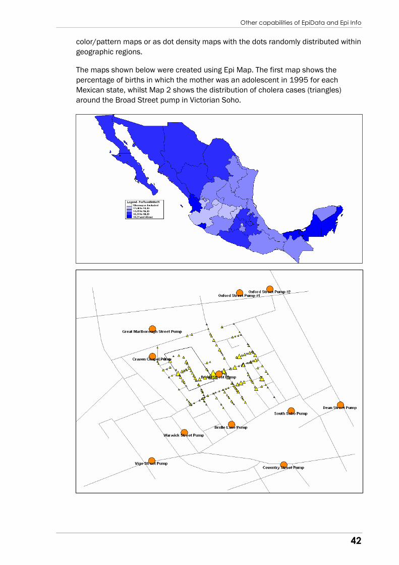
Other capabilities of EpiData and Epi Info
42
color/pattern maps or as dot density maps with the dots randomly distributed within
geographic regions.
The maps shown below were created using Epi Map. The first map shows the
percentage of births in which the mother was an adolescent in 1995 for each
Mexican state, whilst Map 2 shows the distribution of cholera cases (triangles)
around the Broad Street pump in Victorian Soho.

Other capabilities of EpiData and Epi Info
43
An excellent tutorial on using Epi Map to present geographical data in a visual
format can be found in Andrew Dean’s Introduction to Epi Info for Windows,
available at http://www.epiinformatics.com/Resources.htm.
StatCalc – a simple epidemiological calculator
StatCalc is an epidemiologic calculator the produces statistics from summary data
entered on the screen – particularly useful when you only have the summary data
available (and so the conventional tools in Epi Info Analysis are not suitable). Three
types of calculations are offered:
♦ Statistics for 2-by-2 and 2-by-n tables
♦ Sample Size Calculations
♦ Chi Square for Trend
You can access StatCalc from the main Epi Info menu, by selecting Utilities > Utilities > Utilities > Utilities >
StatCalcStatCalcStatCalcStatCalc.
Producing reports of analysis results
Clicking Create Reports opens the Epi Reports module. The Epi Report tool can be
used to design and generate various reports. An end user can include various
elements in the reports generated, and these elements can be bound to various
data sources. Record lists, cell replacement, groups, fragments from analysis XML
can be included in the report. Data analysis through pivot table is also provided.
Read the Epi Info help file for more details, and see also the CDC Epi Info Exercises
file, which is included on the CD-ROM with the installation files – one of the
chapters in this file deals with using Epi Reports.
Encrypting Epi Info Projects
Epi Lock provides encryption to control access to data files and compression to
facilitate both transmission and making backup copies. Using Epi Lock, files can be
encrypted with a password to reduce the risk of others being able to read the data.
The encryption mechanism also provides some assurance that the files have not
been altered in transmission, since they will not decrypt properly if altered. Epi Lock
also performs the function of properly deleting the unencrypted version (“clear
text”) version of the file after testing to make sure that the encrypted version can be
decrypted to produce the identical result. Access the Epi Lock functions by selecting
Utilities > Epi LockUtilities > Epi LockUtilities > Epi LockUtilities > Epi Lock from the main Epi Info menu.

Appendix I – Comparison of Epi Info & EpiData
44
Appendix I – Comparison of Epi Info & EpiData
This article was published in Eurosurveillance Weekly Release surveillance report
(vol 12, issue 1, 12 January 2007). The original can be accessed online at:
♦ http://www.eurosurveillance.org/ew/2007/070111.asp#4
A comparison of public domain software for outbreak
investigations: Epi Info and EpiData
G Kafatos ([email protected]), NQ Verlander, D Gelb, E Arnold, A Charlett
Statistics, Modelling and Bioinformatics Department, Health Protection Agency
Centre for Infections, London, UK
Since the early 1980s, there has been an increase in the number of outbreaks
investigated using analytical epidemiology since it became widely accepted that
microbiological investigation alone is often insufficient [1, 2, 3]. This increase has also
been encouraged by a growing availability of statistical tools within public health
and the establishment of international and national training programmes and
courses (such as the European Programme for Intervention Epidemiology Training).
In 1985, a team at the Centers for Disease Control and Prevention (CDC) in the
United States created a suite of public domain computer programs called Epi Info
(http://www.cdc.gov/epiinfo/), which were designed to support field
epidemiological investigations of outbreaks.
We compare the two most recent versions of Epi Info, and EpiData, a public domain
software based on Epi Info 6.04d.
Epi Info 6.04d
Since the release of its first version written for the DOS-environment in 1986, Epi
Info quickly became very popular amongst epidemiologists and other public health
professionals. Its popularity is demonstrated by the fact that the program is
available in 16 different languages. In 2001, the CDC released the final version of
Epi Info DOS (Epi Info 6.04d).
Epi Info DOS consists of a suite of programs, which provide all that is necessary to
support an outbreak investigation. It is a flexible, versatile tool that permits the
construction of a data entry system and an underlying database with great speed,
which is something greatly appreciated under the time pressures of an on-going
outbreak investigation.
In addition, Epi Info DOS contains an analysis module for elementary statistical
analysis that is very useful for outbreak investigations where the outcome is often
binary (case/control, ill/not ill). The ‘tables’ command provides all the necessary
measures of the strength of association, such as odds ratios (OR) and risk ratios
(RR), their confidence intervals, and hypothesis tests. It also allows stratified
Appendix I – Comparison of Epi Info & EpiData
45
analysis to remove the effects of up to three confounding factors. The ‘csample’
module enables cluster analysis and stratified designed surveys. Epi Info DOS was
complemented by a CDC public domain mapping software (Epi Map, CDC), allowing
area maps to be produced directly from Epi Info files.
Epi Info for Windows 3.3.2
Despite the unprecedented success of Epi Info DOS, by the late 1990s, the
widespread uptake of the Microsoft Windows operating system for personal
computers meant that a Windows version was needed. Epi Info 2000 (Epi Info 3) for
Windows was released in 2000. However, there are substantial differences
compared with Epi Info DOS.
The analysis capability of Epi Info DOS was carried forward to Epi Info 3 while
adding the ability to estimate proportional hazards models and integrating logistic
regression and mapping facilities into the package. The software uses components
from commercial software, which enhances its compatibility with ‘industry
standards’ such as Microsoft Office Access 2003. However, this is also the main
disadvantage, since it has resulted in the loss of some functions (such as copying
and pasting of fields in questionnaire creation and of check commands between
different fields) reducing the speed of usage, a key requisite for outbreak
investigations. Moreover, because the principle of simplicity and easy use which
underpinned the creation of Epi Info DOS was not carried forward to Epi Info 3,
those who have worked with Epi Info DOS will need training to become proficient
users of Epi Info 3.
EpiData 3.1 (120306)
EpiData was initially released in 2000 by a non-profit organisation in Denmark
(EpiData Association, http://www.epidata.dk/). The current version 3.1 became
available in 2006. This software was developed specifically to translate Epi Info
DOS into Windows software by using the Epi Info DOS file structures and command
language wherever possible.
Certain restrictions in file size were removed but those dependent upon file
structures remain. Construction of a data entry system using EpiData is very simple,
especially if the original questionnaire has been constructed in a Windows-based
word processing software where it can be either opened as a text file or copied
directly into EpiData.
For validating double-entered data (a common practice to ensure high quality data)
the ‘Validate Duplicate Files’ option in EpiData has built on the dual entry validation
capability within Epi Info DOS. Two additional options to either ‘Ignore text fields’ or
‘Ignore letter-case in text fields’ resolve the problems that occur when comparing
text fields (i.e. two identical text fields are considered different by the software if
one is written in capital and the other in lower-case letters).

Appendix I – Comparison of Epi Info & EpiData
46
EpiData Analysis (v1.1 Build 68)
When EpiData was originally released, one major disadvantage was its lack of
analytical statistical tools. This was addressed with the introduction of EpiData
Analysis in 2005. This provides the statistical methods available within the analysis
module of Epi Info DOS, but has greatly improved data manipulation facilities.
A wide range of statistical tools exists within Epi Data Analysis, including analysis of
variance, which provides a t-test for independent groups, chi-square and Fisher’s
exact tests of association, nonparametric tests of difference in location between
two groups, and estimates of measures of association with confidence intervals.
The graphical capability in EpiData Analysis is much better than Epi Info DOS, with
more options and flexibility. While the graphs are acceptable for descriptive
purposes, there will probably always be limitations in producing publication quality
graphs. A new capability within EpiData Analysis is the ability to produce statistical
process control (SPC) charts for performance monitoring applicable for surveillance
data.
Discussion
Two public domain software packages have been developed based on the classic
DOS version of Epi Info. There does seem to be a divergence in the development of
EpiData (Entry and Analysis) and Epi Info 3, which is surprising given their common
ancestor, Epi Info DOS. While EpiData has aimed to keep the functionality and
interface of Epi Info DOS available, Epi Info 3 appears to be developing into a more
general software to support epidemiologists rather than keeping with the original
concept of an efficient and relatively simple software for outbreak investigation.
It is difficult to decide which of the two development directions will best meet the
needs of epidemiologists over the next twenty years. It is possible that there is a
place for both. The DOS version of Epi Info was extremely well-structured and
efficient and, as EpiData has remained faithful to this concept, this could be seen
as its natural successor. With the requirement for more sophisticated analytical
methods to overcome issues such as confounding, it may be that Epi Info 3 will be
better placed. However, it is now moving into a very competitive arena where
commercial software has predominated. The authors would recommend EpiData
3.1 and EpiData Analysis v1.1 software packages for those involved in the
investigation of infectious disease outbreaks for their speed and simplicity of use in
a Windows environment.
Reviewed software:
Epi Info, version 6.04d for DOS and version 3.3.2 for Windows
Centers for Disease Control and Prevention (CDC), Atlanta, Georgia 30333.
Can be downloaded from www.cdc.gov/epiinfo/Epi6/ei6.htm (DOS) and
www.cdc.gov/epiinfo/ (Windows)
EpiData, version 3.1 (120306) and EpiData Analysis, version 1.1 Build 68

Appendix I – Comparison of Epi Info & EpiData
47
The EpiData Association, att. Jens Lauritsen, Enghavevej 34, DK5230 Odense
M, Denmark. Can be downloaded from www.epidata.dk/download.php
References:
1. Fonseca MGP & Armenian HK (1991) Use of the Case-Control Method in
Outbreak Investigations. American Journal of Epidemiology 133: 748-752
2. O'Brien SJ, Elson R, Gillespie IA, Adak GK, & Cowden JM (2002). Surveillance
of foodborne outbreaks of infectious intestinal disease in England and Wales
1992-1999: contributing to evidence-based food policy? Public Health 116:
75-80
3. Palmer SR (1989) Epidemiology in search of infectious diseases: methods in
outbreak investigation. Journal of Epidemiology and Community Health 43:
311-314

Appendix II – Contents of course CD-ROM
48
Appendix II – Contents of course CD-ROM
♦ This training guide (Adobe PDF document)
♦ Examples of files that might be produced by following this training:
◊ AGEGROUPS.PGM – sample analysis program file for recoding age into
agegroups
◊ Completed worksheet for 2x2 table results (Adobe PDF document) – see
Appendix IV
◊ Lead Officer.CHK – EpiData check code file
◊ Lead Officer.MDB – Epi Info project
◊ Lead Officer.QES – EpiData questionnaire file
◊ Lead Officer.REC – EpiData data file
♦ Installation and support files:
◊ EpiData Setup
◊ EpiData Analysis Setup
◊ Epi Info Setup
◊ CDC Epi Info Exercises (Word document)
◊ OpenEpi project (Zip archive file) – see Appendix III
Appendix III – Further information & resources
49
Appendix III – Further information & resources
EpiData
EpiData homepage
http://www.epidata.dk/
EpiData email discussion list
http://lists.umanitoba.ca/mailman/listinfo/epidata-list
List intended for discussions, suggestions and help among users of EpiData.
EpiData documentation and technical info
http://www.epidata.dk/documentation.php
Extended manuals, field notes and technical information on use of EpiData, as
well as some general guidance on data management.
EpiData Wiki
http://www.epidata.org/wiki
Common entry for development of field guides, questions and solutions. All
users can add their suggestions and knowledge to the site. A couple of useful
field guides already exist, including one on the investigation of a food
poisoning outbreak.
Epi Info
Centers for Disease Control & Prevention: Epi Info homepage
http://www.cdc.gov/epiinfo
CDC Epi Info Tutorials
http://www.cdc.gov/epiinfo/tutorials.htm
Two tutorials designed and published by CDC – one based on a cholera
outbreak, and the other on a community health assessment.

Appendix III – Further information & resources
50
Epi Informatics - Dr Andrew Dean
http://www.epiinformatics.com/
Site dedicated to the use of computers in epidemiology and public health.
Includes a brief online introduction to Epi Info, and links to download a more
complete introductory manual, together with two 15-hour courses (complete
with tutor manuals).
Professor Kevin Sullivan
http://www.sph.emory.edu/~cdckms/
Includes tutorials on Epi Info for Windows and Epi Info 6 for DOS, as well as
general epidemiology documents.
http://www.google.co.uk/
The above sites are just a summary – there is a wide range of training
materials, courses etc. relating to Epi Info available globally – a simple Google
search on ‘Epi Info training’, ‘Epi Info exercises’, ‘Epi Info
tutorials’ etc. should give a good range of resources.
Epidemiology and Statistics
CDC General Training Resources
http://www.cdc.gov/descd/materials.html#foodborne
In addition to the cholera outbreak tutorial referred to above, three other
epidemiologic case studies that focus on real-life food borne disease outbreak
investigations. Not specifically based on Epi Info.
OpenEpi
http://www.openepi.com/
OpenEpi is a project to create open source software for Epidemiologic
statistics in JavaScript and HTML. OpenEpi can be run from a web site or
downloaded and run without a web connection. The OpenEpi files are also
included on the course CD-ROM for installation and use without the need for
internet access.
Epidemiology Supercourse
http://www.pitt.edu/~super1/index.htm
The Supercourse is a global repository of lectures on public health and
prevention targeting educators across the world. Supercourse has a network
of over 41300 scientists in 171 countries who are sharing a free library of
over 3162 lectures in 26 languages.
Appendix III – Further information & resources
51
StatPages
http://www.statpages.org/
Index of web pages that together comprise a powerful, conveniently
accessible, multi-platform statistical software package. There are also links to
online statistics books, tutorials, downloadable software, and related
resources.
Rice Virtual Lab in Statistics
http://www.onlinestatbook.com/rvls.html
Online statistics book with simulations/demonstrations, case studies, and online
analysis tools.
Outbreak Investigations – A Perspective
http://www.cdc.gov/ncidod/EID/vol4no1/reingold.htm
Article from the peer-reviewed journal Emerging Infectious Diseases that
provides an excellent overview of the principles of outbreak investigation and
the issues involved.
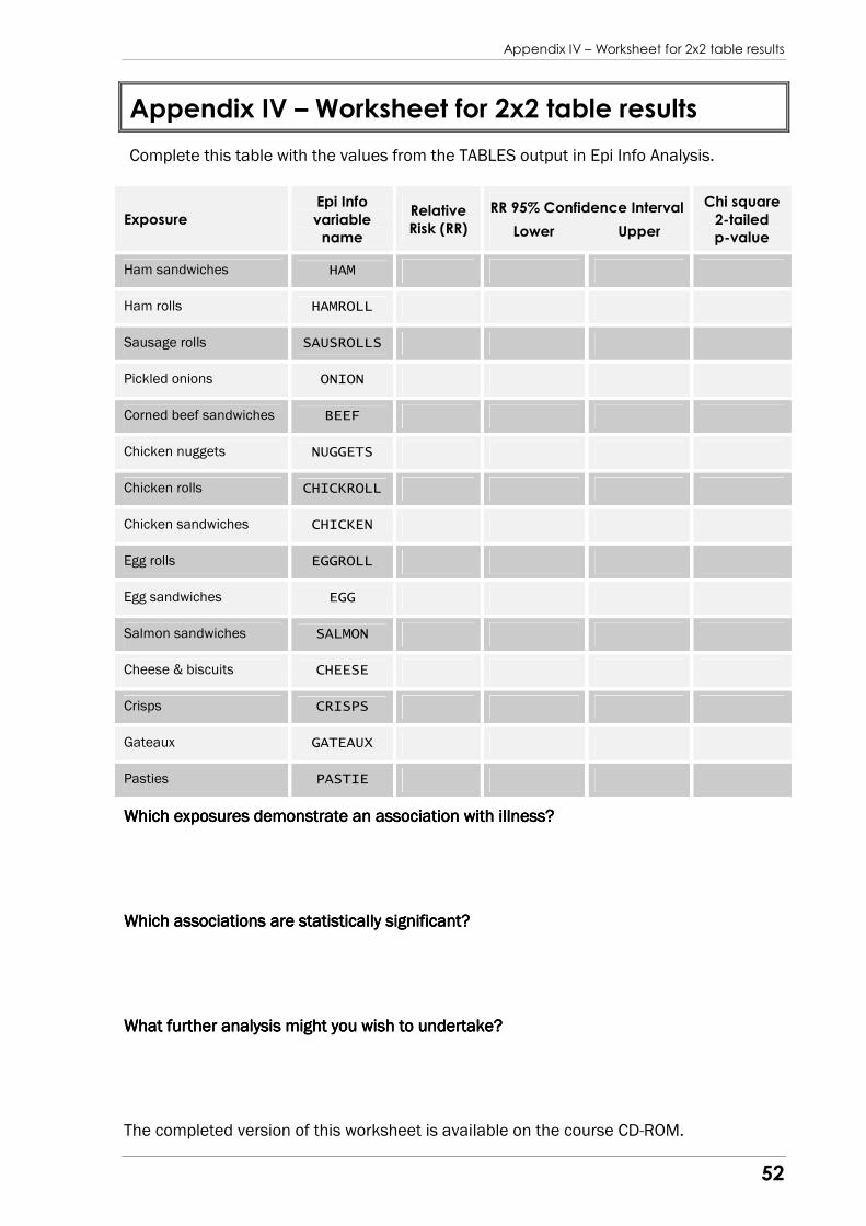
Appendix IV – Worksheet for 2x2 table results
52
Appendix IV – Worksheet for 2x2 table results
Complete this table with the values from the TABLES output in Epi Info Analysis.
Which exposures demonstrate an association with illness?Which exposures demonstrate an association with illness?Which exposures demonstrate an association with illness?Which exposures demonstrate an association with illness?
Which associations aWhich associations aWhich associations aWhich associations are statistically significant?re statistically significant?re statistically significant?re statistically significant?
What further analysis might you wish to undertake?What further analysis might you wish to undertake?What further analysis might you wish to undertake?What further analysis might you wish to undertake?
The completed version of this worksheet is available on the course CD-ROM.
Exposure
Epi Info
variable
name
Relative
Risk (RR)
RR 95% Confidence Interval
Lower Upper
Chi square
2-tailed
p-value
Ham sandwiches HAM
Ham rolls HAMROLL
Sausage rolls SAUSROLLS
Pickled onions ONION
Corned beef sandwiches BEEF
Chicken nuggets NUGGETS
Chicken rolls CHICKROLL
Chicken sandwiches CHICKEN
Egg rolls EGGROLL
Egg sandwiches EGG
Salmon sandwiches SALMON
Cheese & biscuits CHEESE
Crisps CRISPS
Gateaux GATEAUX
Pasties PASTIE
Appendix V – Check code example
53
Appendix V – Check code example
Calculating incubation period
It would often be useful to be able to calculate the incubation period to assist with
producing an epidemic curve. In the examples we followed in the analysis training,
this data was given to us – but if this was calculated ‘manually’, it introduces the
possibility of human calculation or data entry errors. Far easier to have the period
calculated for us at the time of data entry, based on the onset date and time
reported. We would also need to set an arbitrary ‘base date’ – which could be the
date of an implicated event, or just a specific date at some point before the first
case. To keep things simple we track the period from midnight on the ‘base date’
In the following examples it is assumed that the fields ONSETDATE and ONSETTIME
refer to the actual date and time reported by the case. The field INCUBATION is a
numeric field (say, two or three digits long with no decimal places) that will hold the
calculated values (whether in hours or days). You may need to modify the check
code examples to reflect the fieldnames that you have used.
Where the illness in question has a relatively long incubation period, likely to be
measured in days (as might be the case in e.g. typhoid, Cryptosporidium, Legionella
outbreaks), this is a simple matter of deducting the ‘base date’ from the ‘onset
date’ to obtain the period in days. The int function is used to convert the answer
into a numeric value to match the INCUBATION field). The check code for this would
appear in relation to the ONSETDATE field, and would read something like the
following:
AFTER ENTRY DEFINE basedate <dd/mm/yyyy> basedate = “14/08/1998” INCUBATION = int(ONSETDATE – basedate) END
The situation gets a little more complicated where a shorter incubation period is
suggested, such as might be the case with many ‘food poisoning’ organisms such
as Salmonella spp., Clostridium perfringens, Bacillus cereus etc. Since EpiData
stores date and time details in separate fields, a more complex calculation is
required. The check code would need to appear in relation to whichever of
ONSETDATE and ONSETTIME was last on the questionnaire (and therefore last to have
data entered). The calculation would look something like this:
AFTER ENTRY DEFINE basedate <dd/mm/yyyy> basedate = “14/08/1998” INCUBATION=(int(ONSETDATE-basedate)*24) + trunc(ONSETTIME) END
This code initially looks the same, in that the first part of the main calculation
determines the difference in days between the base date and onset date. This value
(in days) is then multiplied by 24 to convert it into hours. Finally, we include the
Appendix V – Check code example
54
onset time element by simply adding the value in hours on (to keep things simple,
we limit the value to hours by truncating the time field to the hour, ignoring the
minutes).
Further tinkering with the time element of the calculation allows you to set a base
time to go with the base date, which could be of use where a specific event is
implicated. This involves defining a ‘base time’ using the 24-hour clock, and
deducting that number of hours from the calculation formula above (since that
formula is based on time passed since midnight, so any other base time will reduce
the incubation period accordingly). The check code would then look like this:
AFTER ENTRY DEFINE basedate <dd/mm/yyyy> basedate = “14/08/1998” DEFINE basetime ##.## basetime = 15.00 INCUBATION=((int(ONSETDATE-basedate)*24) + trunc(ONSETTIME)) –
trunc(basetime) END