Environmental Impact Report windmill farm Rentel transport...Rentel NV Environmental Impact Report...

Rentel NV

Environmental Impact Report windmill farm Rentel

Numeric modelling of sediment transport

25 June 2012 - version 2.0

Colophon

International Marine & Dredging Consultants

Address: Coveliersstraat 15, 2600 Antwerp, Belgium

: + 32 3 270 92 95

: + 32 3 235 67 11

Email: [email protected]

Website: www.imdc.be

IMDC nv Windmill farm Rentel Sediment transport modelling

I/RA/11397/12.072/LWA 4 version 2.0 - 25/06/12

Table of Contents

1. INTRODUCTION ................................................................................................................... 8

1.1 THE ASSIGNMENT ........................................................................................................... 8

1.2 AIM OF THE STUDY ......................................................................................................... 8

1.3 OVERVIEW OF THE STUDY ............................................................................................ 9

1.4 STRUCTURE OF THE REPORT ....................................................................................... 9

2. DESCRIPTION OF NUMERICAL MODEL ......................................................................... 10

2.1 HYDRODYNAMIC FLOW MODEL .......................................................................................... 10

2.1.1 Numerical grid and bathymetry ............................................................................... 10

2.1.2 Boundary conditions ............................................................................................... 12

2.1.3 Validation ................................................................................................................ 15

2.2 WAVE MODEL ................................................................................................................... 18

2.2.1 Introduction ............................................................................................................. 18

2.2.2 Numerical grid and bathymetry ............................................................................... 19

2.2.3 Boundary conditions ............................................................................................... 20

2.2.4 Validation ................................................................................................................ 23

2.3 SEDIMENT TRANSPORT MODEL............................................................................................ 26

2.3.1 Boundary conditions and median grainsize ............................................................ 26

3. RESULTS ............................................................................................................................ 28

3.1 SUMMER CONDITION (TIDAL CURRENTS ONLY) ..................................................................... 28

3.1.1 Currents .................................................................................................................. 28

3.1.2 Bottom shear stress ................................................................................................ 32

3.1.3 Sediment transport and morphological evolution ................................................... 34

3.2 WINTER CONDITION (TIDES + WAVES) ............................................................................... 36

3.2.1 Currents and waves ................................................................................................ 36

3.2.2 Bottom shear stress ................................................................................................ 40

3.2.3 Sediment transport and morphological evolution ................................................... 41

4. DISCUSSION ...................................................................................................................... 43

5. CONCLUSIONS .................................................................................................................. 46

6. REFERENCES .................................................................................................................... 47


I/RA/11397/12.072/LWA 5 version 2.0 - 25/06/12

List of Tables

TABLE 1 VALUES OF AVERAGED TIDAL RANGE OF THE SELECTED REPRESENTATIVE TIDAL PERIOD

AND ANNUAL MEAN TIDAL RANGE AT THREE STATIONS .............................................................. 13

List of Figures

FIGURE 2-1 LAYOUT OF THE MODEL GRIDS ...................................................................................... 10

FIGURE 2-2 THREE DOMAINS AFTER DOMAIN DECOMPOSITION .......................................................... 11

FIGURE 2-3 BATHYMETRY MAP OF THE FLOW MODEL DOMAIN ........................................................... 11

FIGURE 2-4 LEFT PANEL: THREE-DIMENSIONAL BATHYMETRY MAP OF THE WHOLE FLOWMODEL

DOMAIN; RIGHT PANEL: THREE-DIMENSIONAL BATHYMETRY MAP OF THE RENTEL DOMAIN .......... 12

FIGURE 2-5 TIDAL GAUGES IN THE MODEL DOMAIN ........................................................................... 12

FIGURE 2-6 TIDAL RANGES AT THREE STATIONS IN 2009 .................................................................. 13

FIGURE 2-7 MOVING AVERAGED TIDAL RANGE FOR SPRING-NEAP TIDAL CYCLE AT THREE

STATIONS .............................................................................................................................. 14

FIGURE 2-8 TIDAL ELEVATION OBSERVED AT MOW0 STATION DURING THE REPRESENTATIVE

PERIOD .................................................................................................................................. 14

FIGURE 2-9 LOCATION OF OBSERVATION POINTS ............................................................................. 16

FIGURE 2-10 COMPARISON OF TIDAL ELEVATION AT WESTHINDER .................................................... 16

FIGURE 2-11 COMPARISON OF VELOCITY AT SCHEUR WIELINGEN .................................................... 17

FIGURE 2-12 COMPARISON OF VELOCITY AT LODEWIJKBANK ............................................................ 18

FIGURE 2-13 THE WAVE MODEL GRIDS (MAIN WAVE MODEL: WAVE GRID, NESTED WAVE MODEL: RENTEL DOMAIN) AND THE THREE DOMAINS OF THE FLOW MODEL ............................................ 19

FIGURE 2-14 BATHYMETRY MAP OF THE WAVE MODEL AND TWO WAVE MONITORING STATIONS .......... 20

FIGURE 2-15 SIGNIFICANT WAVE HEIGHT OBSERVED AT WESTHINDER FROM 01-JULY-1990 TO

01-JULY-2010 ....................................................................................................................... 20

FIGURE 2-16 UPPER PANELS: PERFORMANCE OF THE STATISTICAL MODEL; LOWER PANEL: CORRELATION BETWEEN VARIABLE LEVEL AND RETURN PERIOD. ............................................... 21

FIGURE 2-17 PEAKS OF THE SIGNIFICANT WAVE HEIGHT MONITORED AT WESTHINDER ....................... 22

FIGURE 2-18 WIND CONDITIONS COLLECTED AT WESTHINDER DURING THE SELECTED STORM

PERIOD .................................................................................................................................. 23

FIGURE 2-19 WAVE CONDITIONS COLLECTED AT SANDETTIE LIGHTSHIP DURING THE SELECTED

STORM PERIOD ...................................................................................................................... 23

FIGURE 2-20 ONE-ON-ONE RELATION BETWEEN THE SIGNIFICANT WAVE HEIGHT CALCULATED BY

DELFT3D-WAVE AND MEASURED AT THE WESTHINDER BUOY LOCATION .................................. 24

FIGURE 2-21 VALIDATION OF THE DELFT3D-WAVE MODEL WITH FIELD MEASUREMENTS OF THE

DIRECTIONAL WAVE BUOY AT THE WESTHINDER BANK. COMPARISON OF THE TIME SERIES

OF THE SIGNIFICANT WAVE HEIGHT HM0, THE MEAN ZERO-CROSSING WAVE PERIOD TM02 AND

WAVE DIRECTION ................................................................................................................... 25

FIGURE 2-22 MAP OF THE GRAINSIZE DISTRIBUTION (ADAPTED AFTER VERFAILLIE ET AL., 2006). THE RENTEL CONCESSION ZONE IS THE BROWN HATCHED AREA IN THE MIDDLE OF THE

FIGURE, THE DARK BLUE CONTOUR IS THE COMPUTER MODEL OF THE RENTEL AREA. ................. 27


I/RA/11397/12.072/LWA 6 version 2.0 - 25/06/12

FIGURE 3-1 BATHYMETRY MAP WITH ISOBATH CONTOUR LINES OF -25 M NAP; RED CROSS AND

TRIANGLE LABEL TWO POINTS IN THE RENTEL ZONE FOR INSPECTION OF TIME SERIES

VARIABLES ............................................................................................................................. 28

FIGURE 3-2 TIME SERIES SHOWING CURRENT VELOCITY MAGNITUDE AND TIDAL ELEVATION AT

THE RED CROSS POINT ........................................................................................................... 29

FIGURE 3-3 TIME SERIES SHOWING CURRENT VELOCITY MAGNITUDE AND TIDAL ELEVATION AT

THE RED TRIANGLE POINT ....................................................................................................... 29

FIGURE 3-4 MAP OF AVERAGED CURRENT ELLIPSES IN SUMMER CONDITIONS WITH BATHYMETRY

AS BACKGROUND; THE AVERAGED CURRENT ELLIPSES ARE CALCULATED OVER THE

REPRESENTATIVE SPRING-NEAP TIDAL CYCLE; THE GRID RESOLUTION OF ONE ELLIPSE IS

ABOUT 1000M × 500M. .......................................................................................................... 30

FIGURE 3-5 MAP OF AVERAGED CURRENT VELOCITY MAGNITUDE CALCULATED OVER THE

REPRESENTATIVE SPRING-NEAP TIDAL CYCLE IN SUMMER CONDITIONS WITH ISOBATH LINES

OF -25 M NAP ....................................................................................................................... 30

FIGURE 3-6 MAP OF MAXIMAL CURRENT VELOCITY MAGNITUDE OVER THE REPRESENTATIVE

SPRING-NEAP TIDAL CYCLE IN SUMMER CONDITIONS WITH ISOBATH LINES OF -25 M NAP ........... 31

FIGURE 3-7 MAP OF THE RESIDUAL CURRENT CALCULATED OVER THE REPRESENTATIVE SPRING-NEAP TIDAL CYCLE IN SUMMER CONDITIONS WITH RESIDUAL VELOCITY MAGNITUDE AS

BACKGROUND AND ISOBATH LINES OF -25 M NAP .................................................................... 32

FIGURE 3-8 MAP OF THE AVERAGED SHEAR STRESS MAGNITUDE CALCULATED OVER THE

REPRESENTATIVE SPRING-NEAP TIDAL CYCLE IN SUMMER CONDITION WITH ISOBATH LINES

OF -25M ................................................................................................................................ 33

FIGURE 3-9 MAP OF MAXIMAL SHEAR STRESS MAGNITUDE OVER THE REPRESENTATIVE SPRING-NEAP TIDAL CYCLE IN SUMMER CONDITION WITH ISOBATH LINES OF -25M ................................... 33

FIGURE 3-10 MAP OF RESIDUAL SEDIMENT TRANSPORT CALCULATED OVER THE

REPRESENTATIVE SPRING-NEAP TIDAL CYCLE IN SUMMER CONDITIONS WITH TRANSPORT

RATE AS BACKGROUND AND ISOBATH LINES OF -25 M ............................................................... 34

FIGURE 3-11 MAP OF SEDIMENTATION AND EROSION CALCULATED OVER THE REPRESENTATIVE

SPRING-NEAP TIDAL CYCLE IN SUMMER CONDITIONS WITH VECTORS OF RESIDUAL SEDIMENT

TRANSPORT AND ISOBATH LINES OF -25 M NAP ....................................................................... 35

FIGURE 3-12 TIME SERIES OF MODELLED SEDIMENT TRANSPORT AND VELOCITY MAGNITUDE

DURING THE REPRESENTATIVE SPRING-NEAP TIDAL CYCLE IN SUMMER CONDITIONS AT THE

RED TRIANGLE POINT .............................................................................................................. 35

FIGURE 3-13 TIME SERIES OF MODELLED SIGNIFICANT WAVE HEIGHT AND TIDAL ELEVATION

DURING THE REPRESENTATIVE SPRING-NEAP TIDAL CYCLE IN WINTER CONDITIONS AT THE


FIGURE 3-14 MAP OF AVERAGED CURRENT ELLIPSES IN WINTER CONDITIONS WITH BATHYMETRY

AS BACKGROUND; THE AVERAGED CURRENT ELLIPSES ARE CALCULATED OVER THE

REPRESENTATIVE SPRING-NEAP TIDAL CYCLE; THE GRID RESOLUTION OF ONE ELLIPSE IS

ABOUT 1000 M × 500 M .......................................................................................................... 37

FIGURE 3-15 MAP OF AVERAGED CURRENT VELOCITY MAGNITUDE CALCULATED OVER THE

REPRESENTATIVE SPRING-NEAP TIDAL CYCLE IN WINTER CONDITIONS WITH ISOBATH LINES

OF -25 M NAP ....................................................................................................................... 37

FIGURE 3-16 MAP OF MAXIMAL CURRENT VELOCITY MAGNITUDE OVER THE REPRESENTATIVE

SPRING-NEAP TIDAL CYCLE IN WINTER CONDITIONS WITH ISOBATH LINES OF -25 M NAP ............. 38

FIGURE 3-17 MAP OF RESIDUAL CURRENT CALCULATED OVER THE REPRESENTATIVE SPRING-NEAP TIDAL CYCLE IN WINTER CONDITIONS WITH RESIDUAL VELOCITY MAGNITUDE AS

BACKGROUND AND ISOBATH LINES OF -25 M NAP .................................................................... 38


I/RA/11397/12.072/LWA 7 version 2.0 - 25/06/12

FIGURE 3-18 MAP OF AVERAGED SIGNIFICANT WAVE HEIGHT CALCULATED OVER THE


OF -25 M NAP ....................................................................................................................... 39

FIGURE 3-19 MAP OF MAXIMAL SIGNIFICANT WAVE HEIGHT OVER THE REPRESENTATIVE SPRING-NEAP TIDAL CYCLE IN WINTER CONDITIONS WITH ISOBATH LINES OF -25 M NAP ......................... 39

FIGURE 3-20 MAP OF AVERAGED SHEAR STRESS MAGNITUDE CALCULATED OVER THE


OF -25 M NAP ....................................................................................................................... 40

FIGURE 3-21 MAP OF MAXIMAL SHEAR STRESS MAGNITUDE OVER THE REPRESENTATIVE SPRING-NEAP TIDAL CYCLE IN WINTER CONDITIONS WITH ISOBATH LINES OF -25 M NAP ......................... 40

FIGURE 3-22 MAP OF RESIDUAL SEDIMENT TRANSPORT CALCULATED OVER THE

REPRESENTATIVE SPRING-NEAP TIDAL CYCLE IN WINTER CONDITIONS WITH TRANSPORT

RATE AS BACKGROUND AND ISOBATH LINES OF -25 M NAP ....................................................... 41

FIGURE 3-23 MAP OF SEDIMENTATION AND EROSION CALCULATED OVER THE REPRESENTATIVE

SPRING-NEAP TIDAL CYCLE IN WINTER CONDITIONS WITH VECTORS OF RESIDUAL SEDIMENT

TRANSPORT AND ISOBATH LINES OF -25 M NAP ....................................................................... 42

FIGURE 4-1 TIME SERIES OF MODELLED SEDIMENT TRANSPORT IN SUMMER AND WINTER

CONDITIONS, AND MODELLED SIGNIFICANT WAVE HEIGHT IN WINTER CONDITIONS AT THE


FIGURE 4-2 TIME SERIES OF MODELLED SEDIMENT TRANSPORT IN SUMMER AND WINTER

CONDITIONS, AND MODELLED SIGNIFICANT WAVE HEIGHT IN WINTER CONDITIONS AT THE

RED CROSS POINT .................................................................................................................. 44

FIGURE 4-3 TIME SERIES OF MODELLED CHANGE OF SEDIMENT THICKNESS IN SUMMER AND

WINTER CONDITIONS AT THE RED TRIANGLE POINT ................................................................... 44

FIGURE 4-4 TIME SERIES OF MODELLED CHANGE OF SEDIMENT THICKNESS IN SUMMER AND

WINTER CONDITIONS AT THE RED CROSS POINT........................................................................ 45


I/RA/11397/12.072/LWA 8 version 2.0 - 25/06/12

1. INTRODUCTION

1.1 THE ASSIGNMENT

According to the Belgian legislation a concession is required for the construction and

exploitation of a windmill park. A necessary part to obtain a concession permit is the writing of

an Environmental Impact Assessment (EIA) of the foreseen activities. This task was assigned

by Rentel NV to International Marine and Dredging Consultants NV on 2nd November 2011.

The description of the initial reference situation and the possible natural evolution of the

subsurface is an important element of the EIA. In order to assess the autonomic evolution of

the seafloor a numerical model had to be set-up that simulates the tidal currents, wave action

and sediment transport in the concession area. This additional study was granted to IMDC NV

on 28 February 2012. A detailed scope of work of this particular study was set up in close

collaboration with the MUMM (Dries Van den Eynde) in order to fulfil the specific requirements

of the EIA.

The dredging and disposal methods for the construction of the windmill park will likely cause

turbidity and sediment dispersion. In order to assess the impact of the dredging activities on

the background turbidity and suspended sediment levels, a dredging plume model study was

proposed by IMDC. This additional study was granted to IMDC NV on 9 May 2012. A

numerical model will be applied that simulates the tidal currents and sediment transport in the

concession area.

1.2 AIM OF THE STUDY

In the framework of the EIA for the planned windmill park Rentel, the stability of the sandy

subsurface in the concession zone needs to be investigated with a numerical model. Conform

the discussions with the MUMM, the aim of this study is to obtain information about the

sediment transport and the natural morphological evolution in the area. It needs to be

investigated where the most dynamic areas are located, where erosion and sedimentation will

occur in the project area. This information will be used when assessing the environmental

impact of a windmill park on the soil and water column, and will help to define possible

monitoring surveys.

The study will focus on the natural situation, i.e. without the presence of foundations for

windmills. In the report at hand, the impact of the entire windmill park, nor the local impact of

individual windmills on the morphology will be investigated with the numerical model, neither

will be the turbidity effects. The turbidity effects of a single dredging plume will be discussed in

a second document attached to the EIA (‘Numerical modelling of dredging plume dispersion’

(I/RA/11397/12.114/VBA)).

For this study, the morphological evolution and sediment transport will be investigated in two

situations:

summer conditions, i.e. only tides

winter conditions, i.e. tides and waves


I/RA/11397/12.072/LWA 9 version 2.0 - 25/06/12

The numerical modelling will be performed using Delft3D software of Deltares (v. 4.0).

1.3 OVERVIEW OF THE STUDY

The report at hand, ‘Numerical modelling of sediment transport’ (I/RA/11397/12.072/LWA),

presents the set-up of the numerical model and the model results describing the reference

situation and natural evolution of the project area. It is part of the EIA for the construction and

exploitation of windmill park Rentel ‘Milieueffectenrapport windmolenpark Rentel’

(I/RA/11397/11.188/RDS).

The second report ‘Numerical modelling of dredging plume dispersion’

(I/RA/11397/12.114/VBA) describes the dispersion of sediment during dredging and dumping.

Both reports are put integrally as attachment at the back of the EIA, the main results are

summarized and presented in chapter 5.1 ‘Soil and Water’ of the EIA.

1.4 STRUCTURE OF THE REPORT

Chapter 2: Description of the numerical FLOW, WAVE and sediment transport model.

Chapter 3: Results of summer and winter conditions, presented separately.

Chapter 4: Discussion, comparison between summer and winter conditions.

Chapter 5: Conclusions.


I/RA/11397/12.072/LWA 10 version 2.0 - 25/06/12

2. DESCRIPTION OF NUMERICAL MODEL

2.1 HYDRODYNAMIC FLOW MODEL

2.1.1 Numerical grid and bathymetry

With the aim to study the stability of the sandy subsurface in the concession zone, a numerical

model was developed. This model is called “SRR model” and it is nested into a larger mother

model called “KaZNO model” (Figure 2-1). The computational grid size of the KaZNO model is

2600 m × 7.000 m to 100 m × 140 m, and that of SRR model is 1800 m × 2700 m to

20 m × 30 m.

Figure 2-1 Layout of the model grids

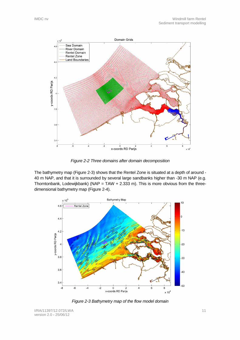
In order to obtain more detailed information in the concession zone which is called “Rentel

Zone”, a domain decomposition technique is employed to specifically refine this zone indicated

by the magenta lines in Figure 2-2. In addition, domain decomposition is applied to the river

domain but without any refinement, in order to reduce the computational time for the whole

model domain. In the Rentel domain, the grid size reaches 250 m × 250 m to 115 m × 180 m.


I/RA/11397/12.072/LWA 11 version 2.0 - 25/06/12

Figure 2-2 Three domains after domain decomposition

The bathymetry map (Figure 2-3) shows that the Rentel Zone is situated at a depth of around -

40 m NAP, and that it is surrounded by several large sandbanks higher than -30 m NAP (e.g.

Thorntonbank, Lodewijkbank) (NAP = TAW + 2.333 m). This is more obvious from the three-

dimensional bathymetry map (Figure 2-4).

Figure 2-3 Bathymetry map of the flow model domain


I/RA/11397/12.072/LWA 12 version 2.0 - 25/06/12

Figure 2-4 Three-dimensional bathymetry map of the Rentel domain

2.1.2 Boundary conditions

The SRR model is supplied by boundary conditions from the KaZNO model. In order to get a

mean tidal forcing in this domain, one year of data of tidal ranges at three stations were

statistically analysed and then a representative spring-neap tidal period was selected.

Figure 2-5 Tidal gauges in the model domain

Closed boundaries of the model domain


I/RA/11397/12.072/LWA 13 version 2.0 - 25/06/12

In fact, there are much more tidal gauges than what is shown in Figure 2-5. However, a

complete set of tidal elevations for one year can only be found at the three stations, shown as

stars in the figure.

Figure 2-6 shows the variation of tidal ranges at three observation stations during the whole

year of 2009. The tidal range at Hansweert is much higher than those at the other stations,

due to the tidal wave transformation in the estuary.

Figure 2-6 Tidal ranges at three stations in 2009

Figure 2-7 shows that the three stations have an almost identical variation pattern in terms of

the moving averaged tidal range for a spring-neap tidal cycle. The 394th spring-neap tidal

cycle marked by the black dash line in the figure was selected as the representative tidal

period to represent the mean tidal forcing of a whole year in this domain.

Table 1 shows that the tidal ranges of the selected representative tidal period at the different

three stations are all fairly close to their annual mean tidal ranges.

Table 1 Values of averaged tidal range of the selected representative tidal period and annual

mean tidal range at three stations

Location averaged tidal range of the 394th spring-neap

tidal cycle annual mean tidal

range Europlatform 164.4 cm 164.3 cm

Lichteiland Goeree 188.6 cm 188.4 cm Hansweert 441.8 cm 439.1 cm


I/RA/11397/12.072/LWA 14 version 2.0 - 25/06/12

Figure 2-7 Moving averaged tidal range for spring-neap tidal cycle at three stations

The annual representative spring-neap tidal cycle period is from 23-Jul-2009 14:00:00 to 07-

Aug-2009 01:40:00, in total 20860 minutes (14 × 24 hours 50 minutes). The figure below

shows the variation of the tidal elevation observed at the nearby tidal record station MOW0

during the representative spring-neap tidal period.

Figure 2-8 Tidal elevation observed at MOW0 station during the representative period


I/RA/11397/12.072/LWA 15 version 2.0 - 25/06/12

2.1.3 Validation

The model validation period is from 12 April 2010 to 19 April 2010. Three measuring points are

used for the model validation (Figure 2-9).

Firstly, a comparison of tidal elevation was carried out at Westhinder (Figure 2-10). There is a

good agreement between the observation and modelling result. Although the modelling result

gives a maximum overestimation of around 10% in terms of the tidal range. More calibration of

the mother model KaZNO is expected to reduce this overestimation.

The observed current velocity data at Scheur Wielingen in Figure 2-11 is actually sampled at -

7.5 m below the water surface, and is not a depth averaged velocity. Due to the scarcity of

available data, the observation point is also used to investigate the performance of the model

in a qualitative point of view. From the figure, it can be seen that the model gives a satisfactory

result compared to the observed data. The variation pattern of tidal current magnitude is

captured by the model successfully, and the direction of current velocity is reproduced by the

model quite well.

The velocity data at Lodewijkbank is collected in the Northwind (former Eldepasco) project

area near to the Rentel Zone, 0.5 m above the bottom (at -26.23 m NAP) (Figure 2-9). At this

point, the modelling result is shown to deviate from the observed data. However, the variation

characteristics of the tidal current are effectively reproduced by the model. The magnitude of

the current velocity is overestimated approximately 25% by the model, and the bias and

RMSE are 0.083 m/s and 0.16 m/s respectively. On one side, this overestimation could be

ascribed to the overestimation of the tidal range, which has been demonstrated in Figure 2-10.

On the other side, the sampling point is located at the top of the sandbank, where the

topography is highly variable (e.g. small dunes, ripples) and the hydrodynamics is locally

complex. To resolve such high variability in sea bottom would of course result in a more

detailed and refined numerical modelling scheme and associated increasing cost of

computation time. In addition, the bathymetry input in the model is different from that found in

the measurement (24.85 m vs. 26.73 m), which is also able to influence accuracy of the

modelling.


I/RA/11397/12.072/LWA 16 version 2.0 - 25/06/12

Figure 2-9 Location of observation points

Figure 2-10 Comparison of tidal elevation at Westhinder


I/RA/11397/12.072/LWA 17 version 2.0 - 25/06/12

Figure 2-11 Comparison of velocity at Scheur Wielingen


I/RA/11397/12.072/LWA 18 version 2.0 - 25/06/12

Figure 2-12 Comparison of velocity at Lodewijkbank

2.2 WAVE MODEL

2.2.1 Introduction

In order to investigate the stability of the sandy subsurface under storm conditions, a wave

model covering the sea domain of the flow model was developed using the wave module of

Delft3D (Delft3D-WAVE). This is actually the same as the stand alone wave model SWAN

(SWAN Cycle III version 40.72ABCDE) but integrated within Delft3D with a comprehensive

user interface and allows coupling with the FLOW module.

SWAN (acronym for Simulating WAves Nearshore), which is developed at the Delft University

of Technology, is a third generation spectral wave model for obtaining realistic estimates of

wave parameters in coastal areas, lakes and estuaries from given wind, bottom and current

conditions. The model is based on the wave action balance with sources and sinks.

The following wave propagation processes are represented in SWAN (only the processes

relevant to this case are given):

Refraction due to spatial variations in bottom;

Shoaling due to spatial variations in bottom;


I/RA/11397/12.072/LWA 19 version 2.0 - 25/06/12

The following wave generation and dissipation processes are represented in SWAN:

Generation by wind;

Dissipation by whitecapping;

Dissipation by bottom friction;

Wave-wave interactions (quadruplets and triads).

2.2.2 Numerical grid and bathymetry

The main wave model has a space-uniform resolution with a grid size of 1000 m × 1000 m (cf.

Figure 2-13). To obtain a higher resolution at the Rentel concession area, a wave model with a

grid size of approximately 230 m x 230 m is nested within the main wave model (cf. green grid

in Figure 2-13, this is the same grid as the FLOW detailed grid Rental Domain). In Figure 2-14,

showing the bathymetry map of the wave model, the wave monitoring station “Sandettie

Light(ship)” is indicated. The observation station is exactly situated at the western boundary of

the wave model, from which sampled wave data were used to provide the boundary conditions

for the wave model. Whereas sampled wave data from the other monitoring station

“Westhinder” were used for the validation of the wave model. Also, the wind data at

Westhinder was used to provide the wind boundary conditions of the wave model.

Figure 2-13 The wave model grids (main wave model: Wave Grid, nested wave model: Rentel

Domain) and the three domains of the flow model


I/RA/11397/12.072/LWA 20 version 2.0 - 25/06/12

Figure 2-14 Bathymetry map of the wave model and two wave monitoring stations

2.2.3 Boundary conditions

In order to determine the wave conditions for a one-year-return storm, a wave dataset of 20

years collected at Westhinder was investigated. The significant wave height was used as an

input variable to an extreme value analysis (EVA) tool developed at IMDC. Peaks of the

significant wave height were firstly picked out by the tool and shown by red diamonds in Figure

2-15.

Figure 2-15 Significant wave height observed at Westhinder from 01-July-1990 to 01-July-

2010


I/RA/11397/12.072/LWA 21 version 2.0 - 25/06/12

Based on the peaks of the significant wave height, a correlation between the significant wave

height and the return period was found by the EVA tool (Figure 2-16). The significant wave

height in a one-year return storm is about 4.353 m. The two upper panels in this figure

demonstrate the performance of the statistical model, from which a quite good agreement

between real and modelled values can be observed.

Figure 2-16 Upper panels: performance of the statistical model; lower panel: correlation

between variable level and return period.

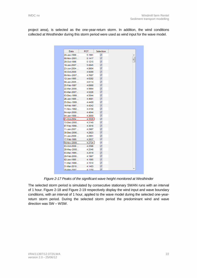
In Figure 2-17, the peaks of significant wave height are listed in a descending order. The one-

year-return storm with significant wave height of 4.353 m occurs on 21-Oct-2004. But the

sampled wave dataset at Sandettie Lightship is only available after 2005. The significant wave

height (4.299 m) of the storm occurring on 11-Jan-2007 is quite close to that (4.353 m) of one-

year-return storm. However a much larger storm with significant wave height of 5.085 m

subsequently took place on 18-Jan-2007. If the wave peak (4.299 m) would be adapted to the

lowest water at spring tide, the large storm with significant wave height of 5.085 m would be

also included in the simulation period, as a result of which the significant wave height of the

one-year-return storm becomes 5.085 m instead of 4.299 m during the simulation period.

Another storm with a similar significant wave height of 4.272 m, which occurred on 18-Nov-

2009 and was produced by a wind from west southwest (the predominant wind direction in the


I/RA/11397/12.072/LWA 22 version 2.0 - 25/06/12

project area), is selected as the one-year-return storm. In addition, the wind conditions

collected at Westhinder during this storm period were used as wind input for the wave model.

Figure 2-17 Peaks of the significant wave height monitored at Westhinder

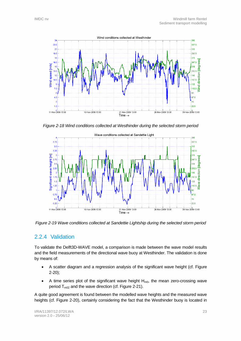
The selected storm period is simulated by consecutive stationary SWAN runs with an interval

of 1 hour. Figure 2-18 and Figure 2-19 respectively display the wind input and wave boundary

conditions, with an interval of 1 hour, applied to the wave model during the selected one-year-

return storm period. During the selected storm period the predominant wind and wave

direction was SW – WSW.


I/RA/11397/12.072/LWA 23 version 2.0 - 25/06/12

Figure 2-18 Wind conditions collected at Westhinder during the selected storm period

Figure 2-19 Wave conditions collected at Sandettie Lightship during the selected storm period

2.2.4 Validation

To validate the Delft3D-WAVE model, a comparison is made between the wave model results

and the field measurements of the directional wave buoy at Westhinder. The validation is done

by means of:

A scatter diagram and a regression analysis of the significant wave height (cf. Figure

2-20);

A time series plot of the significant wave height Hm0, the mean zero-crossing wave

period Tm02 and the wave direction (cf. Figure 2-21).

A quite good agreement is found between the modelled wave heights and the measured wave

heights (cf. Figure 2-20), certainly considering the fact that the Westhinder buoy is located in


I/RA/11397/12.072/LWA 24 version 2.0 - 25/06/12

the main wave model with a coarse grid (1000 m x 1000 m). The spread of points around the

regression line (red line in graph) is mainly due to the stationary mode of the simulations. In

other words, the time it takes for a wave to travel from e.g. the Sandettie Lightship point to the

Westhinder point and also variations in wind speed, direction and water level between time

steps is not taken into account by the stationary simulations.

This good agreement is more apparent when comparing the time series (cf. Figure 2-21). The

mean zero-crossing wave period Tm02 and the wave direction time series also show quite good

agreement. Due to a difference in calculation of the wave period Tm02 in SWAN and in the

buoy measurements (IMDC, 2009), a correction was applied to the Tm02 values calculated by

SWAN to account for this difference. This has no effect on the wave periods within the model.

Due to this good agreement between simulation and measurement, no further calibration was

deemed necessary.

Figure 2-20 One-on-one relation between the significant wave height calculated by Delft3D-

WAVE and measured at the Westhinder buoy location


I/RA/11397/12.072/LWA 25 version 2.0 - 25/06/12

Figure 2-21 Validation of the Delft3D-WAVE model with field measurements of the directional wave buoy at the Westhinder bank. Comparison of the

time series of the significant wave height Hm0, the mean zero-crossing wave period Tm02 and wave direction


I/RA/11397/12.072/LWA 26 version 2.0 - 25/06/12

2.3 SEDIMENT TRANSPORT MODEL

For the sediment transport, the Van Rijn TRANSPOR2000 approach is employed in the model

(Van Rijn, 2003). The bed load transport and suspended transport are distinguished based on

the reference height, below which the movement of sediment is treated as bed load transport

whereas above the movement of sediment is treated as suspended transport. More detailed

information about the approach can be found in the Delft3D-FLOW User Manual.

2.3.1 Boundary conditions and median grain size

In this model, the boundary condition for the sediment is specified by “equilibrium”

concentrations. The equilibrium concentration is a function of the local current velocity. By this

specification, the sediment concentrations are equal to those just inside the model domain,

near-perfectly adapted sediment flux flows into the domain with little sedimentation or erosion

near the model boundaries (Delft3D-FLOW User Manual). In addition, the morphology is not

updated in the modelling of the sediment transport.

According to the grain size distribution map (Figure 2-22), the sediments in the Rentel Zone

mainly consist of sand between 300 to 350 µm. Some small areas contain sand from 250-

300 µm and from 350-400 µm. With the model updating of the grain size distribution is not

feasible. Therefore a uniform grain size has to be selected. The model has been run

respectively with grain sizes of 250, 350 and 400 µm for the selected representative spring-

neap tidal cycle. The three scenarios with different grain sizes demonstrate almost the same

direction of residual sediment transport (results are not shown here). 250 µm logically shows

the highest residual sediment transport, maximally twice as much as 400 µm, while 350 µm

only displays slightly larger residual sediment transport than 400 µm. Due to the domination of

sand between 300 to 350 µm in the Rentel Zone, a space-uniform grain size of 350 µm is

adopted in the model.


I/RA/11397/12.072/LWA 27 version 2.0 - 25/06/12

Figure 2-22 Map of the grainsize distribution (adapted after Verfaillie et al., 2006). The Rentel

concession zone is the brown hatched area in the centre of the figure, the dark blue contour is

the detailed numerical model domain.


I/RA/11397/12.072/LWA 28 version 2.0 - 25/06/12

3. RESULTS

3.1 SUMMER CONDITION (TIDAL CURRENTS ONLY)

In this study, the morphological evolution and the sediment transport in the Rentel Zone are

investigated during two conditions. In summer conditions, only tidal forcing is considered for

the formerly selected representative spring-neap tidal period. While in winter conditions, the

tidal and wave forcings are coupled together in model.

Figure 3-1 shows that the Rentel Zone is situated between two large banks, indicated by the -

25 m isobath contour lines (the northern one is Lodewijkbank; the southern one is

Thorntonbank). The red cross and triangle indicate the location of points for inspection of time

series modelling results.

Figure 3-1 Bathymetry map with isobath contour lines of -25 m NAP; red cross and triangle

label two points in the Rentel Zone for inspection of time series variables

3.1.1 Currents

The tidal current velocity and elevation at two points in the Rentel Zone (cf. Figure 3-1) is

presented in Figure 3-2 and Figure 3-3. The time series modelling results are displayed for the

selected representative spring-neap tidal period. The currents are completely driven by tidal

forcing without any meteorological forcing.

The red triangle point is located at a slightly shallower area near to Thorntonbank, showing a

little larger flood current, while the cross point in the deeper area exhibits stronger ebb

currents. This is probably due to convergence of the flow to the deeper part during the ebb


I/RA/11397/12.072/LWA 29 version 2.0 - 25/06/12

phase. The difference of current velocity between these two points is, however, quite small,

maximally not more than 10%. The current velocity at these two points roughly ranges

between 0.08 and 0.95 m/s.

Figure 3-2 Time series showing current velocity magnitude and tidal elevation at the red cross

point

Figure 3-3 Time series showing current velocity magnitude and tidal elevation at the red

triangle point

Figure 3-4 displays the tidal current ellipses in the area in and around the Rentel Zone.

Currents in the Rentel Zone show a large eccentricity with smaller velocity at the minor axis

during the flow reversal, while those at the top of the banks are more rotary with larger

velocities at the minor axis during the flow reversal, in particular at the Thorntonbank.


I/RA/11397/12.072/LWA 30 version 2.0 - 25/06/12

Figure 3-4 Map of averaged current ellipses in summer conditions with bathymetry as

background; the averaged current ellipses are calculated over the representative spring-neap

tidal cycle; the grid resolution of one ellipse is about 1000m × 500m.

Figure 3-5 Map of averaged current velocity magnitude calculated over the representative

spring-neap tidal cycle in summer conditions with isobath lines of -25 m NAP


I/RA/11397/12.072/LWA 31 version 2.0 - 25/06/12

Figure 3-5 and Figure 3-6 give respectively the averaged and maximal velocity magnitude

over the representative spring-neap tidal cycle. Strong currents occur at the top of the banks,

the hydrodynamic forcing in the Rentel Zone is relatively low. The northern part of the Rentel

Zone (up to the flank of the Lodewijkbank) seems to be more energetic than the southern part.

The averaged velocity magnitude in the Rentel Zone ranges between 0.47 and 0.54 m/s, and

the maximal velocity can reach 0.98 m/s at the northern boundary of the Rentel Zone.

Figure 3-6 Map of maximal current velocity magnitude over the representative spring-neap

tidal cycle in summer conditions with isobath lines of -25 m NAP

The residual currents presented in Figure 3-7 and Figure 3-17 take the local water depth into

account at each point. The calculation of the residual current follows the formulation as

below:

where and hi are current velocity and water depth for a certain location at the time point i,

and h is the local real water depth without the effect of tidal elevation change.

Figure 3-7 shows that residual currents flow from southwest to northeast (without any effect of

meteorological forcing). The residual currents are apparently lower in the Rentel Zone

compared to those at the banks. The highest residual current reaches around 0.14 m/s and

occurs at the top of the Thorntonbank. In the Rentel Zone, the residual current is around

0.07 m/s, and the maximal one reaches around 0.11 m/s at the northern boundary - at the

rising flank of the Lodewijkbank.


I/RA/11397/12.072/LWA 32 version 2.0 - 25/06/12

Figure 3-7 Map of the residual current calculated over the representative spring-neap tidal

cycle in summer conditions with residual velocity magnitude as background and isobath lines

of -25 m NAP

3.1.2 Bottom shear stress

In summer conditions, under tidal forcing only, the distribution of the bottom shear stress

coincides with that of the velocity magnitude. Figure 3-8 and Figure 3-9 respectively show the

averaged and maximal bottom shear stress over the representative spring-neap tidal cycle. In

the Rentel Zone the averaged bottom shear stress ranges between 0.5 and 0.8 Pa, and the

maximal one reaches around 2.2 Pa.


I/RA/11397/12.072/LWA 33 version 2.0 - 25/06/12

Figure 3-8 Map of the averaged shear stress magnitude calculated over the representative

spring-neap tidal cycle in summer condition with isobath lines of -25m

Figure 3-9 Map of maximal shear stress magnitude over the representative spring-neap tidal

cycle in summer condition with isobath lines of -25m


I/RA/11397/12.072/LWA 34 version 2.0 - 25/06/12

3.1.3 Sediment transport and morphological evolution

Figure 3-10 Map of residual sediment transport calculated over the representative spring-neap

tidal cycle in summer conditions with transport rate as background and isobath lines of -25 m

In the sediment transport model, the morphology update was not taken into account.

Therefore sedimentation and erosion are not able to cause any change on the initial

bathymetry. Figure 3-10 shows that the residual sediment transport is generally consistent with

the residual current presented in Figure 3-7. Most of the residual sediment transport is directed

to the northeast. The largest transport rate takes place at the top of Thorntonbank, but its

transport direction is different from the residual current direction at the same location. In the

Rentel zone the residual sediment transport is quite low, and the highest one is not larger than

4.10-5

m3/s/m. From Figure 3-11, it can be also seen that the Rentel Zone is relatively stable

with lower sedimentation and erosion, where the change of sediment thickness on the bed

after a spring-neap cycle is limited to around 0.02 m.


I/RA/11397/12.072/LWA 35 version 2.0 - 25/06/12

Figure 3-11 Map of sedimentation and erosion calculated over the representative spring-neap

tidal cycle in summer conditions with vectors of residual sediment transport and isobath lines

of -25 m NAP

The modelling results demonstrate a very good correlation between the current velocity

magnitude and the sediment transport rate in summer conditions only driven by tides (Figure

3-12). The largest transport reaches over 4.10-5

m3/s/m during spring tide, whereas during

neap tide the transport rate is reduced by a factor of more than 10, and is not more than

3.10-6

m3/s/m. The resulting sediment transport volume (without porosity) over the spring-neap

tidal cycle (23-Jul 14:00 ~ 07-Aug 01:40) is 5.67 m3/m at the observation point. Over the full

spring tide (red line in Figure 3-12, 23-Jul 19:00 ~ 24-Jul 19:50) it is 1.00 m3/m and over the

neap tide (magenta line in Figure 3-12, 01-Aug 01:20 ~ 02-Aug 02:10) it is 0.028 m3/m.

Figure 3-12 Time series of modelled sediment transport and velocity magnitude during the

representative spring-neap tidal cycle in summer conditions at the red triangle point


I/RA/11397/12.072/LWA 36 version 2.0 - 25/06/12

3.2 WINTER CONDITION (TIDES + WAVES)

For the winter conditions, a one-year-return storm is simulated by the wave model, which is

coupled with the flow model to simulate the sediment transport during the representative

spring-neap tidal cycle.

3.2.1 Currents and waves

In order to consider the worst case scenario, the wave peak of the one-year-return storm is

shifted to the lowest water at spring tide (cf. red arrow in Figure 3-13).

Figure 3-13 Time series of modelled significant wave height and tidal elevation during the

representative spring-neap tidal cycle in winter conditions at the red triangle point

Compared to the summer conditions, current velocities in winter conditions do not exhibit a

pronounced difference (Figure 3-14, Figure 3-15, Figure 3-16 and Figure 3-17). Currents in the

Rentel Zone are less rotary with smaller velocities at the minor axis during the flow reversal

(Figure 3-14). The averaged velocity magnitude in the Rentel Zone ranges between 0.47 and

0.54 m/s, and the maximal one is lower than 1 m/s (Figure 3-15 and Figure 3-16). The residual

current is quite low in the Rentel Zone, and the maximal is around 0.11 m/s at the northern

boundary.

Figure 3-18 and Figure 3-19 present the significant wave height calculated by the wave model.

In the Rentel Zone, the resolution of the computational grids in the wave model is around 120-

190 m × 200-210m, in which the two large banks Lodewijkbank and Thortonbank are explicitly

described. It can be clearly seen from the figures that the wave from the southwest is

drastically dissipated when it travels over the banks, in particular the Thortonbank. The

averaged significant wave height in the Rentel Zone is around 2 m during the storm period,

and the maximal one reaches about 4.5 m.


I/RA/11397/12.072/LWA 37 version 2.0 - 25/06/12

Figure 3-14 Map of averaged current ellipses in winter conditions with bathymetry as

background; the averaged current ellipses are calculated over the representative spring-neap

tidal cycle; the grid resolution of one ellipse is about 1000 m × 500 m

Figure 3-15 Map of averaged current velocity magnitude calculated over the representative

spring-neap tidal cycle in winter conditions with isobath lines of -25 m NAP


I/RA/11397/12.072/LWA 38 version 2.0 - 25/06/12

Figure 3-16 Map of maximal current velocity magnitude over the representative spring-neap

tidal cycle in winter conditions with isobath lines of -25 m NAP

Figure 3-17 Map of residual current calculated over the representative spring-neap tidal cycle

in winter conditions with residual velocity magnitude as background and isobath lines of -25 m

NAP


I/RA/11397/12.072/LWA 39 version 2.0 - 25/06/12

Figure 3-18 Map of averaged significant wave height calculated over the representative spring-

neap tidal cycle in winter conditions with isobath lines of -25 m NAP

Figure 3-19 Map of maximal significant wave height over the representative spring-neap tidal

cycle in winter conditions with isobath lines of -25 m NAP


I/RA/11397/12.072/LWA 40 version 2.0 - 25/06/12

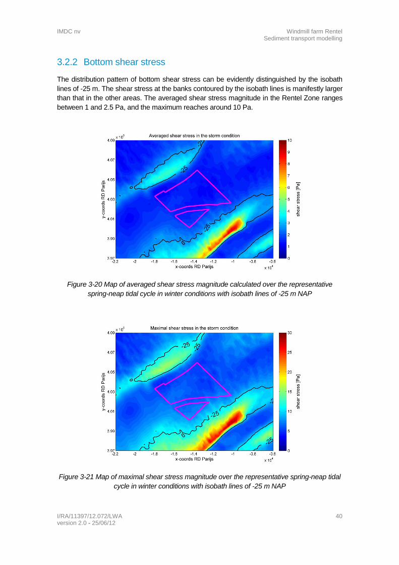
3.2.2 Bottom shear stress

The distribution pattern of bottom shear stress can be evidently distinguished by the isobath

lines of -25 m. The shear stress at the banks contoured by the isobath lines is manifestly larger

than that in the other areas. The averaged shear stress magnitude in the Rentel Zone ranges

between 1 and 2.5 Pa, and the maximum reaches around 10 Pa.

Figure 3-20 Map of averaged shear stress magnitude calculated over the representative

spring-neap tidal cycle in winter conditions with isobath lines of -25 m NAP

Figure 3-21 Map of maximal shear stress magnitude over the representative spring-neap tidal

cycle in winter conditions with isobath lines of -25 m NAP


I/RA/11397/12.072/LWA 41 version 2.0 - 25/06/12

3.2.3 Sediment transport and morphological evolution

The pattern of residual sediment transport has not changed in winter conditions compared to

that in summer conditions (Figure 3-22). The transport rate at the top of the banks seems to be

more visibly enhanced than in other locations. The largest residual sediment transport in the

Rentel Zone is about 5.10-5

m3/s/m.

The pattern of sedimentation and erosion in winter conditions is also quite consistent with that

in summer conditions (Figure 3-23). Corresponding to the enhancement of the transport rate at

the top of the banks, more visible changes of sediment thickness can be observed at these

locations. In the Rentel Zone, the seabed still looks quite stable with little sedimentation and

erosion. Because of the resolution of the model, individual sand dunes cannot be discerned.

Nevertheless, some lateral alternating bands can be observed in Figure 3-23, which might

represent vertical erosion and sedimentation on adjacent crests and troughs of sand dunes.

The morphological changes are in the order of 2 cm after a spring-neap-tidal cycle of 15 days

with storm conditions. However, these results should not be extrapolated to long term

estimations on dune migration, as detailed dune migration processes and morphology

updating are not taken into account in the model.

Figure 3-22 Map of residual sediment transport calculated over the representative spring-neap

tidal cycle in winter conditions with transport rate as background and isobath lines of -25 m

NAP


I/RA/11397/12.072/LWA 42 version 2.0 - 25/06/12

Figure 3-23 Map of sedimentation and erosion calculated over the representative spring-neap

tidal cycle in winter conditions with vectors of residual sediment transport and isobath lines of -

25 m NAP


I/RA/11397/12.072/LWA 43 version 2.0 - 25/06/12

4. DISCUSSION

The difference of sediment transport between the summer and winter conditions at the two

fixed locations (cf. red triangle and cross shown in Figure 3-1) is respectively presented in

Figure 4-1 and Figure 4-2. These two figures show a very similar variation of sediment

transport in case of only tides and in case of a combination of tide and waves. From these

figures, can be concluded that in winter conditions the sediment transport is not only

dependent on the significant wave height, but that the tidal current plays an important role on

it. In fact the significant wave height is continuously large for about 4 days after 30 July, but

during this period the sediment transport is not raised to a very high level by these conditions.

Compared to the transport level in summer conditions, the transport rate is doubled under the

effects of waves, but the absolute level is still quite low due to the weak tidal current at neap

tide.

While during the period between 23 July and 30 July, the sediment transport is able to reach a

very high level when the large wave occurs concurrently with the strong current at spring tide.

In this case, the sediment transport is also doubled compared to that affected by tides only.

Figure 4-1 Time series of modelled sediment transport in summer and winter conditions, and

modelled significant wave height in winter conditions at the red triangle point


I/RA/11397/12.072/LWA 44 version 2.0 - 25/06/12

Figure 4-2 Time series of modelled sediment transport in summer and winter conditions, and

modelled significant wave height in winter conditions at the red cross point

At both of the two points, sedimentation takes place (Figure 4-3 and Figure 4-4). At spring tide

the sedimentation increases quite fast, while at neap tide the increase becomes very slow.

During the whole spring-neap tidal period, the sedimentation is about 0.0063 m at the triangle

point and 0.0046 m at the cross point in summer conditions with the effect of only tides, while

in winter conditions the sedimentation is increased by about 67% and 56% at the triangular

and cross points respectively under the effects of tides and waves.

Figure 4-3 Time series of modelled change of sediment thickness in summer and winter

conditions at the red triangle point


I/RA/11397/12.072/LWA 45 version 2.0 - 25/06/12

Figure 4-4 Time series of modelled change of sediment thickness in summer and winter

conditions at the red cross point


I/RA/11397/12.072/LWA 46 version 2.0 - 25/06/12

5. CONCLUSIONS

In this study, the hydrodynamic model Delft3D-FLOW and standalone wave model Delft3D-

WAVE were firstly validated against the measured data in the neighbourhood of the study

area. The tidal current at Lodewijkbank seems to be overestimated approximately 25% by the

model. This could be attributed to the overestimation of the tidal range due to the boundary

conditions generated by the mother model, and to the insufficient resolution of the

computational grids to resolve the highly complex topography at the sandbanks. However,

variation characteristics of tidal current and elevation were reproduced quite well by the model,

and the agreement between the modelling results and measured data is satisfactory. The

wave characteristics under storm conditions (with one-year-return period) were also

successfully reproduced by the wave model in view of the comparison of significant weight

height, wave period and wave direction between the modelling results and measured data.

The sediment transport in the Rentel Zone is calculated separately for summer conditions and

winter conditions. In summer conditions, the sediment transport is only affected by tidal

currents. The residual current flows from the southwest to northeast. In the Rentel Zone, the

currents are less rotary than those at its surrounding banks. The averaged velocity magnitude

in the Rentel Zone ranges between 0.47 and 0.54 m/s, the maximum is 0.98 m/s at the

northern boundary of the Rentel Zone, up to the flank of the Lodewijkbank. The residual

sediment transport is quite low in the Rentel Zone, and the maximum is not larger than 4.10-5

m3/s/m. The map of sedimentation and erosion shows that the seabed in the Rentel Zone is

quite stable, and the change of sediment thickness is limited to a level of around 0.02 m during

the representative spring-neap tidal period.

In winter conditions, the sediment transport is affected by combination of tidal currents and

waves. To consider the worst case, a peak of waves is intentionally shifted to the lowest water

at spring tide. The patterns of current velocity do not seem to be significantly affected by the

wave coupling. However, the bottom shear stress is evidently enhanced from 0.5-0.8 Pa in

summer conditions to 1.0-2.5 Pa in winter conditions, and the maximum is locally around 10

Pa in the Rentel Zone. The sediment transport is not only dependent on the significant wave

height, the tidal current also plays an important role on it. The largest transport takes place at

the moment when the currents and waves are both large. The largest residual sediment

transport in the Rentel Zone is about 5.10-5

m3/s/m over the representative spring-neap tidal

cycle, and the erosion and sedimentation is also quite small, in the order of 2 cm over the

vertical. The seabed in the Rentel Zone seems to be rather stable over the modelled period in

case of storm conditions with one-year-return period. Dune migration rates on the long term

cannot be deduced from these results, although it is expected that dune mobility is lower in the

swales between sandbanks, than on top of the sandbanks.


I/RA/11397/12.072/LWA 47 version 2.0 - 25/06/12

6. REFERENCES

Ashley, G.M. (1990). Classification of large-scale subaqueous bedforms: a new look at an old

problem. Journal of Sedimentary Petrology, 60(1): 160-172.

IMDC (2009). Afstemming Vlaamse en Nederlandse voorspelling golfklimaat op ondiep water.

Deel 4: Technisch wetenschappelijke bijstand: Traject Onderzoek. I/RA/11273/09.007/SDO. In

opdracht van het Waterbouwkundig Laboratorium.

Van Rijn, L.C.(2003). Sand transport by currents and waves; general approximation formulae.

Unpublished paper describing TRANSPOR2000 model.

Verfaillie, E., Van Lancker, V. and Van Meirvenne, M. (2006). Multivariate geostatistics for the

predictive modelling of the surficial sand distribution in shelf seas. Continental Shelf Research

26, 2454-2468.

Environmental Impact Report windmill farm Rentel transport...Rentel NV Environmental Impact Report...

Documents

Transcript of Environmental Impact Report windmill farm Rentel transport...Rentel NV Environmental Impact Report...