Environment Characterization for Non-Recontaminating ... · Environment Characterization for...

Environment Characterization forNon-Recontaminating Frontier-Based

Robotic Exploration

Mikhail Volkov, Alejandro Cornejo, Nancy Lynch, and Daniela Rus

Computer Science and Artificial Intelligence LaboratoryMassachusetts Institute of Technology, Cambridge, MA 02139{mikhail,acornejo,lynch,rus}@csail.mit.edu

Abstract. This paper addresses the problem of obtaining a concise descriptionof a physical environment for robotic exploration. We aim to determine the num-ber of robots required to clear an environment using non-recontaminating ex-ploration. We introduce the medial axis as a configuration space and derive amathematical representation of a continuous environment that captures its under-lying topology and geometry. We show that this representation provides a concisedescription of arbitrary environments, and that reasoning about points in this rep-resentation is equivalent to reasoning about robots in physical space. We leveragethis to derive a lower bound on the number of required pursuers. We provide atransformation from this continuous representation into a symbolic representa-tion. Finally, we present a generalized pursuit-evasion algorithm. Given an envi-ronment we can compute how many pursuers we need, and generate an optimalpursuit strategy that will guarantee the evaders are detected with the minimumnumber of pursuers.

Keywords: swarm robotics, frontier-based exploration, distributed pursuit-evasion, environment characterization, mathematical morphology, planargeometry, graph combinatorics, game determinacy

1 IntroductionThis paper deals with the problem of developing a concise representation of a physicalenvironment for robotic exploration. We address a specific type of exploration scenariocalled pursuit-evasion. In this scenario, a group of robots are required to sweep an un-explored environment and detect any intruders that are present. Pursuit-evasion is anexample of non-recontaminating exploration, whereby an initially unexplored and con-taminated region is cleared while ensuring that the cleared region does not becomecontaminated again. Pursuit-evasion is a useful model for many applications such assurveillance, security and military operations. Aside from the classical pursuit-evasionproblem, there are other scenarios that motivate non-recontaminating exploration. Oneexample is cleaning up an oil spill in the ocean using robots, where the oil can leakinto previously decontaminated water whenever part of the frontier is not guarded bya robot. Another example is a disaster response scenario such as after an earthquake,where a group of robots is required to locate all survivors in some inaccessible area,while the survivors are possibly moving in the environment.

2 Environment Characterization for Non-Recontaminating Robotic Exploration

1.1 Related Work

Visibility-based pursuit-evasion in continuous two-dimensional space was first intro-duced in [25]. Frontier-based exploration was introduced in [28] and extended to mul-tiple robots in [29]. In [7] the authors consider limited visibility frontier-based pursuit-evasion in non-polygonal environments, making use of the fact that not allowing recon-tamination means we do not need to store a map of the environment; here a distributedalgorithm is presented which works by locally updating the frontier formed by the sen-sor footprints of the robots. Another distributed model was more recently considered in[3]. Limited visibility was also considered in [23] which presents an algorithm for clear-ing an unknown environment without localization. In [8] the problem was consideredfor a single searcher in a known environment. Generally speaking, these algorithmsdo the correct thing locally, but do not rely on, or make any guarantees for, a globaldescription of an environment. As such, they may not be guaranteed to terminate.

Environment characterization for pursuit-evasion has been considered for polygo-nal spaces. In [11], [12] pursuit-evasion in connected polygonal spaces is investigated,and tight bounds derived on the number of pursuers necessary based on the number ofpolygon edges and holes. In [19] basic environment characterization is established, bymeans of a general decomposition concept based on a finite complex of conservativecells. In [27] similar ideas were explored, and several metrics proposed for primitivecharacterization of polygonal spaces. We highlight that these studies considered robotsequipped with infinite range visibility sensors deployed in polygonal spaces. Conse-quently the scope of environment characterization was limited. By contrast we considerlimited visibility sensors, and we do not require the environment to be polygonal.

The medial axis has previously been studied in the context of robotic navigation.For example, in [10], [13], [26] the medial axis was used as a heuristic for probabilisticroadmap planning. One of the key features that makes the medial axis attractive for suchapplications is that it captures the connectivity of the free space. In this work, we usethe medial axis to similarly capture the underlying topological and geometric propertiesof our environment, and use it to transform the problem into a graph formulation.

Pursuit-evasion on graphs that are representations of some environment goes backas early as [20], [21]. Randomized pursuit strategies on a graph are considered in [1].Roadmap-based pursuit-evasion is considered in [14] and [22] where the pursuer andevader share a map and act according to different rules. In [22] a graph-based represen-tation of the environment is used to derive heuristic policies in various scenarios. Morerecently, [17] presents a graph-based approach to the pursuit-evasion problem wherebyagents use blocking or sweeping actions to detect all intruders in the environment. In[15] and [16] the more general graph variant of the problem was reduced to a tree byblocking edges. Although discrete graph-based models offer termination and correct-ness guarantees, they assume the world is suitably characterized and make no referenceto the underlying physical geometry of the environment that is being represented.

The aim of this paper is to bridge the different levels of abstraction that work todate has been grounded in. We make use of the medial axis as a configuration space toderive a robust representation of a continuous environment that captures its underlyingproperties. We use the medial axis leveraged by existing exploration models to build aconcise representation of arbitrary environments in continuous two-dimensional space.

Environment Characterization for Non-Recontaminating Robotic Exploration 3

We then transform this representation into the discrete domain. First, this allows usto calculate bounds on the number of pursuers required to clear an environment, andto provide termination guarantees for existing pursuit-evasion algorithms. Second, thisestablishes an application platform for existing graph-based algorithms making themapplicable to continuous environment descriptions.

1.2 Paper Organization

This paper is organized as follows. In Section 2 we provide a formal model for non-recontaminating exploration and state the problem that we are addressing. In Section3 we introduce the medial axis as a configuration space and show that reasoning aboutpoints in this space is equivalent to reasoning about robots in the physical world. Weformalize the notion of width, corridors and junctions and derive bounds on the numberof robots required to traverse a junction. In Section 4 we present a transformation fromthis continuous configuration space into a symbolic representation in the discrete do-main. Finally, we present an optimal pursuit-evasion algorithm, and prove correctnessfor this algorithm.

2 Problem FormulationWe now present a formal model of the problem we are addressing. Our model buildson the notation and terminology introduced in [7]. We have a team of n explorationrobots deployed in the Euclidean plane R2. Each robot is equipped with a holonomic(uniform in all orientations) sensor that records a line of sight perception of the envi-ronment within a maximum sensing radius r. We assume that two robots can reliablycommunicate if they are within line of sight of each other and if the distance betweentheir positions is less than or equal to 2r.

The position of a robot is constrained to be within some free region Q, which is aclosed compact subset of R2. The obstacle region B makes up the rest of the world,and is defined as the complement of Q. In this paper we require both Q and B tobe connected spaces, which means there are no holes in the environment. We definethe obstacle boundary ∂B as the oriented boundary of the obstacle region (which bydefinition is the oriented boundary of the free region).

We assume a continuous time model, i.e. time t ∈ R≥0. Let Hit be the holonomic

sensor footprint of robot i at time t, which is defined as the subset of Q that is withindirect line of sight of robot i and within distance r of robot i. Formally, if p ∈ R2 is theposition of robot i at time t, then Hi

t = {x ∈ Q | d(p, x) ≤ r ∧ ∀y ∈[px], y ∈ Q}

where d(x, y) is the Euclidean distance between x and y (see Fig. 1a). Let Ht be theunion of the sensor footprints of all robots at some time t, given byHt =

⋃ni=0H

it . This

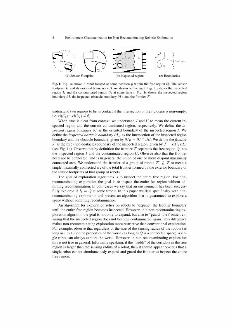
corresponds to the region being sensed by the robots at time t. We define the inspectedregion It ⊆ Q as the union at time t of all previously recorded sensor footprints, givenby It = {p ∈ R2 | ∃t0 ∈ [0, t] such that p ∈ Ht0}. The contaminated region (orunexplored region) Ut is defined as the free space that has not been inspected by timet, given by Ut = Q \ It (see Fig. 1b). Note that at time t = 0 the contaminated regionis given by Q \H0. We define the cleared region Ct ⊆ It as the inspected region that isnot currently being sensed, given by Ct = It \Ht. We say that recontamination occursat time t if the cleared region Ct comes in contact with the contaminated region Ut (we


(a) Sensor Footprint (b) Inspected region (c) Boundaries

Fig. 1: Fig. 1a shows a robot located at some position p within the free region Q. The sensorfootprint H and its oriented boundary ∂H are shown on the right. Fig. 1b shows the inspectedregion It and the contaminated region Ut at some time t. Fig. 1c shows the inspected regionboundary ∂I , the inspected obstacle boundary ∂IB and the frontier F .

understand two regions to be in contact if the intersection of their closure is non-empty,i.e. cl(Ct) ∩ cl(Ut) 6= ∅).

When time is clear from context, we understand I and U to mean the current in-spected region and the current contaminated region, respectively. We define the in-spected region boundary ∂I as the oriented boundary of the inspected region I . Wedefine the inspected obstacle boundary ∂IB as the intersection of the inspected regionboundary and the obstacle boundary, given by ∂IB = ∂I ∩ ∂B. We define the frontierF as the free (non-obstacle) boundary of the inspected region, given by F = ∂I \ ∂IB(see Fig. 1c). Observe that by definition the frontier F separates the free region Q intothe inspected region I and the contaminated region U . Observe also that the frontierneed not be connected, and is in general the union of one or more disjoint maximallyconnected arcs. We understand the frontier of a group of robots F ′ ⊆ F to mean asingle maximally connected arc of the total frontier formed by the exterior boundary ofthe sensor footprints of that group of robots.

The goal of exploration algorithms is to inspect the entire free region. For non-recontaminating exploration the goal is to inspect the entire fee region without ad-mitting recontamination. In both cases we say that an environment has been success-fully explored if It = Q at some time t. In this paper we deal specifically with non-recontaminating exploration and present an algorithm that is guaranteed to explore aspace without admitting recontamination.

An algorithm for exploration relies on robots to “expand” the frontier boundaryuntil the entire free region becomes inspected. However, in a non-recontaminating ex-ploration algorithm the goal is not only to expand, but also to “guard” the frontier, en-suring that the inspected region does not become contaminated again. This differencemakes non-recontaminating exploration more restrictive than conventional exploration.For example, observe that regardless of the size of the sensing radius of the robots (aslong as r > 0), or the properties of the world (as long as Q is a connected space), a sin-gle robot can always explore the world. However, in non-recontaminating explorationthis is not true in general. Informally speaking, if the “width” of the corridors in the freeregion is larger than the sensing radius of a robot, then it should appear obvious that asingle robot cannot simultaneously expand and guard the frontier to inspect the entirefree region.


Consider the simple rectangular free region Q shown in Fig. 1b. We can reason thatif the width of Q is less than the sum of the sensor diameters of the n robots, then theenvironment can be explored without admitting recontamination. However, even in thissimple example it is not completely clear what is meant by width. Notice that if weconsider width to be the distance from the left to the right border then this reasoningfails — in this case width would specifically mean the smaller of the two dimensions.So it is already non-trivial how to characterize a very simple environment, and thingsbecome much more complicated in non-rectangular environments.

In this paper we study the relationship between an environmentQ, the sensor radiusr, and the number of robots n required for non-recontaminating exploration of Q. Intu-ition tells us that corridor width and junctions are important features. We formalize thenotion of corridors and junctions and present a general method for computing a con-figuration space representation of the environment that captures this intuition. We showthat this representation provides a concise description of arbitrary environments.

A canonical example of non-recontaminating exploration is pursuit-evasion. In thisscenario there is a group of robot pursuers and a group of robot evaders deployed inthe free region Q. The evaders are assumed to be arbitrarily small and fast. The goalof the pursuers is to catch the evaders (by detecting their presence within the sensorfootprint), and the goal of the evaders is to avoid getting caught. Whenever part of thefrontier is not being guarded by the pursuers, the evaders can move undetected from thecontaminated region to the previously inspected region, thereby recontaminating it.

3 Environment AnalysisIn this section we present the medial axis as a configuration space and show that rea-soning about points in this configuration space is equivalent to reasoning about robotsin physical space. First, we establish the necessary geometric framework, accompaniedby a series of definitions and claims. Second, we introduce an exploration model in thisconfiguration space and justify that it allows us to reason about the physical movementof the robots in the environment.

3.1 Environment Geometry

The distance transform is a mapping D : R2 → R where D(x) = miny∈B {d(x, y)}and d(x, y) is the Euclidean distance between x and y (extending definition in [5] to thecontinuous domain) (see Fig. 2b). Observe that by definition if x /∈ Q then D(x) = 0.The distance transform of a point x ∈ Q captures the notion of “undirected width” of aregion around a point x in free space, that is we get a measure of how wide or narrow aregion is without being explicit about orientation.

The medial axis or skeleton S of a free space is defined as the locus of the centersof all maximal inscribed circles in the free space [4] (see Fig. 2c). Equivalently, theskeleton can be defined as the locus of quench points of a fire that has been set toa grass meadow at all points along its boundary [2], [24]. The skeleton captures thetopology of the free space, and aids us in determining which parts of an environmentshould be considered “corridors” and which parts should be considered “junctions” ofmultiple corridors.

The degree of a point x ∈ S is given by the function θ : S → N>0 which mapsevery point on the skeleton to a natural number k. Specifically, we define a point x ∈ S


(a) Environment image (b) Distance transform (c) Skeleton (d) Relief map

Fig. 2: The environment is represented by a binary image in Fig. 2a. Fig. 2b shows the distancetransform D of the environment. Fig. 2c shows the skeleton S. Fig. 2d shows the relief mapquantization. The relief contours indicate multiples of the sensing radius r.

to have degree θ(x) = k if there exists an a ∈ R>0 such that ∀ε ∈ (0, a] a circlecentered at x of radius ε intersects the skeleton S at exactly k points.

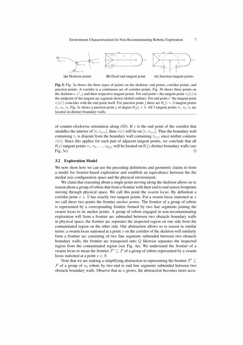
Borrowing notation from [6], we use the degree of a point x ∈ S to distinguishbetween three types of points on the skeleton: corridor points, end points and junctionpoints. Specifically, for a point x ∈ S, we say x is an end point if θ(x) = 1, x is acorridor point if θ(x) = 2, and x is a junction point if θ(x) > 2 (see Fig. 3a). We referto a continuous arc of corridor points on the skeleton simply as a corridor.

An alternative definition for θ(·) can be stated as follows. For a point x ∈ S let Cbe the maximal inscribed circle centered at x, and let G be the intersection of this circlewith the obstacle boundary, given by G = C ∩ ∂B. (Observe that by definition C hasradiusD(x) 6= 0, and since C is maximal, G is non-empty.) Then θ(x) is defined as thenumber of maximally connected arcs in G. This definition for for θ(·) is equivalent tothe previous one [4], [9], [18].

Let G1, G2, . . . , Gθ(x) be the set of maximally connected arcs of G. Note that inmost cases these arcs are in fact just single points, which corresponds to the intuitivenotion of the circle being tangent to the boundary at these points. A cursory glancereveals that this is the case for most corridor points and junction points. For end pointsthat lie on the obstacle boundary, the tangent point coincides with the end point itself.However, the generality is necessary in a few special cases, such as end points of regionsthat taper off in a sector. In these cases the maximal inscribed circle C will be tangentto the obstacle boundary at a continuous arc segment of points. In order to simplify thediscussion we define the tangent points τ1(x), τ2(x), . . . , τθ(x)(x) of a point x ∈ S asthe midpoints of the tangent arcs G1, G2, . . . , Gθ(x) (see Fig. 3b).

We define a boundary wall as a maximally connected arc segment of the obstacleboundary ∂B that does not contain a tangent point of any end point. Formally ∂B0 ⊂∂B is a boundary wall if it is a maximally connected arc segment such that ∀e ∈ S |θ(e) = 1, τ(e) /∈ ∂B0.

Lemma 1. For a junction point j ∈ S, the θ(j) tangent points of j are located on θ(j)distinct boundary walls.

Proof. A circle C of radius D(j) centered at a junction point j will be tangent to theobstacle boundary at the θ(j) tangent points of j. Each pair of adjacent tangent pointsτi, τi+1 ∈ C (in the sense of counter-clockwise orientation alongC) will be on oppositesides of one corridor. Consider the obstacle boundary arc segment [τi τi+1] (in the sense


(a) Skeleton points (b) Dead end tangent point (c) Junction tangent points

Fig. 3: Fig. 3a shows the three types of points on the skeleton: end points, corridor points, andjunction points. A corridor is a continuous arc of corridor points. Fig. 3b shows three points onthe skeleton e, e′, j and their respective tangent points. For end point e the tangent point τ1(e) isthe midpoint of the tangent arc segment shown (dotted outline). For end point e′ the tangent pointτ1(e

′) coincides with the end point itself. For junction point j there are θ(j) = 3 tangent pointsτ1, τ2, τ3. Fig. 3c shows a junction point j of degree θ(j) = 3. All 3 tangent points τ1, τ2, τ3 arelocated on distinct boundary walls.

of counter-clockwise orientation along ∂B). If e is the end point of the corridor thatstraddles the interior of [τi τi+1], then τ(e) will lie on [τi τi+1]. Thus the boundary wallcontaining τi is disjoint from the boundary wall containing τi+1 since neither containsτ(e). Since this applies for each pair of adjacent tangent points, we conclude that allθ(j) tangent points τ1, τ2, . . . , τθ(j) will be located on θ(j) distinct boundary walls (seeFig. 3c). ut

3.2 Exploration Model

We now show how we can use the preceding definitions and geometric claims to forma model for frontier-based exploration and establish an equivalence between the themedial axis configuration space and the physical environment.

We claim that reasoning about a single point moving along the skeleton allows us toreason about a group of robots that form a frontier with their end to end sensor footprintsmoving through physical space. We call this point the swarm locus. By definition acorridor point x ∈ S has exactly two tangent points. For a swarm locus stationed at xwe call these two points the frontier anchor points. The frontier of a group of robotsis represented by a corresponding frontier formed by two line segments joining theswarm locus to its anchor points. A group of robots engaged in non-recontaminatingexploration will form a frontier arc subtended between two obstacle boundary wallsin physical space; the frontier arc separates the inspected region on one side from thecontaminated region on the other side. Our abstraction allows us to reason in similarterms: a swarm locus stationed at a point x on the corridor of the skeleton will similarlyform a frontier arc consisting of two line segments subtended between two obstacleboundary walls; the frontier arc transposed onto Q likewise separates the inspectedregion from the contaminated region (see Fig. 4a). We understand the frontier of aswarm locus to mean the frontier F ′ ⊆ F of a group of robots represented by a swarmlocus stationed at a point x ∈ S.

Note that we are making a simplifying abstraction in representing the frontier F ′ ⊆F of a group of n0 robots by two end to end line segments subtended between twoobstacle boundary walls. Observe that as n grows, the abstraction becomes more accu-


swarm locus

(a) Swarm locus (b) Initial frontier (c) Split frontier

Fig. 4: Fig. 4a shows a group of robots at positions pi forming a frontier F ′ with the exteriorboundary of their sensor footprints. Superimposed is the corresponding swarm locus stationed ata point x ∈ S forming a frontier F ′′ with two line segments subtended between two obstacleboundary walls. Fig. 4b shows the initial frontier F ′ of a swarm locus stationed at an end pointe, separating the environment into I0 = ∅ and U0 = Q. As the swarm locus moves along theskeleton to reach a point x ∈ S, it forms a frontier F ′′. The swarm locus has swept across theenvironment and cleared the region to the left of F ′′. Fig. 4c shows the configuration of a splitfrontier. A swarm locus is traversing a junction point j with θ(j) = 3. The ingoing frontier F ′

0

splits, producing 1 split point s and 2 outgoing frontiers F ′1,F ′

2.

rate as the periodic protrusion of the frontier due to the curvature of sensor footprintsbecomes finer-grained and less prominent with respect to its length. In general, this ab-straction is justified as we are usually interested in characterizing environments wheren� 0.

For the purposes of introducing the exploration model we assume that the swarmlocus always begins at an end point. (Note that this assumption only serves to simplifythe discussion, and can be removed easily by introducing several special cases.) Fromthe definition of the degree of a point on the skeleton, a maximal inscribed circle Ccentered at an end point e ∈ S will be tangent to the obstacle boundary at a single pointτ(e). Thus both anchor points are the same point τ(e) and the frontier F ′ ⊆ F of aswarm locus stationed at e is formed by two identical line segments [e τ(e)]. In thisconfiguration, F ′ separates the environment Q into the inspected region I0 = ∅ and thecontaminated region U0 = Q, corresponding to the fact that the swarm locus has not yetexplored any of the environment. As the swarm locus starts moving along the skeleton,the anchor points will move along ∂B on either side of the corridor and the frontierwill “sweep” across the environment. The frontier now separates Q into two disjointnonempty regions. The inspected region begins growing, while the contaminated re-gion begins shrinking, corresponding to the fact that the robots have begun clearing theenvironment (see Fig. 4b).

Moving Through Corridors We define the relief mapR : R2 → N as the quantizationof the distance transform using the sensing radius r, given by R(x) = dD(x)/re (seeFig. 2d). The relief map uses the distance transform to similarly capture the notion ofwidth, expressing the same information in terms of the number of robots required at apoint x to reach the closest point on the obstacle boundary.

Lemma 2. A group of n0 robots represented by a swarm locus that reaches a corridorpoint x ∈ S prevents recontamination if and only if n0 ≥ R(x).


Proof. In order to prevent recontamination, the group of robots must subtend a fron-tier between two obstacle boundary walls in physical space. By definition, the distancebetween x ∈ S and the closest point to the obstacle boundary on either side is exactlyD(x) ≤ R(x). Thus we can always produce two lines l1, l2 from x to the two closestpoints on the obstacle boundary of combined length L ≤ 2R(x). If n0 ≥ R(x) thenthe robots can always align themselves in physical space such that their frontier passesthrough x in the same arrangement as l1, l2 of combined length L ≥ 2R(x). Thereforea group of n0 ≥ R(x) robots can always form a frontier that subtends between twoobstacle boundary walls, and recontamination can always be prevented. If n0 < R(x)then any arrangement of the robots in physical space such that their frontier passesthrough x will always result in a frontier of length L < 2R(x). Therefore a group ofn0 < R(x) robots can never form a frontier that subtends between two obstacle bound-ary walls, and recontamination will always occur. ut

Corollary 1. A group of n0 robots represented by a swarm locus moving along a cor-ridor G = [a b] ⊂ S prevents recontamination at all points x ∈ G if and only ifn0 ≥ maxx∈G {R(x)}.

When a swarm locus reaches an end point, the situation is the reverse of that at thebeginning. From the definition of the degree of a point on the skeleton, a maximal in-scribed circle C centered at an end point e ∈ S will be tangent to the obstacle boundaryat a single point τ(e). Thus both anchor points are the same point τ(e) and the fron-tier F ′ ⊆ F of a swarm locus stationed at e is formed by two identical line segments[e τ(e)]. In this configuration, F ′ separates the environmentQ into the inspected regionIt and some part of the contaminated region ∅, corresponding to the fact that the swarmlocus has cleared a particular corridor. In the case where there is only one swarm locus,F ′ separates the environment Q into the inspected region It = Q and the entire con-taminated region Ut = ∅, corresponding to the fact that the entire environment has beencleared.

Traversing Junctions When a group of robots reaches a junction in physical space,they should split and explore the outgoing junction corridors separately. If the robotsdo not split then recontamination will occur due to any of the unattended outgoing cor-ridors coming in contact with the inspected region. Upon reaching a physical junctionwith some number of outgoing corridors, a single group of robots forms more thanone group of robots with that number of disjoint maximally connected arcs making upthe exterior boundary of their sensor footprints. Correspondingly, we define the fron-tier F ′0 ⊆ F of a group of robots to split when the exterior boundary of the sensorfootprints of the robots is no longer connected and becomes the union of two or moredisjoint maximally connected arcs. Thus a group of robots splits when their frontiersplits. For a junction point j with θ(j) − 1 outgoing corridors, the junction is consid-ered traversed when the frontier F ′0 ⊆ F of the group of robots splits to form θ(j)− 1outgoing frontiers F ′1,F ′2, . . . ,F ′θ(j)−1 ⊂ F .

Observe that since the total frontier is at all times given by F = ∂I \ ∂IB , if oneor more new disjoint maximally connected frontier arcs form, then by necessity one ormore new disjoint maximally connected inspected obstacle boundary arcs also form. Atthe time t0 that a frontier F ′0 ⊆ F of a group of robots splits to form θ(j)− 1 frontiers,


(a) Lower bound split frontier (b) Upper bound split frontier

Fig. 5: Frontier configurations for lower and upper bound derivations.

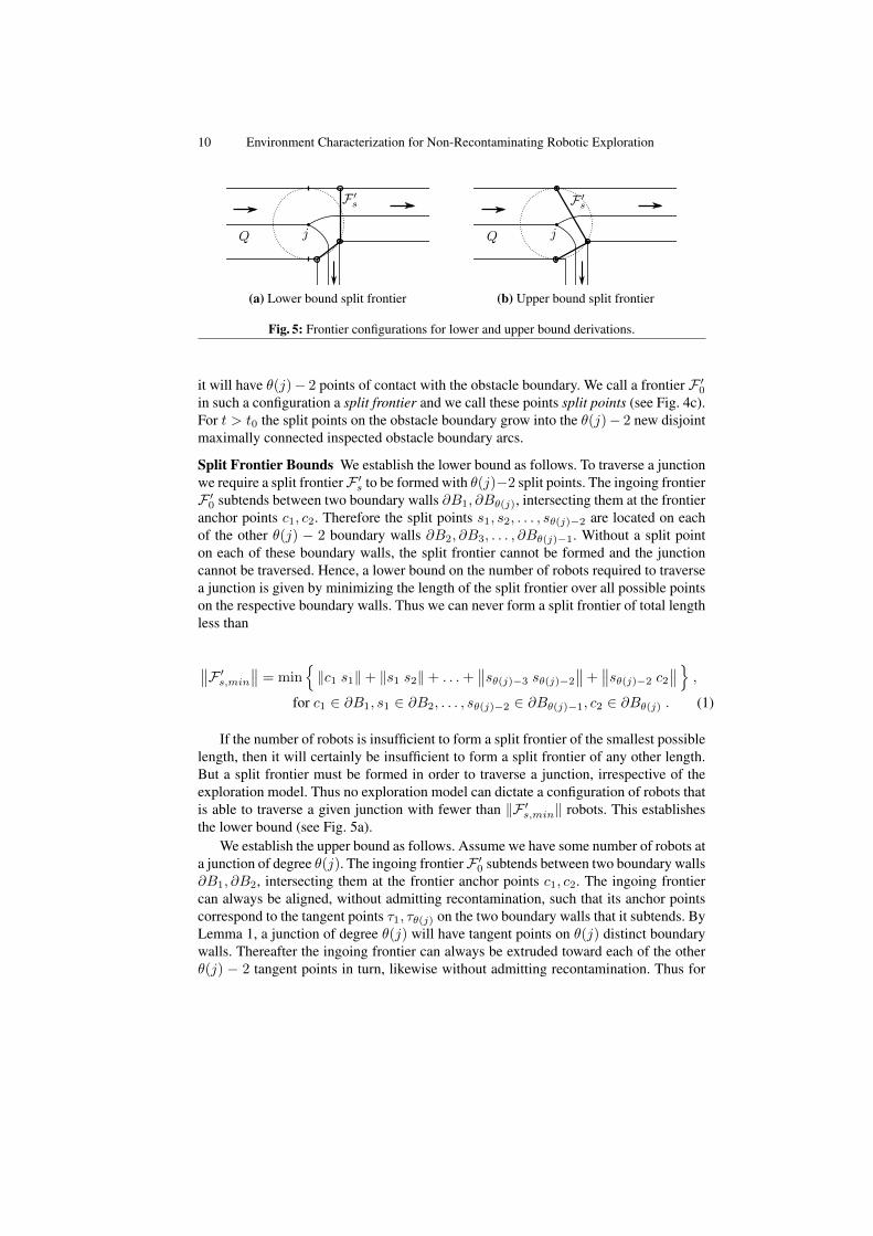
it will have θ(j)− 2 points of contact with the obstacle boundary. We call a frontier F ′0in such a configuration a split frontier and we call these points split points (see Fig. 4c).For t > t0 the split points on the obstacle boundary grow into the θ(j)− 2 new disjointmaximally connected inspected obstacle boundary arcs.

Split Frontier Bounds We establish the lower bound as follows. To traverse a junctionwe require a split frontierF ′s to be formed with θ(j)−2 split points. The ingoing frontierF ′0 subtends between two boundary walls ∂B1, ∂Bθ(j), intersecting them at the frontieranchor points c1, c2. Therefore the split points s1, s2, . . . , sθ(j)−2 are located on eachof the other θ(j) − 2 boundary walls ∂B2, ∂B3, . . . , ∂Bθ(j)−1. Without a split pointon each of these boundary walls, the split frontier cannot be formed and the junctioncannot be traversed. Hence, a lower bound on the number of robots required to traversea junction is given by minimizing the length of the split frontier over all possible pointson the respective boundary walls. Thus we can never form a split frontier of total lengthless than

∥∥F ′s,min∥∥ = min{‖c1 s1‖+ ‖s1 s2‖+ . . .+

∥∥sθ(j)−3 sθ(j)−2∥∥+ ∥∥sθ(j)−2 c2∥∥} ,for c1 ∈ ∂B1, s1 ∈ ∂B2, . . . , sθ(j)−2 ∈ ∂Bθ(j)−1, c2 ∈ ∂Bθ(j) . (1)

If the number of robots is insufficient to form a split frontier of the smallest possiblelength, then it will certainly be insufficient to form a split frontier of any other length.But a split frontier must be formed in order to traverse a junction, irrespective of theexploration model. Thus no exploration model can dictate a configuration of robots thatis able to traverse a given junction with fewer than ‖F ′s,min‖ robots. This establishesthe lower bound (see Fig. 5a).

We establish the upper bound as follows. Assume we have some number of robots ata junction of degree θ(j). The ingoing frontierF ′0 subtends between two boundary walls∂B1, ∂B2, intersecting them at the frontier anchor points c1, c2. The ingoing frontiercan always be aligned, without admitting recontamination, such that its anchor pointscorrespond to the tangent points τ1, τθ(j) on the two boundary walls that it subtends. ByLemma 1, a junction of degree θ(j) will have tangent points on θ(j) distinct boundarywalls. Thereafter the ingoing frontier can always be extruded toward each of the otherθ(j) − 2 tangent points in turn, likewise without admitting recontamination. Thus for


a junction j with tangent points τ1, τ2, . . . , τθ(j) we can always form a split frontier oftotal length

∥∥F ′s,max∥∥ = ‖c1 s1‖+ ‖s1 s2‖+ . . .+∥∥sθ(j)−3 sθ(j)−2∥∥+ ∥∥sθ(j)−2 c2∥∥

= ‖τ1 τ2‖+ ‖τ2 τ3‖+ . . .+∥∥τθ(j)−1 τθ(j)∥∥ . (2)

We can traverse any junction in this way, thus no junction will ever require morethan ‖F ′s,max‖ robots to traverse. This establishes the upper bound (see Fig. 5b). Ob-serve that since all the tangent points are on the boundary of a maximal inscribed circlecentered at j, the ingoing frontier F ′0, aligned such that its anchor points correspondto τ1, τθ(j), is at most 2D(j) in length, i.e. the diameter of the circle. For each of theθ(j) − 2 split points, the frontier gains an additional line segment, likewise of at most2D(j) in length. Thus we get a numeric upper bound on the maximum length of thesplit frontier, given by

∥∥F ′s,max∥∥ ≤ 2(θ(j)− 1

)D(j) . (3)

We have now established an equivalence between the medial axis configurationspace and the physical movement and frontier expansion of robots in physical space.We introduced an exploration model whereby a swarm locus moving along the skeletonallows us to reason about a group of robots moving through physical space. We definedwhat it means for a frontier to split and for a group of robots to traverse a junction, andderived lower and upper bounds on the number of robots required to traverse a junction.

4 Topology TreeIn this section we present a series of steps that will transform our continuous configura-tion space into a symbolic representation of the environment in the discrete domain. Weestablish a set of rules for navigating the environment in this discrete representation,that allow us to develop an algorithmic pursuit strategy. Using the junction lower boundfrom Result (1) we derive a lower bound on the total number of pursuers necessary toclear the environment, showing that no fewer than this number can possibly clear theenvironment regardless of the exploration model or pursuit strategy. Using the junctionupper bound from Result (2) we develop an upper bound on the total number of pur-suers that will always be sufficient to clear the environment, for any pursuit strategy.Finally, we derive an optimal pursuit strategy and prove that it guarantees we can clearthe environment with the minimum number of pursuers for a given exploration model.

The most natural representation of the skeleton of an environment where both Qand B are connected is a tree. Since we are also given a starting point on the skeleton,we consider a directed rooted tree (rooted at the start node). We refer to this as the en-vironment topology tree, denoted by T = (V,E), where V is the set of vertices (nodes)and E is the set of edges of T . Let s ∈ V be the root node of T . Nodes correspondto end points and junction points, and edges correspond to corridors connecting thesepoints on the skeleton.

Let γ : V → N denote the out-degree of a node. There are four types of nodes on thetopology tree. The swarm locus starts at an end point on the skeleton which corresponds


to the root node s of out-degree γ(s) = 1. Every other end point corresponds to a leafnode w of out-degree γ(w) = 0. Each junction point j is represented by a uniquejunction entry node u of out-degree γ(u) = θ(j)− 1, connected to an associated set ofdistinct junction exit nodes {v1, v2, . . . , vγ(u)} of out-degree γ(v) = 1. (Observe thatsince T is a directed rooted tree, every node has in-degree 1, except for the root node swhich has in-degree 0.)

The root node is connected to some junction entry node, while junction exit nodesare connected to leaf nodes and other junction entry nodes, as determined by the corri-dors connecting these points on the skeleton. Every edge e ∈ E on the topology tree isassigned a weight α : E → N. There are two fundamentally different types of edges:edges that represent a corridor on the skeleton and edges that represent the split frontierat a junction point.

Motivated by Corollary 1, for an edge e connecting node u of out-degree γ(u) = 1to a node v, the edge weight α(e) is determined by the number of robots necessary andsufficient to advance from u to v, given by the maximum relief value R(x) at somepoint x ∈ S amongst the points along that corridor.

Motivated by the reasoning in Section 3.2.2, for junction nodes the representationis as follows. For each junction entry node u ∈ V let Eu ⊂ E be the set of edges{e1, e2, . . . , eγ(u)} connecting u to its associated set of junction exit nodes {v1, v2, . . . ,vγ(u)}. For each junction, we define a traversal function δ : Eu → N, where

∑i δ(ei) is

the number of robots required to traverse the junction. This corresponds to the minimumnumber of robots required to form a split frontier at the junction, given by its ceilinglength d‖F ′s‖e. Since we do not have tight bounds on the length of the split frontier, thetraversal function depends on the the context of the analysis. Namely, if the goal is toderive a lower bound on the number of robots required to clear an environment, thenwe consider the length of the split frontier d‖F ′s,min‖e given by Result (1). If the goalis to derive an upper bound then we consider the length of the split frontier d‖F ′s,max‖egiven by Result (2). Each edge ei is assigned weight α(ei) = δ(ei) which correspondsto the number of robots ni that are are required to form a frontier F ′i at each outgoingcorridor, given by the ceiling length of each outgoing frontier d‖F ′i‖e.4.1 Exploration Rules

We consider exploration of the topology tree to be a game. We start the game with asingle group of n0 robots stationed at the root node s. Every node v ∈ V on the topologytree is marked with a label λ, which can have one of three values: CONTAMINATED,EXPLORED and CLEARED. Initially, the root node is marked EXPLORED and allother nodes are marked CONTAMINATED.

We play the game in rounds, each round moving some number of robots from onenode to another. If a group of robots is unable to move from one node to another on someround, then the robots are “stuck” at that node. This corresponds to the fact that if thereare insufficient robots to clear a corridor, they will remain stuck guarding the corridor,unable to retreat without allowing recontamination. Let λk(v) denote the labeling of anode v ∈ V on round k. We win the game if the tree is cleared on some round k0, thatis if ∃k0 ∈ N | ∀k > k0 ∀v ∈ V, λk(v) = CLEARED. We lose the game if all robotsare stuck at some node but the tree has not been cleared by some round k0, that is if∃k0 ∈ N | ∀k > k0 ∃v ∈ V, λk(v) 6= CLEARED.


Robots can split into smaller groups and join to form larger groups. In general, weare free to choose how we move the robots on the topology tree, provided that we obeythe following transition rules.

1. If a group of n0 robots reaches a node u where γ(u) > 0, then the group splits intosome permutation of γ(u) groups of ni robots advancing to each of the childrennodes {v1, v2, . . . , vγ(u)}. We are free to choose this permutation, subject to thefollowing restrictions:(a) If λ(vi) = CONTAMINATED, then ni ≥ α(ei(u)).(b) If λ(vi) = EXPLORED, then ni ≥ 0.(c) If λ(vi) = CLEARED, then ni = 0.If no such permutation exists, then the group remains stuck at node u.

2. If a group of robots is stationed at a node u where λ(u) = CLEARED, then thegroup backtracks to the parent node.

3. If a group of robots reaches a node u that is marked CONTAMINATED, then u ismarked EXPLORED.

4. If a group of robots reaches a leaf node u or a node u where all children of u aremarked CLEARED, then u is also marked CLEARED.

5. If two or more groups of n1, n2, . . . , nk groups of robots are stationed at the samenode, then they form a single group of n1 + n2 + . . .+ nk robots.

The reasoning behind these rules follows from the problem formulation and resultsin Section 3. Rule 1(a) enforces that our exploration is non-recontaminating. Rule 1(b)allows robots to move to explored nodes and join other robots. Rules 3 and 4 definethe progression of the game, and Rules 1(c) and 2 ensure that exploration is alwaysprogressive (the latter ensures a group of robots leaves a region once it has been cleared,while the former ensures that no group of robots re-enters that region unnecessarily).Rule 5 ensures that robots always act in a single group when stationed at a node.

We understand a state of the topology tree to mean the labeling of each node andthe number of robots stationed at each node on a given round. We call a sequence oftransitions between states of the topology tree a pursuit strategy. (We omit a formaldefinition for brevity.) A pursuit strategy is like a written record of a game of chessthat allows the game to be replayed by carrying out the recorded sequence of transi-tions. Observe that the only degree of freedom in choosing a pursuit strategy is whatto do at a given junction entry node u. We can always choose what junction exit nodeto send a group of robots to as long as it is not marked CLEARED. If the junctionexit nodes are marked CONTAMINATED then the group traverses the junction if andonly if n0 ≥

∑i α(ei(u)). If the junction is traversed, then the group splits into some

permutation of γ(u) groups of ni robots advancing to each of the associated junctionexit nodes {v1, v2, . . . , vγ(u)}. We are free to choose this permutation, provided that∀i, ni ≥ α(ei(u)). The choice we make in selecting this permutation may affect theoutcome of the game. (Note also that a node u is only marked CLEARED once the en-tire subtree T (u) is marked cleared. Thus robots are forced to clear subtrees recursively,and can only backtrack once a given subtree is cleared.)

We also note that because n0 and |V | are finite, there are a finite number of possiblepursuit strategies for a given topology tree. Intuition tells us that if n0 is too low, every


pursuit strategy will be a losing strategy, whereas if n0 is sufficiently high then anypursuit strategy will be a winning strategy. We now formalize this intuition, and derivelower and upper bounds on the total number of robots that can clear the topology tree.

4.2 Environment Bounds

Consider the topology tree T with root node s. Let T (q) be the tree obtained by con-sidering node q as the root node and removing nodes that are not descendants of q.Let n(T (q)) be the number of robots required to clear T (q). Let P (v) be the set ofnodes {p1, p2, . . . , pγ(v)} that are children of v ∈ V , enumerated in order of ascendingn(T (pi)).

We motivate the lower bound as follows. At each node s we consider whether morerobots are required to advance to the child node p1 than are required to clear the restof the subtree T (p1), and apply this recursively for the entire tree. At each junction en-try node we consider the maximum number of robots required to clear a given subtreeT (pi) while guarding the remaining junction exit nodes that have not been cleared. For-mally, let nmin(T (s)) be the total number of robots necessary to clear the environmentwith topology tree T , given by

nmin(T (s)) =0 if γ(s) = 0

max

{γ(s)∑i=1

α(ei(s)

), maxi=1,...,γ(s)

{nmin

(T (pi)

)+

γ(s)∑j=i+1

α(ej(s)

)}}otherwise .

(4)

Lemma 3. nmin(T (s)) robots are necessary to clear an environment with topologytree T , regardless of exploration model or pursuit strategy.

Proof. We begin at the root node s, which has out-degree γ(s) = 1. If α(e1(s)) >n(T (p1)), i.e. if more robots are required to advance to the child node p1 ∈ P (s) thanto clear the rest of the tree T (p1), then nmin(T (s)) = α(e1(s)). (The second term inthe outer max expression is not evaluated if γ(s) = 1.) This applies recursively forany node of out-degree γ(s) = 1. Leaf nodes provide the recursion base case, wheren(T (w)) = 0 for w ∈ V if γ(w) = 0.

For junctions the logic is as follows. For a junction entry node u ∈ V , each associ-ated junction exit node pi ∈ P (u) is the root node of a subtree T (pi). By Rules 1 and2, a group of robots that reaches a leaf node w will backtrack until it reaches a nodewith previously unexplored children. By induction a group of robots that clears T (pi)will backtrack until it returns to v and advance to a different junction exit node pj 6=i.By Rule 5, this group of robots will join with any other group of robots stationed at pj .When a group of robots reaches a junction, at least n0 >

∑i α(ei(u)) robots are re-

quired to traverse it thus stationing ni = α(ei(u)) robots at the γ(u) junction exit nodespi. Thereafter n0 must be at least enough to clear the subtree with smallest n(T (pi))while holding station at the remaining γ(u)− 1 exit nodes. This subtree is T (p1) sincepi ∈ P (u) are enumerated in order of ascending n(T (pi)). If n0 robots is not enough


to clear T (p1), then it will certainly not be enough to clear any other subtree, and thusthe junction cannot be traversed. If n0 robots is enough to clear T (p1) then n(T (p1))robots are now able to join one of the groups guarding the remaining γ(u)− 1 junctionexit nodes. We apply this iteratively for all subtrees T (pi), each time gaining the ser-vices of the group that cleared the previous subtree. The final subtree simply requiresn(T (pγ(u))) robots, since all other subtrees have been cleared and do not require anyrobots to guard the junction exit nodes. (Note that all ni groups of robots will actu-ally clear their subtrees simultaneously, in which case two given groups may not joinat the junction exit nodes, but elsewhere along a given subtree. However, consideringeach group to clear its subtree in stages with the other groups guarding the junctionexit nodes simplifies the abstraction.) We now consider the maximum of the numberof robots required to traverse the junction (the first term in the outer max expression)and the maximum number of robots required to clear a given subtree T (pi) and guardthe remaining γ(u) − i junction exit nodes (the second term in the outer max expres-sion, itself a maximum over γ(u) stages). The maximum of these two outer terms isthe minimum number of robots required to clear the subtree T (u). We apply this logicrecursively for all junctions.

Thus no fewer than nmin(T (s)) robots can clear an environment with topologytree T , for a given exploration model. Using the junction lower bound from Result (1)to obtain the traversal function δmin for each junction, we know that no fewer than∑i δmin(ei(u)) robots can traverse the junction point j corresponding to the junction

entry node u. Thus, using α(ei(u)) = δmin(ei(u)) for each junction entry point u,nmin(T (s)) gives a lower bound on the number of robots that is necessary to clear anenvironment with topology tree T , regardless of exploration model or pursuit strategy.

ut

We motivate the upper bound as follows. We imagine an adversary that dictates thepursuit strategy of a number of robots, with the goal of placing the maximum num-ber of them on the topology tree T , while preventing T from being cleared. Then weargue that given any such adversarial configuration of n?(T (s)) robots, n?(T (s)) + 1robots will always be able to clear T , regardless of the pursuit strategy chosen by theadversary. Formally, let nmax(T (s)) be the total number of robots sufficient to clear theenvironment with topology tree T , given by

nmax(T (s)) = n?(T (s)) + 1 ,

n?(T (s)) =

0 if γ(s) = 0

max

{( γ(s)∑i=1

α(ei(s)

))− 1 ,

γ(s)∑i=1

n?(T (pi)

)}otherwise .

(5)

Lemma 4. nmax(T (s)) robots are sufficient to clear an environment with topology treeT , for a given exploration model, regardless of pursuit strategy.

Proof. The adversary begins at the root node s, which has out-degree γ(s) = 1. Ifα(e1(s)) > n(T (p1)), i.e. if more robots are required to advance to the child node p1 ∈P (s) than to clear the rest of the tree T (p1), then n?(T (s)) simply equals α(e1(s))− 1


since adding one more robot will result in the entire tree being cleared. This appliesrecursively for any node of out-degree γ(s) = 1. Leaf nodes provide the recursion basecase, where n(T (w)) = 0 for w ∈ V if γ(w) = 0.

For junctions the logic is as follows. For a junction entry node u ∈ V , each asso-ciated junction exit node pi ∈ P (u) is the root node of a subtree T (pi). The adversarycan choose one of two options: either place

(∑γ(s)i=1 α(ei(s))

)− 1 robots at u such that

the junction cannot be traversed, or traverse the current junction with∑γ(s)i=1 n

?(T (pi)

)robots knowing that they will not be able to clear the rest of the tree. The adversarychooses the maximum of these two values since she is trying to maximize the numberof robots on the tree. We apply this logic recursively for all junctions.

Consider any such configuration of n?(T (s)) robots. We now introduce one ad-ditional robot at the root node s. The robot must navigate the tree according to theexploration rules, but the adversary is still free to choose its pursuit strategy. By Rule 5,whenever the robot reaches any node u with n?(T (u)) robots stationed at the node, asingle group of n?(T (u)) + 1 robots forms at u which is sufficient to clear the subtreeT (u). By Rule 2, any group of robots that clears a subtree will backtrack along the treeuntil it reaches a previously unexplored part of the tree. This group of robots will joinother groups of n?(T (v)) robots similarly stationed at other nodes v ∈ V . This willcontinue recursively until the entire tree is cleared. Thus placing an additional robotat s causes a “chain reaction” that results in T being cleared regardless of the pursuitstrategy that the adversary chooses for any of the n?(T (s)) + 1 robots.

Thus no more than nmax(T (s)) = n?(T (s))+1 robots will ever be required to clearan environment with topology tree T , regardless of pursuit strategy. Using the junctionupper bound from Result (2) to obtain the traversal function δmax for each junction, weknow that no more than δmax(ei(u)) robots are required to traverse the junction point jcorresponding to the junction entry node u for the given exploration model. Thus, usingα(ei(u)) = δmax(ei(u)) for each junction entry point u, nmax(T (s)) gives an upperbound on the number of robots that is sufficient to clear an environment with topologytree T , for a given exploration model, regardless of pursuit strategy. ut

4.3 Optimal Pursuit Strategy

We now present an optimal pursuit strategy that guarantees that the environment iscleared with the minimum number of robots for a given exploration model. Considerthe topology tree T with root node s. We know that nmin(T (s)) robots are necessary toclear T , given by Result (4). The following algorithm guarantees that T will be clearedwith nmin(T (s)) robots. (We use the same notation as in Section 4.2.)

Algorithm 1 – Clear(T (s), n0

)Given n0 robots located at root node s of topology tree T = (V,E):

1. If s is a leaf node or if all children of s are marked CLEARED, then:(a) mark s← CLEARED.(b) Backtrack to parent node. If parent node does not exist, terminate.

2. If λ(s) = CONTAMINATED, mark s← EXPLORED.3. If γ(s) = 1, Clear

(T (p1), n0

).


4. If γ(s) > 1 and if all children of s are marked CONTAMINATED, then:(a) for i = 2, . . . , γ(s): Clear

(T (pi), α(ei(s))

).

(b) Clear(T (p1), n0−

∑γ(s)i=2 α(ei(s))

).

5. If γ(s) > 1 and if all children of s are not marked CONTAMINATED, then:(a) let i = min2,...,γ(s)

{i | λ(pi) 6= CLEARED

}.

(b) Clear(T (pi), n0

).

Lemma 5. nmin(T (s)) robots are necessary and sufficient to clear an environmentwith topology tree T , for a given exploration model.

Proof. Given nmin(T (s)) robots we prove that we can use the Clear algorithm toclear the environment. Let n0 = nmin(T (s)). We begin at the root node s, which hasout-degree γ(s) = 1. A group of robots can always advance to the child node p1 sincewe have n0 = nmin(T (s)) robots. This applies for all nodes of out-degree γ(s) = 1.When a group of robots reaches a leaf node it is marked CLEARED. A group of robotsstationed at a node that is marked CLEARED will backtrack until it reaches a node withchildren that are not marked CLEARED.

For junctions, the logic is as follows. The first time a group of robots reaches agiven junction entry node u, all children of u are marked CONTAMINATED. We sendni = α

(ei(s)

)robots to each of the γ(s) − 1 junction exit nodes pi, and use the

remaining n1 = n0 −∑γ(s)i=2+1 α

(ei(s)

)robots to clear the subtree T (p1). By proof

to Lemma 3, we know that the entire subtree T (p1) can be cleared with n1 robots,and therefore n1 robots will eventually backtrack to u. Thereafter, all children of u areeither EXPLORED or CLEARED. Each group of robots reaching u in this way is sentto clear T (pi) where i is the smallest number such that λ(i) 6= CLEARED. We do thisiteratively for each subtree, each time gaining the services of the group that clearedthe previous subtree. We can always clear each subtree T (pi) in this manner because{p1, p2, . . . , pγ(v)} are enumerated in order of ascending n(T (pi)), and by proof toLemma 3 we know that n(T (u)) robots is enough to clear every subtree in this way.For each subtree T (pi) cleared in this way, pi is marked CLEARED. When all subtreeshave been cleared, u will be marked CLEARED, and the entire group of robots willbacktrack to the parent node. This applies recursively recursively for all junctions. ut

Using the junction upper bound from Result (2) to obtain the traversal functionδmax for each junction, we know that no more than δmax(ei(u)) robots are required totraverse the junction point j corresponding to the junction entry node u for the givenexploration model. Thus, using α(ei(u)) = δmax(ei(u)) for each junction entry pointu, the Clear algorithm gives an optimal pursuit strategy for clearing an environmentwith topology tree T , for a given exploration model.

5 ConclusionThe problem of obtaining a concise characterization of a physical environment in thecontext of frontier-based non-recontaminating exploration was considered. We intro-duced the medial axis as a configuration space and showed that reasoning about pointsin this configuration space is equivalent to reasoning about robots in physical space.


We formalized the notion of width, corridors and junctions and derived lower and up-per bounds on the number of robots required to traverse a junction. We presented atransformation from this continuous configuration space into a symbolic representationin the discrete domain. We cast the exploration problem as a game, established rulesfor playing this game, and derived bounds on the number of robots necessary and suf-ficient to clear the environment. Finally we presented an optimal pursuit strategy thatguarantees that we can clear the environment with the minimum number of robots.

There are a number of interesting future lines of research for this work. First, theestablishment of tight bounds on the number of robots required to traverse a junction —we suspect that the lower bound given by Result (1) in Section 3.2 is in-fact necessaryand sufficient. A rigorous proof of this fact would have to generalize to accommodate anumber of special cases.

Second, the extension of this work to environments with holes would be a signif-icant contribution. The medial axis configuration space was chosen with this in mind,and the model presented in Section 3 soundly generalizes the characterization to arbi-trary connected environments. A number of issues need to be addressed in transformingthis representation into the discrete domain. One would need to consider an undirectedgraph and junctions would need to be represented accordingly. It is known that comput-ing the number of searchers required to clear a general graph is NP-hard [21], so suitableheuristics or approximations would need to be employed. Alternatively, the graph couldbe converted into a tree such as in [15], [16]; however the non-isotropic nature of thejunction transition function would demand a judicious approach to blocking cycles.

Acknowledgements This research was supported in part by the Future Urban Mo-bility project of the Singapore-MIT Alliance for Research and Technology (SMART)Center, with funding from Singapore’s National Research Foundation. It was also sup-ported in part by AFOSR Award Number FA9550-08-1-0159, NSF Award NumberCNS-0715397, NSF Award Number CCF-0726514, ONR grant N000140911051 andNSF grant 0735953. We are grateful for this support.

References1. M. Adler, H. Racke, N. Sivadasan, C. Sohler, and B. Vocking. Randomized pursuit-evasion

in graphs. Combinatorics, Probability and Computing, 12(03):225–244, 2003.2. H. Blum. A transformation for extracting new descriptors of shape. Models for the Perception

of Speech and Visual Form, 19:362–380, 1967.3. J. Burgos. Pursuit/evasion behaviors for multi-agent systems. 2010.4. H. Choi, S. Choi, and H. Moon. Mathematical theory of medial axis transform. Pacific

Journal of Mathematics, 181(1):57–88, 1997.5. P. Danielsson. Euclidean distance mapping. Computer Graphics and image processing,

14(3):227–248, 1980.6. P. Dimitrov, C. Phillips, and K. Siddiqi. Robust and efficient skeletal graphs. In cvpr, page

1417. Published by the IEEE Computer Society, 2000.7. J. Durham, A. Franchi, and F. Bullo. Distributed pursuit-evasion with limited-visibility sen-

sors via frontier-based exploration. In Robotics and Automation (ICRA), 2010 IEEE Inter-national Conference on, pages 3562–3568. IEEE, 2010.

8. B. Gerkey, S. Thrun, and G. Gordon. Visibility-based pursuit-evasion with limited field ofview. The International Journal of Robotics Research, 25(4):299, 2006.


9. P. J. Giblin and B. B. Kimia. Local forms and transitions of the medial axis. In K. Siddiqiand S. M. Pizer, editors, Medial Representations, volume 37 of Computational Imaging andVision, pages 37–68. Springer Netherlands, 2008.

10. L. Guibas, C. Holleman, and L. Kavraki. A probabilistic roadmap planner for flexible objectswith a workspace medial-axis-based sampling approach. In Intelligent Robots and Systems,1999. IROS’99. Proceedings. 1999 IEEE/RSJ International Conference on, volume 1, pages254–259. IEEE, 1999.

11. L. Guibas, J. Latombe, S. Lavalle, D. Lin, and R. Motwani. Visibility-based pursuit-evasionin a polygonal environment. Algorithms and Data Structures, 1272:17–30, 1997.

12. L. Guibas, J. Latombe, S. LaValle, D. Lin, and R. Motwani. A visibility-based pursuit-evasion problem. International Journal of Computational Geometry and Applications,9(4/5):471, 1999.

13. C. Holleman and L. Kavraki. A framework for using the workspace medial axis in prmplanners. In Robotics and Automation, 2000. Proceedings. ICRA’00. IEEE InternationalConference on, volume 2, pages 1408–1413. IEEE, 2000.

14. V. Isler, D. Sun, and S. Sastry. Roadmap based pursuit-evasion and collision avoidance. InProc. Robotics, Systems, & Science, 2005.

15. A. Kolling and S. Carpin. The graph-clear problem: definition, theoretical properties and itsconnections to multirobot aided surveillance. In Intelligent Robots and Systems, 2007. IROS2007. IEEE/RSJ International Conference on, pages 1003–1008. IEEE, 2007.

16. A. Kolling and S. Carpin. Multi-robot surveillance: an improved algorithm for the graph-clear problem. In Robotics and Automation, 2008. ICRA 2008. IEEE International Confer-ence on, pages 2360–2365. IEEE, 2008.

17. A. Kolling and S. Carpin. Pursuit-evasion on trees by robot teams. Robotics, IEEE Transac-tions on, 26(1):32–47, 2010.

18. A. Kuijper. Deriving the medial axis with geometrical arguments for planar shapes. PatternRecognition Letters, 28(15):2011–2018, 2007.

19. S. LaValle, D. Lin, L. Guibas, J. Latombe, and R. Motwani. Finding an unpredictable targetin a workspace with obstacles. In Robotics and Automation, 1997. Proceedings., 1997 IEEEInternational Conference on, volume 1, pages 737–742. IEEE, 1997.

20. R. Nowakowski and P. Winkler. Vertex-to-vertex pursuit in a graph. Discrete Mathematics,43(2-3):235–239, 1983.

21. T. Parsons. Pursuit-evasion in a graph. Theory and applications of graphs, 642:426–441,1978.

22. S. Rodriguez, J. Denny, T. Zourntos, and N. Amato. Toward simulating realistic pursuit-evasion using a roadmap-based approach. Motion in Games, 6459:82–93, 2010.

23. S. Sachs, S. LaValle, and S. Rajko. Visibility-based pursuit-evasion in an unknown planarenvironment. The International Journal of Robotics Research, 23(1):3, 2004.

24. J. Serra. Image analysis and mathematical morphology. London.: Academic Press.[Reviewby Fensen, EB in: J. Microsc. 131 (1983) 258.] Technique Staining Microscopy, Reviewarticle General article, Mathematics, Cell size (PMBD, 185707888), 1982.

25. I. Suzuki and M. Yamashita. Searching for a mobile intruder in a polygonal region. SIAMJournal on computing, 21:863, 1992.

26. S. Wilmarth, N. Amato, and P. Stiller. Maprm: A probabilistic roadmap planner with sam-pling on the medial axis of the free space. In Robotics and Automation, 1999. Proceedings.1999 IEEE International Conference on, volume 2, pages 1024–1031. IEEE, 1999.

27. M. Yamashita, H. Umemoto, I. Suzuki, and T. Kameda. Searching for mobile intruders in apolygonal region by a group of mobile searchers. Algorithmica, 31(2):208–236, 2001.

28. B. Yamauchi. A frontier-based approach for autonomous exploration. In ComputationalIntelligence in Robotics and Automation, 1997. CIRA’97., Proceedings., 1997 IEEE Interna-tional Symposium on, pages 146–151. IEEE, 1997.


29. B. Yamauchi. Frontier-based exploration using multiple robots. In Proceedings of the secondinternational conference on Autonomous agents, pages 47–53. ACM, 1998.

Environment Characterization for Non-Recontaminating ... · Environment Characterization for...

Documents

Transcript of Environment Characterization for Non-Recontaminating ... · Environment Characterization for...