Entrepreneurship, wealth inequality, and taxation€¦ · Entrepreneurship, wealth inequality, ......
32
Review of Economic Dynamics 8 (2005) 688–719 www.elsevier.com/locate/red Entrepreneurship, wealth inequality, and taxation ✩ Césaire A. Meh Department of Monetary and Financial Analysis, Bank of Canada, 234 Wellington, Ottawa, Ontario, Canada K1A 0G9 Received 19 June 2003 Available online 13 June 2005 Abstract This paper investigates the importance of entrepreneurship when quantifying the aggregate and distributional effects of switching from a progressive to a proportional income tax system. I find that the distributional consequences of the tax reform in a model economy with entrepreneurs contrast markedly from those in a model economy with no entrepreneurs. The elimination of progressive taxation has a negligible effect on wealth inequality when entrepreneurship is considered but has a large effect when entrepreneurship is omitted. The framework used is an occupational choice model, in which the decision to become an entrepreneur is determined by the ability to manage a firm and by asset holdings. The calibrated economy can account for the high savings rate of entrepreneurs relative to non-entrepreneurs, and the high concentration of wealth observed in the data. 2005 Elsevier Inc. All rights reserved. JEL classification: D31; E62; H23; H20 Keywords: Entrepreneurship; Distribution of wealth; Progressive taxation; Proportional taxation; Financial constraints 1. Introduction In this paper, I investigate the extent to which entrepreneurship is important in quanti- fying the aggregate and distributional effects of switching from a progressive to a propor- ✩ This paper is a revised version of Chapter 2 of my PhD dissertation at the University of Western Ontario. The views expressed herein are those of the author and not necessarily those of the Bank of Canada. E-mail address: [email protected]. 1094-2025/$ – see front matter 2005 Elsevier Inc. All rights reserved. doi:10.1016/j.red.2005.03.001
Transcript of Entrepreneurship, wealth inequality, and taxation€¦ · Entrepreneurship, wealth inequality, ......
d
ate andd thatontrastessivet has amodel,
rm andreneurs
l
uanti-opor-
io. The
Review of Economic Dynamics 8 (2005) 688–719
www.elsevier.com/locate/re
Entrepreneurship, wealth inequality, and taxation✩
Césaire A. Meh
Department of Monetary and Financial Analysis, Bank of Canada, 234 Wellington, Ottawa,Ontario, Canada K1A 0G9
Received 19 June 2003
Available online 13 June 2005
Abstract
This paper investigates the importance of entrepreneurship when quantifying the aggregdistributional effects of switching from a progressive to a proportional income tax system. I finthe distributional consequences of the tax reform in a model economy with entrepreneurs cmarkedly from those in a model economy with no entrepreneurs. The elimination of progrtaxation has a negligible effect on wealth inequality when entrepreneurship is considered bularge effect when entrepreneurship is omitted. The framework used is an occupational choicein which the decision to become an entrepreneur is determined by the ability to manage a fiby asset holdings. The calibrated economy can account for the high savings rate of entreprelative to non-entrepreneurs, and the high concentration of wealth observed in the data. 2005 Elsevier Inc. All rights reserved.
JEL classification: D31; E62; H23; H20
Keywords: Entrepreneurship; Distribution of wealth; Progressive taxation; Proportional taxation; Financiaconstraints
1. Introduction
In this paper, I investigate the extent to which entrepreneurship is important in qfying the aggregate and distributional effects of switching from a progressive to a pr
✩ This paper is a revised version of Chapter 2 of my PhD dissertation at the University of Western Ontarviews expressed herein are those of the author and not necessarily those of the Bank of Canada.
E-mail address: [email protected].
1094-2025/$ – see front matter 2005 Elsevier Inc. All rights reserved.doi:10.1016/j.red.2005.03.001
C.A. Meh / Review of Economic Dynamics 8 (2005) 688–719 689
and1991),of taxirst,
.tion.nt and
x rates.ontrastnal in-isions
venueentre-ct on
repre-are ofevious
d that amea-
neurs,se by
easesate out-
es withe im-xation
r thers andadrinibusi-
llectioncus on
trepre-ic growth
(1998),
tional income tax system.1 While the relationship between entrepreneurship, inequalitytaxation has been examined qualitatively (e.g., Kanbur, 1982 and Boadway et al.,entrepreneurship has been omitted in most quantitative general-equilibrium studiespolicy.2 Such an omission is likely to be significant for the following three reasons. Fentrepreneurship is often considered as a key source of job and economic growth3 Sec-ond, entrepreneurship is important in explaining wealth accumulation and its distribu4
Third, entrepreneurial decisions (such as entrepreneurial entry, savings, investmechanges in the scale of businesses) are greatly affected by progressive marginal ta5
To address the relationship between entrepreneurship, inequality and taxation, I cthe steady-state implications of moving from progressive to equal-revenue proportiocome taxation in two distinct model economies: one in which entrepreneurship decare modelled, and another that does not account for entrepreneurial activity.6
The main finding of the analysis is that switching from a progressive to an equal-reproportional income tax system has only a small impact on wealth inequality whenpreneurship is explicitly modelled, while the same policy change has a large effewealth inequality in an economy with no entrepreneurs. In the economy without entneurs, the Gini index of the distribution of wealth increases by 9.5 percent and the shwealth held by the top 5 percent increases by 11.3 percent. This is consistent with prresearch which omits entrepreneurship. For instance, Castañeda et al. (1999) finswitch to proportional income taxation substantially increases wealth inequality, assured by the Gini index, by 10.5 percent. By contrast, in the economy with entreprethe wealth Gini coefficient and the share of wealth held by the top 5 percent increaonly 1.4 and 4.3 percent, respectively.
I also find that the change from progressive to proportional income taxation incrcapital accumulation, entrepreneurial investments and savings, and therefore aggregput. The increases in capital accumulation and aggregate output—in both economiand without entrepreneurs—are in line with findings of the literature that explores thpact of replacing the current US progressive income tax system by other forms of ta(such as flat tax and proportional income tax).7
To arrive at these findings I use two models that can quantitatively account fohigh concentration of wealth observed in the US data: the model with entrepreneuthe model without entrepreneurs. First, the model with entrepreneurs is built on Qu(2000), who uses a calibrated general-equilibrium framework to show that modelling
1 Entrepreneurship is defined as business ownership.2 See Castañeda et al. (1999), Altig and Carlstrom (1999), Altig et al. (2001), and most papers in the co
edited by Aaron and Gale (1996). None of these quantitative general-equilibrium studies of tax policy foentrepreneurship.
3 See Haltiwanger and Krizan (1999) and Bednarzik (2000) for the link between job growth and enneurship, and Schumpeter (1934) and Banerjee and Newman (1993) for the entrepreneurship-economnexus.
4 See Quadrini (1999) and Gentry and Hubbard (1999).5 See Carroll et al. (1998a, 1998b) and Gentry and Hubbard (2000a, 2000b).6 I have embarked on a research program on entrepreneurial activity and taxation in Meh (2001).7 This result is consistent with the findings of Altig et al. (2001), Castañeda et al. (1999), Heckman et al.
Sarte (1997) and Ventura (1999), among others.
690 C.A. Meh / Review of Economic Dynamics 8 (2005) 688–719
r,ing a. In thes busi-chastict man-eurialch antrepre-higher
ks as-eouslytrationto theortuni-used
o match
e taxduces
r, thusr. As aithoutdel en-wealthpaids to in-lementsstmentrivingorkers.orkers
er andlt isd en-
ates are,d Smithutionale models-cycle
odel.
ness ownership can explain the high concentration of wealth.8 Unlike the present papeQuadrini (2000) does not consider tax reform issues. I extend his model by includgovernment sector that collects tax revenues via a progressive income tax systemmodel, the decision to undertake entrepreneurial activity is determined by the agent’ness ability and his net worth. The ability to manage a business is modelled as a stoprocess where agents gradually acquire the ability to run larger businesses by firsaging smaller ones. Net worth is important in the decision to undertake entreprenactivity because of borrowing constraints and financial intermediation costs. In suenvironment progressive income taxation reduces the incentives to become an enneur, since business ownership promotes income growth and moves the agent to atax bracket. Because of borrowing constraints, costly external financing, and the rissociated with business ownership, the calibrated model is able to account simultanfor the high savings rate of entrepreneurs relative to workers and the high concenof wealth observed in the data. Second, the model without entrepreneurs is similarmodel with entrepreneurs, except that households do not have entrepreneurial oppties. To account for the observed high concentration of wealth, I follow the approachby Castañeda et al. (2003), where the stochastic process of earnings is calibrated tthe observed distribution of wealth.
In the model with entrepreneurs, replacing a progressive by a proportional incomsystem has two opposing effects. First, the switch to proportional income taxes rethe marginal income tax rate for wealthy households, but increases it for the pooincreasing the incentive to save faced by the wealthy and decreasing it for the pooresult, wealth inequality increases. This effect, which is also present in the model wentrepreneurs, has traditionally been emphasized in previous studies that do not motrepreneurship. The second effect, which is the main focus of this paper, decreasesinequality following the tax reform. The reduction in the marginal income tax ratesby entrepreneurs—as entrepreneurs are mostly located in higher tax brackets—leadcreased entrepreneurial investments and savings. Since labor and capital are compin the production technology used by entrepreneurs, the increased business inveboosts the demand for labor, which, in turn, increases the wage rate, effectively ddown the average return to entrepreneurial activities and increasing the income of wThis general-equilibrium feedback narrows the income and savings gap between wand entrepreneurs, leading to a reduction in income and wealth inequality.9 In the quan-titative findings presented above, these two effects approximately offset each oththe overall wealth inequality increases only slightly. A crucial factor driving this resuthe presence of borrowing constraints and costly financial intermediation, which lea
8 Other models that have been able to replicate the observed concentration of wealth in the United Stfor example, Castañeda (1999, 2003), Cagetti and De Nardi (2002), De Nardi (2000), and Krussel an(1998). See Quadrini and Ríos-Rull (1997) and Castañeda (2003, pp. 5–7) for an overview of the distribconsequences of economies with heterogeneous agents in terms of the distribution of wealth. Most of thesare either extensions of Aiyagari (1994)—an infinitely lived agents economy—or Huggett (1996)—a lifeeconomy.
9 This general-equilibrium feedback has been put forward qualitatively by Kanbur (1982) in a static m
However, the effect has not been quantified.
C.A. Meh / Review of Economic Dynamics 8 (2005) 688–719 691
whicheurs are
quan-it issavingstax re-
ressivetchingynastic
a dy-wealthmansolelyeurial
Gen-olicy
ion and
modelesent angs ofs.
e oned thenomy isd, theet. Thenment.
y. Holtz-arental
choicepends ono study
count for
trepreneurs to operate at a sub-optimal scale. The reduction in marginal tax rates—increases entrepreneurial savings—relaxes the borrowing constraints and entreprenable to expand production and employ more capital and labor.10
The above findings suggest the importance of considering entrepreneurship whentifying the aggregate and distributional effects of tax policy. To put it differently,necessary to account for entrepreneurial decisions (such as entrepreneurial entry,and investments) when measuring the trade-off between efficiency and equality offorms.
Other researchers have quantified the effects of replacing the current US progincome tax system with a proportional tax. Perhaps, the closest (in terms of mainequality when looking at tax issues) are Castañeda et al. (1999) who use a dmodel with exogenous human capital, and Erosa and Koreshkova (2003) who usenastic model with endogenous human capital. They find a substantial increase ininequality after the elimination of progressive taxation. Altig et al. (2001) and Hecket al. (1998) use an overlapping generation framework in which savings are drivenby life-cycle motives. However, none of these models consider the role of entreprenactivity.
There is a large literature studying the effects of taxation on entrepreneurship.try and Hubbard (2000b, Section 2, pp. 2–7) provide an excellent overview of tax pand entrepreneurship. None of the models surveyed there examine inequality, taxatentrepreneurship in a unified framework.11
The remainder of the paper is organized as follows. Section 2 first describes thewith entrepreneurs and then the model without entrepreneurs. Sections 3 and 4 prdescription of the calibration and the calibration results. Section 5 presents the findithe tax reform. Section 6 provides some sensitivity analysis, and Section 7 conclude
2. Model with entrepreneurs
Given that the description of the model with entrepreneurs is roughly similar to thof the model without entrepreneurs I mainly present the model with entrepreneurs andiscuss the model without entrepreneurs at the end of the section. The model econpopulated by a continuum of infinitely lived households of measure one. In each perioagents decide whether to run a business or to supply their labor service to the markeconomy consists of four sectors: household, production, intermediation, and gover
10 Gentry and Hubbard (1999) show that external financing to start and expand a business is very costlEakin et al. (1994a, 1994b) show that the probability of becoming an entrepreneur increases with pinheritance of wealth. These facts indicate the importance of borrowing constraints in entrepreneurship.11 Gravelle and Kotlikoff (1989, 1995) study the welfare effects of corporate taxation in an occupationalmodel where the decision to become an entrepreneur—who operates in the non-corporate sector—dethe agent’s business ability, but not on his net worth. In a recent paper, Cagetti and De Nardi (2004) alsentrepreneurship, estate and income taxation, but they use a different modelling strategy and do not ac
the wage effect on entrepreneurship which turns out to be important for the present paper.
692 C.A. Meh / Review of Economic Dynamics 8 (2005) 688–719
ent be-lt, for
with a
al idea,
ich
tediod.ve anerly, it isfor thed, that
ses hishnologyhe samet change.t becom-n to theate labor
urs (evenge ratethis maytion.Evans,
2.1. Household sector
2.1.1. Preferences and labor efficienciesHouseholds maximize their expected discounted lifetime utility:
E0
{ ∞∑t=0
βtu(ct )
}, (1)
E0 is the expectation operator conditional on information at date 0,ct is consumption, andβ is the discount factor, where the momentary utility is given:
u(c) = c1−σ
1− σ.
In each period, households are endowed withε ∈ {ε1, . . . , εNε } units of labor efficien-cies, which can either be supplied to the market in return for the wage rate,ω, or be directlyemployed in its own business. I assume that an entrepreneurial household is indiffertween employing its own labor service and hiring labor from the market. As a resusimplicity, the household is assumed to supply all its labor to the market.12 The labor effi-ciency is observed at the end of the period and follows a first-order Markov processtransition probabilityΓ (ε′, ε).
2.1.2. Entrepreneurial ideasThe household can also run a business project by implementing an entrepreneuri
k, drawn at the end of each period from the setK = {k0, k1, . . . , kNk}, whereki−1 < ki for
i = 1, . . . ,Nk. The first element ofK is set atk0 = 0 and corresponds to the case in whthere is no entrepreneurial idea and the household is a worker.
The entrepreneurial idea,k, is a random variable with a probability distribution denoby Pk(k), where the subscriptk denotes the project implemented in the current perMore precisely,Pki
(k) describes a “learning” process that requires the agent to haidea,ki, before receiving an idea,ki+1.13 In other words, the probability of getting bettentrepreneurial ideas increases if the agent is running better projects. Specificalassumed, on the one hand, that the probability of a new better idea is positive onlynext-highest project close to the one that is currently being run, and, on the other han
12 It is worth noting the following two elements. First, it can also be assumed that the entrepreneur ulabor to manage the business and that his only source of income is profits. If the structure of the tecin the entrepreneurial sector is appropriately modified, the total income of the entrepreneur can have tproperties as the one he earns in the current version of the paper. And consequently, the results would noOne advantage of assuming that entrepreneurs retain their labor income is that it is easier to see thaing entrepreneurs increases income risks since it brings another source of income uncertainty in additiouncertainty in labor income. Second, if the entrepreneur uses his labor to manage the business, aggregsupply will be endogenous since it is determined by moves between the pools of workers and entreprenethough labor supply is inelastic at the individual level). This mechanism may imply a greater rise in the wawhen entrepreneurs increase their demand for labor after the elimination of progressive taxation. Thusreinforce the main result of the paper regarding the distributional effects of switching to proportional taxa13 This is consistent with the observation that on average “younger” firms are smaller than “older” firms (
1987).
C.A. Meh / Review of Economic Dynamics 8 (2005) 688–719 693
. As a
n ale-d of the
ntre-essump-eurial
n.
neur.s: thesurablees thatl sector
rved
withs
set of
the implemented project in the present period can always be run by the householdresult, for all current business projects,ki , wherei = 0, . . . ,Nk, the probability distributionis such that
Pki(k)
> 0 if k ∈ {ki, ki+1} andi < Nk,
= 1 if k = ki andi = Nk,
= 0 otherwise.
(2)
Given the definition ofPk(k), the set of projects with which the household can rubusiness in the next period is given by{k, k}, where the first element is the project impmented in the current period and the second element is the idea obtained at the enperiod.
Finally, I assume that the amount of capital required for the realization of an epreneurial project is indivisible. In other words, if the household wants to run a businproject, it has to invest the fixed amount of capital required by that project. This asstion, coupled with the fact that the set of ideas is discrete, implies that the entreprenidea,k, is characterized by the amount of capital input required for its implementatio
2.2. Production sector
In reality, not all firms (particularly large firms) are managed by a single entrepreTherefore, in the model there is one good which is produced by two distinct sectornon-entrepreneurial sector and the entrepreneurial sector. In this paper, the uninentrepreneurial risk and the strictness of financial constraints are the main featurcharacterize and differentiate the entrepreneurial sector from the non-entrepreneuria(in the spirit of Fazzari et al., 1988, and Gertler and Gilchrist, 1994).
2.2.1. Entrepreneurial sectorThe production function associated with a project,k, is given by
f (z, k, n) = zνkνn1−ν, (3)
whereν ∈ (0,1) is the capital income share,n is the number of efficiency units of laboinput, andz ∈ Zk = {z1k, . . . , zNzk} is an idiosyncratic technology shock that is obserat the beginning of the current period and that follows a first-order Markov processtransition probabilityQk(z
′, z). The set from which the shock,z, takes values, as well aits probability distribution, depends on the implemented project,k. The first element of theset,Zk , is assumed to be a bad shock that is highly persistent; i.e.,Qk(z1k, z1k) = 1. As aresult, if entrepreneurs receive it, they will exit from entrepreneurship.
The production plan in this sector is determined as follows:
(i) at the end of the period, the entrepreneur decides which project to run from theimplementable projects, and
(ii) at the beginning of the next period, after observing the technological shock,z, the
entrepreneur decides how much labor to use in production.
694 C.A. Meh / Review of Economic Dynamics 8 (2005) 688–719
ock,
ief thatneurialeivesvalue
rge
wing
reciates
sitiveon-
e non-g com-
.t theanyentriod,
d
d
Hence, running a business project,k, in the current period means that its requiredk unitsof capital input had to be invested in the previous period before the technological shz,is observed, while the labor input,n, is chosen after the observation ofz.
Finally, the amount of capital invested depreciates stochastically, based on the belthe end-of-period value of the invested capital depends on the result of the entrepreactivity (which is the realization of the technological shock). If the entrepreneur reca good shock, the value of the invested capital is high; if the shock is bad, then theof the invested capital is low. The depreciation rate is denoted byδz, and it is a function ofthe shock,z. The introduction of stochastic depreciation allows for the possibility of lalosses in entrepreneurial activities.
2.2.2. Non-entrepreneurial sectorThe production function in the non-entrepreneurial sector is given by the follo
constant returns-to-scale production function:
F(Kc,Nc) = Kθc N1−θ
c , (4)
whereθ is the capital income share in the non-entrepreneurial sector,Kc, andNc are theaggregate capital and labor efficiencies used in this sector, respectively. Capital depat rateδ.14
2.3. Intermediation sector and borrowing constraints
In the model economy, intermediaries collect deposits from households with pobalances (by paying the interest rate,rd ) to lend those funds to households and the nentrepreneurial sector. While there is a positive proportional cost,γ , per unit of fundsintermediated to households undertaking entrepreneurial activities, loans made to thentrepreneurial sector use no resources. Given the large number of banks behavinpetitively, bank profits are zero. This assumption implies that the lending rate equalsrd forloans to the non-entrepreneurial sector andrl = rd + γ for loans to the household sector
The lending policy for intermediaries consists of lending up to the amount thaborrower will be able to repay with certainty at the end of the following period. Forgiven projectk ∈ K, let zmin be the lowest possible realization of the shock. If the agdevotesk units of capital in the project, then the minimum income at the end of the pebefore paying back the debt, is given by
Imin(k) = maxn
{zν
minkνn1−ν − ωn
} + (1− δzmin)k, (5)
whereImin(k) denotes the disposable income associated with a projectk when the shocktakes the minimum possible value. Note that fork = 0 (worker),Imin(0) = 0. To derivethe limit imposed on the net worth,a, of an agent, it is assumed thatk > a, which in turnimplies that the applicable interest rate is the lending rate,rl . Given this assumption an
14 The average depreciation rate of aggregate capital in the whole economy isδ. In the calibration, it is assume
that the stock of aggregate capital employed in the two sectors depreciates at the same rate,δ.
C.A. Meh / Review of Economic Dynamics 8 (2005) 688–719 695
ho de-g
ides toorth toertake
Thisajorto un-
t beoes notwith
overn-
nse in-
iven
iald after:
ract in
Hubbardd (ii) the
the lending policy of the bank,(1+ rl)(k − a) must be less than or equal toImin(k). Moreprecisely, the lower limit imposed on the net worth of an agent is given by15
a � k − Imin(k)
1+ rl. (6)
The above borrowing constraint also represents the constraint of an individual wcides to be a worker. In particular, in the event thatk = 0 (worker), the net asset holdinof a worker is constrained to be non-negative. In other words, the agent who decwork for someone else and invests in financial assets must hold a positive net wself-insure against wage income uncertainty. Agents who decide, instead, to undentrepreneurial activity must carry a minimum, strictly positive level of net worth.minimum capital requirement, together with costly financial intermediation, plays a mrole in determining the savings patterns of entrepreneurs and workers who decidedertake entrepreneurial activities.16 In this economy, it is assumed that all debts musrepaid to the intermediation sector before the payment of taxes. Therefore, the tax ddirectly affect the limit imposed on net worth in Eq. (6). This assumption is consistentthe fact that, in general, most business capital expenses are tax deductible.
2.4. Government sector
The government in the model economy taxes households’ incomes to finance gment consumption,G. I assume that income taxes are described by the functionτ(y),wherey denotes household income. The income tax system is progressive in the setroduced by Musgrave and Thin (1948). Specifically, the average income tax rate (τ(y)/y)is increasing in income. Moreover, it is assumed thatτ = 0 for y � 0. Finally, it is assumedthat the government operates under a balanced budget:
G = T , (7)
whereT denotes aggregate tax revenues.
2.5. The cost of capital and business profits
In this economy all firms behave competitively. That is, all firms take prices as gwhen they choose the labor input.
Entrepreneurial sector. Given invested capital,k, from the previous period, entrepreneurhouseholds choose the amount of labor input at the beginning of the current perioobserving the technology shock,z, by solving the following profit-maximization problem
15 Alternatively, the borrowing limits can arise endogenously as a feature of an optimal lending contenvironments characterized by enforcement problems (e.g., Albuquerque and Hopenhyan, 1997).16 Using data from 1983 and 1989 Federal Reserve Board Surveys of Consumer Finances, Gentry and(1999) show that (i) business owners have high savings rates compared to non-business owners, an
portfolios of business owners are undiversified, with the bulk of assets held within their businesses.
696 C.A. Meh / Review of Economic Dynamics 8 (2005) 688–719
ernalal. Ifby thet ofitive).
y cost
ratio
s to
e the
idea,
ertaintymes ifxt period.es them
π(a, k, z) = maxn
{zνkνn1−ν − ωn − r(a)k − δzk
}, (8)
with
r(a) ={
rd , if k � a
rd + (k−ak
)γ, if k > a.
The functionr(a) defined above denotes the cost of capital from internal and extsource financing, and the definition of profit is net of the opportunity cost of capitk � a, the business project is entirely self-financed, and the cost of capital is givenopportunity cost,rd . If k > a, the business is partially financed with debt and the coscapital increases with the debt-to-capital ratio (since the intermediation cost is posBecause an entrepreneur is a price taker, the optimal labor demand is given by
n(k, z) = zk
(1− ν
ω
)1/ν
. (9)
Combining Eqs. (9) and (8), the ex post entrepreneur’s profit, net of the opportunitof capital, is given by
π(a, k, z) = νzk
(1− ν
ω
)(1−ν)/ν
− (r + δz)k. (10)
Given that external financing is costly, the entrepreneur’s profit is increasing in theof net worth to capital invested(a/k).
Non-entrepreneurial sector. Profit maximization in the non-entrepreneurial sector leadthe following price functions:
ω = (1− θ)
(Kc
Nc
)θ
, (11)
rd = θ
(Kc
Nc
)θ−1
− δ. (12)
2.6. Timing of events
Beginning of the period. At the beginning of the period, business households observtechnology shock,z, and, given the invested capital,k, they decide how much labor,n, tohire.
End of the period. At the end of the period, households observe the entrepreneurialk, and the labor productivity,ε′.17 Then, knowing the set of potential projects,{k, k}, and
17 Given the assumption that the labor ability is observed at the end of the period, agents know with ctheir next period’s incomes if they decide to become workers, but they do not know with certainty their incothey choose to become entrepreneurs, since the income depends on the realization of the shock in the neTherefore, by undertaking an entrepreneurial activity, agents face higher income uncertainty, which induc
to save more for precautionary purposes.
C.A. Meh / Review of Economic Dynamics 8 (2005) 688–719 697
ivity,
s: la-ed.neur.ividualib-As a
rically infined
ho,
more,rofit,tion is
valueriod:
the labor productivity,ε′, households decide first whether to invest in the business actgiven the available project, and then how much to save.
2.7. The household’s problem
The state of an individual at the beginning of the period is given by four variablebor productivity,ε; net worth,a; the implemented project,k (decided at the end of thprevious period); and the technology shock,z, observed at the beginning of the perioRecall that ifk = 0, the household is a worker; if not, the household is an entrepreThe aggregate states of the economy are given by the distribution of agents over indstates represented by the measureµ(ε, a, k, z). This paper focuses on stationary equilria, in which the distribution of agents over individual states is constant over time.result, the aggregate variables, such as prices, are constant and treated parametsolving the optimization problem of the household. The stationary equilibrium is dein Appendix A.
I defineυ(ε, a, k, z) to be the beginning-of-period value function of an individual wat the end of the previous period, invested in the entrepreneurial project,k. Also, letυ(ε, a, k, z, k, ε′) be the end-of-period value function after observingk andε′.
The agent’s problem at the end of the period, after the realizations of the variablesk andε′, is given by:
υ(ε, a, k, z, k, ε′) = max
a′,k′
{u(c) + β
∑z′
υ(ε′, a′, k′, z′)Qk
(z′, z
)}, (13)
subject to
c = a(1+ rd) + π(a, k, z) + ωε − τ(y) − a′,
a′ � k′ − νzmink′(1−ν
ω)
1−νν + (1− δzmin)k
′
1+ rl,
k′ ∈ {k, k
},
with
y = ωε + π(a, k, z) + rda.
The agent’s optimization is subject to budget and borrowing constraints. Furtherthe agent’s income,y, subject to taxation, is defined as the sum of labor income, net pand the return on assets. It is given by the last expression in problem (13). The solugiven by the policy functionsga(ε, a, k, z, k, ε′) andgk(ε, a, k, z, k, ε′).18
The beginning-of-period value function is the expected value of the end-of-periodfunction,υ, conditional on the information available at the beginning of the current pe
υ(ε, a, k, z) =∑k,ε′
υ(ε, a, k, z, k, ε′)Pk
(k)Γ
(ε′, ε
). (14)
18 Given the decision rules,ga(ε, a, k, z, k, ε′) and gk(ε, a, k, z, k, ε′), the optimal consumption
gc(ε, a, k, z, k, ε′) is determined by using the budget constraint.
698 C.A. Meh / Review of Economic Dynamics 8 (2005) 688–719
ncometo theailabley
nction
eurs.
ibratedibratedlogy inon sec-odels,mainrame-
ework,o solve
version
6) andin-eturnseragedt. In thed risk-ween 0.5
tionbor
2.8. Model without entrepreneurs
To understand the importance of entrepreneurship for the effects of progressive itaxation, I also consider an economy without entrepreneurs. The model is similarmodel with entrepreneurs except that there are no entrepreneurial opportunities avto households that is,Pk0(k = 0) = 1 andk = 0. As a result, the good in the economwithout entrepreneurs is produced only by the constant return to scale production fuin the non-entrepreneurial sector. The borrowing constraint in the model isa′ � 0 whichis identical to the borrowing constraint faced by workers in the model with entreprenBoth models are calibrated in the following section.
3. Calibration
The benchmark economies of both models with and without entrepreneurs are calto the US economy, and the model period is one year. The parameters to be calare related to the household’s preferences, the process for labor efficiency, technothe non-entrepreneurial and entrepreneurial sectors, technology in the intermediatitor, and the tax system. Given that the calibration procedure is similar in the two mI mainly describe the calibration of the model with entrepreneurs and highlight thedifferences in the two model economies when needed. Most of the choices for paterizing the model are standard. Exceptions involve the special features of the framspecifically the production sector and the tax codes. The numerical method used tfor equilibria is described in Appendix B.
3.1. Preferences
Two parameters related to preferences have to be calibrated: the relative risk-aparameter,σ , and the discount factor,β. The relative risk-aversion parameter,σ , is set tobe equal to 2.0. This value is in the range of estimates reviewed by Prescott (198Auerbach and Kotlikoff (1987). The discount factor,β, is set endogenously so that,the stationary equilibrium, the annual interest rate on deposits,rd , equals the value representative of all financial investments. Mehra and Prescott (1985) find that the ron government bonds, representative of risk-free assets, in the post war period, av0.5 percent while the same period the return on risky on assets averaged 6.5 percenmodel economy developed in this analysis, deposits are representative of risky anfree financial assets. Because the average return on these deposits should be betand 6.5 percent, I use the mean value, and I setrd = 0.035.
3.2. Labor efficiency
The labor ability,ε, is assumed to follow a four-state Markov process with transiprobability Γ . To calibrateΓ , it is assumed that the logarithm of the household’s laability follows a first-order autoregressive process:( )
ln(εt+1) = ρ ln(εt ) + ξt+1, ξt+1 ∼ N 0, σ 2ξ . (15)
C.A. Meh / Review of Economic Dynamics 8 (2005) 688–719 699
ersis-e and
close tohan theinMarkovnging
regatent onlyation inassets.l, sinces andSheetas thectures.uctionst smallrporateizes thets thats also
e sameors ofen the
sec-stent
rizedofect toinstead
lds re-92 USoncen-aching
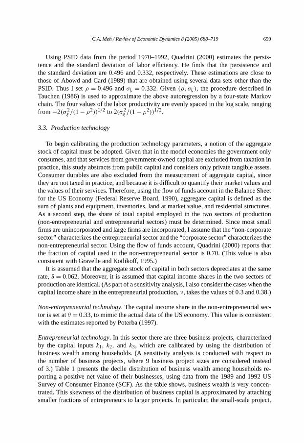
Using PSID data from the period 1970–1992, Quadrini (2000) estimates the ptence and the standard deviation of labor efficiency. He finds that the persistencthe standard deviation are 0.496 and 0.332, respectively. These estimations arethose of Abowd and Card (1989) that are obtained using several data sets other tPSID. Thus I setρ = 0.496 andσξ = 0.332. Given(ρ,σξ ), the procedure describedTauchen (1986) is used to approximate the above autoregression by a four-statechain. The four values of the labor productivity are evenly spaced in the log scale, rafrom −2(σ 2
ξ /(1− ρ2))1/2 to 2(σ 2ξ /(1− ρ2))1/2.
3.3. Production technology
To begin calibrating the production technology parameters, a notion of the aggstock of capital must be adopted. Given that in the model economies the governmeconsumes, and that services from government-owned capital are excluded from taxpractice, this study abstracts from public capital and considers only private tangibleConsumer durables are also excluded from the measurement of aggregate capitathey are not taxed in practice, and because it is difficult to quantify their market valuethe values of their services. Therefore, using the flow of funds account in the Balancefor the US Economy (Federal Reserve Board, 1990), aggregate capital is definedsum of plants and equipment, inventories, land at market value, and residential struAs a second step, the share of total capital employed in the two sectors of prod(non-entrepreneurial and entrepreneurial sectors) must be determined. Since mofirms are unincorporated and large firms are incorporated, I assume that the “non-cosector” characterizes the entrepreneurial sector and the “corporate sector” characternon-entrepreneurial sector. Using the flow of funds account, Quadrini (2000) reporthe fraction of capital used in the non-entrepreneurial sector is 0.70. (This value iconsistent with Gravelle and Kotlikoff, 1995.)
It is assumed that the aggregate stock of capital in both sectors depreciates at thrate,δ = 0.062. Moreover, it is assumed that capital income shares in the two sectproduction are identical. (As part of a sensitivity analysis, I also consider the cases whcapital income share in the entrepreneurial production,ν, takes the values of 0.3 and 0.38.)
Non-entrepreneurial technology. The capital income share in the non-entrepreneurialtor is set atθ = 0.33, to mimic the actual data of the US economy. This value is consiwith the estimates reported by Poterba (1997).
Entrepreneurial technology. In this sector there are three business projects, characteby the capital inputsk1, k2, and k3, which are calibrated by using the distributionbusiness wealth among households. (A sensitivity analysis is conducted with respthe number of business projects, where 9 business project sizes are consideredof 3.) Table 1 presents the decile distribution of business wealth among househoporting a positive net value of their businesses, using data from the 1989 and 19Survey of Consumer Finance (SCF). As the table shows, business wealth is very ctrated. This skewness of the distribution of business capital is approximated by att
smaller fractions of entrepreneurs to larger projects. In particular, the small-scale project,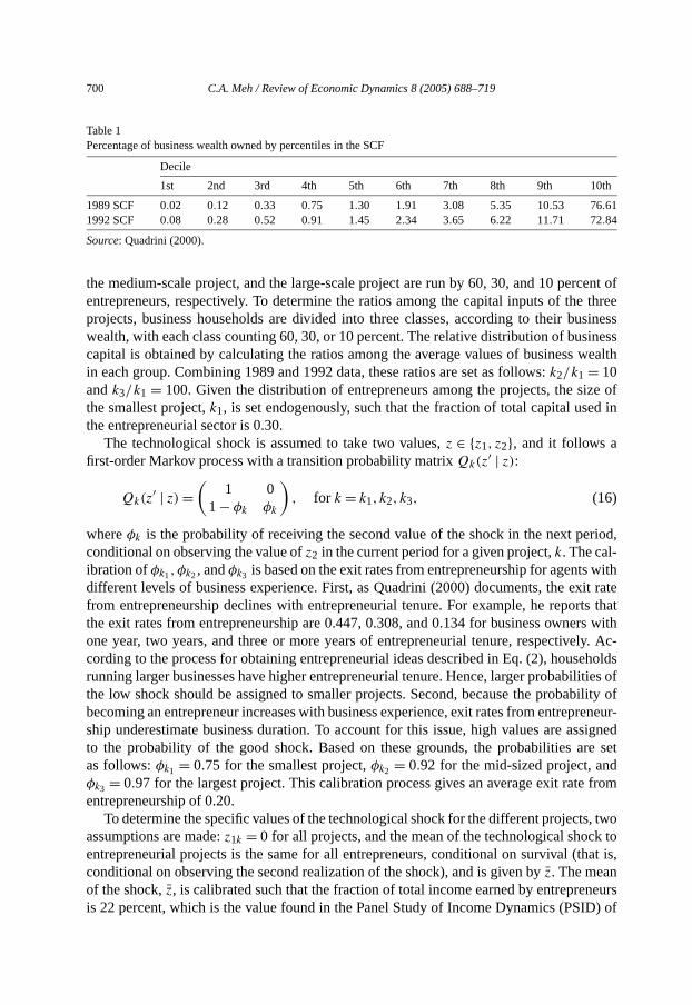
700 C.A. Meh / Review of Economic Dynamics 8 (2005) 688–719
cent ofe threeusinesssinesswealth
ize ofd in
riod,
withxit raterts thatrs withly. Ac-eholdsilities ofbility ofpreneur-ssignedre setdfrom
s, twok tohat is,
neurs
Table 1Percentage of business wealth owned by percentiles in the SCF
Decile
1st 2nd 3rd 4th 5th 6th 7th 8th 9th 10th
1989 SCF 0.02 0.12 0.33 0.75 1.30 1.91 3.08 5.35 10.53 76.611992 SCF 0.08 0.28 0.52 0.91 1.45 2.34 3.65 6.22 11.71 72.84
Source: Quadrini (2000).
the medium-scale project, and the large-scale project are run by 60, 30, and 10 perentrepreneurs, respectively. To determine the ratios among the capital inputs of thprojects, business households are divided into three classes, according to their bwealth, with each class counting 60, 30, or 10 percent. The relative distribution of bucapital is obtained by calculating the ratios among the average values of businessin each group. Combining 1989 and 1992 data, these ratios are set as follows:k2/k1 = 10andk3/k1 = 100. Given the distribution of entrepreneurs among the projects, the sthe smallest project,k1, is set endogenously, such that the fraction of total capital usethe entrepreneurial sector is 0.30.
The technological shock is assumed to take two values,z ∈ {z1, z2}, and it follows afirst-order Markov process with a transition probability matrixQk(z
′ | z):
Qk(z′ | z) =
(1 0
1− φk φk
), for k = k1, k2, k3, (16)
whereφk is the probability of receiving the second value of the shock in the next peconditional on observing the value ofz2 in the current period for a given project,k. The cal-ibration ofφk1, φk2, andφk3 is based on the exit rates from entrepreneurship for agentsdifferent levels of business experience. First, as Quadrini (2000) documents, the efrom entrepreneurship declines with entrepreneurial tenure. For example, he repothe exit rates from entrepreneurship are 0.447, 0.308, and 0.134 for business owneone year, two years, and three or more years of entrepreneurial tenure, respectivecording to the process for obtaining entrepreneurial ideas described in Eq. (2), housrunning larger businesses have higher entrepreneurial tenure. Hence, larger probabthe low shock should be assigned to smaller projects. Second, because the probabecoming an entrepreneur increases with business experience, exit rates from entreship underestimate business duration. To account for this issue, high values are ato the probability of the good shock. Based on these grounds, the probabilities aas follows:φk1 = 0.75 for the smallest project,φk2 = 0.92 for the mid-sized project, anφk3 = 0.97 for the largest project. This calibration process gives an average exit rateentrepreneurship of 0.20.
To determine the specific values of the technological shock for the different projectassumptions are made:z1k = 0 for all projects, and the mean of the technological shocentrepreneurial projects is the same for all entrepreneurs, conditional on survival (tconditional on observing the second realization of the shock), and is given byz. The meanof the shock,z, is calibrated such that the fraction of total income earned by entrepre
is 22 percent, which is the value found in the Panel Study of Income Dynamics (PSID) of
C.A. Meh / Review of Economic Dynamics 8 (2005) 688–719 701
rated:thee tax60, 30,is theta for
-given
ateithrmined
ks,
ratesdiariespercent.
h
1994).1999(1994)
gressions
1970–1992. Givenz and the transition probabilities, the second value of the shock,z2k , isderived from the following equation:
z2k = z
φk
, for k = k1, k2, k3. (17)
The probability distribution,Pk(k), of the entrepreneurial ideak ∈ {0, k1, k2, k3}, is de-fined in Eq. (2). Given this definition, there are only three parameters to be calibP0(k = k1), Pk1(k = k2), and Pk2t (k = k3). They are set endogenously such thatdistribution of entrepreneurs in the stationary equilibrium with a progressive incomsystem equals the imposed distribution of entrepreneurs among the three projects:and 10 percent, respectively. The total fraction of entrepreneurs equals 0.12, whichsame fraction found in the PSID data for the period 1970–1992 and in the SCF da1989–1992.
The calibration of the stochastic depreciation rate,δz, is made under the following assumption: the average depreciation rate for each project, conditional on survival, isby the aggregate depreciation rate,δ. In the benchmark equilibrium, the depreciation rassigned to the bad shock isδz1k
= 0.1 for all projects. (I conduct a sensitivity analysis wrespect to this parameter in Section 6.) The second depreciation value is then deteby the following equation:
δz2k= δ − (1− φk)δz1k
φk
, for all k = k1, k2, k3. (18)
3.4. Intermediation sector
The proportional intermediation cost,γ , charged by intermediaries, particularly banto entrepreneurs, represents the difference between the interest rate on loans,rl , and theinterest rate on deposits,rd . Díaz-Giménez et al. (1992) report the average interestpaid on several types of household borrowing and lending to banks and other intermefor selected years. Based on these data, they calibrate the interest rate spread at 5.5In the benchmark economy, I setrl − rd = γ = 0.055. A sensitivity is conducted witrespect to this parameter.
3.5. Government
In the model economy, the government uses the function,τ (y), to tax individuals’ in-comes to finance its consumption,G. The functional form of the tax function,τ , is basedon the effective household income tax function estimated by Gouevia and Strauss (This tax function is chosen for both its tractability and simplicity (Castañeda et al.,and Sarte, 1997 have also suggested its use). In particular, Gouevia and Strausscharacterize the 1989 US effective personal tax function as follows19:
τ(y) = α0(y − (
y−α1 + α2)−1/α1
), (19)
19 In their study, the authors present a range of parameter estimates obtained from cross-sectional re
involving US individual income and tax data for 1979–1989.
702 C.A. Meh / Review of Economic Dynamics 8 (2005) 688–719
ot unit-es forthat
onomy
inedtion ofhe taxable 2.
ntre-is thechas-in theed byividualsthan
Table 2Calibration of parameters of the model with entrepreneurs
Description Parameters Values
Relative risk aversion σ 2.0Discount factor β 0.934Tax parameters {α0, α1, α2} {0.258,0.768,0.299}Non-entrepreneurial capital income share θ 0.33Entrepreneurial capital income share ν 0.33Depreciation rate of aggregate capital δ 0.062Intermediation cost γ 0.055Entrepreneurial size projects k {0,1.7,17,170}Mean technological shock z 2.374
Values of the shock z2k
3.172.582.45
Probability transition φk
0.750.920.97
Arrival probability of new entrepreneurial ideas Pk(k)
0.0240.1100.075
Stochastic depreciation δz
0.1 0.0490.1 0.0590.1 0.061
with the values of the parametersα0 = 0.258,α1 = 0.768, andα2 = 0.031.However, their estimates cannot be used, because the marginal tax rates are n
free. To solve this problem, I follow Castañeda et al. (1999), by using their estimatα0 andα1, and then calibrateα2 such that the average tax rates paid by a householdearns the mean household income both in the United States and in the artificial ecare identical.
After calibrating the tax function, the value of government consumption is determendogenously by the government budget constraint (7). As a result, the interpretaG in the model economy under the progressive income tax system is the size of tcollection. The parameters’ values for the benchmark economy are summarized in T
3.6. Economy without entrepreneurs
The calibration of the model without entrepreneurs is similar to the model with epreneurs. A key difference regarding the calibration of the two model economiescalibration of labor efficiency. In contrast to the model with entrepreneurs, the stotic process of earnings is now such that the distribution of wealth matches the onemodel with entrepreneurs (and in the US data). To do so, I follow the approach usCastañeda et al. (2003), where the stochastic process of earnings is such that indface a low probability of obtaining a non-persistent productivity shock that is more
1000 times their median income in the economy. They then show that the desire to smooth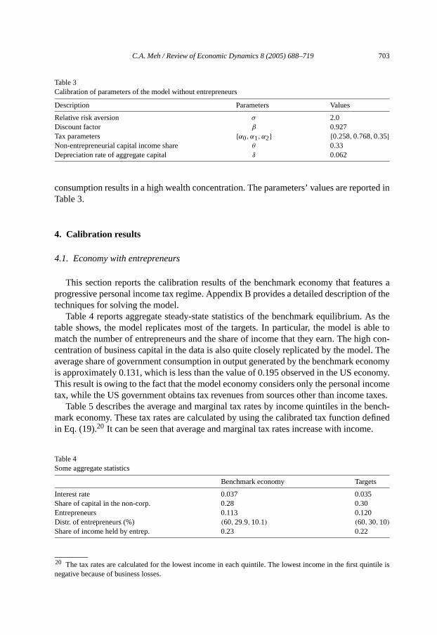
C.A. Meh / Review of Economic Dynamics 8 (2005) 688–719 703
rted in
ures aof the
As theble to
gh con-l. The
conomynomy.cometaxes.
bench-efinede.
intile is
Table 3Calibration of parameters of the model without entrepreneurs
Description Parameters Values
Relative risk aversion σ 2.0Discount factor β 0.927Tax parameters {α0, α1, α2} {0.258,0.768,0.35}Non-entrepreneurial capital income share θ 0.33Depreciation rate of aggregate capital δ 0.062
consumption results in a high wealth concentration. The parameters’ values are repoTable 3.
4. Calibration results
4.1. Economy with entrepreneurs
This section reports the calibration results of the benchmark economy that featprogressive personal income tax regime. Appendix B provides a detailed descriptiontechniques for solving the model.
Table 4 reports aggregate steady-state statistics of the benchmark equilibrium.table shows, the model replicates most of the targets. In particular, the model is amatch the number of entrepreneurs and the share of income that they earn. The hicentration of business capital in the data is also quite closely replicated by the modeaverage share of government consumption in output generated by the benchmark eis approximately 0.131, which is less than the value of 0.195 observed in the US ecoThis result is owing to the fact that the model economy considers only the personal intax, while the US government obtains tax revenues from sources other than income
Table 5 describes the average and marginal tax rates by income quintiles in themark economy. These tax rates are calculated by using the calibrated tax function din Eq. (19).20 It can be seen that average and marginal tax rates increase with incom
Table 4Some aggregate statistics
Benchmark economy Targets
Interest rate 0.037 0.035Share of capital in the non-corp. 0.28 0.30Entrepreneurs 0.113 0.120Distr. of entrepreneurs (%) (60,29.9,10.1) (60,30,10)Share of income held by entrep. 0.23 0.22
20 The tax rates are calculated for the lowest income in each quintile. The lowest income in the first qu
negative because of business losses.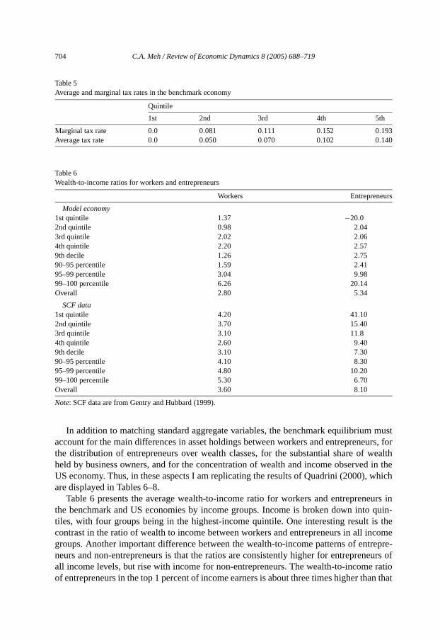
704 C.A. Meh / Review of Economic Dynamics 8 (2005) 688–719
s
musturs, forwealthin the
which
eurs inquin-
is thecome
trepre-eurs ofratio
Table 5Average and marginal tax rates in the benchmark economy
Quintile
1st 2nd 3rd 4th 5th
Marginal tax rate 0.0 0.081 0.111 0.152 0.193Average tax rate 0.0 0.050 0.070 0.102 0.140
Table 6Wealth-to-income ratios for workers and entrepreneurs
Workers Entrepreneur
Model economy1st quintile 1.37 −20.02nd quintile 0.98 2.043rd quintile 2.02 2.064th quintile 2.20 2.579th decile 1.26 2.7590–95 percentile 1.59 2.4195–99 percentile 3.04 9.9899–100 percentile 6.26 20.14Overall 2.80 5.34
SCF data1st quintile 4.20 41.102nd quintile 3.70 15.403rd quintile 3.10 11.84th quintile 2.60 9.409th decile 3.10 7.3090–95 percentile 4.10 8.3095–99 percentile 4.80 10.2099–100 percentile 5.30 6.70Overall 3.60 8.10
Note: SCF data are from Gentry and Hubbard (1999).
In addition to matching standard aggregate variables, the benchmark equilibriumaccount for the main differences in asset holdings between workers and entreprenethe distribution of entrepreneurs over wealth classes, for the substantial share ofheld by business owners, and for the concentration of wealth and income observedUS economy. Thus, in these aspects I am replicating the results of Quadrini (2000),are displayed in Tables 6–8.
Table 6 presents the average wealth-to-income ratio for workers and entreprenthe benchmark and US economies by income groups. Income is broken down intotiles, with four groups being in the highest-income quintile. One interesting resultcontrast in the ratio of wealth to income between workers and entrepreneurs in all ingroups. Another important difference between the wealth-to-income patterns of enneurs and non-entrepreneurs is that the ratios are consistently higher for entreprenall income levels, but rise with income for non-entrepreneurs. The wealth-to-income
of entrepreneurs in the top 1 percent of income earners is about three times higher than that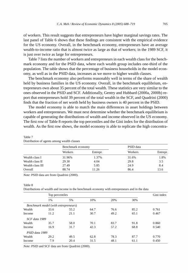
C.A. Meh / Review of Economic Dynamics 8 (2005) 688–719 705
tes. TheidenceverageCF, it
bench-of the
el econ-
wealth, en-
r to the0b) re-(2000).tweenrium isnomy.on ofentra-
r.
of workers. This result suggests that entrepreneurs have higher marginal savings ralast panel of Table 6 shows that these findings are consistent with the empirical evfor the US economy. Overall, in the benchmark economy, entrepreneurs have an awealth-to-income ratio that is almost twice as large as that of workers; in the 1989 Sis just over twice as large for entrepreneurs.
Table 7 lists the number of workers and entrepreneurs in each wealth class for themark economy and for the PSID data, where each wealth group includes one-thirdpopulation. The table shows that the percentage of business households in the modomy, as well as in the PSID data, increases as we move to higher wealth classes.
The benchmark economy also performs reasonably well in terms of the share ofheld by business families in the US economy. Overall, in the benchmark equilibriumtrepreneurs own about 35 percent of the total wealth. These statistics are very similaones observed in the PSID and SCF. Additionally, Gentry and Hubbard (2000a, 200port that entrepreneurs hold 39 percent of the total wealth in the SCF, and Quadrinifinds that the fraction of net worth held by business owners is 40 percent in the PSID
The model economy is able to match the main differences in asset holdings beworkers and entrepreneurs. We must next determine whether the benchmark equilibcapable of generating the distributions of wealth and income observed in the US ecoThe first row of Table 8 reports the top percentiles and the Gini index for the distributiwealth. As the first row shows, the model economy is able to replicate the high conc
Table 7Distribution of agents among wealth classes
Benchmark economy PSID data
Workers Entrepr. Workers Entrep
Wealth class I 31.96% 1.37% 31.6% 1.8%Wealth class II 29.30 4.04 29.8 3.5Wealth class III 27.49 5.85 24.9 8.4Overall 88.74 11.26 86.4 13.6
Note: PSID data are from Quadrini (2000).
Table 8Distributions of wealth and income in the benchmark economy with entrepreneurs and in the data
Top percentiles Gini index
1% 5% 10% 20% 30%
Benchmark model (with entrepreneurs)Wealth 33.6 55.2 64.7 76.6 85.2 0.761Income 11.2 21.1 30.7 49.2 65.1 0.467
SCF data 1989Wealth 35.7 58.0 70.1 83.7 91.8 0.860Income 16.9 31.7 42.3 57.2 68.8 0.540
PSID data 1989Wealth 29.2 49.5 62.8 78.3 87.7 0.770Income 7.9 20.4 31.5 48.1 61.1 0.450
Note: PSID and SCF data are from Quadrini (2000).
706 C.A. Meh / Review of Economic Dynamics 8 (2005) 688–719
alth is1989
ly, 33.6ent ofen thercent ofstribu-to the
ini ofess 11.2cessfulnd the
odeldata.
e it tox sys-rnment
s with
ome. Givenase inncomencome
Table 9Distribution of wealth in the benchmark model without entrepreneurs and in the data
Top percentiles Gini index
1% 5% 10% 20% 30%
No entrepreneurs 33.1 55.8 64.7 76.6 85.3 0.767US data 29.2 49.5 62.8 78.3 87.7 0.770
Note: PSID data are from Quadrini (2000).
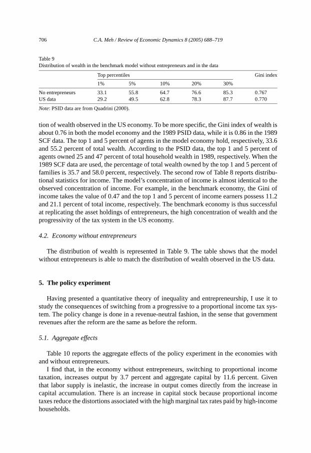
tion of wealth observed in the US economy. To be more specific, the Gini index of weabout 0.76 in both the model economy and the 1989 PSID data, while it is 0.86 in theSCF data. The top 1 and 5 percent of agents in the model economy hold, respectiveand 55.2 percent of total wealth. According to the PSID data, the top 1 and 5 percagents owned 25 and 47 percent of total household wealth in 1989, respectively. Wh1989 SCF data are used, the percentage of total wealth owned by the top 1 and 5 pefamilies is 35.7 and 58.0 percent, respectively. The second row of Table 8 reports ditional statistics for income. The model’s concentration of income is almost identicalobserved concentration of income. For example, in the benchmark economy, the Gincome takes the value of 0.47 and the top 1 and 5 percent of income earners possand 21.1 percent of total income, respectively. The benchmark economy is thus sucat replicating the asset holdings of entrepreneurs, the high concentration of wealth aprogressivity of the tax system in the US economy.
4.2. Economy without entrepreneurs
The distribution of wealth is represented in Table 9. The table shows that the mwithout entrepreneurs is able to match the distribution of wealth observed in the US
5. The policy experiment
Having presented a quantitative theory of inequality and entrepreneurship, I usstudy the consequences of switching from a progressive to a proportional income tatem. The policy change is done in a revenue-neutral fashion, in the sense that goverevenues after the reform are the same as before the reform.
5.1. Aggregate effects
Table 10 reports the aggregate effects of the policy experiment in the economieand without entrepreneurs.
I find that, in the economy without entrepreneurs, switching to proportional inctaxation, increases output by 3.7 percent and aggregate capital by 11.6 percentthat labor supply is inelastic, the increase in output comes directly from the increcapital accumulation. There is an increase in capital stock because proportional itaxes reduce the distortions associated with the high marginal tax rates paid by high-i
households.
C.A. Meh / Review of Economic Dynamics 8 (2005) 688–719 707
rs
aggre-crease
fter thepre-s theirheir in-ts. Mostow run-reneursfactor
nd theneurial
laborneurialore pre-e wageal stockcrease
mongte into
inal taxrsonal
centagestments
d in
Table 10Aggregate effects of the policy experiment in the models with and without entrepreneurs
With entrepreneurs No entrepreneu
(Change) (Change)
Output 5.5% 3.7%Capital stock 6.1% 11.6%Capital input per entrepreneur 16.5% –Labor input per entrepreneur 7.0% –Interest rate −16.2% −19.0%Wage rate 4.1% 3.7%Average marginal tax rate −6.90% −7.01%Average tax rate −2.00% −2.02%
In the economy with entrepreneurs, proportional income tax reform increasesgate output by 5.5 percent. This result is mainly caused by both the 17 percent inin entrepreneurial investments and the 6 percent increase in aggregate capital.21 Thereis an increase in the capital stock in the economy with entrepreneurs because atax reform, the marginal tax rate on rich individuals falls. Given that existing entreneurs are mostly high-income individuals, they increase their savings and this relaxeborrowing constraints. As a result of these higher savings, entrepreneurs increase tvestments, and hence expand their businesses by running larger and better projecentrepreneurs running small and medium-sized businesses before the reform are nning larger scale businesses. Consequently, there is a better allocation of entrepover project sizes. As explained in the next section, this can lead to a rise in totalproductivity (TFP) which, in turn, augments output (see also Erosa, 2001).
When entrepreneurship is modelled explicitly, both the aggregate capital stock acapital input in the entrepreneurial production sector increase, as does non-entreprecapital.22 This rise in non-entrepreneurial capital, coupled with the high demand forinput in the entrepreneurial sector, raises the capital–labor ratio in the non-entrepresector, which, in turn, decreases the interest rate and increases the wage rate. Mcisely, as indicated in Table 10, the interest rate drops by about 16 percent and thrate rises by 4 percent. In the model without entrepreneurs, the increase in the capitdirectly translates into a rise in the aggregate capital–labor ratio, and therefore, a dein the interest rate by 19 percent and an increase in the wage rate by 3.7 percent.
Table 11 reports the fraction of entrepreneurs, the distribution of entrepreneurs abusiness projects (also called the distribution of business wealth), and the entry ra
21 The increase in business investment after the elimination of progressive taxation that cuts the margrate paid by entrepreneurs is in line with the finding of Carroll et al. (1998a), who estimate that high peincome taxes significantly affect the investment decisions of small firms. To be specific, they find that a perpoint increase in marginal tax rates reduces the proportion of entrepreneurs who make new capital inveby 10.4 percent, and decreases mean investment expenditures by 9.9 percent.22 Recall that the market-clearing conditions are given byKc = K − Kn andNc = N − Nn, for capital andlabor markets, respectively. The variablesKn andNn denote the aggregation of capital and labor inputs use
the entrepreneurial sector, respectively.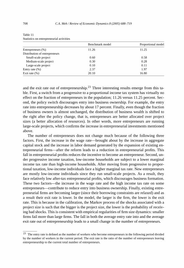
708 C.A. Meh / Review of Economic Dynamics 8 (2005) 688–719
el
ta-lly not. Sec-entry
fractionifted toprojectunningntioned
threegregateting en-. Thisnd, un-
arginalopor-neurs, theyation.some
entre-and asexitwith a
eceiv-aller
erageeurs.
dividedleaving
Table 11Statistics on entrepreneurial activities
Benchmark model Proportional mod
Entrepreneurs (%) 11.26 11.25Distribution of entrepreneurs
Small-scale project 0.60 0.58Medium-scale project 0.30 0.28Large-scale project 0.10 0.11
Entry rate (%) 2.37 1.97Exit rate (%) 20.10 16.80
and the exit rate out of entrepreneurship.23 Three interesting results emerge from thisble. First, a switch from a progressive to a proportional income tax system has virtuaeffect on the fraction of entrepreneurs in the population; 11.26 versus 11.25 percenond, the policy switch discourages entry into business ownership. For example, therate into entrepreneurship decreases by about 17 percent. Finally, even though theof business owners is almost unchanged, the distribution of business wealth is shthe right after the policy change, that is, entrepreneurs are better allocated oversizes (a better allocation of resources). In other words, more entrepreneurs are rlarge-scale projects, which confirms the increase in entrepreneurial investments meabove.
The number of entrepreneurs does not change much because of the followingfactors. First, the increase in the wage rate—brought about by the increase in agcapital stock and the increase in labor demand generated by the expansion of existrepreneurial firms—after the reform leads to a reduction in entrepreneurial profitsfall in entrepreneurial profits reduces the incentive to become an entrepreneur. Secoder progressive income taxation, low-income households are subject to a lower mincome tax rate than high-income households. After moving from progressive to prtional taxation, low-income individuals face a higher marginal tax rate. New entrepreare mostly low-income individuals since they run small-scale projects. As a resultface relatively low after-tax entrepreneurial profits, which discourages business formThese two factors—the increase in the wage rate and the high income tax rate onentrepreneurs—contribute to reduce entry into business ownership. Finally, existingpreneurial firms are becoming larger (since their borrowing constraints are relaxed)a result their exit rate is lower. In the model, the larger is the firm, the lower is therate. This is because in the calibration, the Markov process of the shocks associatedproject size is such that the bigger is the project size, the lower is the probability of ring bad shocks. This is consistent with empirical regularities of firm size dynamics: smfirms fail more than large firms. The fall in both the average entry rate into and the avexit rate out of entrepreneurship leads to a small change in the number of entrepren
23 The entry rate is defined as the number of workers who become entrepreneurs in the following periodby the number of workers in the current period. The exit rate is the ratio of the number of entrepreneurs
entrepreneurship to the current total number of entrepreneurs.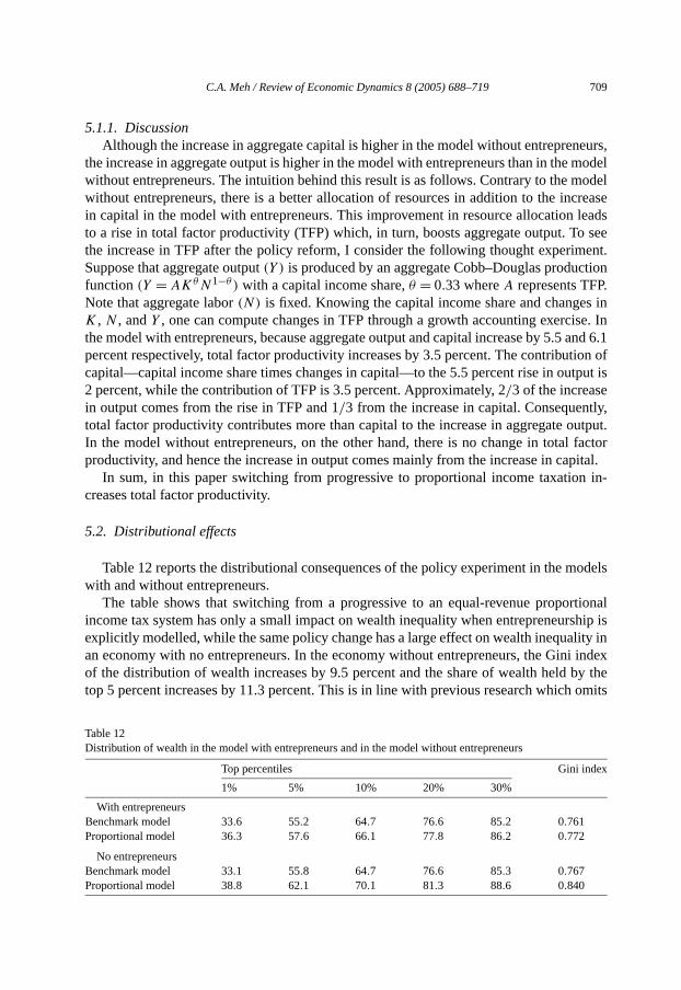
C.A. Meh / Review of Economic Dynamics 8 (2005) 688–719 709
neurs,modelodel
creaseleads
o seeent.
tion.s inise. Inand 6.1
tion oftput is
tly,utput.factor
pital.n in-
odels
rtionalship islity ini indexby theomits
5.1.1. DiscussionAlthough the increase in aggregate capital is higher in the model without entrepre
the increase in aggregate output is higher in the model with entrepreneurs than in thewithout entrepreneurs. The intuition behind this result is as follows. Contrary to the mwithout entrepreneurs, there is a better allocation of resources in addition to the inin capital in the model with entrepreneurs. This improvement in resource allocationto a rise in total factor productivity (TFP) which, in turn, boosts aggregate output. Tthe increase in TFP after the policy reform, I consider the following thought experimSuppose that aggregate output(Y ) is produced by an aggregate Cobb–Douglas producfunction(Y = AKθN1−θ ) with a capital income share,θ = 0.33 whereA represents TFPNote that aggregate labor(N) is fixed. Knowing the capital income share and changeK , N , andY , one can compute changes in TFP through a growth accounting exercthe model with entrepreneurs, because aggregate output and capital increase by 5.5percent respectively, total factor productivity increases by 3.5 percent. The contribucapital—capital income share times changes in capital—to the 5.5 percent rise in ou2 percent, while the contribution of TFP is 3.5 percent. Approximately, 2/3 of the increasein output comes from the rise in TFP and 1/3 from the increase in capital. Consequentotal factor productivity contributes more than capital to the increase in aggregate oIn the model without entrepreneurs, on the other hand, there is no change in totalproductivity, and hence the increase in output comes mainly from the increase in ca
In sum, in this paper switching from progressive to proportional income taxatiocreases total factor productivity.
5.2. Distributional effects
Table 12 reports the distributional consequences of the policy experiment in the mwith and without entrepreneurs.
The table shows that switching from a progressive to an equal-revenue propoincome tax system has only a small impact on wealth inequality when entrepreneurexplicitly modelled, while the same policy change has a large effect on wealth inequaan economy with no entrepreneurs. In the economy without entrepreneurs, the Ginof the distribution of wealth increases by 9.5 percent and the share of wealth heldtop 5 percent increases by 11.3 percent. This is in line with previous research which
Table 12Distribution of wealth in the model with entrepreneurs and in the model without entrepreneurs
Top percentiles Gini index
1% 5% 10% 20% 30%
With entrepreneursBenchmark model 33.6 55.2 64.7 76.6 85.2 0.761Proportional model 36.3 57.6 66.1 77.8 86.2 0.772
No entrepreneursBenchmark model 33.1 55.8 64.7 76.6 85.3 0.767Proportional model 38.8 62.1 70.1 81.3 88.6 0.840
710 C.A. Meh / Review of Economic Dynamics 8 (2005) 688–719
rtionalindex,nd thectively.
llows:hingcreases facedave lessnflict-houtdiffer-effect.te ben-urs,
l profitsducese. Their sav-roup ofentre-ithouturs in-
ivity ofmber
uction,ck.
restric-More
e these
th
entrepreneurship. For example, Castañeda et al. (1999) find that a switch to propoincome taxation substantially increases wealth inequality, as measured by the Giniby 10.5 percent. By contrast, in the model with entrepreneurs, the wealth Gini index ashare of wealth held by the top 5 percent increase by only 1.4 and 4.3 percent, respe
5.2.1. DiscussionThe intuition behind the result in the previous section can be summarized as fo
in the model with only workers, the large increase in wealth inequality when switcfrom a progressive to a proportional income tax system is mainly caused by the dein marginal tax rates paid by rich households and the increase in marginal tax rateby low-income households. Wealthy households save more and poor households sleading to higher wealth inequality. In the model with entrepreneurs, there are two coing effects on wealth inequality. In addition to the impact found in the economy witentrepreneurs, there is an offsetting effect that reduces wealth inequality. The mainence in the effects on wealth inequality between the two economies is in the wageMore specifically, in the economy without entrepreneurs, the increase in the wage raefits all individuals (low or high-income individuals). In the economy with entrepreneon the other hand, the increase in the wage rate tends to reduce entrepreneuriawhile it increases the wage income of workers. The fall in entrepreneurial profits rethe incentive of existing entrepreneurs—who are mostly richer—to invest and to savincrease in the wage income of workers—who are most likely to be poor—raise theings. As a result, the rise in the wage rate decreases wealth inequality between the gworkers and entrepreneurs. This effect, which is only present in the economy withpreneurs, partially offsets the increase in wealth inequality observed in the model wentrepreneurs so that the overall wealth inequality in the economy with entreprenecreases only slightly.
6. Sensitivity analysis
This section presents some computational experiments to determine the sensitthe numerical findings of the previous section: a version of the model with a higher nuof business size, a higher and a lower elasticity of capital in the entrepreneurial prodand the borrowing constraints and the stochastic properties of the technological sho
6.1. Increasing the number of business projects
The specification of the set of business size as a set of three elements may seemtive. In this section I report the results for specifications with more business sizes.specifically, I consider 9 business project sizes in three clusters of three. Let’s denotclusters by cluster 1, cluster 2 and cluster 3. Given the initial three project sizes—k1, k2,andk3—in the original model, a clusteri (for i = 1,2,3) consists of three elements wi
an average business size ofki where the first element is�i percent less thanki , the second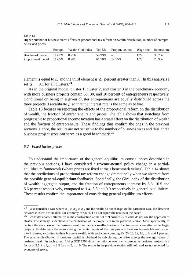
C.A. Meh / Review of Economic Dynamics 8 (2005) 688–719 711
trepre-
t rate
nomyctively.ss the
utionfrom
ealtheviousus, three
ibed inpartial-hows
t fromution.5 andbrium.
nces
roach ofally, to
d to largere dividedpercent.
alues ofjects is ad for
Table 13Higher number of business sizes: effects of proportional tax reform on wealth distribution, number of enneurs, and prices
Entrepr. Wealth Gini index Top 5% Proport. tax rate Wage rate Interes
Benchmark model 11.67% 0.776 59.99% – 1.22 3.52%Proportional model 11.65% 0.781 61.70% 14.75% 1.28 2.69%
element is equal toki and the third element is�i percent greater thanki . In this analysis Iset�i = 0.1 for all clusters.24
As in the original model, cluster 1, cluster 2, and cluster 3 in the benchmark ecowith more business projects contain 60, 30, and 10 percent of entrepreneurs respeConditional on being in a given cluster entrepreneurs are equally distributed acrothree projects. I recalibrateβ so that the interest rate is the same as before.
Table 13 focuses on reporting the effects of the proportional reform on the distribof wealth, the fraction of entrepreneurs and prices. The table shows that switchingprogressive to proportional income taxation has a small effect on the distribution of wand the fraction of entrepreneurs. These findings thus confirm the ones in the prsections. Hence, the results are not sensitive to the number of business sizes and thbusiness project sizes can serve as a good benchmark.25
6.2. Fixed factor prices
To understand the importance of the general-equilibrium consequences descrthe previous sections, I have considered a revenue-neutral policy change in aequilibrium framework (where prices are fixed at their benchmark values). Table 14 sthat the predictions of proportional tax reform change dramatically when we abstracthe possible general-equilibrium feedbacks. Specifically, the Gini index of the distribof wealth, aggregate output, and the fraction of entrepreneurs increase by 5.3, 166.6 percent respectively, compared to 1.4, 5.5 and 0.0 respectively in general equiliThese results confirm the importance of considering general equilibrium effects.
24 I also consider a case where�1 �= �2 �= �3 and the results do not change. In this particular case, the distabetween clusters are smaller. For economy of space, I do not report the results in the paper.25 I consider another alternative in the construction of the set of 9 business sizes that do not use the appcluster. The strategy is identical to the calibration of the project size in the previous section. More specificcapture the skewness of the business wealth in the data smaller fractions of entrepreneurs are attacheprojects. To determine the ratios among the capital inputs of the nine projects, business households arinto 9 classes, according to their business wealth, with each class counting 25, 20, 15, 12, 10, 8, 6, and 1The relative distribution of business capital is obtained by calculating the ratios among the average vbusiness wealth in each group. Using SCF 1998 data, the ratio between two consecutive business profactor of 2.5:ki/ki−1 = 2.5 for i = 2, . . . ,9. The results in the previous section still hold and are not reporte
economy of space.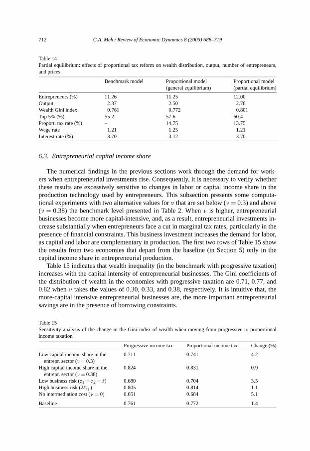
712 C.A. Meh / Review of Economic Dynamics 8 (2005) 688–719
neurs,
el)
ork-hether
e in themputa-
lents in-
y in theor labor,show
in the
ation)nts of, and
t, theneurial
rtional
(%)
Table 14Partial equilibrium: effects of proportional tax reform on wealth distribution, output, number of entrepreand prices
Benchmark model Proportional model Proportional mod(general equilibrium) (partial equilibrium
Entrepreneurs (%) 11.26 11.25 12.00Output 2.37 2.50 2.76Wealth Gini index 0.761 0.772 0.801Top 5% (%) 55.2 57.6 60.4Proport. tax rate (%) – 14.75 13.75Wage rate 1.21 1.25 1.21Interest rate (%) 3.70 3.12 3.70
6.3. Entrepreneurial capital income share
The numerical findings in the previous sections work through the demand for wers when entrepreneurial investments rise. Consequently, it is necessary to verify wthese results are excessively sensitive to changes in labor or capital income sharproduction technology used by entrepreneurs. This subsection presents some cotional experiments with two alternative values forν that are set below (ν = 0.3) and above(ν = 0.38) the benchmark level presented in Table 2. Whenν is higher, entrepreneuriabusinesses become more capital-intensive, and, as a result, entrepreneurial investmcrease substantially when entrepreneurs face a cut in marginal tax rates, particularlpresence of financial constraints. This business investment increases the demand fas capital and labor are complementary in production. The first two rows of Table 15the results from two economies that depart from the baseline (in Section 5) onlycapital income share in entrepreneurial production.
Table 15 indicates that wealth inequality (in the benchmark with progressive taxincreases with the capital intensity of entrepreneurial businesses. The Gini coefficiethe distribution of wealth in the economies with progressive taxation are 0.71, 0.770.82 whenν takes the values of 0.30, 0.33, and 0.38, respectively. It is intuitive thamore-capital intensive entrepreneurial businesses are, the more important entrepresavings are in the presence of borrowing constraints.
Table 15Sensitivity analysis of the change in the Gini index of wealth when moving from progressive to propoincome taxation
Progressive income tax Proportional income tax Change
Low capital income share in theentrepr. sector (ν = 0.3)
0.711 0.741 4.2
High capital income share in theentrepr. sector (ν = 0.38)
0.824 0.831 0.9
Low business risk (z1 = z2 = z) 0.680 0.704 3.5High business risk (2δz1) 0.805 0.814 1.1No intermediation cost (γ = 0) 0.651 0.684 5.1
Baseline 0.761 0.772 1.4
C.A. Meh / Review of Economic Dynamics 8 (2005) 688–719 713
er the
tech-ges in
busi-erefore
fourthres-m theidio-
ation ofs that
gres-of the
htnesse taxg con-ectionse theg the
act ofof thewing
reasessevere.eurs’ake thecapitalin an
eurs andorkers
theirsults in
Further, the table reveals that the size of the increase in wealth inequality aftelimination of progressive taxation is negatively related toν. More specifically, the policyswitch increases the wealth Gini index by 4.2, 1.4, and 0.9 percent whenν takes the valueof 0.30, 0.33, and 0.38, respectively. This is due to the fact that as the productionnology becomes less (more) capital intensive, the effects on wages driven by chanentrepreneurial savings behavior become less (more) important.
6.4. Borrowing constraints and business risk
The borrowing limits (the minimum of assets necessary to start or to expand aness) are determined by the stochastic properties of the technological shocks. Ththe sensitivity analysis with respect to this parameter provides ajoint evaluation of theimportance of the riskiness of the business and the borrowing limits. The third androws of Table 15 display the Gini coefficient of the distribution of wealth for both progsive and proportional income taxes and the change in this coefficient that results fropolicy reform when business risk is high and low. Low business risk arises when thesyncratic technological shock takes the mean value, that isz1 = z2 = z, while high businessrisk corresponds to a case where the depreciation rate associated with a low realizthe shock is being doubled. In the current context low (high) business risk implieborrowing limits are less (more) binding.
As the table indicates, wealth inequality in the benchmark economies (with prosive income tax system) is quite sensitive to changes in the stochastic propertiestechnological shock. For example, when the riskiness of business is high (or the tigof borrowing constraints is severe) the Gini coefficient of wealth in the progressivsteady state increases from 0.76 to 0.81. When business risk is low (or borrowinstraints are less tight) the Gini index of wealth decreases from 0.76 to 0.68. The dirof the change is natural since high business risk and tighter borrowing limits increaincentive of individuals to save more for precautionary motives and for overcominborrowing constraints (see Quadrini, 2000).
Interestingly, as can be seen from the third and fourth rows of the table the impa switch from progressive to proportional income taxation depends on the riskinessbusiness activity and the tightness of borrowing limits. For example, when the borroconstraints are binding and business risks are high the Gini coefficient of wealth incby only 1.1 percent, while it increases by 3.5 percent when these constraints are lessThis is intuitive because when the borrowing limits are binding, the cut in entreprenmarginal tax rate relaxes the borrowing constraints and entrepreneurs are able to mdiscrete investments that are required. Because of the complementarity of labor andin entrepreneurial production function, the demand for labor increases which resultsincrease in the wage rate. This increase in the wage rate reduces profits of entreprenincrease earnings of workers. This mechanism narrows wealth inequality between wand entrepreneurs.
When borrowing constraint faced by entrepreneurs are less binding, the cut inmarginal tax rate leads to a modest increase in entrepreneurial investments. This re
a modest increase in the wage rate given the complementarity of labor and capital.
714 C.A. Meh / Review of Economic Dynamics 8 (2005) 688–719
is the-ffectszeroeasesreasediationced by
re re-uality
tivelyts andects ofraints-Eakin
regatestem.
ations,effectct ofitch.witch
s downws theto a re-cialto pro-operateapital
comes. Theentre-
e tax-usiness
6.5. No intermediation costs
Another important parameter that explains the high saving rate of entrepreneursintermediation cost,γ . The fifth row displays the results whenγ = 0. As expected, decreasingγ from 0.055 to 0.0 decreases the wealth Gini index from 0.76 to 0.65. The eon wealth inequality of the policy reform also hinge on the intermediation cost. Withintermediation costs, a shift from progressive to proportional income taxation incrthe Gini coefficient of the distribution of wealth by 5.1 percent, compared to the incof 1.4 percent in the benchmark experiment. This is natural because when intermecosts are zero the change in capital investment that results from a cut tax rates faentrepreneurs is relatively small.
It is worth pointing out that when financial constraints faced by entrepreneurs alaxed or when there is costless financial intermediation the increase in wealth ineqthat results from the switch from progressive to proportional income taxation is relalarge. This suggests that a model of entrepreneurship in which financial constrainbusiness risks are severe is crucial to explain the distributional and aggregate effeliminating progressive taxation. Many empirical studies show that financial constplay an important role in business creation (see Evans and Jovanovic, 1989; Holaltzet al. 1994a, 1994b; Quadrini, 1999; and Gentry and Hubbard, 1999).
7. Conclusion
This paper has shown that entrepreneurship is important in quantifying the aggand distributional effects of reducing the degree of progressivity in the income tax syContrary to previous literature, I find that under a reasonable parameter configurswitching from a progressive to a proportional income tax system has a negligibleon wealth inequality. This surprising result is accounted for by the moderating effeentrepreneurial activities on changes in wealth distribution arising from the policy swMore precisely, an increase in entrepreneurial investments implied by the policy sinduces a higher demand for labor, which raises the wage rate of workers and drivethe average return to business ownership. This general-equilibrium feedback narroincome and savings gap between workers and entrepreneurs, and, in turn, leadsduction in income and wealth inequality. A crucial factor driving this result is financonstraints faced by entrepreneurs. A cut in the tax rate brought about by the switchportional taxation relaxes the financial constraints of entrepreneurs and are able totheir business with higher capital investment and therefore higher labor given that cand labor are complements in the production.
The framework used is an occupational choice model, in which the decision to bean entrepreneur is determined by the ability to manage a firm and by asset holdingmodel also accounts for the high concentration of wealth and the high saving rate ofpreneurs observed in the data.
An interesting extension of this model would be to study the effects of progressivation in an economy characterized by endogenous tax deductions (e.g., excessive b
expenses). This avenue of research is promising, as it has long been argued that entre-
C.A. Meh / Review of Economic Dynamics 8 (2005) 688–719 715
andnothereurs inuan-neurialank-of the
tensions
d JimLuisa, Vin-at thetheinancereferee. All
theis-
theision
h as pro-ntracts.
preneurs or self-employed individuals have more flexibility in making deductionsreclassifying their income (e.g., Barro and Sahasakul, 1983 and Gordon, 1997). Aimportant extension is to endogenize the borrowing constraint faced by entreprenan environment of limited contract enforceability. By doing so it is possible to study qtitatively the insurance aspect of progressive taxation in the presence of entrepreactivity.26 Finally, given the high risk in entrepreneurship and the fact that personal bruptcy provides partial insurance, an important research agenda is the investigationconsequences of personal bankruptcy on entrepreneurship and welfare. These exare left for future research.
Acknowledgments
I am grateful to both my co-supervisors Andrés Erosa and Gustavo Ventura anDavies for continuous advice and comments. I wish also to thank Audra Bowlus,Fuster, Scott Hendry, Ig Horstmann, Kevin Moran, Steve Pischke, Shannon Seitzcenzo Quadrini, Yaz Terajima, Greg Tkacz, John Whalley, and seminar participantsUniversity of Western Ontario, HEC-University of Montreal, Concordia University,Bank of Canada, the Federal Reserve Bank of Cleveland and the Department of Fof Canada for their helpful suggestions. I also thank the associate editor and thefor their insightful comments. I also benefited from a discussion with Randy Wrighterrors are mine.
Appendix A. Definition of a stationary equilibrium
A stationary recursive equilibrium is a pair of value functions,υ(ε, a, k, z) andυ(ε, a, k, z, k, ε′); decision rules,{n(k, z), ga(ε, a, k, z, k, ε′), gk(ε, a, k, z, k, ε′)}; a gov-ernment policy,{G, τ(y)}; prices,{ω, rd, rl}; aggregate capital and labor demands incorporate sector,{Kc,Nc}; and a function,Ψ (µ), that maps the space of households’ dtribution,µ, into the next period distribution, such that:
(1) The decision rules,ga(·) andgk(·), solve the agent’s problem described in (13), andfunctions,υ(·) andυ(·), are the associated value functions, the employment decfor an entrepreneur solves his profit maximization (8).
(2) Prices are competitive; that is,
ω = (1− θ)
(Kc
Nc
)θ
, (A.1)
rd = θ
(Kc
Nc
)θ−1
− δ, (A.2)
26 Krueger and Perri (1999) have started investigating the consequences of redistributive taxation, sucgressive taxation, in an endogenous incomplete market that stems from limited enforceability of private co
However, they do not consider how the insurance aspect of progressive taxation affects entrepreneurial risk-taking.
716 C.A. Meh / Review of Economic Dynamics 8 (2005) 688–719
s
of thensistent
e-
mea-
ulting
rl = rd + γ. (A.3)
(3) The government budget constraint is satisfied; that is,
G =∑ε,k,z
{∫a
τ(y(ε, a, k, z)
)µ(ε, a, k, z)da
}. (A.4)
(4) Capital and labor markets clear; that is,∑ε,k,z
{∫a
kµ(ε, a, k, z)da
}+ Kc =
∑ε,k,z
{∫a
aµ(ε, a, k, z)da
}, (A.5)
∑ε,k,z
{∫a
n(k, z)µ(ε, a, k, z)da
}+ Nc =
∑ε,k,z
{∫a
εµ(ε, a, k, z)da
}. (A.6)
(5) The distribution of the households,µ, is the fixed point of the law of motion,Ψ . Thislaw of motion is consistent with individual decision rules, and given the subsetSε,Sa , Sk , Sz, is defined by the functional equation
µ′(Sε, Sa, Sk, Sz) = Ψ (Sε, Sa, Sk, Sz)
=∑
k
∑ε′∈Sε
∑k′∈Sk
∑z′∈Sz
{ ∫a′∈Sa
∑ε,k,z
{∫a
I(ε, a, k, z, k, ε′)Pk
(k)Γ (ε′, ε)
× Qk(z′, z)µ(ε, a, k, z)da
}da′
}, (A.7)
whereI (ε, a, k, z, k, ε′) is an indicator function defined by
I(ε, a, k, z, k, ε′) =
{1, if ga(ε, a, k, z, k, ε′) ∈ Sa andgk(ε, a, k, z, k, ε′) ∈ Sk,
0, otherwise.(A.8)
Appendix B. Computation of an equilibrium
This appendix describes the algorithm used to compute the stationary equilibriabenchmark economy. The algorithm also computes the parameter values that are cowith the targets.
(1) Guess seven parameters: the discount factor,β; the mean technology in the entreprneurial sector,z; the tax parameter,α2; the smallest size of business project,k1; andthe probabilitiesP0(k = k1), Pk1(k = k2), andPk2(k = k3).
(2) Solve the household’s problem by iterating on the value functions.(3) Use the decision rules to compute a stationary distribution by iterating on the
sure,µ.(4) Check the following conditions:
(a) the capital-to-labor ratio generated in this equilibrium is equal to the one res
from the calibration of the non-entrepreneurial technology,
C.A. Meh / Review of Economic Dynamics 8 (2005) 688–719 717
e sta-cent,
0.22,in the
eters
Press,
a 57 (2),
09 (3),
ability.
Eco-
n the
Political
urnal of
iew 56
ational
eserve
eserve
t. Work-
. Work-
axation:ity of
Journal
(b) the distribution of entrepreneurs among the four projects, generated in thtionary equilibrium, equals the targeted distribution (7.2, 3.6, and 1.2 perrespectively),
(c) the share of income earned by entrepreneurs in the stationary equilibrium is(d) the tax rates paid by a household that earns the mean household income
stationary equilibrium and in the US economy are equal,(e) the fraction of capital employed in the entrepreneurial sector is 0.30.
If conditions (a), (b), (c), (d), and (e) are all satisfied, then an equilibrium is found.If not, make new guesses of{β, z, α2, k1,P0(k = k1),Pk1(k = k2),Pk2(k = k3)}, and go
to step 2.The code is written in Fortran and uses the routine AMOEBA to solve for the param
(see Press et al., 1994). It can be provided by the author upon request.
References
Aaron, H.J., Gale, W.G., 1996. Economic Effects of Fundamental Tax Reform. Brookings InstitutionsWashington, DC.
Abowd, J.M., Card, D., 1989. On the covariance structure of earnings and hours changes. Econometric411–445.
Aiyagari, S.R., 1994. Uninsured idiosyncratic risk, aggregate saving. Quarterly Journal of Economics 1659–684.
Albuquerque, R., Hopenhyan, H.A., 1997. Optimal dynamic lending contracts with imperfect enforceManuscript. University of Rochester.
Altig, D., Carlstrom, C.T., 1999. Marginal tax rates and income inequality in a life-cycle model. Americannomic Review 89 (5), 1197–1215.
Altig, D., Auerbach, A., Kotlikoff, L., Smetters, K., Wallise, J., 2001. Simulating fundamental tax reform iunited states. American Economic Review 91 (3), 574–575.
Auerbach, A., Kotlikoff, L., 1987. Dynamic Fiscal Policy. Cambridge Univ. Press.Banerjee, A., Newman, A.F., 1993. Occupational choice and the process of development. Journal of
Economy 101 (2), 274–298.Barro, R.J., Sahasakul, C., 1983. Measuring the average marginal tax rate from individual income tax. Jo
Business 123 (7), 3–16.Bednarzik, R.W., 2000. The role of entrepreneurship in US and European job growth. Monthly Labor Rev
(4), 419–452.Boadway, R., Marchand, M., Pestieau, P., 1991. Optimal linear income taxation in models with occup
choice. Journal of Public Economics 46, 133–162.Cagetti, M., De Nardi, M., 2002. Entrepreneurship, frictions, and wealth. Working paper No. 620. Federal R
Bank of Minneapolis.Cagetti, M., De Nardi, M., 2004. Taxation, entrepreneurship, and wealth. Staff report No. 340. Federal R
Bank of Minneapolis.Carroll, R., Holtz-Eakin, D., Rider, M., Rosen, H.S., 1998a. Entrepreneurs, income taxes, and investmen
ing paper No. 6374. NBER.Carroll, R., Holtz-Eakin, D., Rider, M., Rosen, H.S., 1998b. Income taxes and entrepreneurs’ use of labor
ing paper No. 6375. NBER.Castañeda, A., Díaz-Giménez, J., Ríos-Rull, J.V., 1999. Earnings and wealth inequality and income t
Quantifying the trade-offs of switching to a proportional income tax in the US. Manuscript. UniversPennsylvania.
Castañeda, A., Díaz-Giménez, J., Ríos-Rull, J.V., 2003. Accounting for earnings and wealth inequality.
of Political Economy 111 (4), 818–857.
718 C.A. Meh / Review of Economic Dynamics 8 (2005) 688–719
eserve
ilibrium
ynam-
Univer-
674.ts. Jour-
rooking
nomy 1,
iversity., AEA
sity.firms.
netary
pirical
te and
nomic
d.), Are
ic Re-
con-
RAND
–494.ualityl Econ-
o. 262.
l Econ-
rio.61.
national
Quarterly
ientific
De Nardi, M., 2000. Wealth inequality and intergenerational links. Working paper No. 99-13. Federal RBank of Chicago.
Díaz-Giménez, J., Prescott, E.C., Fitzgerald, T., Alvarez, F., 1992. Banking in computable general equeconomies. Journal of Economic Dynamics and Control 16, 533–559.
Erosa, A., 2001. Financial intermediation and occupational choice in development. Review of Economic Dics 4 (2), 303–334.
Erosa, A., Koreshkova, T., 2003. Progressive taxation in a dynastic model of human capital. Manuscript.sity Toronto.
Evans, D.S., 1987. Tests of alternative theories of firm growth. Journal of Political Economy 95 (4), 657–Evans, D.S., Jovanovic, B., 1989. An estimated model of entrepreneurial choice under liquidity constrain
nal of Political Economy 97 (4), 808–827.Fazzari, S.M., Hubbard, R.G., Petersen, B.C., 1988. Financing constraints and corporate investment. B
Papers on Economic Activity 88 (1), 141–195.Federal Reserve Board, 1990. Distribution of tangible asset by sector. Balance Sheet for the US Eco
13–18.Gentry, W.M., Hubbard, R.G., 1999. Entrepreneurship and households saving. Manuscript. Columbia UnGentry, W.M., Hubbard, R.G., 2000a. Tax policy and entrepreneurial entry. American Economic Review
Papers and Proceedings 90 (2), 283–287.Gentry, W.M., Hubbard, R.G., 2000b. Tax policy and entrepreneurial entry. Manuscript. Columbia UniverGertler, M., Gilchrist, S., 1994. Monetary policy, business cycles, and the behavior of small manufacturing
Quarterly Journal of Economics CIX (2), 309–340.Gordon, R.H., 1997. Do tax rates encourage activity? Working paper No. WP/97/88. International Mo
Fund.Gouevia, M., Strauss, R.P., 1994. Effective federal individual income tax functions: An exploratory em
analysis. National Tax Journal 47 (2), 317–339.Gravelle, J., Kotlikoff, L.J., 1989. The incidence and efficiency costs of corporate taxation when corpora
non-corporate firms produce the same good. Journal of Political Economy 97 (4), 749–780.Gravelle, J., Kotlikoff, L.J., 1995. Corporate taxation and the efficiency gains of 1986 Tax Reform Act. Eco
Theory 6 (1), 51–81.Haltiwanger, J., Krizan, C.J., 1999. Small business and job creation in the United States. In: Acs, Z.J. (E
Small Firms Important? Massachusetts Academic Publisher.Heckman, J.J., Lochner, L., Taber, C., 1998. Tax policy and human capital formation. American Econom
view, AEA Papers and Proceedings 88 (2), 293–297.Holtz-Eakin, D., Joulfaian, D., Rosen, H.S., 1994a. Sticking it out: Entrepreneurial survival and liquidity
straints. Journal of Political Economy 102 (1), 53–75.Holtz-Eakin, D., Joulfaian, D., Rosen, H.S., 1994b. Entrepreneurial decisions and liquidity constraints.
Journal of Economics 25 (2), 334–347.Huggett, M., 1996. Wealth distribution in life-cycle economies. Journal of Monetary Economics 38 (3), 469Kanbur, S.M.R., 1982. Entrepreneurial risk taking, inequality and public policy: An application of ineq
decomposition analysis to the general equilibrium effects of progressive taxation. Journal of Politicaomy 90 (1), 1–21.
Krueger, D., Perri, F., 1999. Risk sharing: Private insurance markets or redistributive taxes? Staff report NFederal Reserve Bank of Minneapolis.
Krussel, P., Smith, A., 1998. Income and wealth heterogeneity in the macroeconomy. Journal of Politicaomy 106 (5), 867–896.
Meh, C.A., 2001. Essays in entrepreneurship and taxation. PhD dissertation. University of Western OntaMehra, R., Prescott, E., 1985. The equity premium: A puzzle. Journal of Monetary Economics 15, 145–1Musgrave, R.A., Thin, T., 1948. Income tax progression. Journal of Political Economy 56, 498–514.Poterba, J.M., 1997. The rate of return to corporate capital and factor shares: New estimates using revised
income accounts and capital stock data. Working paper No. 6263. NBER.Prescott, E., 1986. Theory ahead of business measurement. Federal Reserve Bank of Minneapolis
Review, 9–22.Press, W., Teukolsky, S., Vetterling, W., Flannery, B., 1994. Numerical Recipes in Fortran: The Art of Sc
Computing, second ed. Cambridge Univ. Press.
C.A. Meh / Review of Economic Dynamics 8 (2005) 688–719 719
ncome
40.f Min-
Public
onomics
rol 23,
Quadrini, V., 1999. The importance of entrepreneurship for wealth concentration and mobility. Review of Iand Wealth 45 (1), 1–19.
Quadrini, V., 2000. Entrepreneurship, saving and social mobility. Review of Economic Dynamics 3 (1), 1–Quadrini, V., Ríos-Rull, J.V., 1997. Understanding the US distribution of wealth. Federal Reserve Bank o
neapolis Quarterly Review 21 (2), 22–36.Sarte, P.D.G., 1997. Progressive taxation and inequality in dynamic competitive equilibrium. Journal of
Economics 66 (1), 145–171.Schumpeter, J.A., 1934. The Theory of Economic Development. Harvard Univ. Press, Cambridge.Tauchen, G., 1986. Finite state Markov-chain approximations to univariate and vector autoregressions. Ec
Letters 20, 177–181.Ventura, G., 1999. Flat tax reform: A quantitative exploration. Journal of Economic Dynamics and Cont
1425–1458.