CENTRE FOR DYNAMIC MACROECONOMIC ANALYSIS WORKING PAPER SERIES

*We are very grateful for financial support from ESRC Grant RES-062-23-2617 and from National Science Foundation Grant no. SES-1025011 without which this work could not have been carried out. Any views expressed are those of the authors and do not necessarily reflect the views of the Bank of Finland. Corresponding author: Kaushik Mitra, School of Economics & Finance, University of St Andrews, Castlecliffe, The Scores, St Andrews, Fife, KY16 9AL, UK. Phone: + 44 (0) 1334 461951, Fax: 44 (0) 1334 462444, Email: Kaushik.Mitra@st-andrews.ac.uk.

CASTLECLIFFE, SCHOOL OF ECONOMICS & FINANCE, UNIVERSITY OF ST ANDREWS, KY16 9AL TEL: +44 (0)1334 462445 FAX: +44 (0)1334 462444 EMAIL: cdma@st-and.ac.uk

www.st-and.ac.uk/cdma

CDMA12/02

*

Kaushik Mitra University of St Andrews

George W. Evans University of Oregon and University of St Andrews

Seppo Honkapohja

Bank of Finland

JANUARY 17, 2012

ABSTRACT

Using the standard real business cycle model with lump-sum taxes, we analyze the impact of fiscal policy when agents form expectations using adaptive learning rather than rational expectations (RE). The output multipliers for government purchases are significantly higher under learning, and fall within empirical bounds reported in the literature (in sharp contrast to the implausibly low values under RE). Effectiveness of fiscal policy is demonstrated during times of economic stress like the recent Great Recession. Finally it is shown how learning can lead to dynamics empirically documented during episodes of “fiscal consolidations.” JEL Classification: E62, D84, E21, E43. Keywords: Government Purchases, Expectations, Output Multiplier, Fiscal Consolidation, Taxation.

1 Introduction

There has been a recent revival of interest in the e ectiveness of scal policyin the wake of policy measures enacted by governments all over the world tocombat the damaging e ects of the “Great Recession”.1 Of course, interestin scal policy is not a recent phenomenon; there were several studies in the1980s and 90s examining their e ects as in Barro and King (1984), Baxterand King (1993), Aiyagari, Christiano, and Eichenbaum (1992). However,with the advent of in ation targeting as a framework for monetary policyadopted by leading central banks over the world, attention shifted to thedevelopment of suitable monetary policies for low in ation and stable growth.The e ects from the subprime crisis in August 2007 and more dramaticallythe collapse of Lehman Brothers in September 2008 shattered belief in the“Great Moderation” achieved since the late 1980s. With interest rates closeto zero and monetary policy seemingly proving ine ective to tackle the e ectsof the Great Recession, governments naturally turned their attention to scalmeasures to combat the severe recessionary impacts on the economy.These measures in turn have led to renewed interest in scal policy and

a fairly voluminous recent literature; see for instance Hall (2009), Barro andRedlick (2011), Ramey (2011b), Ramey (2011a), Leeper, Traum, and Walker(2011), and Coenen, Erceg, Freedman, Furceri, Kumhof, Lalonde, Laxton,Linde, Mourougane, Muir, Mursula, Resende, Roberts, Roeger, Snudden,Trabandt, and Veld (2012). One thread running through this literature ismeasuring the e ectiveness of scal policy through examinations of govern-ment purchases multipliers in the context of exogenous changes in defensespending. An example often used in these studies is that of a war that leadsto temporary increases in military expenditures. This interpretation is mod-eled by a surprise temporary increase in government purchases as emphasizedin the earlier studies of Barro and King (1984), and Baxter and King (1993).A common perception in the literature is that the standard neoclassical

(Real Business Cycle aka RBC) model is an inadequate model for the studyof this particular policy experiment. It is argued that the basic mechanismthrough which a temporary increase in government purchases works its wayin the RBC model leads to the inescapable conclusion of very low outputmultipliers that are well outside the range found in empirical studies; see,

1Among active scal strategies adopted in the US and UK include temporary tax cutsand credits and large public works projects; see for instance Auerbach, Gale, and Harris(2010).

2

in particular, the forceful arguments on this point made by Hall (2009),p. 185. The conclusion is that Keynesian or New Keynesian models with anaggregate demand channel are needed to deliver sizable government spendingmultipliers.The recent analyses are almost invariably developed under the “rational

expectations” (RE) hypothesis. While not denying the potential importanceof aggregate demand channels of changes in government spending, a ques-tion of considerable interest is the extent to which the generally small sizeof multipliers in the RBC model depends on RE. This question is of im-portance regardless on one’s views concerning the role of aggregate demandchannels, since most modern dynamic macroeconomic general equilibriummodels incorporate the neoclassical mechanisms that are central to the RBCmodel.2

Thus, in the current paper we study t he impact of government purchasesin the standard RBC model with the sole modi cation that we replace REwith agents who have incomplete information about the e ects of policychanges and are learning adaptively over time about these changes.3 As wehave argued in Evans, Honkapohja, and Mitra (2009) and in Mitra, Evans,and Honkapohja (2011), the assumption of RE is very strong and unreal-istic when analyzing policy changes. Economic agents need to have com-plete knowledge of the underlying structure, both before and after the policychange. They must also rationally and fully incorporate this knowledge intheir decision making, and do so under the assumption that other agents areequally knowledgeable and equally rational. Our approach, in contrast, usesan adaptive learning model in which agents have partial structural knowl-edge. At each date agents’ consumption and labor supply choices dependon the time path of expected future wages, interest rates and taxes. In linewith the standard literature of adaptive learning, we assume that agents’forecasts of wages and interest rates are based on a statistical model, withcoe cients updated over time using least-squares. However, for forecastingfuture taxes agents use the path of future taxes under the assumption that

2For example, Leeper, Traum, and Walker (2011) report simulated multipliers for aseries of nested models in which the New Keynesian models are speci ed as generalizationsof the RBC model.

3For discussion of the adaptive learning approach and extensive references, see, for ex-ample, Evans and Honkapohja (2001), Sargent (2008) and Evans and Honkapohja (2011).Policy change under learning has also been studied in Evans, Honkapohja, and Marimon(2001), Marcet and Nicolini (2003) and Giannitsarou (2006).

3

this is announced credibly by policymakers.This approach seems very natural to us. The essence of the adaptive

learning approach is that agents do not understand the general equilibriumconsiderations that govern the evolution of the central endogenous variables,i.e. aggregate capital, aggregate labor and factor prices, and are thereforeassumed to forecast these variables statistically. On the other hand, agentscan be expected to immediately incorporate into their decisions the directimplications of credible announcements of the paths of future taxes on theirfuture net incomes. Once we allow for adaptive learning in this fashionit turns out that output multipliers for a temporary change in governmentpurchases are much higher for the standard RBC model than under RE, andindeed are in line with the range provided by the empirical literature.Using this approach, the e ectiveness of scal policy undertaken during

times of economic stress (as during the Great Recession) is analyzed next.We model a scenario designed to capture important features of scal policychanges by governments to combat the Great Recession. We nd that outputmultipliers of changes in government purchases continue to be high underadaptive learning in contrast to the values found under RE. This suggeststhat scal policy can be an e ective stabilization tool in deep recessions. Wenote that we are able to obtain these results within the standard RBC modelwithout the need to add any other frictions to the setup.As a nal contribution we use the RBC model with learning to consider

the episodes of so-called “expansionary scal consolidations” that have beenwidely studied since the seminal contribution of Giavazzi and Pagano (1990).It is known that the RBC model under RE is unable to deliver dynamics ofconsumption, and especially investment, that are consistent with the em-pirical evidence during these scal episodes. However, the introduction ofadaptive learning leads to behavior of these variables which is consistentwith the evidence during these episodes. Thus, we are able to provide a sim-ple theory that can explain the major features during these episodes withoutthe need for “special theories” for large versus small changes in scal pol-icy. The need for simple theories to explain these episodes has been stronglyargued in Alesina, Ardagna, Perotti, and Schiantarelli (2002).Section 2 below gives a quick overview of the basic RBC model in the

presence of learning by agents and Section 3 elaborates on the learning mech-anism used by agents. Section 4 analyzes the implications for multipliers ofchanges in government purchases. Section 5 analyzes the e ectiveness of s-cal stimulus of the type conducted in the US during the Great Recession.

4

Section 6 describes how the introduction of learning in the RBC model cangive a better match to features of data observed during the “expansionaryscal consolidations.” The nal section concludes.

2 The Model

There is a representative household who has preferences over non-negativestreams of a single consumption good and leisure 1 given by

ˆ {X=

( 1 )} where ( 1 ) = ln + ln(1 ) (1)

Here ˆ denotes potentially subjective expectations at time for the future,which agents hold in the absence of rational expectations. The analysis ofthe model under RE is standard. When RE is assumed we indicate this bywriting for ˆ . Our presentation of the model is general in the sense thatit applies under learning as well as under RE. The form of the utility functionin (1) has been used frequently, e.g. Long and Plosser (1983).4

The household ow budget constraint is

+1 = + where (2)

= 1 + (3)

Here is per capita household wealth at the beginning of time , whichequals holdings of capital owned by the household less their debt (to otherhouseholds), i.e. is the gross interest rate for loansmade to other households, is the wage rate, is consumption, is laborsupply and is per capita lump sum taxes. Equation (3) arises due to theabsence of arbitrage from loans and capital being perfect substitutes as storesof value; is the rental rate on capital goods, and is the depreciation rate.Households maximize utility (1) subject to the budget constraint (2)

which yields the Euler equation for consumption

1 = ˆ+1

1+1 (4)

4King, Plosser, and Rebello (1988), emphasize that log utility for consumption is neededfor steady state labor supply along a balanced growth path.

5

From the ow budget constraint (2) we can get the intertemporal budgetconstraint (in realized terms) assuming the relevant transversality conditionholds:

0 = +X=1

( + ( ))1

+ + (5)

where + =Q=1

+ , 1 and

Note that (5) involves future choices of labor supply by the householdwhich can be eliminated to derive the linearized consumption function. Forthis we make use of the static household rst order condition

(1 ) 1 = 1

This relationship can be used to substitute out + in (5) and we can thenobtain an expected value intertemporal budget constraint

0 = + +X=1

ˆ ( + )1{ + (1 + ) + + }

To obtain its optimal choice of consumption , the household is assumedto use a consumption function based on a linearization around steady statevalues. In particular, we assume agents linearize the expected value intertem-poral budget constraint and the Euler equation around the initial steady statevalues ¯ ¯ ¯ ¯ and ¯ = 1. This linearization point is natural since agentscan be assumed to have estimated precisely the steady state values beforethe policy change that takes place.As shown in Mitra, Evans, and Honkapohja (2011), substituting the lin-

earized Euler equation (4) into the intertemporal budget constraint, one ob-tains the consumption function

( )̄(1 + )

(1 )= ¯( )̄ + 1( ¯) ( ¯ )

+( ¯) ( ¯ ¯ ) + (6)

6

where X=1

+1X=1

( + )̄ (7)

X=1

( + ¯ ) (8)

X=1

( + ¯) (9)

denote “present value” type expressions.Equation (6) speci es a behavioral rule for the household’s choice of cur-

rent consumption based on pre-determined values of initial assets, real in-terest rates, wage rates, current values of lump-sum taxes and (subjective)expectations of future values of wages, interest rates, and lump-sum taxes.Expectations are assumed to be formed at the beginning of period and,for simplicity, we assume these to be identical across agents (though agentsthemselves do not know this to be the case). Equation (6) can then be viewedas the behavioral rule for per capita consumption in the economy.To implement its behavioral rule, the household requires forecasts for

+ + and + For taxes + (and ¯ ) we assume that agents use“structural” knowledge based on announced government spending rules. Forconvenience, we assume balanced budgets, so that + = + . For +

and + we assume that household estimate future values using a VAR-typemodel in and , with coe cients updated over time by recursiveleast squares (RLS). The detailed procedure is described below in Section 3.To complete the model, we describe the evolution of the other state vari-

ables, namely and +1. Households own capital and labor ser-vices which they rent to rms. The rm uses these inputs to produce outputusing the Cobb-Douglas production technology

= 1

where is the technology shock that follows an AR(1) process

ˆ = ˆ 1 + ˜ (10)

with ˆ = ( ¯) Here ¯ is the mean of the process and ˜ is an iid zero-meanprocess following a normal distribution with constant variance 2

7

Pro t maximization by rms implies the standard rst-order conditionsinvolving wages and rental rates

= (1 ) ( ) and = ( )1

In equilibrium, aggregate private debt is zero, so that = and marketclearing determines +1 from

+1 =1 + (1 )

where is per capita government spending.For simulations of the model we follow standard procedures and approx-

imate the path using a linearization around the steady state values. Toanalyze the impact of policy in the model, we compare the dynamics underlearning to those under RE. At this stage we remark that, as is well known,under RE and in the absence of a policy change the endogenous variables,+1 can be written as an (approximate) linear function of

and , e.g. Campbell (1994). The RE solution can be written in the form

of a stationary VAR(1), in the state ˆ0³ˆ ˆ

´,μ

ˆ+1

ˆ +1

¶=

μˆ

ˆ

¶+

μ01

¶˜ +1 where =

μ2

0

¶(11)

with the other variables given by linear combinations of the state; the hattedvalues are deviations from the RE deterministic steady state i.e. ˆ = ¯

etc. Note also that under RE forecasts of future ˆ + and ˆ + are given bylinear combinations of the forecasted future state ˆ + = ˆ .The focus of this paper is on policy changes. The method for obtaining

the impact of policy changes under RE is standard, e.g. see Ljungqvist andSargent (2004), Ch. 11 or Mitra, Evans, and Honkapohja (2011) for thedetails. We now turn to obtaining the dynamics under learning when thereis a policy change.

3 Learning dynamics

In the standard adaptive learning approach, private agents formulate aneconometric model to forecast future taxes as well as interest rates and wage

8

rates, since these are required in order for agents to solve for their optimallevel of consumption. We continue to follow this approach with respect tointerest rates and wage rates, but for forecasting taxes agents are assumedto understand the future course of taxes implied by the announced policy.Agents in e ect are given structural knowledge of the scal implications ofthe announced change in government purchases.5

As argued in the Introduction, we think this is a natural way to proceed,since changes in agents’ own future taxes have a quanti able direct e ect,while future wages and interest rates are determined through dynamic gen-eral equilibrium e ects. According to the adaptive learning perspective it isunrealistic to assume that agents understand the economic structure su -ciently well to improve on reduced form econometric forecasts of aggregatevariables like wages and interest rates. Thus we assume that when a policychange is announced, agents calculate using the announced changes. Tokeep things simple, we assume that the government operates and is known tooperate under a balanced-budget rule. The assumption of balanced budgetwith lump-sum taxes is often the maintained assumption in the cited worksin the Introduction for analyzing the e ects of changes in government pur-chases on output. Additionally, with lump-sum taxes, exogenous spendingand appropriate additional assumptions, Ricardian Equivalence holds underboth RE and learning, so that our results hold more generally; see e.g. Evans,Honkapohja, and Mitra (2011).The rst policy change we examine in Section 4 is that of a temporary

increase in (per capita) government purchases, from ¯ to ¯0 for 1periods, announced to take place immediately at = 1, i.e.

= =

½¯0, = 1 1

¯,(12)

i.e., government purchases and taxes are changed in period = 1 and thischange is reversed at a later period (this is often termed a surprise changein in the literature). In our example in Section 4 we set = 9 quarters sothat we are considering a two-year increase in .Given their structural knowledge of the government budget constraint and

the announced path of government purchases, the agents can thus compute

5A related approach is followed in Preston (2006) and Eusepi and Preston (2010) inconnection with monetary policy: in some cases agents are assumed to incorporate theannounced interest-rate rule in their forecasts.

9

the present value of the increase in their future taxes as

=X=1

( + ¯) =

½1(¯0 ¯)(1 1), 1 2

0 for 1

Under learning, agents also need to form forecasts of future wages and inter-est rates since these are needed for their individual consumption choice in (6).Moreover, they need to form forecasts of these variables without full knowl-edge of the underlying model parameters. Wage and interest rate forecastsunder learning depend on the perceived laws of motion (PLMs) of agents,with parameters updated over time in response to the data. We considerPLMs where future capital, wages, and rental rates depend on the currentcapital stock and technological shock, and . That is, we consider PLMsof the form

+1 = + + ˆ + (13)

= + + ˆ + (14)

= + + ˆ + (15)

ˆ = ˆ 1 + ˜ (16)

where the PLM parameters etc. will be estimated on the basisof actual data. The nal line is the stochastic process for evolution of the(de-meaned) technological shock, which for simplicity is assumed known tothe agents. In real-time learning, the parameters in (13), (14), (15) are time-dependent and are updated using RLS; see for e.g. Evans and Honkapohja(2001) p. 233. We also assume agents allow for structural change, whichincludes policy changes as well as other potential structural breaks, by dis-counting older data as discussed below.Under RE, in contrast to learning, agents are assumed to know all of the

underlying parameters involved in the REE solution, i.e. the parameters in(11), (13), (14), and (15) which they use to form future forecasts of wagesand rental rates. The learning perspective is that assuming such knowledgeis implausibly strong and hence unrealistic.We remark that in postulating that agents forecast using the PLM (13)

- (16), we are implicitly assuming that they do not have useful informationavailable from previous policy changes. We think this is generally plausible,since policy changes are relatively infrequent and since the qualitative andquantitative details of previous policy changes are unlikely to be the same.

10

In particular, previous scal policy changes (if any), of the type considered inthis paper, are likely to have varied in terms of the magnitude and duration ofthe change in government spending, and the state of the economy in whichit was announced and implemented. Since older information of this typewould probably have limited value, we assume that agents respond to policychange by updating the parameters of the PLM (13) - (15) as new databecome available.6

Before discussing how the PLM coe cients are updated over time usingleast-squares learning, we describe how (13) - (15) are used by agents to makeforecasts. Given coe cient estimates and the observed state ( ˆ ), equa-tions (13) and (16) can be iterated forward to obtain forecasts + and ˆ +for = 1 2 Wage and rental rate forecasts + + are then obtainedusing the relationships (14) - (15) while interest-rate forecasts are given by

+ = 1 + + . Given these forecasts, and are computed from(9) and (7), which in turn are used in (6) in determining consumption in thetemporary equilibrium. See the Appendix of Mitra, Evans, and Honkapohja(2011) for further details.Parameter updating by agents using RLS learning is as follows. We de ne

the time parameter estimates as

= = = =1

ˆ

The RLS formulas corresponding to estimates of equation (13), (14), and(15) are

= 1 +1

1(0

1 1)

= 1 +1

1( 10

1 1)

= 1 +1

1( 10

1 1)

= 1 + ( 101 1)

The gain is assumed to be the same in all of the regressions for simplicityand is not essential. The initial values of all parameter estimates andare set to the initial steady state values under RE.

6See Evans, Honkapohja, and Mitra (2009) for an example of learning from repeatedpolicy changes.

11

Here it is assumed that agents update parameter estimates using “dis-counted least squares,” i.e. they discount past data geometrically at rate1 , where 0 1 is typically a small positive number. In the learn-ing literature the parameter is known as the “gain,” and discounted leastsquares is also called “constant-gain” least squares.Constant-gain least squares is widely used in the adaptive learning lit-

erature because it weights recent data more heavily. For a sample see, forexample, Sargent (1999), Orphanides and Williams (2007), Carceles-Povedaand Giannitsarou (2008), and Eusepi and Preston (2011). In the current con-text constant gain is particularly appealing since agents will be aware thatpolicy changes will induce changes in forecast-rule parameter values taking apossibly complex and time-varying form. The use of a constant-gain rule al-lows parameter estimates to track changes in parameter values more quicklythan does “decreasing-gain” least squares.

4 Multipliers for Government Purchases

In the present section, we examine the e ects of a temporary change in .Our general aim is to compare the dynamics obtained under RE and adaptivelearning, focusing on the multiplier for output to judge the e ectiveness ofsuch a policy. We assume that the economy is initially in the steady statecorresponding to = ¯, and the temporary increase in is assumed to befully credible and announced at the start of period 1, taking the particularform given in equation (12). An example that is often used is a war thatleads to a temporary increase in military expenditures, as emphasized byHall (2009), Barro and Redlick (2011), Ramey (2011b) and Ramey (2011a).Figure 1 compares the dynamics under RE and learning for key variables.

The variables plotted are capital ( ), gross investment ( = +1 (1 ) ),consumption ( ), labor ( ), output ( ) and wages ( ). All variables aremeasured in percentage deviations from the (unchanged) steady state. Inperiod = 0 all variables are in the steady state. We assume the followingparametric form for the gures: = 4 = 0 025 = 1 3 = 0 985 =0 95 ¯ = 1 359 ¯ = 0 20 and = 0 04 in the learning rule. These parametervalues conform to the ones used in the RBC literature, see e.g. King andRebello (1999) or Heijdra (2009). To aid interpretation ¯ = 1 359 is chosento normalize output to (approximately) one, speci cally ¯ = 1 00057. Thegovernment spending/output ratio is 21% that of investment/output ratio

12

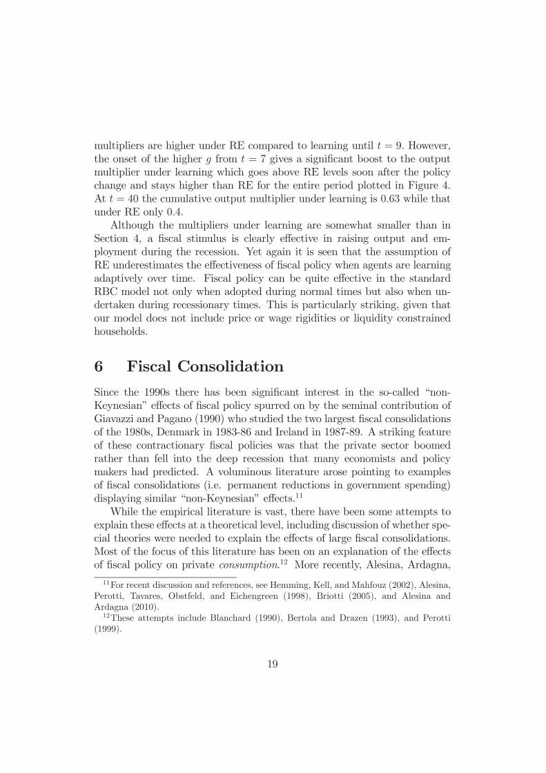
is 20% and that of consumption/output ratio is 59% ˜ is assumed to bedistributed normally with zero mean and standard deviation = 0 007,which is in line with the value used in this literature.Our choice of the gain parameter = 0 04 is in line with most of the

literature, e.g. Branch and Evans (2006), Orphanides and Williams (2007),and Milani (2007). Eusepi and Preston (2011) use a much smaller value forthe gain, but they do not consider changes in policy, for which a larger valueof is more appropriate.For the policy exercises, there is an increase in government purchases from

¯ = 0 20 to ¯0 = 0 21 (a 5% increase) that takes place at = 1, and lasts until= 9, i.e. for eight quarters (e.g. a two-year war) in equation (12). We plot

the mean time paths for each endogenous variable over 100 000 replicationsin Figure 1.Under RE the dynamics are well understood, see Baxter and King (1993)

and Mitra, Evans, and Honkapohja (2011) for details. falls as long as thepolicy change is in e ect and then increases towards the (unchanged) steadystate. falls on impact and then increases monotonically towards the steadystate. An important feature of a temporary increase in is that consumptionsmoothing by agents is achieved by a reduction in investment . The smallwealth e ect due to a temporary, as opposed to a permanent change in ,leads to small impact e ects on , , and . The ratio falls on impactwhich raises and lowers on impact. continues to be low during theperiod of high , and this reduces over time. People maintain a risingpath of by reducing as long as the period of increased lasts, which alsoresults in a falling path of over time. Once the period of high is over, arising path of can be maintained without the need to reduce capital andthere is an investment boom at this point and starts increasing towardsthe steady state. The ratio starts rising, which lowers (raises ),leading to further declines in as it converges towards the steady state.Consider now the impacts of the policy under learning. The most marked

di erence under learning compared to RE is the sharper fall in investmenton impact. Under RE, agents foresee the path of low wages (high inter-

est rates) in the future which reduces initial consumption more on impactcompared to learning. With expectations of future wages and interest ratespre-determined, and only a small rise in (due to the temporary change),the reduction in consumption at = 1 is much smaller under learning thanunder RE. (The impact e ects on other variables are also muted under learn-ing for the same reason). Consequently, there is a sharp fall in with run

13

down rapidly. The sizable negative impact e ect of under RE, followedby a steady return to steady state is sometimes viewed as implausible. Incontrast under learning the response over the rst ve years is hump-shaped,followed by some overshooting and eventual convergence. This hump-shapedresponse is also seen in and .Under learning, although agents correctly foresee the period of higher

taxes, they fail to appreciate the precise form of the wage and price dy-namics that result from the policy change. The reduction in over =1 1 = 8, leads to lower wages and expected wages, , and higherinterest rates and expected interest rates, , resulting in a period of ex-cessive pessimism during the period of high . The resulting reduction inand increase in during this period reverses the fall in and stabilizesin excess of RE levels. Then, when the period of high ends at = 9, theplanned reduction in leads to a sharp spike in and build-up of . Thisleads to a period of higher wages and expected wages, and lower interest ratesand expected interest rates, and thus to an extended period of correction tothe earlier period of overpessimism, before eventual convergence back to thesteady state.One way to view these results is that agents fail to foresee the full impacts

of the crowding out or crowding in of capital from government purchases. Inthe present case, agents tend to extrapolate the low wages during the periodof increased purchases, which result from the run-down of capital. Whileagents understand that their future taxes will fall when the war ends, theyfail to recognize the improvement in wages that will occur after the crowdingin of capital after the war. This is the source of the excessive pessimismduring the war, with a resulting correction after the war ends.We turn now to a comparison of the government purchase multipliers

under RE and learning. As argued by several authors, e.g. Hall (2009), themultipliers obtained in RBC models are too small to be consistent with thedata. Hall notes that US evidence from WWII and the Korean wars suggestmultipliers for GDP in the 0.7 to 1.0 range and Ramey (2011a) concludes thatfor de cit- nanced increases in purchases a range of 0.8 to 1.5 is likely. Thegeneral view is that output multipliers in RBC models are very small, andunlikely to be consistent with these values. As emphasized e.g. by Leeper,Traum, and Walker (2011), Keynesian elements need to be included in themodel to obtain an aggregate demand channel and realistic multipliers. Anissue that has not received attention is the potential role for adaptive learningto provide an additional channel for the multiplier within the standard RBC

14

model. We now take up this issue.Figure 2 shows the results for the output, investment and consumption

multipliers for the policy experiment displayed in Figure 1. In each casewe show both the multiplier viewed as a distributed lag response and thecumulative multiplier over time. For each graph within Figure 2, the RE andlearning responses are shown. The cumulative multipliers are computed asa discounted sum using the discount factor . Speci cally, for the outputmultipliers we compute

=¯

¯0 ¯and =

P=1

1( ¯)

(¯0 ¯)P 1

=11for = 1 2 3

with analogous formulae for the investment and consumption multipliers. Weuse discounting to ensure that, e.g., small persistent values of ¯ do notreceive undue weight. Note that for 1 the (discounted) cumulativeoutput multiplier equals one plus the cumulative consumption multiplier plusthe cumulative investment multiplier.The output multipliers are particularly striking. Although the impact

multiplier is larger under RE than under learning, by quarter 5 the learningmultiplier is larger than the RE multiplier and by quarter 8 the RE multiplieris near zero, where it remains, while the learning multiplier has increasedsubstantially, reaching a peak of over 0 7 in quarter 10. The di erence inmultiplier e ects is captured well by the (discounted) cumulative multiplier,which over ve years is more than 0 8 under learning but less than 0 25under RE. In fact, in the nal period of the gure (year 15), the cumulativeoutput multiplier is 0 94 under learning and only 0 22 under RE. Strikingly,the output multipliers obtained under learning are in line with the empiricalevidence cited above.What accounts for the much larger output multiplier under learning com-

pared to RE? This can be seen from the consumption and investment multi-pliers. Under both RE and learning, the higher crowds out consumption,but there is a hump-shaped response under learning, which declines untilquarter 10. In fact the consumption multiplier eventually (from = 16)turns positive, and the long-run cumulative consumption multiplier is sub-stantially less negative under learning than RE. In the nal period of thegure, the cumulative consumption multiplier is 0 29 under learning and0 47 under RE. That is, overall there is signi cantly less crowding out of

consumption under learning than under RE.

15

The biggest di erence is, however, in the behavior of the investment mul-tipliers. As discussed earlier, the negative impact e ect on investment islarger under learning than under RE, but this quickly reverses and by quar-ter 6 the impact on investment is positive under learning and substantiallynegative under RE. The cumulative investment multipliers after ve yearsare over 0 25 under learning and about 0 4 under RE. Thus, under RE theoverall small cumulative output multiplier re ects crowding out of investmentas well as consumption, while the longer-run cumulative output multipliersunder learning of over 0 94 re ect much less crowding out of consumptionand substantial crowding in of investment.We remark that adaptive learning can shed some light on the controver-

sial issue of the qualitative response of consumption to a rise in governmentpurchases. As noted by Ramey (2011b), some empirical studies nd negativeresponses of private consumption, in the short to medium term, while othersnd positive responses. Under RE, it is well known that the consumptionmultiplier is quite negative in the RBC model, as it is in our Figure 2. AsHall (2009), p. 198, puts it forcefully “The model is fundamentally inconsis-tent with increasing and constant consumption when government purchasesrise.” Our study indicates that under learning the distributed lag response ofconsumption in the RBC model can eventually become positive (in Figure 2,this happens from quarter 16 onwards). Thus, under learning we have botha negative consumption response in the short to medium term and a positiveresponse thereafter.Many authors have demonstrated that the purely neoclassical (RBC)

model has no potential to produce realistic output multipliers because of thesigni cant crowding out of consumption and investment and that in order toget acceptable output multipliers consistent with the empirical evidence, onehas to turn to models that blend neoclassical and Keynesian elements. Evenif one accepts that New Keynesian features are part of a realistic mechanismby which government purchases a ect output, it is useful to understand howlarge the multiplier can potentially be in RBC models as some of the micro-foundations are common in neoclassical and New Keynesian models. Ourprincipal nding is that the introduction of adaptive learning to the RBCmodel can by itself rectify the apparent inability of this model to t theevidence on output multipliers. RBC models with learning are capable ofdelivering higher multipliers and indeed are even within the range found inempirical studies.

16

5 Fiscal Stimulus in Recessions

Temporary increases in government spending are often motivated as policiesto expand output and employment during recessions. A growing literatureis reconsidering their e ectiveness owing to the large scal stimuli adoptedin various countries in the aftermath of the Great Recession. For example,Christiano, Eichenbaum, and Rebelo (2011) and Woodford (2011) demon-strate the e ectiveness of scal policy in models with monetary policy whenthe zero lower bound on nominal interest rate is reached. Although the mainargument for such policies relies on a demand channel, it is clearly of interestto examine the impact of a scal stimulus in the RBC model. We are par-ticularly interested to know if such a policy remains e ective under learningwhen implemented during a severe recession.With this in mind, we consider a situation motivated by events during the

Great Recession in the US. The NBER Business Cycle Dating Committeeestimates December 2007 as the start of the recession and June 2009 asthe trough, after which the economy again began to expand. Thus the USeconomy was in recession during the whole of 2008 and the rst half of 2009.It is widely agreed that the recession was the most severe in the US since theGreat Depression of the 1930s.We model the above situation by assuming that the economy is initially

in a steady state (corresponding to say the last quarter of 2007). We capturethe main features of the Great Recession by the following sequence of events:a sequence of negative two-standard-deviation shocks to the innovation (˜ )hits the economy for four periods in the technology equation 10 (i.e. ˜ =2 in periods = 1 2 3 4).7 This captures the severity of the recession in

2008. This is followed by the economy being hit by negative one-standard-deviation shocks to the innovation ˜ in the next two periods (i.e. ˜ =in periods = 5 6), i.e., the rst half of 2009. Thereafter, from period 7onwards the evolution of the economy is governed by equation (10) with ˜drawn from a zero mean normal distribution with variance 2 with =0 007 as before.Features of the policy change motivated by the American Recovery and

Reinvestment Act (ARRA) of February 20098 are captured in the model by

7Of course, we are using negative productivity shocks to capture the various aspectsof the nancial crisis that presumably reduced productivity in the economy as a whole.More elaborate RBC models would incorporate speci c wedges.

8For a summary of the features of the ARRA, see Romer and Bernstein (2009) and

17

an increase in announced in period = 5. In particular, we assume that at= 5 it is announced credibly that there will be an increase in two quartershence from ¯ = 0 2 to ¯0 = 0 21 (a 5% hike in approximately 1% of GDP)for a period of two and half years i.e. from periods = 7 16 It is alsoannounced that will return to its original level of ¯ from period = 17onwards.The dynamics under learning are shown in Figure 3 for the variablesand (the mean paths over 20 000 replications are reported).9 The

solid black line illustrates the learning paths with the policy change. We alsodepict the learning paths without any policy change with the lighter shadedline. Of course, there are no di erences in the dynamics of the two economiesfor the rst year until the policy change is announced at = 5 The severityof the recession during the rst year means that has fallen by 5 61% asof = 4 Once the policy change is announced at = 5 the dynamics of thetwo economies starts to di er, though the e ect on and for the rst fewperiods is small.The impact of the policy builds up steadily after the policy change comes

into e ect at = 7. rises over time and is approximately 0 68 % pointshigher at = 17. The di erences in dynamics start getting smaller from= 25 onwards but continues to be signi cantly higher with the policy

change for ve years and stays above the no-policy path throughout the 10year period plotted in Figure 3. Employment also gets a substantial boostduring the time of higher and in fact is above the steady state from period11 onwards. The boost in and the lower levels of during the time ofhigher help explain the signi cant expansionary e ects of the scal policyunder learning.10

We also plot the corresponding output multipliers for this policy exper-iment in Figure 4. The left hand panel shows the distributed lag multiplierand the right hand panel the (discounted) cumulative output multipliers. Inthe gure, the solid black line illustrates the multipliers under learning whilethe dashed line are the multipliers under the assumption of RE. The output

Cogan, Cwik, Taylor, and Wieland (2010).9The policy we consider now is an announced anticipated change in that takes place

in the near future. For brevity we do not provide the details for RE and learning and referthe reader to Mitra, Evans, and Honkapohja (2011).10As discussed in Section 4, investment is to some extent crowded out during the rst

part of the implementation, followed by a recovery during the later part of the implemen-tation and a surge as the policy ends.

18

multipliers are higher under RE compared to learning until = 9 However,the onset of the higher from = 7 gives a signi cant boost to the outputmultiplier under learning which goes above RE levels soon after the policychange and stays higher than RE for the entire period plotted in Figure 4.At = 40 the cumulative output multiplier under learning is 0 63 while thatunder RE only 0 4Although the multipliers under learning are somewhat smaller than in

Section 4, a scal stimulus is clearly e ective in raising output and em-ployment during the recession. Yet again it is seen that the assumption ofRE underestimates the e ectiveness of scal policy when agents are learningadaptively over time. Fiscal policy can be quite e ective in the standardRBC model not only when adopted during normal times but also when un-dertaken during recessionary times. This is particularly striking, given thatour model does not include price or wage rigidities or liquidity constrainedhouseholds.

6 Fiscal Consolidation

Since the 1990s there has been signi cant interest in the so-called “non-Keynesian” e ects of scal policy spurred on by the seminal contribution ofGiavazzi and Pagano (1990) who studied the two largest scal consolidationsof the 1980s, Denmark in 1983-86 and Ireland in 1987-89. A striking featureof these contractionary scal policies was that the private sector boomedrather than fell into the deep recession that many economists and policymakers had predicted. A voluminous literature arose pointing to examplesof scal consolidations (i.e. permanent reductions in government spending)displaying similar “non-Keynesian” e ects.11

While the empirical literature is vast, there have been some attempts toexplain these e ects at a theoretical level, including discussion of whether spe-cial theories were needed to explain the e ects of large scal consolidations.Most of the focus of this literature has been on an explanation of the e ectsof scal policy on private consumption.12 More recently, Alesina, Ardagna,

11For recent discussion and references, see Hemming, Kell, and Mahfouz (2002), Alesina,Perotti, Tavares, Obstfeld, and Eichengreen (1998), Briotti (2005), and Alesina andArdagna (2010).12These attempts include Blanchard (1990), Bertola and Drazen (1993), and Perotti

(1999).

19

Perotti, and Schiantarelli (2002) have argued that descriptive evidence sug-gests that increases in private investment (rather than private consumption)explain a greater share of the response of private-sector GDP growth in largescal consolidations.13 They nd very little evidence that private investmentreacts di erently during these large scal adjustments than in the “normal”circumstances. As they remark on p. 586, “This result questions the needfor “special theories” for large versus small changes in scal policy.”Episodes of large scal consolidations are good examples of situations

which economic agents are unlikely to have experienced earlier in their life-times. As argued in the Introduction, in such situations it is plausible toreplace RE by the assumption that agents gradually learn about e ects ofthese policy changes. We will see that the standard RBCmodel with adaptivelearning is able to explain the key features in the behavior of consumptionand investment during these scal episodes.Fiscal consolidations are typically modeled as a surprise permanent re-

duction in government purchases, starting from steady state at = 0. Weconsider the following scenario. At the beginning of period = 1 a pol-icy announcement is made that the level of government purchases will fallpermanently from ¯ = 0 22 to ¯0 = 0 20 (i.e. an almost 10% drop in ).The policy announcement is assumed to be credible and known to the agentswith certainty. We believe this is a realistic assumption; drastic cuts in pur-chases are typically implemented when things turn very bad and the publicunderstands that permanent adjustments are required.The long run e ects on the steady state of a decrease in government con-

sumption are well-known: higher consumption and lower levels of investment,output, labor, and capital. See e.g. Baxter and King (1993).The dynamics under RE are also standard; see for instance Baxter and

King (1993), pp. 321-2, Heijdra (2009), chapter 15, or Mitra, Evans, andHonkapohja (2011). The qualitative dynamics are con rmed by the behaviorof variables under RE in Figure 5. For our purposes, the most relevant issueis the behavior of and . Under RE there is a big rise in on impactovershooting the new (higher) steady state followed by a gradual fall towardsthis steady state. on the other hand, falls dramatically below the new(lower) steady state on impact followed by a gradual rise over time. While

13See also Alesina, Perotti, Tavares, Obstfeld, and Eichengreen (1998). Perotti (1999),footnote 31, concedes that these episodes were characterized by big increases in investment(and net exports).

20

the behavior of is consistent with the scal episodes mentioned above, thebehavior of is at odds with the empirical literature documented above.Under learning rises on impact, followed by a gradual hump-shaped

increase in its level eventually going above the RE level before monotonicallyfalling towards the steady state. The most striking di erence from RE is,however, in the behavior of investment. Instead of the big drop in investmentunder RE, the opposite case of a large boom in investment and hence a risingpath of capital occur under learning in the initial periods after the policychange. Strikingly, this qualitative behavior of under learning is consistentwith the empirical evidence cited above.Why is the behavior of di erent under learning compared to RE? At

= 1, consumption rises because of the decrease in the present value of taxes. As in the case of a temporary change in , discussed in Section 4, the

impact e ects are less under learning than under RE because the paths offuture and are not fully anticipated. Under learning + + graduallyrespond to the data, leading initially to a gradual rise in + (and fall in

+ ) before eventually falling towards the steady state.As a consequence of the smaller sizes of the impacts on output and con-

sumption at = 1, the decrease in necessarily leads to a higher level ofunder learning than under RE, and in fact a sharp increase in investment

follows. In the periods immediately following the policy change, expecta-tions of wages and interest rates begin to adjust. Two factors are at work.The higher capital stock in the periods soon after the policy change leads tohigher forecasts of future wages and lower forecasts of future interest ratesand thus higher and lower . This leads to a further increase in ,and decreases in and , which results in decreases in from its high levelat = 1. After several periods this process moves to an downward path,accompanied by a rise in , and a decrease in , driving downwardsand upwards to their steady state values. The other factor at work isthat over time coe cient estimates under RLS learning gradually adjust inresponse to the shock and the evolution of the data. Eventually the coe -cients converge to the values that correspond to the REE values at the newsteady state, so that in the long run there is convergence to the new REE.Under adaptive learning, the behavior of and are both in line with

the episodes of scal retrenchment cited above. Investment increases sharplyunder learning: in period 1 it is more than 4% points higher than the initialsteady value and continues to stay higher than RE levels for 3 years. growsless rapidly under learning compared to RE levels for six quarters but is then

21

signi cantly above RE levels for a sustained period. These results for andare obtained in the conventional RBC model under learning, without the

need to introduce real frictions or distortionary taxes that are employed inAlesina, Ardagna, Perotti, and Schiantarelli (2002).Table 1 summarizes the impact of learning on the behavior of investment,

consumption and output. For each variable the Table gives, over di erenthorizons, the di erence between the cumulative impact under learning andunder RE. This di erence is particularly striking for investment. For exam-ple, over ve years the cumulative di erence between the level of investmentunder learning and under RE amounts to 6.6% of steady state output or31.9% of steady state investment. Over ve and ten year horizons the cumu-lative e ect on consumption is also greater under learning than under RE.It follows that the cumulative di erence between the level of output underlearning and under RE, which is equal to the sums of the di erences for in-vestment and consumption, is also large over all three horizons. Over tenyears this di erence amounts to over 7.5% of steady state output.It should be noted, however, that scal consolidation leads to a fall in

output and employment under both RE and learning.14 This is an unavoid-able consequence of the lower steady state level that necessarily accompaniesa permanent reduction in in the basic RBC model that we are using. How-ever, falls less rapidly under learning and is around 0 7 of a percentagepoint higher than RE levels after year one. This feature explains the higherlevels of output under learning compared to RE levels for the entire 10 yearperiod depicted in Figure 5 and summarized in Table 1.To summarize, the literature on scal consolidation emphasizes the pos-

sibility of positive e ects on both private consumption and, especially, pri-vate investment resulting from permanent decreases in government spending.Adaptive learning provides a natural mechanism, operating through expecta-tions, for a surge in investment immediately following a scal consolidation.The perceived lower taxes leads to higher consumption and lower employ-ment through the usual wealth e ect. Under learning wages rise less, andinterest rates fall less than they do under RE, so that consumption risesmore gradually and the higher level of personal saving leads to higher levelsof investment over this period.

14Empirical evidence on aggregate e ects is reviwed, e.g., in Briotti (2005) and IMF(2010), chapter 3.

22

7 Conclusion

In this paper we have studied the impact of changes in government purchasesin a standard RBC model with adaptive learning. Methodologically, ourapproach has been to assume that households understand the direct e ectsof announced changes in government purchases on their after-tax income,but have imperfect knowledge of the implications of the policy for the futurepaths of wages and interest rates. Expectations of these latter variables followthe adaptive learning approach in which agents estimate and update theirforecasts using statistical learning rules.Using this approach we study the implications for three inter-related ques-

tions that have been a major focus of recent research. Our main ndingis that the multiplier e ects of government purchases in RBC models un-der learning are much larger than under the standard rational expectationsassumption, and are within the range found in empirical studies. Underadaptive learning there is less crowding out of consumption and there is sub-stantial crowding in of investment. We also nd that scal policy, taking theform of temporary increases in government purchases, is e ective in increas-ing output and employment during severe recessions. Finally, we have seenthat the behavior of both consumption and investment under scal consol-idations better matches the stylized empirical facts when adaptive learningis incorporated into the RBC model.In future work, we aim to study these issues in extended models that allow

for more realistic forms of government nancing, incorporating distortionarytaxes and government debt, and in models that include aggregate demandchannels.

23

References

Aiyagari, R. S., L. J. Christiano, and M. Eichenbaum (1992): “TheOutput, Employment, and Interest Rate E ects of Government Consump-tion,” Journal of Monetary Economics, 30, 73—86.

Alesina, A., and S. Ardagna (2010): “Large Changes in Fiscal Policy:Taxes versus Spending,” Tax Policy and the Economy, 24, 35—68.

Alesina, A., S. Ardagna, R. Perotti, and F. Schiantarelli (2002):“Fiscal Policy, Pro ts, and Investment,” American Economic Review, 92,571—589.

Alesina, A., R. Perotti, J. Tavares, M. Obstfeld, and B. Eichen-green (1998): “The Political Economy of Fiscal Adjustments,” BrookingsPapers on Economic Activity, 1, 197—248.

Auerbach, A., W. G. Gale, and B. H. Harris (2010): “Activist FiscalPolicy,” Journal of Economic Perspectives, 24, 141—164.

Barro, R. J., and R. G. King (1984): “Macroeconomic E ects fromGovernment Purchases and Taxes,” The Quarterly Journal of Economics,99, 817—839.

Barro, R. J., and C. J. Redlick (2011): “Macroeconomic E ects fromGovernment Purchases and Taxes,” The Quarterly Journal of Economics,126, 51—102.

Baxter, M., and R. G. King (1993): “Fiscal Policy in General Equilib-rium,” The American Economic Review, 83, 315—334.

Bertola, G., and A. Drazen (1993): “Trigger Points and Budget Cuts:Explaining the E ects of Fiscal Austerity,” American Economic Review,83, 11—26.

Blanchard, O. J. (1990): “Can Severe Fiscal Contractions be Expan-sionary? A Tale of Two Small European Countries: Comment,” NBERMacroeconomics Annual, 1, 75—111.

Branch, W. A., and G. W. Evans (2006): “A Simple Recursive Forecast-ing Model,” Economic Letters, 91, 158—166.

24

Briotti, M. G. (2005): “Economic Reactions to Public Finance Consoli-dation: A Survey of the Literature,” Occasional paper no.38.

Campbell, J. Y. (1994): “Inspecting the Mechanism: An Analytical Ap-proach to the Stochastic Growth Model,” Journal of Monetary Economics,33, 463—506.

Carceles-Poveda, E., and C. Giannitsarou (2008): “Asset Pricingwith Adaptive Learning,” Review of Economic Dynamics, 11, 629—651.

Christiano, L., M. Eichenbaum, and S. Rebelo (2011): “When is theGovernment Spending Multiplier Large?,” Journal of Political Economy,119, 78—121.

Coenen, G., C. J. Erceg, C. Freedman, D. Furceri, M. Kumhof,R. Lalonde, D. Laxton, J. Linde, A. Mourougane, D. Muir,S. Mursula, C. D. Resende, J. Roberts, W. Roeger, S. Snudden,M. Trabandt, and J. I. Veld (2012): “E ects of Fiscal Stimulus inStructural Models,” American Economic Journal: Macroeconomics, 4, 22—68.

Cogan, J. F., T. Cwik, J. B. Taylor, and V. Wieland (2010): “NewKeynesian versus Old Keynesian Government Spending Multipliers,” Jour-nal of Economic Dynamics and Control, 34, 281—295.

Eusepi, S., and B. Preston (2010): “Central Bank Communicationand Expectations Stabilization,” American Economic Journal: Macroeco-nomics, 2, 235—271.

(2011): “Expectations, Learning and Business Cycle Fluctuations,”American Economic Review, 101, 2844—2872.

Evans, G. W., and S. Honkapohja (2001): Learning and Expectations inMacroeconomics. Princeton University Press, Princeton, New Jersey.

(2011): “Learning as a Rational Foundation for Macroeconomicsand Finance,” mimeo.

Evans, G. W., S. Honkapohja, and R. Marimon (2001): “Conver-gence in Monetary In ation Models with Heterogeneous Learning Rules,”Macroeconomic Dynamics, 5, 1—31.

25

Evans, G. W., S. Honkapohja, and K. Mitra (2009): “AnticipatedFiscal Policy and Learning,” Journal of Monetary Economics, 56, 930—953.

(2011): “Does Ricardian Equivalence Hold When Expectations arenot Rational?,” Working paper nr. 1008, Centre for Dynamic Macroeco-nomic Analysis, University of St Andrews.

Giannitsarou, C. (2006): “Supply-Side Reforms and Learning Dynamics,”Journal of Monetary Economics, 53, 291—309.

Giavazzi, F., and M. Pagano (1990): “Can Severe Fiscal Contractionsbe Expansionary? A Tale of Two Small European Countries,” NBERMacroeconomics Annual, 1, 75—111.

Hall, R. E. (2009): “By HowMuch Does GDPRise If the Government BuysMore Output?,” Brookings Papers on Economic Activity, pp. 183—231.

Heijdra, B. J. (2009): Foundations of Modern Macroeconomics. OxfordUniversity Press, Oxford.

Hemming, R., M. Kell, and S. Mahfouz (2002): “The E ectiveness ofFiscal Policy in Stimulating Economic Activity- A Review of the Litera-ture,” Working paper nr. 02/208, International Monetary Fund.

IMF (2010): World Economic Outlook, October 2010. IMF Publication Ser-vices, Washington, D.C.

King, R. G., C. I. Plosser, and S. T. Rebello (1988): “Production,Growth and Business Cycles,” Journal of Monetary Economics, 21, 195—232.

King, R. G., and S. T. Rebello (1999): “Resuscitating Real BusinessCycles,” in Taylor and Woodford (1999), pp. 927—1007.

Leeper, E. M., N. Traum, and T. B. Walker (2011): “Clearing Up theFiscal Multiplier Morass,” mimeo.

Ljungqvist, L., and T. J. Sargent (2004): Recursive MacroeconomicTheory, Second edition. MIT Press, Cambridge, MA.

26

Long, Jr., J. B., and C. I. Plosser (1983): “Real Business Cycles,”Journal of Political Economy, 91, 39—69.

Marcet, A., and J. P. Nicolini (2003): “Recurrent Hyperin ations andLearning,” American Economic Review, 93, 1476—1498.

Milani, F. (2007): “Expectations, Learning and Macroeconomic Persis-tence,” Journal Of Monetary Economics, 54, 2065—2082.

Mitra, K., G. W. Evans, and S. Honkapohja (2011): “Policy Changeand Learning in the RBC Model,” Working paper nr. 1111, Centre forDynamic Macroeconomic Analysis, University of St Andrews.

Orphanides, A., and J. C. Williams (2007): “Robust Monetary Policywith Imperfect Knowledge,” Journal of Monetary Economics, 54, 1406—1435.

Perotti, R. (1999): “Fiscal Policy in Good Times and Bad,” The QuarterlyJournal of Economics, 114, 1399—1436.

Preston, B. (2006): “Adaptive Learning, Forecast-based Instrument Rulesand Monetary Policy,” Journal of Monetary Economics, 53, 507—535.

Ramey, V. A. (2011a): “Can Government Purchases Stimulate the Econ-omy?,” Journal of Economic Literature, 49, 673—685.

(2011b): “Identifying Government Spending Shocks: It’s All In TheTiming,” The Quarterly Journal of Economics, 126, 1—50.

Romer, C. D., and J. Bernstein (2009): “The Job Impact of the Amer-ican Recovery and Reinvestment Plan,” mimeo.

Sargent, T. J. (1999): The Conquest of American In ation. PrincetonUniversity Press, Princeton NJ.

(2008): “Evolution and Intelligent Design,” American EconomicReview, 98, 5—37.

Taylor, J., and M. Woodford (eds.) (1999): Handbook of Macroeco-nomics, Volume 1. Elsevier, Amsterdam.

Woodford, M. (2011): “Simple Analytics of the Government ExpenditureMultiplier,” American Economic Journal: Macroeconomics, 3, 1—35.

27

TABLE

Cumulative 3 years 5 years 10 yearsE ects in % RLS RE RLS RE RLS RE(P

) ¯ 6 91 6 61 5 28(P

) ¯ 1 09 0 19 2 29(P

) ¯ 5 82 6 80 7 57(P

) ¯ 33 35 31 91 25 48(P

) ¯ 1 84 0 32 3 87

Table 1: Cumulative e ects on key variables of a scal consolidation.Cumulative di erence between e ects under learning (RLS) and under

rational expectations (RE) in percent relative to steady state.

28

10 20 30 40 50 60t

0.4

0.2

0.2

kt

10 20 30 40 50 60t

4

2

2

4

6it

10 20 30 40 50 60t

0.8

0.6

0.4

0.2

ct

10 20 30 40 50 60t

0.2

0.4

0.6

0.8

1.0

1.2nt

10 20 30 40 50 60t

0.2

0.4

0.6

yt

10 20 30 40 50 60t

0.4

0.3

0.2

0.1

0.1

wt

Figure 1: Dynamic paths for a two-year (8 periods) increase in governmentpurchases. The solid lines are the learning paths while the dashed lines arethe RE paths. All variables are measured in percentage deviations fromsteady state values. Mean paths over 100,000 simulations.

29

10 20 30 40 50 60t

0.2

0.4

0.6

ymt

10 20 30 40 50 60t

0.2

0.4

0.6

0.8

ycmt

10 20 30 40 50 60t

0.4

0.3

0.2

0.1

consmt

10 20 30 40 50 60t

0.4

0.3

0.2

0.1

conscmt

10 20 30 40 50 60t

1.0

0.5

0.5

1.0

invmt

10 20 30 40 50 60t

0.4

0.2

0.2

invcmt

Figure 2: Multipliers as a distributed lag response (left hand side) and cumu-lative multipliers (right hand side), for output, consumption, and investment,for the increase in government purchases considered in Figure 1. The solidlines are the learning paths while the dashed lines are the RE paths.

30

10 20 30 40t

6

5

4

3

2

1

yt

10 20 30 40t

5

4

3

2

1

ct

10 20 30 40t

2.0

1.5

1.0

0.5

0.5

1.0

nt

10 20 30 40t

25

20

15

10

5

it

Figure 3: Dynamic paths showing the impact on major variables of a scalstimulus announced in the midst of the Great Recession. Mean paths over20,000 simulations. The solid black line illustrates the learning paths withthe policy change and the lighter shaded line the learning paths withoutthe policy change. All variables are measured in percentage deviations fromsteady state values.

10 15 20 25 30 35 40t

0.1

0.2

0.3

0.4

0.5

0.6

0.7ymt

10 15 20 25 30 35 40t

0.1

0.2

0.3

0.4

0.5

0.6

ycmt

Figure 4: Output multiplier (distributed lag in left hand panel and cumu-lative in right hand panel) for the policy experiment illustrated in Figure3. The solid lines are the learning paths while the dashed lines are the REpaths.

31

10 20 30 40t

4

2

2

4it

10 20 30 40t

0.5

1.0

1.5

ct

10 20 30 40t

2.0

1.5

1.0

0.5

yt

10 20 30 40t

2.5

2.0

1.5

1.0

0.5

nt

10 20 30 40t

0.2

0.4

0.6

0.8

1.0wt

10 20 30 40t

0.08

0.06

0.04

0.02

rt

Figure 5: Dynamic paths for a surprise permanent reduction in governmentspending. The solid lines are the learning paths while the dashed lines are theRE paths. All variables are measured in percentage deviations from steadystate values. Mean paths over 100,000 simulations.

32

www.st-and.ac.uk/cdma

ABOUT THE CDMA

The Centre for Dynamic Macroeconomic Analysis was established by a direct grant from the University of St Andrews in 2003. The Centre facilitates a programme of research centred on macroeconomic theory and policy. The Centre is interested in the broad area of dynamic macroeconomics but has particular research expertise in areas such as the role of learning and expectations formation in macroeconomic theory and policy, the macroeconomics of financial globalization, open economy macroeconomics, exchange rates, economic growth and development, finance and growth, and governance and corruption. Its affiliated members are Faculty members at St Andrews and elsewhere with interests in the broad area of dynamic macroeconomics. Its international Advisory Board comprises a group of leading macroeconomists and, ex officio, the University's Principal.

Affiliated Members of the School

Dr Fabio Aricò. Prof George Evans (Co-Director). Dr Gonzalo Forgue-Puccio. Dr Laurence Lasselle. Dr Seong-Hoon Kim. Dr Peter Macmillan. Prof Rod McCrorie. Prof Kaushik Mitra (Director). Dr Geetha Selvaretnam. Dr Ozge Senay. Dr Gary Shea. Dr Gang Sun. Prof Alan Sutherland. Dr Alex Trew.

Senior Research Fellow

Prof Andrew Hughes Hallett, Professor of Economics, Vanderbilt University.

Research Affiliates

Prof Keith Blackburn, Manchester University. Prof David Cobham, Heriot-Watt University. Dr Luisa Corrado, Università degli Studi di Roma. Dr Tatiana Damjanovic, University of Exeter. Dr Vladislav Damjanovic, University of Exeter. Prof Huw Dixon, Cardiff University. Dr Anthony Garratt, Birkbeck College London. Dr Sugata Ghosh, Brunel University. Dr Aditya Goenka, Essex University. Dr Michal Horvath, University of Oxford. Prof Campbell Leith, Glasgow University. Prof Paul Levine, University of Surrey. Dr Richard Mash, New College, Oxford. Prof Patrick Minford, Cardiff Business School. Dr Elisa Newby, University of Cambridge. Prof Charles Nolan, University of Glasgow. Dr Gulcin Ozkan, York University.

Prof Joe Pearlman, London Metropolitan University. Prof Neil Rankin, Warwick University. Prof Lucio Sarno, Warwick University. Prof Eric Schaling, South African Reserve Bank and

Tilburg University. Prof Peter N. Smith, York University. Dr Frank Smets, European Central Bank. Prof Robert Sollis, Newcastle University. Dr Christoph Thoenissen, Victoria University of

Wellington and CAMA Prof Peter Tinsley, Birkbeck College, London. Dr Mark Weder, University of Adelaide.

Research Associates

Miss Jinyu Chen. Mr Johannes Geissler. Miss Erven Lauw Mr Min-Ho Nam. Advisory Board

Prof Sumru Altug, Koç University. Prof V V Chari, Minnesota University. Prof John Driffill, Birkbeck College London. Dr Sean Holly, Director of the Department of Applied

Economics, Cambridge University. Prof Seppo Honkapohja, Bank of Finland and

Cambridge University. Dr Brian Lang, Principal of St Andrews University. Prof Anton Muscatelli, Heriot-Watt University. Prof Charles Nolan, St Andrews University. Prof Peter Sinclair, Birmingham University and Bank of

England. Prof Stephen J Turnovsky, Washington University. Dr Martin Weale, CBE, Director of the National

Institute of Economic and Social Research. Prof Michael Wickens, York University. Prof Simon Wren-Lewis, Oxford University.

www.st-and.ac.uk/cdma RECENT WORKING PAPERS FROM THE CENTRE FOR DYNAMIC MACROECONOMIC ANALYSIS

Number Title Author(s) CDMA10/13 Economic Crisis and Economic Theory Mark Weder (Adelaide, CDMA and

CEPR)

CDMA10/14 A DSGE Model from the Old Keynesian Economics: An Empirical Investigation

Paolo Gelain (St Andrews) and Marco Guerrazzi (Pisa)

CDMA10/15 Delay and Haircuts in Sovereign Debt: Recovery and Sustainability

Sayantan Ghosal (Warwick), Marcus Miller (Warwick and CEPR) and Kannika Thampanishvong (St Andrews)

CDMA11/01 The Stagnation Regime of the New Keynesian Model and Current US Policy

George W. Evans (Oregon and St Andrews)

CDMA11/02 Notes on Agents' Behavioral Rules Under Adaptive Learning and Studies of Monetary Policy

Seppo Honkapohja (Bank of England), Kaushik Mitra (St Andrews) and George W. Evans (Oregon and St Andrews)

CDMA11/03 Transaction Costs and Institutions Charles Nolan (Glasgow) and Alex Trew (St Andrews)

CDMA11/04 Ordering Policy Rules with an Unconditional

Tatjana Damjanovic (St Andrews), Vladislav Damjanovic (St Andrews) and Charles Nolan (Glasgow)

CDMA11/05 Solving Models with Incomplete Markets and Aggregate Uncertainty Using the Krusell-Smith Algorithm: A Note on the Number and the Placement of Grid Points

Michal Horvath (Oxford and CDMA)

CDMA11/06 Variety Matters Oscar Pavlov (Adelaide) and Mark Weder (Adelaide, CDMA and CEPR)

CDMA11/07 Foreign Aid-a Fillip for Development or a Fuel for Corruption?

Keith Blackburn (Manchester) and Gonzalo F. Forgues-Puccio (St Andrews)

CDMA11/08 Financial intermediation and the international business cycle: The case of small countries with big banks

Gunes Kamber (Reserve Bank of New Zealand) and Christoph Thoenissen (Victoria University of Wellington and CDMA)

www.st-and.ac.uk/cdma CDMA11/09 East India Company and Bank of

England Shareholders during the South Sea Bubble: Partitions, Components and Connectivity in a Dynamic Trading Network

Andrew Mays and Gary S. Shea

CDMA11/10 A Social Network for Trade and Inventories of Stock during the South Sea Bubble

Gary S. Shea (St Andrews)

CDMA11/11 Policy Change and Learning in the RBC Model

Kaushik Mitra (St Andrews and CDMA), George W. Evans (Oregon and St Andrews) and Seppo Honkapohja (Bank of Finland)

CDMA11/12 Individual rationality, model-consistent expectations and learning

Liam Graham (University College London)

CDMA11/13 Learning, information and heterogeneity Liam Graham (University College London)

CDMA11/14 (Re)financing the Slave Trade with the Royal African Company in the Boom Markets of 1720

Gary S. Shea (St Andrews)

CDMA11/15 The financial accelerator and monetary policy rules

Gu ̈neş Kamber and Christoph Thoenissen

CDMA11/16 Sequential Action and Beliefs under Partially Observable DSGE Environments

Seong-Hoon Kim

CDMA12/01 A Producer Theory with Business Risks Seong-Hoon Kim and Seongman Moon

..

For information or copies of working papers in this series, or to subscribe to email notification, contact:

Kaushik Mitra Castlecliffe, School of Economics and Finance University of St Andrews Fife, UK, KY16 9AL

Email: km91@at-andrews.ac.uk; Phone: +44 (0)1334 462443; Fax: +44 (0)1334 462444.