Enhanced Subsurface Interpolation by Geological Cross-Sections by SangGi Hwang, PaiChai University, Korea Abstract Subsurface geological structures, such as bedding, fault planes and ore body, are disturbed by folding and faulting. Mathematical interpolation of the drill core or projected surface geology is not suitable to illustrate such an complex geological structure. A simple graphic algorithm, developed by Visual Basic and GIS components, generates topographic cross-sections and projected intersection points between drill core or surface geology information and the vertical cross-section. The algorithm accounts for inclined drill core geometry as well. In using the topographic cross-section and the point information of the top of the subsurface plane, geological cross-sections are input based on the knowledge of regional geology. The node points of the input sections are being used to interpolate the subsurface plane. For fast calculation, inversed distance weight method is utilized. Kriging method is also tested but it shows no significant difference in geological applications. This application has been tested to model the 3D shape of limestone body. Folded limestone body is clearly displayed and overall shape of the contact surface is more realistic than the simple interpolation resulted from kriging method. This attempt illustrates that the modeling of the subsurface geological planes cannot be relied on the mathematical calculations or unique computer operation alone, and knowledge based input by geologist is critical. Introduction One of the classical geological application is the interpretation of the underground rock structures from limited surface geology. To understand the underground geological structure more clearly, geologists relied heavily on cross-sections. Reliable tools, such as orthographic projections (Hobbs et al, 1976; McIntyre and Weiss, 1956) and map interpretation techniques (Ragan, 1973; Bennison and Moseley, 1997; Hatcher and Hooper, 1990), are available for generation of accurate 3D cross-sections. However, manual application of these methods are rather tedious and require intense care, and therefore, they tend to stay in class rooms. Abruptly changing computer technology opens new applications and methodologies in geology. Recent studies of computerized map analyses methods start to show promising future for the automated 3D cross-section work, more simpler and accurate analyses, and visualization of underground geological structures. These days GIS techniques are becoming common practical tools for geologists. These tools record detailed structural information in spatial data base form. Schetselaar(1995) utilized the digital information for computerized cross-section work. Smith and Gardoll(1997)

proposed a visualizing method of interpolated gridding data of strike and dip measurements. This type of approach can contribute to classify structural domains in a complexly deformed area. DeKemp(1998) pointed out the importance of projection work of the surface geology to underground and proposed projection algorithm for planar and linear features to underground. DeKemp(1999) also applied the Bezier interpolation method to generate smooth feature of the projected subsurface planar and linear structures. Mallet(1997), on the other hand, suggested a discrete modeling method for the 3D interpolation of subsurface structure. Considering the irregularity of the geological structures and physical properties related to the 3D geometrical features, discrete modeling method can be a very reliable tool. Above studies provided some methodologies to build a reasonable cross-section routine as a computer application. One common practice in geology, however, is the derivation of subsurface structure from limited surface feature. If the surface survey would not provide enough information, geologists utilize available drill core, as well as geophysical and outcrop information to build cross-sections, and extrapolate the underground 3D geological structure from those sections. During the process, geologists are forced to judge the most reasonable interpretation of the nature of the subsurface structure. Therefore, the final 3D interpretation of the subsurface geological structure is a product of experience driven state of the art by geologists. This is particularly true in an area where the outcrops are scarce. This aspect has been overlooked from mathematical geology because it is considered to be interpretive judgement and it does not contain technical or scientific methodology. The current study intends to present a simple methodology which can easily be implanted in a computer s/w for the computer aided geological cross-section routine. Methodology If the given data in an area is insufficient, interpreting a 3D subsurface geological structure by simple interpolation could seriously be misleading. Suppose a folded layer is cut by a reverse fault and the fold axes dips horizontally (Fig.1), and if one gained depth information of the top of the layer from drill cores, simple interpolation of the top layer position would be very different from reality as shown in Fig. 1. If the subsurface structure is complex and the drill space is wider, such discrepancy would be even larger. If the spacing between the drill cores are reduced, one can achieve more realistic 3D interpolation of the underground structure. Reducing the core space could easily be achieved if cross-section information between the drill cores is added to the surface map. Using CAD or GIS components, cross-sections could be drawn as vector lines. All vector lines record the vertex points and the coordinates of the vertex points can be converted to the 3D geographic coordinates. Attitudes of the bedding planes from the surface survey are reflected while the cross-sections are drawn. Therefore, the converted vertex points from cross-section are the best deduced 3D points which are laying on the interpolating surface. When the cross-section points are incorporated into the map, these points can be used as extra depth information, and cross-sections through these extra points can be drawn. If enough points through such cross-sections are drawn, these

points could be interpolated by kriging or inverse distance weight methods.

Fig.1 A schematic block diagram of folded and faulted area. Four drill core positions are illustrated. A surface defined by the red line is the interpolated result from the drilled depth information. Some complexity might occur if the interpolated surface has irregular shape. Mushroom shape object has more than one depth point at one map point. Curvilinear interpolation models cannot account for more than one depth information at one map point. If a layer is translated by reverse fault, near the fault zone could have more than one depth points for a stratigraphic boundary. To avoid this problem, one can divide 3D domains and record the interpolated grid information accordingly. In this case, boundary condition of domains must be defined clearly. Modeling a limestone layer at Jechen area, Korea Fig. 2A illustrates 9 drill core locations in a limestone quarry at the Jechen area, Korea. The drillings were not always vertical, and in fact, some of the drillings were horizontal (Fig. 2B). Surface geology indicates the layers are folded and the fold axes shallowly plunges to north-west. To model the 3D shape of the limestone layer, depth to the top surface of the limestone layer is recorded from the core information. Top surface positions of the limestone layer are calculated from the orientation of the drill core and the core length, using cylindrical coordinate. On the map view, top surface positions from each drill core are shifted from the drill position, due to the inclined nature of the drill core (Fig.3). Interpolation of these coordinates is performed by kriging method with linear semi variogram model. Fig. 4 illustrates the 3D model with the topographic surface. The model plane intersects topographic surface and the modeled surface does not reflect the underground geological structure as illustrated in Fig.4. This explains how critical and important to have sufficient data points in

constructing a realistic 3D model. A.

B.

Fig.2. Surface geology and the drill core information of Jechen area, Korea. A. Map view. B. 3D view of the drill cores.

Fig. 3. Projections of the core depths to the map view 3D points. The two core are drilled horizontally and the drilled azimuth is 250 degree. Red dots, aligned parallel to the drill azimuth, are the position of the limestone layer boundary. These dots have 3D coordinates.

Fig. 4. The modeled folded layer from surface geology and drill core information. Small inlet at the lower left corner illustrates the modeled folded surface by cross-sections. The red surface is a modeled plane by sparse drill core information only.

Cross-sections of 4 lines are constructed as in Fig. 5. While the sections are constructed, the lithological boundary, attitude of bedding and axial planes, and depth information from the drill core are considered. Vertex points of the limestone boundary on the cross-section are converted to geographic coordinate points and they are plotted as 3D points as in Fig. 5A. To increase the density of the depth points, extra cross-sections are constructed, using the 3D points, which are obtained from previously constructed cross-sections (Fig. 6). After the extra cross-section information are gathered (Fig.7), moving window operation is used to interpolate the depth grid of the limestone surface (Fig.4).

Fig. 5.A. Cro

poscorpoi

B. Crobla

Fig. 6in the

A.

Cross-sections from the know drillss-section localities. Along the croition, medium size dots indicate the, and small dots indicate the convnts. ss-sections drawn from known dri

ck dots. Thick red line is the modele

. Additional cross-sections construcfigure) from previously drawn cross

B.

core information. ss-section line, big dots indicate the drill core e converted 3D elevation points from the drill erted 3D elevations from cross-section vertex

ll core depth information which are marked as d plane.

ted using the converted vertex points (circles -sections (Fig. 5).

Fig. 7. Plotted depth points from additional cross-sections. While the additional cross-sections are constructed, previously constructed cross-section vertex points are used for indexing the depth of the model surface. Soft Ware To draw cross-sections easily, a s/w is developed using AutoCad and ActiveX components. The s/w includes the 3 major routines; interpolation, database, and graphic routine for map and cross-section drawing. Kriging and inverse distance weight methods are used to interpolate the height data from 3D points. AutoCad ActiveX routine (SelectionSet) is utilized to select the data groups in the circular window area. Drill core information and the structural data are stored in Access, and the database is connected to the AutoCad graphic objects. Graphic routines are built by the ActiveX components. Map drawing algorithm includes coordinate conversion, from latitude and longitude or TM to UTM, DEM generation, and geological symbol plotting routine. Basic maps, such as 3D vector type topographic map and the locations of mining tunnels, can be drawn by ordinary AutoCad 3D polylines (Fig. 8). To construct the topographic grid and automatic elevation reading routine, DEM generation routine from the vector map is built. Since the 3D polyline object of the AutoCad records vertex points at internal database, the vertex points could be read by selecting the polyline object, and the vertexes could be converted to the 3D point objects on the map as in Fig. 9. Moving window of given size scans the map area with given spacing. While the window scans, data points in the window area are selected and the elevation of the central point of the window is interpolated by inverse distance weight method. The

kriging method was also tested, but it took much more time and did not show any significant difference in results. Calculated DEM array is stored in binary file. Drawing routine of the 3D polylines for topographic grid is built. After the topographic grid is

constructed, 3D geometry of the area can be illustrated as in Fig. 4. Fig. 8. The 3D presentation of the mining tunnels and drill directions, using AutoCad.. Topographic grids are 3D polylines, tunnel and drill objects are shaded.

Fig. 9. Converted 3D points from the vertex points of the polylines of the vector topographic map. The inlet area at lower right corner illustrates details of the point map.

Structural geology information and the coordination of the outcrop position are recorded in database as in Fig. 10. A routine is built to read each line of structural geology table (Fig. 10B) sequentially, and through the primary key field, location of the structural data is read from the station table (Fig.10A). Shapes for the symbol type, such as bedding and foliation are built, and the routine plots the rotated symbol of structural data. While the symbol is plotted, database information, such as station number and attitude, are recorded into the AutoCad�s external database.

.

B

A.

Fig. 10. Database tables for the cross-section routine. A. Station table records the UTM coordinates for outcrops. B. Structural geology table records features of structural elements and their orientation. The cross-section drawing routine is divided into 3 steps. The first step converts depth information of the drill core into the 3D points on the map. Cross-section line can be decided from the distribution of elevation points and localities of the structural data, such as bedding, fold axes, and lithologic boundaries. The routine begins by displaying selected drill core columns for stratigraphic correlation (Fig. 11). User must assign subjective layer boundary from the column graphically, then the computer reads points on the column and calculate the intersection 3D point between the core column and the stratigraphic or geological structural boundary. Calculated 3D points are plotted on the map as in Fig. 3.

Fig. 11. Drill core column drawing for stratigraphic correlation. Depth information of the column are read from database. All boundaries, selected by user from this column, are projected underground parallel to the orientation of the core, and are plotted on the map as in Fig. 3. The second step is to draw basic information for cross-section drawing. User must decide the position of section line and input all available data. For example, x-section1 in Fig. 5A is decided because one can find lithologic boundary, structural data and drill core information along this line. Topographic shape is read from DEM as drawn as in Fig.5B. Already projected points, such as depth of the layer, are plotted on the section, and known surface feature, such as attitude of bedding and fold geometry, are projected to underground. The projection method is the same as Schetselaar(1995) and DeKemp(1998) and the short line is extended from the topographic surface on the 2D section. The short line and depth points on the 2D section are simply referenced information which can be used for cross-section drawing. Once the basic information is drawn, user must construct the cross-section as in Fig. 5B. The third step converts the vertex points of the 2D cross-section to the geographic 3D coordinates and insert the converted 3D points into the map (Fig. 6). After enough sections from known information are drawn, the reference points can be used to draw further sections as in Figs. 6 and 7. Through the above process, enough 3D points, for underground DEM calculation, can be acquired (Fig. 7) and a subsurface grid as in Fig. 4 can be drawn using the same interpolation routine mentioned earlier. The final routine is the graphic display in AutoCad. Shading and 3D view routine display the final drawing very effectively.

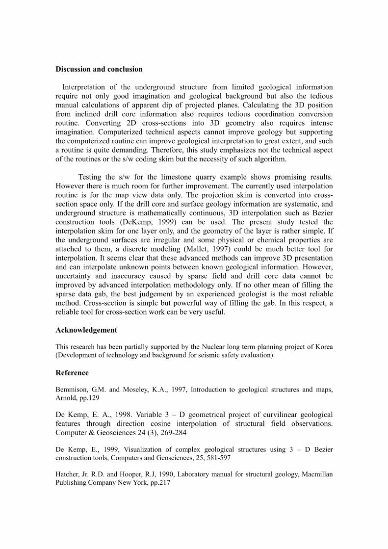
Discussion and conclusion

Interpretation of the underground structure from limited geological information require not only good imagination and geological background but also the tedious manual calculations of apparent dip of projected planes. Calculating the 3D position from inclined drill core information also requires tedious coordination conversion routine. Converting 2D cross-sections into 3D geometry also requires intense imagination. Computerized technical aspects cannot improve geology but supporting the computerized routine can improve geological interpretation to great extent, and such a routine is quite demanding. Therefore, this study emphasizes not the technical aspect of the routines or the s/w coding skim but the necessity of such algorithm. Testing the s/w for the limestone quarry example shows promising results. However there is much room for further improvement. The currently used interpolation routine is for the map view data only. The projection skim is converted into cross-section space only. If the drill core and surface geology information are systematic, and underground structure is mathematically continuous, 3D interpolation such as Bezier construction tools (DeKemp, 1999) can be used. The present study tested the interpolation skim for one layer only, and the geometry of the layer is rather simple. If the underground surfaces are irregular and some physical or chemical properties are attached to them, a discrete modeling (Mallet, 1997) could be much better tool for interpolation. It seems clear that these advanced methods can improve 3D presentation and can interpolate unknown points between known geological information. However, uncertainty and inaccuracy caused by sparse field and drill core data cannot be improved by advanced interpolation methodology only. If no other mean of filling the sparse data gab, the best judgement by an experienced geologist is the most reliable method. Cross-section is simple but powerful way of filling the gab. In this respect, a reliable tool for cross-section work can be very useful. Acknowledgement This research has been partially supported by the Nuclear long term planning project of Korea (Development of technology and background for seismic safety evaluation). Reference Bemmison, G.M. and Moseley, K.A., 1997, Introduction to geological structures and maps, Arnold, pp.129 De Kemp, E. A., 1998. Variable 3 � D geometrical project of curvilinear geological features through direction cosine interpolation of structural field observations. Computer & Geosciences 24 (3), 269-284 De Kemp, E., 1999, Visualization of complex geological structures using 3 � D Bezier construction tools, Computers and Geosciences, 25, 581-597 Hatcher, Jr. R.D. and Hooper, R.J, 1990, Laboratory manual for structural geology, Macmillan Publishing Company New York, pp.217

Hobbs, B.E., Means W.D., Williams P.F, 1976, An outline of structural geology, John Wiley and Sons, pp.571 Mallet J. L., 1996, Discrete Modeling for Natural Object, Mathematical Geology, Vol. 29, No. 2, 199 � 219 McIntyre, D.B. and Weiss L.E., 1956, Construction of block diagrams to scale in orthographic projection. Geological Assoc., Proc., 67, pts. 1 and 2, pp142-155 Ragan, D.M., 1973, Structural geology, An intruduction to geometrical techniques, John Wiley and Sons, pp.208 Schetselaar, E. M., 1995. Computerized field-data capture and GIS analysis for generation of cross section in 3-D perspective views. Computer & Geosciences, 21(5), 687-701 Smith, A. B., Gardoll, S. J., 1997. Structural analysis in mineral exploration using a geographic information system adapted stereographic-projection plotting program. Australian Journal of Earth Science, 44, 445-452