Engineering Tools for Robust Creep Modeling - VTT · VTT PUBLICATIONS 728 Engineering Tools for...
139
Dissertation VTT PUBLICATIONS 728 Stefan Holmström Engineering Tools for Robust Creep Modeling
Transcript of Engineering Tools for Robust Creep Modeling - VTT · VTT PUBLICATIONS 728 Engineering Tools for...

Dissertation VTT PUBLICATIONS 728VTT CREATES BUSINESS FROM TECHNOLOGYTechnologyandmarketforesight•Strategicresearch•Productandservicedevelopment•IPRandlicensing•Assessments,testing,inspection,certification•Technologyandinnovationmanagement•Technologypartnership
•••VTTPUB
LICA
TION
S728ENG
INEER
ING
TOO
LSFOR
RO
BU
STCR
EEPMO
DELIN
G
ISBN 978-951-38-7378-3 (soft back ed.) ISBN 978-951-38-7379-0 (URL: http://www.vtt.fi/publications/index.jsp)ISSN 1235-0621 (soft back ed.) ISSN 1455-0849 (URL: http://www.vtt.fi/publications/index.jsp)
Stefan Holmström
Engineering Tools for Robust Creep Modeling
Creep models are needed for design and life management of structural components operating at high temperatures. The determination of creep properties require long-term testing often limiting the amount of data. It is of considerable interest to be able to reliably predict and extrapolate long term creep behavior from relatively small sets of creep data. In this thesis tools have been developed to improve the reliability of creep rupture, creep strain and weld strength predictions. Much of the resulting improvements and benefits are related to the reduced requirements for supporting creep data. The simplicity and robustness of the new tools also make them easy to implement in analytical and numerical solutions. Creep models for selected high temperature steels and OFP copper are presented.


VTT PUBLICATIONS 728
Engineering Tools for Robust Creep Modeling
Stefan Holmström
Dissertation for the degree of Doctor of Science in Technology to be pre-sented with due permission of the Faculty of Engineering and Architecture, The Aalto University School of Science and Technology, for public exami-nation and debate in K216 at Aalto University (Otakaari 4, Espoo, Finland)
on the 5th of February, 2010, at 12 noon.

ISBN 978-951-38-7378-3 (soft back ed.) ISSN 1235-0621 (soft back ed.)
ISBN 978-951-38-7379-0 (URL: http://www.vtt.fi/publications/index.jsp) ISSN 1455-0849 (URL: http://www.vtt.fi/publications/index.jsp)
Copyright © VTT 2010
JULKAISIJA UTGIVARE PUBLISHER
VTT, Vuorimiehentie 5, PL 1000, 02044 VTT puh. vaihde 020 722 111, faksi 020 722 4374
VTT, Bergsmansvägen 5, PB 1000, 02044 VTT tel. växel 020 722 111, fax 020 722 4374
VTT Technical Research Centre of Finland, Vuorimiehentie 5, P.O. Box 1000, FI-02044 VTT, Finland phone internat. +358 20 722 111, fax + 358 20 722 4374
Technical editing Mirjami Pullinen Edita Prima Oy, Helsinki 2010

3
Stefan Holmström. Engineering Tools for Robust Creep Modeling [Virumismallinnuksen uudet mene-telmät]. Espoo 2010. VTT Publications 728. 94 p. + 53 p.
Keywords creep, strain, damage, modeling, steel, OFP copper
Abstract High temperature creep is often dealt with simplified models to assess and pre-dict the future behavior of materials and components. Also, for most applications the creep properties of interest require costly long-term testing that limits the available data to support design and life assessment. Such test data sets are even smaller for welded joints that are often the weakest links of structures. It is of considerable interest to be able to reliably predict and extrapolate long term creep behavior from relatively small sets of supporting creep data.
For creep strain, the current tools for model verification and quality assurance are very limited. The ECCC PATs can be adapted to some degree but the uncer-tainty and applicability of many models are still questionable outside the range of data. In this thesis tools for improving the model robustness have been devel-oped. The toolkit includes creep rupture, weld strength and creep strain model-ing improvements for uniaxial prediction. The applicability is shown on data set consisting of a selection of common high temperature steels and the oxygen-free phosphorous doped (OFP) copper. The steels assessed are 10CrMo9-10 (P22), 7CrWVMoNb9-6 (P23), 7CrMoVTiB10-10 (P24), 14MoV6-3 (0.5CMV), X20CrMoV11-1 (X20), X10CrMoVNb9-1 (P91) and X11CrMoWVNb9-1-1 (E911).
The work described in this thesis has provided simple yet well performing tools to predict creep strain and life for material evaluation, component design and life assessment purposes. The uncertainty related to selecting the type of material model or determining weld strength factors has been reduced by the selection procedures and by linking the weld behavior to the base material mas-ter equation. Much of the resulting improvements and benefits are related to the reduced requirements for supporting creep data. The simplicity and robustness of the new tools also makes them easy to implement for both analytical and nu-merical solutions.

4
Stefan Holmström. Engineering Tools for Robust Creep Modeling [Virumismallinnuksen uudet mene-telmät]. Espoo 2010. VTT Publications 728. 94 s. + liitt. 53 s.
Keywords creep, strain, damage, modeling, steel, OFP copper
Tiivistelmä Rakenteiden suunnitteluun ja elinikäennusteisiin käytetyt kuumalujien terästen lujuusarvot ja hitsien lujuuskertoimet pohjautuvat virumiskoetuloksiin, joita on varsinkin pitkäaikaisina käytettävissä usein vain niukasti. Sen vuoksi on erityi-sen tärkeää, että koetuloksiin sovitetut materiaalimallit ovat taloudellisia, tarkko-ja ja luotettavia erityisesti ekstrapoloitaessa pidemmille käyttöajoille.
Tässä väitöstyössä on kehitetty uusia malleja työkaluiksi virumismurtolujuu-den, hitsien lujuuskertoimien ja virumisvenymän luotettavaan määrittämiseen sekä virumiseliniän ennustamiseen erityisesti tapauksissa, joissa mallinnuksen tueksi on käytettävissä niukasti virumiskoetuloksia. Uusien mallien suoritusky-kyä on testattu eurooppalaisessa vertailututkimuksessa, jossa ne ennustivat yk-sin-kertaisesta muodostaan huolimatta venymiä tarkemmin kuin aiemmat ja huomattavasti monimutkaisemmat virumismallit. Uusia malleja on työssä sovel-lettu OFP-kuparille ja ferriittisille teräksille 10CrMo9-10 (P22), 7CrWVMoNb9-6 (P23), 7CrMoVTiB10-10 (P24), 14MoV6-3 (0.5CMV), X20CrMoV11-1 (X20), X10CrMoVNb9-1 (P91) ja X11CrMoWVNb9-1-1 (E911). Materiaali-malleja on myös sovitettu numeerisen suunnittelun työkaluihin (COMSOL ja ABAQUS) ja verifioitu pitkään käytössä olleen hitsatun putkiyhteen elinikätar-kastelulla.
Väitöstyön tuloksena kehitettyjä malleja ja menetelmiä voivat soveltaa korke-an lämpötilan rakenteiden suunnittelijat ja eliniän hallinnan asiantuntijat helpot-tamaan ja tarkentamaan virumiskäyttäytymisen ennustamista. Työn keskeinen anti on kehitettyjen menetelmien tarjoama vähentynyt materiaalidatan tarve ja mallien yksinkertainen rakenne, joka helpottaa niiden hyödyntämistä sekä ana-lyyttisissä että numeerisissa ratkaisuissa.

5
Preface This work has been carried out at VTT, financially supported by the Academy of Finland grant 117700 with prof. Kim Wallin acting as instructor. It has been supervised by prof. Hannu Hänninen, head of laboratory of Engineering Materi-als at Helsinki University of Technology (HUT). Prof. Hänninen is greatly ac-knowledged for his valuable input in the finalization stage of the thesis and for arranging a place at HUT to escape the hectic work surroundings of VTT.
A substantial part of the research gone into the development of the creep mod-els and modeling tools has been done over several years within many VTT pro-jects, both national and international. Projects like Extreme (internal VTT), Aloas (RFCS), LC-Power & Life-Power (Tekes financed), The Värmeforsk pro-ject on Creep damage development in welded X20 and P91 components and the LEIA / PIKE projects, to name a few, have contributed to this thesis.
The European Creep Collaborative Committee (ECCC) has been a valuable supply of interesting challenges, creep expertise, relevant feed-back, active sup-port, friendship and an invaluable source of creep data that would not have been accessible without the ECCC WG1 network lead by Dr. Stuart Holdsworth. The Japanese creep data produced and freely distributed by NIMS has also been a valuable source of high quality data. The work done on the OFP copper for nu-clear waste canisters has been part of the national projects LEIA / PIKE, funded by the public Nuclear Waste Management Program in Finland (KYT).
Special thanks go of course to the co-authors of the publications incorporated in this thesis. Also my team, Materials performance for combustion systems, has given me great support and has shown incredible patience and has not complained over sloppily done administrative tasks during the final stages of this work.
Finally, I would like to thank my wife and children for their valuable support and understanding when my eyes have glazed over at home, in the car or at some social event, brooding over some nutty creep modeling detail.

6
Contents Abstract ................................................................................................................. 3 Tiivistelmä ............................................................................................................. 4 Preface.................................................................................................................. 5 Research hypothesis and original features........................................................... 7 List of abbreviations and symbols....................................................................... 11 1. Introduction ................................................................................................... 15 2. General aspects on creep data, modeling and design ................................. 18
2.1 Creep testing..................................................................................................................... 28 3. Creep rupture modeling ................................................................................ 37
3.1 Post assessment testing ................................................................................................... 41 3.2 Non-conservatism in creep rupture modeling ................................................................... 43 3.3 Creep rupture models for ferritic steels............................................................................. 45 3.4 Creep rupture model for oxygen-free phosphorus doped copper..................................... 49 3.5 Rupture models for welds and weld strength factor.......................................................... 55
3.5.1 Rigidity Parameter Correction engineering tool for improved WSF calculation ... 58 3.5.2 Sensitivity analysis of P91 steel weld strength factor....................................... 61
4. Creep strain modeling................................................................................... 63 4.1 Manson-Haferd-Grounes (MHG) strain model engineering tool for creep strain
prediction .......................................................................................................................... 67 4.2 Logistic Creep Strain Prediction (LCSP) engineering tool for robust creep strain
prediction .......................................................................................................................... 69 5. Multi-axial creep strain and damage............................................................. 73
5.1 Engineering tool multi-axial LCSP for FEA .................................................................... 74 5.1.1 The FEA COMSOL implementation ................................................................. 74 5.1.2 The FEA ABAQUS implementation.................................................................. 75
5.2 Engineering tool multi-axial exhaustion parameter........................................................ 75 6. Discussion..................................................................................................... 78 7. Conclusions................................................................................................... 82 8. Summary....................................................................................................... 84 References.......................................................................................................... 85 Appendices
Papers IVII
Appendices II, III, V and VI of this publication are not included in the PDF version. Please order the printed version to get the complete publication (http://www.vtt.fi/publications/index.jsp).

7
Research hypothesis and original features
The hypothesis of this thesis is that there are possibilities (simple tools) for by-passing many of the difficulties in establishing creep properties for materials, especially those caused by insufficient amount of (available) data. The problem with scarce or insufficient data is encountered even for well established steels. The public domain availability of relevant models or creep strain data excluding the simplest Norton law approaches or Monkman-Grant relationships are diffi-cult to come by. The engineering tools developed in this thesis (presented in Table 1) are all original contributions to the benefit of simplifying and enhanc-ing the creep property determination (rupture, strain, multi-axial response).
Table 1. List of engineering tools developed in the scope of this thesis and their main usage.
TOOL USAGE RPC Rigidity Parameter Correction
Method for testing creep-rupture model flexibility. Determines the susceptibility of conservatism in extrapolation. Can also be used for determination of conservative weld strength factors [1], [2].
MHG Manson-Haferd-Grounes creep strain model
Simple parametric creep strain model, based on strain data only [3].
LCSP Logistic Creep Strain Prediction strain model
Robust creep strain model, based on rupture model and a curve shape function. Gaining accuracy with increasing availability of strain data [4], [5].
Λ-filter Multi-axial damage pa-rameter
Method of visualizing creep exhaustion (consumed multi-axial creep strain factor) in FEA modeling implemented with multi-axial form of LCSP model [6], [7].

1. Introduction
8
The developed tools can be utilized for the prediction of weldment creep life, creep strain and even multi-axial creep damage. The models are in themselves robust, meaning that similar reliability can be expected from the predictions as would be expected from creep rupture models. The best feature is, however, that this is accomplished utilizing a minimum amount of data. Some of the strain models presented have been verified with creep data withheld from the initial model optimization. The LCSP together with the Λ-filtering method for visualiz-ing creep damage in FEA simulations has shown great potential in predicting creep damage evolution. The Λ-filtering tool can be used as a stand-alone feature with any FEA creep model. The special tool developed for rationalizing the weld strength factor calculation (RPC) is also (as the LCSP) based on the base material strength giving a better mathematical capability for extrapolation purposes.
The engineering approach and the deliberate aim of keeping the model-ing tools simple will hopefully make them more attractive to the design en-gineer and the life management expert. The simplicity, accuracy and ro-bustness in prediction are in itself the driving force and ultimate aim of this work.

9
List of publications and authors contribution
The scientific papers of this thesis are:
I Holmström, S. & Auerkari, P. Effect of short-term data on predicted creep rupture life pivoting effect and optimized censoring. Materials at High Temperatures, Vol. 25 (2008) 3, September, pp. 103109, North-ampton, UK: Science Reviews 2000 Ltd.
II Holmström, S. & Auerkari, P. Predicting weld creep strength reduction for 9% Cr steels. International Journal of Pressure Vessels Piping, Vol. 83 (2006) 1112, pp. 803808.
III Holdsworth, S. R., Askins, M., Baker, A., Gariboldi, E., Holmström, S., Klenk, A., Ringel, M., Merckling, G., Sandstrom, R., Schwienheer, M. & Spigarelli, S. Factors influencing creep model equation selection. Interna-tional Journal of Pressure Vessels and Piping, Vol. 85 (2008) 12, pp. 8088.
IV Holmström, S. & Auerkari, P. Robust prediction of full creep curves from minimal data and time to rupture model. Energy Materials, Materials Sci-ence & Engineering for Energy Systems, Vol. 1 (2006) 4, pp. 249255, Maney Publishing.
V Holmström, S. & Auerkari, P. Predicting creep rupture from early strain data. Materials Science and Engineering: A, Vol. 510511 (2009), pp. 25−28.
VI Holmström, S., Laukkanen A. & Calonius, K. Finding critical damage lo-cations by Λ-filtering in FE modeling of a girth weld. Materials Science and Engineering: A, Vol. 510511 (2009), pp. 224228.
VII Holmström, S., Laukkanen, A., Rantala, J., Kolari, K., Keinänen, H. & Lehtinen, O. Modeling and verification of creep strain and exhaustion in a welded steam mixer. Journal of Pressure Vessel Technology, Vol. 131 (2009), 061405 (5 pages).

1. Introduction
10
Pertti Auerkari the co-author in most of the papers (I, II, IV & V) is an ex-tremely experienced senior research scientist with over 30 years of experience in creep research. His contribution is an important one in all the papers he co-authors, namely his never-ending enthusiasm, guidance to the core questions of the creep problem at hand and especially in the noble art of formulating sound conclusions.
Paper III, with a number of authors, written by Dr. Stuart Holdsworth, is based on the round robin results of the creep strain modeling efforts of the ECCC. In this paper the work done on the Manson-Haferd-Grounes (MHG) strain model and its performance is contributed by the present author, and the rest is the ex-cellent work of my colleagues from the ECCC network.
Paper IV is the central paper of the thesis, combining the rupture model of P22 (10CrMo9-10) steel with a creep curve shape function into a creep strain model. The results of this paper are utilized and implemented in all the rest of the thesis papers (VVII).
In Paper V the LCSP is successfully applied to predict long-term creep behav-ior (strain and rupture) for oxygen-free phosphorus doped copper (OFP).
In Paper VI the LCSP is implemented in COMSOL finite element code and used for predicting creep damage (with the Λ-filter) in a simple girth weld case. My co-author Anssi Laukkanen contributed with the LCSP coding, the meshing of the weld, running the simulations and by sharing his FEA expertise. Kim Ca-lonius made comparison runs for the same structure using the Norton law strain model in ABAQUS.
In Paper VII a more complicated welded component is assessed with LCSP and the Λ-filter. For this paper my co-author Kari Kolari made the ABAQUS implementation with input from both Anssi Laukkanen and me. The mesh and simulation runs were made by Kari Kolari and Heikki Keinänen. Juhani Rantala coordinated the work and Olli Lehtinen was the utility contact person contribut-ing with all the needed background information.

11
List of abbreviations and symbols
MCM Minimum commitment method (nonlinear with instability parameter A)
MC Minimum commitment method (multi-linear without instability parameter)
PLM Larson-Miller model
MH Manson-Haferd model
A Instability parameter of the nonlinear Minimum commit-ment method
A Norton law constant (considered temperature dependent)
K Intercept of the Monkman-Grant relationship
r Slope of the Monkman-Grant relationship
OFP Phosphorus doped oxygen-free copper
WSF Weld strength factor
SRF Stress reduction factor
TRF Time reduction factor
tr Time to rupture
trd Time to rupture (data)
trm Time to rupture (model)
tε Time to strain
ε Strain
εc Creep strain •
ε Strain rate (1/h)

1. Introduction
12
m
•
ε Minimum (or steady state) creep rate (1/h)
ε0 Initial strain (strain after loading of a creep test)
εf Creep failure strain
εfu Uniaxial creep failure strain
εfm Multi-axial creep failure strain •
sε Strain rate in strain control (SSRT testing) •
tε Strain rate in stress control (SSRT testing)
A Dimensionless factor (Norton law)
B Rate coefficient
D Diffusion coefficient
E Elastic modulus
b Burgers vector
d Grain size
p Exponent for grain size dependence (Norton law)
p LCSP parameter
σ Stress (in MPa)
σUTS Ultimate tensile stress
Qc Activation energy for creep
Qc* Activation energy for creep (Wilshire)
n Norton stress exponent
T(K) Temperature (in Kelvin)
k Constant in Wilshire equation
u Constant in Wilshire equation
tr Time to rupture
R Gas constant
dtd /σ Rate of stress relaxation
α Parameter for SSRT testing (approx. 0.75)
η Reference parameter in indentation creep testing
P Mean pressure under indenter (indentation creep)

13
∆ Displacement (indentation creep test)
d Indenter width (indentation creep test)
β Reference parameter (indentation creep test)
FSP Test load (small punch testing)
KSP Material constant (small punch testing)
h Thickness of specimen (small punch testing)
rSP Radius of the punch indenter (small punch testing)
RSP Radius of the receiving hole (small punch testing)
C Larson-Miller and LCSP constant
Z Data scatter parameter
RMS Root mean square
SSE Standard error of estimate
PAT Post assessment test
f(σ) Stress function (log(σ) or σx)
P(σ) Manson-Brown stress function
Ru/t/T Rupture strength, time t and temperature T
Ru(W)/t/T Rupture strength for weld, time t and temperature T
LF Life fraction
HAZ Heat affected zone
trR RCP corrected rupture time
trm Model rupture time
tp Pivot point for RPC model
R Rigidity parameter
xo and p Fitting parameters in LCSP
Λ Lambda filter designation
h Hydrostatic stress

1. Introduction
14

1. Introduction
15
1. Introduction Creep is often dealt with using properties and models based on small data set or by using old classical approaches. The shortcomings related to the determination of creep strength or creep strain are mainly due to the nature of creep. Since it is a time-dependent damage mechanism it naturally requires long-term testing to give reliable strength values. For instance the reliable extrapolation range is con-sidered to be a factor of three times the longest test duration in the data set repre-senting the material. This leads to a requirement for testing beyond 30 000 h to cover a design life of 100 000 h. Most conventional power plants are designed for 200 000 h of service. Creep is also an expensive property to determine. Al-ternative shorter term tests have of course been proposed, but the classical long-term constant load creep test is still considered by most materials experts to be the only test incorporating time-dependent material degradation needed for reli-able long term life management. The creep properties (mainly rupture strength) used in design of high temperature components are based on standardized strength values given in standards such as the EN10216-2 [8]. These standard-ized values are mean material values and material scatter of ±20% in stress can be expected. It is to be remembered that the final strength values (published in standards) are average values from several assessments performed by experts using different modeling tools, not always in agreement with each other. In the end, the values are agreed on by the expert group preparing the standard. As a consequence the strength values are seldom directly retrievable from any spe-cific creep model. Also, it has happened quite frequently that the standard strength values, especially for new steel grades, have had to be corrected down-ward after obtaining more long-term test data or severe damage has been found in service, as was the case for P122 steel in Japan.
For a new steel to become standardized is a long process. The first-time quali-fications may include a minimum of 2 to 3 isotherms with 35 rupture points not

1. Introduction
16
less than 1030 kh. The PED directive (EU 1997) allows the use of any interna-tionally recognized standard for dimensioning and safety factors of components operating in the creep regime. If a material intended for a component design cannot be selected from a standard it has to pass acceptance or material ap-praisal. The final strength values (in standards) are, as previously stated, the result of many assessments reaching consensus.
When looking for material creep properties the designer or life management researcher is usually confronted with the dilemma of lacking data. For some materials the only easily accessible data available might be the standard (mean) creep strength values such as rupture stress for 10 000, 100 000 or 200 000 hours at specified temperatures,. These are in themselves usually already extrapolated values (in time) by a factor of close to three. Sometimes, in rare cases, both rup-ture and creep strain data can be found but then again it seems that the data from different sources inevitably leads to a situation showing wide scatter in the data between different material batches and testing laboratories. The problem of creep design and creep life prediction and management seems to always return to the critical question of available data and what can be derived from it. In conclusion it is nearly always a challenging task to produce robust predictions (or models) for creep strain or creep rupture for arbitrary high temperature conditions.
The ECCC has with its work on harmonization of creep rupture assessments developed an evaluation method (Post assessment testing or PATs) that enables the assessor to understand and to weigh the quality of the result of the model fit. It also allows the assessor to produce reliable and credible creep strength predic-tions, suitable for inclusion into European standards. Some of these tests are also suited for testing the creep strain model fits. The tools of this thesis are exten-sions and model improvements meant to be used in addition to the ECCC PATs for optimal benefit in material creep modeling.
In literature there is a multitude of creep strain and creep rupture models for creep life and creep strain prediction [9]. However, in most cases the data used for the models is not published and the resulting models require many, in some cases as much as 26 fitting parameters to describe the creep response [10], [11]. In these cases it is almost impossible to validate the models and the resulting possible error in extrapolation. Though it is common sense to avoid using mod-els where the range of data or the accuracy of the models is unknown, it might be the only one available.
By finding simple robust modeling alternatives that require a minimum amount of data (and that can easily be verified) will make structural integrity

1. Introduction
17
calculations more accurate, especially for new materials at an early stage of their development. The same applies for less known or materials where the material data has been kept unpublished due to business reasons. For instance, state-of-the-art gas turbine blading material data seems to be especially difficult to ac-cess. Simplicity and robustness of the creep strength and strain models will con-tribute to safe design and life management of new and existing high temperature components.
In this thesis tools for creep data set structure optimization, creep modeling and implementation techniques for creep life assessment have been developed. The creep response (rupture and/or strain) of high temperature steels such as P22 [12], [13], [14], P23 [15], 0.5CMV [16], X20 [17], P91 [18] and E911 [1], [2] have been studied.
The selected materials represents well the historic development of the heat re-sistant steels from the 530550°C temperature range materials (low alloy steels P22 and 0.5CMV) to those suitable for the intermediate range 550580°C (911Cr steels P91 and X20). Also, a material intended for the higher steam values in the temperature range 580620°C has been assessed (E911, the European not so successful version of the grade 92 steel).
Model development has also been successfully done for oxygen-free phospho-rus doped copper (OFP) [19] to be used in nuclear waste disposal canisters. This material is obviously not a fossil fuel high temperature material but shows the applicability of the thesis engineering tools on a highly complicated modeling case with an extreme extrapolation need for the range of service life.
The binding link between the articles in this thesis is the clear path from sim-ple uniaxial rupture modeling towards more complex structures such as welds and creep strain modeling, culminating in the creep life assessment of a creep damaged weld region of a power plant mixing tank (thesis Paper VII and [20]). The main steps and the papers included in this thesis are presented in the order of increasing modeling complexity, towards the goal of large complex compo-nent creep life multi-axial FEA modeling.

2. General aspects on creep data, modeling and design
18
2. General aspects on creep data, modeling and design Creep is commonly encountered for metals (and alloys) at temperatures roughly above half of the melting point. In general, creep refers to time-dependent de-formation (strain) accumulated under load. From a macroscopic (and engineer-ing) point of view creep is often treated as time-dependent plastic deformation and both elastic and viscous strain components are usually neglected. Ashby [21] proposed that there are six independent deformation mechanisms: defect-free flow, dislocation glide, dislocation creep, volume diffusion flow and twin-ning. The contribution to deformation is very limited for twinning and it is usu-ally not represented in deformation mechanism maps. The deformation maps describe the steady state flow (strain rates) at specified temperature and stress (see Fig. 1). This means that they are representing the mean (model) interpolated or extrapolated minimum strain rates based on measured creep strain data.

2. General aspects on creep data, modeling and design
19
Fig. 1. Schematic deformation mechanism map (no actual material) with minimum creep rates [9].
The strain data acquired from the most common creep tests, the constant load (or stress) tests, is classically divided into three characteristic stages (see Figs 23).
tr
εf
I II III
TIME
STR
AIN
ε0
Fig. 2. Classical creep curve with primary (I) creep stage starting at loading with instanta-neous strain (ε0), secondary (II) stage with the minimum creep rate and tertiary (III) stage ending in rupture (at time tr with a fracture strain εf).
2. General aspects on creep data, modeling and design
20
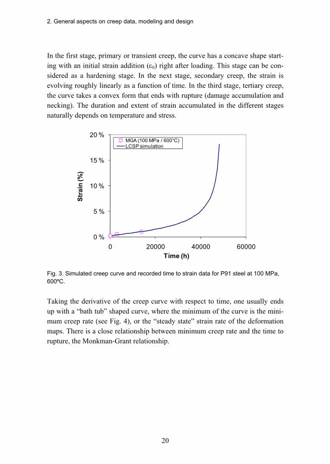
In the first stage, primary or transient creep, the curve has a concave shape start-ing with an initial strain addition (ε0) right after loading. This stage can be con-sidered as a hardening stage. In the next stage, secondary creep, the strain is evolving roughly linearly as a function of time. In the third stage, tertiary creep, the curve takes a convex form that ends with rupture (damage accumulation and necking). The duration and extent of strain accumulated in the different stages naturally depends on temperature and stress.
0 %
5 %
10 %
15 %
20 %
0 20000 40000 60000
Stra
in (%
)
Time (h)
MGA (100 MPa / 600°C)LCSP simulation
Fig. 3. Simulated creep curve and recorded time to strain data for P91 steel at 100 MPa, 600ºC.
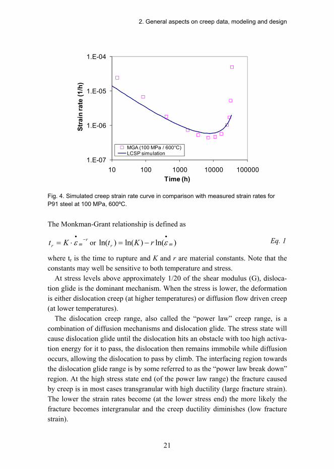
Taking the derivative of the creep curve with respect to time, one usually ends up with a bath tub shaped curve, where the minimum of the curve is the mini-mum creep rate (see Fig. 4), or the steady state strain rate of the deformation maps. There is a close relationship between minimum creep rate and the time to rupture, the Monkman-Grant relationship.
2. General aspects on creep data, modeling and design
21
1.E-07
1.E-06
1.E-05
1.E-04
10 100 1000 10000 100000
Stra
in ra
te (1
/h)
Time (h)
MGA (100 MPa / 600°C)LCSP simulation
Fig. 4. Simulated creep strain rate curve in comparison with measured strain rates for P91 steel at 100 MPa, 600ºC.
The Monkman-Grant relationship is defined as
rmr Kt −
•
⋅= ε or )ln()ln()ln( mr rKt•
−= ε Eq. 1
where tr is the time to rupture and K and r are material constants. Note that the constants may well be sensitive to both temperature and stress.
At stress levels above approximately 1/20 of the shear modulus (G), disloca-tion glide is the dominant mechanism. When the stress is lower, the deformation is either dislocation creep (at higher temperatures) or diffusion flow driven creep (at lower temperatures).
The dislocation creep range, also called the power law creep range, is a combination of diffusion mechanisms and dislocation glide. The stress state will cause dislocation glide until the dislocation hits an obstacle with too high activa-tion energy for it to pass, the dislocation then remains immobile while diffusion occurs, allowing the dislocation to pass by climb. The interfacing region towards the dislocation glide range is by some referred to as the power law break down region. At the high stress state end (of the power law range) the fracture caused by creep is in most cases transgranular with high ductility (large fracture strain). The lower the strain rates become (at the lower stress end) the more likely the fracture becomes intergranular and the creep ductility diminishes (low fracture strain).

2. General aspects on creep data, modeling and design
22
For a creep model to produce accurate results in extrapolation the macroscopic (modeled) strain response should be based on physical simplified functions able to cover the complex interplay of microstructural and sub-microstructural changes interpreted by the micro-mechanisms controlling the creep rate and thereby the measured strain accumulation. However, even though the materials science has been able to produce sufficiently accurate models linking the high temperature microstructural and macroscopical materials response for pure met-als, the more complex high temperature materials still seem to be beyond reach.
The modeling tools developed and all the data assessed within the scope of this thesis are targeted at solving the challenges of the dislocation creep range. Also, most high temperature engineering structures such as steam lines, boilers, turbines operate in this. However, some extrapolations, such as the low stress service conditions of the high temperature steam mixer assessed is approaching diffusion flow dominated conditions and the data assessed at high stress for the nuclear spent fuel copper canister is again crossing over into the power law break down range.
The diffusion flow range, usually divided into Nabarro-Herring creep at higher temperatures and Coble creep at lower temperatures has not been studied in closer detail in this thesis. The Nabarro-Herring creep deformation progresses through the diffusion of atoms and vacancies. Coble creep again progresses through mass and vacancy diffusion along grain boundaries where diffusion can occur at lower energy levels. This is also a reason why Coble creep is more pronounced for fine grain size materials than in coarse grain ones. Both Coble creep and Nabarro-Herring creep produce voids (creep cavitation) or cracks at grain boundaries. For all the mechanisms, the creep rate is controlled by activation energy.
A number of models taking dislocation theory as a basis have been proposed, but they are in most cases better suited for pure metals and not for complex high temperature steels that are highly dynamic and not in thermodynamic equilib-rium. For pure (OFHC) copper a model has recently been introduced, stating no fitting parameters. Though, already when very small amounts of phosphorus are added to the material (<60 ppm), the model shows inconsistencies, that seem difficult to overcome with the attempted scaling factors only [22].
Traditionally the minimum strain rate in the dislocation creep range is de-scribed by the extended Norton law expression of Eq. 2. The stress exponent n for minimum creep rate
•
mε will normally range within 35 for high temperature power law creep and within 57 for low temperature power law creep in the classical expression for polycrystalline metals:

2. General aspects on creep data, modeling and design
23
)/exp()/()/()/( kTQEdbkTDEbA cnp
m −⋅⋅⋅=•
σε , Eq. 2
where A is a dimensionless factor, D the diffusion coefficient, E the elastic modulus, b the Burgers vector, d the grain size, p the exponent for grain size dependence, σ is the applied stress, k the Boltzmanns constant and Qc the acti-vation energy for creep.
For Coble (grain boundary diffusion) and Nabarro-Herring (volume diffusion) creep the corresponding stress exponent n is 1. However the grain size exponent p changes from 3 to 2 when moving towards volume diffusion.
The mechanism related diffusion coefficients for high temperature power law creep and Nabarro-Herring creep are lattice diffusion and for the lower tempera-ture power law creep and Coble creep it is pipe diffusion and grain boundary diffusion, respectively.
The main difficulty in utilizing the above equation in modeling complex high temperature steels, and especially in extrapolation, is that the stress exponent n and the activation energy Qc tend to change at stress levels and temperatures relevant for service conditions. The stress and temperature dependence of n and Qc is shown in Fig. 5 for the grade 91 steel (P91) assessed in this thesis.
15 10 50.5
1
1.5
2
2.5
log(strain rate)
log(
stres
s)
1 .05 1.1 1.15 1.210
8
6
4
1000/(T +273)
log(
strai
n ra
te)
Qc=470 kJ/mol
Qc=680 kJ/moln=7.7
n=2.2
Fig. 5. Presentation of the changing nature of the stress exponent n (at 575°C) and the apparent activation energy Qc (at 100 MPa) for P91 steel (LCSP simulated).
Modifications of the classical power law stress dependency have been proposed in the threshold stress concept and the internal stress concept. These methods rationalize the oversized stress exponents common for the complex high tem-perature steels. The determination of the additional stress variable though re-quires iterative exponent data fitting or sudden short term force reductions dur-

2. General aspects on creep data, modeling and design
24
ing creep testing. The increased uncertainty in parameter determination and the increased complexity of the creep testing has not encouraged the usage of these methodologies in greater extent.
The recent introduction of the Wilshire equations [23] has provided a simple effective competitive methodology for strain rate, time to strain and time to rup-ture assessments. The method though needs additional tensile test data to ac-company the constant load tests. The method is normalizing the creep test stress with yield or ultimate tensile strength at the temperature in question and plotting against either
•
mε ⋅exp(-Q*c/RT) for minimum strain rate data or tr⋅exp(-Q*
c/RT) for rupture data. The model avoids the varying stress exponent n and the activa-tion energy is definable in a straight forward, simple way. Note, however, that that Q*
c ≠ Qc of Eq. 2. The Wilshire equation for time to rupture tr (note in seconds) at stress σ (MPa)
and temperature T (K) is expressed as: u
crTS RTQtk )]/exp([)/ln( *−−=σσ , Eq. 3
where k and u are constants obtained by fitting to the test data, Qc* is the appar-
ent activation energy and σUTS is the tensile strength at the specified temperature. The equation for strain rate is identical to Eq. 3 with tr replaced by
•
mε . Application of this model obviously requires data from both creep rupture
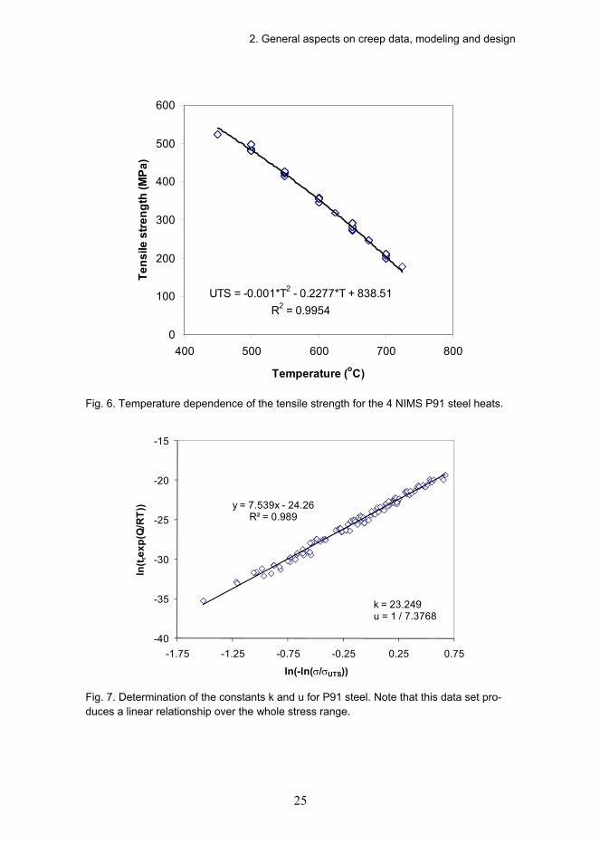
testing and tensile testing. An example of a Wilshire model assessment for time to rupture is presented for P91 steel with data from NIMS [24] in Figs. 68.
The Wilshire equation has been thoroughly tested for several materials includ-ing bainitic rotor forgings of 1Cr-1Mo-0.25V steel [25], martensitic steels P91, P92 and P122, Waspalloy, aluminum alloys and for OFP copper (thesis Paper V).
2. General aspects on creep data, modeling and design
25
UTS = -0.001*T2 - 0.2277*T + 838.51R2 = 0.9954
0
100
200
300
400
500
600
400 500 600 700 800
Temperature (oC)
Tens
ile s
treng
th (M
Pa)
Fig. 6. Temperature dependence of the tensile strength for the 4 NIMS P91 steel heats.
y = 7.539x - 24.26R² = 0.989
-40
-35
-30
-25
-20
-15
-1.75 -1.25 -0.75 -0.25 0.25 0.75
ln(t r
exp(
Q/R
T))
ln(-ln(σ/σUTS))
k = 23.249u = 1 / 7.3768
Fig. 7. Determination of the constants k and u for P91 steel. Note that this data set pro-duces a linear relationship over the whole stress range.

2. General aspects on creep data, modeling and design
26
The main benefit found for the model is that heat to heat data scatter is re-duced by the normalization. The heat to heat data scatter is related to differences in the creep properties due to alloying, heat treatments, product forms and manu-facturing routes for the tested material heats. Also, the mathematical form is inherently more stable at lower stress levels than for traditional time to rupture models with polynomial stress dependence. The equation also gives rupture times that tend to zero when approaching the ultimate tensile strength and values that tend to infinity when the stress approaches zero. The data scatter reduction in the above presented P91 assessment is shown in Figs. 910.
0.1
1
1E-16 1E-14 1E-12 1E-10 0.00000001
tf*exp(Q/RT)
σ/ σ
UTS
MgC-plateMGCMGAMGB
Fig. 8. The Wilshire master curve for P91 steel with Q*c= 300 kJ/mol. The designations MGA, MGB and MGC are pipe, tube and plate heats.

2. General aspects on creep data, modeling and design
27
2
2.5
3
3.5
4
4.5
5
2 3 4 5OBSERVED LIFE, log(h)
PRED
ICTE
D L
IFE,
log(
h)
lgtr*tp=tatp=ta·Ztp=ta/Zta·2tp=ta·½
Fig. 9. Predicted times to rupture against the observed rupture times using the Wilshire equation with calculated tensile strength. The scatter is low (scatter factor Z=2.34, see Eq. 18 for definition).
2
2.5
3
3.5
4
4.5
5
2 2.5 3 3.5 4 4.5 5
OBSERVED LIFE, log(h)
PRED
ICTE
D L
IFE,
log(
h)
lgtr*tp=tatp=ta·Ztp=ta/Zta·2tp=ta·½
Fig. 10. Predicted times to rupture against the observed rupture times using the best parametric equation, in this case Manson-Brown 4th degree stress function f(σ)= σ0.75. The scatter factor is larger than in Fig. 9, Z=3.59 mainly due to badly fitting short term data.

2. General aspects on creep data, modeling and design
28
2.1 Creep testing
The most common type of creep data is the constant load rupture data. The data consists of time to rupture values at specified applied loads at specified tempera-tures. Another common creep data type is closely related to the rupture data, namely the same constant load test including strain measurement (continuous or interrupted test). The constant load creep test is specified in EN 10291 [26]. In the Annex C of the same document the method of estimating the uncertainty of the measurement in accordance with the ISO "Guide to the expression of uncer-tainty in measurement" is presented. The EN ISO 7500-2 [27] specifies the crite-ria for the measurement and calibration of static uniaxial creep testing machines.
Today most constant load creep tests are performed in single specimen dead weight lever machines with continuous displacement measurement (see Fig. 11). However, in Germany rupture and interrupted creep strain tests are still per-formed in multi-specimen creep furnaces. This method produces large amounts of data, but the quality of temperature control and the acquired strain curves are somewhat inferior to the ones acquired by single specimen machines.
In the test type comparison work done in Germany [28] it was shown that the influence of interruptions is weak, always inside the scatter band of uninter-rupted testing. For the steel P22 it was shown that the interrupted tests had a strain factor of around 1.055 in comparison to the uninterrupted tests.
The assessments and models presented in this thesis are solely based on the creep strain and time to rupture data produced with single or multi specimen constant load testing machines.
To get an impression on the data scatter expected in creep data assessments, raw creep rupture data and standard table data (EN 10216-2 [29]) are plotted together with two rupture master curves optimized on the standard in Fig. 12.

2. General aspects on creep data, modeling and design
29
Fig. 11. Constant load creep testing machine assembly. A) Creep specimen ridges for extensometers (displacement measurement), B) Loading weights, C) Upper pull rod, D) Furnace, E) Lever mechanism (1:10), F) Displacement transducer, G) Temperature con-troller, H) Data acquisition computer.
10
100
1000
10 100 1000 10000 100000 1000000
Time to rupture (h)
Str
ess
(MPa
)
EPRI raw dataVGB raw dataEN-10216 standard dataManson-Brown modelW ilshire modelEPRI weld data
Fig. 12. EPRI and VGB data for X20 steel at 600°C with time to rupture models (classical Manson-Brown and Wilshire) optimized on EN-10216 creep strength data.

2. General aspects on creep data, modeling and design
30
Data scatter, encountered in different magnitude for all creep test data, is mostly caused by material specific differences such as heat specific differences in compo-sition, product form or heat treatment. The data scatter will of course play a sig-nificant role in the modeling, adding to the uncertainty of the extrapolations done.
When dealing with creep strain curves one should keep in mind that in some reports the creep curves are given with and in others without the instantaneous strain. Looking at creep rupture data, for instance isothermally plotted, the be-havior can be divided into three different types. The pure materials normally behave quite linearly in a log-log plot. The creep mechanism might, however, quite suddenly change (the slope changes) at low stress levels. Most ferritic high temperature steels show gradual creep mechanism change over the whole stress range giving the isothermal curves a bent shape. The high temperature steels assessed in this thesis belong mainly to this group (see Fig. 13, for example).
10
100
1000
1000 10000 100000 1000000 10000000
Time (h)
σ (M
Pa)
500 °C 520 °C 550 °C 570 °C
Fig. 13. Rupture model isotherms 500570 ºC for 0.5CMV steel based on stress to speci-fied rupture time tables [30].
Some martensitic steels show sigmoidal behavior, the strength gradually de-creasing in a limited stress range and then stabilizing again. The sigmoidal be-havior is especially conspicuous for the 11CrMoVNb steel assessed in an ECCC round robin yet to be published but shortly presented in the 2009 ECCC confer-ence in Switzerland. These kinds of material data sets are especially difficult for

2. General aspects on creep data, modeling and design
31
both time to rupture and strain modeling. The pre-assessed 11CrMoVNb steel rupture model is presented in Fig. 14.
0
0.1
0.2
0.3
0.4
0.5
0.6
0.7
0.8
0.9
100 1000 10000 100000
Time (h)
σ/U
TS
ave
29
30
31
32
33
34
Fig. 14. Sigmoidal rupture model (open points) for 600ºC isotherm based on normalized stress for 6 heats of 11CrMoVNb steel.
The most common creep test types are presented in Table 2 together with some comments on data availability. The short descriptions of the different testing types are included in the thesis, though not utilized as data sources, for the pur-pose of determining the possibility of withdrawing uniaxial creep parameters from them.
The stress relaxation tests are performed at constant total strain and as creep strain accumulates, the elastic strain component of the total strain decreases, leading to a decreasing stress [31]. The relaxing stress is monitored on-line until it stabilizes and the rate of change becomes insignificant. An example of a re-laxation sequence in a low cycle fatigue test is presented in Fig. 15.
An estimate of the (constant load) secondary creep rate can theoretically be determined from the relaxation test, as a function of stress, when initially load-ing the sample sufficiently to pass the region of primary creep.

2. General aspects on creep data, modeling and design
32
Table 2. Creep test types.
Test type Data type and availability
Constant load / Time to rupture - The most common data type - Standard data tables / standards
Constant load / Creep strain (+rupture) - Full raw data creep curves are rare - For some steels data tables for specified stress, strain and time are available
Constant stress / Creep strain (+rupture) - As above but even more rare
Relaxation test - Data mainly for bolting steels - Difficult to relate to standard creep properties
Slow strain rate test - SSRT (= Constant strain rate test - CSRT)
- Often used for combined creep / envi-ronment testing - Usually not very long durations - Offset in strain rate comp. to creep strain data
Notched bar creep test
- Notch sensitivity tests (limited) - For determining notch weakening/ strengthening - For defining skeletal point multi-axial representative rupture stress
Small punch creep test
- Made in increasing amount - Small samples from service exposed components - Weld zone testing - Relationship to standard creep data not well defined (requires FEA)
Impression creep test - Limited data published - Mainly used in UK - Gives primary / secondary creep
Component testing: - internal pressure - internal pressure + tensile load
- Very limited - Interaction and combined damage

2. General aspects on creep data, modeling and design
33
Fig. 15. Creep relaxation curve extracted from a hold period in a low cycle fatigue (LCF) test for low alloy steel P23 (creep resistant modification of P22) strained to 0.2% at 575ºC [32].
The plastic (creep) strain rate •
pε can then be determined from the equation:
)/(/1 dtdEp σε −=•
, Eq. 4
where E is the Youngs modulus and dtd /σ the measured rate of stress relaxa-tion. It is, however, to be noted that for some materials, in the later stages of relaxation, recovery might become significant leading to lower calculated strain rates than would be measured from corresponding conventional creep tests. An alternative practice of stress relaxation testing is the multi-specimen model-bolt test, where the relaxed stress is measured by means of strain gauges during unloading after long-term creep exposure. Guidelines are found in the ECCC recommendations (2005, Vol. 3) and in the European standards EN 10319-1 [33] and 2 [34]. To date there are no formally recognized procedures for assessing the stress relaxation data, but it is used by some assessors as a fast method for comparing of service exposed materials [35] to virgin material properties. To accurately determine the creep strain exhaustion level, or consumed creep life fraction from these tests would be beneficial for assessing creep fatigue tests
2. General aspects on creep data, modeling and design
34
with holding times. The LCSP model developed will in the near future be used for this purpose.
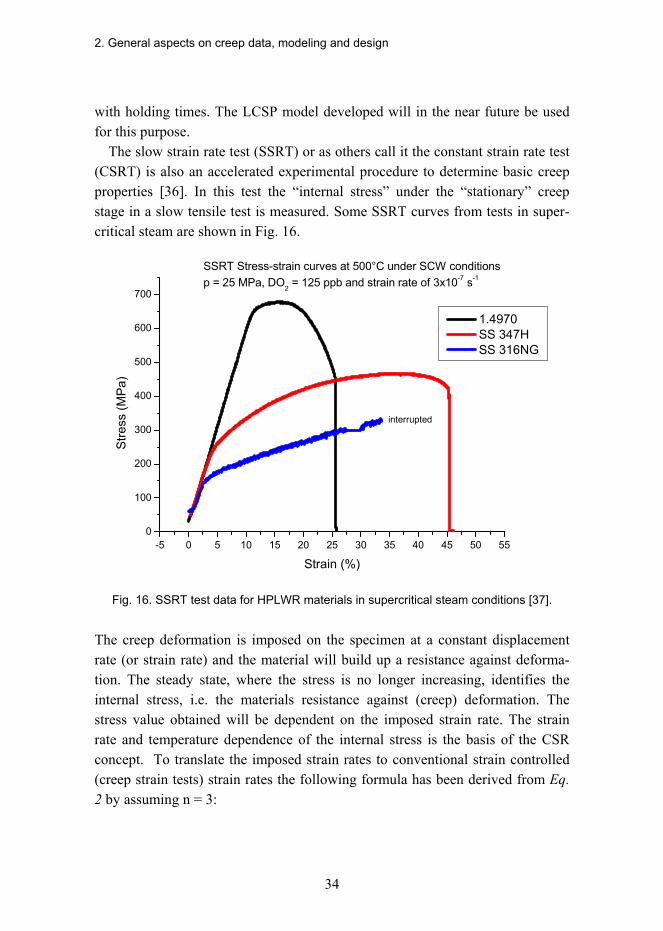
The slow strain rate test (SSRT) or as others call it the constant strain rate test (CSRT) is also an accelerated experimental procedure to determine basic creep properties [36]. In this test the internal stress under the stationary creep stage in a slow tensile test is measured. Some SSRT curves from tests in super-critical steam are shown in Fig. 16.
-5 0 5 10 15 20 25 30 35 40 45 50 550
100
200
300
400
500
600
700
interrupted
SSRT Stress-strain curves at 500°C under SCW conditionsp = 25 MPa, DO2 = 125 ppb and strain rate of 3x10⁻⁷ s-1
Stre
ss (M
Pa)
Strain (%)
1.4970 SS 347H SS 316NG
Fig. 16. SSRT test data for HPLWR materials in supercritical steam conditions [37].
The creep deformation is imposed on the specimen at a constant displacement rate (or strain rate) and the material will build up a resistance against deforma-tion. The steady state, where the stress is no longer increasing, identifies the internal stress, i.e. the materials resistance against (creep) deformation. The stress value obtained will be dependent on the imposed strain rate. The strain rate and temperature dependence of the internal stress is the basis of the CSR concept. To translate the imposed strain rates to conventional strain controlled (creep strain tests) strain rates the following formula has been derived from Eq. 2 by assuming n = 3:

2. General aspects on creep data, modeling and design
35
••
⋅= ts εαε 3 , Eq. 5
where •
sε is the strain rate in strain control and •
tε in stress control. The diffi-culty in determining the true value of the α-parameter (usually approximately 0.75) has been a drawback of this testing type, and has therefore not acquired high popularity among creep experts. An increased use of this creep testing type is foreseen for extreme environments where time is essential for the cost of test-ing, such as supercritical steam autoclave testing, in-core nuclear test reactor testing or material screening for Generation IV nuclear test reactor coolant envi-ronments. The most promising materials could then be tested for long-term creep under constant load. Also for this testing type the LCSP creep strain model will be attempted for improving the determination of the α-parameter.
Impression creep [38][39][40] is a relatively new testing technique developed for local (micro-region) creep properties such as weld zones. The impression creep testing technique involves the application of a steady load to a flat-ended rectangular indenter placed on the surface of a material at the required test tem-perature. Creep allows the indenter to push its way into the surface of the mate-rial. The displacement-time plot is related to the creep properties of the small volume of material in the immediate vicinity of the indenter.
The stress σ related to the creep properties sought is calculated from:
P⋅= ησ , Eq. 6
where P is the mean pressure under the indenter and η reference parameter. The accumulating creep strain ε from the displacement of the indenter follows the equation;
d⋅∆
=β
ε , Eq. 7
where ∆ is the displacement, d the indenter width and β a reference parameter. In [41] the equivalent uniaxial stress was determined to be 0.296 times the mean indenter pressure (= η) and the effective gauge length 0.755 times the indenter width (= β). The creep strain rates in the primary and secondary creep can be obtained with this method. The primary and secondary creep properties deter-mined with the indenter will be utilized for determining the shape functions (LCSP) for in service materials and material zones difficult to test due to re-

2. General aspects on creep data, modeling and design
36
stricted size (such as heat affected zones). These can then be transferred to FEA simulations of complex structures.
The small punch creep test (SP) [42] is like the impression creep test based on small or miniature specimens. The SP specimens are discs 0.250.5 mm thick and 810 mm in diameter. The SP technique was first introduced in the USA and Japan in the 80s. In recent years it has become more widely used also in Europe. The drawback of the method is that the results have to be correlated between the puncher load and the corresponding uniaxial creep test stress.
This relationship is dependent on the radius of the punch indenter, the thick-ness of the test disc, the radius of the receiving hole, and the material under test. A standardization initiative for the SP test method has been put forward in a Code of Practice (CoP) or CEN Workshop Agreement, CWA 15627 [43] pub-lished in December 2006.
In the CoP the ratio of SP test load FSP to the uniaxial creep stress σ is:
hrRKF
SPSPSPSP ⋅⋅⋅⋅= − 2.12.033.3
σ, Eq. 8
where r is the radius of the punch indenter, h is the thickness, R is the radius of the receiving hole, and KSP is a material constant. The LCSP strain model im-plementation for FEA could readily be utilized for the decoding of the SP indenter movement towards better compliance with standard uniaxial creep curves.
Notched bar creep test [44] is also covered by a CoP, issued in 1991. The test was developed for establishing the multi-axial creep stress-rupture properties. The CoP was updated in 2001, to enable the extraction of multi-axial creep strain response. The notched bar test can also be implemented for the determina-tion of local creep strain properties in a weld [45]. The thesis tools such as the FEA implemented LCSP model together with the multiaxial creep exhaustion parameter could improve the understanding of notch sensitivity and creep dam-age accumulation.

3. Creep rupture modeling
37
3. Creep rupture modeling Since creep is time dependent the determination of creep properties is time con-suming and therefore also expensive, even though the machines used for testing are in most cases simple dead weight machines (constant load). The design stresses and/or temperatures in most high temperature engineering structures are low compared to the test conditions giving test results within a reasonable time frame. This makes the reliable extrapolation of these properties a necessity for the use in design and life management of high temperature components.
From the engineering point of view the most important (and challenging) as-pect of creep research is how to accurately and reliably, with minimal data and cost, determine the creep properties in the relevant service conditions. Much effort has been invested into developing reliable methods to establish optimal creep testing matrices and methodologies for creep rupture extrapolation. One active player in Europe is the European Creep Collaborative Committee (ECCC) that has done extensive work in developing common rules for the assessment of creep data, arranging intercomparison round robins among creep assessors and most importantly developing post assessment tests, for finding and validating the suitable models [46], [47]. These PATs are now widely accepted and form an integral part of modern creep-rupture data assessment procedures such as the PD 6605 [48] or DESA [49]. The flow chart of an ECCC creep rupture data assess-ment (CRDA) is shown in Fig. 17.

3. Creep rupture modeling
38
Fig. 17. The ECCC creep rupture data assessment procedure. The references in paren-theses refer to sections in the ECCC Recommendations Vol. 5, Part Ia.

3. Creep rupture modeling
39
The creep data readily available is for many engineering steels limited to stan-dard values such as the EN-10216 or to rather short-term data found in the pub-lic domain. Short-term data found in the literature are in most cases reported with inadequate background information of the tested material (pedigree data such as tensile strength, material batch information, chemical composition and heat treatments). The results of assessments for use in standards are usually pre-sented as the stress required to cause rupture in 10 000, 100 000 and 200 000 hours. To acquire these values, interpolation and extrapolation has to be done in most cases. The ECCC recommendations limit the extrapolation in time to three times the longest test duration.
The state-of-the-art software tools for modeling creep rupture (or time to specified strain) utilize least squares (DESA) or maximum likelihood (PD 6605) data fitting. The benefit of the maximum likelihood fitting is that also unfailed tests (running of interrupted tests) can be utilized in the master equation fitting.
The main bulk of the creep rupture models presented in the assessment soft-ware are the classical time temperature parameters (TTPs). In TTPs the tempera-ture and rupture time is combined into a temperature compensated time pa-rameter. The data can then be plotted in two dimensions (TTP vs stress). The data is then fitted to a suitable polynomial stress function. One main problem with this approach is that the polynomial characteristics of the model can lead to turn-back or sigmoidal behavior when predicting outside the data range. From the TTPs mentioned above the most commonly used ones are the Larson-Miller and the Manson-Haferd models [50]. Also three generalized models are sup-ported in both DESA and PD 6605 software, namely the Minimum Commitment model (MCM or MC [51]) and two Soviet Models (SM1 [52] and SM2). These models are in character more stable than the polynomial TTPs and do not easily produce turn-back and sigmoidal behavior. The MC model used in the software is though the simplified form of the Mansons minimum commitment method (MCM). In the MC model the instability factor A (making the model non-linear) has been set to zero (A=0).
As an example of how the physical basis of creep is related to a classical rup-ture model, a closer look at one of most used ones, the Larson-Miller, is given below.

3. Creep rupture modeling
40
The Larson-Miller parameter
The temperature dependence of the TTPs is based on the Arrhenius law for the thermally activated process rate (in this concept minimum strain rate).
)/exp( kTQAm −⋅=•
ε , Eq. 9
and for the stress dependence the Norton law [53] is used:
nm B σε ⋅=•
, Eq. 10
where B is the rate coefficient (considered temperature dependent) and n the creep exponent. Integration of the combination of Eq. 9 and Eq. 10 gives the inverted Norton law:
tkT
QnBn
n ⋅⋅−
⋅−⋅−= σε )exp()1ln(1, Eq. 11
from which at high values of n and/or failure strain εf, the basic TPP formulation (r ~ n) for rupture is obtained:
rr
kTQrB
tσ⋅−
⋅=
)exp(
1.
Eq. 12
In the case of Larson-Miller parameter we take the logarithms of both sides and manipulate:
)log())log()(log( σ⋅−=+ rTMrBtT r , Eq. 13
where M = Qlog(e)/k and then assuming log(r⋅B) and r⋅T ~ constant gives the Larson-Miller (PLM) equation:
[ ] )log()log()( σσ ⋅−=+= NMCtTP rLM , Eq. 14
where M and N are material dependent factors and C = log(rB). The equation above indicates that the Larson-Miller parameter in its basic
form is linear against logarithmic time. However, it is commonly known that all TTPs are fitted as polynomial stress functions such as:
[ ] ..)log()log()log()log( 32 +⋅+⋅+⋅+=+= σσσ dcbaCtTP rLM Eq. 15
The apparent activation energy Q for creep rupture life is known to decrease (see Fig. 5) when moving from short duration test data to long-term results. This is

3. Creep rupture modeling
41
ignored in the Larson-Miller parameter definition which leads to the tendency of rupture life overestimation.
As a retrospective the experience is from materials such as P91, E911 and HCM12A (P122), that the initial evaluations of creep life were overestimated with far reaching consequences in the last case. The long-term creep life of E911 steel has fallen to a level very close to that of P91steel. The E911 steel rupture strength for 100 000 h at 600°C is 98 MPa ([54] assessed in 2005) against 94 MPa for P91 ([55] assessed in 1995). The newest assessment for P91 ([56] as-sessed in 2009) has though dropped the value to 90 MPa. It is clear that when the actual long-term data starts to appear, the strength values acquired from the new assessments call in most cases for value reductions. For P122 steel not only was the base material strength overestimated [57], but the weld strength reduction factor was also severely underestimated. Catastrophical failures in seam welded steam lines in Japan have, being a touchy subject, only been reported orally in some recent high temperature conferences. These are only a few examples of steels that have suffered from the short term data abundance and the rigid nature of the selected model used. The Japanese have now started to adopt a methodol-ogy of dividing the data (and the prediction) into two separate ranges [58]. This methodology, the region splitting method, is not a new idea but the method of separating the regions and the further modifications makes it an improvement to the classical Japanese Larson-Miller assessments. The data is divided with a boundary condition of 0.5⋅σyield or through separating the data according to high and low activation energy calculated for time to rupture [59]. The se-lection of a best fitting model is of less importance in this kind of assessment and for instance NIMS assessors continue to use the Larson-Miller (usually with 2nd degree stress function) model. The draw-back of the multiregion approach is that the data relevant for the long-term life is decreased especially for the lower temperatures (closer to service temperatures). The region splitting analysis of creep rupture data is not at least yet) implemented by the ECCC assessors but is under investigation.
3.1 Post assessment testing
The post assessment acceptability criteria (PATs) for creep rupture data assess-ment (CRDA) can be categorized in three main groups, PAT1, 2 and 3. PAT1 evaluates the physical realism of predicted isothermal lines, PAT2 the effective-

3. Creep rupture modeling
42
ness of the model prediction and finally PAT3 tests the repeatability and stability in extrapolation. The PATs are shortly presented below.
PAT1 Physical realism of predicted isothermal lines
In PAT1 the credibility of the model is first checked visually in a log-log stress versus rupture time plot for each isotherm (PAT1.1). For the predicted times between 10 and 106 h and above 80% of the minimum stress represented, the isotherms are not allowed to cross over, come-together or turn-back (PAT1.2). The derivative )log(/)log( 0σ∂∂ rt is then plotted against log(σ) to show whether the predicted lines decrease too quickly at low stresses. The
)log(/)log( σ∂∂ rt should not fall below 2 (ECCC recommendation). The PD 6605 has the rejection criteria of 1.5 for the same test.
PAT2 Effectiveness of model prediction within range of input data
There are two categories of PAT2 tests. The first tests all data and the other iso-therms individually. Each category has 2 criteria parameters, namely the root mean square error (RMS) and the slope. The calculation of these parameters is not supported in PD 6605. The RMS criterion is describing the error in loga-rithmic time between the predicted and measured rupture times. The better the RMS the better the model fits the data. No actual limits have been set for the RMS but the scatter factor (Z, see Eq. 16) calculated from the RMS should be below a value of 4 to be considered acceptable. The amount of data falling out-side these limits set by the Z value is restricted to 1.5%. The slope of the PAT 2, i.e. the linear regression line fitted through logarithmic actual rupture time ver-sus modeled rupture time is acceptable when falling between 0.78 and 1.22. An additional criterion for regression line is that it should be contained within unity line plus/minus logarithm of 2 (equaling a factor of 2 in time) between the rime of 100 to 100 000 h.
PAT3 Repeatability and stability of extrapolations
The PAT3 tests are concentrating on the repeatability and stability of the models in extrapolation. There are two PAT3 tests, both measuring the stability of the 300 000 h prediction. If the longest test is shorter than 100 000 h the prediction should be made to three times the longest test. The PAT3.1 is culling the data randomly by 50% between 10 and 100% of the maximum rupture time. The PAT3.2 requires culling 10% of the data having the lowest stress values. This

3. Creep rupture modeling
43
test is not considered mandatory, if there is knowledge of sigmoidal behavior in the material response.
In the unlikely event that all the PATs would give identical results for con-tending models the one with less fitting parameters should be selected. The ECCC recommendations as such do not limit the method or models used for the creep rupture predictions itself, but the quality aspects given by the post assess-ment tests (PATs) have to be met.
3.2 Non-conservatism in creep rupture modeling
The causes for the overestimation of creep strength values, such as for the high temperature 912 Cr ferritic steels, are naturally not only caused by choosing the wrong model or methodology. It is obvious that a model cannot predict some-thing that is not in the data, i.e. transition from ductile (short-term) to brittle fracture (long-term) for the lower temperatures might not be present. In addition the data from the higher temperatures might due to model restrictions or lack of data in other isothermals produce incorrect temperature dependences as de-scribed earlier for the Larson-Miller case.
Additional non-conservatism in a creep rupture model can be introduced by the following:
♦ the data set is not balanced, it has too much short-term data or the heats represented are in unbalance
♦ the assessment is based on too few heats (mainly strong ones)
♦ the assessment is based on thin-walled product forms only (also tend to be stronger)
♦ the best model has not been used (some assessors use only a particu-lar model)
♦ the selected model is rigid and does not accommodate to the changing stress dependence
♦ isothermal behavior has been neglected (isothermal fits not properly checked).
As the above indicated, the quality of the data assessed is of the utmost impor-tance. If, however, the data structure and the coverage of strong and weak heats are in order, the data handling (like culling the short term data and clear out-

3. Creep rupture modeling
44
liers), assessment tools (numerical or graphical methods) and model selection become influential on the strength prediction.
The impact of selected model has been briefly shown in the introduction to creep modeling. Numerous fitting parameters give more flexibility to the function, but it is clear that a good fit in interpolation does not necessarily guarantee good performance in extrapolation. The number of fitting constants involves a part of the inherent rigidity, and conventional fitting efficiency is therefore better de-scribed by the ZSEE than the ZRMS as defined in Eq. 16 and Eq. 17. The RMS, SEE and the scatter factor Z are calculated from the raw time to rupture (trd) data and the model prediction (trm) at specified stress and temperature.
1))log()(log( 2
−−Σ
=n
ttRMS rmrd , Eq. 16
1))log()(log( 2
−−−−Σ
=mkn
ttSSE rmr , Eq. 17
PARAMPARAMZ ⋅= 5.210 , Eq. 18
)log()log()log( Ztt rmr ±= , Eq. 19
where for a normal distribution the true time to rupture tr would lie in almost 99% of the observed times within the boundary lines defined by the scatter fac-tor Z (Eq. 18). The same equations are later also used for determining the goodness of fit for both time to strain and minimum strain rates. A perfect prediction, by the master-equation would be represented by Z equal to unity.
For rupture data a good fit gives Z values around 2. A fit giving Z values of > 4 is according to ECCC recommendations unacceptable, whereas values of 34 are marginal, but may be regarded as practically acceptable.
The different creep rupture data assessment routes are:
Manual assessments:
♦ ISO 6303 (especially good for materials showing sigmoidal behavior)
♦ Wilshire equation (normalized model with optimized activation energy - applied successfully for P91 steel and OFP copper in this thesis)

3. Creep rupture modeling
45
♦ the German graphical method (almost all older German assessments have been done with this method).
Specialized creep data software assessment:
♦ PD 6605 assessment (maximum likelihood fitting instead of minimum least squares fitting)
♦ DESA assessment (automated assessment and model selection tool)
♦ Other software or online data bases, like the JRC data bank Alloys-DB, Alias by MPA Stuttgart or Iris by R-tech.
Most specialized software packages lack some important features, such as the implementation of the full non-linear Minimum Commitment Method with in-stability factor optimization and the new Wilshire equations.
Any of the above assessment routes are acceptable as long as the resulting model fulfils the PATs.
3.3 Creep rupture models for ferritic steels
The rupture master curves for the materials assessed in the thesis are given in Tables 38. The time to rupture curves for the corresponding steels are plotted for the 575°C isotherm in Figs. 1820.
Table 3. Creep rupture model for P22 (10CrMo9-10) steel.
P22 (EN 10216-2), Manson-Brown 4th degree (Stress in MPa, T in K)
432 )(5729.96)(4288.632)(0618.1575)(2198.17303813.725)( σσσσσ ffffP −+−+−=
f(σ) = log(σ)
27.8)1000
600()()log( 7.1 +−
⋅=TPt r σ

3. Creep rupture modeling
46
Table 4. Creep rupture model for P23 (7CrWVMoNb9-6) steel.
P23 (in house data), Minimum Commitment Model (Stress in MPa, T in K)
TTtr
03.185002622.0102.22304125.0)log(0101.224.6826)log( 25- +−⋅+−+= σσσ
Table 5. Creep rupture model for P24 (7CrMoVTiB10-10) steel.
P24 [62], Soviet Model 1 (as in PD 6605) (Stress in MPa, T in K)
TTtr
)13.6873-(-53231)log(0.5432-)log(205.831-672.9808)log( σσ
⋅+⋅⋅=
Table 6. Creep rupture model for 0.5CMV (14MoV63) steel.
05CMV / EN 10216-2, British Energy data[60], Manson-Brown 4th degree
47352 )(109.6)(1095.6)(00592.0)(1424.0-12.6179)( σσσσσ ffffP −− ⋅−⋅+−−=
f(σ) = σ0.75
87.8)1000
650()()log( 9.0 +−
⋅=TPt r σ

3. Creep rupture modeling
47
Table 7. Creep rupture models for P91 (X10CrMoVNb9-1) steel.
P91 / EN 10216-2, Manson-Brown 4th degree
4-53-32 )(10262.1)(10367.1)(073.0)(239.0-36.293)( σσσσσ ffffP ⋅−⋅+−−=
f(σ) = σ0.75
12.10)1000
545()()log( 5.2 +−
⋅=TPt r σ
P91 steel / NIMS data[24], Manson-Brown 4th degree
4-63-42 )(10857.5)(10146.5)(022.0)(801.0-22.907)( σσσσσ ffffP ⋅−⋅+−−=
f(σ) = σ0.75
62.9)1000
505()()log( 5.2 +−
⋅=TPt r σ
P91 steel / NIMS data [24], Wilshire equation, T in K, σ in MPa
3600)314.8
exp(
1))ln(
()log( *
1
⋅⋅
−⋅
−=
TQk
tc
uUTSr
σσ
Qc* = 300 kJ/mol, k = 24.264477, u = 0.1326304
Table 8. Creep rupture model for X20 (X20CrMoV11-1) steel.
X20 / EN 10216-2, VGB report [61], Manson-Brown 4th degree 4-53-32 )(10343.3)(10534.3)(115.0)(297.2-13.564)( σσσσσ ffffP ⋅+⋅−+−=
f(σ) = σ0.6
99.13)1000
420()()log( 5.1 +−
⋅=TPt r σ

3. Creep rupture modeling
48
100
120
140
160
180
200
1.0 1.5 2.0 2.5 3.0 3.5 4.0 4.5 5.0
Time to rupture log(h)
Stre
ss (M
Pa)
P22 P23 P24
Fig. 18. Creep rupture curves for P22, P23 and P24 steels as a function of stress at 575°C.
100
120
140
160
180
200
2.0 2.5 3.0 3.5 4.0 4.5 5.0 5.5 6.0
Time to rupture log(h)
Stre
ss (M
Pa)
EN NIMS WEQ
Fig. 19. Comparison of the P91 steel creep rupture models in Table 3. The predicted rupture time is given as a function of stress at 575°C.

3. Creep rupture modeling
49
100
120
140
160
180
200
2.0 2.5 3.0 3.5 4.0 4.5 5.0 5.5 6.0
Time to rupture log(h)
Stre
ss (M
Pa)
05CMV P91 X20
Fig. 20. Creep rupture curves for 0.5CMV, P91 (EN 10261-2) and X20 steels as a func-tion of stress at 575°C.
3.4 Creep rupture model for oxygen-free phosphorus doped copper
For the phosphorus doped oxygen-free copper (see Table 9 for chemical compo-sitions of heats tested at VTT) the preferred model is the Wilshire equation (see Eq. 3). The data used for the assessment consists mainly of Swedish creep rup-ture data sets from [22], [63], [64], [65], [66] and [67]. The VTT in-house long-term data from [68], [69]and [70] has been incorporated. The predicted iso-therms 100175°C are presented in Fig. 21 and the rupture model in Table 10.
Table 9. Chemical composition of OFP copper tested at VTT. The composition is given in ppm if not stated otherwise1).
Cast Cu% P Ag Al As Bi Pb Fe Ni Cr S Si O
T17 99.992 54 12.4 0.3 0.5 0.2 1.4 1.6 0.5 0.93 4.9 2 2.6
T31 99.993 42 12.4 0.1 1.5 0.36 0.6 1.4 0.9 0.16 6.8 <0.2 2.6 1) T17: Cd, Co, Hg, Mn, Sb, Se, Sn, Te, Zn, Zr below the level of measuring uncertainty
T31: Cd, Co, Hg, Mn, Zn, Zr below uncertainty limit (1σ); Sb 0.3, Se 0.6, Te 0.49, Sn 0.23, H < 0.2 ppm

3. Creep rupture modeling
50
Table 10. Creep rupture model for OFP copper.
OFP copper, Swedish + VTT in- house data, Wilshire equation (T in K, σ in MPa)
3600)314.8
exp(
1))ln(
()log( *
1
⋅⋅
−⋅
−=
TQk
tc
uUTSr
σσ
Qc* = 89.2 kJ/mol, k = 1.629, u = 0.297
80
90
100
110
120
130
140
2.5 3.0 3.5 4.0 4.5 5.0 5.5 6.0 6.5 7.0 7.5 8.0
100 125 150 175
Time to rupture log(h)
Stre
ss (M
Pa)
Fig. 21. OFP creep rupture curves as a function of stress at 10075°C.
Conservative creep rupture or creep strain predictions are traditionally gained by applying safety or reserve factors into the calculations, such as the 80% in stress rule of thumb for rupture. However, with the application of particular numeri-cal factors the analyses can be misleading because of the inherent but variable inter-dependence of the parameters contributing.
Confidence in the predictions is gained by investigating the sensitivity of the predictions to variations of appropriate input parameters. For example, the sensi-tivity analysis may consider uncertainties in the stress level, temperature and

3. Creep rupture modeling
51
other model calculation inputs. The Monte-Carlo simulation performed here is using the best-estimate mean data fit for the Wilshire model presented earlier.
The probabilistic method is directly determining the distribution of outcomes by statistical variation of the input parameters, rather than assuming that the parameters are single-valued, as in the deterministic approach. The simulation requires the estimates of the statistical distributions of the variable input parame-ters. Confidence in a prediction is gained when it is possible to demonstrate that realistic changes in the input parameters do not lead to dramatic changes in the predictions. In this exercise the prediction of rupture has been simulated at a temperature of 100ºC for relevant stress levels. The sensitivity of the extrapo-lated rupture time is checked by the random variation of the main constants in the OFP preferred model. The main parameters influencing the rupture predic-tion are the value for activation energy (see Fig. 21), the assumed variation in tensile properties (±2.5%) and the temperature (±2 ºC). The sensitivity of each of these parameters is determined by randomly inducing the above mentioned amount of data scatter to the OFP copper data set. The changing data of course changes the parameters of the fit. The sensitivity to the forced inaccuracies of the data and the assumed activation energy variation is transferred to the long term prediction as given in Table 11. The impact of each source of uncertainty is presented one-by-one and then combined. The activation energy is normally distributed in the range of 90 ± 3 kJ/mol, beyond which the model fit is too bad to be considered valid for the input data. The simulation result for 100°C / 50 MPa case is presented in Fig. 22. The error in the tensile properties (ultimate tensile strength) is considered to show a normal distribution with ±2.5% stan-dard deviation. The temperature is varied randomly ±2 ºC around the test tem-perature. It is to be noted that the optimal activation energy is somewhat lower than the physical values for grain boundary and pipe diffusion for pure copper (104 kJ/mol). In [71] the tabled activation energies for the reduction of activation energy due to phosphorus addition indicate lower values than for pure copper.

3. Creep rupture modeling
52
87 88 89 90 91 92 933.0
3.5
4.0
4.5
5.0
5.5
6.0
6.5
7.0
Sca
tter f
acto
r - Z
Activation energy (kJ/mol)
Fig. 22. Scatter factor Z of the model fit as a function of selected activation energy for the OFP rupture data set.
Table 11. Sensitivity calculation for mean, standard deviation and in brackets the mini-mum time to rupture in years at specified temperature and stress conditions (200 simula-tions) when inaccuracies are induced in the data .
Temp. / Stress Qc*
90±3 kJ/mol σUTS±2.5% T±2ºC Combined (Qc
*+σUTS+T)
100ºC / 50 MPa 46000 ± 6000 (40000)
42000 ± 6500 (22000)
45000 ± 2000 (40000)
43000 ± 9000 (24000)
100ºC / 80 MPa 10000 ± 1500 (8300)
9400 ± 1000 (6300)
9900 ± 260 (9100)
9900 ± 2300 (7000)
100ºC / 100 MPa 3400 ± 600 (2800)
3300 ± 300 (2400)
3400 ± 100 (3100)
3400 ± 700 (2500)
100ºC / 120 MPa 1000 ± 200 (790)
980 ± 46 (770)
1010 ± 20 (930)
1020 ± 200 (700)
150ºC / 120 MPa 12 ± 3
(7.7)
12 ± 1
(8.8)
12 ± 0.2 (11)
12 ± 3 (8)

3. Creep rupture modeling
53
The OFP model has been used for predicting the life fraction (LF) consumed according to the nuclear waste canister temperature profile presented in [72]. The highest predicted temperature profile is used. The canister temperature pro-file and the simplification used in the calculations are presented in Fig. 24.
0.01
40000 45000 50000 55000 600000
10
20
30
40
50
60
70
80
Cou
nts
Time to rupture (a)
Fig. 23. Statistical presentation of time to rupture (in years) based on 200 Monte-Carlo simulations at 100°C / 50 MPa with normally distributed activation energy (90 ± 3 kJ/mol).
0102030405060708090
1 10 100 1000 10000 100000Time (a)
Tem
pera
ture
(°C
)
simulation
dry buffer assumption
Fig. 24. Temperature profile by [74] and the simplified profile used for life fraction calculation.

3. Creep rupture modeling
54
To analyze the life fraction consumed (LF) and the impact of higher tempera-tures and strength reduction (such as required for weldments) after 1000 and 10 000 years of waste disposal Monte-Carlo simulations were performed assum-ing a triangular distributed overheating to temperatures between 100120°C and a strength reduction factor (SRF) of 0.8 ± 0.2. The results are tabulated in Table 12. The simulations were performed at stress levels 50, 80 and 100 MPa. The statistics are calculated on 1000 simulations using triangle distributions for the stress and temperature variation. For comparison the deterministic life fraction at 10 000 years calculated with no alterations in temperature and with SRF = 1 is also given.
Table 12. Sensitivity calculation of consumed LF up to 10 000 years of canister service with profile according to [72]. LF = 100% is end of creep life. The LF at 10 000 years with SRF = 1 and no assumed temperature increase is given in parenthesis below the stress value. The LF distribution is log-normal.
Simulated stress (LF)
Statistic LF
Incr. Temp (dry buffer+∆T)
10 000 a
Incl. SRF (SRF=0.8 ± 0.2)
10 000 a
Combined (T+SRF) 10 000 a
Max. 1.8% 2.0% 8.0%
Min. 1.0% 0.4% 1.3%
Mean 1.4% 0.8% 2.8% 50 MPa (0.4%)
95% conf. band 1.11.7% 0.41.4% 1.45.7%
Max. 8.7% 38.7% > 100%
Min. 4.7% 1.8% 5.4%
Mean 6.4% 5.5% 20.6% 80 MPa (1.9% )
95% conf. band 5.08.2% 1.717.6% 5.873.4%
Max. 26.2% rupt.1) rupt.1)
Min. 14.0% 5.1% 17.4%
Mean 19.2% 26.9% rupt. 100 MPa (5.4%)
95% conf. band 14.824.9% 3.7rupt. 12.2rupt.1)
1) LF exceeds a value of 10.

3. Creep rupture modeling
55
The sensitivity analysis for the copper canister case reveals that with nominal values for temperature and assuming no material reduction factors, such as weld strength reduction, the canister has consumed only little more than 5% of its life at a stress level of 100 MPa. However, if the temperature is raised or a strength reduction is considered the life fraction used at 10 000 years is increased at an alarming rate. At the lowest stress levels (50 MPa) the consumed life is more sensitive to the temperature increase than to the set SRF. At 50 MPa the com-bined impact of a higher temperature and a reduction in material strength gives a LF = 2.8%. The corresponding LF at 80 MPa is increasing to a mean level of 20.6 % and at 100 MPa creep failure is expected already before 1000 years has passed. The higher the stress level the more sensitive the life fraction is to the SRF.
3.5 Rupture models for welds and weld strength factor
The availability of creep data is especially poor for weldments. In most cases the available creep data for welds are limited to insufficient amounts of cross weld data with lacking information of the corresponding base material. It is rather surprising that the welds are given such a low priority since the welds are in fact the most potential location of creep damage in the high temperature range. The dominant creep damage type in welded structures for high temperature ferritic steels is the Type IV cracking of the heat affected zone (HAZ fine-grain / base material interface) [73].
The amount and quality of available weld creep data has of course a direct impact on the creep models chosen to represent the weld properties. This makes the assessment even more challenging since the results are often to be combined with corresponding parent material models for determination of the weld strength factor (WSF).
The weld strength factor is defined as:
Ttu
TtWu
RR
WSF//
//)(= , Eq. 20
where TtWuR //)( is the predicted strength of the weld at specified time and tem-perature and the TtuR // is the corresponding strength of the parent material.

3. Creep rupture modeling
56
In welds there are several material zones with reduced creep properties in relation to the unaffected base material. The heat affected zone (fine grained, coarse grained and intercritical zone) and the weld metal itself interact in a com-plex way causing creep damage, cracking and eventually rupture to develop prematurely. A weld in P24 steel is shown in Fig. 25 with the corresponding hardness measurement values plotted in Fig. 26. In addition to the mismatch in local material properties, the 3-D shape of the structure induces different amounts of constraint (multi-axiality) also influencing the creep life and ex-pected ductility of both parent and weld metals as well as the heat affected zone [74], [75], [76].
Fig. 25. Steel P24 weldment with hardness measurement marks. The starting position of the HV5 results of Fig. 26 is indicated with an arrow.
For uniaxial creep the WSF is time dependent for many steels, the longer the test the lower the creep ductility and the larger the weld strength reduction. Funda-mentally tempered martensitic steels (such as P91 steel), precipitation hardened with MX and M23C6 particles, suffer from the loss of this strengthening as an extreme drop in creep strength which shows creep damage in service conditions. The observed creep damage in service should of course not be taken to discour-age the use of P91 steel, but rather that caution is due to achieve the intended creep properties.
1.

3. Creep rupture modeling
57
The classical assumption (rule of thumb) for life assessment (and design) with welds is the 20% reduction of strength from that of corresponding base material. In principle, more extensive strength loss is reported for many high temperature steels (see Fig. 27). The weld strength reduction factors (WSF) are well below 0.8 for the intended service temperatures of the steels at a duration of 100 000 h.
150
200
250
300
350
400
0 2 4 6Distance from point 1 (mm)
Har
dnes
s (H
V 5)
Fig. 26. Hardness results (HV 5) from measurements through weld, HAZ and into the base metal with 0.5 mm measurement intervals.
To acquire well behaving WSF curves, a reasonable relationship between the weld behaviour and the parent material master curve is needed. A mismatch of selected weld and parent material models can produce e.g. unrealistic cross-over or turn-back in the extrapolation as has been the case in ECCC round robin as-sessments on E911 and P91 steels. To avoid the problems related to mathemati-cal incompatibility, the need for procedure development relating the WSF calcu-lation to the parent material master curve is obvious. The simplest of the proce-dures developed by the current author is the implementation of the Rigidity Pa-rameter Correction (RPC) described in Paper I of this thesis and further devel-oped in Paper II for WSF determination.
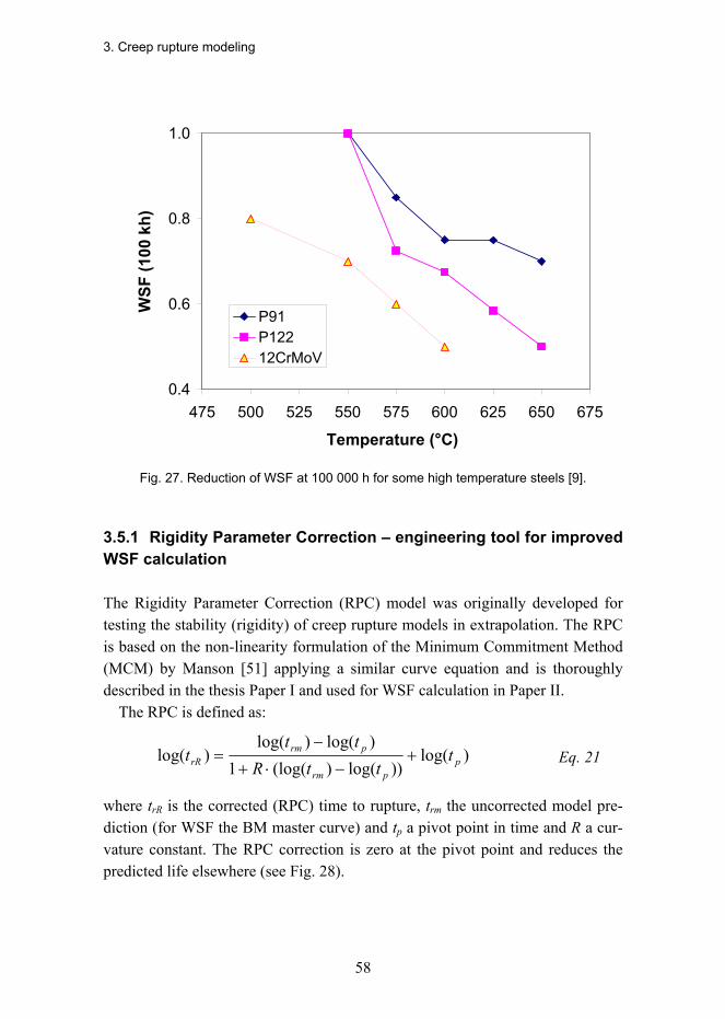
3. Creep rupture modeling
58
0.4
0.6
0.8
1.0
475 500 525 550 575 600 625 650 675
Temperature (°C)
WSF
(100
kh)
P91P12212CrMoV
Fig. 27. Reduction of WSF at 100 000 h for some high temperature steels [9].
3.5.1 Rigidity Parameter Correction engineering tool for improved WSF calculation
The Rigidity Parameter Correction (RPC) model was originally developed for testing the stability (rigidity) of creep rupture models in extrapolation. The RPC is based on the non-linearity formulation of the Minimum Commitment Method (MCM) by Manson [51] applying a similar curve equation and is thoroughly described in the thesis Paper I and used for WSF calculation in Paper II.
The RPC is defined as:
)log())log()(log(1
)log()log()log( p
prm
prmrR t
ttRtt
t +−⋅+
−= Eq. 21
where trR is the corrected (RPC) time to rupture, trm the uncorrected model pre-diction (for WSF the BM master curve) and tp a pivot point in time and R a cur-vature constant. The RPC correction is zero at the pivot point and reduces the predicted life elsewhere (see Fig. 28).
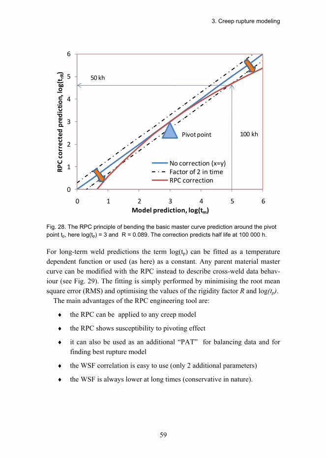
3. Creep rupture modeling
59
0
1
2
3
4
5
6
0 1 2 3 4 5 6
RPC corrected pred
ictio
n, log(t rR)
Model prediction, log(tm)
No correction (x=y)Factor of 2 in timeRPC correction
Pivot point 100 kh
50 kh
Fig. 28. The RPC principle of bending the basic master curve prediction around the pivot point tp, here log(tp) = 3 and R = 0.089. The correction predicts half life at 100 000 h.
For long-term weld predictions the term log(tp) can be fitted as a temperature dependent function or used (as here) as a constant. Any parent material master curve can be modified with the RPC instead to describe cross-weld data behav-iour (see Fig. 29). The fitting is simply performed by minimising the root mean square error (RMS) and optimising the values of the rigidity factor R and log(tp).
The main advantages of the RPC engineering tool are:
♦ the RPC can be applied to any creep model
♦ the RPC shows susceptibility to pivoting effect
♦ it can also be used as an additional PAT for balancing data and for finding best rupture model
♦ the WSF correlation is easy to use (only 2 additional parameters)
♦ the WSF is always lower at long times (conservative in nature).

3. Creep rupture modeling
60
10
100
2 2.5 3 3.5 4 4.5 5
Stress (M
Pa)
Time to rupture, log(h)
DataRPC predictionBMWSF=0.8
300
Fig. 29. Example of RPC modeling for cross-welded P91 data at 650°C, BM = base material.
0.4
0.5
0.6
0.7
0.8
0.9
1
2 2.5 3 3.5 4 4.5 5
WSF
Time to rupture, log(h)
RPC ‐ 650°C
RPC ‐ 625°C
RPC ‐ 600°C
RPC ‐ 575°C
Fig. 30. WSF for P91 steel using the RPC approach [Paper II].

3. Creep rupture modeling
61
3.5.2 Sensitivity analysis of P91 steel weld strength factor
To be able to check the sensitivity of the WSF, a set of cross-welded P91 steel data (ECCC data) was assessed by using the Wilshire equation (see section Creep rupture models for ferritic steels) using the RPC. The sensitivity of the WSF to changes in time to rupture was analyzed by random additions (or sub-traction) of continuously distributed time constants leading to additional data scatter. The maximum time change was limited to a factor of two for each (base material) rupture point of the NIMS data set used. The changes affected the mas-ter curve directly influencing the corresponding weld strength values (through the RPC). The calculated WSF effects on the simulated strengths are presented in Table 13.
The predicted time to rupture values for the cross welds using this concept are presented in Fig. 31.
100
1000
10000
100000
100 1000 10000 100000
Observed rupture time (h)
Pre
dict
ed ti
me
to ru
ptur
e (h
)
Fig. 31. Observed versus predicted time to rupture for P91 steel welds (XW) by using Wilshire equation for parent material (see Figs. 36) and RPC fitting for describing the XW ruptures. The data scatter factor for the weld data is 4.4.

3. Creep rupture modeling
62
Table 13. Monte-Carlo simulated (1000 simulations) WSF for rupture in 100 000 h for P91 steel with random changes in base material time to rupture.
Statistic 575ºC 600ºC
Max. 0.646 0.546
Min. 0.612 0.509
Mean 0.629 0.528 Std. Dev. 0.055 0.058
The WSF values calculated here are somewhat larger than those predicted for 100 000 h / 600ºC in the thesis Paper II, namely 0.48. The discrepancy is related to chosen base material master curve and the base material data used. In Paper II, the base material master curve was fitted to the standard 10, 100 and 250 kh rupture tables in the full temperature range described by the standard. To check for sensitivity to changes in the parameters R and log(tp) 10 000 random simula-tions were performed with ±10% variation to the parameters (triangular distribu-tions). The results are presented in Table 14.
Table 14. Monte-Carlo simulated (1000 simulations) WSF for random changes in the R (10%) and log(tp) (10%) parameter at 600°C / 100 000 h for P91 steel.
Statistic ∆R = ± 10% ∆ log(tp) ± 10%
Max. 0.573 0.565
Min. 0.483 0.505
Mean 0.527 0.531 Std. Dev. 0.026 0.018
The results indicate that the standard deviations for the predicted WSF are smaller than for the case with induced time scatter. It could be claimed that the model indeed produces robust WSF predictions.

4. Creep strain modeling
63
4. Creep strain modeling Creep strain sets design limits for many components in power engineering, such as for blading, bolts and casings of steam and gas turbines. In addition, creep strain is also an important quantity to be followed for the fit-for-service inspec-tions and follow ups of critical power plant components. The typical recom-mended limits range up to 12% of strain. However, measuring local strain and predicting it, in critical locations is not a simple task. The on-line monitoring equipments have today evolved to perform well, for instance, in the measure-ment of thick-walled high temperature components, but they are expensive and are of course not standard equipment in new installations. Also, the challenge would be to know where the most critical locations are.
From the FEA point of view the main contributor that creep modeling is not done very frequently is the short supply of relevant creep data and/or parameters for existing (implemented) creep routines. In comparison to creep rupture data, there is much less creep strain data available (especially in the public domain). Even for the commonly well established engineering steels such as P22 (10CrMo9-10) there is very few sources of creep strain data to be found.
Even today creep strain based remaining life assessments are based on mini-mum creep rate by Norton and the Monkman-Grant relationship. In work by Evans [77], the degree of uncertainty of the Monkman-Grant relationship has shown to be significantly underestimated. The simple minimum strain rate based models do not take the primary and tertiary creep regimes into account and therefore predict considerably lower strains.
The more advanced models usually need large creep-strain data sets to opti-mize a large number of material parameters. Some models have up to a total of 26 fitting constants [78] for defining the strain response in the defined stress and temperature range! Some strain models are quite established, such as the Ω-method [79] and the 4θ-method [80]. In the ECCC project Advanced creep a

4. Creep strain modeling
64
round robin was performed analyzing model equations in common use for creep deformation together with new approaches presented by the participating organi-zations (see Table 16). The assessors involved were from several international research and industrial organizations. In this context VTT presented a parametric strain model based on the Manson-Haferd and Grounes (Paper III of this thesis). The model was by far the simplest and also the one giving the best results in the whole range of strain predictions. The materials assessed by VTT were the P22 and P91 steels. The data sets represented single (P22) and multi cast data (P91), with continuous and interrupted creep strain measurements. The models were evaluated and reviewed for their effectiveness for various materials and practical applications.
The round robin recognized 3 approaches that defined all the models assessed:
1) Modeling individual creep curves and establishing curve model parame-ters ⇒ determination of stress and temperature dependence of these model parameters (examples: Mod. theta, Mod. Omega, BJF and Li-Akulov)
2) Producing synthetic data from the raw data in certain coordinates ε(T,σ, t) ⇒ parametric model fitting to synthetic data (examples: MHG and the modified Sandström model)
3) Producing synthetic data σ(T, ε, t) from ε(T,σ, t) raw data ⇒ model fitting to synthetic data (examples: Mod. Graham-Walles and Bolton)
In addition to this the new strain model presented in this thesis (see thesis Paper II), the logistic creep strain prediction (LCSP) adds a new approach to this list.
4) Fitting shape functions to strain curves or tabled stress to specific strain/time values with the true time to rupture value as end point ⇒ model complete when combing shape functions and time to rupture model.
From these the approaches the 2 and 3 were producing the best fit for both P22 single heat data and the P91 multi cast strain data sets (see Table 16 and

4. Creep strain modeling
65
Table 17). Note that the LCSP was not available at the time so it has been added to the end of the tables for comparison. The outcome of the round robin was used as platform for the ECCC recommendations and guidance for the assess-ment of creep strain and creep strength data (ECCC recommendations, Vol. 5 Part Ib). The recommendations include a review and references of the strain models listed in Table 15.
Table 15. Review of the ECCC round robin strain models [9].

4. Creep strain modeling
66
Table 16. Scatter factors Z for the ECCC round robin strain models for steel P22 (single heat data). P/S/T = primary / secondary / tertiary. In brackets the number of free parame-ters in the model.
Z for time to specified strain (all temperatures) Model equation
Creep re-gimes
0.2% 0.5% 1% 2% 5%
Omega model S/T (8) 468 39 10 - -
BJF model P/S 15 6 4 - -
Theta model P/S/T 17 3 2 - -
Modified Theta model
P/S/T 10 - 4 - -
Creep strength ratio model
P/S/T 4 8 7 - -
NPL model P/S/T 12 7 3 - -
Baker-Cane model P/S/T 5 2 - -
Bartsch model P/S 3 2 4 - -
Modified Garofalo P/S/T (28) 2 2 2 - -
Mod. Graham-Walles
P/S/T 3 3 2 2 2
Mod. Nadai P/S/T (11) 3 2 2 2 2
MHG-4 P/S/T (4) 3 3 3 3 3
LCSP P/S/T(81) 3 2 2 2 2 1) The tr(T,σ) parameters are not accounted for. Note that this model was not available at the time
of the round robin.

4. Creep strain modeling
67
Table 17. Calculated scatter factors Z for the assessed strain models for P91 steel (multi heat data set); P/S/T = primary / secondary / tertiary.
Z for time to specified strain (all temperatures) Model equation
Creep re-gimes
0.2% 0.5% 1 % 2% 5%
BJF model P/S 113 104 50 32 11
Modified Theta model
P/S/T 74 19 17 8 12
Li & Akulov P/S/T 143 42 18 6 4
Modified Omega S/T 138 19 11 8 5
Creep strength ratio model
P/S 38 7 7 6 5
Modified Sand-ström
P/S/T 11 7 6 6 6
Mod. Graham-Walles
P/S/T 7 7 6 7 5
MHG P/S/T 6 7 6 6 5
4.1 Manson-Haferd-Grounes (MHG) strain model engineering tool for creep strain prediction
The Manson-Haferd-Grounes model (MHG) is defined in depth in [81]. The main features are the simple method of predicting time to specific creep strain by assuming a parametric relationship (here Manson-Haferd) and that the creep mechanism remains the same following an Arrhenius type of temperature behav-ior. In addition it is assumed that the microstructural change (creep damage) can be related to the accumulated strain.
The MHG parameter is defined as:
MHG = [ln(tε)-C]/T = F(T,σ,ε), Eq. 22
where C is a constant, tε is the time to strain and F(T,σ,ε) is a multi-linear com-bination of temperature T, stress σ and strain ε.

4. Creep strain modeling
68
The MHG has mainly been tested for linear combinations of the following form:
[ln(tε)-C]/T = a0+a1·ln(σ)x+a2·ln(ε)y , Eq. 23 where a0, a1, a2, x and y are fitting constants. The x and y are low non-negative integers. The MHG parameters for P91 and P22 steels are given in Table 18. The MHG strain model for P22 steel is shown in Fig. 32.
Table 18. MHG strain functions for P22 and P91 steel.
Material Fitting constants
P22 [ln(tε)-55.62]/T = -33.2-0.95·ln(σ)2-0.2·ln(ε)2
P91 [ln(tε)-77.25]/T = -54.064-1.048·ln(σ)2-0.0294·ln(ε)3
The results suggest that the MHG model performs well and is robust with mini-mal number of fitting constants. The approach is theoretically applicable with both constant stress and constant load creep tests. Although the MHG model performed better than many of the other complex models (Table 16 and 17), some room for further improvement is possible, as is seen from the apparent systematic S-shaped trend in the PAT2 type prediction effectiveness plot for the multicast P91 data set (see Fig. 33).
4.74.8 4.9 5 5.1 5.2
5.3 5.4 5.55.6
ln(stress)-7-6
-5-4
-3-2
-1
ln(strain)
-75
-75
-70
-70
-65
-65
-60
-60
-55
-55
MH
G-4
* 1
000
MH
G-4
* 1
000
Fig. 32. Fitted MHG-4 master curve surface for P22 steel (single heat data).

4. Creep strain modeling
69
-2
-1
0
1
2
3
4
5
-2 -1 0 1 2 3 4 5
Measured log(time) to given strain
Pred
icte
d lo
g(tim
e) to
giv
en s
train
datata=tp·Zta=tpta=tp/Z
Z= 6.35
Fig. 33. PAT2 presentation for time to strain (MHG fitted) for multi heat P91 steel data.
The main observation from working with the parametric creep strain model MHG was that the parametric approach works surprisingly well but it could be further improved by a relationship to the curve end point (time to rupture). This observation was in fact the starting point of the development for the rupture based creep strain model LCSP described below.
4.2 Logistic Creep Strain Prediction (LCSP) engineering tool for robust creep strain prediction
The logistic creep strain prediction (LCSP) model is a creep strain prediction tool able to predict representative creep strain curves and strain rates in a large stress and temperature range. The limits of the stress/temperature are set by the available creep rupture data for the material in question. This is made possible with the help of actual (fitted to existing strain data) or assumed shape func-tions together with the time to rupture prediction. The best result in time to strain or strain at specified time is of course attained using the actual (true) rupture

4. Creep strain modeling
70
time of the individual creep curve. In extrapolation, or when data is missing the true rupture time is replaced by the master curve prediction for rupture.
The LCSP can be regarded as a further development of the MHG parametric models. The TTP based strain models were giving good fits and the incorpora-tion of the end points, namely the rupture time gives an advantage in compari-son to many other equations. The method introduces a transition in a temperature compensated time parameter (PLM) as a function of creep strain at specified tem-perature and stress. The PLM parameter calculated with time to strain instead of time to rupture changes as the strain accumulates from a parametric value of zero (small strain, short time) to a maximum value restricted by the rupture life and the LCSP parameter C (related to the Larson-Miller parameter C).
The LCSP function chosen for time to specified strain was the non-linear asymmetric transition function with a steepness regulated by two variables (p and x0, see Eq. 24). The reason for choosing this specific transition equation was due to its simple inverted form giving an algebraic solution for strain as a func-tion of time (Eq. 25). This inverted form was again easy to differentiate to give strain rate at a specified time. Further differentiation and finding the root of the expression gave the minimum creep rate. The LCSP equations for time to strain tε, strain at time εt and strain rate at speci-fied time )( εε t! are:
,))log((1
)log()log(
0
C
x
Ctt
p
r −+
+=
εε
Eq. 24
,1)log()log(
)log( 0
/1
xCtCt
pr
t ⋅⎟⎟⎠
⎞⎜⎜⎝
⎛−
++
=ε
ε Eq. 25
021 xkk ⋅⋅⋅−= εε! , Eq. 26
where tr is the time to rupture and x0, p and C are fitting factors. In its simplest form the last three are constants. The factors k1 and k2 are functions of time to strain. For the material models presented in this thesis the factors x0 and p are in all cases temperature and stress dependent multi-linear functions of the form:
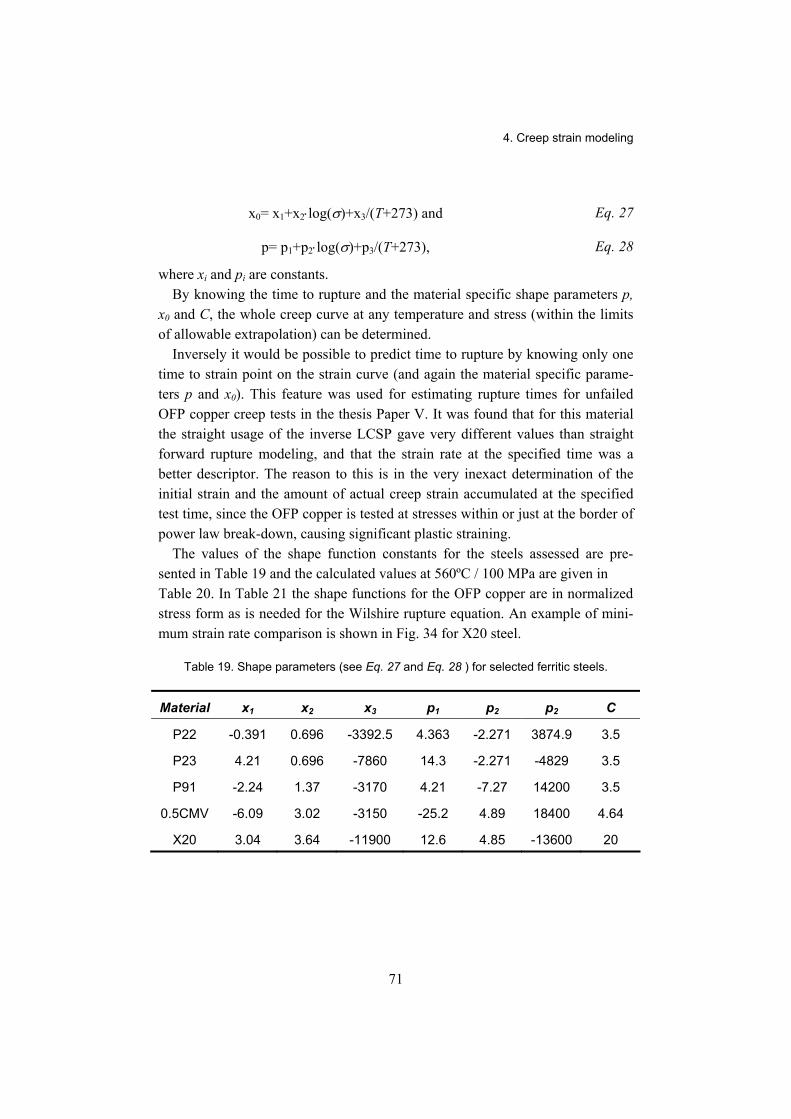
4. Creep strain modeling
71
x0= x1+x2⋅log(σ)+x3/(T+273) and Eq. 27
p= p1+p2⋅log(σ)+p3/(T+273), Eq. 28
where xi and pi are constants. By knowing the time to rupture and the material specific shape parameters p,
x0 and C, the whole creep curve at any temperature and stress (within the limits of allowable extrapolation) can be determined.
Inversely it would be possible to predict time to rupture by knowing only one time to strain point on the strain curve (and again the material specific parame-ters p and x0). This feature was used for estimating rupture times for unfailed OFP copper creep tests in the thesis Paper V. It was found that for this material the straight usage of the inverse LCSP gave very different values than straight forward rupture modeling, and that the strain rate at the specified time was a better descriptor. The reason to this is in the very inexact determination of the initial strain and the amount of actual creep strain accumulated at the specified test time, since the OFP copper is tested at stresses within or just at the border of power law break-down, causing significant plastic straining.
The values of the shape function constants for the steels assessed are pre-sented in Table 19 and the calculated values at 560ºC / 100 MPa are given in Table 20. In Table 21 the shape functions for the OFP copper are in normalized stress form as is needed for the Wilshire rupture equation. An example of mini-mum strain rate comparison is shown in Fig. 34 for X20 steel.
Table 19. Shape parameters (see Eq. 27 and Eq. 28 ) for selected ferritic steels.
Material x1 x2 x3 p1 p2 p2 C
P22 -0.391 0.696 -3392.5 4.363 -2.271 3874.9 3.5
P23 4.21 0.696 -7860 14.3 -2.271 -4829 3.5
P91 -2.24 1.37 -3170 4.21 -7.27 14200 3.5
0.5CMV -6.09 3.02 -3150 -25.2 4.89 18400 4.64
X20 3.04 3.64 -11900 12.6 4.85 -13600 20

4. Creep strain modeling
72
Table 20. Calculated shape parameters at 560ºC / 100 MPa.
Material x0(560,100) p(560,100) C
P22 -3.072 4.473 3.5
P23 -3.834 3.961 3.5
P91 -3.306 6.717 3.5
0.5CMV -3.832 6.669 4.64
X20 -3.966 5.973 20
Table 21. Shape functions x0 and p for OFP copper (σ in MPa, T in °C), C=3.5.
Shape function factors for OFP copper
x0(σ/σTS, T) = -2.179 + 4.397⋅ln(σ/σTS) - 0.008⋅T
p(σ/σTS, T) = 7.235 + 0.460⋅(σ/σTS)/ln(σ/σTS) - 0.012⋅T
1.0E-08
1.0E-07
1.0E-06
1.0E-05
1.0E-04
1.0E-08 1.0E-07 1.0E-06 1.0E-05 1.0E-04
Measured strain rate (1/h)
Pred
icte
d st
rain
rate
(1/h
)
Fig. 34. LCSP predicted minimum creep rates for X20 (12CrMoV 11-1) steel against measured creep rates.

5. Multi-axial creep strain and damage
73
5. Multi-axial creep strain and damage Structures operating in the creep regime will consume their creep life at a greater rate in locations where triaxiality constraint is unfavorable. Many structures develop different multi-axial stress states during creep related to their shape and dimensions. In addition discontinuities such as welds introduce multiple material zones with differing microstructures and material properties. These are also the locations where creep damage is found in service.
The solution of complex creep problems requires a method for handling multi-axial stresses and strains. The classical approach for describing the multi-axial stress state has been the von Mises yield criterion and its associated flow rule. It was, however, shown in the 60s [82] that the von Mises criterion underestimated creep for some cases in comparison to available data. This was corrected by introducing the general model of correlating damage under uniaxial tension with damage under more complex conditions by adopting an equivalent stress. There-fore, most early works on multi-axial long-term strength assessments are based on the equivalent stress. The equivalent stress concept is governed either by the maximum principal stress or by the von Mises effective stress. Generally it has been assumed that (macroscopically) the Von Mises effective stress controls creep deformation while maximum principal stress governs creep void formation (creep damage). Several other (mixed) components of stress have been proposed to describe the multiaxial rupture criterion [83], [84].
For structural integrity assessments, the calibration of the multi-axial material models has to be in place. This means that the multi-axial creep stress rupture criterion and/or the multi-axial creep ductility should be determined. For this purpose the notched-bar test programs [85] or maximum constraint testing (us-ing compact tension specimens) is valuable. The best tests to gain confidence in the established models are naturally large scale component tests successfully modeled without any model calibration.

5. Multi-axial creep strain and damage
74
The influence of creep life and ductility exhaustion under multi-axial condi-tions are implemented in some design codes [86], [87] but the implementation for life management and remaining life predictions of service exposed compo-nents is not yet satisfactorily solved. The work done with the FEA strain model implementation together with the multi-axial strain exhaustion filter described below is a sincere attempt to change this.
5.1 Engineering tool multi-axial LCSP for FEA
The creep strain rate formulation is based on the logistic creep strain prediction (LCSP) model implemented to ABAQUS, including primary, secondary and tertiary creep.
5.1.1 The FEA COMSOL implementation
For the COMSOL FE implementation the multi-axial LCSP creep strain rate expression has been attained from Eq. 26 by using a von Mises type flow rule and by deriving the expression for multi-axial creep strain rate (strain rate ten-sor) as follows:
),23)(()( 321 ijuij sTf ⋅++⋅= αβδαδαεε!
Eq. 29
where the first f(εu) is a function of the uniaxial LCSP model, δ, αi are constants, β(T) a function of temperature and sij is the deviatoric stress tensor.
The FE implementation itself is formulated using a mixed FE approach for the strain rate and solution of the balance equations using the weighted Galerkin method. The FE equations are interpolated adaptively varying the order of poly-nomic interpolation basis from 2 to 5. Time integration of the rate equations is carried out using an implicit back differentiation routine, with variable step-size and order.
The first versions of the LCSP implementation were used for determining creep damage in a simple girth welded pipe in the thesis Paper VI. Today the model implementation has been upgraded considerably and can now be used in more demanding case studies such as creep damage accumulation at defects and creep crack initiation predictions for compact tension (CT) specimen. In Fig. 35 a friction stir weld (FSW) test specimen (∅ 8 mm) with a weld root defect has

5. Multi-axial creep strain and damage
75
been simulated. The creep lives of the specimens taken from actual FSW welds are heavily reduced [18] in comparison to welds taken as cross-weld samples.
Fig. 35. Stress and strain state after 16 000 h of simulated creep testing (LCSP model) at nominal stress 80 MPa and 175ºC for a friction stir welded OFP copper creep specimen with a centrally located root defect.
5.1.2 The FEA ABAQUS implementation
For the ABAQUS implementation the LCSP model was implemented in its strain rate form, utilizing the CREEP user subroutine [88] and the Euler back-ward algorithm. The implementation is defined closer in the thesis Paper VII.
5.2 Engineering tool multi-axial exhaustion parameter
It is commonly known that for long-term creep of pressure vessels the maximum equivalent stresses and strains develop on the inner vessel surface whereas the maximum principal stress will redistribute towards the outer surface due to creep. The multi-axial creep ductility (due to the triaxiality constraint) will re-duce towards the outer surface as creep proceeds under long-term service. To be able to visualize this, a technique for filtering the acquired FE strains and stresses has been developed. The expression for rigid plastic deformation was used as a basis for the Λ-filtering technique (see Eq. 30 and Eq. 31). The equa-tions and their background are defined in the thesis Paper VII.
The Λ-filter is defined as:

5. Multi-axial creep strain and damage
76
εεεε
⋅=⋅−⋅
=Λfm
fu
h)5.1exp(65.1
⎥⎦
⎤⎢⎣
⎡⋅
=q
h kk
3σ ,
Eq. 30
Eq. 31
where kkσ is the trace of a stress tensor ijσ , ε the accumulated strain (maximum principal or von Mises), εfu and εfm the multiaxial and uniaxial creep ductility, respectively.
The main benefit of the filtering technique is that it does not require local creep ductility values. The Λ parameter is expressed as a ratio dependent on stress and momentary strain only, thus, making the strain exhaustion a ductility dependent quantity. The same basic concept is going to be used for further planned develop-ment of the strain exhaustion parameter. An example of a Λ-filtered FEA result (3D) for a repair welded P22 steam mixer is shown in Fig. 36.
The weld repair was performed after 100 000 h in service to lengthen the life of the creep damaged component. The full assessment is presented in [20].

5. Multi-axial creep strain and damage
77
4
2
1
3
4
2
1
3
Fig. 36. Overlay weld repair and simulated continued service for additional 100 000 h service for a creep damaged P22 steam mixer nozzle. The marked arrows point to (1) location of creep cracking, (2) predicted new location of damage, (3) secondary potential damage location at inner HAZ and (4) location of maximum creep strain. SDV1 = Λ-filter.

6. Discussion
78
6. Discussion The models and methodologies presented give a rather complete set of tools for assessing the creep rupture and/or creep strain data sets. The tools have been verified for a number of ferritic steels and the OFP copper for nuclear waste disposal canisters.
The MHG strain formulation was the first successful attempt of describing the strain response by a TTP parameter. The excellent fitting accuracy acquired from simple TTP strain relation was unexpected. The further refinement of the TTP based strain models finally lead to the current form of the LCSP model. The rupture based strain model has the benefit of utilizing the robustness ac-quired in the rupture model to be transferred into the strain model. The fitting accuracy to the strain data has not been compromised in the cases where both MHG and LCSP have been tested.
The LCSP is well suited also for producing parameters for other models as well. For instance the Norton law parameters are easily extracted from the full predicted creep curves by localizing the time of minimum strain rate at varying stresses and temperatures (Fig. 36). It is to be seen that the stress parameter n is both stress and temperature dependent and the classically temperature dependent parameter A(T), here presented in logarithmic form logA(T), is in fact also clearly stress dependent. The activation energy Qc, calculated both from mini-mum strain rate and rupture time, shows a very similar stress and temperature dependence as the Norton stress parameter (see Fig. 37).
The Omega method parameters widely used in the U.S [79], [89] are also easily extractable by linearization of the tertiary creep regime modeled with the LCSP.

6. Discussion
79
050
100150
Stress, MPa600
590580
570560
Temperature, °C
00
55
1010
1515
2020
2525
n - e
xpon
ent
n - e
xpon
ent
200
150
10050
Stress, MPa
600590580570560
Temperature, °C
-60-60
-50-50
-40-40
-30-30
-20-20
-10-10
log(
A[T
])
log(
A[T
])
Fig. 37. Norton stress exponent n and the temperature dependent parameter log(A[T]) calculated from LCSP minimum creep rates for P91 steel (550600ºC).
050
100150
Stress, MPa600
590580
570560
Temperature, °C
100100
300300
500500
700700
900900
11001100
Q (s
train
rate
), kJ
/mol
Q (s
train
rate
), kJ
/mol
0
50100
150Stress, MPa
600590
580570
560
Temperature, °C)
100100
300300
500500
700700
900900
11001100
Q (r
uptu
re),
kJ /m
ol
Q (r
uptu
re),
kJ /m
ol
Fig. 38. Activation energies calculated from a) minimum creep rates and b) rupture times for P91 steel (550600ºC).
The robustness of the LCSP as well as any rupture model attempted in this thesis is the result of extensive testing of the model, mainly comparing predicted versus true obtained values. The ECCC post assessment tests (PATs) together with the RPC engineering tool substantially lower the risk of ending up with an nonconservative model for rupture. Using the rupture time of a larger more equally distributed data set as basis (as the BM data usually is) instead of model-ing separate master curve for weldments improves the robustness of WSF calcu-lations. These tools optimally fitted and properly verified decrease the uncer-

6. Discussion
80
tainty of the extrapolated values. This will in turn lead to less premature damage in high temperature applications.
The models and tools presented are by no means complete and, for instance, the further development of the physical relationships to the shape curves of the LCSP should be attempted. Also, additional flexibility of the strain response fitting curves could be accomplished by temperature and perhaps even stress dependence for the C parameter. Maybe the p or x0 parameters could be turned into constants instead.
The LCSP applicability on the creep response of austenitic stainless steels should be investigated. A first step could be the SS 316 steel creep strain data assessed by ECCC.
The further assessment of OFP copper is also of great importance for the Fin-nish nuclear waste disposal scheme. The life predictions have been lowered at almost every step of data set updating or model refinement. The present life pre-dictions should be further refined when knowledge of creep ductility from long-term tests is available. Today the longest test duration for the OFP copper data at VTT has reached 70 000 h with over 20% of accumulated creep strain. The in-tergranular cracking detected on the specimen surface is somewhat alarming, since the phosphorus doping has been believed to remove the ductility and creep cracking problems of pure oxygen-free copper.
As already mentioned earlier, the multi-axial damage parameter needs further tuning to become more physically correct. The relationship of creep damage with maximum principal stress, hydrostatic stress and von Mises stress should be investigated further. However, the concept of using normalized strain exhaustion as a filter can be applied with improved versions of the Λ-filter.
The Wilshire model is a very promising rupture (and perhaps minimum creep rate) model. The best feature of this model is the low amount of modeling pa-rameters. Actually the only parameter that has to be determined is the apparent activation energy. Pre-determining the Qc* gives scatter factors higher than op-timal. The minimization of the scatter factor induces an offset to the linear func-tion describing the parameters u and k (Fig. 39). The activation energy used has though a significant impact on the long-term (thousands of years) predictions of the copper canister.

6. Discussion
81
y = 3.738x - 4.602R² = 0.968
-16
-14
-12
-10
-8
-6
-4
-2
0
-3.5 -2.5 -1.5 -0.5 0.5 1.5
ln(t r
exp
(Q/R
T))
ln(-ln(σ/σUTS))
DataOptimizedLinear (Data)
k=3.24u=1/1.18
Basic WEQ with Q=104 kJ/mol
Fig. 39. Wilshire parameter u and k determination for OFP copper using basic equation format and optimized values minimizing the scatter factor Z.

7. Conclusions
82
7. Conclusions Creep damage is unavoidably inflicted to materials stressed at high temperature, resulting in gradual strain accumulation and limited life. Suitable engineering tools are essential for satisfactory prediction of the creep performance in mate-rial development, design of components and structures, and life assessment of high temperature facilities.
In this thesis new tools have been described, tested and verified for accurate prediction of creep strain, damage and rupture for parent materials and welds of selected high temperature steels and OFP copper. The tools have been particu-larly designed aiming for reliability even when the background creep data sets are limited in size and scope.
The developed RPC and the LCSP methods can be used with the ECCC PATs to obtain robust creep strain and rupture models for parent materials and welds in the range of the test data up to the acceptable level of extrapolation. Compari-son within the ECCC suggests that the MHG and LCSP models for creep strain response are superior in performance to most if not all previous and more com-plex models, while only requiring a minimal number of fitting constants. Using a similar rule for predicted time to creep strain as for time to rupture, the allowable extrapolation could be for example extended by introducing lower bound LCSP simulated synthetic data into a PD 6605 assessment that can utilize unfailed data. This could be applied together with the current time in the running tests to obtain the maximum likelihood prediction of time to rupture. This approach needs to be further verified with data from long-term creep (strain) testing.
The fact that the LCSP model makes use of the background rupture models has clear advantages. This improves the experimental support for the model, as there are generally much more rupture data than creep strain data for any given material. The strain model is also simple and allows for straightforward expres-sions for strain, strain rate and life fractions. The model can define the strain

7. Conclusions
83
response with only three parameters (two stress and temperature dependent) in addition to those in the rupture models.
The new rupture and strain models have been implemented to finite element analysis (FEA) codes. The performance of the multi-axial version of the LCSP model appears superior to conventional Norton law based simulations. Case studies on steels and OFP copper have demonstrated the stability and usability of the implemented models. Simulations of girth welds in 10CrMo9-10 (P22) and X10CrMoVNb9-1 (P91) steels have shown that the LCSP model is working smoothly in COMSOL and ABAQUS FEA with acceptable calculation times. The introduced multi-axial creep exhaustion parameter (Λ) was shown to pin-point the realistic damage locations in welded high temperature components, although the concept may also benefit from further physical modeling of creep damage.
In conclusion, using the new tools with appropriate materials modeling and implementation of numerical analysis, the creep response can be evaluated for both uniaxial and multi-axial loading with benefits in both accuracy of the re-sults and efficiency in the analysis. Supporting creep data may be obtained from creep testing, materials standards and public domain sources. Ideally, relatively extensive data sets can be applied for this purpose, such as those from ECCC in Europe or NIMS in Japan. One of the main remaining sources of uncertainty is creep ductility, which is not well defined in most creep testing results.

8. Summary
84
8. Summary The work done in this thesis has provided new simple yet well performing tools to predict creep strain and life for material evaluation, component design and life as-sessment purposes. The uncertainty related to selecting the type of material model or determining weld strength factors has been reduced by the selection procedures and by linking the weld behavior to the base material master equation. Much of the re-sulting improvements and benefits are related to the reduced requirements for sup-porting creep data. The simplicity and robustness of the new tools also makes them easy to implement for both analytical and numerical solutions.
The thesis includes creep rupture and strain models for several ferritic steels for high temperature applications. The steels assessed are P22, P23, P24, 0.5CMV, X20, P91 and E911. Also, OFP copper with required extrapolation to very long service life has been assessed for the foreseen repository conditions of nuclear waste canisters. Furthermore, multi-axial creep damage behavior mod-eled with the new tools has been verified and visualized for a welded ex-service component.

85
References [1] Holmström, S. & Auerkari, P. Effect of short-term data on predicted creep rup-
ture life pivoting effect and optimised censoring. Materials at High Tempera-tures, Vol. 25 (2008), pp. 103109.
[2] Holmström, S. & Auerkari, P. Predicting weld creep strength reduction for 9% Cr steels. International Journal of Pressure Vessels Piping, Vol. 83 (2006), pp. 803808.
[3] Holdsworth, S. R., Askins, M., Baker, A., Gariboldi, E., Holmström, S., Klenk, A., Ringel, M., Merckling, G., Sandstrom, R., Schwienheer, M. & Spigarelli, S. Factors influencing creep model equation selection. International Journal of Pressure Vessels and Piping, Vol. 85 (2008) 12, pp. 8088.
[4] Holmström, S. & Auerkari, P. Robust prediction of full creep curves from mini-mal data and time to rupture model. Energy Materials, Materials Science & Engineering for Energy Systems, Vol. 1 (2006), pp. 249255.
[5] Holmström, S. & Auerkari, P. Predicting creep rupture from early strain data. Materials Science and Engineering: A, Vol. 510511 (2009), pp. 25−28.
[6] Holmström, S., Laukkanen A. & Calonius, K. Finding critical damage locations by Λ-filtering in FE modelling of a girth weld. Materials Science and Engineer-ing: A. Vol. 510511 (2009), pp. 224228.
[7] Holmström, S., Laukkanen, A., Rantala, J., Kolari, K., Keinänen, H. & Lehtinen, O. Modeling and verification of creep strain and exhaustion in a welded steam mixer. Journal of Pressure Vessel Technology, Vol. 131 (2009), 061405 (5 pages).
[8] EN 10216-2:2002+A2, 2007. Seamless steel tubes for pressure purposes - Technical delivery conditions - Part 2: Non-alloy and alloy steel tubes with specified elevated temperature properties.
[9] Abe, F., Kern, T.-U. & Viswanathan, R. (Eds). Creep-resistant steels. Abington Hall, Cambridge, England: Woodhead Publishing Ltd., March 2008. 700 p. ISBN 1 84569 178 4, ISBN-13: 978 1 84569 178 3.
[10] Kloos, K. H., Granacher, J. & Monsees, M. Creep equation for heat resistant steels. Steel Research, Vol 69 (1998), pp. 446453.

86
[11] Kloos, K. H., Granacher, J. & Monsees, M. Optimization and verification of creep equations for heat resistant steels. Steel Research, Vol. 69 (1998), pp. 454462.
[12] Holmström, S. & Auerkari P. Prediction of creep strain and creep strength of ferritic steels for power plant applications. International Conference on Life Management and Maintenance for Power Plants. HelsinkiStockholmHelsinki, 810 June 2004. Espoo: Technical Research Centre of Finland. VTT Symposium 234, Vol. 2, pp. 513521.
[13] Holmström, S., Laukkanen A. & Calonius, K. Visualising creep exhaustion in a P22 girth weld. International Conference on Life Management and Mainte-nance for Power Plants. HelsinkiStockholmHelsinki, 1214 June 2007. Espoo: Technical Research Centre of Finland. VTT Symposium 247, Vol. 2, pp. 208221.
[14] Holmström, S., Auerkari, P. & Holdsworth S. Predicting creep strain response from rupture data and robust creep curve model. International Conference on Life Management and Maintenance for Power Plants. HelsinkiStockholmHelsinki, 1214 June 2007. Espoo: Technical Research Centre of Finland. VTT Symposium 246, Vol. 1, pp. 185195.
[15] von Hartrott, P., Holmström, S., Caminada, S. & Pillot, S. Life time prediction for advanced low alloy steel P23. Materials Science and Engineering: A, Vol. 510511 (2009), pp. 175179.
[16] Rantala, J., Auerkari, P., Holmström S., Salonen J. & Laukkanen, A. Creep strain, damage and life prediction for welded 0.5CMV steel. 2nd International ECCC Conference. Creep & Fracture in High Temperature Components De-sign & Life Assessment. EMPA, Dübendorf, Switzerland, 2123 April 2009, pp. 669680.
[17] Auerkari, P., Holmström, S., Veivo. J. & Salonen J. Creep damage and ex-pected creep life for welded 911% Cr steels. International Journal of Pressure Vessels and Piping, Vol. 84 (2007), pp. 6974.
[18] Holmström, S., Auerkari, P. & Rantala, J. Engineering approach to creep strain modeling for multicast 9Cr steel. 11th Conference on Pressure Vessel Tech-nology, ASME PVP 2006/ICPVT-11. Vancouver, BC, Canada 2527 July 2006. American Society of Mechanical Engineers, ASME. 10 p.

87
[19] Auerkari, P., Holmström, S., Rantala, J. & Salonen, J. Creep damage, ductility and expected life for materials with defects. Proceedings of 2008 ASME Pres-sure Vessels and Piping Conference (PVP 2008). Chicago, Illinois, USA, 2731 July 2008. PVP2008-61428.
[20] Holmström, S., Rantala, J., Kolari, K., Keinänen, H., Laukkanen, A., Veivo, J. & Lehtinen, O. Life prediction for a weld repaired steam mixer. 2nd International ECCC Conference. Creep & Fracture in High Temperature Components De-sign & Life Assessment. EMPA, Dübendorf, Switzerland, 2123 April 2009, pp. 309319.
[21] Frost, H. J. & Ashby, M. F. Deformation Mechanism Maps. Oxford: Pergamon, 1982.
[22] Sandström, R., Andersson, H.C.M., Creep in phosphorus alloyed copper dur-ing power-law breakdown. Journal of Nuclear Materials, Vol. 372 (2008), pp. 7688.
[23] Wilshire, B. & Bache, M. B. Cost effective prediction of creep design data for power plant steels. Proceedings of the ECCC Creep Conference. Creep & Fracture in High Temperature Components - Design and Life Assessment Is-sues. Zürich, Switzerland, 2123 April 2009. Lancaster, Pa: DEStech Publica-tions, Inc, 2009. ISBN 978-1-60595-005-1.
[24] NIMS Atlas of creep deformation property No. D-1, Creep deformation proper-ties of 9Cr-1Mo-V-Nb steel tubes for boiler and heat exchangers, 2007.
[25] Evans, M. Critical review and appraisal of traditional and new procedures for the qualification of creep fracture behaviour using 1Cr-1Mo-0.25V steel. Journal of Engineering Materials and Technology, Vol. 131 (2009), 021011 (14 pages).
[26] EN 10291:2000. Metallic materials Uniaxial creep testing in tension Method of test.
[27] EN ISO 7500-2: 2000. Metallic materials. Verification of static uniaxial testing machines. Part 2: Tension creep testing machines. Verification and calibration of the force-measuring system.
[28] Granacher, J., Oehl, M. & Preussler, T. Comparison of interrupted and uninter-rupted creep rupture tests. Steel Research, issue No. 1/92 (1992), pp. 3945.

88
[29] EN 10216-2:2002+A2. Seamless steel tubes for pressure purposes Techni-cal delivery conditions Part 2: Non-alloy and alloy steel tubes with specified elevated temperature properties.
[30] Standard Data tables Vol. 2, Ferritic steels, SPRINT Specific project SPI-249, Implementation of Power Plant Component Life Assessment Technology Using a Knowledge-based system, 1995.
[31] Holdsworth, S. The European Creep Collaborative Committee (ECCC) ap-proach to creep data assessment. Journal of Pressure Vessel Technology, Vol. 130 (2008), 024001 (6 pages).
[32] von Hartrott, P. & Holmström, S. Lebensdauermodelle für den fortschrittlichen Stahl P23. 31. Vortragsveranstaltung der Arbeitsgemeinschaft für warmfäste Stähle und der Arbeitsgemeinschaft für Hochtemperaturwerkstoffe. 28 Nov. 2008. Düsseldorf, Germany: Stahlinstitut VDEh, 2008, pp. 2736.
[33] EN-SFS 10319-1:2003. Metallic materials. Tensile stress relaxation testing. Part 1: Procedure for testing machines.
[34] EN-SFS 10319-2:2006. Metallic materials. Tensile stress relaxation testing. Part 2: Procedure for bolted joint models.
[35] De Bruycker, E., Kaustermans, J-P. & Huysmans, S. Stress relaxation testing as an alternative to Conventional Creep Rupture testing. 2nd International ECCC Conference. Creep & Fracture in High Temperature Components De-sign & Life Assessment. EMPA, Dübendorf, Switzerland, 2123 April 2009.
[36] Steen M., Creep life assessment by low strain rate tensile testing. International Journal of Pressure Vessels and Piping Vol.14 (1983), Issue 4, pp. 201225.
[37] Penttilä, S., Toivonen, A., Heikinheimo, L. & Novotny, R. SCC properties and oxidation behaviour of austenitic alloys at supercritical water conditions. 4th In-ternational Symposium on Supercritical Water-Cooled Reactors. Heidelberg, Germany, 811 March 2009. 16 p.
[38] Sun, E., Hyde, T. H. & Brett, S. J. Application of impression creep data in life assessment of power plant materials at high temperatures. Proceedings of the Institution of Mechanical Engineers, Part L: Journal of Materials: Design and Applications, Vol. 222 (2008) 3, pp. 175182.

89
[39] Hyde, T. H., Sun, W. & Becker, A. A. Analysis of the impression creep test method using a rectangular indenter for determining the creep properties in welds. International Journal of Mechanical Sciences, Vol. 38 (1996) 10, pp. 10891102.
[40] Tu, S.-T., Segle, P. & Gong, J. M. Creep damage and fracture of weldments at high temperature. International Journal of Pressure Vessels and Piping, Vol. 81 (2004) 2, pp. 199209.
[41] Hyde, T. H., Yehia, K. A. & Becker, A. A. Interpretation of impression creep data using a reference stress approach. International Journal of Mechanical Sciences, Vol. 35 (1993) 6, pp. 451462.
[42] Blagoeva, D. T. & Hurst, R. C. Application of the CEN (European Committee for Standardization) small punch creep testing code of practice to a represen-tative repair welded P91 pipe. Materials Science and Engineering: A, Vol. 510511 (2009) June, pp. 219223.
[43] CEN Workshop Agreement, CWA 15627:2006 E, Small Punch Test Method for Metallic Materials. CEN, Brussels, Belgium, December 2006.
[44] Webster G. A., Holdsworth, S. R., Loveday, M. S., Nikbin, K., Perrin, I. J., Purper, H., Skelton, R. P. & Spindler, M. W. A Code of Practice for conducting notched bar creep tests and for interpreting the data. Fatigue & Fracture of Engineering Materials & Structures, Vol. 27 (2004) 4, pp. 319342.
[45] Besson, J., Leclercq, S., Gaffard, V. & Gourgues-Lorenzon, A.-F. Analysis of creep lifetime of a ASME Grade 91 welded pipe. Engineering Fracture Me-chanics (2009), Vol. 76, pp. 14601473.
[46] Holdsworth, S. R. & Merckling, G. ECCC developments in the assessment of creep-rupture data. In: Proceedings of Sixth International Charles Parsons Conference on Engineering Issues in Turbine Machinery, Power Plant and Re-newables. Trinity College, Dublin, 1618 September 2003.
[47] ECCC Recommendations. Creep data validation and assessment procedures. In: Holdsworth, S. R. et al. (Eds.) ECCC Publication (a) Vol. 1: Overview, (b) Vol. 2: Terms and terminology, (c) Vol. 3: Data acceptability criteria, data gen-eration, (d) Vol. 4: Data exchange and collation, (e) Vol. 5: Data assessment, (f) Vol. 6: characterisation of microstructure and physical damage for remaining
90
life assessment, (g) Vol. 7: Data assessment - creep crack initiation, (h) Vol. 8: Data assessment multi-axial, (i) Vol. 9: Component assessment.
[48] BS PD 6605. Guidance on methodology for assessment of stress-rupture data. London, UK: British Standard Institution, 1998.
[49] Fehér, A., Linn, S., Schwienheer, M., Scholz, A. & Berger, C. An interactive approach to creep behavior modeling. Materials Science and Engineering: A, Vol. 510511 (2009), June, pp. 2934.
[50] Goldhoff, R.M. Journal of Testing and Evaluation. Vol. 2 (1974), pp. 387424.
[51] Manson, S. S. & Ensign C. R.. Interpolation and extrapolation of creep rupture data by the minimum commitment method. Part I, Focal point convergence. Pressure Vessel & Piping Conference, Montreal (1978), pp. 299398.
[52] Trunin, I.I., Golubova, N.G. & Loginov, E.A. New method of the extrapolation of creep-test and long-time strength results. Proc 4th Int Symp on Heat-Resistant Metallic Materials, Mala Fatra, CSSR (1971), pp. 168176.
[53] Norton, F. N. The Creep of Steel at High Temperature. New York: McGraw-Hill, 1929.
[54] ECCC Data sheets, issue 2005. Creep rupture data sheet for E911 (X11CrMoWVNb9-1-1), assessed 2005. European Technology Development Publishers, 2005.
[55] ECCC Data sheets 2005. Creep rupture data sheet for P91 (X10CrMoVNb9-1), assessed 1995. European Technology Development Publishers, 2005
[56] ECCC Data sheets 2009. Creep rupture data sheet for P91 (X10CrMoVNb9-1) Released in the near future.
[57] Maruyama, K. & Yoshimi, K. Influence of data analysis method and allowable stress criterion on allowable stress of Gr.122 heat resistant steel. Trans ASME, Journal of pressure vessel technology, Vol. 129 (2007), pp. 449453.
[58] Kimura, K., Sawada, K. & Kushima, H. Influence of stress on creep deforma-tion properties of 912Cr ferritic creep resistant steels. 34th MPA-Seminar and VGB-Symposium Materials and Components Behaviour in Energy & Plant Technology, Stuttgart, 910 October 2008.
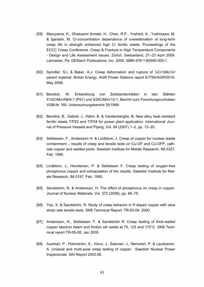
91
[59] Maruyama, K., Ghassemi Armaki, H., Chen, R.P., Yoshimi, K., Yoshizawa, M. & Igarashi, M. Cr-concentration dependence of overestimation of long-term creep life in strength enhanced high Cr ferritic steels. Proceedings of the ECCC Creep Conference. Creep & Fracture in High Temperature Components - Design and Life Assessment Issues. Zürich, Switzerland, 2123 April 2009. Lancaster, Pa: DEStech Publications, Inc, 2009. ISBN 978-1-60595-005-1.
[60] Spindler, S.L & Baker, A.J. Creep deformation and rupture of ½Cr½Mo¼V parent material. British Energy, AGR Power Stations report E/TSK/AGR/5516. May 2008.
[61] Bendick, W. Entwicklung von Zeitstandschäden in den Stählen X10CrMoVNb9-1 (P91) und X20CrMoV12-1, Bericht zum Forschungsvorhaben VGB-Nr 160. Untersuchungsbericht 35/1999.
[62] Bendick, B., Gabrel, J., Hahn, B. & Vandenberghe, B. New alloy heat resistant ferritic steels T/P23 and T/P24 for power plant application. International Jour-nal of Pressure Vessels and Piping, Vol. 84 (2007) 12, pp. 1320.
[63] Seitisleam, F., Andersson H. & Lindblom, J. Creep of copper for nuclear waste containment results of creep and tensile tests on Cu-OF and Cu-OFP, cath-ode copper and welded joints. Swedish Institute for Metals Research, IM-3327, Feb. 1996.
[64] Lindblom, J., Henderson, P. & Seitisleam F. Creep testing of oxygen-free phosphorus copper and extrapolation of the results. Swedish Institute for Met-als Research, IM-3197, Feb. 1995.
[65] Sandström, R. & Andersson, H. The effect of phosphorus on creep in copper. Journal of Nuclear Materials, Vol. 372 (2008), pp. 6675.
[66] Yao, X. & Sandström, R. Study of creep behavior in P-doped copper with slow strain rate tensile tests. SKB Technical Report, TR-00-09, 2000.
[67] Andersson, H., Seitisleam, F. & Sandström R. Creep testing of thick-walled copper electron beam and friction stir welds at 75, 125 and 175°C. SKB Tech-nical report TR-05-08, Jan 2005
[68] Auerkari, P., Holmström, S., Veivo, J., Salonen, J., Nenonen, P. & Laukkanen, A. Uniaxial and multi-axial creep testing of copper. Swedish Nuclear Power Inspectorate. SKI Report 2003:06.

92
[69] Auerkari, P., Holmström, S. & Salonen, J. Creep and creep damage in copper under uniaxial/multi-axial loading. Swedish Nuclear Power Inspectorate. SKI Report 2003:29.
[70] Auerkari, P., et al., Effects of defects on low temperature creep of OFP copper. 2nd International ECCC Conference. Creep & Fracture in High Temperature Components Design & Life Assessment. EMPA, Dübendorf, Switzerland, 2123 April 2009.
[71] Sandström, R. & Andersson, H.C.M. The effect of phosphorus on creep in copper. Journal of Nuclear Materials, Vol. 372 (2008) 1, pp. 6675.
[72] Raiko, H. Disposal canister for spent nuclear fuel design report. Posiva 2005-2, ISBN 951-652-134-7.
[73] Francis, J. A., Mazur, W. & Bhadeshia, H.K D.H. Type IV cracking in ferritic power plant steels. Materials Science and Technology, Vol. 22 (2006) 12, pp. 13871395.
[74] Wilshire, B. & Scharning, P. J. Creep ductilities of 912% chromium steels. Scripta Materialia, Vol. 56 (2007), pp. 10231026.
[75] Kimura, K., Kushima, H. & Sawada, K. Long-term creep deformation property of modified 9Cr1Mo steel. Materials Science and Engingeering: A, Vol. 510-511 (2009), June, pp. 5863. doi:10.1016/j.msea.2008.04. 095.
[76] Spindler, M. W. & Spindler, S. L. Creep deformation, rupture and ductility of Esshete 1250. International Journal of Pressure Vessels and Piping, Vol. 85 (2007) 12, pp. 8998. doi:10.1016/j.ijpvp.2007.06.004.
[77] Evans, M. Some interpolative properties of the Monkman-Grant empirical rela-tion in steel tubes. International Journal of Pressure Vessels and Piping, Vol. 72 (1997) 3, August, pp. 177191.
[78] Granacher, J., Möhlig, H., Schwienheer, M. & Berger, C. Creep equations for high temperature materials. Proceedings of Seventh International Conference on Creep and Fatigue at Elevated Temperatures (CREEP 7). NRIM, Tsukuba, 3-8 June 2001. Tokyo: The Japan Society of Mechanical Engineers, pp. 609616.

93
[79] Prager, M. Development of the MPC Omega method for life assessment in the creep range. ASME Journal of Pressure Vessel Technology, Vol. 117 (1995) May, pp. 95103.
[80] Evans, M. Combining predictions in a simplified 4Θ methodology for creep life assessment: an application to 2Cr-1Mo steel. Materials Science and Technol-ogy, Vol. 22 (2006) 2, pp. 173185.
[81] Holmström, S., Auerkari, P. & Holdsworth, S. An effective parametric strain model for creep. Materials for Advanced Power Engineering 2006. Proceed-ings of the 8th Liège Conference, part III. Forschungszentrum Jülich GmbH, pp. 13091318.
[82] Manson, S. S. Design considerations for long life at elevated temperatures (James Clayton Lecture). Proc. Institution of Mechanical Engineers, 19631964.
[83] Yao, H-T., Xuan, F-Z., Wang, Z., Tu, S-T. A review of creep analysis and de-sign under multi-axial stress states. Nuclear Engineering and Design, Vol. 237 (2007) pp. 19691986.
[84] Gorash, Y. Development of a creep-damage model for non-isothermal long-term strength analysis of high-temperature components operating in a wide stress range. Ph.D. Thesis. Zentrum für Ingenieurwissenschaften der Martin-Luther-Universität, Halle-Wittenberg, Germany, 21 July 2008. 106 p.
[85] Yatomi, M., Bettison, A. D., ODowd N. P. & Nikbin, K. M. Modelling of damage development and failure in notched-bar multi-axial creep tests. Fatigue & Frac-ture of Engineering Materials & Structures, Vol. 27 (2004) 4, pp. 283295.
[86] R5 (2001) Assessment procedure for the high temperature response of struc-tures. British Energy, Glouchester, UK.
[87] RCC-MR (1987), Design and construction rules for mechanical components of FBR nuclear islands, Paris, France.
[88] ABAQUS. ABAQUS Online Documentation: Version 6.7-1. Theory Manual [CD-ROM]. ABAQUS Inc., 2007.
[89] Prager, M., The Omega method: an engineering approach to life assessment. ASME Trans., Journal of Pressure Vessel Technology, Vol. 122 (2000), pp. 273280.

Error! No text of specified style in document.
1
Appendices II, III, V and VI of this publication are not included in the PDF version. Please order the printed version to get the complete publication (http://www.vtt.fi/publications/index.jsp).
94

Paper I
Effect of short-term data on predicted creep rupture life – pivoting effect and optimized
censoring
In: Materials at High Temperatures. Vol. 25 (2008) 3, September, pp. 103–109.
Northampton, UK: Science Reviews 2000 Ltd. Reprinted with permission from the publisher.


Black plate (103,1)
Effect of short-term data on predicted creep
rupture life – pivoting effect and optimized
censoring
S. Holmstrom and P. Auerkari
VTT, Espoo, Finland
ABSTRACT
Fitting data to classical creep rupture models can result in unrealistically high extrapolated long-term
strength. As a consequence, the standard strength values for new steel grades have frequently needed
downward correction after obtaining more long-term test data. The reasons for non-conservative
extrapolation include the influence of short-term data, which are easiest to produce but tend to pivot
upwards the extrapolated values of creep rupture strength. Improvement in extrapolation could be
expected by reducing this effect through model rigidity correction and censoring of very short-term
data, but it may not be immediately clear how to justify the correction of particular models or
censoring.
Analogously to the instability parameter in the minimum commitment model for creep rupture, a
rigidity parameter correction (RPC) is introduced to assess the pivoting effect of creep rupture models
for the purpose of reducing potential to non-conservativeness in extrapolation. The RPC approach can
be used with any creep rupture model for comparing the model rigidity and the potential benefit from
censoring short-term data. The correction itself will never introduce non-conservatism, regardless of
the model. The RPC approach is demonstrated by analyzing an ECCC data set for cross-welded 9%Cr
steel (E911).
Keywords: short-term data, creep rupture life, pivoting effect, optimized censoring
1. INTRODUCTION
The creep rupture data used for evaluating the representative
creep strength typically spans over several orders of magni-
tude in time. As relatively short-term tests are obviously
fastest and cheapest to perform, they are better represented
than long-term tests in the data sets. In addition, the damage
and failure mechanisms in the short-term tests tend to differ
from those in the long-term tests, which may better represent
the foreseen service conditions. Although the fitted creep
rupture models can accommodate much of the resulting
curvature in the creep rupture strength vs. time curves,
some residual curvature is not included. This has often
resulted in overestimated values of new material strength,
so that standard values had to be later reduced when
additional long-term data have become available. The
reasons for the overestimates can include long-term degrada-
tion and bias in material sampling, for example. However,
the common reasons can also include the pivoting effect by
‘‘over-represented’’ short-term tests, which may unduly
increase the extrapolated creep rupture strength (and life)
unless at least partially censored for fitting. This effect also
depends on the rigidity or the creep rupture model, or its
inherent ability to describe both the short and the long
duration data. The main interest in most cases is in extra-
polation towards long-term service conditions, and therefore
the effect of pivoting and data censoring are of interest for
extrapolation accuracy.
The rigidity parameter correction (RPC) method presented
here is a tool for quantifying the rigidity of creep rupture
models and the likely extrapolation error due to pivoting, and
for optimized data censoring. As an example, an ECCC data
set with cross-welded 9%Cr material (E911) data is analyzed
using RPC. First a series of models are compared for rigidity
and likely extrapolation error due to pivoting. For this data
set it is known that the fracture location is changing from
base material fractures to fractures in the heat affected zone
(HAZ), leading to a change in the curvature. Most creep
rupture models are expected to show pivoting problems with
such data sets. Finally, some data-censoring options are
tested for this data set.
2. METHODS, APPLIED MODELS AND TEST
DATA
The RPC approach applies a similar non-linearity formula-
tion as the master curve equation of the Manson’s [1]
minimum commitment method (MCM):
logðtr*Þ ¼GðsÞ PðT Þ
1þ A PðT Þð1Þ
MATERIALS AT HIGH TEMPERATURES 25(3) 103–109 103
0960-3409/3/2008# 2008 Science Reviews 2000 Ltddoi: 10.3184/096034008X354747
I/1
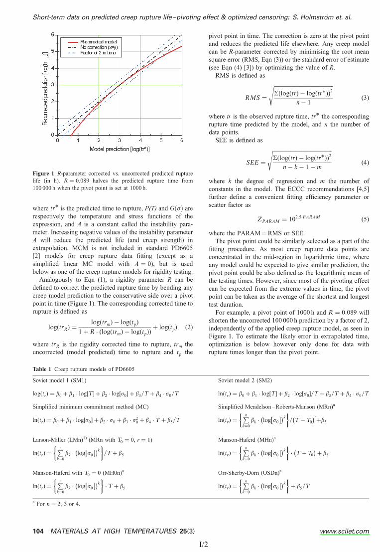
Black plate (104,1)
where tr* is the predicted time to rupture, P(T) and GðsÞ are
respectively the temperature and stress functions of the
expression, and A is a constant called the instability para-
meter. Increasing negative values of the instability parameter
A will reduce the predicted life (and creep strength) in
extrapolation. MCM is not included in standard PD6605
[2] models for creep rupture data fitting (except as a
simplified linear MC model with A ¼ 0), but is used
below as one of the creep rupture models for rigidity testing.
Analogously to Eqn (1), a rigidity parameter R can be
defined to correct the predicted rupture time by bending any
creep model prediction to the conservative side over a pivot
point in time (Figure 1). The corresponding corrected time to
rupture is defined as
logðtrRÞ ¼logðtrmÞ logðtpÞ
1þ R ðlogðtrmÞ logðtpÞÞþ logðtpÞ ð2Þ
where trR is the rigidity corrected time to rupture, trm the
uncorrected (model predicted) time to rupture and tp the
pivot point in time. The correction is zero at the pivot point
and reduces the predicted life elsewhere. Any creep model
can be R-parameter corrected by minimising the root mean
square error (RMS, Eqn (3)) or the standard error of estimate
(see Eqn (4) [3]) by optimizing the value of R.
RMS is defined as
RMS ¼
ffiffiffiffiffiffiffiffiffiffiffiffiffiffiffiffiffiffiffiffiffiffiffiffiffiffiffiffiffiffiffiffiffiffiffiffiffiffiffiffiffiffiffiSðlogðtrÞ logðtr*ÞÞ2
n 1
sð3Þ
where tr is the observed rupture time, tr* the corresponding
rupture time predicted by the model, and n the number of
data points.
SEE is defined as
SEE ¼
ffiffiffiffiffiffiffiffiffiffiffiffiffiffiffiffiffiffiffiffiffiffiffiffiffiffiffiffiffiffiffiffiffiffiffiffiffiffiffiffiffiffiffiSðlogðtrÞ logðtr*ÞÞ2
n k 1 m
sð4Þ
where k the degree of regression and m the number of
constants in the model. The ECCC recommendations [4,5]
further define a convenient fitting efficiency parameter or
scatter factor as
ZPARAM ¼ 102:5PARAMð5Þ
where the PARAM¼RMS or SEE.
The pivot point could be similarly selected as a part of the
fitting procedure. As most creep rupture data points are
concentrated in the mid-region in logarithmic time, where
any model could be expected to give similar prediction, the
pivot point could be also defined as the logarithmic mean of
the testing times. However, since most of the pivoting effect
can be expected from the extreme values in time, the pivot
point can be taken as the average of the shortest and longest
test duration.
For example, a pivot point of 1000 h and R ¼ 0:089 will
shorten the uncorrected 100 000 h prediction by a factor of 2,
independently of the applied creep rupture model, as seen in
Figure 1. To estimate the likely error in extrapolated time,
optimization is below however only done for data with
rupture times longer than the pivot point.
Short-term data on predicted creep rupture life–pivoting effect & optimized censoring: S. Holmstrom et. al.
104 MATERIALS AT HIGH TEMPERATURES 25(3) www.scilet.com
Figure 1 R-parameter corrected vs. uncorrected predicted rupture
life (in h). R ¼ 0:089 halves the predicted rupture time from
100 000 h when the pivot point is set at 1000 h.
Table 1 Creep rupture models of PD6605
Soviet model 1 (SM1) Soviet model 2 (SM2)
logðtrÞ ¼ b0 þ b1 log½T þ b2 log½s0 þ b3yT þ b4 s0yT lnðtrÞ ¼ b0 þ b1 log½T þ b2 log½s0yT þ b3yT þ b4 s0yT
Simplified minimum commitment method (MC) Simplified Mendelson –Roberts-Manson (MRn)a
lnðtrÞ ¼ b0 þ b1 log½s0 þ b2 s0 þ b3 s20 þ b4 T þ b5yT lnðtrÞ ¼
Pnk¼0
bk log s0
k y T T0
rþb5
Larson-Miller (LMn)1) (MRn with T0 ¼ 0, r ¼ 1) Manson-Haferd (MHn)a
lnðtrÞ ¼Pnk¼0
bk log s0
k yT þ b5 lnðtrÞ ¼
Pnk¼0
bk log s0
k T T0
þ b5
Manson-Haferd with T0 ¼ 0 (MH0n)a Orr-Sherby-Dorn (OSDn)a
lnðtrÞ ¼Pnk¼0
bk log s0
k T þ b5 lnðtrÞ ¼
Pnk¼0
bk log s0
k þ b5yT
a For n ¼ 2, 3 or 4.
I/2

Black plate (105,1)
In this work the non-linear MCM model was tested
together with a selection of PD6605 [2] creep rupture
models. The PD6605 supported models (18 model variants
in total, see Table 1) apply maximum likelihood linear fitting
to the rupture test data. An advantage of this approach is the
possibility of using unfailed data (ongoing or interrupted
tests) in the assessment.
Applying RPC for models selected by ECCC post assess-
ment testing (PAT) will further characterise their suitability
for extrapolation. A rigid model or a ‘‘difficult’’ data set
might require left censoring (in time) or stress censoring
(isothermal) for improved reliability. Optimizing R on data
with longer rupture times than the pivot point again quanti-
fies the likely error in the extrapolated life. A large positive
value of R would suggest a model (andyor data) susceptible
to pivoting errors, and non-conservative (uncorrected)
predicted life.
To show the potential of RPC, an ECCC data set of cross-
welded 9%Cr material (E911) is fitted to the selected creep
ruptured models. A series of models are compared for their
fitting efficiency with and without RPC, and then their likely
extrapolation error due to pivoting is quantified. Finally, data
censoring options are tested for potential improvement in
extrapolation. For this data set it is known that the fracture
location is changing from the base material to the heat
affected zone (HAZ). Such a data set can be expected to
show pivoting problems with most creep rupture models.
The full data set consists of 159 ruptured and 36 unfailed
data points including specimens ruptured in the parent
material, weld metal and in the heat affected zone (HAZ).
The data covers a temperature range of 550 – 690C and
stress range of 26 – 230 MPa, with the longest ruptured test
about 32 000 h and the longest unfailed test about 65 000 h in
duration. In addition to the full data set, subsets of data are
analyzed on HAZ failures without censoring and with left
censoring up to 1000 h. A source for error in the PD6605
models is possible when assessing HAZ data only; caused by
the fact that there are unfailed data in isotherms (550 and
575C) where there are no failed data. The impact of this
situation on the models should be clarified in future work.
3. COMPARISON OF CREEP MODELS WITH RPC
FOR CROSS-WELDED 9Cr STEEL
Nine best-fitting PD6605 models and the MCM model were
selected for RPC applied to the ECCC data set on cross-
welded 9Cr steel. The RPC optimization results on all data
are shown in Table 2, when the pivot point is set at 1000 h.
For all models it can be noted that the RPC reduces the
scatter factor ZSEE by 5 – 13%.
Rating the models according to the result of the RPC (the
smaller the R-parameter the better), the best (MCM and MC)
and worst (OSD2) performing models are compared with
uncorrected models in Figure 2.
For comparison, the same data set was RPC optimized on
data longer than the pivot point. The resulting values of R
and Z for the models before and after RPC are presented in
Table 3, and a comparison of uncorrected and corrected best
and worst performing models is shown in Figure 3. The time
ratio trRytrm at longest observed rupture time (about
30 000 h) and at 100 000 h are also listed to characterise the
effect of optimized RPC. Again, ZSEE is systematically
reduced by RPC but the reduction is now between 0.4 and
4.1%. The predicted life at 30 000 h (uncorrected) is reduced
by about 15 – 30% depending on model. Of the PD6605
models, the MC model showed smallest value of Z and R
(and largest time ratio), while OSD2 showed the largest Z
and R. The non-linear MCM gave no more obvious improve-
ment in this case in comparison with the simplified minimum
commitment model (MC).
Short-term data on predicted creep rupture life–pivoting effect & optimized censoring: S. Holmstrom et. al.
www.scilet.com MATERIALS AT HIGH TEMPERATURES 25(3) 105
Figure 2 RPC fits of the two best performing models (MCM, MC)
and the worst performing OSD model, with a pivot point at 1000 h.
Table 2 Calculated values of R and Z for selected creep rupture models, optimized on all data. The model scatter factors (both RMS andSEE Z-values) are presented before and after RPC. The pivot point is set to 1000 h
Model ZRMS ZSEE R-parameter(uncorrectedyR-corrected) (uncorrectedyR-corrected)
MC 4.95y4.68 5.11y4.87 0.095OSD3 4.90y4.27 5.03y4.42 0.165MH03 4.85y4.23 4.97y4.37 0.159MR03 5.16y4.47 5.30y4.62 0.181SM1 5.76y5.07 5.92y5.26 0.179SM2 5.75y5.04 5.91y5.23 0.182MR02 7.99y7.15 8.21y7.43 0.197MH02 9.23y8.26 9.49y8.61 0.185OSD2 9.07y7.96 9.34y8.29 0.219MCM (A¼ 0.155) 3.82y3.69 3.95y3.85 0.052
I/3

Black plate (106,1)
4. OPTIMAL CENSORING OF 9Cr CROSS-WELD
DATA USING RPC
Three cross-weld data subsets of the 9Cr material were tested
for optimal performance by left censoring. The first subset
included HAZ failures only, the second the same data set
censored up to 300 hours and the third subset the same data
set censored up to 1000 hours. In all cases the pivot point is
set at 3000 h (mid-range of data with HAZ failures).
4.1 HAZ failures, no censoring
With RPC, the predicted life is shortened by a factor of two
in time from 100 000 h with R ¼ 0:1618, when the pivot
point is set at 3000 h. The RPC optimization results with all
data are shown for the MC, MCM and the ODS2 models in
Table 4, and the corresponding results for data above pivot
point in Table 5.
The removal of data not failing in the HAZ changes the
order of the MC and OSD2 models indicating that the MC
behaves more rigidly for these data. However, the MCM
model hardly changes at all by RPC, in fact the ZSEE is
getting worse which indicate that the RPC does not represent
a true improvement for this model.
From the extrapolation point of view the two PD6605
models perform very similarly, and both MC and OSD2
models seem to suffer from the pivoting effect in extrapola-
tion. The MCM model again shows decline in the ZSEE
scatter factor by RPC. The MCM is thereby nearly optimal
without further correction, and would be selected as
preferred model for the HAZ failure data assuming it also
passes all PAT tests. However, again one has to remember
Short-term data on predicted creep rupture life–pivoting effect & optimized censoring: S. Holmstrom et. al.
106 MATERIALS AT HIGH TEMPERATURES 25(3) www.scilet.com
Table 3 Calculated values of R and Z for the same creep rupture models as in Table 2, optimized on all rupture data above the pivot point(1000 h). The scatter factors (Z) are shown with and without RPC. The models shown in bold are further applied to the data points ofHAZ failures
Model ZRMS ZSEE R Time ratio trRytrm at(uncorrectedyR-corrected) (uncorrectedyR-corrected) 30 000 hy100 000 h
MC 2.40y2.37 2.45y2.44 0.032 0.858y0.758OSD3 2.59y2.48 2.64y2.55 0.055 0.774y0.634MH03 2.60y2.49 2.65y2.56 0.057 0.768y0.624MR03 2.62y2.50 2.68y2.57 0.058 0.765y0.620SM1 2.93y2.83 3.0y2.91 0.057 0.768y0.624SM2 2.95y2.83 3.01y2.92 0.058 0.765y0.620MR02 3.46y3.34 3.54y3.45 0.061 0.755y0.606MH02 3.78y3.62 3.86y3.74 0.071 0.724y0.564OSD2 3.89y3.72 3.98y3.84 0.074 0.715y0.552MCM (A¼ 0.155) 2.48y2.42 2.56y2.51 0.045 0.809y0.684
Note that here the usually well behaving SM1 model appears to behave rigidly, giving inferior results in comparison with MC and MCM.
Figure 3 RPC fits of the best performing models (MC and MCM)
and the worst performing (OSD2) model. The models are optimized
on data above the pivot point (1000 h).
Table 4 Calculated values of R and Z for MC, OSD2 and the MCM models, fitted and RPC optimized on uncensored data of HAZ fail-ures (pivot point at 3000 h)
Model ZRMS ZSEE R(uncorrectedyR-corrected) (uncorrectedyR-corrected)
MC 2.20y2.09 2.26y2.16 0.166OSD2 2.21y2.11 2.25y2.17 0.145MCM (A¼ 0.13) 2.09y2.09 2.17y2.18 0.028
Table 5 Calculated values of R and Z for best and worst performing PD6605 models and MCM model on the full data set, optimized onHAZ data with longer durations than 3000 h (pivot point)
Model ZRMS ZSEE R Time ratio at time of(uncorrectedyR-corrected) (uncorrectedyR-corrected) 30 000 hy100 000 h
MC 2.22y2.12 2.31y2.23 0.134 0.762y0.552OSD2 2.26y2.16 2.32y2.24 0.133 0.763y0.554MCM (A¼ 0.13) 2.15y2.14 2.26y2.29 0.019 0.958y0.906
I/4

Black plate (107,1)
that the MCM model has not utilised the unfailed data and
might therefore show better fits.
4.2 HAZ failures, left censoring at 300 h
It is to be noted that the difference from the uncensored data
set is only one failed data point at 262 hours ðlogðtrÞ ¼ 2:4Þ;the next shortest test has a logarithmic rupture time of 2.8
(630 h). The RPC optimization results are shown here for the
MC and OSD2 models in Table 6 for the whole data range
and in Table 7 for the data above the pivot point. The
pivoting point is still kept at 3000 h.
The OSD2 model seems to behave more flexibly than the
MC model. From the extrapolation point of view the MC
model shows no change in the R-parameter as an effect of the
left censoring (in comparison to the uncensored HAZ data
set), indicating that the culling does not affect this model.
The OSD2 model shows some decrease in the value of R,
suggesting an improvement.
4.3 HAZ failures only, left censoring at 1000 h
The pivot point is still kept at 3000 hours for comparison
reasons and to avoid a too short bending range for the long-
term data. The RPC optimization is performed on the left
censored HAZ data using the same MC and OSD2 models as
before. The RPC results are presented in Table 8 for
optimized R-parameter on the whole range and in Table 9
on the data above the pivoting point.
From the rigidity point of view both the MC and the
OSD2 show only slight improvement in the R-parameter (in
comparison to the less culled and un-culled data sets). The
location of the pivoting point closer to the short duration end
(due to culling) emphasizes the long duration end, which can
be seen comparing Table 8 and Table 9 (which are nearly
identical). This indicates that any pivoting due to the shorter
test data (1000 to 3000 h) can be ruled out.
The OSD2 performs better the more left-censoring is
applied whereas the MC show no clear improvement in the
R-parameter. This suggests that the uncensored HAZ data is
already the optimal data set for MC to perform the assess-
ment, and that further censoring only favours relatively
simple models such as the OSD2.
5. DISCUSSION AND CONCLUSIVE REMARKS
The RPC approach is available to supplement any classical
creep rupture model, including those supported by
PD6605. RPC will typically reduce the common inherent
non-conservatism in predicted life, because it can justify
additional downward curvature to the (e.g. isothermal)
extrapolated creep rupture curves. As the correction is
zero at the selected pivot point and reduces life elsewhere,
RPC itself is not likely to be non-conservative. In the
example case of cross-welded 9Cr steel, the data fits were
improved by RPC (improvement in scatter factor) for all
tested PD6605 creep models, and in each case by addi-
tional curvature towards the non-conservative side. This
suggests good potential in reducing the commonly
observed non-conservatism in extrapolated creep rupture
life. In the example data set for cross-welded 9Cr steel,
the resulting reduction in predicted life was 15 – 25% at
30 000 h and 24 – 45% at 100 000 h for the tested models,
which corresponds to the maximum observed failure time
and maximum target extrapolation time.
For the full data set the MC and MCM models were least
affected by pivoting (see Figure 4). The relatively inflexible
SM1 and SM2 models require more correction, and should
be RPC tested when post assessment tests (PAT) suggest
these as preferred models.
Short-term data on predicted creep rupture life–pivoting effect & optimized censoring: S. Holmstrom et. al.
www.scilet.com MATERIALS AT HIGH TEMPERATURES 25(3) 107
Table 6 Calculated values of R and Z for best and worst perform-ing PD6605 models on all HAZ failure data, left censored at300 h
Model ZRMS ZSEE R(uncorrectedyR-corrected) (uncorrectedyR-corrected)
MC 2.19y2.09 2.25y2.17 0.152OSD2 2.20y2.12 2.24y2.18 0.135
Table 8 Calculated values of R and Z for best and worst perform-ing PD6605 models on the full HAZ data set, optimized on dataleft censored at 1000 h
Model ZRMS ZSEE R(uncorrectedyR-corrected) (uncorrectedyR-corrected)
MC 2.18y2.08 2.22y2.16 0.131OSD2 2.18y2.14 2.23y2.20 0.108
Table 7 Calculated values of R and Z for best and worst performing PD6605 models on HAZ failure data, left censored at 300 h andabove the pivot point
Model ZRMS ZSEE R Time ratio at max rupture time(uncorrectedyR-corrected) (uncorrectedyR-corrected) (30 000 hy100 000 h)
MC 2.22y2.11 2.31y2.22 0.134 0.762y0.552OSD2 2.24y2.15 2.30y2.24 0.125 0.774y0.571
Table 9 Values of R and Z as in Table 8 but for failures above the pivot point
Model ZRMS ZSEE R Time ratio at max rupture time(uncorrectedyR-corrected) (uncorrectedyR-corrected) (30 000 hy100 000 h)
MC 2.18y2.09 2.27y2.19 0.130 0.767y0.560OSD2 2.19y2.13 2.25y2.21 0.107 0.800y0.612
I/5

Black plate (108,1)
Looking at the improvement of fit above the
pivoting point (see Figure 5), it appears that the
RPC does not improve badly fitting models (in
expected time scatter) more than the initially better
ones.
Plotting the corrected and uncorrected models
(all data case, see Figure 6) it can be seen that for
this data set the 625C isotherm is improved the
most from the RPC.
For the subsets on HAZ failures it was shown
that left censoring does not improve the MC model
performance from the flexibility point of view,
whereas the OSD2 benefits from more left
censoring (Figure 7). The ZSEE for the MCM
model became worse by RPC for the uncensored
HAZ data set, suggesting that it is already close to
the optimum fit.
The HAZ failures data set without censoring was
hence the best data set in this assessment for both
the MCM and the MC model. Left censoring the
HAZ data only improves the flexibility perfor-
mance of simple models such as the OSD2
model. All the PD6605 models, however, show
some improved fitting by RPC suggesting that
none of the uncorrected models are optimal. The
nonlinear MCM and the MC models show consid-
erably less change by RPC than the others, not
perhaps surprisingly for the MCM since it already
includes a similar non-linearity formulation
comparable to RPC. However, MCM fitting does
not take unfailed data into account.
Model rigidity, however, is a double-edged
sword. A model with numerous fitting parameters
can be more flexible than one with only few, but a
good fit to the existing data (in interpolation) does
not guarantee good performance in extrapolation.
The number of fitting constants to be optimized in
the models considered above varies from 4 (LM2) to 8 (full
MCM). This variation involves a part of the inherent rigidity,
and conventional fitting efficiency is therefore better
described by the ZSEE than the ZRMS. However, provided
that the fitted data set is reasonably large in comparison with
the number of fitting parameters, the inherent rigidity of the
models is bound by their phenomenological description of
the underlying creep (rupture) process. In this respect the
models rather similarly apply a temperature dependence
Short-term data on predicted creep rupture life–pivoting effect & optimized censoring: S. Holmstrom et. al.
108 MATERIALS AT HIGH TEMPERATURES 25(3) www.scilet.com
Figure 4 The optimized value of R for 10 rupture models (in the order of least to
most flexible model, i.e. order of R) using either all data or data above the
pivoting point. The numbers in brackets refer to the numbers of free fitting
variables in each model.
Figure 5 The RPC optimization impact on ZSEE (in the order of worst to best
fitting models above pivoting point). The improvement in Z appears to be
unrelated to the initial model performance, i.e. initially poorly fitting models do
not improve more than good ones.
Figure 6 RPC fit of the full data set using the MC model (pivot
point¼ 1000 h, R ¼ 0:032). The main improvement appears to be
in the 625C isotherm. The stress ratio (uncorrectedycorrected) at
600C and 100 000 h is 0.86.
Figure 7 Influence of left censoring on the optimized value of R
(above pivoting point) for the MC and OSD2 models.
I/6

Black plate (109,1)
related to the Arrhenius rate expression. In contrast, the
stress dependence is given by a polynomial without real
theoretical background, except for the SM models which
assume a stress activation term for creep [6]. Not surpris-
ingly, the SM1 and SM2 models may then appear relatively
rigid, as was found above in RPC testing of the example data
set. None of the PD6605 models explicitly include terms for
thermal degradation or creep damage, and the expected
additional downward curvature in isothermal creep rupture
curves is only accommodated to the extent allowed by the
(mostly polynomial) stress expressions. MCM, however,
includes the instability parameter to model for additional
‘‘damage’’, and a similar approach has been adopted for
RPC. The observed improvement in the fitting capability of
MCM and all rigidity corrected PD6605 models suggests
that some of the non-conservatism in extrapolation is due to
models rather than the data not yet reflecting long term
degradation. The potential benefit of the RPC approach
should be investigated with a wider range of data sets.
6. REFERENCES
[1] Manson, S.S. and Ensign, C.R. (1978) Interpolation and extra-
polation of creep rupture data by the minimum commitment
method. Part I, Focal point convergence. Pressure Vessel and
Piping Conference, Montreal, pp. 299– 398.
[2] PD 6605 (1998) Guidance on methodology for assessment of
stress rupture data, Part 1 and 2, BSI, London 51+27p.
[3] NIMS Creep Data Sheet No. 36B (2003) Data sheet on elevated
temperature properties of quenched and tempered 2.25Cr-1Mo
steel plates for pressure vessels (ASTM A542yA542M).
[4] ECCC recommendations (2003) Volume 5 Part 1a [Issue 5],
Generic recommendations and guidance for the assessment of
full size creep rupture data sets.
[5] ECCC recommendations (2003) Volume 5 Part 1b [Issue 2].
Recommendations and guidance for the assessment of creep
strain and creep strength data.
[6] Holmstrom, S. and Auerkari, P. (2000) Strength of structural
materials for new generation power plants, VTT Manufacturing
Technology, VALB-418, 53p.
Short-term data on predicted creep rupture life–pivoting effect & optimized censoring: S. Holmstrom et. al.
www.scilet.com MATERIALS AT HIGH TEMPERATURES 25(3) 109
I/7

Paper IV
Robust prediction of full creep curves from minimal data and time to
rupture model
In: Energy Materials, Materials Science & Engineering for Energy Systems.
Vol. 1 (2006) 4, pp. 249–255, Maney Publishing. Reprinted with permission from the publisher.


Robust prediction of full creep curves fromminimal data and time to rupture model
S. Holmstrom* and P. Auerkari
A description of creep strain evolution is frequently needed in design or life assessment of
components subjected to service at high temperatures. Unfortunately, long term creep strain data
are not as easily available as rupture data or rupture models. One of the most demanding tasks in
this context is to predict the creep behaviour reasonably accurately beyond the range of available
data. Much effort has been invested into developing reliable methods to extrapolate creep rupture
data, for example in the recommended procedures of the European Creep Collaborative
Committee (ECCC) and PD6605 of BSI. However, for strain no such tools are currently available.
Here a new and robust creep strain model is suggested to provide the whole creep curves based
on the corresponding creep rupture model. This logistic creep strain prediction (LCSP) model
defines the creep curve only with three additional parameters to those of the corresponding
rupture model. In its basic form the LCSP model optimises a non-linear asymmetric logistic
transition function fitted in logarithmic strain against a time temperature parameter (TTP), giving
time to specified strain. Unique features of the model include its simple inverted expression for
strain and strain rate. The fitting effectiveness of the new method is shown to match all the
contesting creep strain models of the ECCC intercomparison activity on a single heat data set of
the steel P22 (10CrMo9-10). The model is also shown to produce accurate predictions of the
stress to 1% strain up to 100 000 h, when compared to the values given in DIN 17243.
Keywords: Creep, Strain, Model, Ferritic steel, ECCC
IntroductionCreep strain sets design limits for many components inpower engineering, for example in the case of blading,bolts and casings of steam and gas turbines. In addition,creep strain is considered to be an important quantity tobe monitored in the in-service inspections and lifeassessment of turbines, boilers and steam pipes, withtypical recommended limits up to 1 or 2% of strain.However, predicting creep strain is frequently less thanstraightforward. This is partly because there is much lesscreep strain data available even on common wellestablished engineering steels than creep rupture data,and partly because most publicly available good modelsto describe creep behaviour only apply to creep rupture.
Intercomparison activities1,2 of different strain mod-elling alternatives have shown that effective predictionof time to specified strain can be achieved from time–temperature parameter formulations.3,4 The most chal-lenging task, however, is to predict realistic strainresponse outside the range of available strain data.Creep strain data are often hard to come by, and in themost interesting long term range scarce or lacking. In
contrast, rupture data and models for time to ruptureare much easier to access. The rupture models are wellestablished and considered to be relatively reliable atleast for common engineering alloys with sufficient longterm test data. Therefore, it could be an advantage ifcreep strain models can utilise such data and models as abaseline.
Another problem area in any materials modelling isrelated to model robustness, i.e. how resilient it isagainst error or instability due to scatter or whenextrapolating outside the range of data. A model isunlikely to be robust if it includes a large number of freefitting constants, although some are inevitably needed toachieve good fit. Robustness is particularly needed forsmall data sets, but robustness is also inherently relatedto the mathematical formulation of the model. In thisrespect, differences also exist between rupture models,but by using strain modelling with rupture models as abaseline, the main contribution to robustness is likely tobe limited to the additional fitting constants of the strainmodel.
Finally, realistic creep strain models should bephysically plausible. For example, it is mathematicallypossible but not really physically plausible to model forcreep strength (for strain or rupture) that continuouslyincreases in time, shows discontinuity in its evolutionrates, or turns back in time when extrapolated outside
VTT Technical Research Centre of Finland, Kemistintie 3, 02044 VTT,Finland
*Corresponding author, email [email protected]
2006 Institute of Materials, Minerals and Miningand W. S. Maney & Son LtdReceived 30 December 2006; accepted 2 February 2007DOI 10.1179/174892406X173594 Energy Materials 2006 VOL 1 NO 4 249IV/1

the range of data. Such behaviour can be also preventedor limited if strain evolution can be suitably related torupture models that are known not to suffer from thesedrawbacks at least within the range of interest in termsof time, stress and temperature.
To avoid complex creep strain models with too manyfitting constants, and to achieve robust extrapolationwith minimal data, a new creep strain model, the logisticcreep strain prediction (LCSP) model, has been devel-oped and will be described below. The method relies onthe time to rupture (true data or master curve predicted)to provide the end point of each creep curve. The shapeof the creep curve is modelled with three additionalparameters as output from data fitting for each curve orcurve family. The LCSP model is a logistic non-linearasymmetric transition function fitted in logarithmicstrain versus time–temperature parameter (TTP) at speci-fied stress and temperature. The model offers animproved sensitivity and robustness to the strain pre-diction closely related to the work performed on ruptureassessments5 such as the post-assessment tests of theEuropean Creep Collaborative Committee (ECCC),6
and of PD6605.7 With confidence to the shape para-meters, the LCSP can be used for rupture predictionssimilarly to the Monkman–Grant8 expression, exceptthat the LCSP approach is not limited to predictionsusing the minimum strain rate. Consequently, the LCSPmodel could be used in assessing tests still running ordiscontinued. Even for rupture models, this is so far onlypossible with the PD6605 rupture assessment tool. Anestimate of the long term creep ductility5,9,10 can also beextracted from the model.
The model is unique in the sense that the function oftime to specific strain, strain at specified time and strainrate at specified time is all algebraic and can thereforereadily be for instance incorporated into finite element(FE) codes. It also makes the extraction of the constantsof the Norton creep expression easy for using them incommon FE codes.
The fitting effectiveness and extrapolation robustnessof the method is shown by comparing LCSP results toboth more complicated11 and simpler creep strainmodels1,5 with the same single heat data set in theECCC intercomparison on steel P22 (10CrMo9-10, witha maximum rupture time of only 3000 h) and incorpor-ating time to 1% strain at stress levels of the DIN 17243standard12 up to 100 000 h.
LCSP model and its validation for steelP22 (10CrMo9-10)The modelling aims to produce representativecreep strain curves at specified stress and temperaturewith the help of available creep strain and rupturedata. In this paper, the time to rupture in fitting isrepresented by the actual rupture time, but in extra-polation exercises it is replaced by a master curveprediction for rupture.
If the availability of creep strain data is very poor, thecurve shape modelling can be extended with a standardstrength value for rupture together with correspondingstrengths for a specified strain such as 1%.
The LCSP method introduces a transition in atemperature compensated time parameter (such as theLarson–Miller or Manson–Haferd parameter) as a
function of creep strain at specified temperature andstress. In this work, the predicted time to specifiedstrain is based on the Larson–Miller parameter, i.e. theTTP has a transition over strain between a parametricvalue of zero for very small strain (and very short time)to a maximum value restricted by the rupture life andthe parameter b as described in equation (1). Thefunction is a non-linear asymmetric transition functionwith a steepness regulated by the variables p and x0. It isto be noted that the LCSP approach can be used withany growth function that is shown to accommodatethe data, but the possibility of having an algebraicsolution for predicting the strain as a function oftime (equation (2)) might then be compromised. TheLCSP model states that knowing the time to rupture(maximum TTP level) and the material specific para-meters p and x0 is sufficient to describe the wholecreep curve at specified temperature and stress. Inverselyit is possible to predict time to rupture by knowingonly one point on the strain curve (and again thematerial specific parameters p and x0). This featurehowever must be investigated further for limits ofapplicability.
The LCSP method defines time to strain e atengineering stress s and temperature T as
log (te)~log (atr)zb
1z log ex0
p b (1)
where te is the time to given strain, tr is the time torupture and x0, p, b and a are fitting factors. In itssimplest form, the latter four are all constants. The TTPpresentation of equation (1) is shown in Fig. 1 with theassessed P22 strain data from.1
In the case of P22, the factors x0 and p weretemperature and stress dependent, and b and a werefound to be constants. The model was fitted as timeto specific strain at specified temperature and stress(equation (1)). Fitting the function in time makes itpossible to use the post-assessment tests for checkingfitting accuracies and extrapolation robustness asrecommended for creep rupture assessments by ECCC.The inverted equation (1) describing strain as a function
1 P22 data at 0?1, 0?2, 0?5, 1, 2, 5, 10, 15% and ef, pre-
sented in TTP form as defined by LCSP (30 curves):
predicted strain curve at 500uC and 103 MPa is also
presented together with 1%/100 000 h standard value
at same temperature and stress
Holmstrom and Auerkari Robust prediction of full creep curves from minimal data and time to rupture model
250 Energy Materials 2006 VOL 1 NO 4 IV/2

of time (still algebraic), can be written as
log (et)~ LTF1ð Þ1=px0 (2)
with
LTF~log (atr)zb
log (te)zb(3)
The equations (1)–(3) imply that at strain e51 thetime to rupture is attained (a6tr). The constant a cancorrect the strain at time to rupture to correspond to theactual creep ductility but for the case of P22 and othercreep ductile materials this is unlikely to be necessary.For the data set available a51 also gave the best overallfit for the master equation incorporating all creepcurves.
An example of the LCSP predicted versus measuredcreep strain for P22 steel is presented in Fig. 2a.
By differentiating equation (3) with respect to time,the resulting strain rate as a function of stress andtemperature can be written as
:e~e:k1:k2:x0 (4)
where e is given by equation (2), and
k1~LTF1ð Þ1=p
p(5)
and
k2~log (a:tr)zb
log (te)zb½ 2:te: LTF1ð Þ
(6)
Again, this provides an algebraic expression for creepstrain rates, and an example of this with comparison toP22 data is shown in Fig. 2b.
A second differentiation of the LCSP model equationin time produces a function (still algebraic) of which theroot gives the time to minimum creep rate, and therebythe minimum strain rate by using equation (4) (seeFig. 3).
The LCSP model factors for P22 steel are presented inTable 1, and the shape factors p and x0 as a function oftemperature and stress in Fig. 4.
The accuracy of a creep rupture model can bedescribed by the root mean square (RMS) error calcu-lated from the predicted time to rupture.5 Similarly, themodel accuracy of the predicted time to specified straincan be described as
RMS~
Plog teactualð Þ log tepredicted
2n
( )1=2
(7)
where n is the number of data points. The better thefitting efficiency, the smaller the scatter factor Z, definedas
Z~102:5RMS (8)
In a creep rupture assessment, a scatter factor close to 2 isconsidered to be good. This value can be approached increep strain assessments for homogenous well behavingcreep strain data, but for multicast mixed continuous andinterrupted data it can be expected that Z.6.
2 Example of a LCSP predicted versus measured creep and b predicted creep strain rate for P22 at 600uC: model para-
meters are optimised for curve in question
Table 1 Logistic creep strain prediction fitting factors for steel P22 (10CrMo9-10)
x0(s,T) p(s,T) C a
20.391z0.696log (s)23392.5/(Tz273) 4.36322.271log (s)z3874.9/(Tz273) 3.49 1
3 Strain rate (continuous line) and its derivative (broken
line) for creep curve of Fig. 2, showing time to mini-
mum strain rate and minimum creep rate
Holmstrom and Auerkari Robust prediction of full creep curves from minimal data and time to rupture model
Energy Materials 2006 VOL 1 NO 4 251IV/3

To validate the LCSP model the same P22 creep straindata have been used as for the ECCC intercomparisonexercise. The single heat data set contained 30 creepcurves, with a temperature range of 510–600uC and astress range of 180–280 MPa. The maximum testing timewas y3000 h. To support longer term prediction, the datawere simultaneously fitted with the 10 000 and 100 000 h/1%creep strength values of the DIN 17243 standard.
A comparison of Z values of the LCSP model andthose predicted by other models in an ECCC inter-comparison of the same data set (Table 2) shows thatthe LCSP model performs at least as well as the best onefrom the previous intercomparison. The LCSP valueZ52?38 calculated on all data can be considered to beexcellent. It is to be noted that the long term predictionsof time to 1% strain for stress levels of the standard arealso well defined by the LCSP, namely the predictedtimes give a Z value below 2, as shown in Fig. 5.
DiscussionA particular strength of the LCSP model is its linkage tothe rupture time and the robustness of the rupture
model. The small number of fitting parameters whencompared to the other models with similar Z values inTable 2 is also favourable. The LCSP model is robust andsimple mainly because of relatively low number of degreesof freedom (constants to be fitted), and because nocomplex numerical operations such as numerical integra-tion are needed for fitting. In this case, the LCSP modelperforms as well as the best model in the intercomparison(MHG-10, modified Garofalo model, Modified Graham–Walles) but with only eight fitting constants. The model isalso predicting well the time to 1% strain at specifiedstress levels up to 100 000 h with Z,2 (Fig. 5).According to the Norton law (equation (9)) parametersA and n, and the minimum creep rate can be easilyextracted from the LCSP model, as a function of stressand temperature (Figs. 6 and 7). Also the parameters ofNadai’s (equation (10)) strain hardening model, thecontinuum damage mechanic model (equation (11),14
the Omega15 and modified Omega model16 can readilybe calculated utilising the LCSP model.
The uniaxial steady state or minimum rate of creepstrain e under stress s and at temperature T can be
(a) (b)
4 Temperature and stress dependence of shape factors a x0 and b p for P22
Table 2 Scatter factor Z for strain models1–3 on steel P22 (single heat data)*
Model equation Creep regimes (param)
Z for time to specified strain (all temperatures)
0.2% 0.5% 1% 2% 5%
Omega model S/T (8) 468 39 10BJF model P/S 15 6 4Theta model P/S/T 17 3 2Modified theta model P/S/T 10 4Creep strength ratio model P/S/T 4 8 7NPL model P/S/T 12 7 3Baker–Cane model P/S/T 5 2Bartsch model P/S 3 2 4Modified Garofalo model11 P/S/T (27) 2 2 2Modified Graham–Walles P/S/T 3 3 2 2 2Modified Nadai P/S/T (11) 3 2 2 2 2MHG-4 P/S/T (4) 3 3 3 3 3MHG-10 P/S/T (10) 3 2 2 2 2LCSP P/S/T (8) 3 2 2 2 2
*In creep regime column, P/S/T5primary/secondary/tertiary (number of free parameters in the model).The parameters needed for tr(T,s) are not accounted for.
Holmstrom and Auerkari Robust prediction of full creep curves from minimal data and time to rupture model
252 Energy Materials 2006 VOL 1 NO 4 IV/4

described by the Norton law
:e~B exp
Q
kT
sn~A:sn (9)
where:e is the minimum strain rate, B is a rate coefficient,
Q is the apparent activation energy for creep, k is theBoltzmann constant and n is the Norton creep exponent.Here Bexp (2Q/kT) is treated as a constant for giventemperature
To predict primary to secondary creep deformationthe Nadai form can be used. In this work, theformulation is fitted as used in the ABAQUS software(Abaqus Inc.)
:e~ Asn mz1ð Þe½ mf g1=m
(10)
where:e is the strain rate at specified creep strain and A, n
and m are fitting factors. The Norton model (equa-tion (9)) is obtained from equation (10) by setting m50.
The LCSP model predictions can also be compared toa classical simple strain model based on continuumdamage mechanics (CDM). The time to specified strainof the CDM model is defined as
te(s,T)~ 1 1e
a0
1=a1
" #tr (11)
et(s,T)~ 1 1t
tr
a1
a0 (12)
where te is the time to specific strain, et is the strain atspecific time, tr is the time to rupture, a0 and a1 arefitting factors, T is the temperature (K), s is theengineering stress (MPa) and e is the creep strain.
A comparison of the predicted strain at specified timesfor the LCSP, Norton minim strain rate, Nadai and theCDM model is presented in Fig. 8. In the primary creepregime the CDM and the Norton minim strain rate
5 Predicting time to 1% creep strain for ECCC data and 10 000 and 100 000 h DIN 17243 standard values using data set
specific material rupture models and the shape parameters presented in Table 1: for DIN 17243 time to 1% strain pre-
dictions LCSP model utilised rupture model based on EN 1021613 standard values for rupture; acquired scatter factor
for standard values is Z51?8
(a) (b)
6 Norton law parameters a A and b n for steel P22, as predicted by LCSP model
Holmstrom and Auerkari Robust prediction of full creep curves from minimal data and time to rupture model
Energy Materials 2006 VOL 1 NO 4 253IV/5

models behave similarly (see Fig. 8b), but the predictedstrain is underestimated. The Nadai model improves theprimary creep strain prediction, but the model is notflexible enough to accommodate data accurately, at leastwhen fitting to raw data up to time to minimum strainrate. Some configuration of synthetic data or data pointweighting in the fitting routine might improve thisshortcoming. In the secondary to tertiary creep regimes,the CMD model produces improved strain predictionsclosing in on the raw data and the LCSP results. TheNadai and the Norton model do naturally not producegood predictions beyond this point since they do notaccommodate tertiary creep. It is to be noted that theLCSP creep strain model was able to represents all threeregimes accurately. The presented LCSP case is calcu-lated on the true rupture time of the test and usingoptimal shape parameters, the CDM, Nadai and thebasic Norton are also all optimal fits.
One of the main features of the LCSP is thetemperature and stress dependence on the curve shape.
As the rupture life becomes longer (low temperature orlow stress) the shape of the creep curve changes. Thedifferences in the shape of the predicted short and longerterm creep curves for steel P22 are demonstrated inFig. 9.
Many common creep related design and assessmentproblems can be solved by using FE software packagesthat typically include some creep models to describestrain evolution in time. However, the correspondinggeneric materials data in e.g. EN standards are usuallyexpressed in terms of time to rupture rather than time togiven strain. Even though generic strain related dataexist, it tends to be limited to few fixed points such astime to 1% strain, without information of importantpreceding strain evolution. For example for many designproblems the strains ,1% are the most important, asthis can be the limit to the end of the design life.
Here a new simple and robust creep strain model(LCSP) has been described to include all essentialfeatures of typical uniaxial constant load or constant
7 Minimum creep rate and time to minimum creep rate for P22 steel, as predicted by LCSP model
a linear presentation of creep curve and model predictions; b blow up of squared section presented in logarithmic scalesfor emphasis on primary creep representation
8 Comparison between basic Norton (equation (9), Nadai (equation (10), CDM (equation (12) and LCSP (equation (2) pre-
dictions of strain at specified time for creep curve presented in Fig. 2
Holmstrom and Auerkari Robust prediction of full creep curves from minimal data and time to rupture model
254 Energy Materials 2006 VOL 1 NO 4 IV/6

stress creep curves, with capabilities to predict realisticstrain for design and life assessment. When needed, thesame model can also predict through simple algebraicformulation time to given, strain rates and minimumstrain rates. The LCSP model can be implemented to FEcodes directly, or if preferred, by providing the requireddescription of simplified models (such as Norton andNadai) that are commonly included in the commercialFE packages.
The LCSP model is robust, because it requiresminimal numerical transformations and relatively fewfree fitting constants. The model is also accurate andshows generally very competitive fitting to the creeptesting data, as was shown when comparing to theresults of the ECCC intercomparison exercise.
A particular advantage of the LCSP approach is itsability to utilise the existing creep rupture models (ordata) that are much more widely available than informa-tion on creep strain. In principle, a correlation betweentime to given creep strain and time to rupture can beexpected from the often observed correlation among theprimary, secondary and tertiary stages of creep.
ConclusionsA robust strain model based on the time to rupturecurves has been developed to cover the whole creepcurve. This LCSP model makes use of the creep rupturemodel of the same material, to fully utilise therobustness and usually much more extensive data baseof creep rupture information. The strain model itselfis simple and defines a creep curve only with threeparameters (stress and temperature dependent) inaddition to those of the corresponding rupture model.In its basic form the LCSP model optimises a non-linearasymmetric logistic transition function fitted in loga-rithmic strain against a TTP, giving the time to aspecified strain. Unique features of the LCSP modelinclude simple inverse expressions for strain and strainrates. The new model has been shown to be verycompetitive when compared with any other creep strainmodels of the ECCC intercomparison activity on asingle heat data set of the steel P22 (10CrMo9-10). Bycomparing with the stress values to 1% creep strain asgiven in DIN 17243 for the same material type, themodel was shown to provide accurate predictions at10 000 and 100 000 h.
Acknowledgements
The authors wish to acknowledge the support fromAcademy of Finland (decision 117700), the RFCSproject Aloas and the Extreme project of VTT. Alsothe discussion and data support of the ECCC (WG1) aregreatly acknowledged.
References1. S. Holmstrom, P. Auerkari and S. Holdsworth: Proc. 8th Liege
Conf. on ‘Materials for advanced power engineering’, Liege,
Belgium, September 2006, Forschungszentrum Julich GmbH,
1309–1318.
2. S. R. Holdsworth, M. Askins, A. Baker, E. Gariboldi,
S. Holmstrom, A. Klenk, G. Merckling, R. Sandstrom,
M. Schwienheer and S. Spigarelli: Proc. ECCC Conf. on ‘Creep
and fracture in high temperature components – design and life
assessment issues’, London, UK, September 2005, DeStech
Publications, Inc., 441–451.
3. S. Holmstrom, P. Auerkari and J. Rantala: Proc. 11th Conf. on
‘Pressure vessel technology’, Vancouver, BC, Canada, July 2006,
American Society of Mechanical Engineers, 10.
4. S. Holmstrom and P. Auerkari: Proc. Baltica Conf. on ‘Life
management and maintenance for power plants’, VTT Symposium
234, Espoo, Finland, June 2004, VTT, 513–521.
5. S. R. Holdsworth and G. Merckling: Proc. 6th Int. Charles Parsons
Conf. on ‘Engineering issues in turbine machinery, power plant and
renewables’, Trinity College, Dublin, Ireland, September 2003,
411–426, IOM.
6. ‘Creep data validation and assessment procedures’, (ed. S. R.
Holdsworth et al.), ECCC recommendations; 2001, Leatherhead,
UK, ERA Technolgy publ.
7. ‘Guidance on methodology for the assessment of stress-rupture
data’, BS PD6605, British Standard Institution, London, UK,
1998.
8. M. Evans: Mater. Sci. Technol., January 1999, 15, 91–100.
9. S. R. Holdsworth: Mater. High Temp., 2004, 21, (1), 125–
132.
10. F. V. Ellis and S. Tordonato: J. Pres. Ves. Technol., February 2000,
122, 66–71.
11. K. H. Kloos, J. Granacher and M. Monsees: Steel Res., 1998, 10–
11, 446–453.
12. ‘Weldable heat resisting steel forgings and rolled or forged steel
bars; technical delivery conditions’, DIN 17243, Deutche Institut
fur Normung E.V., Germany, 1987.
13. ‘Seamless steel tubes for pressure purposes – technical
delivery conditions – part 2: non-alloy and alloy steel tubes
with specified elevated temperature properties’, CEN EN 10216–2,
2002.
14. W. Bendick: Int. J. Pres. Ves. Pip., 1991, 47, 57–78.
15. M. Prager: J. Pres. Ves. Technol., August 2000, 122, 273–
280.
16. J.-P. Clech: Proc. Conf. on ‘Electronic components and technol-
ogy’, Orlando, FL, USA, May–June 2005, 1261–1271.
9 Comparison of a normalised short term (rupture at 600uC for 40 h, continuous line) and longer term (rupture at 500uCfor 100 000 h, dotted line) creep curves for steel P22 and b corresponding strain rates
Holmstrom and Auerkari Robust prediction of full creep curves from minimal data and time to rupture model
Energy Materials 2006 VOL 1 NO 4 255IV/7


Paper VII
Modeling and verification of creep strain and exhaustion in a welded
steam mixer
In: Journal of Pressure Vessel Technology. Vol. 131 (2009), 061405 (5 pages).
Reprinted with permission from the publisher.


PVT -08-1091
MODELING AND VERIFICATION OF CREEP STRAIN AND EXHAUSTION IN A
WELDED STEAM MIXER
Stefan Holmström ([email protected]), Juhani Rantala, Anssi Laukkanen, Kari Kolari, HeikkiKeinänen
VTT Technical Research Centre of Finland, P.O. Box 1000, FI-02044 VTT
Olli Lehtinen, Fortum Power & Heat, Finland
ABSTRACT
Structures operating in the creep regime will consume their creep life at a greater rate in locations where the stress
state is aggravated by triaxiality constraints. Many structures, such as the welded steam mixer studied here, also have
multiple material zones differing in microstructure and material properties. The 3-dimensional structure as such in
addition to interacting material zones is a great challenge for finite element analysis (FEA), even to accurately pinpoint
the critical locations where damage will be found. The studied steam mixer, made of 10CrMo 9-10 steel (P22), has after
100 000 hours of service developed severe creep damage in the several saddle point positions adjacent to nozzle welds.
FE-simulation of long term behaviour of this structure has been performed taking developing triaxiality constraints,
material zones and primary to tertiary creep regimes into account. The creep strain rate formulation is based on the
logistic creep strain prediction (LCSP) model implemented to ABAQUS, including primary, secondary and tertiary
creep. The results are presented using a filtering technique utilising the formulation of rigid plastic deformation for
describing and quantifying the developing “creep exhaustion”.
INTRODUCTION
The structural integrity of high temperature welded structures has been widely studied and published, often however as
rather simple girth weld cases [1]-[10]. In these the development of stress (von Mises or maximum principal stress) and
strains (axial or hoop) are followed and conclusions regarding critical locations are usually drawn from the locations of
maximum stresses or strains. Furthermore simulations are often based on steady state creep strain rates and the impact
of triaxiality constraints and multiaxial creep ductility are seldom taken into account. As a consequence these studies
often fail to pinpoint the locations where service exposed components actually would develop creep damage. In the
design stage this could become a problem emerging later in the life of the component, as it did with the mixer studied
here at about half the desired (design) life. The influence of creep ductility exhaustion under multiaxial conditions has
VII/1

been studied [11]-[14] and also implemented in design codes [15]-[17] in recent years but the implementation for life
management and remaining life predictions of service exposed components is not yet satisfactorily solved. Here the
LCSP method [18][19] has been implemented to ABAQUS finite element analysis software and used for the long term
creep deformation simulation of a mixer tank with a welded nozzle. The model is able to predict creep in primary to
tertiary stage. In addition the evolving creep exhaustion related to multiaxial constraint is visualised through a new
filtering technique [20] , based on a classical relation [21] for creep ductility ratio. The filtering technique is accurately
pinpointing the critical locations (showing most creep damage) in the saddle point of the component. The mixing vessel
operates at nominal pressure of 185 bar equalling a skeletal von Mises stress around 37 MPa in the main body when
calculated as a simple pipe. The future challenge will be to predict the impact of weld repair for the life extension of the
component. The creep models and rupture properties for the material 10CrMo 9-10 are based on the standard EN 10216
[22] and ECCC recommendations [23].
THE ASSESSED STEAM MIXER
The studied steam mixer (10CrMo 9-10) has after 100 000 h severe creep damage (see Fig. 1 and Fig. 2) in the saddle
point position adjacent to the weld. The maximum crack lengths encountered were over 200 mm in length and even
with 4 mm ground from the wall thickness oriented cavitation was still found.
The main dimensions of the steam mixer are:
main body: outer diam. 376 mm, wall 66 mm
nozzle pipe: outer diam. 300 mm, wall 61 mm
The operating pressure of 185 bars introduces skeletal stresses (calculated as pipes) of 31 MPa in the nozzle pipe and 37
MPa in the main body. The design pressure, selected for the simulation, is 206 bar equalling in 34 and 41 MPa skeletal
stresses correspondingly.
At 600°C the design stress relates to uniaxial rupture times at about 60 000 h [22] , but at the operating temperature of
525°C the predicted rupture time exceeds one million hours for parent material which is far beyond recommended
extrapolation range.
VII/2

A B
Fig. 1. A) Upper nozzle of high pressure mixer. B) Detail of 200 mm crack at nozzle weld (HAZ).
Fig. 2. A) Creep cavitation and crack formation in one of the upper nozzles.
THE STRAIN MODEL
The creep strain model, logistic creep strain prediction method or LCSP, is based on time to rupture and shape
functions. This is also the models greatest strength since nearly the same interpolation and extrapolation robustness can
be achieved for the strain model as for the rupture model. The LCSP model assumes that the full creep strain curves at
VII/3

specified temperature and stress can be acquired from knowing only the time to rupture and two material specific shape
functions p( ,T) and x0( ,T) (see Eq.1).
In LCSP time t to creep strain cr is defined as
0
(log )log( )
log( )1 ( )
rcr
p
t Ct C
x(1)
where tr is the time to rupture from a creep rupture model, and x0, p and C are fitting factors defining the curve shape.
The LCSP can easily be rewritten to give strain at specified time and then differentiated (analytically) to give strain rate
as a function of time, stress and temperature.
As an example of the LCSP data fit some short term P22 creep curve data (0.1, 0.2, 0.5, 1, 2, 5, 10, 15% and fracture
strain [18]) of an ECCC short term data set (10CrMo 9-10), is presented in Fig. 3 as accumulated strain against the
temperature compensated time to strain (Larson-Miller parameter form).
1E-3 0.01 0.1 10
1
2
3
4
5
6
7
8
DATA LCSP model prediction, shortest test LCSP model prediction, longest test LCSP model prediction, 500C, 103 MPa 1% / 100000h for 500C / DIN17243
PLM
=(lo
g(t)
+C)(T
+273
)/100
0
Strain (mm/mm)
Fig. 3. ECCC short term 10CrMo 9-10 strain data (0.1 to fracture strain) presented in time temperature parameter
form with modelled LCSP predictions of longest and shortest test and for the standard value stress 500°C /103 MPa
giving 1% at 100 000 h (marked as a star, [25]).
VII/4

The LCSP model has earlier been successfully implemented on strain measurement data from the same power plant on
another steam mixer exceeding 200 000 h of service [26].
For the ABAQUS FEA software the LCSP model has been implemented as a CREEP user subroutine [27]. The
subroutine is called at each integration point of the mesh. The steam mixer was modelled using 20-node brick elements
(C3D20R). The number of elements in the model was 11 592 and the total number of variables (including Lagrange
multiplier variables) was 158 523.
In the subroutine the equivalent creep strain increment cr must be defined for each time step. The equivalent creep
strain cr must be a conjugate to the von Mises stress q so that the strain energy rate density crW equals
ij ij0 0
d : dcr
cr cr crW q (2)
where elastic strain rates are ignored. In the CREEP subroutine the equivalent creep strain increment cr is then
integrated by the Euler backward algorithm:
cr cr t (3)
wherecr
is obtained from Eq. (1) after some manipulation.
In addition the following derivate
cr
Kq
(4)
is required for implicit creep integration.
At very small stresses linearization and Taylor series development has been made both for the rupture master curves
(danger of turn-back) and shape parameters (outside range of data), these modifications enable safe operation of the
model, i.e. non-physical (such as infinite strain rate) constitutive response does not result from values typically outside
the scope of the experimentally determined LCSP model parameters (such as very small field variables and solution
time). Terms required by Abaqus, Eqs. 3. and 4., can be computed with relative ease since the LCSP model provides a
closed form expression of the equivalent creep strain and creep strain rate. The internal routines of Abaqus translate the
uniaxial response to a multiaxial one by using a conventional J2 incremental plasticity flow rule.
VII/5

THE CREEP PROPERTIES FOR BM, HAZ AND WM
The successful simulation of the welded structure needs rupture and shape models for base (BM), weld metal (WM) and
heat affected zone (HAZ). In this work, for the heat affected zone (HAZ), it is assumed that the time to rupture is
following a 20% reduction in strength (WSF=0.8) in relation to the base material. For the WM three different situations
were simulated based on different time factors (or normalised rupture time of 1, 2 and 0.5) as defined in Eq 9. in
relation to the base material as in Table 1. The base material creep response was defined using a creep rupture master
curve (any model type is possible) for P22 material such as the minimum commitment or the Mendelson-Roberts-
Manson (MRM) methods [24] fitted to available rupture data. The rupture master curve can then be applied for tr in Eq
1. together with the creep curve shape functions (Eq. 5-6);
x0( ,T)= -0.391+0.696 log( )-3392.5/(T+273) (5)
p( ,T)= 4.363-2.271 log( )+3874.9/(T+273) (6)
in the place of x0 and p in Eq.1.
Material property ratios have been used by Perrin and Hayhurst [2][3] for characterising the creep properties of weld
metal and the heat affected zone in relation to the base material. In this work the normalised parameters chosen for
characterisation of the material zones are;
normalised primary creep strainf
prim (7)
ratio of minimum creep rates bmin
min (8)
normalised rupture time
= time factorbR
R
tt
(9)
where prim is the primary creep strain component, f is the fracture strain (simulated at 95% of life), tR is the time to
rupture and min the minimum creep strain rate. The superscript b (in and ) is indicating the base material property.
The resulting normalised property ratios are listed in Table 1 showing the material zone differences.
VII/6

Table 1. Calculated and pre-determined material property ratios for BM, HAZ and WM at 525 °C. Note the assumed
time factors for the simulated WM (in bold).
LCSP simulationZone
BM 0.036 1.00 1.00
HAZ 0.035 2.58 0.46
WM1 (=BM) 0.036 1.00 1.00
WM2 0.036 0.536 2.00
WM3 0.034 2.05 0.50
An example of predicted creep strain response (uniaxial) in the different zones of a weld at 525°C / 37 MPa is shown in
Fig. 4.
0 50000 100000 150000 2000000.0
0.1
0.2
0.3
0.4
0.5 BM HAZ WM2 Norton BM
Stra
in (%
)
Time (h)
Fig. 4. Simulated creep curves at service pressure and temperature (first 200 000 h) for BM, HAZ (WSF=0.8) and WM2
as in Table 1. The dashed line represents the accumulated strain if using minimum creep rate only (BM).
VII/7
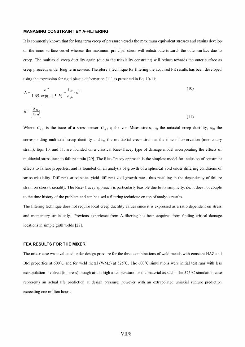
MANAGING CONSTRAINT BY -FILTERING
It is commonly known that for long term creep of pressure vessels the maximum equivalent stresses and strains develop
on the inner surface vessel whereas the maximum principal stress will redistribute towards the outer surface due to
creep. The multiaxial creep ductility again (due to the triaxiality constraint) will reduce towards the outer surface as
creep proceeds under long term service. Therefore a technique for filtering the acquired FE results has been developed
using the expression for rigid plastic deformation [11] as presented in Eq. 10-11;
cr
fm
fucr
h)5.1exp(65.1
qh kk
3
(10)
(11)
Where kk is the trace of a stress tensor ij , q the von Mises stress, fu the uniaxial creep ductility, fm the
corresponding multiaxial creep ductility and m the multiaxial creep strain at the time of observation (momentary
strain). Eqs. 10. and 11. are founded on a classical Rice-Tracey type of damage model incorporating the effects of
multiaxial stress state to failure strain [29]. The Rice-Tracey approach is the simplest model for inclusion of constraint
effects to failure properties, and is founded on an analysis of growth of a spherical void under differing conditions of
stress triaxiality. Different stress states yield different void growth rates, thus resulting in the dependency of failure
strain on stress triaxiality. The Rice-Tracey approach is particularly feasible due to its simplicity. i.e. it does not couple
to the time history of the problem and can be used a filtering technique on top of analysis results.
The filtering technique does not require local creep ductility values since it is expressed as a ratio dependent on stress
and momentary strain only. Previous experience from -filtering has been acquired from finding critical damage
locations in simple girth welds [28].
FEA RESULTS FOR THE MIXER
The mixer case was evaluated under design pressure for the three combinations of weld metals with constant HAZ and
BM properties at 600°C and for weld metal (WM2) at 525°C. The 600°C simulations were initial test runs with less
extrapolation involved (in stress) though at too high a temperature for the material as such. The 525°C simulation case
represents an actual life prediction at design pressure, however with an extrapolated uniaxial rupture prediction
exceeding one million hours.
VII/8

The results were studied at 1000 hours for the 600°C simulations and at 100 000 h for the 525°C simulation. The
runtime of the steam mixer simulation to 100 000h was 8 hours of CPU time (8 h 20 minutes of wall clock time) with
an 3.80GHz Intel Xeon PC.
The selected time of study for the 600°C cases was determined through a simple Larson-Miller time-temperature
transformation. At the selected simulation time strains, stresses and “creep exhaustion” ( -values as defined by Eq. 10.)
were determined (see Table 2).
Table 2. Creep exhaustion localisation (critical location), maximum calculated -value, von Mises stress and maximum
principal strain at the specified location.
Case Critical location maximum -value VM (MPa)1
(%)
600°C
WM1
saddle point surface
(HAZ)0.015 54 0.5
600°C
WM2
saddle point surface
(HAZ)0.018 56 0.7
600°C
WM3
overflow at 422 h
shear in WM- - >20
525°C
WM2
saddle point surface
(HAZ)0.015 57 0.6
The 525°C simulation results ( -values, maximum principal strain and von Mises stress) are presented in Fig. 5-Fig. 7.
VII/9

Fig. 5. Creep exhaustion ( -values) after 100 000 h / 525°C.
Fig. 6. Creep strain (maximum principal) after 100 000 h / 525°C, note location (inner surface BM)
VII/10

Fig. 7. Stress (von Mises) after 100 000 h / 525°C, note location (inner surface WM)
The maximum -values acquired from the simulations with WM1 and WM2 seem low but when divided with values
for uniaxial creep fracture strain as in Eq. 10, the consumed creep strain can be attained (see Table 3). At the point of
observation (100 000 h) the results are very reasonable for expected low ductility in uniaxial long term tests of cross
welds.
Table 3. Consumed creep strain (% of available) in the critical HAZ location of Fig. 5 after 100 000 h of service
(design pressure) as a function of uniaxial creep ductility.
Uniaxial creep ductility Consumed creep strain
10 % 15 %
8 % 19 %
6 % 25 %
4 % 37 %
2 % 75 %
1.5 % 100 %
As earlier stated the filtering technique as such does not require local creep ductility values since it is expressed as ratio
dependent on stress and momentary multiaxial creep strain. The 600°C simulations with different WM show the
difference in damaging mechanism. The weld with a over-matched weld metal (WM2) shows maximum -values in the
outer HAZ saddle point surface (see Fig. 8) and the weld with a very weak weld metal (WM3) fails prematurely due
to extensive deformation in the WM (see Fig. 9).
VII/11

Fig. 8. Creep exhaustion after 1000 h at 600°C with over-matched weld metal (WM2). Compare with 525°C
simulation in Fig. 5.
Fig. 9. Creep exhaustion after 422 h at 600°C with weak weld metal (WM3). Note the failing weld metal.
VII/12

DISCUSSION AND CONCLUSIONS
The LCSP creep strain model has been used for the steam mixer simulations, including primary to tertiary creep. The
ABAQUS implementation of the model is working smoothly with satisfactory processing time. The numerical analysis,
especially utilising the -filtering technique seems to accurately pinpoint the critical damage locations of the steam
mixer. The 3-zone weld simulation (BM, WM and HAZ) produce differing amounts of damage and a change of critical
location depending on selected WM properties. Earlier inspection data exists for the case mixer and also for another
mixer in the same power plant. This data will eventually be used for further calibration of the filtering technique. The
current of the -filter seem to work well for estimating the consumed creep strain but other forms more suitable for
creep such as the creep ductility functions proposed by Cocks and Ashby referenced in [18], Andreas [13] or Spindler
[14] should be tested for improved results. In conclusion it is quite evident that a powerful tool for high temperature
component life assessments has been created and that advanced multiaxial creep modelling can now be performed with
only a minimum amount of actual strain data. This feature will be especially handy for modelling structures with new
materials with limited data and for pinpointing critical locations in components in service, thus improving inspection
targeting. The new FEA tools will in the near future also be used for assessing large components made of P91 and X20
steels.
ACKNOWLEDGEMENT
The support of the Academy of Finland, decision nr. 117700 (Prof. Kim Wallin) is gratefully acknowledged. Fortum
Power & Heat is also gratefully acknowledged for all support related to the steam mixer case study.
REFERENCES
[1] Holmström S, Laukkanen A, Calonius K, Weldment matching for creep life of P22 and P91 girth welds. Conf.
on Integrity of high temperature welds, 24-26 April 2007, London UK
[2] Hayhurst D. The use of computational creep continuum damage mechanics to optimise materials selection for
high temperature weldments, Modelling Simul. Mater. Eng. 2, 1994, p.421-438.
[3] Perrin I, Hayhurst D, A method for the transformation of creep constitutive equations, Int. J. Pres. Ves. &
Piping 68, 1996, p299-309.
[4] Perrin I, Hayhurst D, Ainsworth A, Approximate creep rupture lifetimes for butt welded steel pressurised
pipes. Eur. J. Mech. a/Solids 19, 2000, p.223-258.
VII/13

[5] Law M, Payten W, Weld performance under creep using finite element modelling, Int. J. Pres. Ves. & Piping
72, 1997, p45-49
[6] Law M, Payten W, Snowden S, Creep Modeling of welded joints using the theta projection concept and finite
element analysis, Journal of Pressure Vessel Technology, ASME transactions Vol. 122, 2000, p. 22-26.
[7] Hyde T.H, Sun W, Life prediction of repair welds in pressurised CrMoV pipe with incorporation of initial
damage, Int. J. Pres. Ves. & Piping 81, 2004, p1-12
[8] Wu R, Sandström R, Seitisleam F, Influence of extra coarse grains on the creep properties of 9 percent CrMoV
(P91) steel weldment, Journal of engineering and technology, Transactions of ASME Vol. 126, p. 87-94.
[9] Becker A, Hyde T, Sun W, Andersson P, Benchmark for finite element analysis of creep continuum damage
mechanics, Comp. Mat. Sci. 25, 2002, p 34-41.
[10]Law M, Payten W, Small R, Modelling the creep behaviour of reheat header longitudinal weld, Int. J. Pres.
Ves. & Piping 77, 2000, p.99-103.
[11]Hurst R.C, Rantala J.H. Influence of multiaxial stresses on creep and creep rupture of tubular components,
ASM Handbook, Vol. 8, 2000 p. 405-411
[12]Webster G., Holdsworth S., Loveday M., Nikbin K., Perrin I., Purper H., Skelton R., Spindler M., Fatigue &
Fracture of Engineering Materials & Structures, Volume 27, Number 4, April 2004 , pp. 319-342(24),
Publisher: Blackwell Publishing
[13]Andreas, W. Evaluation of creep damage due to woid growth under traxial stress states in the design of steam
turbine components. JSME. IntJ. Ser A 45, p. 72-77.
[14]Spindler M.W. The multiaxial creep ductility of austenitic stainless steels. Fatigue Fract Engng Mater Struct
27, 2004. p. 273-281.
[15]R5 (2001) Assessment procedure for the high temperature response of structures. British Energy, Glouchester
UK.
[16]ASME (2000) Section III Div. 1. Sub-Section NH, ASME, New York, USA
[17]RCC-MR (1987) Design and construction rules for mechanical components of FBR nuclear islands, Paris
France.
[18]Holmström S, Auerkari P, Robust prediction of full creep curves from minimal data and time to rupture,
submitted to Energy Materials; Materials Science and Engineering for Energy Systems.
doi:10.1179/174892406X173594, 2006, Vol 1. p249-255
VII/14
[19]Holmström, S., Auerkari, P., Holdsworth S. Predicting creep strain response from rupture data and robust
creep curve model. International Conference on Life Management and Maintenance for Power Plants.
Helsinki-Stockholm-Helsinki, 12-14 June 2007. Vol 1.
[20]Holmström, S., Laukkanen A., Calonius, K., Visualising creep exhaustion in a P22 girth weld. International
Conference on Life Management and Maintenance for Power Plants. Helsinki-Stockholm-Helsinki, 12-14 June
2007. Vol 2. pp.208-221
[21]Webster G.A. High Temperature Component life assessment. Department of Mechanical Engineering, Imperial
Collage of Science, ISBN 0-412-58520-0, Chapman & Hall. 1994, p.37-38
[22]EN 10162, 2002. Seamless steel tubes for pressure purposes. Technical delivery conditions. Part 2: Non-alloy
and alloy steel tubes with specified elevated temperature properties. CEN, Brussels.
[23]Holdsworth, S.R., 1996b. ECCC-WG1 Recommendations, Volume 5, Guidance for the Assessment of Creep
Rupture, Creep Strain and Stress Relaxation Data, ECCC Document 5524:MC:38 Issue 3.
[24]Holdsworth S., Davies R., A recent advance in the assessment of creep rupture data Nuclear Engineering and
Design, Volume 190, Issue 3, 2 June 1999, Pages 287-296
[25]DIN 17243. 1987. Weldable heat resisting steel forgings and rolled or forged steel bars; Technical delivery
conditions. Deutche Institut für Normung E.V.
[26]Rantala, Juhani; Salonen, Jorma; Auerkari, Pertti; Holmström, Stefan; Lehtinen, O.; Pitkänen, M.; Nikkarila,
R. Life extension of hot steam piping after 200 000 h of service. Energy Materials: Materials Science &
Engineering for Energy Systems. Vol. 2 (2007) No: 2, 104-108(5)
[27]ABAQUS. 2007. ABAQUS Online Documentation: Version 6.7-1, Theory Manual [CD-ROM]. ABAQUS
Inc.
[28]Holmström S., Laukkanen A., Calonius K., Finding critical damage locations by -filtering in finite-
elementmodelling of a girth weld, In press: Mater. Sci. Eng. A (2009), doi:10.1016/j.msea.2008.04.107
[29]Rice, J.R. and Tracey, D.M., On the Ductile Enlargement of Voids in Triaxial Stress Fields, Journal of the
Mechanics and Physics of Solids, Vol. 17, Issue 3, 1969, Pages 201-217.
VII/15


Series title, number and report code of publication
VTT Publications 728 VTT-PUBS-728
Author(s) Stefan Holmström Title
Engineering Tools for Robust Creep Modeling
Abstract High temperature creep is often dealt with simplified models to assess and predict the future behav-ior of materials and components. Also, for most applications the creep properties of interest require costly long-term testing that limits the available data to support design and life assessment. Such test data sets are even smaller for welded joints that are often the weakest links of structures. It is of considerable interest to be able to reliably predict and extrapolate long term creep behavior from relatively small sets of supporting creep data.
For creep strain, the current tools for model verification and quality assurance are very limited. The ECCC PATs can be adapted to some degree but the uncertainty and applicability of many models are still questionable outside the range of data. In this thesis tools for improving the model robustness have been developed. The toolkit includes creep rupture, weld strength and creep strain modeling improvements for uniaxial prediction. The applicability is shown on data set consisting of a selection of common high temperature steels and the oxygen-free phosphorous doped (OFP) copper. The steels assessed are 10CrMo9-10 (P22), 7CrWVMoNb9-6 (P23), 7CrMoVTiB10-10 (P24), 14MoV6-3 (0.5CMV), X20CrMoV11-1 (X20), X10CrMoVNb9-1 (P91) and X11CrMoWVNb9-1-1 (E911).
The work described in this thesis has provided simple yet well performing tools to predict creep strain and life for material evaluation, component design and life assessment purposes. The uncer-tainty related to selecting the type of material model or determining weld strength factors has been reduced by the selection procedures and by linking the weld behavior to the base material master equation. Much of the resulting improvements and benefits are related to the reduced requirements for supporting creep data. The simplicity and robustness of the new tools also makes them easy to implement for both analytical and numerical solutions. ISBN 978-951-38-7378-3 (soft back ed.) 978-951-38-7379-0 (URL: http://www.vtt.fi/publications/index.jsp)
Series title and ISSN Project number
VTT Publications 1235-0621 (soft back ed.) 1455-0849 (URL: http://www.vtt.fi/publications/index.jsp)
36468
Date Language Pages January 2010 English 94 p. + app. 53 p.
Name of project Commissioned by SA-KWAK jatko
Keywords Publisher Creep, strain, damage, modeling, steel, OFP copper
VTT Technical Research Centre of Finland P. O. Box 1000, FI-02044 VTT, Finland Phone internat. +358 20 722 4520 Fax +358 20 722 4374


Julkaisun sarja, numero ja raporttikoodi
VTT Publications 728 VTT-PUBS-728
Tekijä(t) Stefan Holmström
Nimeke
Virumismallinnuksen uudet menetelmät
Tiivistelmä Rakenteiden suunnitteluun ja elinikäennusteisiin käytetyt kuumalujien terästen lujuusarvot ja hitsien lujuuskertoimet pohjautuvat virumiskoetuloksiin, joita on varsinkin pitkäaikaisina käytettävissä usein vain niukasti. Sen vuoksi on erityisen tärkeää, että koetuloksiin sovitetut materiaalimallit ovat talou-dellisia, tarkkoja ja luotettavia erityisesti ekstrapoloitaessa pidemmille käyttöajoille.
Tässä väitöstyössä on kehitetty uusia malleja työkaluiksi virumismurtolujuuden, hitsien lujuusker-toimien ja virumisvenymän luotettavaan määrittämiseen sekä virumiseliniän ennustamiseen erityi-sesti tapauksissa, joissa mallinnuksen tueksi on käytettävissä niukasti virumiskoetuloksia. Uusien mallien suorituskykyä on testattu eurooppalaisessa vertailututkimuksessa, jossa ne ennustivat yk-sin-kertaisesta muodostaan huolimatta venymiä tarkemmin kuin aiemmat ja huomattavasti moni-mutkaisemmat virumismallit. Uusia malleja on työssä sovellettu OFP-kuparille ja ferriittisille teräksil-le 10CrMo9-10 (P22), 7CrWVMoNb9-6 (P23), 7CrMoVTiB10-10 (P24), 14MoV6-3 (0.5CMV), X20CrMoV11-1 (X20), X10CrMoVNb9-1 (P91) ja X11CrMoWVNb9-1-1 (E911). Materiaalimalleja on myös sovitettu numeerisen suunnittelun työkaluihin (COMSOL ja ABAQUS) ja verifioitu pitkään käytössä olleen hitsatun putkiyhteen elinikätarkastelulla.
Väitöstyön tuloksena kehitettyjä malleja ja menetelmiä voivat soveltaa korkean lämpötilan raken-teiden suunnittelijat ja eliniän hallinnan asiantuntijat helpottamaan ja tarkentamaan virumiskäyttäy-tymisen ennustamista. Työn keskeinen anti on kehitettyjen menetelmien tarjoama vähentynyt mate-riaalidatan tarve ja mallien yksinkertainen rakenne, joka helpottaa niiden hyödyntämistä sekä ana-lyyttisissä että numeerisissa ratkaisuissa.
ISBN 978-951-38-7378-3(nid.) 978-951-38-7379-0 (URL: http://www.vtt.fi/publications/index.jsp)
Avainnimeke ja ISSN Projektinumero VTT Publications 1235-0621 (nid.) 1455-0849 (URL: http://www.vtt.fi/publications/index.jsp)
36468
Julkaisuaika Kieli Sivuja Tammikuu 2010 Englanti, suom. tiiv. 94 s. + liitt. 53 s.
Projektin nimi Toimeksiantaja(t) SA-KWAK jatko
Avainsanat Julkaisija
Creep, strain, damage, modeling, steel, OFP copper
VTT PL 1000, 02044 VTT Puh. 020 722 4520 Faksi 020 722 4374


Dissertation VTT PUBLICATIONS 728VTT CREATES BUSINESS FROM TECHNOLOGYTechnologyandmarketforesight•Strategicresearch•Productandservicedevelopment•IPRandlicensing•Assessments,testing,inspection,certification•Technologyandinnovationmanagement•Technologypartnership
•••VTTPUB
LICA
TION
S728ENG
INEER
ING
TOO
LSFOR
RO
BU
STCR
EEPMO
DELIN
G
ISBN 978-951-38-7378-3 (soft back ed.) ISBN 978-951-38-7379-0 (URL: http://www.vtt.fi/publications/index.jsp)ISSN 1235-0621 (soft back ed.) ISSN 1455-0849 (URL: http://www.vtt.fi/publications/index.jsp)
Stefan Holmström
Engineering Tools for Robust Creep Modeling
Creep models are needed for design and life management of structural components operating at high temperatures. The determination of creep properties require long-term testing often limiting the amount of data. It is of considerable interest to be able to reliably predict and extrapolate long term creep behavior from relatively small sets of creep data. In this thesis tools have been developed to improve the reliability of creep rupture, creep strain and weld strength predictions. Much of the resulting improvements and benefits are related to the reduced requirements for supporting creep data. The simplicity and robustness of the new tools also make them easy to implement in analytical and numerical solutions. Creep models for selected high temperature steels and OFP copper are presented.