Direct Use Geothermal Applications For Brazed Plated Heat ...

CHAPTER 17ENGINEERING COST
ANALYSISCharles V. HigbeeGeo-Heat Center
Klamath Falls, OR 97601
17.1 INTRODUCTION
In the early 1970s, life cycle costing (LCC) wasadopted by the federal government. LCC is a method ofevaluating all the costs associated with acquisition, con-struction and operation of a project. LCC was designed tominimize costs of major projects, not only in considerationof acquisition and construction, but especially to emphasizethe reduction of operation and maintenance costs during theproject life.
Authors of engineering economics texts have been veryreluctant and painfully slow to explain and deal with LCC.Many authors devote less than one page to the subject. Thereason for this is that LCC has several major drawbacks.The first of these is that costs over the life of the projectmust be estimated based on some forecast, and forecastshave proven to be highly variable and frequently inaccurate.The second problem with LCC is that some life span mustbe selected over which to evaluate the project, and manyprojects, especially renewable energy projects, are expectedto have an unlimited life (they are expected to live forever).The longer the life cycle, the more inaccurate annualcosts become because of the inability to forecast accurately.
This chapter on engineering cost analysis is designedto provide a basic understanding and the elementary skillsto complete a preliminary LCC analysis of a proposedproject. The time value of money is discussed and mathe-matical formulas for dealing with the cash flows of a projectare derived. Methods of cost comparison are presented.Depreciation methods and depletion allowances are inclu-ded combined with their effect on the after-tax cash flows.The computer program RELCOST, designed to performLCC for renewable energy projects, is also presented. Adiscussion of caveats related to performing LCC is included.No one should attempt to do a comprehensive cost analysisof any project without an extensive background on thesubject, and considerable expertise in the current tax law.
17.1.1 Use of Interest Tables
When performing engineering cost analysis, it isnecessary to apply the mathematical formulas developed inthis chapter and avoid using interest tables for the followingreasons:
1. Interest rates applying to real world problems are notfound in interest tables, and therefore, interpolationis required.
When trying to solve problems with interpolation theassumption is made that compound interest formulasare linear functions. THEY ARE NOT. They arelogarithmic functions.
2. Not only are real world interest rates difficult to find intables, but it is frequently difficult to find the requirednumber of interest periods for the project in a set oftables.
3. If the need arises to convert a frequently compoundedinterest rate to a weekly or monthly interest rate, it isalmost certain the value of the effective interest ratewill not be in any interest table.
4. Renewable energy projects, especially those for districtheating systems, can run into hundreds of millions ofdollars. Although it is understood that this chapter waswritten for preliminary economic studies, nevertheless,interpolation of interest tables can cause an error manytimes larger than the cost analyst's annual salary.
5. With today's microcomputers and sophisticated hand-held calculators, interest tables are obsolete. Calcula-tors capable of computing all time value functionsexcept gradients are available for under $20. Thesecalculators can also solve the number of interest per-iods and iterate an interest rate to nine decimal places.
17.2 THE TIME VALUE OF MONEY
The concept of the time value of money is as old asmoney itself. Money is an asset, the same as plant andequipment and other owned resources. If equipment isborrowed, a plant is rented or land is leased, the ownershould receive equitable compensation for its use. If moneyis borrowed, the lender should be reimbursed for its use.The rent paid for using someone else's money is calledinterest. Interest takes two different forms: simple interestand compound interest.
359
Throughout this chapter, the time value of money andcompound interest are used in the cost analysis of projects.Such things as risk and uncertainty are ignored, and theconcept of an unstable dollar or the value of the dollarfluctuating in the foreign market are not considered.However, in LCC analysis of renewable energy projects,inflation rates for operation and maintenance, equipmentpurchases, energy consumed and the revenue from energysold for both conventional and renewable energy, will beconsidered.
The concept of the time value of money evolves fromthe fact that a dollar today is worth considerably more thana promise to pay a dollar at some future date. The reasonthis is true is because a dollar today could be invested and beearning interest such that, at sometime in the future, theinterest earned would make the investment worthconsiderably more than one dollar. To illustrate the timevalue of money, it is convenient to consider money investedat a simple interest rate.
17.2.1 Simple Interest
Simple interest is interest accumulated periodically ona principal sum of money that is provided as a loan orinvested at some rate of interest (i), where i represents aninterest rate per interest period. It is important to notice thatin problems involving simple interest, interest is onlycharged or earned on the original amount borrowed orinvested. Consider a deposit of $100 made into an accountthat pays 6% simple interest annually. If the money is lefton deposit for 1 year, the balance at the end of year onewould be:
100 + 0.06(100) = $106.
If the money is left on deposit for 2 years, the balanceat the end of year two would be:
100 + 0.06(100) + 0.06(100) = $112.
If the money is left on deposit for 3 years, the balanceat the end of year three would be:
100 + 0.06(100) + 0.06(100) + 0.06(100) = $118.
If n equals the number of interest periods the money isleft on deposit and i equals the rate of interest for eachperiod, the formula for calculating the balance at the end ofn periods would be:
100 + 100(i x n).
Substituting 6% for i and 3 for n, the formula becomes:
100 + 100(0.06 x 3) = $118.
360
Substituting present value (Pv) for the amount ofmoney loaned or deposited at time zero (beginning of thetime period covered by the investment), and future value(Fv) for the balance in the account at the end of n periods,the formula becomes:
Fv = Pv + Pv(i x n).
Factoring out Pv, the formula becomes:
Fv = Pv(1 + i x n). (17.1)
Going back to the original values, if the $100 is left ondeposit for 5 years, the future value would be $130, and iswritten:
Pv = 100; i = 0.06; n = 5Fv = 100(1 + 0.06 x 5)Fv = $130.
Remember, in simple interest problems, interest isearned only on the amount of the original deposit. Considerthe case where interest is calculated more frequently thanonce per year. This would not change the amount of moneyearned in simple interest calculations.
Suppose that $100 was deposited for 5 years at a rate of6% simple interest, calculated every three months. Sincethere are four 3-month periods in a year, the simple interestper interest period becomes 0.06/4 = 0.015 and n becomes4 quarters per year x 5 y = 20 total interest periods.Therefore:
Fv = 100(1 + 0.015 x 20)Fv = $130.
Applying this formula to the time value of money, itcan be shown that for any given rate of interest, $100received today would be much greater value than $100received 5 years from today. Consider:
Proposal 1: A promise to pay $100 5 years from today.Proposal 2: A promise to pay $100 today.
If proposal 2 is accepted over proposal 1, the $100received today could be deposited into an account thatearned 9% annually, and in 5 years the balance would be$145. Using this same theory, the present value of apromise to pay $100 5 years from today can be evaluated as:
Fv = 100; i = 0.09; n = 5 y100 = Pv(1 + 0.09 x 5).
Solving for Pv, the equation becomes:
Pv = 100/(1 + 0.09 x 5)Pv = $68.97.

Throughout this chapter and in cost analysis texts ingeneral, cash flow diagrams are normally drawn to illustratemonies flowing into or out of a project at some specific timeperiod. The accepted convention is: a) money flowing outis indicated by a down arrow and b) money flowing in isindicated by an up arrow.
Example 17.1: A $1,000 loan to be repaid in twoequal annual payments, from the borrower's point of view,would be drawn as:
and, from the lender's point of view, would be drawn as:
The examples below illustrate the application of cashflow diagrams.
Example 17.2: A woman deposited $500 for 3 yearsat 7% simple interest per annum. How much money can bewithdrawn from the account at the end of the 3-year period?The cash flow diagram below indicates money depositedinto the investment as i, and money withdrawn from theinvestment as h,
solution:
Fv = Pv(1 + i x n)Fv = 500(1 + 0.07 x 3)Fv = 500(1.21)Fv = $605.
Example 17.3: Assume $500 is deposited for 200 daysin an account that earns 6% simple interest per annum.What is the balance at the end of the investment period?The solution is:
Fv = Pv(1 + i x n)Fv = 500[1 + 0.06(200/365)]Fv = 500(1.0329)Fv = $516.45.
17.2.2 Compound Interest
All compound interest formulas developed will includethe standard functional notation for those formulas to theright of the developed formula. Functional notation is a
shorthand method of representing a formula to be applied toa problem or a portion of a problem, rather than having towrite the formula in its entirety.
For example, (F/P, i, n) is read, "To find the futurevalue F, given the present value, P at an interest rate perperiod i for n interest periods." This notation applies onlyto compound interest.
Compound interest varies from simple interest in thatinterest is earned on the interest accumulated in the account.To illustrate:
If $100 is deposited at 6% compound annually, at theend of the first year the balance would be:
100(1 + 0.06) = $106.
This is the same as in simple interest. However, if themoney is allowed to remain on deposit for 2 years, theinterest earned during the second year would be:
106(0.06) = $6.36
giving a balance of $112.36 at the end of the second year.If the money is left on deposit for 3 years, the interest earnedduring the third year would be:
112.36(0.06) = $6.74.
Thus, the balance at the end of the third year would be:
100 + 6 + 6.36 + 6.74 = $119.10.
The mathematical function of compound interest for adeposit of $100 earning 6% compounded annually left ondeposit for 3 years is stated and described mathematicallybelow.
Original deposit plus interest earned at the end of thefirst year becomes:
Fv = 100(1 + 0.06)
plus the interest earned during the second year:
+ 0.06[100(1 + 0.06)]
plus the interest earned during the third year:
+0.06{100(1 + 0.06) + 0.06[100(1 + 0.06)]}.
The formula becomes rather complex with only a 3-year investment. The formula can be simplified throughmathematical manipulation. For purposes of this illustra-tion, let 0.06 = i and the number of interest periods = 3,then:
Fv = 100(1 + i) + i[100(1 + i)] + i{100(1 + i) + i [100(1 + i)]}.
361
Factoring out $100 from the above equation:
Fv = 100[(1 + i) + i(1 +i) + i{(1 + i) + i(1 + i)}]
simplifying:
Fv = 100[1 + i + i + i2 + i(1 + i + i + i2)]
simplifying further:
Fv = 100(1 + i + i + i2 + i + i2 + i2 + i3)
and collecting terms:
Fv = 100(1 + 3i + 3i2 + i3)
then, this equation can be factored into:
Fv = 100[(1 + i)(1 + i)(1 + i)] = 100(1 + i)3.
Substituting n for the number of interest periods, whichin this case is 3, the result is:
Fv = 100(1 + i)n.
Letting Pv = the amount of the investment, then:
Fv = Pv(1 + i)n (F/P,i,n)(17.2)
This is the single payment compound amount factor.
Solving Equation (17.2) for Pv gives:
(P/F,i,n)(17.3)
which is the single payment present worth factor.
With the development of the equation for finding thefuture value of a lump sum investment at a compoundinterest rate for n interest periods, it can be shown how morefrequent compounding increases the interest earned.
An interest rate of 3%/6 mo would be stated in nominalform as 6% compounded semiannually.
Consider the following examples with interest ratesstated as an annual percentage rate (APR), commonlyreferred to as the "nominal interest rate."
Example 17.4: An amount of $100 is invested for 3years in an account that earns 18% compounded annually.The future value at the end of the 3-year period will be:
Fv = Pv(1 + i)n
Fv = 100(1 + 0.18)3
Fv = 100(1.6430)Fv = $164.30.
362
Example 17.5: Assume $100 is invested for threeyears in an account that earns 18% compounded quarterly.The future value at the end of the 3-year period is:
Fv = Pv(1 + i)n
where
i = 0.18/4 quarters/y = 0.045 per quartern = 3 y x 4 quarters/y = 12 interest periods.
Solution:
Fv = 100(1 + 0.045)12
Fv = 100(1.6959)Fv = $169.59.
Example 17.6: Suppose $100 is invested in an accountthat earns 18% compounded monthly. The future value atthe end of a 3-year period is:
Fv = Pv(1 + i)n
where
i = 0.18/12 months/y = 0.015/mon = 3 y x 12 mo/y = 36 interest periods.
Solution:
Fv = 100(1 + 0.015)36
Fv = 100(1.7091)Fv = $170.91.
Example 17.7: An amount of $100 is invested for 3years in an account that earns 18% compounded weekly.The future value at the end of the 3-year period is:
Fv = Pv(1 + i)n
where
i = 0.18/52 weeks/y = 0.0034615/weekn = 3 y x 52 weeks/y = 156 weeks.
Solution:
Fv = 100(1 + 0.0034615)156
Fv = 100(1.7144)Fv = $171.44.
Example 17.8: If $100 is invested for 3 years in anaccount that earns 18% compounded daily, the future valueat the end of the 3-year period is:
Fv = Pv(1 + i)n

where
i = 0.18/365 days/y = 0.00049315/dn = 3 y x 365 d/y = 1095 d.
Solution:
Fv = 100(1 + 0.00049315)1095
Fv = 100(1.71577)Fv = $171.58.
Money invested today will grow to a larger amount inthe future. If this is true, then the promise to pay someamount of money in the future is worth a smaller amounttoday.
Example 17.9: What is the present value of a promiseto pay $3,000 5 years from today if the interest rate is 12%compounded monthly? This can be written:
where
i = 0.12/12 = 0.01n = 5 x 12 = 60.
Solution:
Pv = 3,000/(1 + 0.01)60
Pv = $1,651.35.
17.2.3 Annual Effective Interest Rates
It is convenient at this point in the development ofcompound interest to introduce annual effective interestrates. Annual effective interest (AEI) is interest stated interms of an annual rate compounded yearly, which is theequivalent of a nominally stated interest rate. Table 17.1illustrates the relationship between nominal interest, interestrate per interest period, and annual effective interest.
Notice that the nominal interest rate remains the samepercentage while the compounding periods change. Theinterest rate per interest period is obtained by dividing thenominal rate by the number of interest periods per year. Theannual effective interest rate is the only true indicator of theamount of annual interest, and therefore, annual effectiveinterest provides a true measure for comparing interest rateswhen the frequency of compounding is different.
The annual effective interest rate may be found for anynominal interest rate as shown below.
Table 17.1 Comparative Interest Rates______________________________________________
(APR) Nominal Interest Rate per Annual Effective Interest Rate Interest Period Interest (AEI) (18%) (%) (%) Compound 18.00 18.00 annually
Compounded 9.00 18.81 semiannually
Compounded 4.50 19.25 quarterly
Compounded 1.50 19.56 monthly
Compounded 0.346 19.71 weekly
Compounded 0.04932 19.716 daily
Compounded 19.7217 continuously______________________________________________
Consider a dollar that was invested for 1 year at anominal rate of 18% compounded monthly. To calculate thebalance (Fv) at the end of the year:
Fv = 1[1 + (0.18/12)]12
therefore,
Fv = 1(1.015)12
Fv = 1(1.1956)Fv = $1.1956.
Because a dollar was invested originally, the annualinterest earned may be found by subtracting the originalinvestment:
1.1956 - 1 = 0.1956
and the effective interest is 19.56%. Then, the formula forfinding annual effective interest is:
(17.4)
363

where
AEI = annual effective interest rater = nominal interest rate/ym = number of interest periods/y.
The annual percentage rate is divided by the number ofcompounding periods/y and raised to the power of thenumber of compounding periods/y, and 1 is subtracted fromthat answer to arrive at the annual effective interest rate.
The following examples are used to further illustratethe differences between APR and AEI.
Example 17.10: For an APR of 12% compoundedannually, the annual effective interest (AEI) is 12%.Therefore:
AEI = 12% compounded annually. There is no difference between the two.
Example 17.11: For an APR of 12% compoundedsemi-annually, the semiannual effective interest rate is0.12/2 = 0.06 or 6%, presented as:
AEI = (1 + 0.12/2)2 - 1 = 0.1236 or 12.36%.
Example 17.12: For an APR of 12% compoundedquarterly, the quarterly effective interest rate is 0.03 or 3%,AEI becomes:
AEI = (1 + 0.12/4)4 - 1 = 0.1255 or 12.55%.
Example 17.13: For an APR of 12% compoundeddaily, the daily effective interest rate is 0.12/365 = 0.003288or 0.3288%, giving:
AEI = (1 + 0.12/365)365 - 1 = 0.12747 or 12.75%.
When interest is compounded continuously (when napproaches infinity), the annual effective interest rate takesthe form of e - 1, where e = the natural logarithm2.7182818. Therefore, an APR of 12% compoundedcontinuously would yield an AEI of (2.7182818)0.12 - 1 =12.749%.
Effective interest rates can be calculated for periodsother than annually.
To find a weekly effective interest rate of 12%compounded daily, the weekly effective interest rate wouldbe:
(1 + 0.12/365)7 - 1 = 0.0023, or 0.23%.
Therefore,
(17.5)
364
where
r = annual percentage ratem = number of compound periods/yearc = number of compound periods for the time frame of the effective interest rate.
Example 17.14: The present value of a promise to pay$4,000 6 years from today at an interest rate that iscompounded quarterly is $2,798. Find the nominal interestrate and the annual effective interest rate.
Fv = Pv(1 + i)n
where
n = 6 x 4 = 24 quarters
and solving
4,000 = 2,798(1 + i)24
dividing both sides by 2,798
1.42959 = (1 + i)24
taking the 24th root of both sides
(1.42959)0.04167 = [(1 + i)24]0.04167
1.015 = 1 + i
i = 0.015, or 1.5%.
By definition, i is the interest rate per interest period.Therefore, the answer, 1.5%, is the interest rate per quarter.In order to find the nominal interest rate (or annualpercentage rate), it is necessary to multiply i times thenumber of quarters per year. The nominal interest rate is0.015 x 4 = 0.06, or 6% compounded quarterly. The answerwould be incorrect if the frequency of compounding was notincluded. If the nominal rate is given as 6%, this wouldindicate 6% compounded annually.
The annual effective interest rate, using Equation(17.4), becomes:
AEI = (1 + 0.015)4 - 1
AEI = 0.0614, or 6.14%.

Years
5
10
15 20 25 3530 4010
20
30
40
50
60
70
80
90
100
4%
6%
8%
10%
12%
Figure 17.1 Exponential nature of compound interest rates.
The formulas developed for compound interest and thesimilar formula for converting APR to AEI are logarithmicfunctions (see Figure 17.1).
When interest rates are extremely low, the number ofcompounding periods is almost insignificant. For example,2% APR compounded annually is 2% AEI; 2% APRcompounded daily is 2.02% AEI while 40% APRcompounded daily jumps to 49.15% AEI.
In evaluating projects for nonprofit organizations,interest rates are usually kept rather low, but there are manyprivate entities that evaluate alternatives at the corporation’srate of return, which can be a very high rate.
17.3 ANNUITIES
17.3.1 Ordinary Annuities
The definition of an ordinary annuity is a stream ofequal end-of-period payments. Ordinary annuities are themost common form of payment series used in cost analysis.Loan payments, car payments, charge card payments,maintenance and operating costs of equipment are all statedin terms of ordinary annuities. These payments arefrequently monthly payments, but they can be weekly, yearlyor any other uniform time period. The important thing isthat they begin at the end of the first interest period. Forexample, a person purchases an automobile for $5,000 andis obligated to pay $125 per month for 48 months. The firstpayment will be due one month after the purchase of the carand the last payment will be due at the end of month 48. Inorder to derive a mathematical formula to evaluate ordinaryannuities, it is convenient to use the future value formula forcompound interest Equation (17.2).
Consider three equal end-of-year payments of $100each.
To find the future value of this payment series at theend of year three, use the future value formula. Notice thatthe first payment is two interest periods before the end of theproject. Therefore, the future value of the first payment is:
Fv = Pv(1 + i)n
Fv = 100(1 + i)2.
The future value of the second payment, which is oneinterest period before the end of the project, is:
Fv = 100(1 + i)1.
The third payment is zero interest periods away fromthe end of the project. Therefore, the future value ofpayment number three is simply $100. The future value ofall three payments is:
Fv = 100(1 + i)2 + 100(1 + i)1 + 100.
Reversing the order of these terms and factoring out$100, the equation becomes:
Fv = 100[1 + (1 + i)1 + (1 + i)2].
365

Notice that with a 3-year project and three annualpayments, n does not get higher than 2. This is because thepayments are made at the end of each period. Letting A =the amount of each payment, a general equation can bewritten to find the future value of n payments as:
Fv = A[1 + (1 + i)1 + (1 + i)2 + (1 + i)3 +...+ (1 + i)n-1].
Multiplying this equation by (1 + i) results in:
Fv(1 + i) = A[(1 + i)1 + (1 + i)2 + (1 + I)3
+ (1 + i)4 +...+ (1 + i)n].
Subtracting the first equation from the second equation:
Fv(1 + i) - Fv = A[-1 + (1 + i)n]
also
Fv + i(Fv) - Fv = A[(1 + i)n - 1]
and
i(Fv) = A[(1 + i)n - 1]
dividing both sides of the equation by i gives:
(F/A,i,n)(17.6)
This is the uniform series compound amount factor.
Solving for A instead of Fv gives:
(A/F,i,n)(17.7)
This the uniform series sinking fund factor.
Returning to the future value formula, Fv = Pv(1 + i)n,and substituting the right side of this equation for Fv inEquation (17.6) gives:
dividing both sides by (1 + i)n yields:
(P/A,i,n)(17.8)
This is the uniform series present worth factor.
Equation (17.8) is used to determine the present valueof an ordinary annuity.
366
Solving the above equation for A instead of Pv gives:
(A/P,i,n)(17.9)
This is the uniform series capital recovery factor.
Equation (17.9) is used for finding the payment seriesof a loan or the annual equivalent cost of a purchased pieceof equipment.
In calculating future value or present value of apayment series, i must equal the interest rate per paymentperiod, and n must equal the total number of payments. Ifan interest rate is stated as 12% compounded monthly(APR), and the payment series is monthly, then i = 0.12/12= 0.01 or 1%/mo.
Complications can arise when the annual percentagerate is stated in such a manner as to be incompatible withthe payment period. For example, assume a loan of $500 tobe repaid in 26 equal end-of-week payments with an interestrate of 10% compounded daily. Before this problem can besolved, i must be stated in terms of 1 week. Therefore, theweekly effective interest rate, (WEI) must be calculated as:
WEI = (1 + 0.10/365)7 - 1WEI = 0.0019, or 0.19% per week.
When interest is compounded more frequently than thepayment, the amount of each payment (A) can be calculatedin the above example by:
A = 500(A/P,0.19,26)A = $19.73.
If the above problem had an interest rate of 10% com-pounded quarterly, this would present a case where interestis compounded less frequently than the payment period.Therefore, between compounding periods the interest rate iszero. The payment must coincide with the interest rate.Because 26 weeks constitutes 6 months, and the interestrate is compounded quarterly, there are two quarters in a26-week period. Therefore, to find the interest rate perquarter, find the payment per quarter and divide thatpayment by 13 weeks to arrive at a payment per week. Theinterest rate per quarter is:
0.10/4 = 0.025 or 2.5%A = 500(A/P,2.5,2)A = $259.41/quarter.
Dividing the above answer by 13 gives $19.95 as thepayment per week.

Returning to the problem at the beginning of 17.3.1Ordinary Annuities, $5,000 was financed on an automobilefor 48 months at an interest rate of 9.24% compoundedmonthly. Find the monthly payment:
where
i = 0.0924/12 = 0.0077n = 4 x 12 = 48.
Solution
A = 5,000(A/P,0.77,48)A = $124.996 or $125/mo.
17.3.2 Annuities Due
The definition of an annuity due is a stream of equal,beginning-of-the-period payments. Although this paymentseries is not nearly as common as an ordinary annuity, it isstill found in many projects. Beginning-of-the-periodpayments apply to such things as rents, leases, insurancepremiums, subscriptions, etc. Rather than attempt to derivea formula to evaluate annuities due, it is much simpler tomodify the existing formulas that have already been derived.Consider a 5-year cash flow diagram with payments madeat the beginning of each year. These payments will bedesignated as (a) to avoid confusion with an ordinaryannuity. The diagram is shown as:
The easiest approach is to find the future value of thisannuity due using a modification of Equation (17.6):
The cash flow diagram requires modifications as:
By inserting a payment (which does not exist) at theend of year 5, the cash flow diagram now looks like anordinary annuity of 6 payments. Therefore, using Equation(17.6):
However, the sixth payment does not exist. Therefore,that payment, which is zero interest periods away from Fv,must be subtracted from the above formula as:
Placing - 1 as the last value inside the bracketssubtracts the value of the last payment. Notice that nincreased to 6 with only 5 payments; therefore, the generalformula for finding the future value of an annuity due is:
(F/a,i,n)(17.10)
To find the annuity due, given the future value, theformula would be:
(a/F,i,n)(17.11)
In order to find the present value of an annuity due of5 payments use the cash flow diagram:
The present value of this payment series exists at thesame point in time as the first payment. Modifying the cashflow diagram, we have:
Ignoring the first payment, the cash flow diagramappears as an ordinary annuity of 4 payments, applyingEquation (17.8), we have:
This yields the present value of 4 of the 5 payments butdoes not consider the first payment, which is at time zero, orthe same point as the present value. Therefore, the firstpayment, which is zero interest periods away from Pv, mustbe added. By modifying the above equation and placing a +1 as the last value inside the brackets adds the value of thefirst payment and gives:
367

The general formula for finding the present value of anannuity due is:
(P/a,i,n)(17.12)
To find an annuity due, given the present value, theformula would be:
(a/P,i,n)(17.13)
17.3.3 Problems Involving Multiple Functions
Many problems in cost analysis involve the use ofseveral of the formulas presented thus far in this chapter.
Example 17.15: Bonds.Bonds are sold in order to obtain investment capital.
Most bonds pay interest on the face value (the value printedon the bond) either annually or semiannually, and pay backthe face value at maturity (the end of the loan period, or endof the life of the bond).
Consider a bond with a face value of $100,000, a life of10 years, that provides annual interest payments of 8%.How much should be paid for this bond to make it yield10%? Thus, the cash flow diagram becomes:
The above diagram illustrates the cash flows associatedwith the bond. The interest is paid out annually to the bondholder. Because there is no opportunity to earn interest onthat interest, the bond performs as though it were a problemin simple interest. The performance of the bond cannotdeviate from the original cash flow diagram; that is, thebond will always pay $8,000 per year plus $100,000 atmaturity. To make this bond pay 10%, the buyer wouldhave to pay less than $100,000. In other words, the bondwould have to be sold at a discount price. To calculate theprice to pay for the bond to make it yield 10%, the procedurewould be:
Price = 8k(P/A,10,10) + 100k(P/F,10,10)Price = $49,156.54 + $38,554.33Price = $87,710.87.
To illustrate a premium paid for a bond, assume thatthe buyer was willing to purchase the bond to yield 7%.Therefore, to make the bond yield lower than 8%, the buyerwould have to pay a premium.
368
Price = 8k(P/A,7,10) + 100k(P/F,7,10)Price = $56,188.5 + $50,834.93Price = $107,023.58
Example 17.16: Bank Loans.A couple financed $50,000 on a home. The terms of
the home mortgage were 9.6% compounded monthly for 30years. After making payments for 5 years, they want tocalculate the amount of money they will pay to principal andinterest during the 6th year.
Step 1 is to calculate the amount of the monthly loanpayment. Using Equation (17.9) gives:
where
Pv = $50,000n = 360i = 0.096/12 = 0.008 or 0.8%A = 50,000(A/P,0.8,360)A = $424.08
Now that the payment is calculated, Step 2 is to findthe balance of the loan at the end of year 5. Using Equation(17.8) gives:
where
A = $424.08i = 0.008n = 360 - 60 or 300 payments remaining to be made through year 30.Pv = 424.08(P/A,0.8,300)Pv = $48,154.90.
Step 3 is to calculate the loan balance at the end of year6, letting n = 300 - 12 = 288 payments remaining to bemade, and using the same process as in Step 2:
Pv = 424.08(P/A,.8,288)Pv = $47,667.74.
Subtracting the loan balance, end of year 6, from theloan balance, end of year 5, = $487.16, the amount that willbe paid to principal during year 6.
Step 4 is to calculate the amount of the payments thatwill go to interest. The total amount paid during year 6 willbe $424.08 x 12 or $5,088.96. Subtracting the amount thatwill go to principal, ($487.16), leaves the amount $4,180.86that will go to interest during year 6.
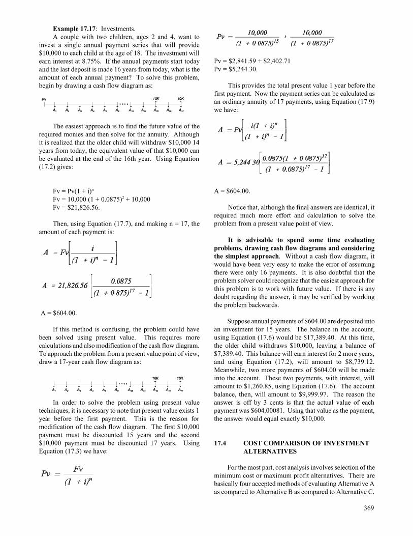
Example 17.17: Investments.A couple with two children, ages 2 and 4, want to
invest a single annual payment series that will provide$10,000 to each child at the age of 18. The investment willearn interest at 8.75%. If the annual payments start todayand the last deposit is made 16 years from today, what is theamount of each annual payment? To solve this problem,begin by drawing a cash flow diagram as:
The easiest approach is to find the future value of therequired monies and then solve for the annuity. Althoughit is realized that the older child will withdraw $10,000 14years from today, the equivalent value of that $10,000 canbe evaluated at the end of the 16th year. Using Equation(17.2) gives:
Fv = Pv(1 + i)n
Fv = 10,000 (1 + 0.0875)2 + 10,000Fv = $21,826.56.
Then, using Equation (17.7), and making n = 17, theamount of each payment is:
A = $604.00.
If this method is confusing, the problem could havebeen solved using present value. This requires morecalculations and also modification of the cash flow diagram.To approach the problem from a present value point of view,draw a 17-year cash flow diagram as:
In order to solve the problem using present valuetechniques, it is necessary to note that present value exists 1year before the first payment. This is the reason formodification of the cash flow diagram. The first $10,000payment must be discounted 15 years and the second$10,000 payment must be discounted 17 years. UsingEquation (17.3) we have:
Pv = $2,841.59 + $2,402.71Pv = $5,244.30.
This provides the total present value 1 year before thefirst payment. Now the payment series can be calculated asan ordinary annuity of 17 payments, using Equation (17.9)we have:
A = $604.00.
Notice that, although the final answers are identical, itrequired much more effort and calculation to solve theproblem from a present value point of view.
It is advisable to spend some time evaluatingproblems, drawing cash flow diagrams and consideringthe simplest approach. Without a cash flow diagram, itwould have been very easy to make the error of assumingthere were only 16 payments. It is also doubtful that theproblem solver could recognize that the easiest approach forthis problem is to work with future value. If there is anydoubt regarding the answer, it may be verified by workingthe problem backwards.
Suppose annual payments of $604.00 are deposited intoan investment for 15 years. The balance in the account,using Equation (17.6) would be $17,389.40. At this time,the older child withdraws $10,000, leaving a balance of$7,389.40. This balance will earn interest for 2 more years,and using Equation (17.2), will amount to $8,739.12.Meanwhile, two more payments of $604.00 will be madeinto the account. These two payments, with interest, willamount to $1,260.85, using Equation (17.6). The accountbalance, then, will amount to $9,999.97. The reason theanswer is off by 3 cents is that the actual value of eachpayment was $604.00081. Using that value as the payment,the answer would equal exactly $10,000.
17.4 COST COMPARISON OF INVESTMENTALTERNATIVES
For the most part, cost analysis involves selection of theminimum cost or maximum profit alternatives. There arebasically four accepted methods of evaluating Alternative Aas compared to Alternative B as compared to Alternative C.
369
17.4.1 Present Value Method
The first of these methods is the present valuetechnique, wherein all costs and revenues are discountedback to present value to arrive at a net present value for theproject. This method is very time consuming if performedmanually and presents problems when the alternatives havedifferent economic lives. Alternative A may have anexpected life of 10 years, Alternative B may have anexpected life of 15 years, and Alternative C may have anexpected life of 20 years. Therefore, in order to do anymeaningful evaluation of these three alternatives in terms ofpresent value, it is necessary to find a common denominatorfor their expected life, which, in this case, would be 60 years,where Alternative A would be replaced six times, B replacedfour times, and C replaced three times.
17.4.2 Future Value Technique
The future value technique of evaluating alternatives isalmost identical to the present value method except that allcosts and revenues are stated in terms of future value. Theproblem still arises of alternatives with incompatible usefullives. The above techniques are self-explanatory, andbecause they require such extensive calculations, they willnot be covered further. But, because they exist, whenevaluating alternatives using computers, it is convenient toindicate, somewhere in the output data generated, the netpresent value (NPV) of each alternative. Manyorganizations base their decisions on NPV, andgovernmental agencies, expect to evaluate benefit-cost ratios.The benefit-cost ratio is the ratio of benefits provided by thealternative versus cost incurred, and will be discussed laterin this chapter.
17.4.3 Annual Equivalent Cost Method
The annual equivalent cost method of evaluatingalternative projects states all costs and revenues overthe useful life of the project in terms of an equal annualpayment series (an ordinary annuity). This is probably themost widely used method in the industry, for several reasons:
1. It requires less effort and fewer calculations.
2. It eliminates the problem of alternatives withincompatible useful lives.
3. It allows for much more sophistication whenconsidering inflation, increasing equipment cost,equipment depreciation schedules, etc.
The annual cost method assumes that the project willlive forever, and that, if Alternative A has a useful life of 10years and Alternative B has a useful life of 15 years, eachalternative will be replaced at the end of its useful life.Therefore, the alternative with the minimum annual cost ormaximum annual profit is the alternative that will be chosen.
370
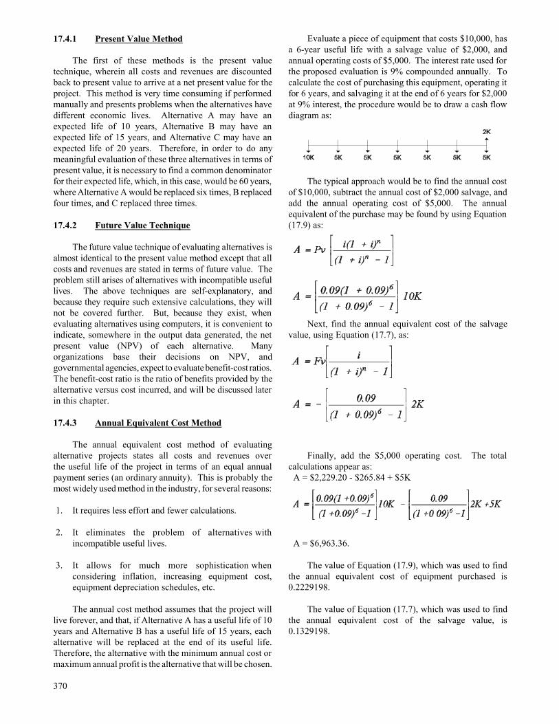
Evaluate a piece of equipment that costs $10,000, hasa 6-year useful life with a salvage value of $2,000, andannual operating costs of $5,000. The interest rate used forthe proposed evaluation is 9% compounded annually. Tocalculate the cost of purchasing this equipment, operating itfor 6 years, and salvaging it at the end of 6 years for $2,000at 9% interest, the procedure would be to draw a cash flowdiagram as:
The typical approach would be to find the annual costof $10,000, subtract the annual cost of $2,000 salvage, andadd the annual operating cost of $5,000. The annualequivalent of the purchase may be found by using Equation(17.9) as:
Next, find the annual equivalent cost of the salvagevalue, using Equation (17.7), as:
Finally, add the $5,000 operating cost. The totalcalculations appear as: A = $2,229.20 - $265.84 + $5K
A = $6,963.36.
The value of Equation (17.9), which was used to findthe annual equivalent cost of equipment purchased is0.2229198.
The value of Equation (17.7), which was used to findthe annual equivalent cost of the salvage value, is0.1329198.

Notice that the difference between 0.2229198 and0.1329198 is exactly equal to the interest rate (i), 0.09. Thisis true for all interest rates, provided that these functionshave the same i and the same n.
In calculating the annual equivalent cost of purchasingthe equipment and subtracting the annual equivalent cost ofthe equipment salvage at some time in the future, this isalways the case: i and n are equal; and Equation (17.9) - i= Equation (17.7).
Using functional notation as symbols for these formulaswe have:
[(A/P,9,6) - 0.09] = (A/F,9,6).
Making this substitution, the annual cost formulabecomes:
A = (A/P,9,6)10K - [(A/P,9,6) - 0.09]2K + 5K
multiplying,
A = (A/P,9,6)10K - (A/P,9,6)2K + 0.09(2K) + 5K
factoring out (A/P,9,6),
A = (A/P,9,6)(10K - 2K) + 0.09(2K) +5K
the general equation for the annual cost equation becomes:
then
A = (A/P,i,n)(cost - salvage) + i(salvage) + OC (17.14)
represents the annual equivalent cost formula
where
OC = annual operating cost.
This modification of the annual cost formula greatlyreduces the amount of calculation necessary to arrive at theannual equivalent cost.
Values can be produced by this formula as monthlyequivalent costs or weekly equivalent costs by simplychanging i to the interest rate per period and allowing n toequal the total number of periods. Using the previousexample, suppose the annual percentage rate was 9%compounded monthly. To calculate the periodic costs interms of monthly equivalent costs (as a monthly ordinaryannuity):
A = (A/P,0.75,72)(10K - 2K) + 0.0075(2K) + 5K/12A = $144.20 + $15.00 + $416.67A = $575.87.
Stating costs as an ordinary annuity has nothing to dowith actual cost flows. It simply states all costs and revenuesas an equal payment series in order that one alternative maybe compared with another (See Figure 17.2).
Figure 17.2 Annual Equivalent Cost.
371

17.4.4 Rate of Return Method
The rate of return (ROR) method of comparingalternatives calculates the interest rate for each alternativeand selects the highest ROR. A word of caution isnecessary, ROR evaluates INVESTED capital and the costsof operation and maintenance as opposed to revenues orbenefits received from the project. Therefore, a projecttotally financed with borrowed money has no rate of returnbecause there is no invested capital. The followingexamples assume 100% equity financing and are used toillustrate rate of return calculations.
Example 17.18: An investment of $7,000 is placedinto an account for a 10-year period. At the end of 10 years,the balance in the account is $17,699.30. What was theannual interest rate earned? Using Equation (17.2):
Fv = Pv(1 + i)n
$17,699.30 = $7,000(1 + i)10.
This problem can be solved by dividing both sides ofthe equation by $7,000 giving:
17,699.30/7,000 = (1 + i)10
2.528 = (1 + i)10.
Extracting the tenth root of each side of the equationgives:
(2.528)0.1 = [(1 + i)10]0.1
1.0972 = 1 + i
i = 0.0972.
A ROR can also be calculated by evaluating thedifference between alternatives that provide cost savingsrather than revenues.
Example 17.19: Fire insurance premiums on a ware-house are $500/y (Alternative A). The same coverage canbe purchased by paying a 3-year premium of $1,250(Alternative B). Find the ROR realized by purchasing a 3-year policy in place of three 1-year policies.
To simplify this problem, notice that the 3-yearinsurance premium is 2.5 times the annual premium. Thecash flow diagram for Alternative A appears below.
The cash flow diagram for Alternative B appearsbelow.
372
To further simplify this problem, consider thedifferences between these two alternatives. If Alternative Ais subtracted from Alternative B, the cash flow diagrambecomes:
Although the insurance premiums are an annuity due,the cash flow diagram above makes the cash flows appear asan investment of $1.5 providing an ordinary annuity of $1at the end of each year for 2 years. The analysis hassimplified the problem considerably and avoided using themore complex formulas associated with annuities due.Using Equation (17.8):
Entering values in this formula requires that themathematical signs be properly observed. If money flowingout, below the time line, is considered positive (+) thenmoney flowing in, above the time line, or money saved isconsidered negative (-). The calculation then becomes:
Notice there is one equation and one unknown (i), butthe unknown appears three times in the equation.Therefore, the only solution would be by an iterative
process. Continuing with Equation (17.8):
where
I = 0.21, or 21%Pv = 1.5A = - 1.
The answer to this problem is - 0.00946, indicatingthat the first interest rate was too low.
Try i = 22%
The answer, 0.00847, indicates the interest rate is toohigh. The actual interest rate is 21.525043%. Placing thisinterest rate into the formula for i, the answer equals zero,indicating that the ROR realized by purchasing a 3-year

policy instead of three 1-year policies is 21.5%. There aremany pocket calculators costing under $20 that are designedto calculate financial functions and are capable of iteratingfor problems involving a single financial function.
Consider the annual cost formula where:
a = (A/P,i,n) x ( cost - salvage) + (i) salvage + OC - revenues.
Suppose it is required to find the ROR on such aproject. Once again, the solution to the problem is found byiteration. But in this case, there is more than one financialfunction. Choose an interest rate. Work the problem at thatinterest rate, and find out if the answer comes out positive ornegative. With the mathematical signs we have used in thisexample, if revenues exceed costs the answer would benegative; if costs exceed revenues the answer would bepositive. When the exact i is placed into the formula thatdenotes the ROR, the answer would be zero. That is, theinterest rate that causes revenues and costs to be exactlyequal. Interest tables may be used to help find an upper andlower range for i to reduce the number of iterationsnecessary.
A much easier solution is to place all of the cash flowsby year into a computer and write a simple program that cando thousands of iterations in a matter of seconds to find i.
Trying to iterate i for a problem with more than onefunction on a financial calculator nearly always results inerror because of the tremendous amount of time and datathat must be entered by hand. Even with a computerprogram, if the cash flows turn from negative to positive andback to negative during the project life, i can take on theform of a quadratic equation and the computer is unable todetermine whether i is positive or negative. There arecomputer spreadsheets and other software available foriterating i, but these have their limitations. One of the mostpopular and widely used spread-sheets is designed to iteratei for a series of cash flows. However, this spreadsheetrequires a rather accurate guess for i; because, if it does notfind i after 20 iterations, the resultant answer is "Err"(error). The RELCOST program developed to accomplishLCC analysis (copyright, Washington State Energy Office)will iterate i to seven decimal places in a matter of secondsfor projects with over 150 input variables and more than 500inflation rates, and evaluate the iterated i to determinewhether it is positive or negative. This program will bediscussed in more detail in Subsection 17.7, entitled "LIFECYCLE COST ANALYSIS."
17.5 GRADIENTS
17.5.1 Arithmetic Gradients
Having developed formulas for equal payment seriesinvolving both ordinary annuities and annuities due, an end-of-period payment series that increases by a fixed dollar
amount at the end of each period can now be evaluated.Consider the following end-of-period payments:
As can be seen in the cash flow diagram above, thepayment series started at $100 and increased by $20 peryear. Such a payment series is called an arithmetic gradient.Although such a payment series is covered in detail by mosttexts on engineering economics, it is highly unlikely thatany portion of a project will contain such a payment series.
The method used to solve for present value, futurevalue or annual equivalent cost of such a payment series isto break it up into a series of ordinary annuities.
This payment series now appears as five ordinaryannuities. Because the series is progressing in the directionof future value, it is easiest to assume one annual paymentseries of $100 and find the future value of the sum of theremaining four annuities and string them out in the formof an annual equivalent for the 5-year period. The formulato accomplish this, where n = 5 and i = 9%, is:
The 5-year equivalent cost of an arithmetic gradient of$20 that begins at the end of year 2 and increases throughyear 5 is $36.56. Therefore, the annual equivalent of thepayment series that began with $100 and increased by $20for the next 4 years is $100 + $36.56, or $136.56.
Notice that when dealing with an arithmetic gradient,A1 becomes an ordinary annuity, and the amount of increasestarting at the end of the second period is considered to bethe gradient. The gradient formula is based on the fact thatthe gradient always begins at the end of the second periodand is to be strung out as an equal payment series from theend of the first period to the end of the cash flow. Thegeneral formula for finding the equivalent annual cost of anarithmetic gradient is:
(A/G,i,n)(17.15)
This is the arithmetic gradient uniform series factorwhere G is the amount of increase beginning at the end ofthe second period.
373

If the present value or future value of an arithmeticgradient is required, one could simply multiply Equation(17.15) by (P/A,i,n) or (F/A,i,n).
The most common use of arithmetic gradients is incalculating the value of sum-of-years-digits (S-Y-D)depreciation, which takes the form of a negative arithmeticgradient. This method of depreciation is no longer allowedunder the 1987 tax law.
17.5.2 Geometric Gradients
A geometric gradient is an end-of-period paymentseries that increases by a fixed percentage each period.Consider a 5-year payment series that begins with $100 andincreases by 9% every year thereafter. A cash flow diagramused for calculation of the problem is shown as:
The cash flow diagram above illustrates a geometricgradient with the first payment (A1) equal to $100 and eachsubsequent payment increasing by 9% in other words, a$100 payment inflating at a rate (g) of 9% annually. Then:
and the present value (Pv) for an assumed cost of capital of12% compounded annually (i) is:
Let n equal the number of interest periods (years, inthis case). Then:
374
Note that:
where g is constant.
Therefore:
Then, to find the annual equivalent cost (A),considering inflation: annual cost = present cost x capitalrecovery factor (A/P,i,n) and is written:
A = PV x (A/P,i,n)
Multiplying by the capital recovery factor:
Simplifying:
(A/A1,g,i,n) (17.16)
where g does not equal i.
This is the geometric gradient uniform series factor,where g does not equal i.
Using functional notation:

Inserting the initial values in this example:
(0.2774) = $117.38.
The annual equivalent cost equals $117.38. Figure17.3, plots a geometric gradient increasing by 9% for 20years and indicates the annual equivalent cost at a discountrate of 12%.
Notice, by removing the capital recovery factor inEquation (17.16), the equation becomes:
(P/A,g,i,n)(17.17)
where g is not = i.
This is the geometric gradient present worth factor,where g is not = i.
In the case where the discount rate equals the rate ofinflation (g = i), the equation becomes A1 divided by zero,which is undefined. If a geometric gradient is increasing byexactly the discount rate, this has the same effect of aninterest rate equal to zero; therefore, simply take A1,multiply it by the total number of payments (n), which willyield a present value at the end of year one. Because presentvalue represents the dollar equivalent at time zero, theamount that was calculated by multiplying A1 by n is oneinterest period off. To bring it to the proper time frame,time zero, simply discount it by one time period. Therefore:
(P/A1,g,i,n) (17.18)
where g = i.
This is the geometric gradient present worth factor,where g = i.
Although geometric gradients are rather common andare found in many applications, they require that the rate ofincrease remain constant. Such is not the case in mostenergy forecasts, where inflation rates are modified year byyear. This problem will be discussed later in Section 17.7under the heading, "LIFE CYCLE COST ANALYSIS."
Figure 17.4 graphs a project with the following inputvariables:
20-year AnnualEquivalent Costs
Project life in years 20Interest rate (APR) 12%Capital investment $120,000 $16,065Salvage value 12,000 -167Annual costs
Insurance 500 560Fixed 2,250 2,250Arithmetic gradient 230 1,385Geometric gradient increasing at 10% 2,000 4,051 increasing at 6% 10,000 14,895
Depreciation method 200% declining balance
Figure 17.4 illustrates the total annual equivalent costsfor operating this project for 1 year, 2 years, 3 years, etc.The capital recovery line indicates the annual equivalent ofinvesting capital and salvaging the project at end of year 1,2, 3, etc. The operation and maintenance line shows theannual equivalent cost of operating the project in years 1through 20. Notice that the minimum annual cost occurs inyear 15, which is $38,486. That is to say, the annualequivalent stream of equal payments for operating theproject with a 15-year life would be $38,486/y.
Table 17.2 Economic Life Calculations________________________________________________
Capital O&M Total SalvageYear Recovery Costs Costs Values 1 $38,400 $14,810 $53,210 $96,000 2 34,777 15,296 50,073 76,800 3 31,754 15,779 47,533 61,440 4 29,224 16,259 45,483 49,152 5 27,100 16,735 43,834 39,322 6 25,311 17,207 42,517 31,457 7 23,800 17,674 41,473 25,166 8 22,519 18,135 40,655 20,133 9 21,431 18,592 40,023 16,106 10 20,554 19,042 39,596 12,000 11 19,629 19,485 39,114 12,000 12 18,875 19,922 38,797 12,000 13 18,253 20,352 38,605 12,000 14 17,734 20,774 38,509 12,000 15 17,297 21,189 38,486 12,000 16 16,926 21,596 38,522 12,000 17 16,609 21,995 38,604 12,000 18 16,337 22,385 38,722 12,000_____________________________________________
375

Years
2 4 6 8 10 12 14 16 18 20
3
5
4
6
4
2
7
8
9
Actual cash flow
Annual equivalent cost @12%
10
20
30
40
50
60
DO
LLA
RS
(Tho
usan
ds)
2 4 6 8 10 12 14 16 18 20YEARS
Capital Recovery
Total Annual Cost
O & M
Figure 17.3 Geometric gradient.
Figure 17.4 Economic life.
376

Table 17.2 provides annual equivalent values from year1 through year 18 for capital recovery, operation andmaintenance costs, and total annual costs. Salvage valuesfor any given year are indicated in the last column. Thisanalysis is beyond the scope of this chapter, but could beused to determine the economic life (minimum annual cost)of a project that had these cost characteristics. Table 17.2provides answers for various costs that could be beneficial tothose who want to sharpen their expertise in calculatingcapital recovery, annuities due, ordinary annuities,geometric gradients, and arithmetic gradients.
17.6 EQUIPMENT DEPRECIATION
A discussion of equipment depreciation is essential inevaluating projects for taxable entities because equipmentdepreciation significantly lowers the annual cost of a project.This subject is also the area of constant change because itchanges as tax laws are revised. The amount of total capitalinvestment in a project and the reduction in tax liabilitycaused by depreciation or investment and energy tax creditsor both, all have a major bearing on whether or not theproject is economically feasible. However, the 1986 tax lawdrastically reduced many of these incentives. Competent taxaccountants should be a part of the development team toensure proper utilization of these considerations.
17.6.1 Straight Line Depreciation
Straight line depreciation is the simplest form ofdepreciation and has survived tax law changes for manydecades and it is accepted by the 1987 tax law. The formulafor straight line depreciation is:
Life can be expressed in years, months, units ofproduction, operating hours, or miles. Under the 1987 taxlaw, salvage values are set to zero.
17.6.2 Sum-of-Years Digits Depreciation
This depreciation method is an accelerated depreciationschedule that recovers larger amounts of depreciation in theearly life of the asset. The method of calculation is asfollows:
1. Find the sum of the years' digits of the life of theequipment. Example: For a 10-year life, the sum ofthe digits 1 through 10 is equal to 55. The easiest wayto make this calculation is:
in this case,
2. This sum is then divided into cost minus salvage toobtain one unit of depreciation, which is:
Example: Equipment cost = $60,000 Salvage value = $ 5,000
then,
3. This unit of depreciation is then multiplied by the years
of life in descending order, that is:
year 1 = 10 units = $10,000year 2 = 9 units = $ 9,000year 3 = 8 units = $ 8,000------ -- -- --------- -- --------- year 10 = 1 unit = $ 1,000.
The depreciation charge under this method performslike a negative arithmetic gradient where A1 is$10,000 and G is -$1,000.
Although this method of depreciation is acceptedaccounting practice and may be used on equipmentpurchased before 1980, it is no longer allowed underthe 1987 tax law and is only discussed to illustrate anapplication of the arithmetic gradient.
17.6.3 Declining Balance Depreciation
This method of depreciation is also an accelerated formand may obtain even larger depreciation in the early lifethan S-Y-D. With 200% declining balance depreciation, theannual rate is 200% times the straight line rate. As anexample:
An asset with a 10-year life has a straight line rate of1/10. Therefore, the 200% declining balance ratewould be 2/10 or 20%.
This rate is applied to the book value of the asset,where book value equals cost minus accumulateddepreciation. Any salvage value of the equipment wasnot considered except that the tax code provided thatthe equipment could not be depreciated below itssalvage value. The $60,000 piece of equipment in theexample above would be evaluated using 200%declining balance as shown in Table 17.3.
377

Table 17.3 Declining Balance Depreciation Using200% Declining Balance
________________________________________________ Book Value x Annual Book ValueDepreciation Rate Depreciation End of Year
Year ($) ($) ($) 1 60,000 x 0.20 12,000 48,000 2 48,000 x 0.20 9,600 38,400 3 38,400 x 0.20 7,680 30,720 - - -________________________________________________
Although this method of depreciation provides themaximum write-off in the early life of the equipment, theannual depreciation charge rapidly decreases to the pointthat it would be beneficial to switch to straight line after the6th year. It is interesting to note that the declining balancemethod of depreciation, whether it be 200%, 150% or 125%,takes the form of a negative geometric gradient and the bookvalue for any year can be calculated using Equation (17.2).In this example,
Fv = $60,000 (1 - 0.20)3
Fv = $30,720 = book value end of year 3,
to calculate the depreciation for year 6,
Fv = [60,000 (1 - 0.205)] 0.20Fv = $3,932,16.
In the example above, the book value is calculated forthe end of year 5, and multiplied by the depreciation rate,0.20, to obtain the annual depreciation for year 6.
Once again, although this method of depreciation is anaccepted accounting method, declining balancedepreciation was made obsolete with the 1980 tax lawchanges. However, a modified version of this method wasreinstated with the 1986 tax code revision and is discussedbelow.
17.6.4 Modified Accelerated Cost Recovery System(MACRS)
The Accelerated Cost Recovery System (ACRS) wasintroduced in 1981, but underwent major revision in 1986,effective with the 1987 tax year. In 1989, the ModifiedAccelerated Cost Recovery System (MACRS) wasintroduced, which was another major revision. MACRSdepreciation is designed to provide rapid depreciation and toeliminate disputes over depreciation methods, useful life,and salvage value. The depreciation method and useful lifeare fixed by law, and the salvage value is treated as zero.MACRS depreciation rates depend on the recovery period
378
for the property and whether the mid-year or mid-quarterconvention applies. Property with class lives of 3, 5, 7, and10 years may be depreciated at either the 200% or the 150%declining balance rate, with a switch to straight line.Property with class lives of 15 and 20 years must bedepreciated using the 150% declining balance rate with aswitch to straight line. In either case, the switch to straightline occurs when the straight line rate provides largerannual deductions. Table 17.4 lists the various classes ofdepreciable property under the Modified Accelerated CostRecovery System.
Table 17.4 MACRS Class Lives________________________________________________
Property All personal property other than real estate.Class________________________________________________
Special handling devices used in themanufacturing of food and beverages.
3-Year Special tools and devices used in the manu-Property facture of rubber products, fabricated metal
products, or motor vehicles, and finished plasticproducts.
Property with a class life of 4 years or less.
________________________________________________Automobiles, light-duty trucks (unloaded weightof less than 13,000 pounds).
Semi-conductor manufacturing equipment.
Aircraft owned by non-air transport companies
Typewriters, copiers, duplicating equipment,heavy general purpose trucks, trailers, cargocontainers, and trailer mounted containers.
Computers.
5-Year Computer-based telephone central officeProperty switching equipment, computer-related
Peripheral equipment, and property used inresearch and experimentation.
Equipment qualifying as a small powerproduction facility within the meaning of Section3(17)(C) of the Federal Power Act (16 U.S.C.796 (17)(C)), as in effect on 9-1-86.
Petroleum drilling equipment.
Property with a class life of more than 4 and lessthan 10 years.
________________________________________________

Table 17.4 MACRS Class Lives (continued)________________________________________________
Property All personal property other than real estate.Class______________________________________________
All property not assigned by law to anotherclass.
Any railroad track.
7-Year Office furniture, equipment, and fixtures. Property Cellular phones, fax machines, refrigerators,
dishwashers. Machines used to producejewelry, toys, musical instruments, andsporting goods.
Single-purpose agricultural or horticulturalstructures placed in service in 1987 or 1988.
Property with a class life of 10 years or more,but less than 16 years.
_______________________________________________Equipment used in the refining of petroleum,the manufacture of tobacco products andcertain food products.
Railroad cars.10-YearProperty Water transportation equipment and vessels.
Single-purpose agricultural or horticulturalstructures place in service after 1988.
Property with a class life of 16 years or more,but less than 20 years.
________________________________________________Land improvements such as fences, shrubbery,roads, and bridges.
Any municipal waste water treatment plant.
15-Year Telephone distribution plants and equipmentProperty used for 2-way exchange of voice and data
communications.
Property with a class life of 20 years or more,but less than 25 years.
________________________________________________Farm buildings.
20-Year Municipal sewers.Property
Property with a class life of 25 years or more.________________________________________________27.5-Year Residential rental property (excluding hotels Property and motels) placed in service after December
31, 1986.________________________________________________31.5 Year Non-residential real property placed inProperty service after December 31, 1986, but before
May 13, 1993.________________________________________________39-Year Non-residential property placed in serviceProperty after May 12, 1993.________________________________________________
The mid-year convention treats all property acquiredduring the year as though it were acquired in mid-year andonly half of the first year depreciation is allowed. Similarly,in the year after the last class life year, the remainingdepreciation is written off. If property is sold, only half ofthe full depreciation for the year of sale is allowed.Therefore, if the $60,000 piece of equipment is depreciatedunder MACRS, the depreciation schedule would be asshown in Table 17.5
Table 17.5 Depreciation Schedule________________________________________________
Book Value x Annual Book ValueDepreciation Rate Depreciation End of
YearYear ($) ($) ($) 1 60,000 x 0.10 6,000 54,000 2 54,000 x 0.20 10,800 43,200 3 43,200 x 0.20 8,640 34,560 -- -- --__________________________________________________
Under this system of depreciation, the user wouldswitch to straight line in year 7. Table 17.6 provides valuesfor the various classes of equipment and these values switchto straight line automatically in the year that straight linewill provide a larger annual depreciation. In year 7, 8, 9,and 10, the depreciation on the $60,000 piece of equipmentwould be $3,900/year. However, in year 11, which isconsidered the year of disposal (for tax purposes), the mid-year convention would allow only $1,965 of depreciation.
Table 17.6 provides depreciation percentage values forModified Accelerated Cost Recovery System using the mid-year convention.
Figure 17.5 illustrates an asset costing $50,000 withzero salvage value and a 10-year life depreciated by all ofthe above methods.
During years 7 through 10, MACRS and 200%declining balance are almost identical. The property is fullydepreciated at the end of year 10 using 200% decliningbalance; but, using MACRS, the mid-year conventionapplies in year 11.
The mid-quarter convention applies when more than40% of all property placed in service during the year isacquired during the last three months of the year. Under themid-quarter convention, property placed in service in anyquarter is treated as though it were acquired in mid-quarterand only half of the depreciation for that quarter is allowed.That is, property acquired in the first quarter would beallowed 3.5 quarters of depreciation in the first year.Property acquired in the third quarter would be allowed 1.5
379

Years
0 1 2
200% DB
4 5 6 7 8 9 10 110
1
2
3
4
5
6
8
7
9
10
3
MACRS
S-Y-D
Straight line
MACRS
MACRS
Table 17.6 MACRS Depreciation Values Mid-YearConvention
________________________________________________ 3- 5- 7- 10- 15- 20-
Recovery Year Year Year Year Year Year Year Class Class Class Class Class Class
1 33.33% 20.00% 14.29% 10.00% 5.00% 3.75% 2 44.44 32.00 24.49 18.00 9.50 7.22 3 14.81 19.20 17.49 14.40 8.55 6.68 4 7.41 11.52 12.49 11.52 7.70 6.18 5 11.52 8.92 9.22 6.93 5.71 6 5.76 8.92 7.37 6.23 5.28 7 8.92 6.55 5.90 4.89 8 4.46 6.55 5.90 4.52 9 6.55 5.90 4.4610 6.55 5.90 4.4611 3.28 5.90 4.4612 5.90 4.4613 5.90 4.4614 5.90 4.4615 5.90 4.4616 2.95 4.4617 4.4618 4.4619 4.4620 4.4621 2.23
__________________Notes: The table values are to be multiplied by the cost basis of the
equipment.
3-year class through 10-year class is depreciated using 200%declining rate, converting to straight line in the year underlined.
15- and 20-year class property is depreciated using the 150%declining rate converting to straight line in the year underlined.
The half-year convention treats all classes as though they wereplaced in service in mid-year, allowing 0.5 y of depreciation in year1 and 0.5 y of depreciation when the property is disposed of,removed from service, or in the last recovery year.
____________________________________________________
quarters of depreciation in the first year. Similarly, in theyear after the last class life year, the remaining quarters ofdepreciation are written off.
Mid-quarter values to multiply by the cost basis of theproperty may be calculated as follows:
Let remaining value (rv) = (1 - accumulated depreciation)Let remaining periods (rp) = (1 - accumulated periods)
then:
v = the greater of [(r/1)(rv)(np) or (rv/rp)(np)].
where,
v = the percentage value to multiple by the cost basisr = either 200% or 150% declining balance ratel = Property Class Life in terms of years or quartersnp = the number of periods allowed in the current yearrv = the remaining property valuerp = the remaining periods.
Example: 17.20: MACRS Mid-Quarter Convention.Property with a class life of 5 years, purchased
during the second quarter, is to be depreciated by the mid-quarter convention, using the 200% Declining Balance Rate.Values to be multipled by the cost basis of the equipmentcould be generated using the above formulas as follows:
Figure 17.5 Depreciation methods.380

Declining Straight Periods Remaining Value Balance Line Allowed Value | Periods
Year (m) (r/l)(rv)(np) (rv/rp)(np) (np) (rv) (rp) 1 25.00% 25.00% 12.50% 2.5 100.00% 20.0 2 30.00 30.00 17.14 4 75.00 17.5 3 18.00 18.00 13.33 4 45.00 13.5 4 11.37 10.80 11.37 4 27.00 9.5 5 11.37 6.25 11.37 4 15.63 5.5 6 4.26 0.64 4.26 1.5 4.26 1.5
The underlined values are multiplied by the cost basisof the property to determine the amount of depreciationallowed in each respective year.
The Internal Revenue Code also provides for first-yearexpensing of equipment placed in service in 1997. Thefirst-year expensing is technically called the “Section 179Deduction.” The deduction is limited to $18,000 in 1997and will increase in 1998. The deduction phases out whenequipment costing over $200,000 is placed in service in anyone year. The deduction is not allowed for buildings,structural components of buildings, and furnishings ofresidential rental property. First-year expensing must besubtracted from the cost basis of the equipment fordepreciation purposes.
The Internal Revenue Code and the annual changesthat occur are beyond the scope of this text. Users mustmaintain current knowledge of the tax law in order to becertain they are in compliance with existing guidelines.
17.7 LIFE CYCLE COST ANALYSIS
Life cycle costing (LCC) evaluates all the costsassociated with acquisition, construction and operation of aproject. LCC is designed to minimize costs of majorprojects, not only in consideration of acquisition andconstruction, but especially in the reduction of operation andmaintenance costs during the project life. LCC is thecalculation of all annual costs and revenues over the life ofthe project. These values are totaled by year and discountedback to time zero at some interest rate to arrive at a netpresent value. This process is repeated for each alternative.The alternatives are then compared, based on net presentvalue or equivalent annual cost.
When performing this analysis, it is important to dosensitivity analysis. Sensitivity analysis consists ofchanging parameters or variables within the project todetermine their effect on the feasibility of the project.Sensitivity analysis is accomplished by substituting one typeof construction for another or evaluating various pieces ofequipment with different operating costs, evaluating whateffect a change in the economic inflation rate would have onthe project, and considering various financing scenarios toobserve their effect on the outcome.
Example 17.21: Table 17.7 provides the input data forevaluating three heating systems. As a very simple example
of LCC, consider a 15-year LCC for three alternatives (A,B, and C as shown in Tables 17.8, 17.9, 17.10, 17.11,17.12, and 17.13) to provide heat for a 30,000 ft2 officebuilding.
Table 17.7 Heating System Cost Alternatives________________________________________________
Electric Heating Resistance Heat Pump Geothermal
Capital cost ($) 158,400 180,000 233,100Life (y) 12 12 12Salvage value ($) -0- -0- -0-Annual electricity requirement (kWh) 263,680 131,840 22,620Cost ($/kWh) $ 0.05 $ 0.05 $ 0.05Annual maintenance ($) 1,584 2,650 2,331Annual insurance ($) 554 630 816Annual property tax ($) 238 270 350Compressor replacement end of year 10 ($) -0- 750 -0-________________________________________________
Tables 17.8, 17.9, and 17.10 provide a 15-year LCC oneach system by year and evaluate these costs at 8% com-pounded annually. Electrical power costs are assumed to be$0.05/kWh. Notice each cost is entered in the year itoccurs. Insurance premiums are paid annually and are inthe form of an annuity due. Based on the present value atan 8% rate of interest over the 15-year life cycle, the heatpump has the lowest cost, and based on the criteria of thelowest present value, the heat pump would be the bestselection. However, when the cost of electricity is increasedto $0.07/kWh, presented in Tables 17.11 and 17.12, thegeothermal system becomes less expensive, having a lowernet present value, and lower annual equivalent costs.
Although the annual equivalent cost accuratelyindicates which alternative is the best choice, it hasabsolutely nothing to do with actual expenditures per year.Although the Heat Pump costs $6,592/y to operate and hashigher maintenance costs than the Geothermal system, at$0.05/kWh it provides the lowest annual cost. The reasonfor this is the lower initial cost of the Heat Pump.
Another approach to LCC analysis would be toexamine the difference in costs between System B andSystem C. Table 17.13 illustrates this approach. Note thatthe cost of electricity has been changed to $0.07/kWh.Although $53,100 additional is spent by purchasing SystemC over System B, the net present value of the operatingcosts over a 15-year period at 8%/y is $13,019 more forSystem B than for System C. Because the savings inoperation and maintenance costs exceed the value of theinitial investment, System C would be chosen over SystemB.
381

Table 17.8 Life Cycle Cost of Heating System (A)________________________________________________
Electric Resistance HeatCapital Cost $158,400Interest Rate 8%Electric Power Cost $0.05/kWh
Electric Prop. Annual Power Ins. Tax Maint. Total Present
Cost Cost Cost Cost Cost ValueYear ($) ($) ($) ($) ($) ($) 0 -0- 554 -0- -0- 158,954 158,954 1 13,184 554 238 1,584 15,560 14,407 2 13,184 554 238 1,584 15,560 13,340 3 13,184 554 238 1,584 15,560 12,352 4 13,184 554 238 1,584 15,560 11,437 5 13,184 554 238 1,584 15,560 10,590 6 13,184 554 238 1,584 15,560 9,805 7 13,184 554 238 1,584 15,560 9,079 8 13,184 554 238 1,584 15,560 8,407 9 13,184 554 238 1,584 15,560 7,784 10 13,184 554 238 1,584 15,560 7,207 11 13,184 554 238 1,584 15,560 6,673 12 13,184 554 238 1,584 15,560 6,179 13 13,184 554 238 1,584 15,560 5,721 14 13,184 554 238 1,584 15,560 5,298 15 13,184 -0- 238 1,584 15,006 4,730
Total Cost $ 391,800Net Present Value $ 291,965
Annual Equivalent Cost $ 34,110
Table 17.9 Life Cycle Cost of Heating System (B)________________________________________________
Air-to-Air Heat PumpCapital Cost $180,000Interest Rate 8%Electric Power Cost $0.05/kWh
Electric Prop. Annual Power Ins. Tax Maint. Total Present
Cost Cost Cost Cost Cost ValueYear ($) ($) ($) ($) ($) ($) 0 -0- 630 -0- -0- 180,630 180,630 1 6,592 630 270 2,650 10,142 9,391 2 6,592 630 270 2,650 10,142 8,695 3 6,592 630 270 2,650 10.142 8,051 4 6,592 630 270 2,650 10,142 7,455 5 6,592 630 279 2,650 10,142 6,902 6 6,592 630 270 2,650 10,142 6,391 7 6,592 630 270 2,650 10,142 5,918 8 6,592 630 270 2,650 10,142 5,479 9 6,592 630 270 2,650 10,142 5,074 10 6,592 630 270 3,400a 10,142 5,045 11 6,592 630 270 2,650 10,142 4,350 12 6,592 630 270 2,650 10,142 4,028 13 6,592 630 270 2,650 10,142 3,729 14 6,592 630 270 2,650 10,142 3,453 15 6,592 -0- 270 2,650 9,512 2,999
Total Cost $ 332,880Net Present Value $ 267,589Annual Equivalent Cost $ 31,262
__________a. Indicates compressor replacement.
382
Table 17.10 Life Cycle Cost of Heating System (C)________________________________________________
Geothermal Heating SystemCapital Cost $233,100Interest Rate 8%Electric Power Cost $0.05/kWh
Electric Prop. Annual Power Ins. Tax Maint. Total Present
Cost Cost Cost Cost Cost ValueYear ($) ($) ($) ($) ($) ($) 0 -0- 816 -0- -0- 233,916 233,916 1 1,131 816 350 2,331 4,628 4,285 2 1,131 816 350 2,331 4,628 3,967 3 1,131 816 350 2,331 4,628 3,673 4 1,131 816 350 2,331 4,628 3,401 5 1,131 816 350 2,331 4,628 3,149 6 1,131 816 350 2,331 4,628 2,916 7 1,131 816 350 2,331 4,628 2,700 8 1,131 816 350 2,331 4,628 2,500 9 1,131 816 350 2,331 4,628 2,315 10 1,131 816 350 2,331 4,628 2,143 11 1,131 816 350 2,331 4,628 1,985 12 1,131 816 350 2,331 4,628 1,838 13 1,131 816 350 2,331 4,628 1,702 14 1,131 816 350 2,331 4,628 1,575 15 1,131 816 350 2,331 3,812 1,202
Total Cost $ 302,513Net Present Value $ 273,268
Annual Equivalent Cost $ 31,962
Table 17.11 Life Cycle Cost of Heating System (B)________________________________________________
Air-to-Air Heat PumpCapital Cost $180,000Interest Rate 8%Electric Power Cost $0.07/kWh
Electric Prop. Annual Power Ins. Tax Maint. Total Present
Cost Cost Cost Cost Cost ValueYear ($) ($) ($) ($) ($) ($) 0 -0- 630 -0- -0- 180,630 180,630 1 9,229 630 270 2,650 12,779 11,832 2 9.229 630 270 2,650 12,779 10,956 3 9,229 630 270 2,650 12,779 10,144 4 9,229 630 270 2,650 12,779 9,393 5 9,229 630 270 2,650 12,779 8,697 6 9,229 630 270 2,650 12,779 8,053 7 9,229 630 270 2,650 12,779 7,456 8 9,229 630 270 2,650 12,779 6,904 9 9,229 630 270 2,650 12,779 6,393 10 9,229 630 270 3,400a 12,779 6,266 11 9,229 630 270 2,650 12,779 5,481 12 9,229 630 270 2,650 12,779 5,075 13 9,229 630 270 2,650 12,779 4,699 14 9,229 630 270 2,650 12,779 4,351 15 9,229 630 270 2,650 12,149 3,830
Total Cost $ 372,432Net Present Value $ 290,159Annual Equivalent Cost $ 33,899
____________a. Indicates compressor replacement.

Table 17.12 Life Cycle Cost of Heating System (C)________________________________________________
Geothermal Heating SystemCapital Cost $233,100Interest Rate 8%Electric Power Cost $0.07/kWh
Electric Prop. Annual Power Ins. Tax Maint. Total Present
Cost Cost Cost Cost Cost ValueYear ($) ($) ($) ($) ($) ($) 0 -0- 816 -0- -0- 233,916 233,916 1 1,583 816 350 2,331 5,080 4,704 2 1,583 816 350 2,331 5,080 4,355 3 1,583 816 350 2,331 5,080 4,033 4 1,583 816 350 2,331 5,080 3,734 5 1,583 816 350 2,331 5,080 3,457 6 1,583 816 350 2,331 5,080 3,201 7 1,583 816 350 2,331 5,080 2,964 8 1,583 816 350 2,331 5,080 2,745 9 1,583 816 350 2,331 5,080 2,541 10 1,583 816 350 2,331 5,080 2,353 11 1,583 816 350 2,331 5,080 2,179 12 1,583 816 350 2,331 5,080 2,017 13 1,583 816 350 2,331 5,080 1,868 14 1,583 816 350 2,331 5,080 1,730 15 1,583 816 350 2,331 4,264 1,344
Total Cost $ 309,299Net Present Value $ 277,140
Annual Equivalent Cost $ 32,378
Another method of evaluation involves calculating theROR of the savings versus the costs. This method is alsoillustrated in Table 17.13. By iteration (trial and error), arate of 11.7986% causes the net present value of the savingsto be exactly equal to the net present value of the costs.Therefore, the ROR realized by selecting System C overSystem B is approximately 12% annually. Often in this typeof analysis, the actual annual costs are not an equal streamof payments, and may frequently swing from positive tonegative. Such detailed analysis on uneven cash flows canonly be performed efficiently with a computer program.
Tables 17.8 through 17.13 do not contain any form ofa gradient. If any of the costs are allowed to inflate, theproblem would become much more complex. Furthermore,all costs would not inflate at the same rate. The price of areplacement system 15 years from today would inflate at onerate, electricity at a different rate, and insurance wouldprobably be a different rate. However, with the use of amicrocomputer it would be possible to establish differentinflation rates for all cost data and perform the sameanalysis as shown in Tables 17.8 through 17.13.
These three alternatives are extremely sensitive to thecost of electrical power.
Table 17.13 Incremental Difference of System (C-B)________________________________________________
Geothermal minus Heat PumpIncremental Cost $ 53,100Interest Rate 8%Electric Power Cost $0.07/kWh
Electric Prop. Annual Power Ins. Tax Maint. Total Present
Cost Cost Cost Cost Cost ValueYear ($) ($) ($) ($) ($) ($) 0 -0- 816 -0- -0- -53,286 -53,286 1 7,645 186 80 319 7,699 7,129 2 7,645 186 80 319 7,699 6,601 3 7,645 186 80 319 7,699 6,112 4 7,645 186 80 319 7,699 5,659 5 7,645 186 80 319 7,699 5,240 6 7,645 186 80 319 7,699 4,852 7 7,645 186 80 319 7,699 4,492 8 7,645 186 80 319 7,699 4,159 9 7,645 186 80 319 7,699 3,851 10 7,645 186 80 1,069 8,449 3,913 11 7,645 186 80 319 7,699 3,302 12 7,645 186 80 319 7,699 3,057 13 7,645 186 80 319 7,699 2,831 14 7,645 186 80 319 7,699 2,621 15 7,645 -0- 80 319 7,699 2,486
Total Cost $ 63,134Net Present Value $ 13,019Annual Equivalent Cost $ 1,521Incremental Rate of Return on System © 11.7986%
__________________________________________________
17.8 RELCOST PROGRAM
LCC on a major project requires thousands ofcalculations involving every formula presented thus far inthis chapter with the possible exception of arithmeticgradients. However, with the advent of the microcomputerand software designed to do preliminary LCC analysis, thecost analyst can provide a relatively good guess as to theeconomic feasibility of a project.
The Renewable Energy Life Cycle COST program,RELCOST, was designed for just this purpose. Any LCCanalysis of a project requires an extensive accompanyingreport in order to explain in detail how values werecalculated. RELCOST provides an output, at the option ofthe user, that will print all of the input data, the energyforecast, the depreciation schedule, and all of the outputdata in tabular form, minimizing the need for anaccompanying report. RELCOST also provides an outputfile accessible to Harvard Graphics.
The program was developed through the WashingtonState Energy Office using funds provided by the state energyoffices of Washington and Oregon, and from private
383
sources. The 150 page user manual is supplied on a floppydisk. To obtain copies of this program, contact theWashington State University Energy Program, PO Box43165, Olympia, WA 98504-3165, telephone: 360-956-2016.
The RELCOST Program, Release 2.1, canaccommodate inflation rates for 13 different energies, and itis possible to change the inflation rate for each of theseenergies every year throughout an energy forecast of up to30 years. In addition, RELCOST will accommodate up tofive different classes of equipment with varying useful livesand with different depreciation schedules. Inflation ratesregarding equipment replacement can vary for eachequipment class.
RELCOST allows up to 5 years for construction andacquisition. During this construction period, it allows anycombination of project financing to include bonds, bankloans, and equity. It also allows capital investment duringthe construction period for project funds that are in excessof project costs for any particular year. The life of bankloans and bond issues can vary year by year, and interestrates may differ for bonds, bank loans, and investments foreach year of construction. The program permits 12 differentdepreciation schedules for equipment, including the half-year convention, and these rates may be altered by the user.The program makes provisions for percentage depletionallowances, investment tax credits, and energy tax credits.It can accept up to three annual revenue streams, inflatingat some user-defined rate per year over the life of the project.It also allows for a growth rate in the number of customerson-line in any given year.
RELCOST provides for four resident energy forecasts,up to 30 years in length. Once all the input data has beencollected, and energy forecasts have been established, theprogram requires less than 30 minutes to enter the data anddo the calculations for a major project.
A complete run on a hypothetical heating district for ataxable entity is provided in Tables 17.14 thru 17.22. Thesame project for a non-taxable entity appears in Tables17.23 thru 17.29.
The typical life-cycle cost input data supplied considersthe difference between an existing system and a proposedsystem; the same type of analysis that was performed usingSystem B and System C in Table 17.13. That is, theprogram considers the initial cost of the proposed systemand evaluates the annual savings provided by the proposedsystem versus the capital investment required for theproposed system to determine whether or not the system iseconomically feasible. It is not necessary to have a presentsystem. LCC analysis could be accomplished on a proposedsystem only. However, in order to perform this analysis, theprogram would have to consider the initial cost of theproposed system versus the revenues generated by theproposed system.
384
Table 17.14 illustrates input screen one, two, and threeof the RELCOST Program. Screen one consists of thereport title, location, date, and gives the user the option ofchoosing one of four forecast files or creating an energyforecast for this report only. These forecast files must becreated, maintained, and updated by the user.
Screen two begins with capital investment data. Dataentered on this sheet includes the beginning year of invest-ment, construction period, economic inflation rate, discountrate or cost of capital selected for the project and allfinancing data in the form of owner's equity, bonds, andbank loans used to finance the project.
Input screen three, which appears in the lower third ofTable 17.14, includes all present costs of energy for the exis-ting and the proposed system. The first five energies:natural gas, fuel oil, propane, coal, and electricity, are theconventional fuels supplied for every project. The next fiveenergies included under the heading Other Energy" are userselectable. The titles of these fuels are obtained from theenergy forecast. If no titles are supplied by the user, thenthey are listed as "Other 1" through "Other 5." The usermay elect to use any one or all of these fuels in the projectunder study.
The last two items on screen three: property tax andinsurance, and operation and maintenance, have their ownindependent inflation rates that are not in addition to theeconomic inflation rate. However, if the user wantedthese rates to inflate differently year by year, they could beentered on an energy forecast as an energy, properly titled,and these two items could be omitted at the bottom of screenthree.
Screen four Table 17.15 presents energy sales for boththe present and proposed systems. This screen also allowspercentages depletion allowance for energy sales under theproposed system. The amount of the percentage depletionallowance is determined by the user on the depreciationschedule under depletion, and if necessary, could changeyear by year, or as the tax code changes. The 1986 tax codechanged percentage depletion allowance from 20 to 22%,effective in 1987. The user must consult the current taxcode to determine those energies eligible for depletionallowance and the percent of depletion allowance. Theprogram does not provide cost depletion, although the usercould calculate such depletion in the depreciation section.Depletion allowances are only available for taxable entities.
Screen five on Table 17.15 presents five classes ofequipment. This screen allows the user to group allequipment associated with a project into five differentclasses depending upon economic life (the actual usable lifeof the equipment), taxable life, actual expected salvagevalue, taxable salvage value, and the method of depreciationto be applied against that class of equipment. This portionof the input section also allows inflation rates for subsequentpurchases of equipment and inflation rates for actual salvage

value to determine equipment replacement costs throughoutthe life cycle of the project. The user should be aware thatequipment is automatically replaced at the end of itseconomic life without any regard for the life of the project.In other words, if a class of equipment had a five-yeareconomic life, the project had a three-year constructionperiod and a life-cycle cost analysis was done for a 20-yearperiod, that class of equipment would auto-matically bereplaced at the beginning of year 9, 14, and 19.
There are 12 columns of depreciation schedulesavailable in the depreciation file. The data in these columnscan be modified by the user and hopefully will be adequatefor future changes to the tax law. Columns one through six,supplied with the program, provide ACRS depreciationschedules for 3-, 5-, 7-, 10-, 15-, and 20-year lives, using thehalf-year convention. The user may also select straight linedepreciation. Selecting this option will cause the programto calculate the annual depreciation charge for that class ofequipment based on its cost basis minus any salvage thatmay be allowed, for either a full-year or half-yearconvention, depending on the option selected by the user.All depreciation schedules are modifiable except for straightline.
Column zero supplies multipliers for percentagedepletion allowances.
The last screen on Table 17.15 is screen six, whichrequires income tax and investment tax credit input data.This screen allows the user to select the marginal federaland state tax rates, the percentage of investment tax creditor energy tax credit available or both, and the amount of thecapital investment eligible for these tax credits.
Table 17.16 is an example of a typical energy forecast.The inflation rates by year and by type of energy appear inthe columns as decimal amounts and represent an inflationrate above or below the economic inflation rate for each fuel.In other words, if the inflation rate in the natural gascolumn was 0.02 and the economic inflation rate was 0.06,this would indicate that natural gas was expected to inflateat 8% in year one. Inflation rates entered in the forecastmay be positive, negative or zero. A zero indicates that theenergy is expected to inflate at the same rate as theeconomic inflation rate.
Table 17.17 illustrates the depreciation and depletionallowance schedule. All values in these tables may bemodified by the user. However, the energy forecast islimited to 30 years. If the project life goes beyond 30 years,the inflation rate for year 30 is chosen as the inflation ratefor the last 10 years of the project.
Tables 17.18 through 17.22 provide the output data forthe project. Total project cost, equity financing and debtfinancing are all stated in terms of net present value; that is,all monies flowing into the project during the constructionperiod are brought back to time zero at the discount rate.
The benefit-cost ratio evaluates the net present value ofthe annual savings or revenues associated with the proposedsystem or both, and divides this number by the net presentvalue of the total project cost.
The net present value calculates the present value of thetotal project costs and subtracts the present value of theannual savings or revenues associated with the project orboth, to arrive at a net present value for the total project, ora net present value for the life cycle of the project.
A RELCOST user developed a scenario on a renewableenergy project with equipment that required replacementevery 6 months and he wished to evaluate this withequipment replaced every 18 months. In order toaccomplish this, all that was necessary was to statereplacement costs, all operating costs, all inflation rates, theeconomic inflation rate, capital investment costs andfinancing in terms of 1 month rather than 1 year,respectively, and complete a 36-month life cycle costanalysis. There are numerous ways to modify the input datain order to provide for unusual circumstances.
17.9 CAVEATS
As was stated in the introduction, LCC has severalmajor drawbacks. One of these is that increasing ordecreasing costs over the life of the project must beestimated based on some forecast, and forecasts have provento be highly variable and frequently inaccurate. Anotherproblem with LCC is that some life span must be selectedover which to evaluate the project, and many projects,especially renewable energy projects, are expected to havean unlimited life; they are expected to live forever. Thelonger the life cycle, the more inaccurate annual costsbecome because of the inability to forecast accurately.
Comprehensive LCC should be performed by qualifiedpersons who have a thorough knowledge of the subject,including expertise in the current tax law.
17.10 RECOMMENDATIONS
Based on the experience gained by the author incompleting over 150 economic analysis for renewableenergy projects, the following recommendations are offered.
17.10.1 Take the Time to Understand the Basics
Preliminary LCC requires that the user understandcertain basic concepts regarding interest, taxes, the timevalue of money, and economic decision techniques for eventhe simplest analysis. If you have no experience in theseareas, carefully read this chapter and proceed with extremecaution. If certain concepts remain unclear, consult thereferences appearing at the end of this chapter.
385
17.10.2 Use Ultraconservative Forecasts
During the petroleum crisis in the mid 1970s,forecasters were predicting inflation rates for fossil fuelsranging from 5 to 15% above the economic inflation rate.Many of these energy forecasts were 20 years in length.Using hindsight, it turns out that within the last 10 yearspetroleum prices have actually deflated when compared tothe consumer price index. Any forecast that projectsinflation rates higher than those that occur provides afavorable LCC picture, gives a green light to the project,causes thousands and even millions of dollars to be spent inacquisition and construction, only to find that when theproject goes into production, competing fuels have notinflated as projected and the project either operates at acontinual loss or is abandoned.
17.10.3 Keep Project Life as Short as Possible
It is dangerous to try to do even a 20-year study on amajor project. It is absolutely ridiculous to go beyond 20years. And yet, many projects have required 50-year LCCanalysis. The successful projects are those that useextremely low inflation rates and have a very short payback(4 years or less).
LCC analysis on a large project is a very complex pro-cedure. Many projects require equipment with widelyvarying useful lives. Pipe lines may last 25 years. Electricmotors, turbines, or pumps may have useful lives of 5 to 10years. Replacement costs must be forecast, major repaircosts have to be incorporated, and competing alternativesshould be as accurately evaluated as possible. If the projectis owned by a private entity, depreciation schedules,depletion allowances, investment tax credits, energy taxcredits, and in some cases, intangible drilling costs enter thepicture.
It is not possible to predict future changes in the taxlaw. In the early 1980s, many renewable energy projectsenjoyed as much as a 55% tax credit. Later (5 years), manyof these tax credits were removed. Therefore, anyequipment replaced could not provide the reduced taxliability that was forecast at the beginning of the project.
17.10.4 Minimize Total Project Cost
As observed in the LCC analysis of the three heatingsystems, initial cost probably has the greatest impact on thefeasibility of a project and the developer should make everyeffort to minimize the project cost without sacrificing qualityand reliability. For example, in the development of geother-mal projects, drilling costs, and pipeline costs are two of themajor components. In an attempt to minimize drilling costs,quality, performance and longevity of the production wellmay be sacrificed. It may be advisable to move the user on-site to minimize the length of transmission lines withoutsacrificing any other aspect of the project. The end result isa reduction of pipeline maintenance and pumping costs.
386
17.10.5 Carefully Evaluate Financing Options
The method of financing, the interest rate, and theannual debt service can have a major impact on renewableenergy projects. These projects are capital intensive andexperience very high costs during the construction period.In addition, many projects come on-line gradually, whichcauses very low revenues in the early years of the projectlife. In such cases, it may be advisable to seek long-termbond financing. Such financing requires only interestpayments during the early years of the project, and a highballoon payment when the bond matures. As the projectreaches full capacity in the later years, revenues may be ableto accommodate such a balloon payment. Such financingcan be especially helpful to municipalities experiencing lowor negative cash flows during the beginning years of theproject.
17.10.6 Avoid Distorting the Rate of Return
This author discourages using financial leverage tomake a project appear feasible. Financial leverage is thepractice of financing large sums of money at extremely lowinterest rates in order to reduce the equity invested in theproject and increase the ROR. For example, a projectcosting $100,000 returns $15,000 in revenues every year for10 years. The ROR on this project would be about 8%. Inan effort to make the project appear more attractive, thedeveloper borrows $90,000 at 6% interest, which requiresan annual payment of $12,228. Subtracting the debt servicefrom the income provides a net annual income of $2,772.Now, the project is evaluated as a $10,000 investmentproviding $2,772 of income per year for 10 years and theROR jumps to nearly 25%. Once project feasibility isdetermined, it is up to the developer to use any acceptedmethod to increase the project's ROR; but, such practicesshould be avoided in determining whether or not the projectis economically feasible.
17.10.7 Be Aware of the Limitations of Payback
Simple payback compares the values in the cumulativecash flow column (Table 17.22 column 22) with the equityinvested in the project to determine when these two valuesare equal. This practice makes no distinction betweenpresent and future values. Note that the simple paybackcash flows are not evaluated at any interest rate and that anegative cash flow occurring subsequent to the paybackperiod has no effect. If the cumulative cash flows indicatethat the equity in a project is recovered in year 12, and year13 has a balloon payment on a bond that causes the cashflow to turn negative, this may cause the simple payback tobe in error.
The discounted payback compares the equity in the pro-ject with the cumulative discounted cash flow (Table 17.22column 24) and indicates a discounted payback when thesetwo are equal. Once again, this method does not evaluatesubsequent negative cash flows that may occur.

Nonetheless, it is a more accurate measure of paybackbecause the accumulated cash flows are discounted at thediscount rate stated in the input section.
The reason the simple and discounted payback periodsare evaluated in this manner is because it is the acceptedcalculation method in the industry. Because these valuesmay be in error, the program RELCOST also evaluates cashflows beyond these payback periods and prints a warning inthe output section if negative cash flows occur beyond thepayback period.
The LCC analysis is a very powerful tool. It can beused to rank projects in the order of feasibility and todetermine which projects are most likely to be successful.At best however, it is only an educated guess and the valuescalculated should be treated only as rough estimates.
NOTE: See Glossary and References List at end of Chapter.
387
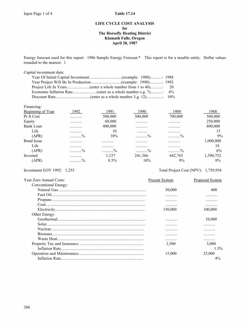
Input Page 1 of 4 Table 17.14
LIFE CYCLE COST ANALYSISfor
The Horsefly Heating DistrictKlamath Falls, Oregon
April 28, 1987
Energy forecast used for this report: 1986 Sample Energy Forecast.* This report is for a taxable entity. Dollar valuesrounded to the nearest: 1
Capital investment data:Year Of Initial Capital Investment...............................(example: 1988)...........: 1988Year Project Will Be In Production.............................(example: 1990)............: 1992Project Life In Years......................(enter a whole number from 1 to 40)...........: 20Economic Inflation Rate.......................(enter as a whole number e.g. 7)...........: 4%Discount Rate.................................(enter as a whole number 3.g. 12)...............: 10%
Financing:Beginning of Year 1992 1991 1990 1989 1988 Pr Jt Cost ........... 500,000 300,000 700,000 500,000Equity ........... 60,000 ........... ........... 250,000Bank Loan ........... 400,000 ........... ........... 800,000
Life ........... 10 .......... ........... 15(APR) ...........% 10% ...........% ...........% 9%
Bond Issue ........... ........... ........... ........... 1,000,000Life ........... ........... ........... ........... 18(APR) ...........% ...........% ...........% ...........% 6%
Invested ........... 1,157 241,366 642,765 1,390,752(APR) ...........% 8.5% 10% 9% 8%
Investment EOY 1992: 1,255 Total Project Cost (NPV): 1,759,954
Year Zero Annual Costs: Present System Proposed SystemConventional Energy:
Natural Gas.................................................................................. 50,000 400Fuel Oil........................................................................................ ........... ...........Propane....................................................................................... ........... ...........Coal............................................................................................. ........... ...........Electricity.................................................................................... 150,000 100,000
Other Energy:Geothermal.................................................................................. ........... 10,000Solar............................................................................................ ........... ...........Nuclear....................................................................................... ........... ...........Biomass...................................................................................... ........... ...........Waste Heat................................................................................. ........... ...........
Property Tax and Insurance............................................................. 2,500 3,000Inflation Rate.............................................................................. 1.5%
Operation and Maintenance............................................................. 15,000 25,000Inflation Rate............................................................................. 4%
388

Input Table 17.15Page 2 of 4
Year Zero Annual Costs: Present System Proposed System
Sales of Energy:Steam............................................................................................... ........... ...........Hot Water........................................................................................ ........... 220,000Tipping Fees................................................................................... ........... ...........
Percentage Depletion Allowance (for proposed system only):(See column 13 of Depreciation Schedule for rate.)
Indicate sales eligible Steam.............................................: Nofor percentage depletion Hot Water......................................: Yesallowance: (Y/N) Tipping Fees.................................: No
Taxable income limitations for depletion allowance.................................: 50%(Based on income resulting from sales eligible for depletion.)
Equipment Purchases: Class 1 Class 2 Class 3 Class 4 Class 5
Initial Cost: 500,000 250,000 120,000 90,000 ...........Yr. Purchased: 1988 1989 1990 1990 ...........Inflation/yr: 4% ..........% 5% ..........% 6%
Actual Slvg.: 50,000 .......... 20,000 .......... ..........Economic Life: 10 25 18 20 ..........
Taxable Slvg.: 1,000 ......... .......... .......... ..........Taxable Life: 5 10 7 12 ..........
Dpren. Method: STLN ACRS ACRS STLN STLNHalf Yr. Rule: No No No Yes No
Fed. Tax Credits:Business: (Y/N) Yes No Yes No NoEnergy: (Y/N) No No Yes No No
Adjust EquipmentCost Basis By: 5% ..........% 12.5% ..........% ..........%
Income Tax and Investment Tax Credit Information: Federal State Marginal Tax Rate............................................................................ 40% 10%
Business Investment Tax Credit:Amount Eligible............................................................................... 500,000 100Rate.................................................................................................. 10% 10%
Energy Tax Credit:Amount Eligible.............................................................................. 200,000 100Rate................................................................................................. 15% 15%
389

Input Table 17.16Page 3 of 4
Sample Energy Forecast*Forecast Energy Inflation Rates
1986
1 2 3 4 5 6 7 8 9 10 11 12 13Natu Fuel Prop Coal Elec Geot Sola Nucl Biom Wast Stea Hot Tipp
(1) (2) (3) (4) (5) (1) (2) (3)___________________________________________________________________________________________________________________________________________________________Yr86 0.020 0.019 0.019 0.020 0.009 0.015 0.004 0.001 0.005 0.010 0.002 0.023 0.02387 0.020 0.019 0.019 0.020 0.009 0.015 0.004 0.001 0.005 0.010 0.002 0.023 0.02388 0.020 0.019 0.019 0.020 0.009 0.015 0.004 0.001 0.005 0.010 0.002 0.023 0.02389 0.020 0.019 0.019 0.020 0.009 0.015 0.004 0.001 0.005 0.010 0.002 0.023 0.02390 0.022 0.019 0.019 0.020 0.009 0.015 0.004 0.001 0.005 0.010 0.002 0.023 0.02391 0.022 0.019 0.019 0.020 0.009 0.015 0.004 0.001 0.005 0.010 0.002 0.023 0.02392 0.022 0.019 0.019 0.020 0.009 0.015 0.004 0.001 0.005 0.010 0.002 0.023 0.02393 0.022 0.019 0.019 0.020 0.021 0.015 0.004 0.001 0.005 0.010 0.002 0.023 0.02394 0.022 0.019 0.019 0.020 0.021 0.015 0.004 0.001 0.005 0.010 0.002 0.023 0.02395 0.030 0.019 0.019 0.020 0.021 0.015 0.004 0.001 0.005 0.010 0.002 0.023 0.02396 0.030 0.019 0.019 0.020 0.021 0.015 0.004 0.001 0.005 0.010 0.002 0.023 0.02397 0.030 0.019 0.019 0.020 0.021 0.015 0.004 0.001 0.005 0.010 0.002 0.023 0.02398 0.030 0.019 0.019 0.020 0.021 0.015 0.004 0.001 0.005 0.010 0.002 0.023 0.02399 0.030 0.019 0.019 0.020 0.021 0.015 0.004 0.001 0.005 0.010 0.002 0.023 0.02300 0.032 0.018 0.018 0.020 0.021 0.015 0.004 0.001 0.005 0.010 0.002 0.023 0.02301 0.032 0.018 0.018 0.020 0.021 0.015 0.004 0.001 0.005 0.010 0.002 0.023 0.02302 0.032 0.018 0.018 0.020 0.021 0.015 0.004 0.001 0.005 0.010 0.002 0.023 0.02303 0.032 0.018 0.018 0.020 0.021 0.015 0.004 0.001 0.005 0.010 0.002 0.023 0.02304 0.032 0.018 0.018 0.020 0.021 0.015 0.004 0.001 0.005 0.010 0.002 0.023 0.02305 0.032 0.018 0.018 0.020 0.021 0.015 0.004 0.001 0.005 0.010 0.002 0.023 0.023
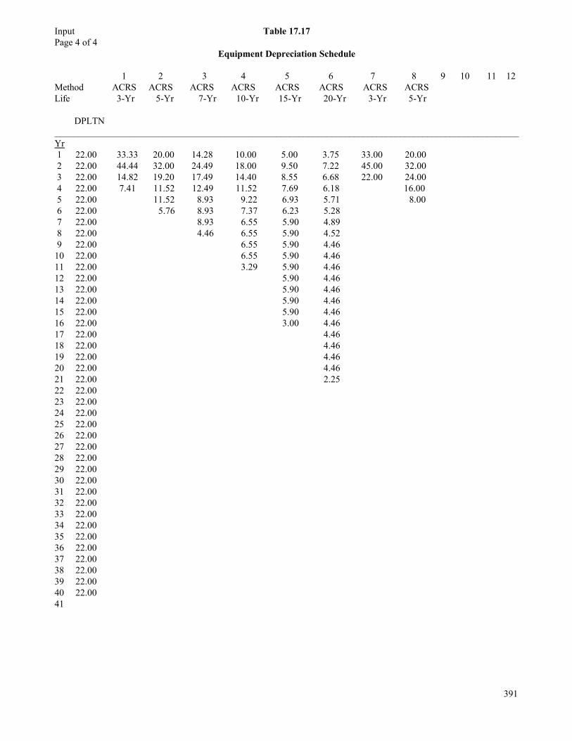
Input Table 17.17Page 4 of 4
Equipment Depreciation Schedule
1 2 3 4 5 6 7 8 9 10 11 12Method ACRS ACRS ACRS ACRS ACRS ACRS ACRS ACRSLife 3-Yr 5-Yr 7-Yr 10-Yr 15-Yr 20-Yr 3-Yr 5-Yr
DPLTN____________________________________________________________________________________________________Yr 1 22.00 33.33 20.00 14.28 10.00 5.00 3.75 33.00 20.00 2 22.00 44.44 32.00 24.49 18.00 9.50 7.22 45.00 32.00 3 22.00 14.82 19.20 17.49 14.40 8.55 6.68 22.00 24.00 4 22.00 7.41 11.52 12.49 11.52 7.69 6.18 16.00 5 22.00 11.52 8.93 9.22 6.93 5.71 8.00 6 22.00 5.76 8.93 7.37 6.23 5.28 7 22.00 8.93 6.55 5.90 4.89 8 22.00 4.46 6.55 5.90 4.52 9 22.00 6.55 5.90 4.4610 22.00 6.55 5.90 4.4611 22.00 3.29 5.90 4.4612 22.00 5.90 4.4613 22.00 5.90 4.4614 22.00 5.90 4.4615 22.00 5.90 4.4616 22.00 3.00 4.4617 22.00 4.4618 22.00 4.4619 22.00 4.4620 22.00 4.4621 22.00 2.2522 22.0023 22.0024 22.0025 22.0026 22.0027 22.0028 22.0029 22.0030 22.0031 22.0032 22.0033 22.0034 22.0035 22.0036 22.0037 22.0038 22.0039 22.0040 22.0041
391

Output Table 17.18Page 1 of 5
LIFE CYCLE COST ANALYSISfor
The Horsefly Heating DistrictKlamath Falls, Oregon
April 28, 1987
Project Cost (Pv) 1,759.954 Benefit Cost Ratio 0.39 to 1Equity Financing (Pv) 295,078 Return on Equity 14.825%Debt Financing (Pv) 2,100,526 Simple Payback 8 years 5 monthsNet Present Value -1,068,686 Discounted Payback 12 years 2 months
1 2 3 4 5Natural Gas Electricity Property Tax O & M Hot Water Present Present & Insurance Present Revenues System System Present System Proposed
System System
YEAR ZERO AMOUNT 50,500 150,000 2,500 15,000 220,000 1988 0 0 0 0 0 1989 0 0 0 0 0 1990 0 0 0 0 0 1991 0 0 0 0 0 1992 67,964 190,532 2,693 18,250 298,599 1993 72,177 202,155 2,734 18,980 317,411 1994 76,652 214,486 2,775 19,739 337,408 1995 82,018 227,570 2,816 20,529 358,665 1996 87,759 241,452 2,858 21,350 381,261 1997 93,902 256,180 2,901 22,204 405,280 1998 100,476 271,807 2,945 23,092 430,813 1999 107,509 288,387 2,989 24,015 457,954 2000 115,250 305,979 3,034 24,976 486,805 2001 123,548 324,644 3,079 25,975 517,474 2002 132,443 344,447 3,126 27,014 550,075 2003 141,979 365,458 3,172 28,095 584,729 2004 152,201 387,751 3,220 29,219 621,567 2005 163,160 411,404 3,268 30,387 660,726 2006 174,907 436,500 3,317 31,603 702,352 2007 187,501 463,126 3,367 32,867 746,600
TOTALS: 1,879,446 4,931,880 48,296 398,293 7,857,719
392
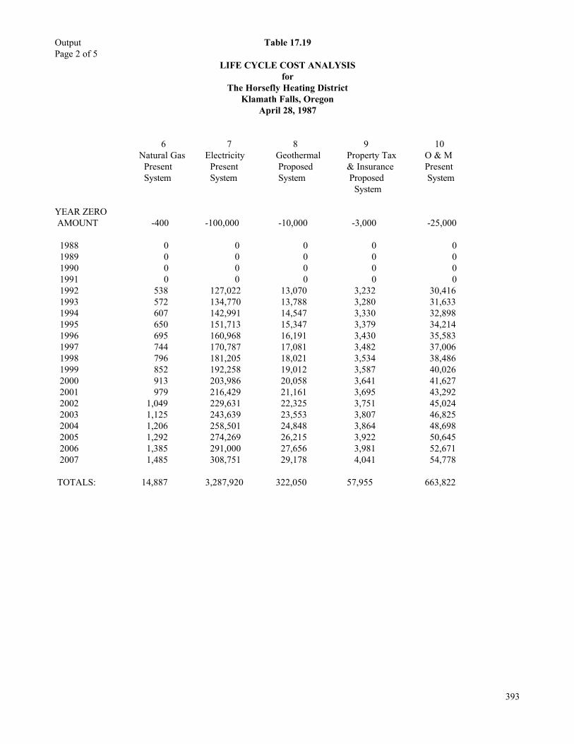
Output Table 17.19Page 2 of 5
LIFE CYCLE COST ANALYSISfor
The Horsefly Heating DistrictKlamath Falls, Oregon
April 28, 1987
6 7 8 9 10Natural Gas Electricity Geothermal Property Tax O & M Present Present Proposed & Insurance Present System System System Proposed System
System
YEAR ZERO AMOUNT -400 -100,000 -10,000 -3,000 -25,000
1988 0 0 0 0 0 1989 0 0 0 0 0 1990 0 0 0 0 0 1991 0 0 0 0 0 1992 538 127,022 13,070 3,232 30,416 1993 572 134,770 13,788 3,280 31,633 1994 607 142,991 14,547 3,330 32,898 1995 650 151,713 15,347 3,379 34,214 1996 695 160,968 16,191 3,430 35,583 1997 744 170,787 17,081 3,482 37,006 1998 796 181,205 18,021 3,534 38,486 1999 852 192,258 19,012 3,587 40,026 2000 913 203,986 20,058 3,641 41,627 2001 979 216,429 21,161 3,695 43,292 2002 1,049 229,631 22,325 3,751 45,024 2003 1,125 243,639 23,553 3,807 46,825 2004 1,206 258,501 24,848 3,864 48,698 2005 1,292 274,269 26,215 3,922 50,645 2006 1,385 291,000 27,656 3,981 52,671 2007 1,485 308,751 29,178 4,041 54,778 TOTALS: 14,887 3,287,920 322,050 57,955 663,822
393

Output Table 17.20Page 3 of 5
LIFE CYCLE COST ANALYSISfor
The Horsefly Heating DistrictKlamath Falls, Oregon
April 28, 1987
11 12 13 14 15 Equipment Equipment Debt Service Interest Net Replacement Depreciation Bank Loan Charges on Operating Proposed Proposed and/or Financing Income System System Bond Issue
YEAR ZERO AMOUNT
1988 0 0 159,247 132,000 -132,000 1989 0 0 159,247 129,548 -129,548 1990 0 0 159,247 126,875 -126,875 1991 0 0 224,345 163,961 -163,961 1992 0 138,544 224,345 158,276 106,346 1993 0 173,015 224,345 152,276 104,346 1994 0 156,664 224,345 145,243 154,780 1995 0 144,215 224,345 137,790 204,289 1996 0 134,727 224,345 129,633 253,454 1997 0 35,301 224,345 120,705 395,362 1998 0 33,252 224,345 110,932 442,907 1999 0 28,558 224,345 100,236 496,326 2000 0 23,875 224,345 88,528 553,416 2001 0 23,875 159,247 75,713 609,576 2002 735,962 179,888 159,247 68,195 507,242 2003 0 171,663 60,000 60,000 572,823 2004 0 167,913 60,000 60,000 628,930 2005 0 164,163 1,060,000 60,000 688,439 2006 0 164,163 0 0 807,822 2007 0 0 0 0 1,035,229
TOTALS: 735,962 1,739,815 4,219,688 2,019,688 7,009,498
394
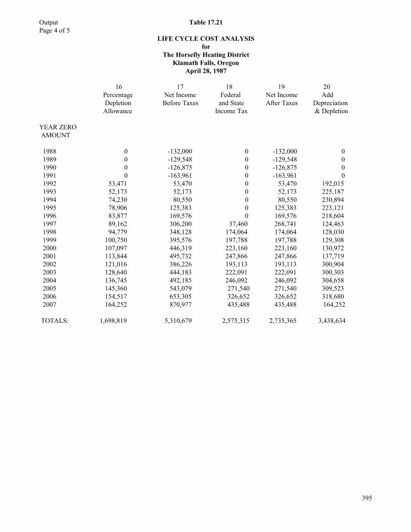
Output Table 17.21Page 4 of 5
LIFE CYCLE COST ANALYSISfor
The Horsefly Heating DistrictKlamath Falls, Oregon
April 28, 1987
16 17 18 19 20 Percentage Net Income Federal Net Income Add Depletion Before Taxes and State After Taxes Depreciation Allowance Income Tax & Depletion
YEAR ZERO AMOUNT
1988 0 -132,000 0 -132,000 0 1989 0 -129,548 0 -129,548 0 1990 0 -126,875 0 -126,875 0 1991 0 -163,961 0 -163,961 0 1992 53,471 53,470 0 53,470 192,015 1993 52,173 52,173 0 52,173 225,187 1994 74,230 80,550 0 80,550 230,894 1995 78,906 125,383 0 125,383 223,121 1996 83,877 169,576 0 169,576 218,604 1997 89,162 306,200 37,460 268,741 124,463 1998 94,779 348,128 174,064 174,064 128,030 1999 100,750 395,576 197,788 197,788 129,308 2000 107,097 446,319 223,160 223,160 130,972 2001 113,844 495,732 247,866 247,866 137,719 2002 121,016 386,226 193,113 193,113 300,904 2003 128,640 444,183 222,091 222,091 300,303 2004 136,745 492,185 246,092 246,092 304,658 2005 145,360 543,079 271,540 271,540 309,523 2006 154,517 653,305 326,652 326,652 318,680 2007 164,252 870,977 435,488 435,488 164,252
TOTALS: 1,698,819 5,310,679 2,575,315 2,735,365 3,438,634
395

Output Table 17.22Page 5 of 5
LIFE CYCLE COST ANALYSISfor
The Horsefly Heating DistrictKlamath Falls, Oregon
April 28, 1987
21 22 23 24 25 Net Cumulative Discounted Cumulative Discounted Operating Cash Flow Cash Flow Discounted Cash Flow Cash Flow Cash Flow at ROR After Taxes
YEAR ZERO AMOUNT
1988 -159,247 -159,247 -144,770 -144,770 -138,687 1989 -159,247 -318,494 -131,609 -276,379 -120,782 1990 -159,247 -477,741 -119,645 -396,024 -105,188 1991 -224,345 -702,087 -153,231 -549,255 -129,056 1992 179,416 -522,671 111,403 -437,852 89,885 1993 205,068 -371,603 115,756 -322,096 89,473 1994 232,342 -85,260 119,228 -202,868 88,285 1995 261,949 175,688 122,201 -80,667 86,684 1996 293,468 470,156 124,459 43,792 84,576 1997 289,563 759,720 111,639 155,431 72,677 1998 188,681 948,401 66,132 221,563 41,243 1999 202,987 1,151,388 64,678 286,241 38,641 2000 218,315 1,369,702 63,238 349,479 36,194 2001 302,051 1,671,753 79,539 429,018 43,611 2002 -332,998 1,338,756 -79,717 349,301 -41,872 2003 522,395 1,861,150 113,688 462,990 57,206 2004 550,750 2,411,900 108,963 571,953 52,525 2005 -418,938 1,992,963 -75,350 496,603 -34,796 2006 645,333 2,638,296 105,517 602,120 46,679 2007 599,740 3,238,036 89,148 691,268 37,781
TOTALS: 3,238,036 691,268 295,078
396

Input Table 17.23Page 1 of 3
LIFE CYCLE COST ANALYSISfor
The Horsefly Heating DistrictKlamath Falls, Oregon
April 28, 1987
Energy forecast used for this report: 1986 Sample Energy Forcast.* This report is for a taxable entity. Dollar values roundedto the nearest: 1
Capital investment data:Year Of Initial Capital Investment...............................(example: 1988)...........: 1988Year Project Will Be In Production.............................(example: 1990)...........: 1992Project Life In Years......................(enter a whole number from 1 to 40)..........: 20Economic Inflation Rate.......................(enter as a whole number e.g. 7)..........: 4%Discount Rate.................................(enter as a whole number 3.g. 12)..............: 10%
Financing:Beginning of Year 1992 1991 1990 1989 1988 Pr Jt Cost ........... 500,000 300,000 700,000 500,000Equity ........... 60,000 ........... ........... 250,000Bank Loan ........... 400,000 ........... ........... 800,000
Life ........... 10 ........... ........... 15(APR) ...........% 10% ...........% ...........% 9%
Bond Issue ........... ........... ........... ........... 1,000,000Life ........... ........... ........... ........... 18(APR) ...........% ...........% ...........% ...........% 6%
Invested ........... 1,157 241,366 642,765 1,390,752(APR) ...........% 8.5% 10% 9% 8%
Investment EOY 1992: 1,255 Total Project Cost (NPV): 1,759,954
Year Zero Annual Costs: Present System Proposed SystemConventional Energy:
Natural Gas........................................................................................ 50,500 400Fuel Oil.............................................................................................. ........... ...........Propane.............................................................................................. ........... ...........Coal.................................................................................................... ........... ...........Electricity........................................................................................... 150,000 100,000
Other Energy:Geothermal....................................................................................... ........... 10,000Solar................................................................................................. ........... ...........Nuclear............................................................................................ ........... ...........Biomass........................................................................................... ........... ...........Waste Heat...................................................................................... ........... ...........
Insurance............................................................................................... 2,500 3,000Inflation Rate................................................................................... 1.5%
Operation and Maintenance.................................................................. 15,000 25,000Inflation Rate................................................................................... 4%
397
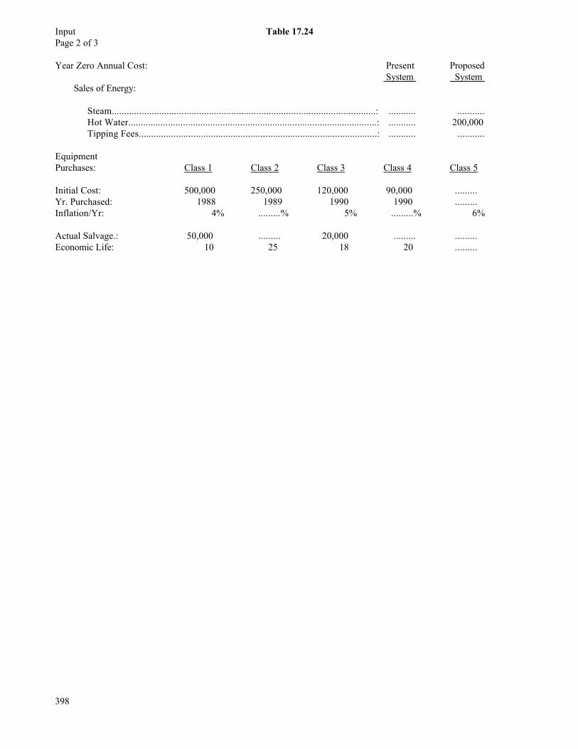
Input Table 17.24Page 2 of 3
Year Zero Annual Cost: Present Proposed System System
Sales of Energy:
Steam..........................................................................................................: ........... ...........Hot Water....................................................................................................: ........... 200,000Tipping Fees................................................................................................: ........... ...........
EquipmentPurchases: Class 1 Class 2 Class 3 Class 4 Class 5
Initial Cost: 500,000 250,000 120,000 90,000 .........Yr. Purchased: 1988 1989 1990 1990 .........Inflation/Yr: 4% .........% 5% .........% 6%
Actual Salvage.: 50,000 ......... 20,000 ......... .........Economic Life: 10 25 18 20 .........
398

Input Table 17.25Page 3 of 3
Sample Energy Forecast*Forecast Energy Inflation Rates
1986
1 2 3 4 5 6 7 8 9 10 11 12 13Natu Fuel Prop Coal Elec Geot Sola Nucl Biom Wast Stea Hot Tipp
(1) (2) (3) (4) (5) (1) (2) (3)_______________________________________________________________________________________________________________________________________Yr86 0.020 0.019 0.019 0.020 0.009 0.015 0.004 0.001 0.005 0.010 0.002 0.023 0.02387 0.020 0.019 0.019 0.020 0.009 0.015 0.004 0.001 0.005 0.010 0.002 0.023 0.02388 0.020 0.019 0.019 0.020 0.009 0.015 0.004 0.001 0.005 0.010 0.002 0.023 0.02389 0.020 0.019 0.019 0.020 0.009 0.015 0.004 0.001 0.005 0.010 0.002 0.023 0.02390 0.022 0.019 0.019 0.020 0.009 0.015 0.004 0.001 0.005 0.010 0.002 0.023 0.02391 0.022 0.019 0.019 0.020 0.009 0.015 0.004 0.001 0.005 0.010 0.002 0.023 0.02392 0.022 0.019 0.019 0.020 0.009 0.015 0.004 0.001 0.005 0.010 0.002 0.023 0.02393 0.022 0.019 0.019 0.020 0.021 0.015 0.004 0.001 0.005 0.010 0.002 0.023 0.02394 0.022 0.019 0.019 0.020 0.021 0.015 0.004 0.001 0.005 0.010 0.002 0.023 0.02395 0.030 0.019 0.019 0.020 0.021 0.015 0.004 0.001 0.005 0.010 0.002 0.023 0.02396 0.030 0.019 0.019 0.020 0.021 0.015 0.004 0.001 0.005 0.010 0.002 0.023 0.02397 0.030 0.019 0.019 0.020 0.021 0.015 0.004 0.001 0.005 0.010 0.002 0.023 0.02398 0.030 0.019 0.019 0.020 0.021 0.015 0.004 0.001 0.005 0.010 0.002 0.023 0.02399 0.030 0.019 0.019 0.020 0.021 0.015 0.004 0.001 0.005 0.010 0.002 0.023 0.02300 0.032 0.018 0.018 0.020 0.021 0.015 0.004 0.001 0.005 0.010 0.002 0.023 0.02301 0.032 0.018 0.018 0.020 0.021 0.015 0.004 0.001 0.005 0.010 0.002 0.023 0.02302 0.032 0.018 0.018 0.020 0.021 0.015 0.004 0.001 0.005 0.010 0.002 0.023 0.02303 0.032 0.018 0.018 0.020 0.021 0.015 0.004 0.001 0.005 0.010 0.002 0.023 0.02304 0.032 0.018 0.018 0.020 0.021 0.015 0.004 0.001 0.005 0.010 0.002 0.023 0.02305 0.032 0.018 0.018 0.020 0.021 0.015 0.004 0.001 0.005 0.010 0.002 0.023 0.023

Output Table 17.26Page 1 of 4
LIFE CYCLE COST ANALYSISfor
The Horsefly Heating DistrictKlamath Falls, Oregon
April 28, 1987
Project Cost (Pv) 1,759.954 Benefit Cost Ratio 0.72 to 1Equity Financing (Pv) 295,078 Return on Equity 18.737%Debt Financing (Pv) 2,100,526 Simple Payback 8 years 5 monthsNet Present Value -500,433 Discounted Payback 11 years 0 monthsDiscount Rate 10.00%
1 2 3 4 5Natural Gas Electricity Insurance O & M Hot Water Present Present Present Present Revenues System System System System Proposed
System
YEAR ZERO AMOUNT 50,500 150,000 2,500 15,000 220,000
1988 0 0 0 0 0 1989 0 0 0 0 0 1990 0 0 0 0 0 1991 0 0 0 0 0 1992 67,964 190,532 2,693 18,250 298,599 1993 72,177 202,155 2,734 18,980 317,411 1994 76,652 214,486 2,775 19,739 337,408 1995 82,018 227,570 2,816 20,529 358,665 1996 87,759 241,452 2,858 21,350 381,261 1997 93,902 256,180 2,901 22,204 405,280 1998 100,476 271,807 2,945 23,092 430,813 1999 107,509 288,387 2,989 24,015 457,954 2000 115,250 305,979 3,034 24,976 486,805 2001 123,548 324,644 3,079 25,975 517,474 2002 132,443 344,447 3,126 27,014 550,075 2003 141,979 365,458 3,172 28,095 584,729 2004 152,201 387,751 3,220 29,219 621,567 2005 163,160 411,404 3,268 30,387 660,726 2006 174,907 436,500 3,317 31,603 702,352 2007 187,501 463,126 3,367 32,867 746,600
TOTALS: 1,879,446 4,931,880 48,296 398,293 7,857,719
400

Output Table 17.27Page 2 of 4
LIFE CYCLE COST ANALYSISfor
The Horsefly Heating DistrictKlamath Falls, Oregon
April 28, 1987
6 7 8 9 10Natural Gas Electricity Geothermal Insurance O & M Present Present Proposed Proposed Operating
System System System System Cash Flow
YEAR ZERO AMOUNT -400 -100,000 -10,000 -3,000 -25,000
1988 0 0 0 0 0 1989 0 0 0 0 0 1990 0 0 0 0 0 1991 0 0 0 0 0 1992 538 127,022 13,070 3,232 30,416 1993 572 134,770 13,788 3,280 31,633 1994 607 142,991 14,547 3,330 32,898 1995 650 151,713 15,347 3,379 34,214 1996 695 160,968 16,191 3,430 35,583 1997 744 170,787 17,081 3,482 37,006 1998 796 181,205 18,021 3,534 38,486 1999 852 192,258 19,012 3,587 40,026 2000 913 203,986 20,058 3,641 41,627 2001 979 216,429 21,161 3,695 43,292 2002 1,049 229,631 22,325 3,751 45,024 2003 1,125 243,639 23,553 3,807 46,825 2004 1,206 258,501 24,848 3,864 48,698 2005 1,292 274,269 26,215 3,922 50,645 2006 1,385 291,000 27,656 3,981 52,671 2007 1,485 308,751 29,178 4,041 54,778
TOTALS: 14,887 3,287,920 322,050 57,955 663,822
401

Output Table 17.28Page 3 of 4
LIFE CYCLE COST ANALYSISfor
The Horsefly Heating DistrictKlamath Falls, Oregon
April 28, 1987
11 12 13 14 Equipment Debt Service Net Cumulative Replacement Bank Loan Operating Cash Flow Proposed and/or Cash Flow System Bond Issue
YEAR ZERO AMOUNT
1988 0 159,247 -159,247 -159,247 1989 0 159,247 -159,247 -318,494 1990 0 159,247 -159,247 -477,741 1991 0 224,345 -224,345 -702,087 1992 0 224,345 179,416 -522,671 1993 0 224,345 205,068 -317,603 1994 0 224,345 232,342 -85,260 1995 0 224,345 261,949 176,688 1996 0 224,345 293,468 470,156 1997 0 224,345 327,023 797,179 1998 0 224,345 362,745 1,159,924 1999 0 224,345 400,775 1,560,699 2000 0 224,345 441,474 2,002,174 2001 0 159,247 549,917 2,552,091 2002 735,962 159,247 -183,177 2,368,914 2003 0 60,000 744,486 3,113,400 2004 0 60,000 796,843 3,910,243 2005 0 1,060,000 -147,398 3,762,844 2006 0 0 971,985 4,734,830 2007 0 0 1,035,229 5,770,058
TOTALS: 735,962 4,219,688 5,770,058
402

Output Table 17.29Page 4 of 4
LIFE CYCLE COST ANALYSISfor
The Horsefly Heating DistrictKlamath Falls, Oregon
April 28, 1987
15 16 17 Discounted Cumulative Discounted Cash Flow Discounted Cash Flow Cash Flow at ROR
YEAR ZERO AMOUNT
1988 -144,770 -144,770 -134,118 1989 -131,609 -276,379 -112,954 1990 -119,645 -396,024 -95,130 1991 -153,231 -549,255 -112,870 1992 111,403 -437,852 76,022 1993 115,756 -322,096 73,180 1994 119,228 -202,868 69,829 1995 122,201 -80,667 66,304 1996 124,459 43,792 62,561 1997 126,081 169,874 58,713 1998 127,140 297,014 54,850 1999 127,699 424,713 51,037 2000 127,879 552,592 47,349 2001 144,810 697,403 49,673 2002 -43,851 653,552 -13,935 2003 162,022 815,574 47,699 2004 157,651 973,225 42,997 2005 -26,511 946,714 -6,698 2006 158,927 1,105,641 37,201 2007 153,880 1,259,521 33,369
TOTALS: 1,259,521 295,078
403

GLOSSARY OF ENGINEERING COST ANALYSISTERMS
Accelerated cost recovery system (ACRS) - Adepreciation system developed in 1987 which provides morerapid cost recovery than straight line depreciation.
Annual effective interest rate - The actual or true annualinterest rate that indicates the exact amount of interest paidper year by converting nominal or annual percentage ratesto the actual dollar amount of interest annually.
Annual equivalent cost - The amount of an equal end-of-year payment series that is equivalent to present or futurevalue when the interest rate is considered.
Annual percentage rate (APR) - The interest rate per yearwithout considering the effect of compounding followed bythe number of compounding periods per year.
Annuity due - An equal series of beginning-of-the-periodpayments.
Arithmetic gradient - An end-of-period payment series thatincreases each period by a constant amount.
Asset Depreciation Range (ADR) - The life of an asset asfixed by the Internal Revenue Code.
Benefit-cost ratio - The ratio that results in dividing thepresent value of all benefits of a project by the present valueof all the costs of that same project.
Book value - The cost basis of an asset less the accumulateddepreciation.
Business tax credit - A direct credit to the tax liability of afirm because of the purchase or operation of assets that areeligible for business tax credits under the current tax law.
Capital recovery - The process of charging periodic end-of-period payment series that is equivalent to the initial assetcost less the expected salvage value at the end of itseconomic life.
Capital recovery factor - The factor used to calculate theend-of-period payment series that is equivalent to the cost ofan asset less its future salvage value based on thecompounded interest rate.
Cash flow - 1. The actual flow of dollars into and out of theoperation of a capital venture. 2. The flow of revenues lessoperating costs plus depreciation from a given capitalventure.
404
Compound amount factor - 1. The future value of a lumpsum considering time and the compound interest rate. 2.The future value of a payment series considering time andthe compound interest rate.
Compound interest - Interest that is calculated and addedto the initial amount such that future interest earnings willbe accumulated based on the total amount including interest.
Cost of capital - The costs incurred because of borrowingmoney. Normally expressed as an interest rate.
Depletion - A method of depreciation applying to depletableresources such as geothermal, coal, timber, oil, and naturalgas.
Depreciation - A method of expensing the decrease in valueof an asset over its life span and charging these costs tooperations.
Discounted cash flow - Evaluating the annual costs andrevenues associated with a venture over the years of its lifeat some interest rate to arrive at a present value of these cashflows.
Discounted payback period - The time period required(considering the time value of money) for the revenues orbenefits of a project equal the capital investment andoperating costs of that project.
Discount rate - The interest rate used to evaluate the cashflows resulting from the operation of a project.
Double declining balance depreciation - A method ofaccelerated depreciation that applies twice the straight linerate multiplied by the book value of the asset.
Economic life - The period of time from installation toretirement of an asset that minimizes the cost of buying,installing, operating and salvaging that asset.
Energy tax credit - A direct credit to the tax liability of afirm because of the purchase or operation of assets that areeligible for energy tax credits under the current tax law.
Equipment cost basis - The adjusted cost of an asset due toadditional installation costs or subtracted tax credits claimedwhich alter the amount of depreciation which may beclaimed.
Equipment replacement life - The period of time that willelapse from initial installation until a piece of equipment iseither obsolete or worn out and requires replacement.

Future value/future work - The equivalent value at adesignated future date of previous cash flows evaluated overtime at a compound interest rate.
Geometric gradient - An end-of-period payment series thatincreases each period by the exact same percentage.
Inflation - An increase in prices in general usually causedby a decline in the purchasing power of a monetary system.
Interest - The periodic cost charged for borrowing money.
Internal rate of return - The interest rate earned byinvesting in a particular venture and receiving cash flows asa result of that investment without regard to any otherinvestments.
Investment tax credit - A direct credit to the tax liability ofa firm because of the purchase of assets that are eligible forinvestment tax credits under the current tax law.
Modified Accelerated Cost Recovery System (MACRS) -The current method of depreciation in which property classlife and decpreciation methods are set by law, and salvagevalue is treated as zero.
Marginal cost - The amount of cost associated with anincrease in output or with a particular project.
Marginal tax rate - The amount of taxes (expressed as a %)because of an increase in output or the income of aparticular project.
Net present value - The equivalent value at time zero(today) of the net difference between future cost and revenuecash flows evaluated (discounted) over time at a compoundinterest rate.
Nominal interest rate - The interest rate per year withoutconsidering the effect of compounding followed by thenumber of compounding periods per year.
Ordinary annuity - A stream of equal end-of-periodpayments.
Opportunity cost - The cost of not taking advantage of aninvestment opportunity because of limited capital, resources,or other conflicting circumstances and thereby losing theearnings or benefits associated with that investment.
Present value/present worth - The equivalent value at timezero (today) of future cash flows evaluated (discounted) overtime at a compound interest rate.
Rate of return (ROR) - The compound interest rate thatwill cause the present value of all the costs and benefitsassociated with a project to equal exactly zero.
Salvage value - 1. The value obtained from an asset whensold, scrapped or retired from service. 2. The current fairmarket value of a piece of equipment.
Sensitivity - The amount of effect or impact experienced bychanging one of the input variables of a project undergoingan engineering economic study in order to alter theacceptability or rejectability of that project.
Simple interest - Interest that is accrued periodically ononly the original amount of a loan or investment, and that isnot compounded.
Simple payback period - The time period required (withoutconsidering the time value of money) for the revenues orbenefits of a project to equal the capital investment andoperating costs of that project.
Sinking fund - A stream of equal end-of-period paymentsset aside in an investment fund for the purpose of replacingan asset or making a balloon payment on a debt.
Straight line depreciation - A method of depreciation inwhich the equipment cost basis of an asset is recovered inequal amounts over its taxable life based on time, units ofoutput, miles driven, or hours of operation.
Sum-of-the-years-digits depreciation (SYD) - A methodof accelerated depreciation in which the equipment costbasis of an asset is multiplied each year by the remainingyears of life divided by [(n times n+1) divided by 2] to arriveat a depreciation charge for that year (where n equals thetaxable life of the asset).
Sunk cost - A capital cost already incurred that cannot berecovered and is not to be considered or evaluated in makingcurrent decisions.
Time value of money - The future, present or annualequivalent value of cash flows considering the compoundinterest rate of borrowed money, the expected rate ofearnings on invested capital, or the required rate of returnon the capital investment required for a project.
REFERENCES
Anderson, D. N. and J. W. Lund, editors, 1979. Geothermal Resources Council Special Report No. 7:Direct Utilization of Geothermal Energy - A TechnicalHandbook, U.S. Department of Energy, Washington,DC.
Lienau, P. J., et al., 1978. Agribusiness GeothermalEnergy Utilization Potential of Klamath and WesternSnake River Basins, Oregon, U.S. Department ofEnergy, Washington, DC.
405

Newnan, D. G., 1988. Engineering Economic Analysis,3rd edition, Engineering Press Inc., San Jose, CA.
Riggs, J. L. and T. M. West, 1986. EngineeringEconomics, 3rd edition, McGraw-Hill Book Co.,NY.
Thuesen, G. H. and W. J. Fabrycky, 1984. EngineeringEconomy, 6th edition, Prentice-Hall Inc., EnglewoodCliffs, NJ.
406


![[PPT]Cost and Supply of Geothermal Power - Utahfiles.geology.utah.gov/emp/geothermal/ugwg/workshop0805/... · Web viewTitle Cost and Supply of Geothermal Power Author Susan Petty](https://static.fdocuments.in/doc/165x107/5ae9830b7f8b9ad73f8bed71/pptcost-and-supply-of-geothermal-power-viewtitle-cost-and-supply-of-geothermal.jpg)


