Energy Reduction and Sustainability ThroughTotal Energy Management (TEM) Program

PSCI 2011Monterey, CA

2

• Founded in 1950, Husky is world’s largest Injection Molding equipment supplier

• A technology and environmental leader with history of innovation

• 3300 employees worldwide

• Bought by Onex, a leading North American private equity firm, in 2006

Husky Injection Molding Systems

3

Manufacturing Advisory Services

Provide operational consulting, design and project management services to support our existing and prospective customers

1. Consulting and Advisory Services• Comprehensive plant & operational assessment• Operational performance improvement & implementation• Facility planning and optimization • Total Energy Management Program

2. Building and Infrastructure Planning and Design3. Project Management and Turnkey services

4

Two Approaches to Reduce Energy Cost

1. Reduce the cost per unit of energy ($/KWh) through negotiation and risk mitigation

• Numerous consulting firms provide “Negotiation and risk mitigation” services

• Alternative Energy generation

2. Reduce the amount of energy used (KW/lb): • Certain utility companies offer programs that provide molders

rebates towards the purchase and installation of qualified equipment that improves their facility’s energy efficiency

These two approaches alone without an “Energy Management Program” can not be sustainable

5

• Phase 1: Plant energy audits

• Phase 2: Implementation of policies and procedures to measure, set targets, and monitor energy related KPIs to continuously reduce and sustain energy consumption

Total Energy Management

6

• A total of $2.7M saved since 2000– 30% reduction in KWh consumption

(17,000,000 KWh or 1,800 metric tons of CO2)

TEM Case Study - Husky

40,000,000

45,000,000

50,000,000

55,000,000

60,000,000

65,000,000

70,000,000

2000 2001 2002 2003 2004 2005 2006 2007 2008

Years

KWh

Do Nothing

Actual

17,000,000 KWhOR 30%reduction

7

Common Energy KPIs

X

0

20000

40000

60000

80000

100000

120000

140000

160000

1 2 3 4 5 6 7 8 9 10 11 12 13 14 15 16 17 18 19 20

Weeks

KW

h/ w

eek

0

20

40

60

80

100

120

140

160

180

Prod

uctio

n (T

onne

s/ w

eek)

Energy (KWh / week)Production (Tonnes/ week)

0

200

400

600

800

1000

1200

1400

1 2 3 4 5 6 7 8 9 10 11 12 13 14 15 16 17 18 19 20

Weeks

KWh/

tonn

e

KWh/ Tonne

Although KWh/ Lb is a widely acceptable energy KPI, it fails to show if the energy consumption is optimized

8

1 - Understand your “Base” and “Process” loads

2 - Create site energy profile3 - Understand when and how much energy is used 4 - Identify, Quantify, and Prioritize opportunities 5 - Eliminate waste and reduce consumption through

- Implementation of selected energy reduction projects6 - Monitoring and Targeting

- Understand Where energy is used7 - Data analysis and reporting energy KPIs

- (Energy dashboard) by department8 - Conduct internal and external benchmarking9 - Repeat the steps – Continuous improvement

Total Energy Management Program

Phase 1:Energy audit& reductionstrategy

Phase 2:SustainabilityThroughM&T

9

-

100,000

200,000

300,000

400,000

500,000

600,000

700,000

800,000

- 50,000 100,000 150,000 200,000 250,000 300,000 350,000 400,000

Production volume (Kg or Lb)

Ene

rgy

usag

e (K

Wh)

• Energy has variable and fixed costs and both can be affected• Performance Characteristic Line (PCL) provides an operational signature

of the plant that is closely related to the way the plant management runs the plant

1 - Identify Base & Process Loads

10Preliminary Analysis – Case Study

• Overall plant process load (1.16 KWh/Kg) is within ballpark. • Overall plant base load (15,706 Kwh/ day) is approx. 51% of the total average

load. This seems to be very high and typically an indication of electrical usage in the plant which may not be related to production. (low hanging fruit)

• Correlation coefficient (R2) which indicates linearity between energy usage and production volume is very low (0.454). This typically indicates poor control of electrical usage.

Linear Regression Analysis Tool7 Electricity Production

Month Date kWh Kg/day Include1 1-Jan-09 29,230 14,473 Yes2 1-Feb-09 23,585 9,434 Yes3 1-Mar-09 34,991 16,931 Yes4 1-Apr-09 32,629 14,632 Yes5 1-May-09 33,531 14,552 Yes6 1-Jun-09 30,726 12,602 Yes7 1-Jul-09 35,097 12,557 Yes8 1-Aug-09 33,864 12,355 Yes9 1-Sep-09 29,852 11,810 Yes10 1-Oct-09 32,869 13,684 Yes11 1-Nov-09 30,070 12,130 Yes12 1-Dec-09 27,722 11,551 Yes13 1-Jan-10 30,052 14,310 Yes

Regression ModelMonths 13 Dependent Variable . . . Electricity

Cooling Balance Point Temp 18 Independent Variable . ProductionSlope. . . . . . . . . . . . . . 1.169 kWh/Kg

Heating Balance Point Temp 18 Date Intercept. . . . . . . . . . . . 15,706 kWh/dayor R2 . . . . . . . . . . . . . . . . . 0.454

Sequence #

1-Jan-09

Edit Historical Data

1

0

5,000

10,000

15,000

20,000

25,000

30,000

35,000

40,000

0 2000 4000 6000 8000 10000 12000 14000 16000 18000

Production (Kg/day)

Elec

tric

ity (k

Wh)

Production

X-Y Graph

Line Graph

Ex/Include Point

Independent Variable is:

Duration

Starting

Degree Day Parameters

11

2- Site Energy Profile

• Create Site energy profile through actual on-site measurements

Measured consumption break down

Film Extruder4.5%Thermoformer

2.5%

Process Water system16.5%

Handle Machines1.3%

Wrapping Machines0.0%

Compressed air 8.7%

Printers4.4%

Feed Systems1.6%

Cranes0.1%

Injection Molding Machine51.5%

Plant Lighting8.9%

12

3 – Understand “When” and “How much”

Peak at 1,700KW

Base load at 300KW (25% of average load)Goal is to be @ 10% of average load

Average PF of 0.84Goal is to be above 0.9

0 10 20 30 40 50 60 70 80 90 100Percent of Time for Load Duration

Chronological Time for Demand Profile

Only 5% of time over 1,600 KW

13

1 - Ud nderstanyour “Base” and “Process” loads

2 - Create site energy profile3 - Understand when and how much energy is used4 - Identify, Quantify, and Prioritize opportunities 5 - Eliminate waste and reduce consumption through

- Implementation of selected energy reduction projects6 - Monitoring and Targeting

- Understand Where energy is used7 - Data analysis and reporting energy KPIs

- (Energy dashboard) by department8 - Conduct internal and external benchmarking9 - Repeat the steps – Continuous improvement

Total Energy Management Program

Phase 1:Energy audit& reductionstrategy

Phase 2:SustainabilityThroughM&T

14

Typical Part Cost and Energy Break Down

ENERGYENERGY

Resin86%

Labour2%Energy

3%

Equipment5%

Infrastructure2%

Maintenance2%

Machines50%

Lighting3%

d cooling12%

Dryers20%

HVAC8%

Air compressors6% Others

1%

15

Machines50%

Others1%

Air compressors6%HVAC

8%

Dryers20%

Mold cooling12%

Lighting3%Machine Cooling

Cooling Towers

• Contamination in water• Scale and oxidation in

pipes• High water and chemical

consumption• Cost of water disposal

Dry Coolers

• Clean water to process• No scale or corrosion• Minimal maintenance• Reduced energy

consumption• No water disposal• No water treatment

chemical consumption

16

Adiabatic Dry Coolers

• Ambient air (dry bulb) is used to cool the water• Clean water to process• No scale or corrosion, minimal maintenance• Reduced energy consumption• No water disposal• No water treatment chemical consumption • Adiabatic cooling – maintains ability to deliver

cool water even in HOT ambient conditions with minimal water consumption

• DC Variable Speed fans – extremely low energy consumption

• Less than 20 times less water than tower

17Energy Saving by Heat Recovery

Tank38°C

Tank34°C

Dryer DryerHydraulicHydraulic

Dry CoolerPumps

ConsumerPumps

Refrigerant Circuit

Heat Exchanger

M

Air Heater

M

Air Heater

38°C

50°C

34°C

40°C

Room size: 6m x 30m x 50mRoom volume: ~ 9.000m³Outside temperature: -10°CRoom temperature: 18°C

HyPET300 E120(800kg/h)

18Mold Cooling

0.00

5.00

10.00

15.00

20.00

1 2 3 4 5 6 7 8 9 10 11 12

Leaving chilled water temperature

% in

crea

se in

Chi

llers

' CO

P

Absorption

Reciprocating

Centrifugal

Screw

(C)

1- Water Temperature:• Typically every 1oF increase in leaving water temperature results

to 2% to 3% reduction in energy consumption

2- Technology

19Free Cooling

20Free Cooling

Effect of 43F vs. 50F chilled water temp. on free cooling:

• 15% of the year with 50oF (including dry cooler and heat exchanger approach)

• 4% of the year with 43oF (including dry cooler and heat exchanger approach)

• Estimated savings around € 40,000/ year Vs. € 11,000/ year

Temperature vs. Time - Middlesex UK

0

5

10

15

20

25

11/14/2007 1/3/2008 2/22/2008 4/12/2008 6/1/2008 7/21/2008 9/9/2008 10/29/2008 12/18/2008 2/6/2009

Date

Tem

pera

ture

(deg

C)

15% of the year is colder than 4.5°C, compared to 4.26% of the year colder than 0.5°C

21

Machines50%

Lighting3%

Mold cooling12%

Dryers20%

HVAC8%

Air compressors6%

Others1%

Compressed Air

• Compressors are only 5-15% efficient

• Compressed air is expensive energy– At point of use compressed air costs 10

times more than equivalent quantity of electrical power

• Most of the life cycle cost of a compressor is in the energy it uses

Energy cost, 75%

Capital cost, 15%

Maintenance, 10%

22

Operating Conditions Influence Energy Costs

• Part load operation– 40–80% of full kW at part load

• System pressure – each 5psi = up to 5% more power

• Air inlet temperature– each 7oF lower = 1% more air

• Pipe sizing – Each 5psi drop = 2% more energy

• Leaks commonly constitute 25% of total compressed air use

Size CFM HP $/Yr

1/4” 104 26 $15,300

One 1/4" leak is equal to 300 60-watt lamps!

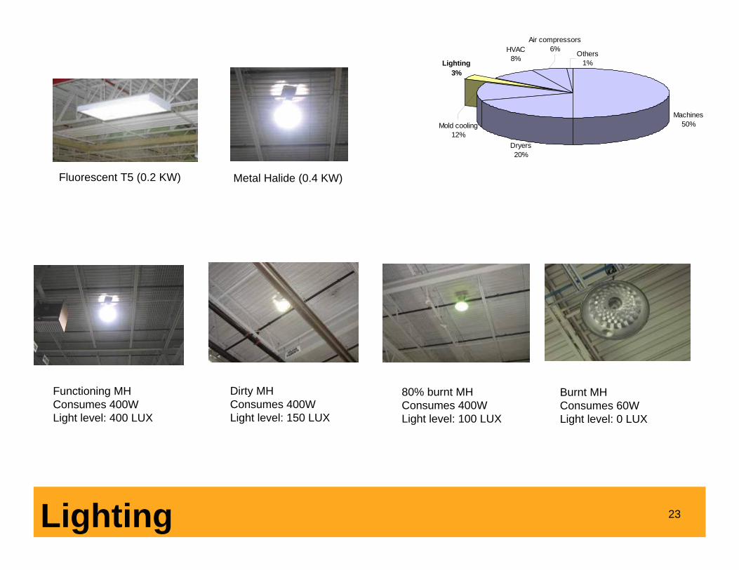
23Lighting

Machines50%

Others1%

Air compressors6%HVAC

8%

Dryers20%

Mold cooling12%

Lighting3%

Fluorescent T5 (0.2 KW)

Functioning MH Consumes 400WLight level: 400 LUX

80% burnt MH Consumes 400WLight level: 100 LUX

Dirty MH Consumes 400WLight level: 150 LUX

Burnt MH Consumes 60WLight level: 0 LUX

Metal Halide (0.4 KW)

24Effect of Cycle Time on Energy

Base Line Exit

Temperature

Faster Cycle

Exit Temperature

Equipment Description Measured Power (kW)

Power Factor 480V

Cycle Time (sec)

Part Weight

(g)

Number of Parts per

Cycle

Machine Process Load

(kW/kgHr)

Before Husky-HL160RS55/50 30.440 0.76 13.4 174 1 0.651

After Husky-HL160RS55/50 30.811 0.76 12.6 174 1 0.613

Percent improvement 6% 6%

Machines50%

Lighting3%

Others1%

Air Compressors6%

Dryers20%

Cooling12%

HVAC8%

25Effect of Throughput on Energy

0.0

0.5

1.0

1.5

2.0

2.5

H101 H102 H103 H104 H105 H106 H107 H108 H109 H110 H113 H114 H115 H116 H117 H118 H119

Mac

hine

ene

rgy

Cons

umpt

ion

(Kw

h/ K

g)

0%

20%

40%

60%

80%

100%

120%

140%

160%

180%

200%KWh/ Kg (Standard Throughput)KWh/ Kg (Actual Throughput)Percentage Difference

• Reduction in throughput due to cavity/ cycle deviation increases the KWh/ Lb of processed resin

26

Other Energy Reduction Opportunities

Power Factor:

“Over $16 billion dollars of Electricity is unusable energy, but billable in the U.S."U.S. Dept. Of Energy

27

Operations• Operational efficiencies have major impact on energy consumption

(OEE)– Unscheduled down time, Scrap, Cycle and Cavitations efficiency– Excessive mold change time will waste energy if the machine is idling. QMC saves energy and

increases OFE

• Staggering start-ups preferably at off peak rates (reduces demand charges)

• Turn the machine’s motor on after the machine heat is closed to the set temperature (Improves PF)

• Size equipment right – Lightly loaded machines tend to have low Power Factor– Motors are more efficient near design loads

• Switch machines and/or dryers off for idle periods longer than 20 min• Stop circulating water through mold when idle• Use barrel insulation if possible (Generally under one year payback)• Chilled water at the highest temperature without affecting cycle time

28

Electric Motors

• Electrical motors account for 40% to 60% of the electricity used in a typical molding plant

• Considering the “Life Cycle Costing”, the cost of energy to run a motor is generally 150 times the cost of purchasing that motor

• Match the motor to the load. Motors are more efficient near the design load– Motors are most efficient running at 80% to 90% of their rated loads– Large motors at part load are less efficient than small motors at full

load – A lightly loaded motor could reduce PF

• Rewinding motors builds in 1% permanent inefficiency in the motor

29

1 - Estimate and verify site energy profile2 - Understand your “Base” and “Process” loads3 - Understand when and how much energy is used 4 - Identify, Quantify, and Prioritize opportunities 5 - Eliminate waste and reduce consumption through

- Implementation of selected energy reduction projects6 - Monitoring and Targeting

- Understand Where energy is used7 - Data analysis and reporting energy KPIs

- (Energy dashboard) by department8 - Conduct internal and external benchmarking

Total Energy Management Program

Phase 1:Energy audit& reductionstrategy

Phase 2:SustainabilityThroughM&T

30

6- Monitoring & Targeting

• Energy is a controllable cost that should be monitored and controlled in the same way as other direct, production-related costs such as labor, raw materials, parts, and supplies.

• Divide the plant into energy-accountable centers (EAC). – Molding workcell (includes machines and automation)– Auxiliaries (includes chillers, compressors )

• Supervisors and managers of each area are responsible and accountable for energy use – Implement KPI– Set targets– Evaluate

31

• Departments to be accountable for their energy usage by assigning existing meters to each department (to be investigated)

Live Monitoring – Case Study

Current Proposed

Meter 506 Meter 503 Meter 502 Meter 506 Meter 503 Meter 502(2000 Amp) (1000 Amp) (1500 Amp) ? (2000 Amp) (1000 Amp) (1500 Amp) ?

H101 H115 Two Chillers H101 ECKEL 1 Two ChillersH102 H116 Pumps H102 ECKEL 2 One Chiller H103 ECKEL 1 H103 ECKEL 3 PumpsH104 ECKEL 2 H104 ECKEL 5H 105 ECKEL 5 H 105 ECKEL 6H106 One Chiller H106 CST1H 107 H 107 CST2H 108 H 108H 109 H 109H 110 H 110H 113 H 113H114 H114H117 H117H118 H118H119 H119CST1 H115CST2 H116

ECKEL 3 LightingECKEL 6 Sorting machineLighting Conveyors

Sorting machine Bag sealerConveyors DehumidifiersBag sealer Cranes

Dehumidifiers Offices/ Maint.Cranes Air Handlers

Offices/ Maint.Air Handlers

32

0.82

0.83

0.84

0.85

KW

h co

nsum

ptio

n

Type of Energy

Actual Consumption

Design Consumption Actual Value ($) Design Value ($) Profit/ Loss ($)

Electricity 195,345 156,745 11,720 9,407 -2,313

Increase in electrical consumption could be used as a predictive tool to prevent failure

Live Monitoring and Predictive Maintenance

33

Correlation of live process water monitoring and machine parameters reduces reject rates and eliminates process variations

Process Water Flow

Backpressure

Injection Cushion

50

0G

PM

300

0

psi

60

0

g

Live Monitoring and Six Sigma

34Energy on Management Agenda

y = 81.769x + 61366R2 = 0.9961

0

20

40

60

80

100

120

140

160

180

0 200 400 600 800 1,000 1,200 1,400

Thou

sand

s

Production (tonnes)

Ene

rgy

(kW

h)

0

20,000

40,000

60,000

80,000

100,000

120,000

140,000

160,000

180,000

1 2 3 4 5 6 7 8 9 10 11 12

KW

h

Actual KWhForecasted KWh

-40,000

-30,000

-20,000

-10,000

0

10,000

20,000

30,000

40,000

1 2 3 4 5 6 7 8 9 10 11 12 13 14 15 16 17 18 19 20 21 22 23 24

Month

Dev

iatio

n fr

om p

redi

cted

(KW

h)

7 – Data Analysis and Energy KPIs

-100000

-50000

0

50000

100000

150000

200000

250000

300000

350000

400000

1 2 3 4 5 6 7 8 9 10 11 12 13 14 15 16 17 18 19 20 21 22

Month

CU

SUM

(KW

h)

Target CUSUMOriginal CUSUM

35

-700,000

-600,000

-500,000

-400,000

-300,000

-200,000

-100,000

-1 3 5 7 9 11

Month

Elec

tric

ity (k

Wh)

Data Analysis - CUSUM Analysis

Y = (Slope x Production) + Base load

Predicted KWh/ month = (1.654 x 432,644) + (12,906 x 31)

Predicted KWh/ month = 1,115,527 KWh

A change in the slope suggests a change in the process or management of the plant that affected the operating characteristics of the plant

0

5,000

10,000

15,000

20,000

25,000

30,000

35,000

40,000

45,000

50,000

0 2000 4000 6000 8000 10000 12000 14000 16000 18000 20000

Production (Kg/day)

Elec

tric

ity (k

Wh)

Regression ModelDependent Variable . . . ElectricityIndependent Variable . ProductionSlope. . . . . . . . . . . . . . 1.654 kWh/KgIntercept. . . . . . . . . . . . 12,906 kWh/dayR2 . . . . . . . . . . . . . . . . . 0.248

Actual Baseline Difference27 Date Electricity Production Predicted (Act - Base) CUSUM

Month dd-mmm-yy kWh Kg kWh kWh kWh1 1-Jan-10 931,597 432,644 1,115,527 183,930- 183,930- 2 1-Feb-10 857,833 419,353 1,093,548 235,715- 419,645- 3 1-Mar-10 1,054,170 476,310 1,149,020 94,850- 514,495- 4 1-Apr-10 1,046,133 428,159 1,108,110 61,977- 576,472- 5 1-May-10 1,203,271 514,999 1,238,810 35,539- 612,011- 6 1-Jun-10 1,205,198 453,620 1,150,215 54,983 557,028- 7 1-Jul-10 1,344,641 489,703 1,196,979 147,662 409,365- 8 1-Aug-10 1,291,993 421,762 1,097,532 194,461 214,904- 9 1-Sep-10 1,103,742 396,005 1,054,938 48,804 166,100-

10 1-Oct-10 1,150,565 405,666 1,058,009 92,556 73,543- 11 1-Nov-10 1,213,465 457,939 1,157,357 56,108 17,435- 12 1-Dec-10 1,174,952 465,840 1,157,517 17,435 -

36Data Analysis - Control Charts

• Adopt SPC type analysis for monitoring your consumption

Control Chart Tool

Months 12

Date 1 or

Sequence # 12

Model for Current PatternVariables

Dependent ElectricityIndependent Production

ParametersSlope 1.654 kWh/Kg

Intercept 12,906 kWh/day

Control Limits Upper 50,000 Lower 50,000-

1-Jan-10

1

Duration

Starting Date

-300,000

-250,000

-200,000

-150,000

-100,000

-50,000

-

50,000

100,000

150,000

200,000

250,000

1 3 5 7 9 11

Month

Elec

tric

ity (k

Wh)

Actual Control Chart Difference27 Date Electricity Production Predicted (Act - Pred)

Month dd-mmm-yy kWh Kg kWh kWh1 1-Jan-10 931,597 432,644 1,115,527 183,930- 2 1-Feb-10 857,833 419,353 1,093,548 235,715- 3 1-Mar-10 1,054,170 476,310 1,149,020 94,850- 4 1-Apr-10 1,046,133 428,159 1,108,110 61,977- 5 1-May-10 1,203,271 514,999 1,238,810 35,539- 6 1-Jun-10 1,205,198 453,620 1,150,215 54,983 7 1-Jul-10 1,344,641 489,703 1,196,979 147,662 8 1-Aug-10 1,291,993 421,762 1,097,532 194,461 9 1-Sep-10 1,103,742 396,005 1,054,938 48,804

10 1-Oct-10 1,150,565 405,666 1,058,009 92,556 11 1-Nov-10 1,213,465 457,939 1,157,357 56,108 12 1-Dec-10 1,174,952 465,840 1,157,517 17,435

- - - - -

37

8- Internal and External Benchmarking

• Site Specific Energy Consumption (KWh/Kg)• Plant Energy Use (MMBTU/yr)• Plant Energy Intensity (KBTU/ ft2/ yr)• Load Factor (%)

• LF provides direction on what to focus on • High LF (above 0.7), focus on reducing energy not demand

38

Market: Pail

Date: 2009

Geography: North America

Customer Size: 26 Injection Molding machines

Financial Impact: $178,000 / 1.4 year payback

Background• Pail manufacturer with 26 machines ranging from 150 to 500 ton• Six Husky H500. The rest are Engel, Nissei, Mitsubishi, and

SuperMaster. Six printers, two Thermoformers, and one film extruder as secondary operations

Challenge• Identify, quantify, and prioritize the energy savings opportunities

within the entire plant

Customer Benefit• 18% reduction in energy has been identified with $248K in capital

investment and 1.4 years payback. • Identified energy reduction opportunities resulted to 407 ton of carbon foot

print reduction• Process water system: Free cooling with 2.1 years payback• Compressed air: Air leaks/ controls with 0.7 year payback• Lighting: Retrofit to T5 with 2.1 years payback• Power factor: Power factor correction with 2.4 years payback• Cycle times: Cycle improvement with 1 year payback

Manufacturing Advisory Services Total Energy Management

0 10 20 30 40 50 60 70 80 90 100Percent of Time for Load Duration

Chronological Time for Demand Profile

Only 5% of time over 1,600 KW

Case Study – Energy Audit

39

Market: Packaging

Date: 2011

Geography: Middle East

Customer Size: 17 Injection Molding machines

Financial Impact: 1,172,000 / Immediate to 4.3 years payback (Currency signs omitted to maintain confidentiality)

Background• A state of the art closure manufacturer with 17 machines and

secondary operations

Challenge• Identify, quantify, and prioritize the energy savings opportunities

within the entire plant

Customer Benefit• A total of 2,157,119 KWh potential energy reduction has been identified that

corresponds to 18.9% overall reduction compared to 2010 consumption• Total savings estimated at 1,171,000 with capital costs estimated at 3,820,000 • The energy reduction opportunities come from the following areas:

Process cooling 31.4% reduction in energy, 1.5 years paybackBarrel heaters: 5% reduction in energy, 1.8 years paybackOperational practices: 56% reduction in energy, immediate paybackLight fixtures: 80% reduction in energy, 2.1 years paybackCavity efficiency: 18% reduction in energy, 4.3 years paybackAir conditioning: 19,000 savings, immediate paybackAir leaks: 24,000 savings

• In addition to the above, the possibility of using solar energy (photovoltaic cells) has been investigated with revenue generating potentials of 370,000 /year and 6.2 years payback.

Manufacturing Advisory Services Energy Assessment

Sunday

Meter 506

Regression ModelMonths 12 Dependent Variable . . . Electricity

Independent Variable . ProductionSlope. . . . . . . . . . . . . . 1.654 kWh/Kg

Date Intercept. . . . . . . . . . . . 12,906 kWh/dayor R2 . . . . . . . . . . . . . . . . . 0.248

Sequence #

1-Jan-10

1

0

5,000

10,000

15,000

20,000

25,000

30,000

35,000

40,000

45,000

50,000

0 2000 4000 6000 8000 10000 12000 14000 16000 18000 20000

Production (Kg/day)

Elec

tric

ity (k

Wh)

Production

X-Y Graph

Line Graph

Independent Variable is:

Duration

Starting

Case Study – Energy Audit

40

• Start with auditing your plant– Most utility providers offer financial incentives to cover portions

or all of the audit cost– Some utility providers offer programs that provide rebates

towards the purchase and installation of qualified equipment that improves their facility’s energy efficiency

• Implement an “Energy Management Program” in parallel with “Rate negotiation/ Risk mitigation” and “Installation of energy efficient equipment”

Audit Your Facility

Energy Reduction and Sustainability ThroughTotal Energy Management (TEM) Program

PSCI 2011Monterey, CA