Energy planning and forecasting approaches for supporting...

Renewable & Sustainable Energy Reviews Journal, Elsevier - Impact Factor: 6.798 (Paper definitely accepted for publication)

*Corresponding author at: Creative virtual technology lab, school of architecture, design, and built environment, Nottingham

Trent University, Nottingham, UK NG1 4BU

Tel.:+44 75 42 33 80 09

E-mail address: [email protected]

Energy planning and forecasting approaches for supporting

physical improvement strategies in the building sector: A

review

Moulay Larbi Chalala,*, Benachir Medjdouba, Michael Whitea, Raid Shrahilya

a The school of architecture, design, and built environment, Nottingham Trent University, Nottingham, UK

Abstract

The strict CO2 emission targets set to tackle the global climate change associated with greenhouse gas emission

exerts so much pressure on our cities which contribute up to 75 % of the global carbon dioxide emission level,

with buildings being the largest contributor (UNEP, 2015). Premised on this fact, urban planners are required to

implement proactive energy planning strategies not only to meet these targets but also ensure that future cities

development is performed in a way that promotes energy-efficiency. This article gives an overview of the state-

of-art of energy planning and forecasting approaches for aiding physical improvement strategies in the building

sector. Unlike previous reviews, which have only addressed the strengths as well as weaknesses of some of the

approaches while referring to some relevant examples from the literature, this article focuses on critically

analysing more approaches namely; 2D GIS and 3DGIS (CityGML) based energy prediction approaches, based

on their frequent intervention scale, applicability in the building life cycle, and conventional prediction process.

This will be followed by unravelling the gaps and issues pertaining to the reviewed approaches. Finally, based

on the identified problems, future research prospects are recommended.

Keywords: Urban energy planning, Smart cities, Future cities, Energy forecasting, Building sector.

1. Introduction

Statistics have shown that the building sector consumes approximately 40% of the world’s energy

resources and emits around 1/3 of greenhouse gas emissions (UNEP, 2015). From this premise,

implementing effective and proactive strategies at this sector is indispensable for achieving the

imposed CO2 emission reduction targets (Foucquier et al., 2013). However, since buildings’ energy

consumption depends on many interwoven factors including weather conditions, users’ behaviour,

and buildings’ characteristics, urban energy planners require useful tools that assist their urban energy

planning decision-making with regards;

Identifying potential areas that necessitate improvement.

Choosing the right and most effective strategy (retrofit, technology upgrade, reconstruction,

demolition, raise users’ awareness, etc…) based on each scenario.

Determining the degree of change in energy consumption after certain measures have been

applied.

For these reasons, a lot of effort has been made in recent years to develop energy prediction

approaches to support physical improvement strategies in the building sector. Each approach does not

only address specific problem(s) but also has its frequent intervention scale (micro or macro)

and a particular applicability in the building lifecycle (Swan and Ugursal, 2009). This has been a

subject of great interest to many scholars from various backgrounds who made invaluable effort

reviewing and comparing these approaches. For example, Swan and Ugursal (2009) discussed energy

prediction models used in the residential sector within two distinct categories namely; top-down

(techno-socioeconomic) and bottom-up (physical). This classification was hugely influenced by the

type of envisaged measures (techno-socioeconomic or physical), the level of detail and hierarchical

position of data inputs in reference to the whole residential sector. On the other hand, Foucquier et al.

(2013) classified different energy prediction models into three main categories namely; physical,

statistical, and hybrid. Furthermore, addressed them based on their characteristics, strengths, and

limitations while providing some examples on each model. Zhao and Magoulès (2012) proposed three

categories to energy prediction approaches supporting physical improvements in the building sector

namely; engineering, statistical, artificial intelligence (neural networks, support vector machine), and

grey models. Besides evaluating the strengths and weaknesses of each category, their level of

complexity, user friendliness, inputs’ level of detail, computation speed, and accuracy were also

addressed. Fumo (2014), however, reviewed and compare in detail previous classifications of these

approaches, as shown in (Table.1), while focusing particularly on calibrated engineering methods.

However, despite the vital contribution of the above authors, there is no review that has explicitly

addressed these methods based on their frequent intervention scale, nor investigated certain prominent

approaches which are utilised at the urban scale such as, 2D GIS and 3D GIS (CityGML) based

energy planning forecasting methods.

Table 1. Classification of different energy predictions approaches in previous reviews

Authors Classification

(Swan, Ugursal 2009)

Top Down models

Bottom up models:

Statistical (regression, Conditional demand analysis, neural

networks)

Engineering methods

(Zhao, Magoulès 2012)

Engineering methods

Statistical methods

Artificial intelligence

Support vector machine

Artificial neural network

Grey models (hybrid models)

(Foucquier, Robert et al. 2013)

Physical models

Statistical methods (regression, artificial neural networks,

support vector machine)

Hybrid models

(Pedersen, 2007)

Statistical approaches/regression analyses

Energy simulation programs

Intelligent computer systems ( Artificial intelligence)

(Fumo 2014)

Engineering methods

Calibrated

Forward(non-calibrated)

Statistical approaches

Artificial neural networks

Support vector machine

Regression

Hybrid approaches

This paper aims to provide a comprehensive review of the current state-of- the- art of energy

planning and forecasting approaches for aiding physical improvements strategies in the building

sector. Please note that top-down approaches for supporting techno-socioeconomic improvements are

outside the scope of this paper; please refer to the work of Swan and Ugursal, (2009).

We suggest to classify the reviewed approaches based on their intervention scale into building and

urban scale approaches as shown in (Fig.1), although sometimes there are no clear boundaries as some

approaches can be applied at both levels. Influenced by the proposed classification, the content of this

review has been organised into 4 sections.

First, Section 2 addresses approaches utilised at the building scale namely; engineering, artificial

intelligence, and hybrid but with less details since previous reviews exhaustively examined them. We

have chosen this categorisation, which we have partially adopted from (Zhao and Magoulès, 2012)

and adapted to match the building intervention scale, over other classifications shown in (Table.1)

because it takes into account the nature of the involved mathematical model(s) (e.g. thermodynamic

model). Furthermore, it acknowledges artificial neural networks (ANN) and support vector machine

approaches (SVM) as artificial intelligence methods instead of statistical ones. Section 3, on the other

hand, analyses in depth urban scale approaches namely; 2D GIS and 3D GIS (CityGML) based

energy forecasting approaches, and statistical methods. The analysis of all approaches either in section

2 or 3 is based on their structure, workflow, advantages and limitations while providing some

examples on their applicability in the building lifecycle. Next, section 4 discusses issues and gaps

pertaining to both categories. Moreover, recommends directions for future research.

2. Building scale approaches

2.1. Engineering approaches and their tools

Engineering methods use physical principles and thermodynamic relationships to predict the

energy performance of the whole building or some of its components. They can be further categorised

into sub-groups based on the type and complexity of the used physical equations or thermodynamic

formulas, although no clear classification is found in the literature. For example, Zhao and Magoulès

(2012) classify them based on the complexity of the employed physical/thermodynamic equations and

accuracy into; detailed and simplified engineering models. Others like Maile et al. (2007) categorise

them based on the type of heat transfer problem and its corresponding prediction accuracy into; one

dimensional, two dimensional, and three dimensional models, as shown in (Table.2).

Due to the potential capabilities of information technologies, a large number of computer

simulation tools, which rely on the 3D geometry of the building, are employed to evaluate building

energy performance through solving different physical/ thermodynamic problems (Clarke, 2001).

Figure 1.The structure of the article which is

influenced by our suggested classification.

Owing to the prominence of building energy simulation tools in supporting engineering

approaches, their structure, prediction pipeline, and applicability in the building life-cycle will

discussed in the following sections.

2.1.1. Structure and prediction process

The architecture of the majority of building energy simulation tools, regardless of the type of

engineering approach they support (e.g. one dimensional), is composed of two major components

namely; Engine and graphical user interface, as illustrated in (Fig.2). The simulation engine

component requires an input file, usually simple text based, to perform and write its output into one or

several files. There are five different types of input data namely; 3D building geometry (including the

layout of thermal zones, material physical properties, and window areas), internal loads, HVAC

system components and controls, weather data, occupancy schedule and simulation related parameters

(Ham and Golparvar-Fard, 2015).

Table 2 examples of engineering approaches classification

Review Classification Main criteria of categorisation

(Zhao and Magoulès, 2012) Simplified

Elaborate

Complexity of physical/ thermodynamic

functions

Accuracy of prediction

(Foucquier et al., 2013) CFD tools

Single zone tools

Multi-zones tools

Type of heat transfer problem

Availability and nature of collected data

inside the building.


(Maile et al., 2007) One dimensional

Two dimensional

Three dimensional


Type of heat transfer problem

Figure 2. Generic Architecture of energy simulation tools adapted from (Maile et al.,

2007)

2.1.2. Applicability in the building life-cycle

Table.3 below represents the life cycle usage of some widely adopted energy simulation tools and

puts them into context by providing examples of previous studies. Traditionally, building energy

simulation tools were developed to support the design phases through evaluating the energy

performance of design alternatives. However, over the last few years their capabilities have been

expanded to cover the commissioning, operation, and maintenance of building (Coakley et al., 2014).

The difference between both categories is that the tools aiding operational and maintenance stages

require a higher level of detail to validate the performance of HVAC systems and their controls during

commissioning (Maile et al., 2007).

Table 3. The applicability of some well adopted energy simulation tools in the building lifecycle

Simulation

tools Life cycle usage Example of relevant studies

Purpose of use in the

study

EnergyPlus Multiple phases but

powerful for operational

phases

(Attia et al., 2012) To simulate the energy

performance of different

design proposals.

eQUEST Design stages ( maily

schematic/ detailed

design phases)

(Yu et al., 2008) To estimate the annual

energy consumption of a

typical residential building

in hot summer zones in

china

Design builder Multiple stages but weak

in operational phase

(Ortiz et al., 2009) To estimate the

environmental impact of

certain physical measures

on a typical dwelling in

Barcelona during the

design and operational

stages

IES-VE Multiple stages (design,

operation, maintenance)

(Al-Tamimi and Fadzil, 2011) To investigate the effect of

different shading devices

on the thermal comfort of

high rise buildings in hot-

climate weather

BSim Design stages (Marszal et al., 2012) To calculate the hourly

load demand of a reference

residential multi-storey

zero emission building in

Denmark.

ECOTECT Preliminary design stages (Sadafi et al., 2011) To investigate the impact

of courtyards on the

thermal performance of a

tropical terraced house.

2.1.3. Strengths of engineering tools and approaches

They do not rely on historical data, albeit the latter can be used to increase their accuracy (Swan

and Ugursal, 2009).

They have the ability to model different onsite energy renewable sources such as solar panels.

Flexible, explicit, user-friendly, well integrated and highly interoperable with CAD/BIM

systems which make their adoption widely accepted by urban planners.

2.1.4. Weaknesses of engineering tools and approaches

May require more input than other methods like statistical one.

If certain data is unavailable, the performance of very accurate simulation results can be

tedious and require experts’ assistance (Zhao and Magoulès, 2012).

The modelling of occupants’ behaviour is poor and inaccurate due to the “standardisations” as

well as assumptions.

2.2. Artificial intelligence tools and approaches

Although the artificial intelligence umbrella groups a wide range of approaches, SVM (support

vector machine) and artificial neural networks models (ANN) are the most used for energy prediction

in the building sector (Zhao and Magoulès, 2012).

2.2.1. Conventional prediction process

The process of energy prediction using artificial intelligence approaches usually comprises four

steps namely; data collection, data pre-processing, model training, and model testing as depicted in

(Fig.3). The process begins with acquiring historical data containing correlated inputs and outputs.

The temporal granularity of the collected data ranges from hourly to yearly depending on the project

requirement, time, and resources. Once data is collected, the pre-processing phase, which comprises

applying some techniques (e.g. transformation and data normalisation) to the data to improve its

quality, occurs. This will be followed by a training phase which encompasses the selection of the

appropriate parameters determined by the user based on the training data size and selection of input

variables. Finally, the performance of the developed artificial intelligence algorithm is tested using

existing data (Yilmaz et al., 2015).

Figure 3. Conventional prediction

process of Artificial intelligence tools

2.2.2. Artificial neural networks (ANN) tools and approaches

2.2.2.1. Structure and workflow

ANN’s are mathematical models that mimic biological neural network (Aydinalp-Koksal and

Ugursal, 2008). They are not programmed in the conventional way but instead trained using historical

data representing the performance of a system. As illustrated in (Fig.4), their generic structure

encompasses three main components namely; input layer, one or several hidden layers, and output

layer. Every single layer encompasses several neurons in which each one is linked to other ones in the

adjacent layer with various weights. Overall, information flows into the input layer, through the

hidden layer(s), to the output layer. Each entering signal, which comprises a given parameter value

such as, insulation thickness (cm), or glazing ratio (%), is then multiplied by its corresponding neuron

weight and summed up with the bias contribution to determine the total input of hidden layer neuron

(netj). An activation function will be applied to the latter to define the neurons output, heating energy

consumption, for instance.

2.2.2.2. Training of ANN

The purpose of the training process is to apply learning algorithms to obtain a set of neuron weight

matrices which enable the artificial neural network to map correctly outputs with inputs. There exist

two types of training namely; supervised and unsupervised.

Supervised: simply mean that data outputs are provided with their corresponding inputs while

training the ANN model. So that it possible to calculate discrepancies between the predicted

outputs and actual ones. Based on these divergences, the user can make adjustments to the

ANN model by updating its neurons’ weights. This type is the most common in the building

energy prediction literature (Kalogirou, 2006).

Unsupervised: occur when the user only provides a set of inputs to the ANN model which will

in turn find or predict patterns in the inputs without external aid.

2.2.2.3.Applicability in the building life-cycle

Figure 4. Working principle and information flow of neural network models

adopted from (Krenker et al., 2011)

Due to their ability to represent non-linear processes, the use of ANN models since originated in

the 1990’s has been devoted to utility load forecasting in the operational phases of the building

lifecycle. However, there have been few attempts to utilise them in the early design stages. In general,

the scale of those studies ranges from a single building up to few buildings except the work of

Aydinalp et al. (2002).

For example, Kalogirou and Bojic (2000), in an effort to assist designers in the assessment of

passive solar design, employed 4 layers recurrent ANN model to predict the hourly energy

consumption of a passive solar holiday home in Cyprus during summer and winter. This was achieved

in function of the level of insulation, masonry thickness, nature of heat transfer coefficient, and time

of the day. The author concluded that model’s prediction was satisfactory and quicker than dynamic

simulation tools. Similarly, Mihalakakou et al. (2002) developed feed forward back propagation ANN

model for estimating the hourly electricity consumption of a residential building in Athens based on

several climatic parameters such as, air temperature and solar radiation. The model was trained with

hourly energy consumption data of the building collected over 5 years.

As for the use of ANN models in early design stages, Ekici and Aksoy (2009) developed a back

propagation ANN model to predict the heating demand of three building designs in relation to

orientation, insulation, walls thickness, and transparency ratio. Energy consumption data, which were

calculated using the finite difference method of transient state one-dimensional heat conduction, were

employed to train the model inside MATLAB ANN toolbox. Following the same process, Dombaycı

(2010) predicted the hourly energy usage of a house during the design stage but the employed ANN

model was trained with energy consumption data calculated by degree hour method covering the

period from 2004-2007.

Apart from load prediction, ANN models have been also utilised in optimising the performance of

energy management systems. For example, to save the electricity used for water heating, Wezenberg

and Dewe (1995) adopted some ANN models in generating an operation schedule for a residential

water heating system based the cheapest tariffs and without compromising the thermal comfort. This

was performed by training the models with historical tariff rates, ambient temperature, humidity rates,

and time data (hour, day, etc...).

2.2.2.4. Advantages of ANN tools and approaches

Unlike statistical approaches, the ANN ones have a higher accuracy due to their ability to

implicitly identify all non-linear relationships between inputs and outputs.

In a widely cited work by Aydinalp et al. (2002) , the developed ANN models showed their ability

in evaluating the impact of socio-economic factors on end-energy use.

2.2.2.5. Disadvantages of ANN tools and approaches

ANN models have a limited ability to explicit relationships between variables and cannot directly

deal with uncertainties (Aydinalp-Koksal and Ugursal, 2008); (Papadopoulos et al., 2001).

ANN modelling is not cost effective since enormous historical data and computational resources

are required.

ANN models are exposed to overfitting issues in the data training process, which means that the

trained ANN model might consider noise as part of the data pattern. As a result, predictions made

are outside the range of the training dataset (Tu, 1996).

In contrast to engineering approaches, ANN models cannot be generalised to different buildings

under different conditions (weather, occupancy, etc…). This requires a new ANN model for each

building/ situation (Foucquier et al., 2013).

Therefore, they are not flexible in assessing the effect of energy conservation measures.

2.2.3. Support vector machine (SVM) approaches

Support vector machine (SVM) is a supervised machine learning algorithm that is well-known for

its robustness and accuracy. Like ANN, SVM models have to be trained with historical data

representing the behaviour of a system. Due to its ability to solve non-linear regression and

classification problems, SVM is increasingly being employed both in research and industry since first

implemented by Cortes and Vapnik (1995). The principle of SVM in solving a classification problem

is based on the division of a dataset into sub categories, whose properties are specified by the user. On

the other hand, it is premised on describing a given dataset by a particular equation whose complexity

is defined by the user, if the main concern is to tackle a regression problem to forecast future trends in

the data, which is the case for energy prediction. The prediction principle using SVM will be

addressed in detail in the next section.

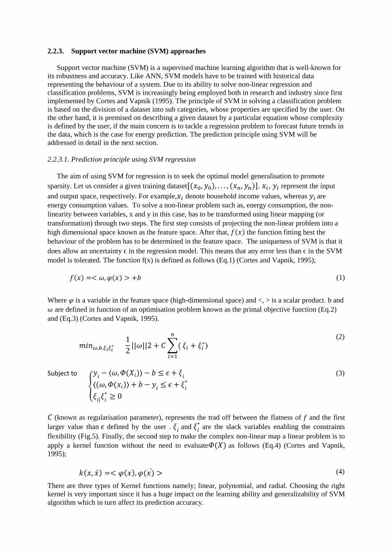
2.2.3.1. Prediction principle using SVM regression

The aim of using SVM for regression is to seek the optimal model generalisation to promote

sparsity. Let us consider a given training dataset[(𝑥0, 𝑦0), . . . , (𝑥𝑛, 𝑦𝑛)]. 𝑥𝑖, 𝑦𝑖 represent the input

and output space, respectively. For example,𝑥𝑖 denote household income values, whereas 𝑦𝑖 are

energy consumption values. To solve a non-linear problem such as, energy consumption, the non-

linearity between variables, x and y in this case, has to be transformed using linear mapping (or

transformation) through two steps. The first step consists of projecting the non-linear problem into a

high dimensional space known as the feature space. After that, 𝑓(𝑥) the function fitting best the

behaviour of the problem has to be determined in the feature space. The uniqueness of SVM is that it

does allow an uncertainty ϵ in the regression model. This means that any error less than ϵ in the SVM

model is tolerated. The function f(x) is defined as follows (Eq.1) (Cortes and Vapnik, 1995);

𝑓(𝑥) =< 𝜔, 𝜑(𝑥) > +𝑏 (1)

Where 𝜑 is a variable in the feature space (high-dimensional space) and <, > is a scalar product. b and

𝜔 are defined in function of an optimisation problem known as the primal objective function (Eq.2)

and (Eq.3) (Cortes and Vapnik, 1995).

𝑚𝑖𝑛𝜔,𝑏,𝜉𝑖𝜉𝑖∗

1

2||𝜔||2 + 𝐶 ∑(

𝑛

𝑖=1

𝜉𝑖 + 𝜉𝑖∗⟩

(2)

Subject to

{

𝑦𝑖 − ⟨𝜔, 𝛷(𝑋𝑖)⟩ − 𝑏 ≤ 𝜖 + 𝜉𝑖

⟨(𝜔, 𝛷(𝑥𝑖)⟩ + 𝑏 − 𝑦𝑖 ≤ 𝜖 + 𝜉𝑖∗

𝜉𝑖|𝜉𝑖∗ ≥ 0

(3)

𝐶 (known as regularisation parameter), represents the trad off between the flatness of 𝑓 and the first

larger value than 𝜖 defined by the user . 𝜉𝑖 and 𝜉𝑖∗ are the slack variables enabling the constraints

flexibility (Fig.5). Finally, the second step to make the complex non-linear map a linear problem is to

apply a kernel function without the need to evaluate𝛷(𝑋) as follows (Eq.4) (Cortes and Vapnik,

1995);

𝑘(𝑥, �́�) =< 𝜑(𝑥), 𝜑(𝑥)́ > (4)

There are three types of Kernel functions namely; linear, polynomial, and radial. Choosing the right

kernel is very important since it has a huge impact on the learning ability and generalizability of SVM

algorithm which in turn affect its prediction accuracy.

2.2.3.2. Applicability in the building life-cycle

Since first adopted by Dong et al. (2005) for energy forecasting until now, the use of SVM models has

been mainly confined to predicting energy consumption and temperature of individual buildings

(mostly commercial or administrative) during their operational stages (Ahmad et al., 2014). However,

recent work done by Son et al. (2015) used SVM regression models to predict the electricity

consumption of government owened buildings in the early design stages. This was achieved by first

retrieving the relevant parameters through applying a variable selection algorithm called RreliefF.

Afterwards, the SVM model was trained with an existing dataset for 175 government owned

buildings. The trained SVM could predict the energy consumption of government owned-buildings

during the design stages but with Mean Absolute Percent Error (MAPE) of 35% which means that the

SVM prediction accuracy is reasonable according to Lewis (1982) scale.

On the other hand, a lot of publications have addressed the prediction of electricity consumption

in non-residential buildings during the operational stages using SVM regression models. For

example, Lai et al. (2008) forecasted the electricity consumption of a building for a period of three

months after the SVM model had been trained with electricity consumption data measured over one

year period. The authors obtained a satisfactory match between measured and predicted data.

Similarly, Li et al. (2009) compared the prediction accuracy of a back propagation neural network

with an SVM model while forecasting the cooling load of an office building in Guangzhou in function

of outdoor dry-bulb temperature, humidity, and solar radiation. The results have shown that the SVM

model had a better prediction accuracy than the ANN model. Similar findings were reported one year

later by Li et al. (2010) after the following models namely; SVM, back propoagation neural network,

radial function neural network, and general regression neural network, have been employed to predict

the annual electricity consumption of 9 office buildings.

In an attempt to address the lack of studies applying SVM to residential buildings, Jain et al. (

2014) questioned the applicability of SVM regression models for forecatsing the energy consumption

of multi-family buildings. This was achieved by investigating the accuracy of the employed SVM

regression models in function of different temporal (hourly, daily, etc...) and spatial (whole building,

by floor, etc...) granularity of the measured electricity consumption data. Their findings suggested that

SVM can be extend to cover energy forecasting of multi-family buildings as long as the

measurements used to train the SVM model are perfomed at least at every floor and with a minimum

of 1 hour interval.

Figure 5. SVM regression function with slack variables,

observed and predicted data points (tripod, 2015)

http://www.vanguardsw.com/business-forecasting-101/mean-absolute-percent-error-mape/

2.2.3.3. Advantages of support vector machine approaches

Comparatively to existing artificial intelligence approaches, SVM for regression have shown better

results in terms of accuracy.

In contrast to aritificial neural networks, SVM for regression are less prone for over-fitting issues

due to their regularisation parameter 𝐶.

2.2.3.4. Disadvantages of SVM tools and approaches

One of the limitations of SVM for regression is the lack of universal method for selecting the

appropriate Kernel function (Yilmaz et al., 2015).

Since requiring enormous historical data and computational resources, SVM is not cost-effective

SVM for regression do not rely on 3D models, hence they are not flexible in assessing energy

conservation measures and their adoption by urban planners is complex.

2.3. Hybrid approaches

Hybrid models were first introduced in the 1990s for the purpose of improving HVAC control

systems efficiency. They are based on the idea of combining physical, statistical, and artificial

intelligence models where data samples are reasonably small, incomplete, or subject to uncertainties

(Foucquier et al., 2013).

2.3.1. Hybrid approaches’ structures and prediction processes

There exist three possible structures of hybrid approaches as shown in (Table.4). The first one

involves the estimation of optimal physical parameters with the help of machine learning algorithms

through the combination of one dimensional heat transfer models with optimisation models (Genetic

Algorithms usually). The second approach consists of describing the dwelling behaviour by

implementing a learning model through the use of statistics. Finally, the third approach, which is not

referenced in building energy prediction literature according to Foucquier et al. (2013), comprises the

employment of statistical models in areas where physical/thermodynamic models are inadequate or

inaccurate. For example, when thermal properties of a given room are unknown or when the aim is to

consider the variation in users’ behaviour.

Table 4. Possible strategies of hybrid approaches

Possible hybrid approach Approaches involved Common purpose of use

1 Engineering

Artificial intelligence

Estimation of optimal physical parameters

2 Artificial intelligence

Statistical

Describing the building thermal behaviour

3 Statistics

Engineering

Estimation of optimal physical / techno-

socioeconomic parameters which could have

been missing or inaccurate.


Hybrid models are mainly used for the estimation of optimal physical parameters and energy

consumption prediction to a lesser extent. However, despite not directly linked to energy prediction

modelling, the determination and optimisation of such parameters to achieve low-energy consumption

certainly assist urban planners in their planning strategies. This does not only apply to the design

stages but also the operational ones.

To assist energy planning in the design stages Znouda et al. (2007) coupled an energy simulation

engine, which was specifically developed for Mediterranean weather, with a genetic algorithm to

retrieve the optimum architectural and physical parameters; consequently, improve energy efficiency

in summer and winter. The strength of this approach lies in its simplicity as only few parameters are

involved. Similarly, Tuhus-Dubrow and Krarti (2010) followed almost the same process using a

different energy simulation engine (DOE-2) to determine the most efficient dwelling form(s) for

amongst U shape, L shape, T shape, H shape, trapezoidal, and rectangular across 5 different US

climatic zones. The findings suggested that the two latter shapes were the most efficient.

Hygh et al. (2012) merged statistical regression methods with building simulation tools to predict

the energy consumption of medium size rectangular shape buildings in 4 major climatic zones in the

US. It was achieved by first, investigating the range of parameters that are frequently changed at the

early design stages and likely to affect energy consumption through analysing the literature. These

parameters include, building area, number of stories, aspect ratio, orientation, roof colour, glazing

ratio, and U-values of walls and windows. Secondly, based on the possible min-max values of each

parameter, Monte Carlo method was adopted to incorporate all possible inputs probabilities and

replace default values in the referential thermal model. Thirdly, all the resulting iterations were

embedded in energy plus simulation engine using Perl script before computing the annual energy

consumption of each scenario. Afterwards, the rich database, which contains the latter and the

randomly selected values of each parameter, is generated. This was then used to develop multivariate

linear regression model. This approach has been also adopted by Asadi et al. (2014).

2.3.3. Strengths of hybrid approaches

Hybrid models are a good alternative to ANN and statistical regression models when there is a

limited number of parameters or data samples are reasonably small.

Unlike engineering methods, the hybrid ones do not require a detailed description of the building

geometry and thermal properties of the building envelop.

Their outcomes can be interpreted from a physical point of view.

2.3.4. Limitations of hybrid approaches

Hybrid models require a considerable amount of computation time and resources.

May require some support and training due to the fact that they combine two distinct approaches.

3. Urban scale tools and approaches

Urban energy forecasting models for aiding physical improvements are mostly bottom-up models

(Heiple and Sailor, 2008). This implies that the energy demand or CO2 emission of the building stock

of an urban area are forecasted in function of a representative sample usually via extrapolation.

3.1. 2D GIS based urban energy prediction models

3.1.1. Structure

GIS (geographical information system) is a complex information system that integrates, stores,

manages, analyses, interprets and visualises data, which are geo-spatially referenced, in different ways

in order to understand trends, patterns, and relationships. This section will focus solely on the

structure of urban energy forecasting approaches that utilise 2D GIS tools. In general, the majority of

these approaches, despite their diversity, are composed of the following components;

Inputs: comprise variables which describe the physical and thermal characteristics of the

dwellings in addition to standard occupational schedules data. (Table.5) represents a list of the

most common variables for this approach based on some important examples from the literature

and highlights possible sources from which these inputs are derived.

Assumptions: usually apply for some variables related to occupants’ behaviour as well as

thermal characteristics of the buildings such as, household size, patterns of heating, and level of

insulation.

Baseline models: The estimation of energy consumption at the urban scale (in a bottom up

fashion) is produced with the help of baseline models which are usually physically based ones,

such as BREDEM (the Building research establishment domestic energy model). The inputs

requirements and complexity of energy prediction varies from one baseline model to another

(Kavgic et al., 2010).

Calculation engine: is the software in which baseline models or algorithms are incorporated to

perform energy consumption calculations such as, SBEM (simplified building energy model).

Data exchange module: allows the exchange of data between the GIS platform and calculation

engine such as, dynamic data exchange (DDE).

GIS platform: Although it provides certain geometric inputs, a GIS platform is mainly dedicated

to visualising the energy consumption or CO2 emission of buildings using thematic mapping

techniques (Jones et al., 2001); (Jones et al., 2007); (Batty, 2007).


Generally speaking, the process begins with determining the type of the baseline model and its

calculation engine based on the aim of prediction, availability of data inputs, envisaged accuracy, time,

and availability of resources as shown in (Fig.6) . Once determined, although not necessary if it is

available, data will be collected using various methods ranging from quick inspection surveys to

detailed energy audits depending on the decisions made in the previous stage. After that, the

geometric variables extracted from GIS (e.g. building area) along with the collected data will be

inserted to perform the calculation. This will be followed by a validation process that will compare the

outcomes with existing databases such as regional statistical data (top-down consumption data). If

there is not a good agreement between both datasets, inputs will be adjusted accordingly. Finally, with

the help of data exchange module, GIS platform will automatically geolocate and visualise the outputs

on the 2D map of the studied urban area.


2D GIS based tools are mainly employed in the operational phases of the building lifecycle to

estimate and compare the energy consumption or CO2 emission of building areas before and after

physical improvement measures (e.g. renewable resources, retrofit, etc…) have been applied.

Furthermore, to determine building areas with potential energy savings. For example, Jones et al.

(2001) estimated the annual energy consumption of Neath Port Talbot residential sector, UK, in

function of a representative sample composed of 100 archetypes of dwellings. After that, certain

physical measures included in the UK home energy conservation act (HECA) such as, water tank

insulation, were applied to the archetypes whose energy consumption values were re-estimated

accordingly. Finally, the archetypes were extrapolated in GIS to thematically visualise the energy

consumption and CO2 emission of the whole residential sector before and after physical

improvements. Similarly, Heiple and Sailor (2008) estimated the energy consumption of the building

stock in Houston, USA in function of 30 archetypes composed of 8 dwellings and 22 commercial

buildings. Secondary databases, more precisely residential energy consumption survey (RECS) and

GIS lot tax database, were used to retrieve geometric parameters, thermal characteristics, and age of

buildings. After the total energy consumption had been calculated using a building simulation tool

eQUEST based on the retrieved parameters, the outcomes were mapped into a GIS platform to

visualise the hourly energy consumption at 100 m grid resolution.

2D GIS based approaches have been also highly associated with renewable energy planning in the

literature. For instance, Aydin et al. (2013); Janke, (2010); Connolly et al. (2010) adopted 2D GIS to

identify suitable areas for solar and wind farms, as well as pumped storage hydro plants. Kucuksari et

al. (2014) has recently suggested a framework integrating 2D GIS, optimisation algorithms, with

simulation engines to assist the placement and dimensioning of solar panels in dense urban areas. In

addition to that, 2D GIS approaches played a major role in evaluating the benefit of expanding district

heat systems in certain studies (Nielsen and Möller, 2013).

3.1.4. Advantages of 2D GIS based approaches

Have a potential of being integrated into urban planners’ everyday life, since GIS tools are

increasingly being adopted in urban planning.

They are good for analysing and communicating potential renewable energy areas.

3.1.5. Disadvantages of 2D GIS based approaches

There is a lack of universal guidelines on the processes, nature, and granularity of parameters

involved in this approach.

Energy forecasting using 2D GIS based approaches require a considerable amount of

computation time of resources since they reply on building simulation tools.

Figure 6.Conventional prediction process of 2D GIS based urban energy planning

and prediction models

Table 5. Common inputs for 2D GIS-based energy forecasting approaches and their corresponding derivation

sources.

Authors Inputs Category of

inputs Source

(Rylatt et al., 2003); Wind speed

Weather data

-Data from metrological

stations or;

-Onsite measurements

(Kavgic et al., 2010);

(Heiple and Sailor,

2008); (Rylatt et al.,

2003);

Heating/cooling degree day


(Heiple and Sailor,


2003); (Jones et al.,


2007)

Building-age Building-age

-Official surveys (e.g.

English house condition

survey)

-Existing maps / site

inspection

Building typology (e.g. detached,

semi-detached, etc...) Typology -Site inspection, existing

maps

exposed perimeters

Building

geometry

-GIS tools or;

-Building footprints

from existing maps and ;

-Building typology and

ages

roof and wall areas

Building volumes

Façade orientation

U-values for roof, external walls,

Thermal

characteristics

-Assumptions

-Official surveys based

on Building age and

typology or;

-Energy audits

Type and thickness of insulation

Window area and glazing ratio

Thermal zones and their U-Values


(Heiple and Sailor,


2003);(Jones et al.,


2007)

Type of boiler, number of pumps and

fans, size and insulation of hot water

tank, insulation of pipes, type of

controls, solar panel area (if

available).

HVAC system

specification

-From building

regulations based on age

and typology of the

building

-Energy audits

-Assumptions


(Heiple and Sailor,




2007)

Number of occupants, temperature of

each building zone, heating hours,

etc…

Internal gain and

occupancy

schedules

-Assumption

-Official surveys

3.2. CityGML (3D GIS) based urban energy prediction models

Recently, there has been a shift in focus from conventional 2D GIS urban energy planning models

towards CityGML (3D GIS) based ones. This is owing to the growing interest in 3D CityGML

models and their applications (Krüger and Kolbe, 2012); (Gröger and Plümer, 2012).CityGML is an

XML object-oriented information modelling approach for representing, storing and sharing 3D city

model data. It provides the standard mechanisms that govern the description of different 3D objects in

relation to their geometry, semantics, and topology. It is equipped with 10 core thematic modules

including building, vegetation, relief, and others as illustrated in (Fig.7). However, other features such

as, the ones related to energy forecasting can be added through application domain extensions (ADE).

The building module, which is the backbone of CityGML, permits the geometric as well as

semantic representation of buildings and their elements (Kolbe et al., 2005). Each Building in

CityGML possess the following attributes namely; class, address, usage, function, roof type, building

height, number of floors, year of construction, year of demolition, and cross-reference number, in

which the three later attributes are shared between all types of buildings and their components. The

cross-reference number facilitates the update of objects’ features and also the extraction of additional

information from other databases. Apart from sematic properties, the geometric description of the

building module is built upon the GML 3.1.1 Model (ISO 19107) developed by Cox et al. (2002).

Therefore, buildings can be represented as solid or multisurface geometry. However, the former is

more preferable for energy related applications since the calculation of volumes is a straightforward

task (Gröger and Plümer, 2012).

One advantage of CityGML over other city 3D modelling approaches is its flexible discrete level

of detail (LOD) which is not only confined to geometric but also sematic characteristics (Chalal and

Balbo, 2014). However, since the granularity of geometric as well as semantic information varies

from one LOD to another, the chosen level detail(s) influence the energy prediction accuracy. For

instance, a building with a gabled roof in LOD1 is represented as a block resulted from the extrusion

of its footprint with a flat roof surface, whereas in LOD2, it processes a rough gabbled roof structure,

which certainly has an impact on the building heated volume calculation.

The wide adoption of BIM 3D models in the architecture, engineering, and construction industry in

addition to the widespread of 3D GIS systems over last few years, have led a lot of researchers to

investigate the interoperability between IFC ( industry foundation class) and CityGML (Hijazi et al.,

2009); (Mignard and Nicolle, 2014). This will be subsequently discussed in more detail in the 3.2.1.

3.2.1. Interoperability between CityGML and IFC

There exist three distinct approaches to interoperability between CityGML and IFC namely;

unidirectional conversion, unifying approaches (Bi-directional conversion), and approaches based

on extending the CityGML models (Table.6).

The first one consists of exchanging information between both standards in a unidirectional

fashion, meaning from IFC to CityGML or vice-versa. Please note that unidirectional conversion

from CityGML to IFC is beyond the scope of this article, please refer to the work of Nagel et al.

(2009). Unidirectional conversion from IFC to CityGML is the most addressed in the literature and

widely supported by some commercial software packages such as FME (feature manipulation

software) or GeoKettle. However, none of them has the ability to generate 3D building models

which comply geometrically and/or semantically with CityGML standards (Donkers et al., 2015).

This is owing to the structural differences between IFC and CityGML which cause a lot of loss of

information during the conversion process. Another drawback of this approach is that the geometric

conversion to high CityGML level of detail (mainly LOD3, LOD4) is still challenging and require

extensive post-processing as well as users’ judgement (Delgado et al., 2013) ; (Boyes et al., 2015).

For example, in (Fig.8), which depicts the conversion of a roof and slabs from IFC to CityGML, it is

clear that a slab in IFC is represented as a solid object and defined by an IFC class (ifcSlab), whereas

in CityGML, it is composed of two surfaces classified under CeillingSurface and FloorSurface, or

GroundSurface. The upper surface is considered as floor surface for the upper building level,

whereas the lower one, represents a ceiling surface or ground surface for the lower building level.

As for CityGML Roof, the upper surface is a roof surface, whereas the lower one is a ceiling surface

for the below storey (El-Mekawy et al., 2011).

On the other hand, some researchers like El-Mekawy et al. (2011); Xu et al. (2014) tried to

bridge the interoperability gap of unidirectional conversion approaches by integrating BIM with

CityGML. This approach is often referred to as unifying information model or Bi-directional

conversion in the literature. However, it is still fairly at the conceptual stages and has not been

implemented yet (Amirebrahimi et al., 2015).

The third approach, which relies on extending CityGML model, can be performed in two distinct

ways namely; 1) generic objects and attributes 2) application domain extension (ADE) mechanism.

The first method consists of using generic objects to model and exchange features which are not

predefined by existing CityGML thematic classes (e.g. walls). However, this method is limited due

to the objects nomenclature conflicts it can create between CityGML users. Furthermore, the

difficulty of validating the occurrences and layout of generic objects/ attributes by XML parsers (El-

Mekawy et al., 2011). Conversely, the second method relies on application domain extension (ADE)

in either introducing new properties to existing CityGML classes (e.g. household size) or defining

new object types. For example, the GeoBIM extension developed by Van Berlo (2009) does not

only add new classes to CityGML (e.g. Stair class) but also new IFC properties such as, width and

height, to existing CityGML classes including windows, room, building, and door. The advantage

of ADE over generic objects is that the former overcome the nomenclature limitation of generic

objects as it is defined within an additional XML schema definition file with its own namespace

(Gröger et al., 2012). However, despite this benefit, embedding information from IFC through ADE

CityGML extension can result in large file formats as claimed by (El-Mekawy et al., 2011).

Nevertheless, ADE is the first choice strategies for certain applications such as urban energy

planning.

Table 6. Strengths and limitations of different interoperability approaches between IFC and CityGML

Approach Approach

Principle

Relevant

Example Strengths Weaknesses

Approach

1

- Unidirectional

conversion from

IFC to

CityGML

(Nagel and

Kolbe,

2007)

(Isikdag and

Zlatanova,

2009)

(Nagel et al.,

2009)

-Widely Supported by

commercial software

packages.

-Benefit urban planning

applications.

-Loss of information.

-Conversion to lower LOD

(LOD1, LOD2).

-Focused on geometric

transformation issues.

-Extensive post-processing is

needed.

Approach

2

unifying

approaches (Bi-

directional

conversion)

(El-Mekawy

et al., 2011)

(Xu et al.,

2014)

-Intends to bridge the

interoperability gap between

IFC and CityGML.

-Remains fairly at the

conceptual stages.

Approach

3

Extending the

CityGML model

by either;

A. Introduction

of generic

city objects.

(Gröger et

al., 2012)

-Ability to model and

exchange new features in

CityGML.

- Nomenclature issues.

-The validation of generic

objects and attributes represent

an issue for XML parsers.

B. Using

Application

extension

domain

(ADE)

(Van Berlo,

2009)

-Defined with an additional

XML schema to avoid

nomenclature conflicts.

-Widely adopted for urban

energy planning applications.

-Massive file size

-The combination of different

ADE modules is not possible

3.2.2. Structure of 3D GIS (CityGML) models

Apart from the 3D thematic visualisation, energy ADE, the employed baseline models (described

below), most 3D CityGML urban prediction models consist of a similar structure to the 2D GIS ones.

Energy prediction models: are the algorithms used in the calculation of energy consumption of

dwellings (mainly for space heating). Beside recent studies that utilised building energy

simulation tools such as IESVE, researchers in this field tend to frequently employ steady –state

energy balance prediction models such as; quasi-state model (ISO/FDIS 13790) (Corrado et al.,

2007); (Nouvel et al., 2013); or DIN V 18599 (Strzalka et al., 2011).

Calculation engine: unlike 2DGIS models and very recent studies in this area, Excel-based

simulation tools incorporating steady-state energy balance algorithms such as, Fraunhofer-IBP or

EnerCalC, are used calculate the energy consumption of dwellings.

Figure 7.CityGML modules

Figure 8. Unidirectional conversion of roof and slabs from IFC to CityGML (El-Mekawy et al., 2011)

Energy ADE: it facilitates the integration of energy indicator and indexes into CityGML models.

In the well-known energy ADE developed by Krüger and Kolbe (2012) for instance, this

integration is performed in two distinct ways. First, elementary indicators variables such as,

number of accommodation units, are directly retrieved from buildings’ semantic properties.

Secondly, complex indicators values (e.g. heated volume) are defined using complex functions.

Further indicators such as, assignable area, can also be obtained from elementary indicators and

other complex indicators. Recently, the international consortium of urban energy simulation has

recently called for the development of a universal energy ADE (SIG3D, 2015).


In contrast to studies on 2D GIS prediction models, it has been noticed that the choice of

prediction models and data collections procedures has not been explicitly addressed. This is believed

to be due to the influence of two studies that endeavoured to define standard or universal inputs for

this type of models. These are the energy atlas of Berlin study conducted by Krüger and Kolbe (2012)

and the model developed by Carrión et al. (2010). For these reasons and other related to the

familiarity with data collection methods pertaining to these standard parameters, it is believed that a

conventional prediction pipeline begins with acquiring data as demonstrated in (Fig.8). Dwellings

heights, footprints, and type are usually obtained from GIS or digital cadastral databases, whereas

energy consumption values are provided by utility companies. Year of construction, on the other hand

is usually obtained from historical sources (e.g. raster maps). If 3D CityGML models covering the

pilot area are not available, the next step consists of generating a sematic CityGML model following

two possible strategies. First, different formats of 3D city models can be exported to CityGML format.

However, due to the lack or loss of sematic information after the format conversion process occurred,

the exported model is subject to a pre-processing phase embedding all the collected data and fixing

issues related to geometry. The second strategy is to create a CityGML sematic model from scratch

using one or a combination of different modelling techniques such as laser scanning and LIDAR,

depending on the envisaged LOD and prediction’s accuracy (Nouvel et al., 2013). This can be time

consuming and challenging for models with LOD2 or above. After creating a CityGML model, with

the help of ADE energy, further inputs such as, assignable area, are first obtained from the buildings

geometry and exiting inputs, then integrated into the model. Once these parameters are embedded,

dwellings with similar age and size are grouped into archetypes. After assumptions covering thermal

parameters (e.g. U-values) are made based on the age and size, the calculation of energy

consumption, in most cases the space heating demand, of these archetypes is performed. This is

achieved with excel-base software supporting steady-state energy balance models. Afterwards, the

outputs are validated against existing energy consumption values and if necessary certain adjustments

to the inputs until a good match is achieved. Finally, the outputs are transferred to the 3Dcitygml

model with the help of a data exchange module to be thematically visualised.


CityGML based approaches have been mainly used in the operational phases of the building life-

cycle. More precisely, to target building areas with retrofits potentials through diagnosing their

heating demand (Nouvel et al., 2014). However, recently their applicability has been extended to

cover the identification as well as assessment of renewable energy potentials across building areas

(Saran et al., 2015).

For example, Carrión et al. (2010) suggested an approach to easily assess potential refurbishment

in building areas. This was first achieved by deriving parameters such as, storey heights and building

age from the German cadastral information system as well as scanned raster maps, respectively. Other

parameters such as, building volume, building height, assignable area, the surface- to-volume ratio,

were extracted from the atlas of Berlin CityGML model either directly or indirectly using functions.

Once these parameters were obtained, the heating energy consumption of the building area has been

statistically calculated in excel based simulation tool using a degree day model. Finally, the results

were then compared to consumption values from existing building libraries based on the building age

and typology. Similar methodology and process have been applied to areas in cities like Stuttgart,

Hamburg, Ludwigsburg, and Lyon in the work of Krüger and Kolbe (2012); Nouvel et al. (2013);

Bahu et al. (2013); Strzalka et al. (2011) with the exception of the study of Kaden and Kolbe (2013)

who extend the capabilities of this approach to cover electricity and hot water consumption in

residential areas. The estimation of electricity power demand was achieved by assigning the mean

electricity values published by Vattenfall utility company to each household in the building based on

their size while presuming that all of them possess similar appliances.

On the other hand, few studies have focused on exploring the potential(s) of CityGML in assisting

renewable energy planning. For instance, Alam et al. (2012) proposed a method to assess the

performance of PV systems through simulating roof shading analysis for direct radiation inside a

CityGML 3D model. This method, which is similar to ray tracing in CAD rendering engines,

comprises first triangulating all roofs’ surfaces and drawing straight lines from their centroids towards

the sun direction. The second step consists of checking intersections between the sun ray vector and

other roof surfaces. Any triangle containing an intersection means that is shaded. After that, shaded

triangles were combined to represent the overall shaded roof area. Conversely, Saran et al. (2015)

addressed the evaluation of PV systems from a completely different perspective by proposing a new

approach built upon incorporating building energy simulation tools outputs into CityGML, (Fig.9).

This was accomplished by first, generating a 3D CAD model using conventional CAD tools, in

function of collected geometric parameters (e.g. Footprints) using total station surveys as well as

satellite maps. Secondly, the CAD model was converted into a CityGML model with the help of

feature Manipulation Engine (FME) converter. Similarly, a thermal model containing thermal zones,

external/ internal walls, windows etc… was created from the CAD model using gModeller-Energy

Analysis Sketchup Plug-in and then exported as a gbxml file. Thirdly, the solar gain of different

building parts (roofs and walls), was simulated using Suncast module in IESVE while considering

shading surfaces, orientation, and seasonal changes. The outputs were then stored in a PostGIS

database to perform semantic queries such as, where should PV systems be installed to generate 5

MW of power per annum? With the help of query filter expression in java, CityGML displays only

the building components with matching values.

Figure 9.Conventional prediction process of 3D CityGML approaches

3.2.5. Advantages of CityGML based planning and forecasting approaches

Unlike other city 3D model formats, CityGML has the ability to model and represent objects in

different level of detail(s) LOD geometrically and semantically.

CityGML approaches have shown lot potentials for the estimation of heating energy

consumption.

3.2.6. Disadvantages of CityGML based approaches

Their prediction accuracy relies heavily on the availability and quality of data obtained from

municipalities as well as onsite measurements (Nouvel et al., 2014).

3D CityGML models for a particular city/region are not applicable to another since their

development is mostly achieved using non-standardised data structure specified locally.

The interoperability between CityGML LOD3/ LOD4 and other standards like IFC is still

challenging and require extensive post-processing (Zhu and Mao, 2015).

The potential of 3D CityGML models is not fully utilised for energy prediction applications.

Indeed, they are mainly dedicated for visualisation purposes except providing certain geometric

inputs.

3.3. Bottom-up statistical methods

Statistical bottom-up methods are based on correlating energy consumption/indexes with

influencing factors, mostly weather parameters. This is usually achieved by applying different

regression analyses, either linear or multivariate, to sufficient historical performance data (usually

energy bills data), although Bayesian and Monte Carlo based approaches could be also employed

Figure 10. The prediction process adopted by Saran

et al. (2015)

(Fumo and Rafe Biswas, 2015a). However, historical performance data must have a high level of

statistical significance to meet the accuracy requirements of energy planning (Pedersen, 2007). Indeed,

this is evident in the work of Cho et al. (2004) in which the developed regression models on the basis

of 1day, 1 week, 3 months measurements resulted in errors in the prediction of annual energy

consumption of 100%, 30%, and 6%, respectively. For this reason in addition to their ability to handle

big data sets, statistical approaches are mostly employed at the urban scale. However, their

applicability can be extended to cover the building scale as well.


After being trained with large samples of hundreds or thousands of dwellings, statistical methods

can be employed to estimate the energy consumption of entire dwellings or the thermal characteristics

of their components in function of influencing parameters (Foucquier et al., 2013). Such factors are

not only prominent for the evaluation of buildings energy performance but also the assessment of

energy management strategies or saving potentials during commissioning (Ghiaus, 2006). For

example, energy signature, which is best fit straight line correlating energy consumption with climatic

variables, was adopted by Belussi and Danza (2012) for two main purposes. The first one is to check

the conformity of certain buildings energy performance at the operational phases against the one

estimated at the design phase as shown in (Fig.10). On the other hand, the second aim consists of

determining potential savings through the comparison of their energy signature models in the

operational phase with the one in accordance with building regulations.

As for determining thermal characteristics, Jiménez and Heras (2005) for instance, compared the

accuracy of two regression models namely; single output and a multi-output auto regression with

extra inputs, in predicting the U- as well as G values of few buildings’ components. The results of

latter model had a better agreement with the measured values in comparison to the former.

Furthermore, the predicted values of windows in both models were more accurate than the ones of the

walls. Fumo and Rafe Biswas (2015) assessed as well as compared the quality of simple linear and

multiple regression models corresponding to the energy consumption of an unoccupied demonstration

house in function of weather parameters. The authors concluded that the more time interval is

allowed between observed data, the better regression model quality is obtained, regardless of the

nature of the employed regression model. Similarly, Richalet et al. (2001) presented an assessment

methodology for single family dwellings which consists of deriving the thermal characteristics

through the development of building energy signatures using continuous onsite measurements. Those

thermal parameters are then used to determine a normalised heating annual consumption based on

standards occupant schedule and weather conditions. However, despite the authors’ intention to

distinguish the impact of occupants’ behaviour from climatic influences by evaluating occupied and

unoccupied dwellings, the potential of onsite measurement was not utilised for this purpose. Instead,

standard EU internal gains values and occupants schedules were employed for all dwellings.

Therefore, errors in the estimation of normalised annual energy consumption were superior to 20% for

some occupied dwellings.

3.3.2. Advantages of bottom-up statistical methods

Unlike engineering approach, the statistical one do not depend on the 3D geometry of the

building since it is not based on thermodynamic models (Foucquier et al., 2013).

In comparison to other prediction methods, statistical models are the easiest to develop (Zhao and

Magoulès, 2012).

Statistical methods have a great ability to recognise and model the variation in households’

energy behaviour (Swan and Ugursal, 2009).

3.3.3. Disadvantages of bottom-up statistical methods

Since statistical approaches rely primarily on historical data, their adoption is impractical when

data is unavailable or cannot be measured.

Statistical methods are less accurate than other approaches. Furthermore, their ability to evaluate

the impact of physical improvements is limited (Swan and Ugursal, 2009).

4. Discussion

This article has extensively reviewed different energy planning and forecasting approaches

supporting physical improvement strategies in the building sector. This analysis was performed in

accordance with their structure, conventional prediction pipeline, advantages and limitations, while

providing some relevant examples on their applicability in the building life cycle (Table.7).

At the building scale, Engineering methods, which rely heavily on buildings 3D models and

energy simulations tools, are characterised by their flexibility, user-friendliness, high integration with

the majority of CAD/BIM tools, and comprehensive outputs. However, the large number of inputs

requirement and involvement of calibration procedures to generate accurate results in certain projects,

represents their major drawbacks. Nevertheless, they are still first choice methods for physical

interventions at this scale. On the other hand, artificial intelligence energy prediction models in

general, ANN and SVM particularly, do not rely on 3D models to proceed and can generate accurate

estimations due to their great ability to handle non-linear and complex processes. However, since

trained with large amount of historical data, they are impractical when these datasets are unavailable

or their size is small. Furthermore, unlike engineering models, their main disadvantage is the lack of

generalizability of their algorithms to represent the wider sample of dwellings at the urban scale. In

other words, even if certain changes have been applied to the same building envelop, its HVAC

system, or even occupancy, the employed artificial intelligence model has to be re-trained from

scratch. Therefore, they are not time and cost effective approaches to adopt in urban energy planning

given the imposed strict CO2 emission targets. Conversely, Grey box (Hybrid) models, which

combine the strengths and eliminate the weaknesses of the above approaches in addition to statistical

ones, are well known for their great ability to handle problems related to small samples and missing

data. Thus, it could be possible to utilise them in urban energy planning when certain parameters,

especially the thermal ones (e.g. U-values, glazing ratio, etc…), are unattainable.

Figure 11 depicts a comparison between the design and real (operational)

signature models by Belussi and Danza (2012). It is clear that behaviour of

building during the operational stage is different from the design one since both

curves are not overlapping.

Table 7 Summary of the reviewed approaches

Frequent

Intervention

scale

Approaches Require

3D

models?

Require

historical

data?

Easy to

employ?

Prediction

accuracy

Applicability in

the building

life-cycle

Building scale

Engineering Yes No Easy to

moderate

depending

on the

complexity

of the

simulation

tool.

Fair to

High

Multi stages

including

Design,

operational, and

maintenance

stages

ANN No Yes No high Mostly

operational

stages

Very limited for

design phases

SVM No Yes No Fairly high Mainly

operational

stages

Very limited for

design phases

Hybrid Yes, if

engineering

methods

are

involved

Yes,

partially

No Fairly high Design and

operational

stages

Urban scale

2D GIS Yes but not

necessarily

No Moderate Fair Operational

stages

3D

CityGML

Yes No Moderate Fair to

High

Operational

stages

Bottom-up

statistical

No Yes Yes Fair Operational and

maintenance

stages

As for the urban scale, the analysis of the 2D GIS and 3D CityGML based energy prediction

approaches have shown a great integration potential in the everyday’s life of urban planners since GIS

tools are increasing being adopted in urban planning. Furthermore, it has outlined the similarities

between both approaches’ processes and visualisation patterns, except the 3D environment, energy

application domain extensions (ADE), and discrete level of detail for 3D CityGML. This clearly

indicates that there is a major problem in the shift from 2DGIS to 3D GIS approaches. Indeed, what is

the point of investing more time or maybe resources in using 3D CityGML for energy prediction if the

2DGIS ones can perform exactly the same task? It is believed that answer to this question is related to

the fact that the great potentials of 3D CityGML models are not fully utilised yet for energy prediction

applications at the urban scale. This evident in the majority of work on 3D CityGML heating demand

analysis models which exist only in LOD1 or LOD2 at most, although the minimum level of detail

requirement for this particular purpose should be LOD3. This is simply because LOD1 and LOD2 do

not contain openings and protruding building elements such as, shading devices, which certainly

affects their prediction accuracy. Another problem is the independence of 3DCityGML and 2GIS

models from energy calculation engines. In fact, both GIS and 3D CityGML models are only

employed as visualisation platforms despite providing few geometric inputs. Finally, although

bottom-up statistical approaches do rely on historical data to solve linear problems and have fair

prediction accuracy, they are adequate tools for quick buildings energy performance inspection at the

urban scale. Furthermore, they have a great ability to discern impact of occupancy on building energy

consumption. Therefore, their adoption is indispensable in urban energy planning.

This article has undoubtedly highlighted a lot of gaps and issues with regards energy planning and

forecasting tools that are used both at the micro as well as macro level. Among them, it is very

interesting to mention that despite the wide adoption of CityGML urban planning applications

including energy planning, most of the energy simulations are performed outside a CityGML

environment in an excel based software or building energy simulation tools (e.g. IESVE). This is a

major problem because the forecasted energy performance of buildings at the urban scale using this

approach does not consider the effect of buildings on each other (including shading effect, wind

effect, etc…). Therefore, we strongly recommend the development of an energy simulation plugin

embedded in CityGML environment. So that the full potential of 3D models in exploited and accurate

predictions are obtained.

References

Ahmad, A.S., Hassan, M.Y., Abdullah, M.P., Rahman, H.A., Hussin, F., Abdullah, H., Saidur, R., 2014. A review on

applications of ANN and SVM for building electrical energy consumption forecasting. Renew. Sustain. Energy Rev.

33, 102–109.

Alam, N., Coors, V., Zlatanova, S., Van Oosterom, P.J.M., 2012. Shadow effect on photovoltaic potentiality analysis using

3D city models, in: XXII ISPRS Congress, Commission VIII, Melbourne, Australia, 25 August-1 September 2012;

IAPRS XXXIX-B8, 2012. International Society for Photogrammetry and Remote Sensing (ISPRS).

Al-Tamimi, N.A., Fadzil, S.F.S., 2011. The Potential of Shading Devices for Temperature Reduction in High-Rise

Residential Buildings in the Tropics. 2011 Int. Conf. Green Build. Sustain. Cities 21, 273–282.

doi:http://dx.doi.org/10.1016/j.proeng.2011.11.2015

Amirebrahimi, S., Rajabifard, A., Mendis, P., Ngo, T., 2015. A Data Model for Integrating GIS and BIM for Assessment and

3D Visualisation of Flood Damage to Building. Locate 15, 10–12.

Asadi, S., Amiri, S.S., Mottahedi, M., 2014. On the development of multi-linear regression analysis to assess energy

consumption in the early stages of building design. Energy Build. 85, 246–255.

Attia, S., Gratia, E., De Herde, A., Hensen, J.L.M., 2012. Simulation-based decision support tool for early stages of zero-

energy building design. Energy Build. 49, 2–15. doi:http://dx.doi.org/10.1016/j.enbuild.2012.01.028

Aydin, N.Y., Kentel, E., Sebnem Duzgun, H., 2013. GIS-based site selection methodology for hybrid renewable energy

systems: A case study from western Turkey. Energy Convers. Manag. 70, 90–106.

doi:http://dx.doi.org/10.1016/j.enconman.2013.02.004

Aydinalp, M., Ismet Ugursal, V., Fung, A.S., 2002. Modeling of the appliance, lighting, and space-cooling energy

consumptions in the residential sector using neural networks. Appl. Energy 71, 87–110.

doi:http://dx.doi.org/10.1016/S0306-2619(01)00049-6

Aydinalp-Koksal, M., Ugursal, V.I., 2008. Comparison of neural network, conditional demand analysis, and engineering

approaches for modeling end-use energy consumption in the residential sector. Appl. Energy 85, 271–296.

doi:http://dx.doi.org/10.1016/j.apenergy.2006.09.012

Bahu, J.M., Koch, A., Kremers, E., Murshed, S.M., 2013. Towards a 3D spatial urban energy modelling approach, in: ISPRS

Annals of the Photogrammetry, Remote Sensing and Spatial Information Sciences. Proceedings of the ISPRS 8th 3D

GeoInfo Conference & WG II/2 Workshop. pp. 33–41.

Batty, M., 2007. Planning support systems: progress, predictions, and speculations on the shape of things to come.

Belussi, L., Danza, L., 2012. Method for the prediction of malfunctions of buildings through real energy consumption

analysis: Holistic and multidisciplinary approach of Energy Signature. Cool Roofs, Cool Pavements, Cool Cities,

Cool World 55, 715–720. doi:http://dx.doi.org/10.1016/j.enbuild.2012.09.003

Boyes, G., Thomson, C., Ellul, C., 2015. Integrating BIM and GIS: Exploring the use of IFC space objects and boundaries.

Carrión, D., Lorenz, A., Kolbe, T.H., 2010. Estimation of the energetic rehabilitation state of buildings for the city of Berlin

using a 3D city model represented in CityGML. Int. Arch. Photogramm. Remote Sens. Spat. Inf. Sci. 38, 31–35.

Chalal, M.L., Balbo, R., 2014. Framing Digital Tools and Techniques in Built Heritage 3D Modelling: The Problem of Level

of Detail in a Simplified Environment. Int. J. Constr. Environ. 4.

Cho, S.-H., Kim, W.-T., Tae, C.-S., Zaheeruddin, M., 2004. Effect of length of measurement period on accuracy of predicted

annual heating energy consumption of buildings. Energy Convers. Manag. 45, 2867–2878.

Clarke, J.A., 2001. Energy simulation in building design. Routledge.

Coakley, D., Raftery, P., Keane, M., 2014. A review of methods to match building energy simulation models to measured

data. Renew. Sustain. Energy Rev. 37, 123–141. doi:http://dx.doi.org/10.1016/j.rser.2014.05.007

Connolly, D., MacLaughlin, S., Leahy, M., 2010. Development of a computer program to locate potential sites for pumped

hydroelectric energy storage. Energy 35, 375–381.

Corrado, V., Mechri, H.E., Fabrizio, E., 2007. Building energy performance assessment through simplified models:

application of the ISO 13790 quasi-steady state method, in: Proceedings of Building Simulation. pp. 79–86.

Cortes, C., Vapnik, V., 1995. Support-vector networks. Mach. Learn. 20, 273–297. doi:10.1007/BF00994018

Cox, S., Cuthbert, A., Daisey, P., Davidson, J., Johnson, S., Keighan, E., Lake, R., Mabrouk, M., Margoulies, S., Martell, R.,

2002. OpenGIS® Geography Markup Language (GML) Implementation Specification, version.

Delgado, F., Martínez-González, M.M., Finat, J., 2013. An evaluation of ontology matching techniques on geospatial

ontologies. Int. J. Geogr. Inf. Sci. 27, 2279–2301.

Dombaycı, Ö.A., 2010. The prediction of heating energy consumption in a model house by using artificial neural networks

in Denizli–Turkey. Adv. Eng. Softw. 41, 141–147. doi:http://dx.doi.org/10.1016/j.advengsoft.2009.09.012

Dong, B., Cao, C., Lee, S.E., 2005. Applying support vector machines to predict building energy consumption in tropical

region. Energy Build. 37, 545–553.

Donkers, S., Ledoux, H., Zhao, J., Stoter, J., 2015. Automatic conversion of IFC datasets to geometrically and semantically

correct CityGML LOD3 buildings. Trans. GIS n/a–n/a. doi:10.1111/tgis.12162

Ekici, B.B., Aksoy, U.T., 2009. Prediction of building energy consumption by using artificial neural networks. Adv. Eng.

Softw. 40, 356–362. doi:http://dx.doi.org/10.1016/j.advengsoft.2008.05.003

El-Mekawy, M., Östman, A., Shahzad, K., 2011. Towards interoperating CityGML and IFC building models: a unified

model based approach, in: Advances in 3D Geo-Information Sciences. Springer, pp. 73–93.

Foucquier, A., Robert, S., Suard, F., Stéphan, L., Jay, A., 2013. State of the art in building modelling and energy

performances prediction: A review. Renew. Sustain. Energy Rev. 23, 272–288.

doi:http://dx.doi.org/10.1016/j.rser.2013.03.004

Fumo, N., 2014. A review on the basics of building energy estimation. Renew. Sustain. Energy Rev. 31, 53–60.


Fumo, N., Rafe Biswas, M.A., 2015a. Regression analysis for prediction of residential energy consumption. Renew. Sustain.

Energy Rev. 47, 332–343. doi:http://dx.doi.org/10.1016/j.rser.2015.03.035

Fumo, N., Rafe Biswas, M.A., 2015b. Regression analysis for prediction of residential energy consumption. Renew. Sustain.

Energy Rev. 47, 332–343. doi:http://dx.doi.org/10.1016/j.rser.2015.03.035

Ghiaus, C., 2006. Experimental estimation of building energy performance by robust regression. Energy Build. 38, 582–587.

doi:http://dx.doi.org/10.1016/j.enbuild.2005.08.014

Gröger, G., Kolbe, T., Nagel, C., Häfele, K.-H., 2012. OGC City Geography Markup Language (CityGML) En-coding

Standard. Ogc. doi:OGC 12-019

Gröger, G., Plümer, L., 2012. CityGML – Interoperable semantic 3D city models. ISPRS J. Photogramm. Remote Sens. 71,

12–33. doi:http://dx.doi.org/10.1016/j.isprsjprs.2012.04.004

Ham, Y., Golparvar-Fard, M., 2015. Mapping actual thermal properties to building elements in gbXML-based BIM for

reliable building energy performance modeling. Autom. Constr. 49, Part B, 214–224.

doi:http://dx.doi.org/10.1016/j.autcon.2014.07.009

Heiple, S., Sailor, D.J., 2008. Using building energy simulation and geospatial modeling techniques to determine high

resolution building sector energy consumption profiles. Energy Build. 40, 1426–1436.

doi:http://dx.doi.org/10.1016/j.enbuild.2008.01.005

Hijazi, I., Ehlers, M., Zlatanova, S., Isikdag, U., 2009. IFC to CityGML transformation framework for geo-analysis: a water

utility network case, in: 4th International Workshop on 3D Geo-Information, 4-5 November 2009, Ghent, Belgium.

Hygh, J.S., DeCarolis, J.F., Hill, D.B., Ranjithan, S.R., 2012. Multivariate regression as an energy assessment tool in early

building design. Build. Environ. 57, 165–175.

Isikdag, U., Zlatanova, S., 2009. Towards defining a framework for automatic generation of buildings in CityGML using

building Information Models, in: 3D Geo-Information Sciences. Springer, pp. 79–96.

Jain, R.K., Smith, K.M., Culligan, P.J., Taylor, J.E., 2014. Forecasting energy consumption of multi-family residential

buildings using support vector regression: Investigating the impact of temporal and spatial monitoring granularity on

performance accuracy. Appl. Energy 123, 168–178. doi:http://dx.doi.org/10.1016/j.apenergy.2014.02.057

Janke, J.R., 2010. Multicriteria GIS modeling of wind and solar farms in Colorado. Renew. Energy 35, 2228–2234.

Jiménez, M.J., Heras, M.R., 2005. Application of multi-output ARX models for estimation of the U and g values of building

components in outdoor testing. Sol. Energy 79, 302–310.

Jones, P., Patterson, J., Lannon, S., 2007. Modelling the built environment at an urban scale—Energy and health impacts in

relation to housing. Landsc. Urban Plan. 83, 39–49.

Jones, P.J., Lannon, S., Williams, J., 2001. Modelling building energy use at urban scale, in: Seventh International IBPSA

Conference, Rio de Janeiro, Brazil. pp. 175–180.

Kaden, R., Kolbe, T.H., 2013. City-wide total energy demand estimation of buildings using semantic 3D city models and

statistical data. Ann. Photogramm. Remote Sens. Spat. Inf. Sci. 2, W1.

Kalogirou, S.A., 2006. Artificial neural networks in energy applications in buildings. Int. J. Low-Carbon Technol. 1, 201–

216.

Kalogirou, S.A., Bojic, M., 2000. Artificial neural networks for the prediction of the energy consumption of a passive solar

building. Energy 25, 479–491.

Kavgic, M., Mavrogianni, A., Mumovic, D., Summerfield, A., Stevanovic, Z., Djurovic-Petrovic, M., 2010. A review of

bottom-up building stock models for energy consumption in the residential sector. Build. Environ. 45, 1683–1697.

Kolbe, T.H., Gröger, G., Plümer, L., 2005. CityGML: Interoperable access to 3D city models, in: Geo-Information for

Disaster Management. Springer, pp. 883–899.

Krenker, A., Kos, A., Bešter, J., 2011. Introduction to the artificial neural networks. INTECH Open Access Publisher.

Krüger, A., Kolbe, T.H., 2012. Building analysis for urban energy planning using key indicators on virtual 3D city models—

the energy atlas of Berlin, in: Proceedings of the ISPRS Congress.

Kucuksari, S., Khaleghi, A.M., Hamidi, M., Zhang, Y., Szidarovszky, F., Bayraksan, G., Son, Y.-J., 2014. An Integrated GIS,

optimization and simulation framework for optimal PV size and location in campus area environments. Appl. Energy

113, 1601–1613. doi:http://dx.doi.org/10.1016/j.apenergy.2013.09.002

Lai, F., Magoules, F., Lherminier, F., 2008. Vapnik’s learning theory applied to energy consumption forecasts in residential

buildings. Int. J. Comput. Math. 85, 1563–1588.

Lewis, C.D., 1982. Industrial and business forecasting methods: A Radical guide to exponential smoothing and curve fitting.

Li, Q., Meng, Q., Cai, J., Yoshino, H., Mochida, A., 2009. Applying support vector machine to predict hourly cooling load

in the building. Appl. Energy 86, 2249–2256. doi:http://dx.doi.org/10.1016/j.apenergy.2008.11.035

Li, Q., Ren, P., Meng, Q., 2010. Prediction model of annual energy consumption of residential buildings, in: Advances in

Energy Engineering (ICAEE), 2010 International Conference on. IEEE, pp. 223–226.

Maile, T., Fischer, M., Bazjanac, V., 2007. Building energy performance simulation tools-a life-cycle and interoperable

perspective. Cent. Integr. Facil. Eng. Work. Pap. 107, 1–49.

Marszal, A.J., Heiselberg, P., Lund Jensen, R., Nørgaard, J., 2012. On-site or off-site renewable energy supply options? Life

cycle cost analysis of a Net Zero Energy Building in Denmark. Renew. Energy 44, 154–165.

doi:http://dx.doi.org/10.1016/j.renene.2012.01.079

Mignard, C., Nicolle, C., 2014. Merging BIM and GIS using ontologies application to urban facility management in

ACTIVe3D. Comput. Ind. 65, 1276–1290.

Mihalakakou, G., Santamouris, M., Tsangrassoulis, A., 2002. On the energy consumption in residential buildings. Energy

Build. 34, 727–736.

Nagel, C., Kolbe, T.H., 2007. Conversion of IFC to CityGML, in: Meeting of the OGC 3DIM Working Group at OGC

TC/PC Meeting, Paris (Frankreich).

Nagel, C., Stadler, A., Kolbe, T.H., 2009. Conceptual requirements for the automatic reconstruction of building information

models from uninterpreted 3D models. Proc. Int. Arch. Photogramm. Remote Sens. Spat. Inf. Sci. 46–53.

Nielsen, S., Möller, B., 2013. GIS based analysis of future district heating potential in Denmark. Energy 57, 458–468.

Nouvel, R., Schulte, C., Eicker, U., Pietruschka, D., Coors, V., 2013. CityGML-based 3D City Model for energy diagnostics

and urban energy policy support. IBPSA World 1.

Nouvel, R., Zirak, M., Dastageeri, H., Coors, V., Eicker, U., 2014. URBAN ENERGY ANALYSIS BASED ON 3D CITY

MODEL FOR NATIONAL SCALE APPLICATIONS, in: Presented at the IBPSA Germany Conference.

Ortiz, O., Bonnet, C., Bruno, J.C., Castells, F., 2009. Sustainability based on LCM of residential dwellings: A case study in

Catalonia, Spain. Build. Environ. 44, 584–594. doi:http://dx.doi.org/10.1016/j.buildenv.2008.05.004

Papadopoulos, G., Edwards, P.J., Murray, A.F., 2001. Confidence estimation methods for neural networks: A practical

comparison. Neural Networks, IEEE Trans. 12, 1278–1287.

Pedersen, L., 2007. Use of different methodologies for thermal load and energy estimations in buildings including

meteorological and sociological input parameters. Renew. Sustain. Energy Rev. 11, 998–1007.


Richalet, V., Neirac, F.P., Tellez, F., Marco, J., Bloem, J.J., 2001. HELP (house energy labeling procedure): methodology

and present results. Energy Build. 33, 229–233.

Rylatt, R.M., Gadsden, S.J., Lomas, K.J., 2003. Methods of predicting urban domestic energy demand with reduced datasets:

a review and a new GIS-based approach. Build. Serv. Eng. Res. Technol. 24, 93–102.

Sadafi, N., Salleh, E., Haw, L.C., Jaafar, Z., 2011. Evaluating thermal effects of internal courtyard in a tropical terrace house

by computational simulation. Energy Build. 43, 887–893. doi:http://dx.doi.org/10.1016/j.enbuild.2010.12.009

Saran, S., Wate, P., Srivastav, S.K., Krishna Murthy, Y.V.N., 2015. CityGML at semantic level for urban energy

conservation strategies. Ann. GIS 21, 27–41.

SIG3D, 2015. SIG 3D der GDI-DE Geodateninfrastruktur Deutschland [WWW Document]. URL

http://www.sig3d.org/index.php?catid=2&language=en

Son, H., Kim, C., Kim, C., Kang, Y., 2015. Prediction of government-owned building energy consumption based on an

RReliefF and support vector machine model. J. Civ. Eng. Manag. 21, 748–760. doi:10.3846/13923730.2014.893908

Strzalka, A., Bogdahn, J., Coors, V., Eicker, U., 2011. 3D City modeling for urban scale heating energy demand forecasting.

HVAC&R Res. 17, 526–539.

Swan, L.G., Ugursal, V.I., 2009. Modeling of end-use energy consumption in the residential sector: A review of modeling

techniques. Renew. Sustain. Energy Rev. 13, 1819–1835. doi:http://dx.doi.org/10.1016/j.rser.2008.09.033

tripod, 2015. Support Vector Machine Regression [WWW Document]. URL http://kernelsvm.tripod.com/

Tu, J. V, 1996. Advantages and disadvantages of using artificial neural networks versus logistic regression for predicting

medical outcomes. J. Clin. Epidemiol. 49, 1225–1231.

Tuhus-Dubrow, D., Krarti, M., 2010. Genetic-algorithm based approach to optimize building envelope design for residential

buildings. Build. Environ. 45, 1574–1581. doi:http://dx.doi.org/10.1016/j.buildenv.2010.01.005

UNEP, 2015. Cities and Climate Change [WWW Document]. URL

http://www.unep.org/resourceefficiency/Policy/ResourceEfficientCities/FocusAreas/CitiesandClimateChange/tabid/1

01665/Default.aspx

Van Berlo, L., 2009. CityGML extension for Building Information Modelling (BIM) and IFC. Free Open Source Softw.

Geospatial (FOSS4G), Sydney, Aust.

Wezenberg, H., Dewe, M.B., 1995. Adaptive neural networks for tariff forecasting and energy management, in: Neural

Networks, 1995. Proceedings., IEEE International Conference on. IEEE, pp. 877–881.

Xu, X., Ding, L., Luo, H., Ma, L., 2014. From building information modeling to city information modeling. J. Inf. Technol.

Constr. 292–307.

Yilmaz, L., Chan, W.K. V, Moon, I., Roeder, T.M.K., Macal, C., Rossetti, M.D., 2015. A REVIEW OF ARTIFICIAL

INTELLIGENCE BASED BUILDING ENERGY PREDICTION WITH A FOCUS ON ENSEMBLE PREDICTION

MODELS.

Yu, J., Yang, C., Tian, L., 2008. Low-energy envelope design of residential building in hot summer and cold winter zone in

China. Energy Build. 40, 1536–1546. doi:http://dx.doi.org/10.1016/j.enbuild.2008.02.020

Zhao, H., Magoulès, F., 2012. A review on the prediction of building energy consumption. Renew. Sustain. Energy Rev. 16,

3586–3592. doi:http://dx.doi.org/10.1016/j.rser.2012.02.049

Zhu, L., Mao, H., 2015. Building Interior Model Interpolation between IFC and CityGML. Open Constr. Build. Technol. J. 9.

Znouda, E., Ghrab-Morcos, N., Hadj-Alouane, A., 2007. Optimization of Mediterranean building design using genetic

algorithms. Energy Build. 39, 148–153.

Energy planning and forecasting approaches for supporting...

Documents

Transcript of Energy planning and forecasting approaches for supporting...