Energy-matter interactions in the atmosphere, at the...
96
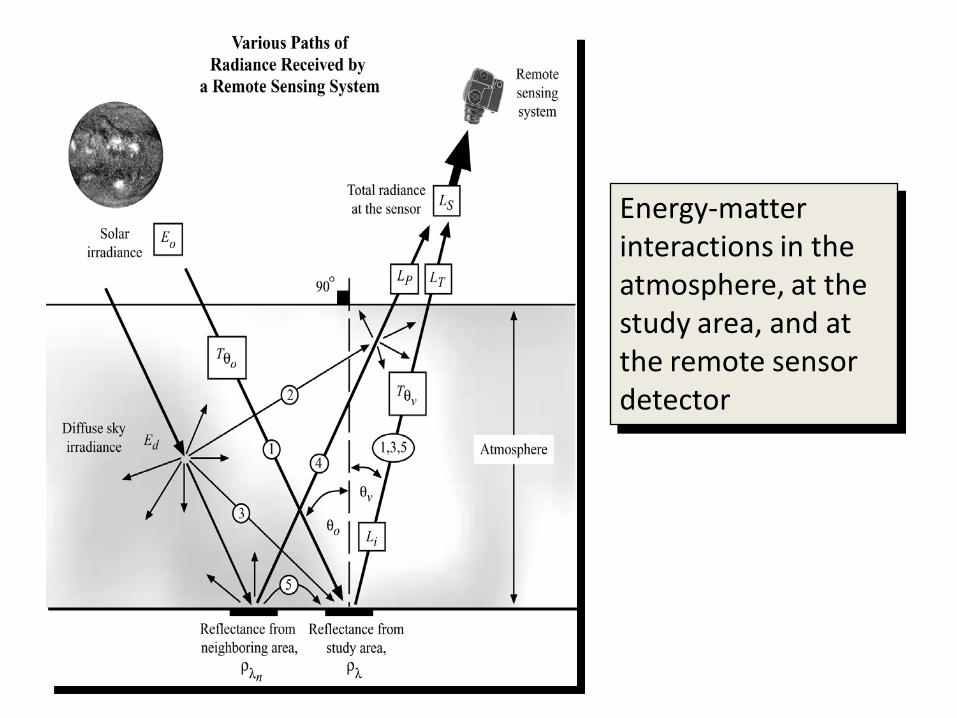
Energy-matter interactions in the atmosphere, at the study area, and at the remote sensor detector
Transcript of Energy-matter interactions in the atmosphere, at the...
Energy-matter interactions in the atmosphere, at the study area, and at the remote sensor detector
Scattering
Once electromagnetic radiation is generated, it is propagated through the earth's atmosphere almost at the speed of light in a vacuum.
• Unlike a vacuum in which nothing happens, however, the atmosphere may affect not only the speed of radiation but also its wavelength, intensity, spectral distribution, and/or direction.

Scatter differs from reflection in that the direction associated with scattering is unpredictable, whereas the direction of reflection is predictable. There are essentially three types of scattering:
• Rayleigh,
• Mie, and
• Non-selective.
Scattering

Major subdivisions of the atmosphere and the types of molecules and aerosols found in each layer.
Atmospheric Layers and Constituents

Rayleigh scattering occurs when the diameter of the matter (usually air molecules) are many times smaller than the wavelength of the incident electromagnetic radiation. This type of scattering is named after the English physicist who offered the first coherent explanation for it. All scattering is accomplished through absorption and re-emission of radiation by atoms or molecules in the manner described in the discussion on radiation from atomic structures. It is impossible to predict the direction in which a specific atom or molecule will emit a photon, hence scattering.
The energy required to excite an atom is associated with short-wavelength, high frequency radiation. The amount of scattering is inversely related to the fourth power of the radiation's wavelength. For example, blue light (0.4 µm) is scattered 16 times more than near-infrared light (0.8 µm).
Rayleigh Scattering

Atmospheric Scattering
Type of scattering is a function of:
• the wavelength of the incident radiant energy, and
• the size of the gas molecule, dust particle, and/or water vapor droplet encountered.

RayleighScattering
The intensity of Rayleigh scattering varies inversely with the fourth power of the wavelength (λ-
4).

Rayleigh Scattering
• Rayleigh scattering is responsible for the blue sky. The short violet and blue wavelengths are more efficiently scattered than the longer orange and red wavelengths. When we look up on cloudless day and admire the blue sky, we witness the preferential scattering of the short wavelength sunlight.
• Rayleigh scattering is responsible for red sunsets. Since the atmosphere is a thin shell of gravitationally bound gas surrounding the solid Earth, sunlight must pass through a longer slant path of air at sunset (or sunrise) than at noon. Since the violet and blue wavelengths are scattered even more during their now-longer path through the air than when the Sun is overhead, what we see when we look toward the Sun is the residue - the wavelengths of sunlight that are hardly scattered away at all, especially the oranges and reds (Sagan, 1994).

The approximate amount of Rayleigh scattering in the atmosphere in optical wavelengths (0.4 – 0.7 µm) may be computed using the Rayleigh scattering cross-section (τm) algorithm:
where n = refractive index, N = number of air molecules per unit volume, and λ = wavelength. The amount of scattering is inversely related to the fourth power of the radiation’s wavelength.
( )( )42
223
318
λπτ
Nn
m−
=
Rayleigh Scattering

Mie Scattering
• Mie scattering takes place when there are essentially spherical particles present in the atmosphere with diameters approximately equal to the wavelength of radiation being considered. For visible light, water vapor, dust, and other particles ranging from a few tenths of a micrometer to several micrometers in diameter are the main scattering agents. The amount of scatter is greater than Rayleigh scatter and the wavelengths scattered are longer.
• Pollution also contributes to beautiful sunsets and sunrises. The greater the amount of smoke and dust particles in the atmospheric column, the more violet and blue light will be scattered away and only the longer orange and red wavelength light will reach our eyes.

Non-selective Scattering
• Non-selective scattering is produced when there are particles in the atmosphere several times the diameter of the radiation being transmitted. This type of scattering is non-selective, i.e. all wavelengths of light are scattered, not just blue, green, or red. Thus, water droplets, which make up clouds and fog banks, scatter all wavelengths of visible light equally well, causing the cloud to appear white (a mixture of all colors of light in approximately equal quantities produces white).
• Scattering can severely reduce the information content of remotely sensed data to the point that the imagery looses contrast and it is difficult to differentiate one object from another.

• Absorption is the process by which radiant energy is absorbed and converted into other forms of energy. An absorption band is a range of wavelengths (or frequencies) in the electromagnetic spectrum within which radiant energy is absorbed by substances such as water (H2O), carbon dioxide (CO2), oxygen (O2), ozone (O3), and nitrous oxide (N2O).
• The cumulative effect of the absorption by the various constituents can cause the atmosphere to close down in certain regions of the spectrum. This is bad for remote sensing because no energy is available to be sensed.
Absorption
• In certain parts of the spectrum such as the visible region (0.4 - 0.7 µm), the atmosphere does not absorb all of the incident energy but transmits it effectively. Parts of the spectrum that transmit energy effectively are called “atmospheric windows”.
• Absorption occurs when energy of the same frequency as the resonant frequency of an atom or molecule is absorbed, producing an excited state. If, instead of re-radiating a photon of the same wavelength, the energy is transformed into heat motion and is reradiated at a longer wavelength, absorption occurs. When dealing with a medium like air, absorption and scattering are frequently combined into an extinction coefficient.
• Transmission is inversely related to the extinction coefficient times the thickness of the layer. Certain wavelengths of radiation are affected far more by absorption than by scattering. This is particularly true of infrared and wavelengths shorter than visible light.
Absorption
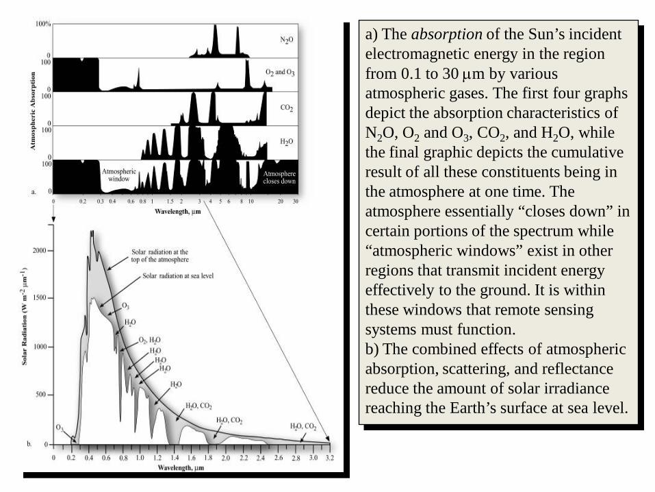
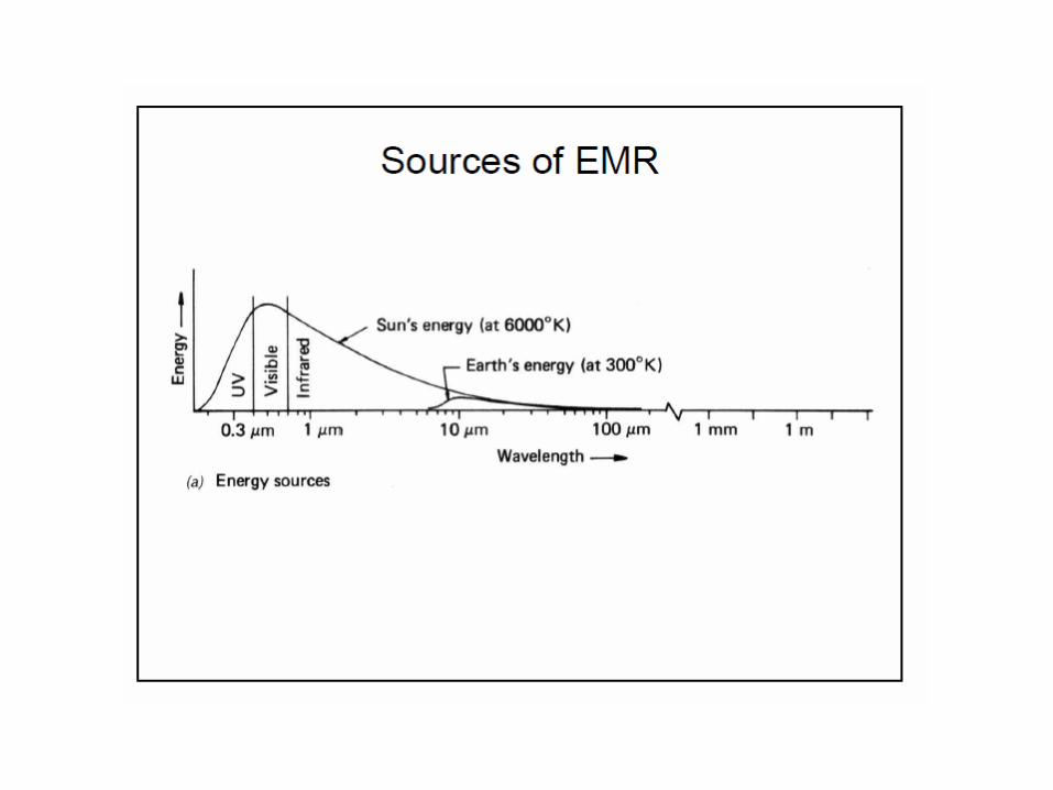
a) The absorption of the Sun’s incident electromagnetic energy in the region from 0.1 to 30 µm by various atmospheric gases. The first four graphs depict the absorption characteristics of N2O, O2 and O3, CO2, and H2O, while the final graphic depicts the cumulative result of all these constituents being in the atmosphere at one time. The atmosphere essentially “closes down” in certain portions of the spectrum while “atmospheric windows” exist in other regions that transmit incident energy effectively to the ground. It is within these windows that remote sensing systems must function. b) The combined effects of atmospheric absorption, scattering, and reflectance reduce the amount of solar irradiance reaching the Earth’s surface at sea level.

Reflectance is the process whereby radiation “bounces off” an object like a cloud or the terrain. Actually, the process is more complicated, involving re-radiation of photons in unison by atoms or molecules in a layer one-half wavelength deep.
• Reflection exhibits fundamental characteristics that are important in remote sensing. First, the incident radiation, the reflected radiation, and a vertical to the surface from which the angles of incidence and reflection are measured all lie in the same plane. Second, the angle of incidence and the angle of reflection are equal.
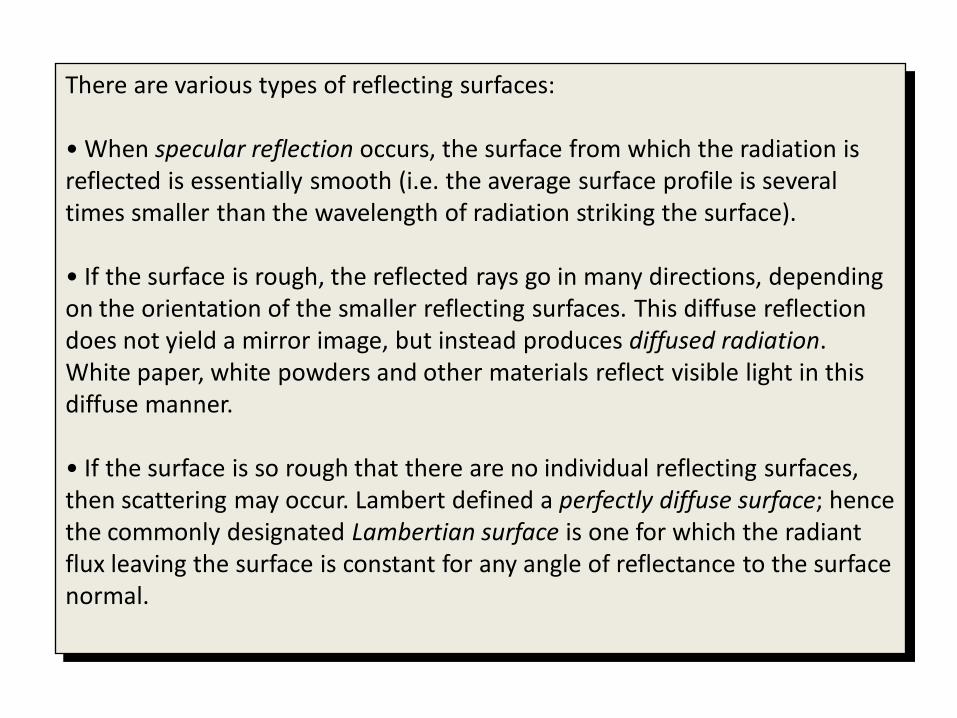
There are various types of reflecting surfaces:
• When specular reflection occurs, the surface from which the radiation is reflected is essentially smooth (i.e. the average surface profile is several times smaller than the wavelength of radiation striking the surface).
• If the surface is rough, the reflected rays go in many directions, depending on the orientation of the smaller reflecting surfaces. This diffuse reflection does not yield a mirror image, but instead produces diffused radiation. White paper, white powders and other materials reflect visible light in this diffuse manner.
• If the surface is so rough that there are no individual reflecting surfaces, then scattering may occur. Lambert defined a perfectly diffuse surface; hence the commonly designated Lambertian surface is one for which the radiant flux leaving the surface is constant for any angle of reflectance to the surface normal.

Reflectance

The concept of radiant flux densityfor an area on the surface of the Earth.
• Irradiance is a measure of the amount of radiant flux incident upon a surface per unit area of the surface measured in watts m-
2.
• Exitance is a measure of the amount of radiant flux leaving a surface per unit area of the surface measured in watts m-2.
Radiant Flux Density
Radiance
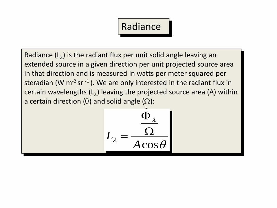
Radiance (Lλ) is the radiant flux per unit solid angle leaving an extended source in a given direction per unit projected source area in that direction and is measured in watts per meter squared per steradian (W m-2 sr -1 ). We are only interested in the radiant flux in certain wavelengths (Lλ) leaving the projected source area (A) within a certain direction (θ) and solid angle (Ω):
Φ Ω
Lλ = ______ Α cos θ
θ
λ
λ cosAL Ω
Φ
=
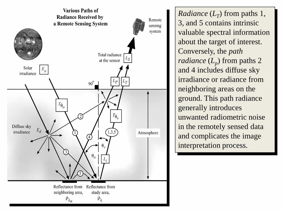
Radiance (LT) from paths 1, 3, and 5 contains intrinsic valuable spectral information about the target of interest. Conversely, the path radiance (Lp) from paths 2 and 4 includes diffuse sky irradiance or radiance from neighboring areas on the ground. This path radiance generally introduces unwanted radiometric noise in the remotely sensed data and complicates the image interpretation process.
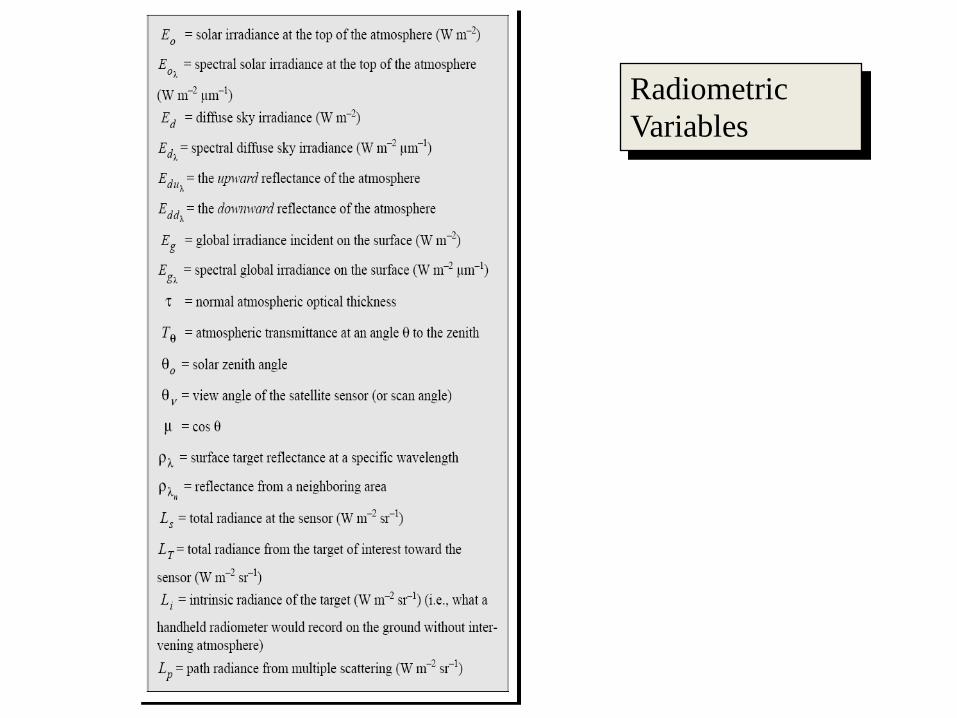
Radiometric Variables
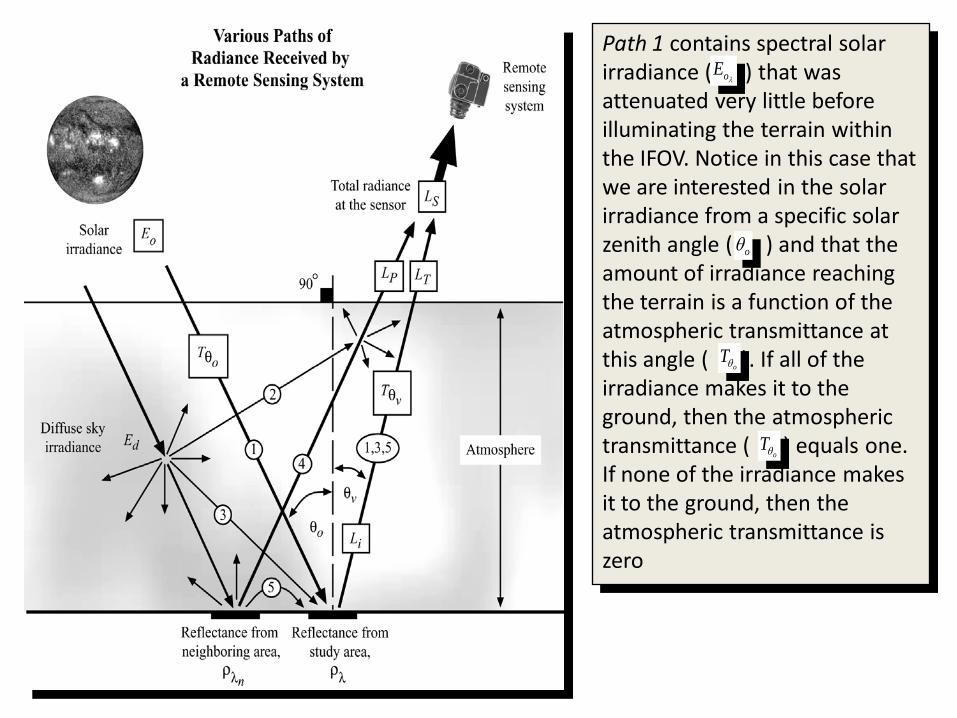
Path 1 contains spectral solar irradiance ( ) that was attenuated very little before illuminating the terrain within the IFOV. Notice in this case that we are interested in the solar irradiance from a specific solar zenith angle ( ) and that the amount of irradiance reaching the terrain is a function of the atmospheric transmittance at this angle ( ). If all of the irradiance makes it to the ground, then the atmospheric transmittance ( ) equals one. If none of the irradiance makes it to the ground, then the atmospheric transmittance is zero
λoE
oθ
oTθ
oTθ
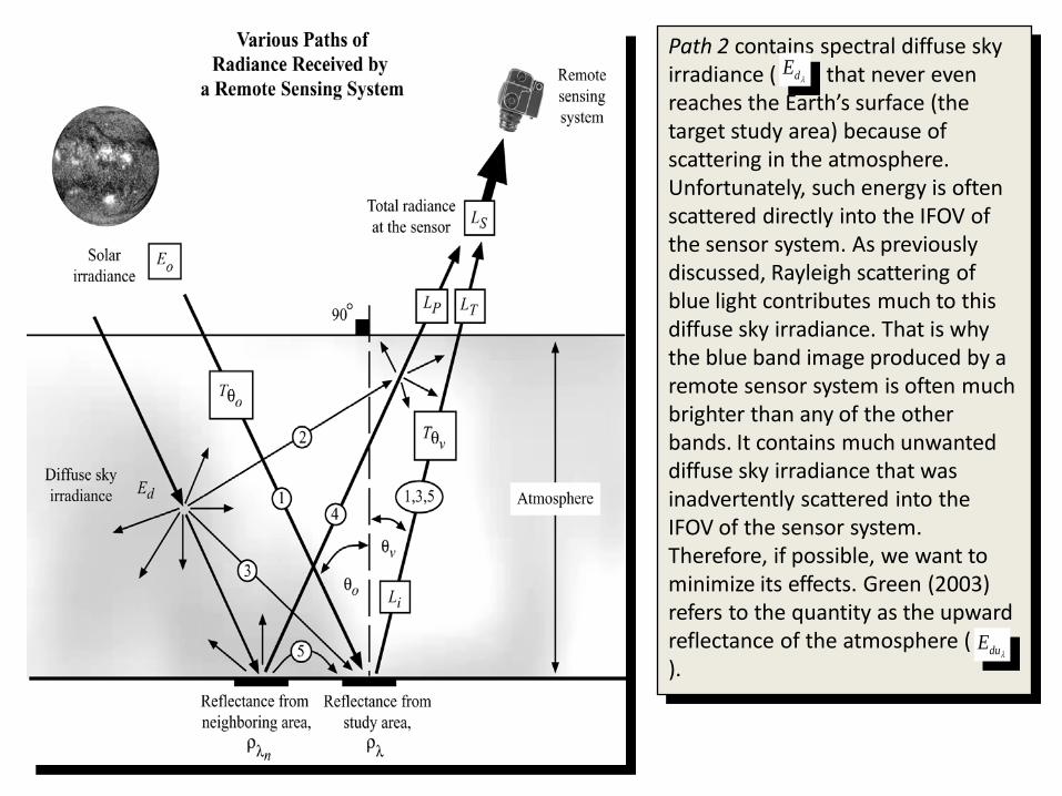
Path 2 contains spectral diffuse sky irradiance ( ) that never even reaches the Earth’s surface (the target study area) because of scattering in the atmosphere. Unfortunately, such energy is often scattered directly into the IFOV of the sensor system. As previously discussed, Rayleigh scattering of blue light contributes much to this diffuse sky irradiance. That is why the blue band image produced by a remote sensor system is often much brighter than any of the other bands. It contains much unwanted diffuse sky irradiance that was inadvertently scattered into the IFOV of the sensor system. Therefore, if possible, we want to minimize its effects. Green (2003) refers to the quantity as the upward reflectance of the atmosphere ( ).
λdE
λduE
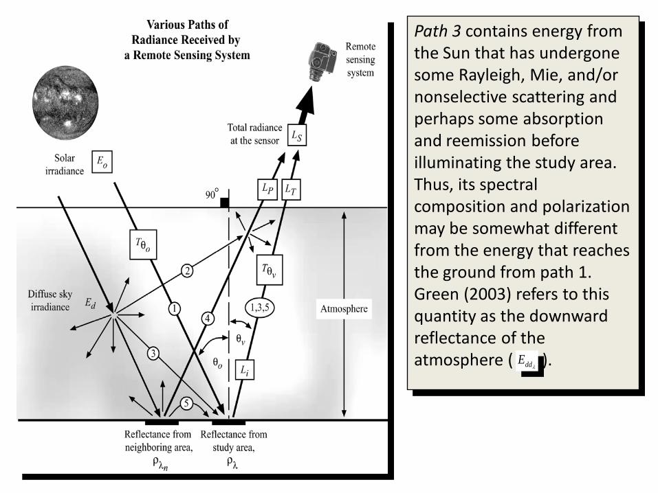
Path 3 contains energy from the Sun that has undergone some Rayleigh, Mie, and/or nonselective scattering and perhaps some absorption and reemission before illuminating the study area. Thus, its spectral composition and polarization may be somewhat different from the energy that reaches the ground from path 1. Green (2003) refers to this quantity as the downward reflectance of the atmosphere ( ).λddE
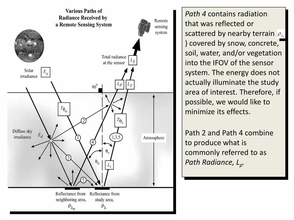
Path 4 contains radiation that was reflected or scattered by nearby terrain ( ) covered by snow, concrete, soil, water, and/or vegetation into the IFOV of the sensor system. The energy does not actually illuminate the study area of interest. Therefore, if possible, we would like to minimize its effects.
Path 2 and Path 4 combine to produce what is commonly referred to as Path Radiance, Lp.
nλρ

Path 5 is energy that was also reflected from nearby terrain into the atmosphere, but then scattered or reflected onto the study area.

The total radiance reaching the sensor from the target is:
pTS LLL +=
The total radiance recorded by the sensor becomes:
( ) λθρπ θλθ
λ
λλ dETETL dooovT += ∫ cos1 2
1
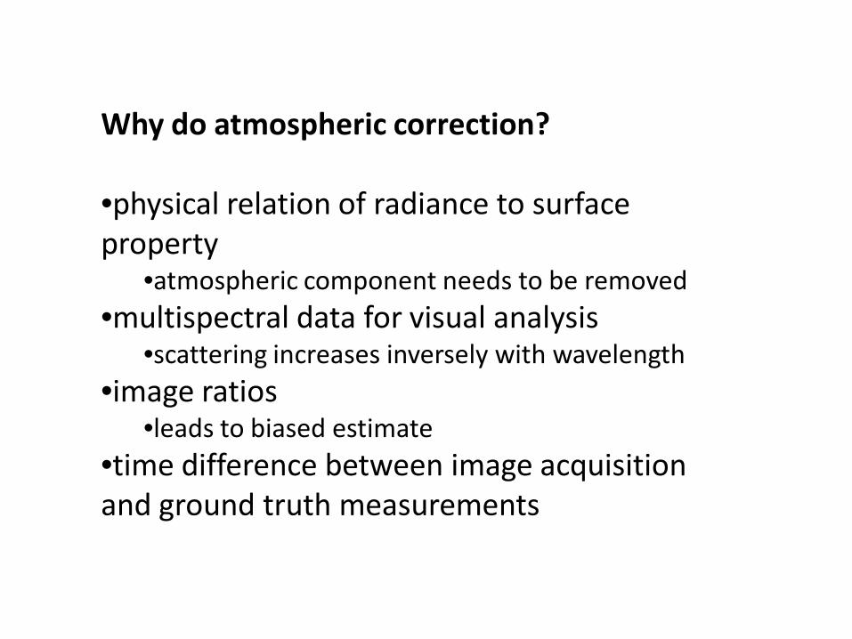
Why do atmospheric correction?
•physical relation of radiance to surfaceproperty
•atmospheric component needs to be removed•multispectral data for visual analysis
•scattering increases inversely with wavelength•image ratios
•leads to biased estimate•time difference between image acquisition and ground truth measurements


Atmospheric correction
• There are several ways to atmospherically correct remotely sensed data. Some are relatively straightforward while others are complex, being founded on physical principles and requiring a significant amount of information to function properly. This discussion will focus on two major types of atmospheric correction:
– Absolute atmospheric correction, and
– Relative atmospheric correction.
Solar irradiance
Reflectance from study area,
Various Paths of Satellite Received Radiance
Diffuse sky irradiance
Total radiance at the sensor
L L
L
Reflectance from neighboring area,
1
2
3
Remote sensor
detector
Atmosphere
5
4 1,3,5
θ
θ
E
L
90Þ
θ0T
θv T
0
0
v
p T
S
I
λ nr λ r
Ed
60 milesor100km
Scattering, AbsorptionRefraction, Reflection
Absolute atmospheric correction
• Solar radiation is largely unaffected as it travels through the vacuum of space. When it interacts with the Earth’s atmosphere, however, it is selectively scattered and absorbed. The sum of these two forms of energy loss is called atmospheric attenuation. Atmospheric attenuation may 1) make it difficult to relate hand-held in situ spectroradiometer measurements with remote measurements, 2) make it difficult to extend spectral signatures through space and time, and (3) have an impact on classification accuracy within a scene if atmospheric attenuation varies significantly throughout the image.
• The general goal of absolute radiometric correction is to turn the digital brightness values (or DN) recorded by a remote sensing system into scaled surface reflectance values. These values can then be compared or used in conjunction with scaled surface reflectance values obtained anywhere else on the planet.

Absolute Correction
Absolute radiometric correction takes into account measured atmospheric conditions (contributing to radiative transfer), as well as sensor gains and offsets, solar irradiance and solar zenith angle at the time of image acquisition, to calculate exoatmosphericreflectance values as they would have been measured on the ground.
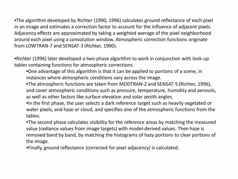
•The algorithm developed by Richter (1990, 1996) calculates ground reflectance of each pixel in an image and estimates a correction factor to account for the influence of adjacent pixels. Adjacency effects are approximated by taking a weighted average of the pixel neighborhood around each pixel using a convolution window. Atmospheric correction functions originate from LOWTRAN-7 and SENSAT-3 (Richter, 1990).
•Richter (1996) later developed a two-phase algorithm to work in conjunction with look-up tables containing functions for atmospheric corrections.
•One advantage of this algorithm is that it can be applied to portions of a scene, in instances where atmospheric conditions vary across the image. •The atmospheric functions are taken from MODTRAN-2 and SENSAT-5 (Richter, 1996), and cover atmospheric conditions such as pressure, temperature, humidity and aerosols, as well as other factors like surface elevation and solar zenith angles. •In the first phase, the user selects a dark reference target such as heavily vegetated or water pixels, and haze or cloud, and specifies one of the atmospheric functions from the tables. •The second phase calculates visibility for the reference areas by matching the measured value (radiance values from image targets) with model-derived values. Then haze is removed band by band, by matching the histograms of hazy portions to clear portions of the image. •Finally, ground reflectance (corrected for pixel adjacency) is calculated.


Atmospheric Correction Using ATCOR
a) Image containing substantial haze prior to atmospheric correction. b) Image after atmospheric correction using ATCOR (Courtesy Leica Geosystems and DLR, the German Aerospace Centre).
Absolute correction methods tend to be more accurate than relative corrections, or standardization methods, but have the disadvantage of being dependent on in situ data that may not be available.

Relative Correction
•An alternative to absolute radiometric correction is relative “correction,” which is commonly used in one of two ways: adjusting individual bands of data within a single image (i.e., based on subtracting dark object values from each band) or normalizing bands in images of multiple dates relative to a reference image (Jensen, 1996). •The primary difference to note between the two general approaches to relative normalization is that a master image is selected in studies involving multiple images of the same area.
relative radiometric correction
• When required data is not available for absolute radiometric correction, we can do relative radiometric correction
• Relative radiometric correction may be used to– Single-image normalization using histogram
adjustment– Multiple-data image normalization using
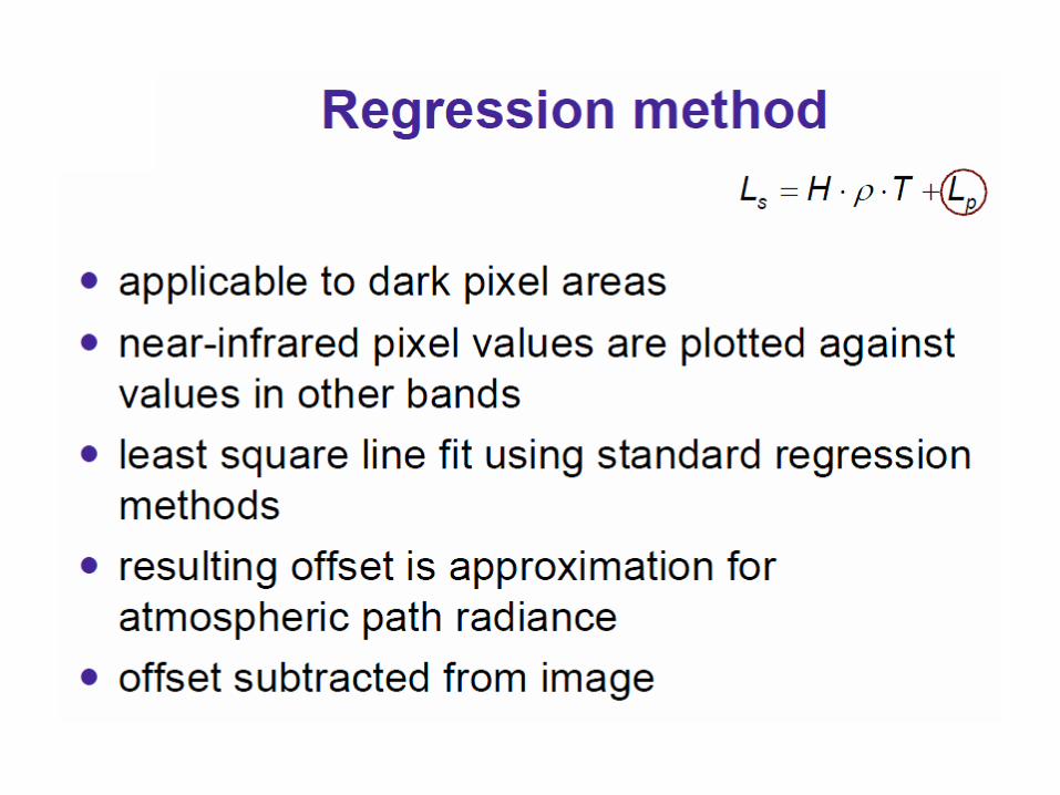
regression
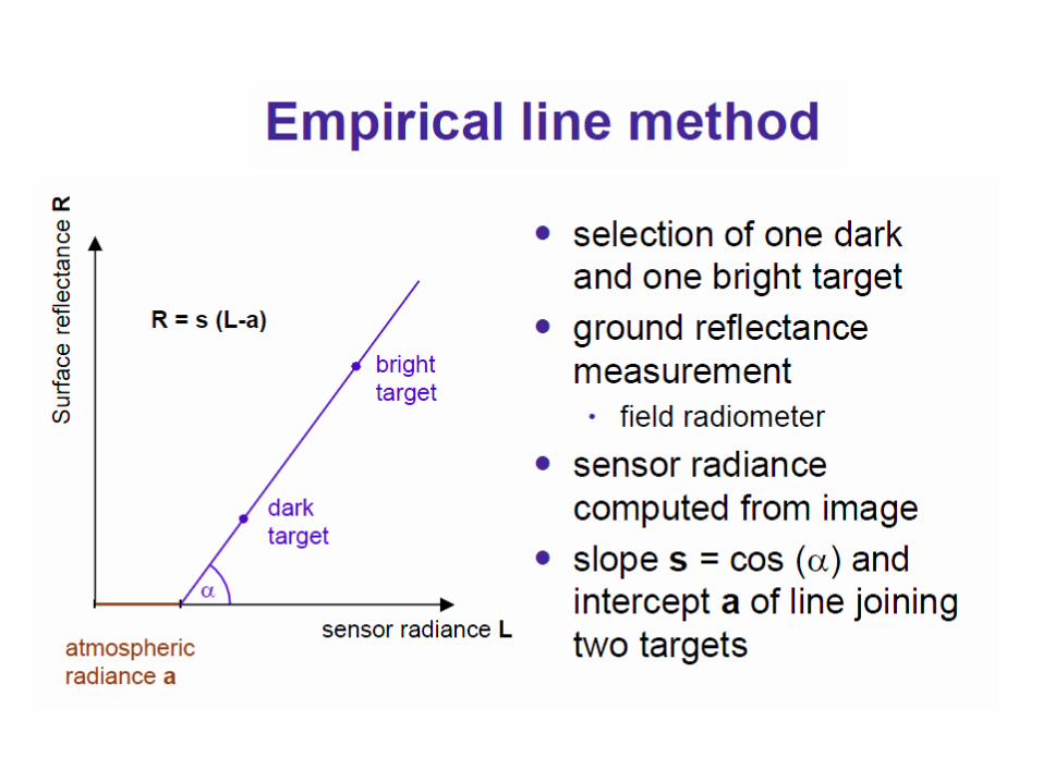
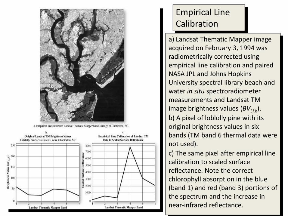
Empirical Line Calibration
a) Landsat Thematic Mapper image acquired on February 3, 1994 was radiometrically corrected using empirical line calibration and paired NASA JPL and Johns Hopkins University spectral library beach and water in situ spectroradiometer measurements and Landsat TM image brightness values (BVi,j,k). b) A pixel of loblolly pine with its original brightness values in six bands (TM band 6 thermal data were not used). c) The same pixel after empirical line calibration to scaled surface reflectance. Note the correct chlorophyll absorption in the blue (band 1) and red (band 3) portions of the spectrum and the increase in near-infrared reflectance.
Single-image normalization using histogram adjustment
• The method is based on the fact that infrared data (>0.7 µm) is free of atmospheric scattering effects, whereas the visible region (0.4-0.7 µm) is strongly influenced by them.
• Use Dark Subtract to apply atmospheric scattering corrections to the image data. The digital number to subtract from each band can be either the band minimum, an average based upon a user defined region of interest, or a specific value

Dark Subtract using band minimum
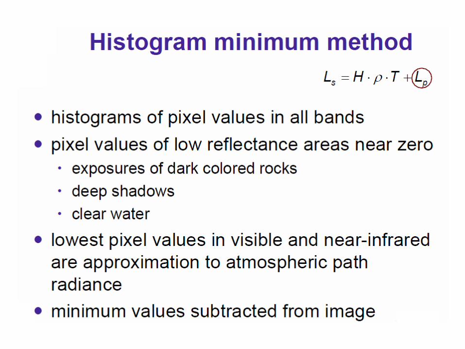
Single Image •Dark-object subtraction (DOS) is a widely used method of reducing haze within an image and is done for each band individually. •It is assumed that there are pixels within each band of a multispectral image that have very low or no reflectance on the ground, and that the difference between the brightness value of these pixels and zero is due to haze. This per-band estimated difference is subtracted from each band of the image (Chavez, 1988). •This relative normalization method assumes that the effects of haze are distributed evenly across the entire image, which may or may not be the case.•This is a good initial adjustment, but Chavez (1988) notes that there may be problems analyzing the data unless one of five atmospheric scattering models (scaled from very clear to very hazy) is chosen in addition to a dark-object haze value.

•Chavez (1996) further improved the technique of relative atmospheric standardization by adding a multiplicative correction factor for the effect of atmospheric transmittance. This approach is called the COST method named after the cosine of the solar zenith angle (Cos 2). •He compares this method to one that uses in situ field measurements of the atmosphere and finds that the image-based adjustments are as accurate as absolute correction algorithms that require additional information. This assessment is not made statistically but graphically, using scatter plots and bar charts to illustrate differences in the performance of different atmospheric correction algorithms.

Multiple Image •Due to the number of images that may be involved in a multitemporal change detection study and the scarcity of historical atmospheric and ground reflectance data, researchers often opt for a normalization method that corrects a set of images relative to a reference image.
•One multiple image method is based on identification of pseudoinvariant features, or features that are assumed to have the same spectral reflectance through the series of images (Jensen, 1996). The ideal pseudoinvariant targets are those that meet the following criteria: 1. Are at approximately the same elevation as the rest of the scene (for a better representation of the atmospheric conditions across the scene), 2. Are in a relatively flat area (to minimize the effects of solar azimuth differences) 3. Should have a minimal amount of vegetation (as vegetation readily changes in response to seasonal changes and environmental stresses) .

•In this method, statistical adjustments are based on the assumption that the differences in gray-level distributions of invariant objects are assumed to be a linear function. •Pseudoinvariant targets tend to be urban features (roads, buildings) because they are assumed to change little through time. These features are selected by identifying pixels that are dark in an infrared-red ratio (TM 4/3) image and bright in the mid-infrared (TM band 7). •After normalization targets are chosen, the target brightness values from the scenes to be normalized are regressed against the target brightness of the reference image. •This is a linear regression model relating each band of each pairing of images, consisting of an additive component (intercept) which accounts for the difference in path radiance, and a multiplicative component (slope) which corrects for differences in detector calibration, sun angle, Earth-sun distance, atmospheric influences and sun-target-sensor geometry between dates.

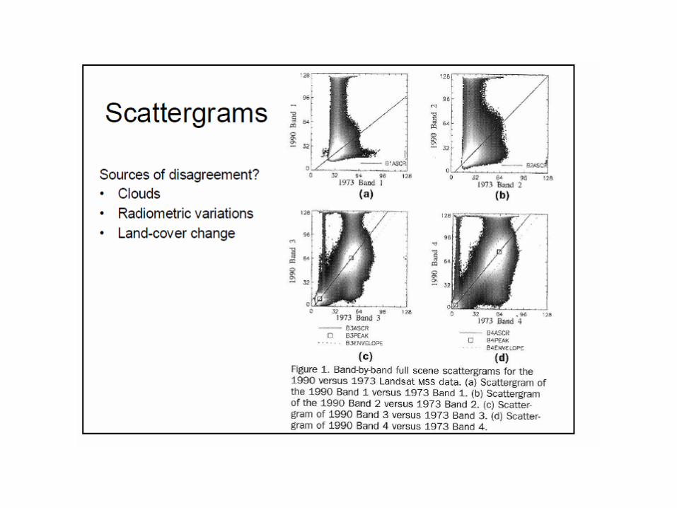
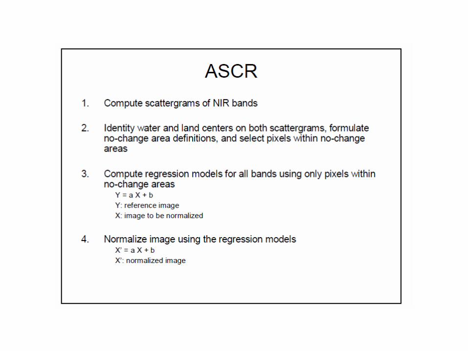
•Another technique is an automatic scattergram-controlled regression (ASCR) method, developed by Elvidge et al. (1995) for use with large sets of Landsat images.• This method uses scattergrams of the near-infrared bands of image date 1 and date 2 to identify stable land and water data clusters and generate an initial regression line between the two cluster centers.• A no-change pixel set is selected by placing thresholds about this line. These pixels are then used in the regression analysis of each band to derive gains and offsets for the radiometric normalization. Requirements for this method are that:
1. Images are acquired under similar solar and phenological conditions. 2. Land cover for a large portion of the image in the time covered by the images to be rectified has not changed. 3. There are both land and water pixels in the scene.

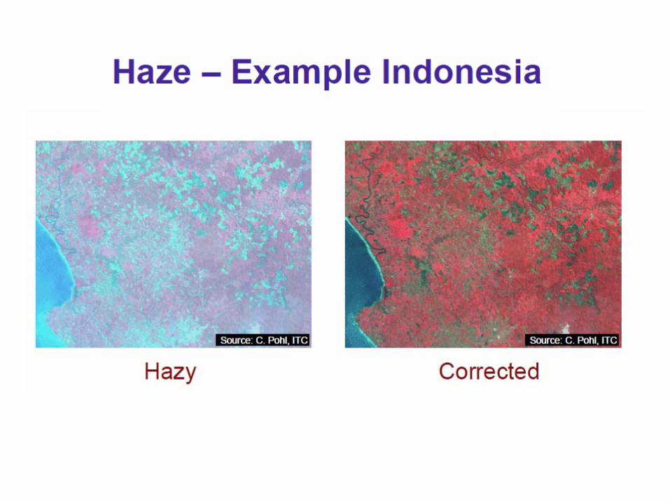
•This method is shown to significantly reduce haze, making images more comparable spectrally. The researchers also list advantages of this procedure over other linear relative normalization methods: 1. Cloud/shadow/snow effects are reduced compared with simple regression methods. 2. A large percentage of the total number of image pixels is used. 3. Normalization errors are distributed among different land cover types. 4. The necessity of identifying bright and dark radiometric control pixels is eliminated. 5. The speed of the normalization procedure is accelerated by reducing human intervention (though it may not reduce the computation time).


Topographic correction
• Topographic slope and aspect also introduce radiometric distortion (for example, areas in shadow)
• The goal of a slope-aspect correction is to remove topographically induced illumination variation so that two objects having the same reflectance properties show the same brightness value (or DN) in the image despite their different orientation to the Sun’s position
• Based on DEM, sun-elevation
Accuracy Assessment
Goals: – Assess how well a
classification worked– Understand how to interpret
the usefulness of someone else’s classification

Accuracy Assessment
• Overview– Collect reference data: “ground
truth”• Determination of class types at specific
locations
– Compare reference to classified map• Does class type on classified map = class
type determined from reference data?

Accuracy Assessment: Reference Data
• Some possible sources– Aerial photo
interpretation– Ground truth with GPS– GIS layers

Accuracy Assessment: Reference Data
• Issue 1: Choosing reference source– Make sure you can actually extract from the
reference source the information that you need for the classification scheme
• I.e. Aerial photos may not be good reference data if your classification scheme distinguishes four species of grass. You may need GPS’d ground data.

Accuracy Assessment: Reference data
• Issue 2: Determining size of reference plots– Match spatial scale of reference plots and
remotely-sensed data• I.e. GPS’d ground plots 5 meters on a side may not be
useful if remotely-sensed cells are 1km on a side. You may need aerial photos or even other satellite images.
Accuracy Assessment: Reference Data
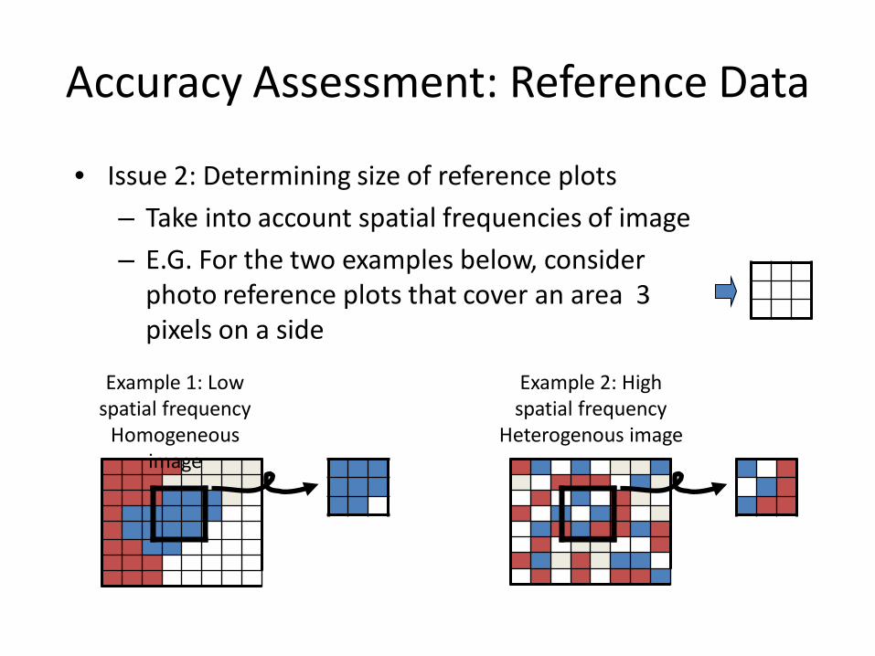
• Issue 2: Determining size of reference plots– Take into account spatial frequencies of image– E.G. For the two examples below, consider
photo reference plots that cover an area 3 pixels on a side
Example 1: Low spatial frequency
Homogeneous image
Example 2: High spatial frequency
Heterogenous image

Accuracy Assessment: Reference Data
• Issue 2: Determining size of reference plots– HOWEVER, also need to take into account accuracy
of position of image and reference data– E.G. For the same two examples, consider the
situation where accuracy of position of the image is +/- one pixel
Example 1: Low spatial frequency
Example 2: High spatial frequency

Accuracy Assessment: Reference Data
• Issue 3: Determining position and number of samples– Make sure to adequately sample the landscape– Variety of sampling schemes
• Random, stratified random, systematic, etc.– The more reference plots, the better
• You can estimate how many you need statistically• In reality, you can never get enough• Lillesand and Kiefer: suggest 50 per class as rule of
thumb

Sampling Methods
Simple Random Sampling :
observations are randomly placed.
Stratified Random Sampling : aminimum number of observationsare randomly placed in eachcategory.

Sampling Methods
Systematic Sampling : observationsare placed at equal intervalsaccording to a strategy.
Systematic Non-Aligned Sampling:a grid provides even distribution ofrandomly placed observations.

Sampling Methods
Cluster Sampling : Randomlyplaced “centroids” used as a baseof several nearby observations. The nearby observations can berandomly selected, systematicallyselected, etc...

Accuracy Assessment: Reference data
• Having chosen reference source, plot size, and locations:– Determine class types from reference source– Determine class type claimed by classified map
• Compare them!
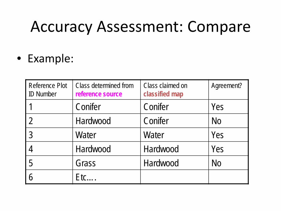
Accuracy Assessment: Compare
• Example:
Reference Plot ID Number
Class determined from reference source
Class claimed on classified map
Agreement?
1 Conifer Conifer Yes2 Hardwood Conifer No3 Water Water Yes4 Hardwood Hardwood Yes5 Grass Hardwood No6 Etc….
Accuracy Assessment: Compare
How to summarize and quantify?
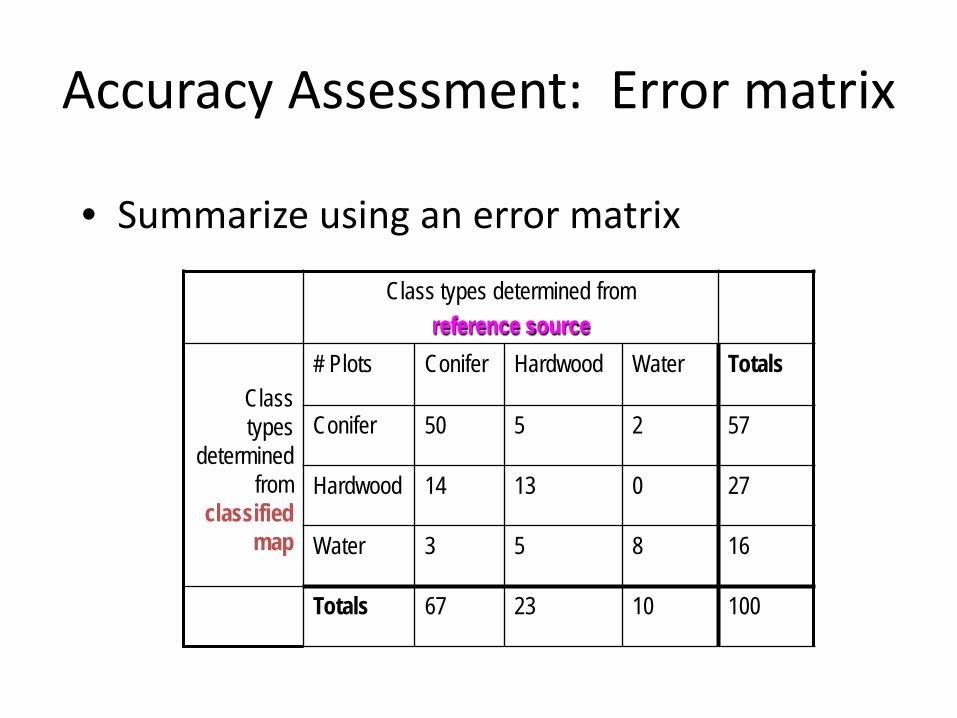
Accuracy Assessment: Error matrix
• Summarize using an error matrix
Class types determined from reference source
Class types
determined from
classified map
# Plots Conifer Hardwood Water Totals
Conifer 50 5 2 57
Hardwood 14 13 0 27
Water 3 5 8 16
Totals 67 23 10 100
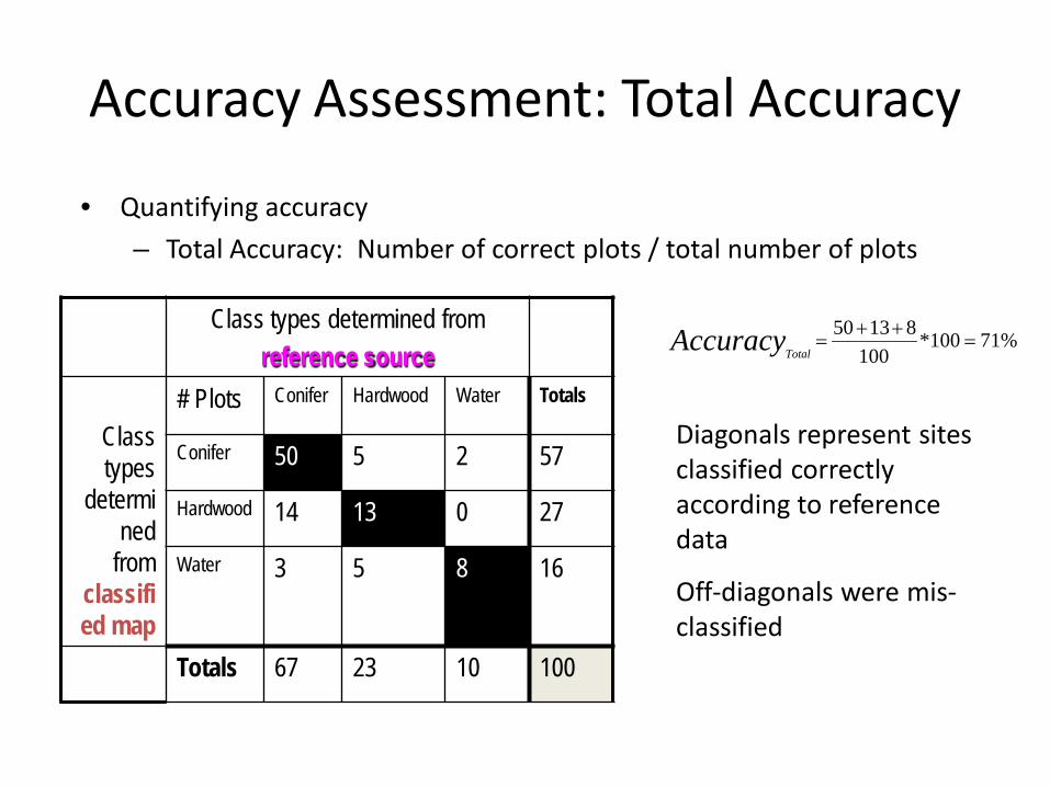
Accuracy Assessment: Total Accuracy
• Quantifying accuracy– Total Accuracy: Number of correct plots / total number of plots
Class types determined from reference source
Class types
determined
from classified map
# Plots Conifer Hardwood Water Totals
Conifer 50 5 2 57
Hardwood 14 13 0 27
Water 3 5 8 16
Totals 67 23 10 100
%71100*100
81350=
++=AccuracyTotal
Diagonals represent sites classified correctly according to reference data
Off-diagonals were mis-classified

Accuracy Assessment: Total Accuracy
• Problem with total accuracy:– Summary value is an average
• Does not reveal if error was evenly distributed between classes or if some classes were really bad and some really good
• Therefore, include other forms:– User’s accuracy– Producer’s accuracy

User’s and producer’s accuracy and types of error
• User’s accuracy corresponds to error of commission (inclusion):– f.ex. 1 shrub and 3 conifer sites included
erroneously in grass category
• Producer’s accuracy corresponds to error of omission (exclusion):– f.ex. 7 conifer and 1 shrub sites omitted from grass
category

Accuracy Assessment: User’s Accuracy
• From the perspective of the user of the classified map, how accurate is the map?– For a given class, how many of the pixels on the
map are actually what they say they are?– Calculated as: Number correctly identified in a given map class /
Number claimed to be in that map class

Accuracy Assessment: User’s Accuracy
Class types determined from reference source
Class types
determined
from classified map
# Plots Conifer Hardwood Water Totals
Conifer 50 5 2 57
Hardwood 14 13 0 27
Water 3 5 8 16
Totals 67 23 10 100
%88100*5750
,'==Accuracy ConifersUser
Example: Conifer

Accuracy Assessment: Producer’s Accuracy
• From the perspective of the maker of the classified map, how accurate is the map?– For a given class in reference plots, how many of
the pixels on the map are labeled correctly?– Calculated as: Number correctly identified in ref. plots of a given
class / Number actually in that reference class

Accuracy Assessment: Producer’s Accuracy
Class types determined from reference source
Class types
determined
from classified map
# Plots Conifer Hardwood Water Totals
Conifer 50 5 2 57
Hardwood 14 13 0 27
Water 3 5 8 16
Totals 67 23 10 100
%75100*6750
==Accuracy Coniferproducers,
Example: Conifer

Accuracy Assessment: Summary so far
Class types determined from reference source
User’s AccuracyClass types
determined from
classified map
# Plots Conifer Hardwood Water Totals
Conifer 50 5 2 57 88%
Hardwood 14 13 0 27 48%
Water 3 5 8 16 50%
Totals 67 23 10 100
Producer’s Accuracy 75% 57% 80% Total: 71%

Accuracy Assessment: Kappa
• Kappa statistic• Estimated as • Reflects the difference between actual agreement and the
agreement expected by chance• Kappa of 0.85 means there is 85% better agreement than
by chance alone
K
agreement chance - 1agreement chance -accuracy observedˆ =K

Accuracy Assessment: Kappa
• Observed accuracy determined by diagonal in error matrix
• Chance agreement incorporates off-diagonal– Sum of [Product of row and column totals for each
class]– See Chapter 7 (p. 574) in Lillesand and Kiefer for
computational formula
agreement chance - 1agreement chance -accuracy observedˆ =K
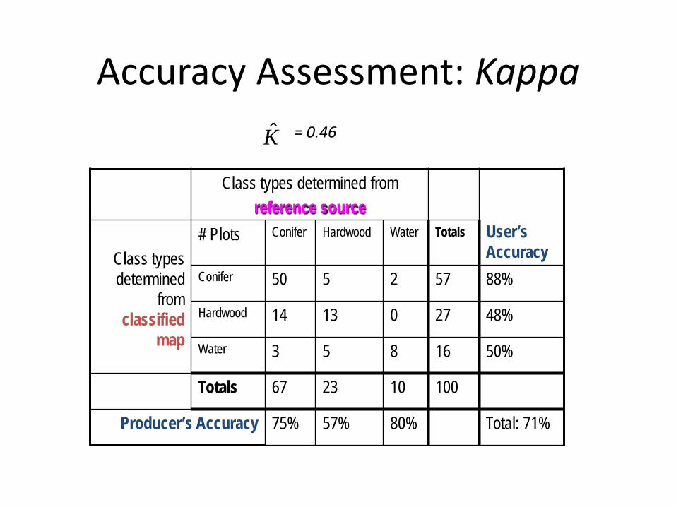
Accuracy Assessment: Kappa
Class types determined from reference source
User’s AccuracyClass types
determined from
classified map
# Plots Conifer Hardwood Water Totals
Conifer 50 5 2 57 88%
Hardwood 14 13 0 27 48%
Water 3 5 8 16 50%
Totals 67 23 10 100
Producer’s Accuracy 75% 57% 80% Total: 71%
= 0.46K

• Other uses of kappa– Compare two error matrices– Weight cells in error matrix according to severity of
misclassification– Provide error bounds on accuracy
Accuracy Assessment: Kappa

Accuracy Assessment: Quantifying
• Each type of accuracy estimate yields different information
• If we only focus on one, we may get an erroneous sense of accuracy

Accuracy Assessment: Quantifying• Example: Total accuracy was 71%, but User’s accuracy for
hardwoods was only 48%
Class types determined from reference source
User’s AccuracyClass types
determined from
classified map
# Plots Conifer Hardwood Water Totals
Conifer 50 5 2 57 88%
Hardwood 14 13 0 27 48%
Water 3 5 8 16 50%
Totals 67 23 10 100
Producer’s Accuracy 75% 57% 80% Total: 71%
Accuracy Assessment: Quantifying
• What to report?– Depends on audience– Depends on the objective of your study– Most references suggest full reporting of error
matrix, user’s and producer’s accuracies, total accuracy, and Kappa
Accuracy Assessment: Interpreting
• Why might accuracy be low?– Errors in reference data– Errors in classified map

Accuracy Assessment: Interpreting
• Errors in reference data– Positional error
• Better rectification of image may help
– Interpreter error– Reference medium inappropriate for classification

Accuracy Assessment: Interpreting
• Errors in classified map– Remotely-sensed data cannot capture classes
• Classes are land use, not land cover• Classes not spectrally separable• Atmospheric effects mask subtle differences• Spatial scale of remote sensing instrument does not
match classification scheme
Accuracy Assessment: Improving Classification
• Ways to deal with these problems:– Land use/land cover: incorporate other data
• Elevation, temperature, ownership, distance from streams, etc.
• Context– Spectral inseparability: add spectral data
• Hyperspectral• Multiple dates
– Atmospheric effects: Atmospheric correction mayhelp
– Scale: Change grain of spectral data• Different sensor• Aggregate pixels

Accuracy Assessment: Improving Classification
• Errors in classified map– Remotely-sensed data should be able to capture
classes, but classification strategy does not draw this out
• Minority classes swamped by larger trends in variability– Use HIERARCHICAL CLASSIFICATION scheme– In Maximum Likelihood classification, use Prior Probabilities to weigh
minority classes more

Accuracy Assessment: Summary
• Choice of reference data important– Consider interaction between sensor and desired
classification scheme• Error matrix is foundation of accuracy
assessment• All forms of accuracy assessment should be
reported to user• Interpreting accuracy in classes can yield ideas
for improvement of classification