Energy Management Strategies for Plug-in Hybrid Electric ...

Energy Management Strategies for Plug-in

Hybrid Electric Vehicles

Master of Science Thesis

Henrik Friden

Hanna Sahlin

Department of Signals and SystemsDivision of Automatic Control, Automation and MechatronicsCHALMERS UNIVERSITY OF TECHNOLOGYGoteborg, Sweden 2012Report No. EX043/2012

THESIS FOR THE DEGREE OF MASTER IN SCIENCE

Energy Management Strategies for Plug-in

Hybrid Electric Vehicles

Henrik FridenHanna Sahlin

Department of Signals and SystemsCHALMERS UNIVERSITY OF TECHNOLOGY

Goteborg, Sweden 2012

Energy Management Strategies for Plug-in Hybrid Electric Vehicles

Henrik FridenHanna Sahlin

cHenrik Friden, Hanna Sahlin, 2012

Master of Science Thesis in cooperation with Volvo Car CorporationReport No. EX043/2012Department of Signals and SystemsChalmers University of TechnologySE-412 96 GoteborgSwedenTelephone: + 46 (0)31-772 1000

Cover:Energy Management Strategies for Plug-in Hybrid Electric Vehicles

Chalmers ReproserviceGoteborg, Sweden 2012

Energy Management Strategies for Plug-in Hybrid Electric VehiclesHenrik Friden and Hanna SahlinDepartment of Signals and SystemsChalmers University of Technology

Abstract

Along with the common goal of reducing fuel consumption for vehicles, the hybridelectric vehicle stands out as a mean for more fuel efficient driving. Besides theconventional combustion engine and fuel tank, the hybrid electric vehicle is alsoequipped with an electric motor and a battery for propulsion. Car manufacturersare presently working to provide the markets with the next step of this concept,the plug-in hybrid electric vehicle, allowing the on-board battery to be rechargedfrom the power grid.

The aim of this master thesis is to evaluate two different energy managementstrategies for plug-in hybrid electric vehicles. These energy management strategiesconsist of both control strategies as well as battery discharge strategies.

This thesis evaluates an already existing control strategy based on rules forenergy management. It also involves Matlab R and Simulink R implementationof a control strategy; the Equivalent Consumption Minimization Strategy (ECMS),which is based on the concept of optimal control. ECMS operates by continuousevaluation of the fuel consumption cost for different power splits as a basis forselecting the most fuel efficient operating point between the internal combustionengine and the electric motor.

Two battery discharge strategies have been investigated. The first one is theCharge Depletion Charge Sustaining (CDCS) strategy, depleting the battery in anall-electric drive first and then operating in sustaining mode. The other method isto blend the use of the electric motor with the combustion engine at various pointsthroughout the entire trip in a blended mode discharge strategy.

A comparison has been made between a rule-based control strategy with CDCSand the ECMS control strategy for both blended and CDCS discharge. The com-parison is done with respect to fuel consumption but side effects related to thebattery power usage are observed as well. It is concluded that fuel consumptionusing ECMS with a blended discharge can be reduced by 4.2 % on average and by1.0 % on average for CDCS discharge, compared to using the rule-based controlstrategy with CDCS. Battery power losses are reduced by 15.6 % under a blendeddischarge strategy and by 7.9 % for CDCS discharge.

Keywords: Plug-in hybrid electric vehicle, ECMS, Optimal control, Charge Deple-tion Charge Sustaining, Blended discharge, Discharge strategies, Control strate-gies, Energy Management, Fuel consumption minimization.

, Signals and Systems, Master of Science Thesis 2012:06 i

Preface

This master thesis project was carried out during the spring of 2012 at Volvo CarCorporation, department of Complete powertrain located in Goteborg, Swedenand at Chalmers University of Technology, department of Signals and Systems,division of Automatic Control, Automation and Mechatronics.

We would like to thank our supervisor Anders Lasson at Volvo Car Coopera-tion for the support and valuable insight throughout this thesis project. Secondly,great thanks goes to our supervisor Viktor Larsson at Chalmers University ofTechnology, for guidance and quality discussions. We would also like to extendour thanks to our examiner Professor Bo Egardt for the questions and experienceyou have shared with us during the project.

Henrik and HannaGoteborg, June 2012

, Signals and Systems, Master of Science Thesis 2012:06 ii

AbbreviationsAER All Electric RangeCDCS Charge Depletion Charge SustainingECMS Equivalent Consumption Minimization StrategyECU Electric Control UnitEM Electric MotorEMS Energy Management SystemGB GearboxICE Internal Combustion EngineISG Integrated Starter GeneratorHEV Hybrid Electric VehicleNEDC New European Drive CyclePHEV Plug-in Hybrid Electric VehicleRMS Root Mean SquareSoC State of Charge

Physical parameters

Notations of the physical parameters with their unitsρair Density of air, [kg/m3]ηgr,EM Efficiency of the gear between the electrical motor and the rear wheelsηgr,belt Efficiency of the belt connection between the ICE and the ISGAf Front area, [m2]Cd Air dynamic drag resistanceDtot Estimated trip distance, [m]fr Rolling resistance coefficientg Acceleration of gravity, [m/s2]grEM Gear ratio between the electric motor and the rear wheelsgrbelt Gear ratio of the belt connection between the ICE and the ISGm Vehicle mass, [kg]Paux Auxiliary power, [W ]rwhl Wheel radius, [m]Q Electric charge capacity, [C]Qlhv Lower heating value, [J/kg]SoCfinal Final State of Charge, [%]SoCinit Initial State of Charge, [%]

, Signals and Systems, Master of Science Thesis 2012:06 iii

Physical variables

Notations of the physical variables with their unitsωwhl Wheel angular velocity, [rad/s]ωEM EM angular velocity, [rad/s]ωCrSh Crankshaft angular velocity, [rad/s]ωISG ISG angular velocity, [rad/s]θ Road grade, [rad]d Currently traveled distance, [m]Fdrive Drive force of the vehicle, [N ]Fdrag Drag force of the vehicle, [N ]Froll Rolling resistance force of the vehicle, [N ]Fgrade Road grade force of the vehicle, [N ]grGB Gearbox ratio between crankshaft and front wheelsi Battery current, [A]mfuel Fuel mass flow, [kg/s]Rbatt Battery resistance, [Ω]Pbatt Battery power, [W ]Pbatt,loss Battery losses, [W ]PEM,El Total EM power, [W ]PEM,mech Mechanical EM power, [W ]Pfuel,ICE ICE fuel power, [W ]Pfuel Total fuel power, [W ]PISG,El ISG total power [W ]Ploss,El Electrical power losses, [W ]Ploss,mech EM mechanical power losses, [W ]SoCref State of Charge reference, [%]SoC Current State of Charge, [%]TEM,whl EM torque seen at the wheels, [Nm]TEM EM torque seen at the motor, [Nm]TCrSh,whl Crankshaft torque seen at the wheels, [Nm]TCrSh Crankshaft torque, [Nm]TICE ICE torque seen at the engine, [Nm]TISG ISG torque seen at the shaft, [Nm]Twhl Requested torque at the wheels, [Nm]Vbatt Battery voltage, [V ]v Velocity, [m/s]

, Signals and Systems, Master of Science Thesis 2012:06 iv

Contents

Abstract i

Preface ii

Abbreviation iii

Physical parameters iii

Physical variables iii

Contents v

1 Introduction 1

1.1 Project background . . . . . . . . . . . . . . . . . . . . . . . . . . . 11.2 Aim . . . . . . . . . . . . . . . . . . . . . . . . . . . . . . . . . . . 21.3 Exclusions . . . . . . . . . . . . . . . . . . . . . . . . . . . . . . . . 31.4 Objectives . . . . . . . . . . . . . . . . . . . . . . . . . . . . . . . . 31.5 Outline . . . . . . . . . . . . . . . . . . . . . . . . . . . . . . . . . 3

2 The Hybrid Electric Vehicle 5

2.1 Powertrain configurations . . . . . . . . . . . . . . . . . . . . . . . 62.2 Investigated powertrain configuration . . . . . . . . . . . . . . . . . 8

3 Vehicle model 11

3.1 Dynamic powertrain model . . . . . . . . . . . . . . . . . . . . . . 113.2 Simplified powertrain model . . . . . . . . . . . . . . . . . . . . . . 13

3.2.1 Drive system power flows . . . . . . . . . . . . . . . . . . . 153.2.2 Power split ratio . . . . . . . . . . . . . . . . . . . . . . . . 17

3.3 Battery model . . . . . . . . . . . . . . . . . . . . . . . . . . . . . 18

4 The energy management problem 21

4.1 Rule-based control strategy . . . . . . . . . . . . . . . . . . . . . . 214.2 Discharge strategies . . . . . . . . . . . . . . . . . . . . . . . . . . 214.3 Optimal control . . . . . . . . . . . . . . . . . . . . . . . . . . . . . 234.4 Equivalent Consumption Minimization Strategy . . . . . . . . . . . 23

5 Implementation of ECMS 27

5.1 Stating the cost function . . . . . . . . . . . . . . . . . . . . . . . . 275.2 Engine startup cost . . . . . . . . . . . . . . . . . . . . . . . . . . . 285.3 Determining the equivalence factor . . . . . . . . . . . . . . . . . . 295.4 Implementing the ECMS algorithm . . . . . . . . . . . . . . . . . . 34

, Signals and Systems, Master of Science Thesis 2012:06 v

6 Results 37

6.1 Equivalence factor . . . . . . . . . . . . . . . . . . . . . . . . . . . 376.2 Start penalty . . . . . . . . . . . . . . . . . . . . . . . . . . . . . . 386.3 ECMS performance . . . . . . . . . . . . . . . . . . . . . . . . . . . 40

7 Analysis 49

7.1 Fuel consumption . . . . . . . . . . . . . . . . . . . . . . . . . . . . 497.2 Engine start cost . . . . . . . . . . . . . . . . . . . . . . . . . . . . 497.3 Battery operation . . . . . . . . . . . . . . . . . . . . . . . . . . . . 507.4 Drive cycle influence . . . . . . . . . . . . . . . . . . . . . . . . . . 507.5 Equivalence factor . . . . . . . . . . . . . . . . . . . . . . . . . . . 51

8 Discussion 53

8.1 Reducing the fuel consumption . . . . . . . . . . . . . . . . . . . . 538.2 Battery life . . . . . . . . . . . . . . . . . . . . . . . . . . . . . . . 538.3 Modeling errors . . . . . . . . . . . . . . . . . . . . . . . . . . . . . 548.4 Estimation of equivalence factor . . . . . . . . . . . . . . . . . . . . 558.5 Estimation errors . . . . . . . . . . . . . . . . . . . . . . . . . . . . 55

9 Future work 57

9.1 Better engine start cost . . . . . . . . . . . . . . . . . . . . . . . . 579.2 Mechanical energy reference . . . . . . . . . . . . . . . . . . . . . . 579.3 Route recognition . . . . . . . . . . . . . . . . . . . . . . . . . . . . 579.4 ECMS model update . . . . . . . . . . . . . . . . . . . . . . . . . . 589.5 ECU implementation . . . . . . . . . . . . . . . . . . . . . . . . . . 58

10 Conclusions 59

References 61

Appendices I

A Drive cycles I

B List of inputs and constants to the ECMS algorithm V

C The variation of s(t) VII

, Signals and Systems, Master of Science Thesis 2012:06 vi

1 Introduction

In times of frequent debate regarding the price, peak production, politics andsecure delivery of oil as well as if or how to best prevent climate change, themuch oil associated automotive industry is consequently handed a list of mattersto consider. One way of decreasing the fossil fuel dependency of vehicles is to usea different energy source for their propulsion. A Hybrid Electric Vehicle (HEV) isbased upon a conventional vehicle powertrain with an Internal Combustion Engine(ICE) and fuel tank, but with the addition of an Electric Motor (EM) and asecondary energy storage in the form of an electric battery. The main purposeof a HEV is to save fuel, which is done by partially using the EM for propulsionand regenerative braking (to charge the battery). A more recent developmentfrom the HEV is the Plug-in Hybrid Electric Vehicle (PHEV) which introducesthe ability to charge the battery externally, from the grid, before the trip andthen leaving it depleted at the end. Doing so allows for larger potential savingsin fuel consumption, especially since the battery size is usually selected larger fora PHEV. A larger battery increases the All Electric Range (AER) of the vehicle,allowing it to drive further distances while only consuming electric energy. For amore detailed description of the hybrid vehicle concept, see Section 2.

According to [1] and [2], about half of all trips made in Sweden (by any meansof transportation) are work related, and the average distance to work is 16 km.This suggests that even a modestly sized battery for a PHEV may have a significantimpact on fuel consumption and carbon dioxide emissions by allowing all-electricdriving for a large part of the daily trips. When it comes to “well-to-wheel”emissions, it is important to consider how the grid electricity is produced.

The commercialization of PHEVs is still in an early stage with the earliestlaunches in 2010 and many more to come in 2012. This may suggest that there isplenty of room for improvement and optimization with respect to fuel consumptionas academia findings are being bridged into the industry. One such area is withinthe Energy Management System (EMS) of the vehicle, whose task is to control thepower split between the ICE and the EM in order to achieve an efficient energyusage.

1.1 Project background

Volvo Car Corporation is in the process of developing a PHEV for commercialuse. The EMS used to control the powertrain is employing a Charge DepletionCharge Sustaining (CDCS) battery discharge strategy by applying a set of rulesto decide conditions for battery discharge. This strategy may also be referred toas the nominal strategy throughout this thesis, simply because it is the one towhich comparisons are made. Essentially CDCS implies that the EM stands forall propulsion in a Charge Depletion mode (CD) until battery charge is low, afterwhich the ICE performs most of the propulsion in a Charge Sustaining (CS) modefor the remainder of the trip. The CS mode makes sure to keep a minimum levelof battery charge, and may involve occasional electric propulsion if enough energy

, Signals and Systems, Master of Science Thesis 2012:06 1

is regenerated from braking. An alternative to this particular discharge strategy isto use the battery more evenly over the entire trip. This is referred to as blendedmode driving simply because it blends fuel and battery usage. See Figure 1.1 foran illustration of the two discharge strategies.

0

10

20

30

40

50

60

70

80

90

100

Distance

SOC

[%]

BlendedCDCS

CD−region

Start End

CS−region

AER

Figure 1.1: Illustrations of typical characteristics of the two discharge strategies.The CS segment of the CDCS strategy seems flat, but does in practice fluctuatewithin the CS-region as energy from regenerative braking is charged and consumedalong the trip.

Studies have shown that it may be possible to reduce the relative fuel con-sumption by 1-4 % by using a blended discharge strategy for trips exceeding theAER of the vehicle [3], compared to the CDCS strategy. A blended dischargestrategy can be realized by a control method such as Equivalent ConsumptionMinimization Strategy (ECMS) [4], [5]. The principle of ECMS is based on, at ev-ery time instant, comparing an estimated cost of fuel and electricity consumptionwhen deciding the power split between ICE and EM propulsion. With the costas a basis, other conditions such as battery level and trip distance apply, whichmay be used to manipulate the perceived cost of propulsion. The lowest perceivedcost is then what decides the power split of the ICE and EM. Section 4.4 containsa more detailed description of ECMS. In comparison to much of the literature,which commonly investigates the ECMS control strategy for more simplified vehi-cle models, this thesis aims for an evaluation of ECMS using a more thorough andcomprehensive model with multiple dynamic states.

1.2 Aim

The purpose of the thesis is to implement a blended discharge strategy based onthe ECMS control strategy for a dynamic and extensive vehicle model of a PHEV.Under the assumption of a known trip length, the ECMS should be evaluatedagainst a rule-based CDCS discharge strategy, with respect to fuel consumption.


1.3 Exclusions

The purpose of the thesis is not to determine a control strategy for trips withan unknown length. Furthermore, the thesis will not investigate development ofalgorithms for route recognition as a mean to determine the trip length a priori.No drive cycles with topography will be investigated, i.e only drive cycles with flatground will be investigated. There will be no considerations taken to emissionssuch as NOx, CO2, HC and particles while minimizing the fuel consumption.The thesis does not intend to find globally optimal solutions for benchmarkingpurposes using Dynamic Programming (DP), as this is simply not viable for amodel with a significant number of dynamic states.

1.4 Objectives

The central objectives of the project, in order of importance, are to

• Develop and simulate a control strategy, for a pre-built vehicle model, basedon ECMS and make comparisons with today’s rule-based control strategy.Evaluation with respect to fuel consumption is based on two discharge strate-gies; blended mode and CDCS.

• Study side-effects such as changes in battery power losses due to differentcontrol and discharge strategies.

• Design the control strategy so that it can be implemented as a real-timecontrol system in the energy management system of the vehicle.

• Investigate how the drive cycle layout, with respect to high and low speedsegments, affects fuel consumption.

1.5 Outline

This thesis report is started off with a brief overview of different kinds of power-train configurations for a HEV. The powertrain of the simulated vehicle is thenpresented with more in-depth detail, including the modeling of its key components;engine, motor and battery. After describing the vehicle model, the energy man-agement problem is presented first in order to form a basis for understanding theECMS control strategy. After the theory about the ECMS control a more specificdescription is given of how the vehicle model and ECMS theory are implementedand used to obtain the results. The results chapter begins with the presentationof some parameter tuning and is then followed up by the main results. After ageneral analysis of the results, some issues and uncertainties are discussed furtheras well as some suggestions of future work. The report ends with a conclusion ofthe main findings.


2 The Hybrid Electric Vehicle

Starting from a conventional vehicle with an ICE and fuel tank, the HEV differsmainly on two points; in addition it also has an EM for propulsion and an elec-tric battery for energy storage. See Figure 2.1 for a brief overview of an HEVpowertrain.

!" #$!

%&

&'(()*+,-)./('01

Figure 2.1: An example of an HEV powertrain configuration. The ICE and theEM are capable of propulsion both separately and in parallel to each other.

One of the main benefits that the EM and battery bring is the ability to reusekinetic energy by regenerative braking. Instead of only using mechanical brakes,the EM is able to alone or partially brake the vehicle by operating as a generatorand thus recharging the battery. The HEV concept accounts for two more factorsthat may reduce fuel consumption. Firstly, it allows for downsizing of the ICE,i.e making it less powerful, reducing its displacement and thus lowering the in-stantaneous fuel consumption for a specific operating point. The power reductionis compensated for by the EM as high power demand can still be delivered byassisting the ICE. Secondly, the degree of freedom introduced by the EM can beused to shift the operating point of the ICE. Such shifts could be done successfullyby using the EM to assist the ICE in situations where high torque is demanded.Another example is to go by all-electric drive for a low-torque demand, where theICE efficiency is low and thus avoiding such operating points completely.

An important detail concerning the HEV concept is that the battery chargeshall be left at the same level by the end of the trip as in the beginning of the trip.This implies that battery energy may only be “borrowed” during the trip which isquite limiting to how much fuel that can be saved. This is where the PHEV comesin, allowing for a full battery to be completely discharged during a trip and thusallowing for larger savings in fuel.


2.1 Powertrain configurations

For both HEVs and PHEVs, there are three common powertrain configurations;the series, the parallel and the parallel-series powertrain configuration.

The series configuration is presented in Figure 2.2 and as can be seen, thepropulsion of the vehicle is done with the EM. The ICE is mechanically decoupledfrom the wheel axle; instead the engine is coupled to a generator that converts themechanical energy to electrical energy to either charge the battery or drive theEM. The configuration is considered to be the one closest to a pure electric vehicle[6]. An advantage is that the engine is completely decoupled from the wheels andthis results in that the engine operation point can be chosen freely. However,a disadvantage is that all the fuel energy goes through conversion to electricity,involving conversion losses.

!"

#$%%&'(

)*&+,%$-.

/

01!

Figure 2.2: A series configuration of the powertrain for a HEV or PHEV. The ICEis mechanically decoupled from the wheels and the EM handles the propulsion.

For the parallel powertrain configuration, both EM and the ICE are mechan-ically connected to the wheels, which means that both of them can be used forpropulsion of the vehicle. The configuration is illustrated in Figure 2.3. Comparedto the series configuration, the ICE operation point can not be chosen freely inthis type of configuration, which is a disadvantage. The main advantage is thatneither of the power sources alone must be sized to meet a peak power demandfrom the driver, since a combination of the two sources can be used [3].


!"

#$!

%&''()*

+,(-.'&/0

Figure 2.3: A parallel configuration of the powertrain for a HEV or PHEV. TheEM and the ICE can be used either separately or together.

The series-parallel powertrain configuration is a combination of the earlier two.This configuration uses a power split device and divides the ICE power betweenthe mechanical path and the electrical path consisting of a generator and an EM,see Figure 2.4. The power split device, often a planetary gear, allows the ICE tosome extent to be decoupled from the vehicle speed. It is possible to decide if theengine should be used for propulsion or for charging the battery via the generator[6]. Using the engine for propulsion directly may involve less energy conversionlosses compared to the series configuration.

!"

#$%%&'(

)*&+,%$-.

/

01!

Figure 2.4: A series-parallel configuration of the powertrain for a HEV or PHEV.The power split device is used for allowing different modes of engine operation;idle, battery charging or hybrid propulsion.


2.2 Investigated powertrain configuration

The vehicle treated in this thesis is a medium sized vehicle with specificationaccording to Table 2.1 and is a variant of the parallel hybrid vehicle configuration,with an ICE on the front wheels and EM mounted on the rear wheels. Thisimplies that the motor and engine can operate either separately or simultaneouslyfor propulsion, using their respective energy sources.

Table 2.1: Powertrain specifications for the investigated vehicle.

Part Parameter Value

ICE max power 158 kW

max torque 440 Nm @ 4000 rpm

EM max power 50 kW

max torque 200 Nm

Battery cell type Li-Ion

capacity 11.2 kWh

voltage, V 400 V

All Electric Range, AER ∼ 50 km

ICE Transmission type automatic

number of gears 6

EM Transmission gear ratio, grEM 9.16

efficiency, ηgr,EM 0.96

ISG Transmission gear ratio, grbelt 2.71

efficiency, ηbelt 0.95

Chassis data mass, m 2040 kg

drag coefficient · front area, CdAf 0.74 m2

wheel radius, rwhl 0.3123 m

density of air, ρair 1.20 kg/m3

Fuel type diesel

heating value, Qlhv 42.9 MJ/kg

The powertrain configuration of the vehicle can be seen in Figure 2.5. TheEM is mounted on the rear axle with a fixed gear ratio, grEM , and with a clutchmounted in series with the motor. When the EM is not in use, for example whenthe battery charge is too low or the torque demand is too high, the clutch is usedfor disengaging the EM from the rear wheels. The ICE is mounted in the fronttogether with a gearbox with six gears, where the current gear ratio is denotedgrICE . The powertrain also contains an Integrated Starter Generator (ISG), whichcan be used for charging the battery when the charge level is too low or otherwisemade a priority. When the ISG is charging, the ICE has to apply some moretorque on the crankshaft. The ISG is also used as starter motor if the conditions


for it are satisfied, e.g. if there is sufficient battery charge. To couple the ICE andthe ISG there is a belt between with a fixed gear ratio grbelt.

!"

#$%

#&!

%'

'())*+,

Figure 2.5: The powertrain configuration, consisting of an EM and an ISG forbattery charging and an ICE and EM for propulsion. The ISG and ICE arecoupled by the crankshaft.


3 Vehicle model

The vehicle model used for simulations is part of Volvo’s own vehicle simulationenvironment, VSim, a toolbox for Matlab R and Simulink R. VSim simulates thedynamics of vehicles and their subsystems along a one dimensional road trajectorybased on speed profile and time inputs. The vehicle model is quite extensive andcomplex, accounting for the dynamics of many internal states. A model of suchcomplexity is not suitable for real-time control algorithms if its full functionality isaccounted for, simply due to the amount of computing power necessary. Thereforea simplified version of the model is needed that only takes the important statesinto account, without accounting for their dynamics. In this chapter the complexVSim model is briefly explained as well as its relation to energy management. Thesimplified model used for the decision based on ECMS is presented in more detail,with the assumptions and simplifications made.

3.1 Dynamic powertrain model

The VSim model simulates multiple processes and their respective control systemsfrom a speed profile input to a vehicle movement output. For a brief overviewof this process, see Figure 3.1. Based on the speed profile, requested torque Twhl

and speed, ωwhl, are calculated. The driver is modeled by a PID-controller whichcalculates Twhl based on the velocity in the drive cycle. The output of the energymanagement block consists of the requested torque for the EM, ICE and the ISG,based on demands from the simulated driver. These torques are then limited withrespect to drivability and safety, where the limits depend on requested torque,current speed and various other states of the vehicle. When the requested torqueshave been limited and controlled, the physical model can be simulated and anupdate of the internal states is performed.

!

"#$%&#!"#$%&!'(')&!*+(,$'-)!

%&+$')&!./0&)!

1/#23&!)$.$4-4$/5!-50!0#$%-6$)$4(!

75&#8(!9-5-8&.&54!

!

!"#$%&'#()*$+',-.'/',01-'/',023',)+*'/' '4)+56#7'

#'8+%)'

%&&'9:#+):%&';#%#+;'

<+=9"&+';#%#$;'2(16#7/'>6#7/'46#7'46#7'

Figure 3.1: Given the inputs, a simulated driver makes torque requests in orderto follow the speed profile on which the requested torques have to be controlledand limited for drivability before it is finally applying the actual torques on thewheels. This is done iteratively every simulation time step.


In the VSim model the longitudinal dynamics of the vehicle chassis are modeledaccording to Newton’s second law of motion, where the vehicle is modeled as apoint mass

mv(t) =Twhl(t)

rwhl Fdrive

−

ρair2

CdAfv(t)2

Fdrag

+mg sin θ(t) Fgrade

+ frmg cos θ(t) Froll

(3.1)

Here, m is the vehicle mass, Twhl is the applied torque on the wheels, rwhl is thewheel radius, Cd is the air dynamic drag coefficient, Af is the front area, v is thevelocity of the vehicle, ρair is the density of air, g is the acceleration of gravity, fris the rolling resistance and θ is the road grade [7].

VSim simulates not only the vehicle motion expressed in Equation (3.1) butalso various subsystems of the vehicle along with their respective states. Examplesinclude angular speeds for the wheels, the ICE and the EM, all affected by momentsof inertia, as well as voltages and currents of electric systems, emissions and tem-perature. The simulation model also includes the control of various subsystems, forexample the engine, brakes, gear shifting, and so on. In Figure 3.2, the structurein VSim with the modeled subsystems for the vehicle is shown. Each subsystemhas its own block and by using a bus connection it is possible to communicate witheach subsystem. The energy management is a part of the control block with thename VehSysCtrl that contains the vehicle propulsion control. This control blockconsists of acceleration pedal interpretation (calculation of wheel torque request),cruise control, mode shift control (starting/stopping engine), gear selection, etc.

The programming of the Electric Control Units (ECUs) of the actual vehicle isdone with a production code generator called TargetLink R [8], which is also fromwhere the control systems are downloaded for Simulink. In that way, the controlblocks used for simulations in Simulink match the functionality of the ECUs.

Figure 3.2: A visualization of the true model structure where the energy manage-ment is a part of the block called VehSysCtrl that contains the vehicle propulsioncontrol.


3.2 Simplified powertrain model

For the powertrain used in this thesis, with the powertrain configuration as inSection 2.1, a simplified model with the different torques, efficiencies, gear ratiosand so on has to be derived to be able to perform the ECMS algorithm. Theparameter values in the powertrain can be seen in Table 2.1. Figure 3.3 shows asimplified illustration of the states that the ECMS needs as inputs and the statesthe algorithm outputs. It can be noted that only a few of the internal states areneeded.

The dynamic model in VSim

Drive cycle (velocity

profile over time)

v, t

ECMS model, computing the optimal control

signal

Twhl, !whl, SoCTCrSh,

TEM,

TISG

Figure 3.3: A brief presentation of the relation between the dynamic VSim modeland the ECMS algorithm where the essential inputs and outputs are displayed.

Based on the torque applied on the wheels, Twhl, and the wheel speed, ωwhl, itis possible to state the torques that EM, ICE and ISG have to deliver for propulsionof the vehicle. The notations used for the torques and the speeds of the ICE, theEM and the ISG are specified as in Figure 3.4.

The torque that is applied on the crankshaft, TCrSh, of the engine is

TCrSh =TCrSh,whl

grGB

(3.2)

where grGB is the gear ratio in the automatic gearbox and TCrSh,whl is the torqueat the front wheels, which depends on the requested torque at the wheels from thedriver, Twhl. The gearbox is assumed ideal for simplicity. The crankshaft speed isdenoted by ωCrSh and depends on the wheels speed, ωwhl, requested by the driveras

ωCrSh = ωwhlgrGB (3.3)


!"#

!$%

!

!

%&

'()*+,-.

/,++)01

"#$%& #$% '

"#()

"(*$+& (*$+ '

"#$%,-./0 '

")1& )1 ' ")1,2+/

& 2+/ '

"2+/& 2+/ '

"(*$+,2+/& 2+/ '

3*-./0 '

3*%4 '

3*)1 '

53*,)1 '

53*,-./0 '

2(3

!45

6#(),78./

'

6#$%,)/ '

!

6)1,)/ '

698: '

64;00 '

Figure 3.4: The powertrain with the torques, speeds, efficiencies, gears and powerflows illustrated.

The torque that has to be applied at the shaft of the ICE, TICE , is then stated as

TICE = TCrSh − TISG,belt (3.4)

where TISG,belt is the torque that the ISG requires for extra propulsion on the frontwheels, seen at the crankshaft. A negative ISG torque corresponds to charging thebattery. The torque that is applied on the ISG shaft, TISG, is then stated as

TISG =TISG,belt

grbeltηbelt,0 (3.5)

where grbelt is the gear ratio between the ICEs crankshaft and the ISG which iscoupled by a belt. The efficiency of the belt coupling is denoted by ηbelt,0 anddepends on if the ISG is used for propulsion or for charging the battery, accordingto Equation 3.7. The speed of the ISG, ωISG, is stated as

ωISG = ωCrShgrbelt (3.6)

The efficiency of the ISG belt coupling depends on whether it is operating asa starter motor or generator, as follows

ηbelt,0 =

1

ηbeltif TISG > 0

ηbelt if TISG < 0(3.7)

where ηbelt is the mechanical efficiency of the ISG belt coupling and ηbelt,0 is theresulting efficiency depending on if the ISG operates as starter motor or generator.

The torque from the EM is denoted as TEM and depends on the torque re-quested for the wheels and it is calculated as

TEM =TEM,whl

grEM

ηgr,EM,0 (3.8)


where TEM,whl is the EM torque at the rear wheels and ηgr,EM,0 is the efficiencythat is stated according to Equation 3.10 and depends on if the EM is used forpropulsion or regeneration. The gear ratio of the fixed gear is denoted by grEM .The speed of the EM, ωEM , depends on the wheel speed according to

ωEM = ωwhlgrEM (3.9)

The efficiency of the EM path depends on whether it is discharging or charging,as follows

ηgr,EM,0 =

1

ηgr,EMif TEM > 0

ηgr,EM if TEM < 0(3.10)

where ηgr,EM is the mechanical efficiency of the gear and ηgr,EM,0 is the resultingefficiency depending on motor or generator operation.

3.2.1 Drive system power flows

Based on the torques and the different speeds in the system, the different machine’spower flow can be stated. The power is later used when deriving the ECMSalgorithm and can be seen in Figure 3.4. Starting with the mechanical power forthe EM, PEM,mech, which can be stated as

PEM,mech = TEM ωEM (3.11)

and the mechanical losses, EMloss,mech, that is based on a lookup table providedfrom Volvo Car Corporation and is based on measurements. The input to thelookup table is ωEM and the loss can be denoted as

Ploss,mech = EMloss,mech(ωEM ) (3.12)

There are also EM losses associated with the power electronic inverter, that haveto be taken into account when deriving the total power needed from the batteryfor propulsion. The electrical losses, Ploss,El, is also based on a lookup table, calledEMEl,loss, and the inputs are TEM , ωEM and also the battery voltage, Vbatt, as

Ploss,El = EMEl,loss(TEM ,ωEM , Vbatt) (3.13)

Based on these three equations, the total electrical power that the EM consumesfrom the battery, denoted as PEM,El, is then

PEM,El = PEM,mech + Ploss,mech + Ploss,El (3.14)

The electric power that is related to the ISG consists of the effective mechanicalpower and also the electrical losses. The losses are based on a lookup table calledISGloss,El and the inputs to this are TISG, ωISG and also the battery voltage Vbatt.


The mechanical power is calculated based on the torque and the speed of the ISGshaft. The electrical power of the ISG, PISG,El, is stated according to

PISG,El = TISGωISG + ISGloss,El(TISG,ωISG, Vbatt) (3.15)

Based on the requested power from the ICE, a resulting fuel mass flow, mfuel,is required. The value for mfuel is extracted from a lookup table that dependson the torque, TICE , and the speed, ωICE . An illustration of this kind of lookuptable can be seen in Figure 3.5, where it can be noticed that the combustion engineshould operate at high torque to obtain high efficiency, which can be related to ahigh vehicle velocity. It can be seen that the most efficient operating point is nearthe maximum torque limit of the ICE. Based on this type of lookup table and thelower heating value, Qlhv, for diesel, presented in Table 2.1, the fuel power for theICE can be calculated according to

Pfuel,ICE = mfuel(TICE ,ωCrSh)Qlhv (3.16)

The efficiency for an electric motor can be seen in Figure 3.6, where it can benoted that an electric motor is the most efficient at medium torque, correspondingto a low vehicle velocity. This means that the EM and ICE can complement eachother well by mainly operating in different torque regions.

Figure 3.5: Brake specific fuel consumption map for a combustion engine. Thequantity pe denotes the mean effective pressure and is equivalent to the torquesupplied by the engine. The contours display the fuel consumption as g/kWh.(Retrieved from Wikimedia Commons under the CC-BY-SA-3.0 license).


Figure 3.6: Efficiency map for an AC induction motor. Both motoric and gener-ative efficiency are displayed as a function of speed. (Published with permissionfrom Andreas Freuer, University of Stuttgart).

3.2.2 Power split ratio

Based on the previous sections a power split ratio can be defined. This ratiodecides how much torque that should be applied on the rear wheels in relation tothe front wheels. The vehicle configuration can be regarded as a system with twodegrees of freedom and some constraints. Given the requested power it is possibleto distribute the load on the front or rear wheels, and subsequently specify theICE power split ratio between the crankshaft and ISG. Let u1, u2 denote thepower split ratios according to

u1 =

TEM,whl

Twhl∈ [0, 1], for Twhl > 0

u1 = 1, for Twhl < 0(3.17)

u2 =TISG

TCrSh

∈ [umin, umax] (3.18)

When the requested wheel torque Twhl is negative, meaning that the driver isbraking, the battery should be charged with the brake energy. This means thatu1 = 1 every time the driver requests a negative torque. When u1 = 1, with apositive driver request, it corresponds to EM propulsion only and when u1 = 0,it means that only the ICE is used for propulsion. The limits umin and umax,for the power split ratio u2, correspond to the minimum and maximum availabletorque split ratios allowed for charging and for propulsion respectively for the ISGand the ICE. These limits are determined by physical and practical constraints


of the system at each time instant. If u2 is negative, the ISG is charging whilethe ICE delivers extra power for charging in addition to propulsion, similar toa conventional engine and generator configuration. If u2 is positive the ISG willcrank the ICE or give the ICE extra torque on the crankshaft when needed. Thelimits, umin and umax, varies with time. The lower limit can either be a negativevalue or zero and the higher limit can either be zero or a positive value.

3.3 Battery model

The battery used is of the type Lithium-Ion which can be modeled by a complexchemical model with several dynamic states [3]. Such a model is not practicalwhen it comes to calculating a control strategy in real-time. Instead a less complexmodel is presented by a simple equivalent circuit, displayed in Figure 3.7. Withthis simplification, there is only one dynamic state, namely the battery chargelevel, State of Charge (SoC). The SoC is normalized between one and zero, whereone means fully charged and zero means depleted. It is assumed that the internalbattery resistance, Rbatt, is constant over the SoC region of normal operation andthe open circuit voltage Voc(SoC) is a function of the SoC. Then the battery SoCdynamics can be stated as

dSoC

dt= −

i

Q=

Voc(SoC)−Voc(SoC)2 − 4PbattRbatt

2RbattQ(3.19)

where Q is the nominal capacity of the battery and i is the battery current, definedpositive during discharge [9]. Pbatt is the power drawn by or supplied to the batteryterminals and Vbatt is the voltage at the terminal.

Rbatt

Voc(SoC)Pbatt

+

-

i

Vbatt

+

-

Figure 3.7: An equivalent circuit of the battery where Pbatt is the power drawnfrom the battery by the EM and the power electronics in the vehicle. The voltageis the open circuit voltage and depends on the current SoC level. It is assumedthat the SoC level is the only varying state in the battery.

In Figure 3.8 a typical open circuit voltage versus SoC characteristic is depicted.


It is assumed that the battery operates in the linear region of the open circuitvoltage versus SoC characteristics.

0 100SoC [%]

V oc [V

]

Figure 3.8: Open circuit voltage, Voc versus SoC relationship of a Li-Ion cell. Itis assumed that the battery is operated in the linear region where the equivalentcircuit also is valid.

A fully charged battery has a higher voltage than a depleted battery. Thisimplies that a fully charged battery operates at a lower current in order to delivera specific power [10]. The internal losses will then be smaller due to the factthat the battery losses are proportional to the battery current squared and arecalculated, based on the electric power that the electric motor require, PEM,El, as

Pbatt,loss = Rbatt

PEM,El

Vbatt

2(3.20)

Since the battery is perhaps the most expensive component in the vehicle, it isdesirable to reduce wear and extend the lifetime of it as much as possible. Thereare several parameters that can affect the lifetime of the battery, e.g. temperature,Ah-throughput (the total cycled current), average time between full charge, thetime spent at low SoC level and the cycling rate of the current, just to mention afew of them [11].


4 The energy management problem

The task of the energy management system is to, based on a driver requestedtorque, determine the power split between the ICE and the EM. The objectiveis to minimize fuel consumption while still attaining good drivability and lowcomponent wear [3]. There are many ways to design the energy managementsystem; a couple of approaches relevant for this work will be described below.

4.1 Rule-based control strategy

A rule-based control strategy for energy management, whose purpose could beto reduce the fuel consumption, is essentially formed upon a set of rules thatdetermine how to use the ICE or EM given some current states. This is thebaseline control strategy used in the EMS of the current VSim model. A briefexample of how a rule-based controller operates can be seen below

ICEon/off =

Off if vvehicle < 50 km/h,

On if vvehicle > 100 km/h,

On if TReq > 200 Nm,

On if SoC < 20 %

There are many rules in the current EMS that control the use of the EM, theICE and also the ISG. One rule for usage of the ISG is when the current SoC levelis too low, below 10 %. Then the battery is charged to a limit where the batteryis not harmed. The battery can also be charged if the driver is demanding it,overriding the regular control system. The engine is also turned on if the driverrequests a rapid acceleration or otherwise demands high power. When the enginehas been turned on, a condition for turning of the engine is specified, it has to beturned on for at least four seconds before it can be turned off. This is to reduceengine wear and may be of significance when designing a control strategy. TheEM is used as long as it can supply the wheels with the requested power, if this isnot the case the ICE is turned on and the EM is turned off. There are also limitson usage of the EM at high speeds; when the speed of the vehicle is above 100km/h the engine starts to operate instead of the EM. This is just some of manyrules for when to use the ICE, the ISG and the EM.

The different constraints being used vary with vehicle properties and dependson what discharge strategy is being followed. The benefit of a rule-based controlstrategy is simple implementation and high robustness [5].

4.2 Discharge strategies

Another way to express the objective to minimize fuel consumption is to state thatthe energy stored in the battery should be used efficiently. One way to achievethis is to impose a certain demand on the discharge pattern of the battery. Thedischarge pattern can be done in a number of ways. The most efficient way of


discharging the battery from the perspective of minimizing the fuel consumptiondepends mainly on the trip length. For trips shorter than the AER, only thebattery energy should be used, meaning that the optimal discharge strategy isto operate in depletion mode since electric energy is considered to be cheaperfor propulsion than fuel. If the trip length exceeds the AER then there are twosuggested ways of discharging the battery; either using a CDCS or a blended modestrategy. If the trip length is known a priori, the blended mode discharge strategyhas been proven, by using DP, to be the more beneficial discharge strategy ofthe two [3]. The blended mode strategy consumes the battery energy evenly overthe trip at points where it can be used effectively. The benefit with the blendeddischarge strategy is that the average discharge current is lowered and thereforethe power losses can be decreased. This is since the losses are related to the squareof the current as presented in Section 3.3. Another benefit with using a blendeddischarge is that less time is spent in CS mode, which lowers the conversion lossesthat occurs when current is cycled back and forth through the battery, thanks toa higher voltage and thereby lower currents [3].

If there is no a priori information about the trip, the CDCS discharge strategyis likely to save more fuel since the battery should be depleted by the end of the trip.The battery operates in CD mode until it is empty, then the battery should operatein CS mode. This means, essentially, that the EM should operate during the CDmode and the ICE should operate during the CS mode. If the battery is rechargedabove a specified threshold during CS mode, then it may resume operation in CDmode again. For a simple comparison of the two discharge strategies, see Figure4.1. In the figure the SoCinit is 90 % and the reference, SoCfinal, is 20 %, and thethreshold to resume CD operation is 25 %.

0

10

20

30

40

50

60

70

80

90

100

Distance

SOC

[%]

BlendedCDCS

CD−region

Start End

CS−region

AER

Figure 4.1: SoC trajectory for the two different discharge modes.


4.3 Optimal control

The energy management problem is sometimes formulated as an optimal controlproblem with the main goal to minimize the fuel cost while respecting the systemconstraints and specifications [3]. The challenge in this thesis is to minimize thefuel consumption for any given trip while only knowing the trip length. Theoptimal control problem can be formulated as

J∗ = minu

tf

t0

mfuel(Twhl(t),ωwhl(t), x(t), u(t))dt (4.1)

subject to

x(t) =dSoC

dtSoC(t0) = SoCinit

SoC(tf ) ≥ SoCfinal (4.2)

Here, dSoC

dtis defined by Equation 3.19, the system state x(t) is the battery SoC

that depends on the battery voltage Vbatt, and u(t) = [u1, u2] corresponds tothe power split ratios specified in Section 3.2. The SoCfinal constraint is the SoCreference for final time t = tf . SoCinit is the initial value of the battery SoCat starting time t0 and can vary between full and empty; if the battery is fullycharged the initial value is one (100 %) and if it is empty the initial value is zero(0 %).

The optimal control problem defined by Equation (4.1) depends on the speedprofile, ωwhl(t), from which Twhl(t) can be computed by using Equation 3.1. If thespeed profile is perfectly known a priori; the solution of Equation 4.1 can be foundusing e.g. dynamic programming. In practice, this is of course never the case.

4.4 Equivalent Consumption Minimization Strategy

The concept of ECMS originates from optimal control theory and can be derivedfrom Pontryagin’s Minimum Principle [13]. Note that the optimization problemin Equations (4.1)-(3.19) with the SoC constraint removed is a problem of the type

J = minu

tf

t0

L(x(t),u(t), t)dt (4.3)

subject tox(t) = f(x(t),u(t), t) (4.4)

where L is the so called Lagrangian, x is the system state and u is the controlsignal. The cost function should be either minimized or maximized subject tothe plant model x(t) and the system constraints. The Hamiltonian, H, can beformulated to be able to solve the optimal control problem. The Hamiltonian isformulated from Equations (4.4) and (4.3), and expressed as

H(x(t),u(t),λ(t), t) = L(x(t),u(t), t) + λT (t)f(x(t),u(t), t) (4.5)


λ(t) =−∂H(x,u, t)

∂x(t)(4.6)

which is subject to minimization (or maximization) with respect to u(t). Thevariable λ(t) is the adjoint state, also called the Lagrange multiplier which is anunknown parameter. The optimal control signal is then given by

u∗ = min H(x(t),u(t),λ(t), t) (4.7)

In this thesis the control problem to be solved is to minimize the fuel consump-tion. Therefore L is changed to fuel mass flow, mfuel, stated in Equation (4.1), andthe plant model for this specific problem is x(t) = dSOC

dtas specified in Equation

(4.2). If the state dependence is assumed negligible in the state equation, i.e. thevoltage is constant in the working area, see Figure 3.8, then the adjoint state, λ,is constant along the optimal solution [5], [3]. Equation (4.6) is thus reduced to

λ(t) =−∂H(x, u, t)

∂x(t)= 0 (4.8)

and the solution is λ(t) = λ0, where λ0 is a unknown constant. However, if the tripis unknown a priori, there is no way to determine the correct value of λ(t) = λ0,which implies that it must be estimated somehow. By exchanging the Lagrangianto the fuel mass flow and using the state equation defined by Equation (4.2), theHamiltonian can be treated as a cost function according to

J = minu

mfuel + s(t)dSoC

dt (4.9)

where s(t) is the equivalence factor between electrical energy and fuel energy and isan approximated function of λ(t) [3]. The equivalence factor is an approximationsince the trip information is not known a priori, which could otherwise providethe true equivalence factor. The main difficulty of ECMS is to approximate asatisfactory equivalence factor.

The equivalence factor The equivalence factor s(t) adjusts the battery en-ergy cost to make it comparable to the fuel energy cost. It is simply stating theanswer to “How many units of fuel energy is this unit of stored electric energyworth?” in each time instant. Depending on what information that is available,s(t) may be a function of a number of parameters; current SoC, distance drivenand driver demand to name a few. The equivalence factor influences energy man-agement as follows; if s(t) is too large, then the use of electric energy is penalizedand the trip is finished with battery charge left, if s(t) is too small, the electricenergy is used up too early.

The simplest solution to s(t) is a single, carefully chosen constant s(t) = s0,found based on simulations or trial & error. One way to determine values fora constant equivalence factor, as presented in [4], is to simulate the model with


different power split ratios, performing a sweep over the range of valid powersplit ratios (defined by Equation (3.17)). The fuel and electric energy use arethen summed up for each power split ratio, as in the relation displayed in Figure4.2. The slopes of the lines are assigned as the constants sdis and schg, where sdisrepresents equivalence factor for a net charge of electric energy during the trip whileschg represents a net discharge of the battery during the trip. These constants canbe weighed together depending on the amount of expected regenerative brakingand trip length, among other things.

−4 −2 0 2 4 610

15

20

25

30

35

40

Battery energy [MJ]

Fuel

ene

rgy

[MJ]

u0

sdis

schg

u = −ueng,gen

u = 1

Ef0

Eb0

Figure 4.2: Determination of equivalence factors. The parameter u represents thepower split between the ICE and the EM. The slopes correspond to suitable chargeand discharge ”currencies”.

Using ECMS is beneficial for a number of reasons. Firstly, optimization canbe performed offline, by solving the optimization problem and storing the result inlookup tables, allowing operation as a real-time control system [10], [14] and [15].Secondly, it does not require much modeling of the vehicle besides for ICE and EMefficiencies. Finally, ECMS is easily scaled to how much a priori information thereis available (e.g. trip length and road load) by only changing the equivalence factor.It is also easy to follow different discharge strategies such as blended discharge orCDCS, just by changing the SoC reference and the equivalence factor. All of thesebenefits provide for a structured control system that can easily be inserted to newvehicle models without the need for specific manual tuning of rules and conditions.


5 Implementation of ECMS

The implementation of the ECMS algorithm into the extensive VSim model canbe done in a rather simple way since only its energy management subsystem needsto be modified. In short, it is only a matter of a few steps, done in every timeinstance, that makes the power split decisions based on power demand. Given apower demand, the total cost of propulsion is summed up in a cost function by usinglookup tables. This cost calculation model is a subset of the propulsion controlsystem and considers only steady state fuel consumption and electricity losses andnot the various states that do take dynamics into account. Note however thatonce a power split has been calculated and selected by the cost function model,the VSim model and vehicle propulsion control perform simulations with the fullfunctionality it normally has. Prior to calculating the fuel cost and choosing themost efficient power split, the equivalence factor needs to be calculated and weighedinto the cost. Its task is to adjust the “price” of electricity usage in order to followthe desired discharge strategy. Below follows a detailed description of how the costfunction is calculated and the power split is selected in the ECMS implementation.

5.1 Stating the cost function

In order to minimize the cost of propulsion, in terms of fuel and electricity, a costfunction similar to Equation (4.9) is needed to sum up the total energy consump-tion. However, for use in a simulation environment it is impractical to supervisethe battery energy consumption in terms of dSoC

dt. Instead it is more convenient to

observe the actual electric power drawn from the battery, Pbatt, which is simple toassociate with the consuming electric motor. Similarly, the fuel consumption canbe expressed in terms of thermal power as in Equation (3.16). As a result, fueland electricity consumption can now be compared in quantities of power. Let thecost function from Equation (4.9) be reformulated as

J = min(u1,u2)

Pfuel(t) + s(t)Pbatt(t) (5.1)

where control variables (u1, u2) are defined as (3.17) and (3.18) and Pfuel accordingto

Pfuel(t) = Pfuel,ICE(t) + Pfuel,start(t) (5.2)

where Pfuel,ICE(t) is defined by Equation (3.16). The term Pstart(t) representsan engine start penalty cost that is added every time ECMS requests an enginestart. The battery power Pbatt(t) is given by the total electric power flow from thebattery according to

Pbatt(t) = PEM,El(t) + PISG,El(t) + Paux + Pbatt,loss(t) (5.3)

with PEM,El, PISG,El and Pbatt,loss given by Equations (3.14), (3.15) and (3.20).The auxiliary power Paux is assumed to be a constant load and is an input fromthe VSim model. The variable s(t) is the equivalence factor between fuel energyand battery energy consumption.


5.2 Engine startup cost

During the phase of starting the engine, a small but non-negligible quantity of fuelis consumed which implies that the number of engine starts need to be optimizedas much as possible. This is the main reason for introducing the penalty costPstart(t) attached to starting the engine. By making the cost vary with speedthen not only the number of engine starts can be reduced, they will also occur atmore beneficial operating points. This is because it reduces the ability to startthe engine and select suboptimal operating points only due to SoC deviation.The general number of starts is reduced by having the cost acting as a thresholdbetween (efficiency-wise) bordering operating points which differ on using the ICEor not. Figures 5.1 and 5.2 illustrate what to consider when it comes to prioritizingefficient operating points with the help of engine start costs as a way of decreasingthe negative impact from SoC feedback.

0 20 40 60 80 100 1200

0.5

1

1.5

2

2.5

3

3.5

4

Speed [km/h]

Fuel

flow

[g/s

]

Figure 5.1: Speed and fuel consumption overview of the ICE. Note how similar fuelconsumption is for the ICE regardless of high or low speeds. By shifting operatingpoints from the left half plane to the right with the usage of variable engine startcosts, a higher efficiency may be reached.


0 1000 2000 3000 4000 5000 60000

20

40

60

80

100

120

Time [s]

Spee

d [k

m/h

]

Figure 5.2: An overview of when the ICE (red) and EM (blue) are used in adrive cycle; one dot represents a torque at least twice the torque of the othermotor/engine. It would be typically beneficial to not use the ICE on lower speeds.An unfortunate combination of a low speed operating point and a SoC belowreference may still lead to such decisions. This is how the speed dependent enginestart cost can locally adjust the equivalence factor and generally make an impacton fuel consumption.

By applying the argument concerning the ICE efficiency from Section 3.2.1,a basis for determining the start-up cost of the engine can be established. Givenhigher efficiency at high vehicle speed, the engine start-up cost should thereforebe set lower at such speeds. For the same reason, the cost is set high for lowvehicle speeds, a situation where the electric motor instead can operate at a betterefficiency. It is important to note that this penalty is not directly determinedfrom the actual physical cost of an engine start. Such a calculation would notbe representative to how the cost function evaluates power consumption. Theinstantaneous power consumption during the start-up process would become veryhigh whereas the actual quantity of consumed fuel is small. Then it is better toimplement a perceived startup cost expressed in terms of a smaller fuel power,rendering less of an instant and high threshold.

5.3 Determining the equivalence factor

The equivalence factor s(t) is representing an approximation of the adjoint stateλ(t), which was assumed constant in the optimal control problem that was de-scribed in Section 4.4. If the adjoint state was known, then s(t) = λ(t) = const


would by itself suffice for an equivalence factor leading to a satisfactory SoC dis-charge trajectory. However, since all of the trip information is not known inadvance, the equivalence factor has to be approximated. It can be approximatedfrom an average of suitable constants found from earlier simulations, which is de-noted by the equivalence constant s0. In addition, feedback of the SoC deviationcan be used in order to ensure the SoC trajectory to stay close to its reference.The approximated equivalence factor is then given by

s(t) = s0 + s0K tan(SoCref − SoC(t)

2π) (5.4)

which consists of both the adjoint state approximation s0 as well as a correctionbased on feedback of deviations from the SoC reference. The feedback of the SoCerror is performed by a tangent function, which is a robust and simple way oferror elimination, see [16]. Since a tangent function approaches infinity at thelimits ±

π

2 , some form of window for SoC deviations needs to be decided withinthese limits. By scaling the input of the tangent function by 1

2π and saturating

it at the limits ±pi

2 ± 0.1, the maximum SoC deviation before saturation is foundat ≈ 9.8%. The factor K is a feedback gain that is used to adjust the amount offeedback given inside the SoC deviation window. This gain changes depending onmode of operation, such as blended mode or sustain mode. In blended mode, Kmay be relaxed since deviations can still be compensated for. However, when insustain mode it becomes more important to stay close to the reference, comparethe deviation window described above to the CS region displayed in Figure 4.1.An example of the tangent feedback function with different feedback gains can beseen in Figure 5.3.

−9.8 % 0 9.8 %

s_0

SoCref −SoC

s(t)

K = largeK = small

Figure 5.3: The equivalence factor s(t), calculated from Equation (5.4) with twodifferent gains K shown.


Feedback of the SoC reference is used because at least some sort of correctionis necessary since the optimal s0 can only be estimated and not found due tolack of future trip information. The SoC reference is defined with the backgroundof related works [3], [15], suggesting that an optimal SoC trajectory is typicallydecreasing linearly with distance covered d(t):

SoCref (t) =(SoCfinal − SoCinit)

Dtot

d(t) + SoCinit (5.5)

A small but important detail when it comes to estimation of the total tripdistance, Dtot, for use in a blended mode strategy is related to estimation errors.If the total trip length turns out to be shorter than expected, then there will bea remaining amount of SoC in the battery. This consequently leads to more fuelconsumed than was necessary assuming the battery will be recharged after the trip.For this reason it is good to underestimate the trip length slightly, since operatingin CS mode for the last bit does not bring the same losses. For the same reason,the simulations were conducted with slightly underestimated trip lengths, even ifthe exact distances were known. The trip distances were estimated by multiplyingthe average speed with the total time of each drive cycle, rounded down to nearestinteger (kilometer).

The equivalence constant is derived based on the notion that for a given drivecycle, a typically desirable SoC trajectory (linearly decreasing over distance) withs(t) as its only control input will also provide a corresponding suitable equivalenceconstant. An approximation for s0 for the corresponding drive cycle can be deter-mined in a single simulation run while using a large gain proportional feedback,P , of the SoC error which keeps the SoC deviations small:

s(t) = P (SoCref − SoC(t)) (5.6)

The equivalence constant is then presented as the mean of s(t) for that drivecycle. Assuming that a blended discharge mode according to Figure 4.1 is desiredfor a given drive cycle and between two specified SoC limits, the correspondingequivalence constant s0 can then be determined according to Figure 5.4.


0 20 40 60 80 100 120 140 1600

10

20

30

40

50

60

70

80

90

100

Distance [km]

SoC

[%]

Reference SoCCurrent SoC

(a) SoC trajectory in relation to the SoC reference. Deviationsare fed back with a large proportional gain which associates s(t)with the history of the corresponding reference following SoCtrajectory.

0 1000 2000 3000 4000 5000 6000 7000 8000 9000−3

−2

−1

0

1

2

3

4

s(t)

Time [s]

(b) The s(t) is turbulent with a large gain P-controller, ensuringclose reference tracking

−3 −2 −1 0 1 2 3 40

200

400

600

800

1000

1200

1400

s(t)

Frequency

(c) The mean of s(t) suggests a suitable value for s0. If theability to discharge is not saturated then s(t) will stay close tothe desired SoC trajectory most of the time. As a consequence,the mean of s(t) provides an s0 that follows said trajectory onaverage, resulting in a coarse blended mode discharge by itself.

Figure 5.4: A method of determining s0 in a single simulation run, given a drivecycle and limits for initial and final SoC.


If a sustaining behavior is desired, for example when SoC is low and CS modemust be engaged, an equivalence constant ssustain needs to be determined andused. The method illustrated in Figure 4.2 can be used to generate a sustainingequivalence constant according to

ssustain ≈schg + sdis

2(5.7)

Now there are two equivalence constants for the sustain mode and the blendedmode, see Figure 5.5. As a reference, all the equivalence constants are related sothat

schg ≤ s0 ≤ ssustain < sdis (5.8)

0

10

20

30

40

50

60

70

80

90

100

Distance [km]

SoC

[%]

sblended

ssustain

Figure 5.5: The two equivalence constants for blended mode and sustain moderespectively. Setting s0 in Equation (5.4) equal to one of them makes the SoCdischarge trajectory more prone to follow the associated behavior.

It should be pointed out that ECMS allows for other discharge strategies thanblended mode. If a CDCS strategy is desired then it is simple enough to directlyset the SoC reference to the final SoC level and then schedule a change of s0 andK for the CS mode once the SoC limit has been reached.


5.4 Implementing the ECMS algorithm

The implementation of ECMS in VSim is realized by a Matlab embedded func-tion block. This block has the entire algorithm inside including function callsfor lookup tables needed to process the cost function calculation. The necessaryinputs are routed into the function block from various subsystems of the vehiclemodel; a complete list of the used input parameters can be viewed in AppendixB. This list may seem long for real-time operation, but the ECMS algorithm canbe narrowed down to a “black box” model consisting of lookup tables with pre-calculated values with three input parameters; Twhl(t), ωwhl(t) and s(t). What hasto be determined off-line though, is the scheduled values (sblended, ssustain) for theequivalence constant s0 to be used in the calculation of s(t) and the feedback gainK. The implemented ECMS algorithm is presented as pseudo code in Algorithm1. Figure 5.6 shows a brief overview of the states used in the ECMS implemen-tation in the VSim model. The ECMS block has (partially) replaced the energymanagement block from Figure 3.1.

Figure 5.6: A flowchart of the ECMS implementation showing the input and outputstates needed for the algorithm.


Algorithm 1 Pseudocode for the ECMS algorithm

procedure ECMS(SoC, d, Twhl,ωwhl, grGB, Vbatt) Input

for u1 = [0,...,1] dofor u2= [u2,min,...,u2,max] do

Pbatt = PEM,El + Paux + PISG,El + Pbatt,loss

if ICE off then Check engine status

Pfuel,start ← f(ωwhl)

Pfuel = Pfuel,ICE + Pfuel,start

elsePfuel = Pfuel,ICE

end ifend for

end forif SoC > SoCfinal AND d < Dtot then Check constraints

K ← Kblended

s0 ← sblended

SoCref =(SoCfinal−SoCinit)

Dtotd+ SoCinit

elseK ← Ksustain

s0 ← ssustain

SoCref = SoCfinal

end if∆SoC =

SoCref−SoC

2πs(t) = s0 + s0K tan(∆SoC)

J = Pfuel + s(t)Pbatt

u1, u2 ← min(J)

TEM = Twhlu1 Output

TICE = Twhl(1− u1)(1− u2)

TISG = Twhl(1− u1)u2

end procedure


6 Results

In this section the results from simulations of the ECMS control strategy and thenominal control strategy will be presented and an analys and discussion of theresult will be done in Sections 7 and 8. The different drive cycles used to evaluatethe ECMS are presented in Appendix A where the trips are referred to as in orderof appearance. For all the drive cycles used, the trip length is longer than the AER,∼ 50 km. The simulated drive cycles have a trip length between 60 km to 150 km.First the calculation of the equivalence factor is presented, for both the blendedcase and the sustain case, see Section 5. Then the resulting values of the enginestart cost Pstart are presented. The majority of the chapter is then dedicated tothe evaluation of the ECMS performance with respect to fuel consumption andbattery losses. The evaluation is made by comparing the results from a CDCSdischarge strategy that has been followed by both the ECMS and the rule-basedcontrol strategies. Finally the results of the blended mode strategy under ECMScontrol are displayed in comparison to the rule-based CDCS strategy, first side-by-side as a table but also in the form of an extended presentation of drive cycles,discharge trajectories, torque distribution and cycled battery current. Every drivecycle is presented separately and in connection with its corresponding figures.

6.1 Equivalence factor

To select s0, the vehicle model was simulated with Trips number 4, 7 and 8. Theinitial and final values for the SoC trajectory are specified in Table 6.1.

Table 6.1: Parameters for calculation of s0 in blended mode.

Constant Value

SoCinit 90%

SoCfinal 20%

The equivalence factor was calculated according to the methods presented inSection 5.3. When determining sblended, Equation (5.6) was used and the value ofthe gain, P , was selected to 5, allowing close reference tracking. This resulted inthe values for sblended as presented in Table 6.2. The average of sblended is thenused for the constant s0 during blended mode discharge.


Table 6.2: s0 for three different drive cycles.

Drive cycle Trip 4 Trip 7 Trip 8 Average value

Length 156 km 60 km 120 km

Type logged mixed synthetic highway synthetic highway

s0 2.0748 1.98 2.0753 2.04

The calculation of ssustain was made according to Equation (5.7) and themethod shown in Figure 4.2, by performing a sweep in the New European DriveCycle (NEDC), which has a driving distance of 10.9 km. With the values forsdis = 2.75 and schg = 1.85, the sustaining equivalence constant was then set asssustain = 2.3. The tangent function slope K had to be simulated iteratively to findsuitable values for the blended and sustaining modes. In Table 6.3 a summary ofthe values found for s0 and K is presented. The trajectories of s(t) for the differentdrive cycles can be seen in Appendix C.

Table 6.3: The resulting values for the equivalence factor.

Constant Blended mode sustain mode

s0 2.04 2.3K 0.5 10

6.2 Start penalty

In order to avoid inefficient ICE operating points, the concept of engine start costsvarying with speed was introduced, as discussed in Section 5. The variable foradjusting the engine start penalty, Pstart, was chosen to have four different valuesaccording to four different vehicle speed intervals. The speed intervals and valuesfor Pstart were selected empirically from a small number of simulation trials withdrive cycles shown in Figures A.2 and A.6. The engine penalty costs and speedintervals found are specified as

Pstart =

20 kW if v < 40 km/h

17 kW if 40 km/h < v < 50 km/h

15 kW if 50 km/h < v < 80 km/h

6 kW if v > 80 km/h

In Figure 6.1 the speed profile is shown for Trip 1. In the figure it is possibleto see that the EM is used in the regions of low speed and the ICE used at high


speed or when the acceleration is large. One exception is at the end of the tripwhen either the estimated range or the SoC target has been reached before theactual trip is finished. In Figure 6.2 the corresponding fuel consumption can beseen.

0 20 40 60 80 100 120 140 1600

20

40

60

80

100

120

140

Time, [min]

Velo

city

, [km

/h]

Figure 6.1: The blue dots correspond to at least twice as much power usage fromthe EM compared to the ICE, and vice versa for the red dots. It can be seen thatthe ICE is only used at high speeds, except from the end, where either the SoCtarget or estimated distance has been reached.


0 20 40 60 80 100 120 1400

0.5

1

1.5

2

2.5

3

Speed, [km/h]

Fuel

flow

, [g/

s]

Figure 6.2: The fuel consumption for 8 NEDC. At the end the ICE is used, there-fore there is some consumed fuel at the low speeds as well. This is something tobe avoided and with a better estimation of the total drive distance it might bepossible.

6.3 ECMS performance

In the evaluation of the ECMS performance, the use of the ISG for power splitcalculations is not included, due to the long simulation time as a result of thecomplex model. This means that u2 = 0 for all of the results, i.e. the ISG is idle.A range of different values of u1 are used for calculations when minimizing the costfunction J . The power split ratios used are: u1 = [0, 0.1, ...., 0.9, 1]. This meansthat size of the cost function grid is 10x1, and by searching for the minimum valuein this grid it is possible to extract the power split that caused the minimum.

The results presented include the relative fuel consumption, the Root MeanSquare (RMS) current (iRMS), the average power loss (Pbatt,loss) in the batteryand the battery Ah-throughput (Ahbatt). They are presented in relation to thenominal result according to

result =resultECMS

resultnominal

(6.1)

This means that if the percentage are lower than 100 % then ECMS performs areduction and if the result is higher than 100 % the ECMS solution makes anincrease. The battery current, iRMS , used for comparison is calculated as

iRMS =

1

N

N

k=0

i2k

(6.2)


where i is the battery current, see Figure 3.7, and N is the number of samples.The average battery power loss, Pbatt,loss,avg, is calculated based on the mean valueof the battery resistance Rbatt that can vary slightly during the drive.

Pbatt,loss = Rbatti2rms (6.3)

The battery Ah-throughput is calculated based on the battery current as

Ahbatt =1

3600

tf

0|i(t)|dt (6.4)

The final SoC deviation, ∆SoCend between the two control strategies is calculatedas

∆SoCend = SoCfinal,ECMS − SoCfinal,nom (6.5)

and based in this deviation from the target SoC at 20 % a fuel correction can bedone. The fuel correction is calculated based on the mean value of the equiva-lence factor s(t), s, the battery current throughput and the battery voltage at theend as specified in Equation (6.6). This value is then subtracted form the fuelconsumption taken from the simulation results.

mfuel,corr = mfuel − s3600AhbattVbatt,end

Qlhv

∆SoCend (6.6)

The results from the two control strategies are presented, in relation to eachother, according to Equation (6.1), in Table 6.4. ECMS is performed with both ofthe two discharge strategies, blended and CDCS.

For Trip 1, Trip 2 and Trip 4 the accumulated battery losses are also calculatedand presented in figures. For comparison the results are presented in normalizedunits, as in Equation (6.1). The accumulated battery losses is calculated based onthe battery current, i, and the battery resistance, Rbatt as

W (t) =

t

0Rbatt(τ)i(τ)

2dτ (6.7)

The battery resistance is varying during the drive cycle and therefore it is alsoincluded in the integral.

For Trip 1 the drive profile and a cutout of the torque applied on the wheelsare presented in Figure 6.3, the SoC profile for ECMS using the blended modedischarge and the nominal control strategy with the CDCS mode discharge arepresented in Figure 6.4. It can be noticed that the SoC reaches the final SoC,20 %, before the trip is finished. The trip length for this drive cycle is estimatedto 80 km, it was assumed that one NEDC part is ∼ 10 km, but the travel distanceis 87.2 km. In Figure 6.5 the accumulated battery losses is presented.


Table 6.4: The ECMS performance for blended mode discharge and for CDCSmode discharge in relation to the nominal, rule-based control strategy with CDCSdischarge.

Trip (length) Discharge mfuel mfuel,corr iRMS Pbatt,loss Ahbatt ∆SoCend

1 (∼ 80 km) Blended 93.5 % 95.2 % 85.2 % 72.0 % 82.0 % -2.3 %

8 x NEDC CDCS 101.2 % 101.2 % 95.7 % 92.1 % 82.2 % -1.6 %

2 (∼ 67 km) Blended 96.3 % 96.6 % 98.8 % 98.1 % 98.4 % -0.2 %

logged mixed CDCS 96.7 % 95.5 % 99.3 % 98.6 % 98.4 % -0.3 %

3 (∼ 67 km) Blended 91.0 % 88.0 % 91.4 % 82.2 % 88.8 % 1.5 %

logged mixed CDCS 97.9 % 97.8 % 96.9 % 93.6 % 90.4 % 0.3 %

4 (∼ 156 km) Blended 98.5 % 98.7 % 86.9 % 75.6 % 79.6 % -1.1 %


5 (∼ 92 km) Blended 95.2 % 95.5 % 99.0 % 100.0 % 97.5 % -0.4 %

logged freeway CDCS 97.8 % 97.6 % 99.7 % 99.4 % 98.2 % -0.4 %

6 (∼ 92 km) Blended 99.6 % 100.0 % 84.8 % 71.0 % 80.9 % -0.6 %


8 (∼ 120 km) Blended 96.4 % 96.5 % 94.6 % 91.9 % 96.6 % -0.5 %

synthetic freeway CDCS 93.0 % 96.0 % 100.3 % 100.4 % 100.9 % -4.3 %

Trip 2 drive profile and a cutout of the torque requested and applied on thefront and rear wheels are presented are Figure 6.6. Note that the cutout of thetorque is at the high speed part in the drive profile, meaning that the penalty foran ICE start is low. For this trip the estimated driving distance is 67 km and thetotal driving distance is 67.94 km. The SoC trajectory is presented in Figure 6.7and the accumulated battery losses in the battery is presented in Figure 6.8

The drive profile for Trip 4 is shown in Figure 6.9. This drive cycle is estimatedto have a trip length of 156 km, the true length is 156.39 km and this is the drivecycle with the longest distance. A cutout of the the requested EM and ICE torquescan be seen in Figure 6.9. The SoC trajectory is presented in Figure 6.10 and theaccumulated battery losses is presented in Figure 6.11.


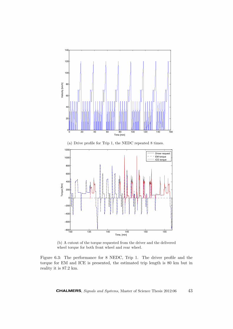
0 20 40 60 80 100 120 140 1600

20

40

60

80

100

120

140

Time [min]

Velo

city

[km

/h]

(a) Drive profile for Trip 1, the NEDC repeated 8 times.

130 135 140 145 150 155−800

−600

−400

−200

0

200

400

600

800

1000

1200

Time, [min]

Torq

ue [N

m]

Driver requestEM torqueICE torque

(b) A cutout of the torque requested from the driver and the deliveredwheel torque for both front wheel and rear wheel.

Figure 6.3: The performance for 8 NEDC, Trip 1. The driver profile and thetorque for EM and ICE is presented, the estimated trip length is 80 km but inreality it is 87.2 km.


0 10 20 30 40 50 60 70 80 9010

20

30

40

50

60

70

80

90

Distance, [km]

Stat

e of

Cha

rge,

[%]

Reference SoCSoCNominal SoC

Figure 6.4: The SoC trajectories for both the ECMS with blended discharge andthe nominal control strategy the CDCS strategy for Trip 1.

0 20 40 60 80 100 120 140 1600

0.1

0.2

0.3

0.4

0.5

0.6

0.7

0.8

0.9

1

Time [min]

Dis

sipa

ted

elec

trica

l ene

rgy

[nor

mal

ized

uni

ts]

NominalECMS

Figure 6.5: The accumulated battery losses Trip 1. The result is presented innormalized units, the ECMS, with blended discharge, is ∼ 30 % better.


0 10 20 30 40 50 60 70 80 90 1000

20

40

60

80

100

120

Time [min]

Velo

city

[km

/h]

(a) Drive profile for Trip 2.

70.5 71 71.5 72 72.5 73 73.5 74 74.5 75−400

−200

0

200

400

600

800

1000

1200

Time, [min]

Torq

ue [N

m]


(b) A cutout of the torque requested from the driver and the deliveredwheel torque for both front wheel and rear wheel. Note that this is in thehigh speed part.

Figure 6.6: The performance for Trip 2. The driver profile and a cutout of the re-quested torque and the torque for the EM and the ICE is presented. The estimatedtrip length is 67 km but in reality it is 67.94 km.


0 10 20 30 40 50 60 7010

20

30

40

50

60

70

80

90

Distance, [km]

Stat

e of

Cha

rge,

[%]


Figure 6.7: The SoC trajectories for Trip 2 for both the ECMS with blendeddischarge and the nominal, rule-based CDCS strategy.

0 10 20 30 40 50 60 70 80 90 1000

0.1

0.2

0.3

0.4

0.5

0.6

0.7

0.8

0.9

1

Time, [min]

Dis

sipa

ted

elec

trica

l ene

rgy

[nor

mal

ized

uni

ts]

RBECMS

Figure 6.8: The accumulated battery losses for Trip 2. The result is presented innormalized units, the ECMS, with blended discharge, is ∼ 5 % better.


0 50 100 1500

20

40

60

80

100

120

140

Time [min]

Velo

city

[km

/h]

(a) Drive profile for Trip 4s.

65 65.5 66 66.5 67 67.5 68 68.5 69 69.5 70−100

−50

0

50

100

150

200

250

300

Time, [min]

Torq

ue, [

Nm

]


(b) A cutout of the torque requested from the driver and the deliveredwheel torque for both front wheel and rear wheel.

Figure 6.9: The performance for Trip 4. The driver profile and a cutout of thetorque. The estimated trip length is 156 km the true distance is 156.39 km.


0 20 40 60 80 100 120 140 16010

20

30

40

50

60

70

80

90

Distance, [km]

Stat

e of

Cha

rge,

[%]


Figure 6.10: The SoC trajectories for Trip 4 for both the ECMS with blendeddischarge and the nominal, rule-based CDCS strategy.

0 50 100 1500

0.1

0.2

0.3

0.4

0.5

0.6

0.7

0.8

0.9

1

Time [min]

Dis

sipa

ted

elec

trica

l ene

rgy

[nor

mal

ized

uni

ts]

NominalECMS

Figure 6.11: The accumulated battery losses for Trip 4. The result is presented innormalized units, the ECMS, with blended discharge, is ∼ 30 % better.


7 Analysis

In the following section, an analysis of the respective results is presented.

7.1 Fuel consumption

The results in Table 6.4 are indicating that the ECMS strategy perform better forall of the 8 drive cycles evaluated, reducing the fuel consumption in the range of1− 9 % and by 4.2 % on average. These figures are presented without consideringthe difference in SoC at the end of the trip between the two strategies compared. Acorrection would be to multiply the remaining energy quantity by the average of theequivalence factor (as a measure of efficiency), according to Equation (6.6). Thereduction in fuel consumption would then span between 0− 12 % but the averageremains at 4.2 %. Note that this is an estimation of the corrected fuel consumption,the true efficiency of the supposed engine operation remains unknown.

It can be noted that the fuel consumption for ECMS with CDCS is also reducedbut not so much as for the blended discharge strategy. The change varied from+3 % to −7 % (uncorrected) but yet made a 1.7 % reduction on average, thecorrected average is 1.0 %. For Trip 1, while using CDCS, the fuel consumptionincreased, possibly because the nominal controller is tuned specifically towardsthis drive cycle while the ECMS algorithm is tuned completely towards a blendedmode discharge. The parameters s0, K and Pstart can be modified for such tuning.

7.2 Engine start cost

The introduction of the perceived engine start cost, Pstart, made a significant dif-ference in reducing the number of engine starts. Further tuning of Pstart consistingof varying the start cost for different vehicle speed intervals contributed to a largeimpact in fuel consumption, resulting in a relative reduction for blended modedischarge for all of the 8 drive cycles that were evaluated. The main advantagethat a variable engine start cost brings, besides reducing the number of enginestarts, is also the ability to prioritize the decision to select the power split basedon efficiency rather than selection due to temporary SoC deviation. This can bedescribed as to locally adjust the SoC reference up or down slightly to overridethe SoC feedback functionality for a certain SoC deviation, based on informationknown externally (e.g. electric propulsion is preferred at low speed).


7.3 Battery operation

Evaluation of battery operation in terms of battery life can be done with respect toa number of parameters [11], of which a few of them are analyzed here. The resultspresented in Table 6.4 show comparisons of RMS current, battery power losses andtotal current throughput. Another parameter that affects battery life is the timespent at low SoC levels, which can be observed from the SoC discharge trajectoriesdisplayed in figures from Section 6.3. All results are analyzed with respect to theECMS control strategy in relation to the nominal rule-based strategy with a CDCSdischarge strategy.

Starting with the battery RMS currents, iRMS , which were found to be reduced,on average, by 8.5 % for blended mode and 3.4 % for the ECMS using the CDCSstrategy. The resulting battery power losses, Pbatt,loss,avg, were on average reducedby 15.6 % in blended mode and 6.7 % for CDCS. Reductions in blended modedriving is an expected consequence from the ability of the EM to operate at lowercurrent levels by avoiding suboptimal operating points, as higher currents inducemore losses, according to Equation (6.3). As a side note, it may be expected thatpower losses would be proportional to the square of the RMS currents. The reasonof why the results show a slight deviation in this regard is because the batteryresistances were not identical between the two cases, which is why it does not addup. Another important reason for the power loss reduction is the higher averagebattery voltage at which the EM operates at during blended mode, despite beingused frequently, which lowers the necessary current for a specific power accordingto P = UI.

Additionally, the total electric energy cycled through the battery, Ahbatt, wasalso found lower for both discharge strategies. Blended mode resulted in a 10.9 %reduction on average and CDCS made a 8.6 % reduction. This is illustrated inFigures 6.5, 6.8 and 6.11. The reductions presented above are all contributors tomaintaining a long battery life, as well as the shorter time spent at low SoC levelswhich has only been presented in figures.

7.4 Drive cycle influence

By comparing the fuel consumption results in Table 6.4 for Trips 2 and 3, it canbe noted that there is a difference in consumption between the ECMS controlledstrategies compared to the rule-based case. It is notable because the only differenceis within the order of two different speed segments. Trip 2, see Figure A.2, beginswith a low speed segment and ends with a high speed segment. However, Trip 3,see Figure A.3, begins with the same high speed part of Trip 2 and ends with thelow speed part of Trip 2. The fact that the nominal strategy varies significantly infuel consumption compared to ECMS despite that the same drive cycles are usedsuggests that the CDCS discharge strategy is quite sensitive to such “unfortunate”drive cycle designs. The ECMS control strategy with blended discharge could thenbe considered more robust to such variation in drive cycle design.

When looking at whether high or low speeds in general influence one strategy or


the other, some small indications can be observed. The rule-based control strategywith CDCS performs its best, close to ECMS, for drive cycles with more low speedsegments, for example Trip 6. When it comes to high speed segments, for exampleTrip 5, ECMS for both discharge strategies perform significantly better (∼ 4 %)than the rule-based control strategy with CDCS.

7.5 Equivalence factor

The method used to determine the equivalence constant sblended in Section 5.3 hasbeen found to provide suitable constants for blended mode operation, resultingin satisfactory SoC trajectories without using too much SoC feedback. It is alsoefficient as it only requires a single run per drive cycle. For the ECMS control underthe CDCS discharge strategy, the equivalence constant s0 used during depletionwas the same as for blended mode discharge. If the equivalence constant wouldhave been tuned specifically (slightly lower) for this discharge strategy instead(during CD mode), the results might have differed slightly in favor to ECMS.

The sustain constant ssustain was found based on the method of sweepingdifferent power split ratios and evaluating the energy for each of them. This valuewas only based on one simulation with the NEDC drive cycle, which is shorterthan the AER. The variation of s(t), seen in Appendix C, at the end is quitehigh, this is mainly due to the slope of the tangent function, which is higher insustaining mode, i.e. when the estimated distance Dtot has been exceeded or if theSoC target has been reached. During normal operation, s(t) does not exceed thelimits but it may show some variation.


8 Discussion

The results are in general satisfactory and to some extent also expected. However,there are some aspects that were not clear after the analysis and need furtherdiscussion.

8.1 Reducing the fuel consumption

The blended mode discharge strategy operating under ECMS has shown a reduc-tion in fuel consumption. This is possible mainly thanks to a more selective use ofthe EM and ICE by matching them to suitable operating points. Such matchingleads to increased fuel efficiency as well as lowered electric power losses. Anothercontributing factor is the engine start penalty cost which helped reducing the num-ber of engine starts as well as locally reducing the influence of the SoC dependence,avoiding suboptimal operating points.

It can be seen though, that fuel consumption was not reduced for all casesinvestigated. Some particular drive cycles resulted in increased fuel consumptionfor the CDCS strategy under ECMS control. This might depend on the fact thatthe ECMS algorithm was not at all tuned for the CDCS case. If some tuningof both s0 and Pstart were to be made, the results might turn out differently.Additionally, the nominal strategy uses the ISG at some points while it is not usedat all in the ECMS control algorithm studied in this thesis. This can possibly bewhat is influencing the results. The use of the ISG may lead to either higher orlower fuel consumption for the ECMS control strategy depending on how well it isutilized. The utilization of the ISG might as well explain why the nominal CDCSalternative is better sometimes and sometimes not.

8.2 Battery life

The stress of the battery was lowered when using the ECMS algorithm to solvethe control problem, for both blended and CDCS battery discharge. This is anadvantage because, if the battery losses are higher, the battery will need morecooling which means that more auxiliary power has to be used for battery cooling.Indirectly, this will eventually lead to increasing fuel consumption due to the extraamount of battery energy consumed for the auxiliary power demaded. In thevehicle model used, the cooling power is not modeled and temperature effects aretherefore not taken into account. The battery losses are lower with the ECMSalgorithm which would also lead to lower cooling power of the battery.


When attempting to evaluate the possible impact that the improved batteryusage may bring to prolonging battery life, there are at least a few indicative factorsto consider. According to [11], the effective Ah-throughput, Aheff , proportionalto battery life, may be estimated as follows

Aheff =

wEnEAhE (8.1)

where the index E denotes the event at which an Ah-throughput, AhE , is drawn.The factors wE and nE correspond to the severity of the event and the numberof such events, respectively. This simple estimation may suggest that a 10.9 %average reduction in Ah-throughput would also increase the effective battery lifeby ∼ 12.2 %. This is under the assumption that wE and nE are constant. How-ever, with lowered RMS currents wE would be lowered as well, suggesting furtherimprovements of battery life.

According to [17], the charge rate of the battery can strongly influence itslifetime. As an example, the cycle life was increased by 100 % by reducing thecharging rate from 3.75 C-rate to 2 C-rate, where C-rate corresponds to the currentnormalized with battery capacity. In this example it would be equivalent to fullycharging the battery in 16 and 30 minutes respectively. This suggests that itmay perhaps be more important to consider how quickly the battery is rechargedbetween trips before analyzing the usage during actual driving. The observedimprovement in battery operation during driving is likely to have a significantpositive impact if the battery is also recharged slowly between each trip, whereasfast recharge induces more stress to the battery which may seriously limit therelative impact of this improvement.

8.3 Modeling errors

The quite coarse modeling of the ICE startup sequence has been identified as oneissue that may induce errors. A modeling problem when the engine is started canbe seen, for example in Figure 6.6 where the torque of the ICE is negative duringstartup. This could perhaps be due to incorrect modeling of the transmission con-trol. Given that the ECMS solution turns the ICE on and off many times over adrive cycle, the loss will grow with the number of engine starts and become quitesignificant. The number of ICE startups aside, both discharge strategy implemen-tations are using the vehicle model in similar ways, suggesting that modeling errorswould have equivalent impact on both solutions and thereby cancel each other.

Another issue related to modeling may be the feedback gain of the simulateddriver, which is modeled by a PID-controller. A potential problem may be thathigh power demands may trigger unnecessarily high and short peaks of batterypower costs, causing the power split to shift to ICE propulsion more frequently.This problem may be solved by applying a time dependent ICE startup cost thatdecreases after some time once an engine start has been requested, or by decreasingthe feedback gains in the driver model.

In the model used for the ECMS algorithm some power losses was neglected,such as the power losses in the transmission and the ISG inverter losses. If the


neglected power losses had been taken into account, the ECMS performance couldperhaps have been improved.

8.4 Estimation of equivalence factor

As shown in Table 6.2, the equivalence factor is not very sensitive to the speedproperties of the drive cycle but varies more depending on the trip length. Initialand final SoC levels affect the equivalence factor in the same way. By sweeping alarger set of drive cycles with ranging trip lengths and SoC limits, these parameterscan present a clearer relation and help finding a function for a suitable s0 to bedetermined. A better model for estimating s0 may also reduce the fuel consumptionfurther, due to less SoC feedback activity in s(t). This is because SoC feedback canshade the normal cost calculation and thereby dismiss an otherwise good operatingpoint for a less efficient one, simply due to temporary SoC deviation. It seems thatthe schedule used for selecting different ICE startup penalty costs is an effectivecomplement to the equivalence factor in avoiding this problem.

8.5 Estimation errors

If the estimated value on the trip length Dtot is changed slightly, the result of theECMS is also changed. This result was also proven in [3]. This means that if theexact trip length would have been used the fuel consumption could possibly havebeen reduced further. The distance was underestimated because it is not satisfyingto end the trip with unconsumed battery energy that should have been used forpropulsion.


9 Future work

Concepts and ideas that were either beyond time constraints to investigate or outof scope for the thesis but yet interesting for future developments of the solutionare presented below.

9.1 Better engine start cost

One factor that showed to be of high importance for fuel consumption is the setof values used for the engine start penalty, Pstart. When simulations were madeto determine these values it was noticed that even small changes had a significantimpact on the fuel consumption. There is still a large uncertainty in how close tooptimal this variable startup cost is. This is mainly because it has been designedbased on only two drive cycles in order to provide for validation and avoid “cyclebeating” (specific drive cycle tuning). With a more sophisticated function for thispenalty, preferably with inputs such as current SoC, speed and requested torque, apenalty more close to optimal could be estimated. It would be beneficial to couplethis cost to the existing hardware (EM and ICE) and allow for easy modificationwith new system parameters when being applied into a different vehicle. This isbecause extensive tuning for every change of system is to be avoided.

9.2 Mechanical energy reference

Using distance to form the desired SoC discharge trajectory is not likely the bestreference. As a part of future developments of the ECMS solution, the amountof information known a priori could perhaps be extended further. Informationabout the topography, expected speed limits and traffic situation for a specifiedtrip between points A and B could be used to estimate the total mechanical energyrequired by the vehicle during the trip. By using the mechanical energy neededfor propulsion as a basis for the SoC reference instead of the distance, it may bepossible to achieve an even more efficient discharge path.

9.3 Route recognition

In order to aid the estimation of the mechanical energy reference mentioned be-fore, some sort of route recognition method could be employed [3], unless the driverhimself/herself feels like dialing the exact destination on the integrated GPS nav-igator. Based on logged data from earlier trips, some sort of route recognitionalgorithm can be used to find the most commonly occurring trips. Once a trip hasbeen identified, information provided by services such as Google Maps R can beused to effectively estimate the trip length, time to travel and even the impact oftraffic.


9.4 ECMS model update

An update of the ECMS model with the previously neglected losses from compo-nents such as ISG inverter, transmission efficiency, idle losses of the ICE as wellas varying auxiliary power, could be done for a better evaluation of the ECMScontrol strategy.

The ISG should also be included in the ECMS algorithm so that an additionaldegree of freedom can be utilized, allowing further improvements in ICE operat-ing point selection. This could bring benefits to battery operation by providing“cheap” recharge opportunities.

The ECMS algorithm uses for-loops and to be able to decrease the compu-tational power, the loops can be exchanged to matrix operations. Some of thecalculations in the algorithm can also be optimized for faster computations by us-ing more efficient algorithms. Another impact of the computational power is howoften the ECMS control should update the power split ratios. The updates arecurrently made every 10 ms. By lowering the update rate to e.g. 1 s, the resultmay provide faster computations. Further investigation of such a change shouldbe made to see how it affects the accuracy of the model.

Another consideration that could be added to the ECMS algorithm is thevarious emissions; NOx, CO2, CO, HC and particles. Also, for a more completeanalysis of the impact of ECMS and blended mode discharge, the componentwear, specifically in the ICE, should also be considered while formulating the costfunction.

9.5 ECU implementation

The objective of real-time implementation for the ECU was not fulfilled. It wouldnot be practical to transfer the current ECMS algorithm due to the long com-putational times required, but some investigation has been made of how such animplementation could be done. By using surface fitting algorithms, the ECMSoptimization could be included in an ECU as lookup tables. There are toolboxesfor surface fitting in Matlab R for example the toolbox ARESLab [18], whichcan be used for generation of such surfaces.


10 Conclusions

Upon finishing the investigations of alternative strategies for control and dischargeof electric energy in a hybrid powertrain, the following conclusions could be made.

• Fuel consumption was reduced by 4.2 % on average for all tested drive cycleswith a blended discharge under ECMS control, compared to the rule-basedCDCS discharge strategy, which a satisfactory result. For the case of ECMScontrol with a CDCS discharge strategy, the fuel consumption was reducedby 1.0 % on average instead. Both figures reflect the corrected fuel con-sumption.

• An engine start penalty cost is important when it comes to reducing thenumber of engine starts and avoiding suboptimal operating points, whichotherwise contributes to a higher fuel consumption. Consequently it is alsoimportant to consider the accuracy of the model during the engine startprocess.

• Battery power losses and Ah-throughput were reduced with the ECMS con-trol strategy for both the CDCS and the blended discharge strategy. Theseare both beneficial for improving the battery life, especially if the rechargerate (current) from the grid is not too high.

• A less time consuming way of determining an equivalence factor was found,which is beneficial for large and complex simulation models.

• The speed segment layout of drive cycles had certain effects on the rule-basedCDCS discharge strategy, where city driving first and highway afterwards(similar to NEDC) is significantly more beneficial than the other way around.With ECMS there is more robustness to such arrangements in the speedsegment layout.


References

[1] Vagverket, “Hallbart resande,” 2006. http://publikationswebbutik.vv.

se/upload/1543/88587_hallbart_resande_utg_2.pdf Retrieved 2012-04-12.

[2] Swedish Institute for Transport and Communications Analysis, “Res 2005-2006 the national travel survey,” 2007.

[3] V. Larsson, “On discharge strategies for plug-in hybrid electric vehicles,”licentiate thesis, Signal and System, Chalmers University of Technology,Goteborg, Sweden, 2012.

[4] A. Sciarretta, M. Back, and L. Guzzella, “Optimal control of parallel hybridelectric vehicles,” IEEE Transactions on Control Systems Technology, vol. 12,pp. 352–363, May 2004.

[5] C. Zhang and A. Vahidi, “Real- time optimal control of plug-in hybrid vehicleswith trip preview,” in American Control Conference, pp. 6917–6922, 2004.

[6] V. Freyermuth, E. Falles, and A. Rousseau, “Comparison of powertrain config-uration for plug-in hevs from a fuel economy perspective,” SAE International,2007.

[7] L. Guzzella and A. Sciaretta, Vehicle Propulsion Systems. Berlin Heidelberg:Springer Verlag, 2nd ed., 2007.

[8] Embedded Success dSPACE, “Targetlink R.” http://www.dspace.com/en/

inc/home/products/sw/pcgs/targetli.cfm Retrieved 2012-05-31.

[9] B. He and M. Yang, “Optimization-based energy management of series hybridvehicles considering transient behavior,” Int. J. Alternative Propulsion, vol. 1,no. 1, pp. 79–96, 2006.

[10] T. van Keulen and et al., “Design, implementation, and experimental val-idation of optimal power split control for hybrid electric trucks,” ControlEngineering Practice, vol. 20, pp. 547–558, 2012.

[11] H. Wenzl and et al., “Life prediction of batteries for selecting the technicallymost suitable and cost effective battery,” Journal of power sources, vol. 144,pp. 378–384, 2005.

[12] C. Musardo and G. Rizzoni, “A-ECMS: An adaptive algorithm for hybridelectric vehicle energy management,” in 44th IEEE Conference on Decisionand Control, vol. 11, pp. 1816–1823, Oct. 2005.

[13] D. S. Naibu, Optimal Control Systems. CRC Press LLC, 1st ed., 2003.


[14] S. Stockar, V. Marano, M. Canova, and G. Rizzoni, “Energy-optimal con-trol of plug-in hybrid electric vehicles for real-world driving cycles,” IEEETransactions on vehicular Technology, vol. 60, no. 7, pp. 2949–2962, 2011.

[15] P. Tulpule, V. Marano, and G. Rizzoni., “Energy management for plug-inhybrid electric vehicles using equivalent consumption minimisation strategy,”Int. J. Electric and Hybrid Vehicles, vol. 2, no. 4, pp. 329–350, 2010.

[16] L. Johannesson, S. Pettersson, and B. Egardt, “Predicted energy managementof a 4QT series-parallel hybrid electric bus,” Control Engineering Practice,vol. 17, no. 12, pp. 1440–1453, 2009.

[17] J. Groot, “State-of-health estimation of li-ion batteries: Cycle life test meth-ods,” licentiate thesis, Energy and Environment, Chalmers University of Tech-nology, Goteborg, Sweden, 2012.

[18] G. Jekabsons, “ARESLab: Adaptive regression splines toolbox for matlab/oc-tava,” 2011. http://www.cs.rtu.lv/jekabsons/ Retrived 2012-04-24.


Appendices

A Drive cycles

0 20 40 60 80 100 120 140 1600

20

40

60

80

100

120

Time [min]

Velo

city

[km

/h]

Figure A.1: Trip 1. New European Drive Cycle (NEDC), repeated 8 times, withpredicted driving distance of 80 km.

0 10 20 30 40 50 60 70 80 90 1000

20

40

60

80

100

120

Time [min]

Velo

city

[km

/h]

Figure A.2: Trip 2. Logged cycle with a predicted driving distance of 67 km.

, Signals and Systems, Master of Science Thesis 2012:06 I

0 10 20 30 40 50 60 70 80 90 1000

20

40

60

80

100

120

Time [min]

Velo

city

[km

/h]

Figure A.3: Trip 3. Logged cycle with a predicted driving distance of 67 km.This drive cycle contains the same profile as Trip 2, but the high speed segmentis placed to the beginning instead.

0 50 100 1500

20

40

60

80

100

120

Time [min]

Velo

city

[km

/h]

Figure A.4: Trip 4. A logged drive cycle with a predicted driving distance of 156km.

, Signals and Systems, Master of Science Thesis 2012:06 II

0 10 20 30 40 50 60 700

20

40

60

80

100

120

140

Time [min]

Velo

city

[km

/h]

Figure A.5: Trip 5. Logged highway cycle with predicted driving distance ∼ 92km.

0 50 100 1500

10

20

30

40

50

60

70

80

90

100

Time [min]

Velo

city

[km

/h]

Figure A.6: Trip 6. Logged cycle with predicted driving distance 92 km.

, Signals and Systems, Master of Science Thesis 2012:06 III

0 5 10 15 20 25 30 35 40 450

20

40

60

80

100

120

Time [min]

Veloc

ity [k

m/h]

Figure A.7: Trip 7. Drive cycle used for evaluation with distance ∼ 60 km.

0 10 20 30 40 50 60 70 80 900

20

40

60

80

100

120

Time [min]

Veloc

ity [k

m/h]

Figure A.8: Trip 8. Drive cycle used for evaluation with distance ∼ 120 km.

, Signals and Systems, Master of Science Thesis 2012:06 IV

B List of inputs and constants to the ECMSalgorithm

d time dependentDtot constantSoC time dependentSoCfinal constantSoCinit constantSoCref time dependents0 constantK constantTwhl time dependentωwhl time dependentPaux constantgrGB time dependentgrEM constantgrbelt constantηgr,EM constantηgr,belt constantmfuel lookup tablePbatt,loss time dependentPfuel,start constantPEM,El time dependentPISG,El time dependentPaux constantPfuel,ICE time dependentPfuel time dependentPbatt time dependentQlhv constantVbatt time dependentu1 constantu2 constant

, Signals and Systems, Master of Science Thesis 2012:06 V

, Signals and Systems, Master of Science Thesis 2012:06 VI

C The variation of s(t)

0 20 40 60 80 100 120 140 1600

2

4

6

8

10

12

Time, [min]

s(t),

[−]

Figure C.1: s(t) for Trip 1. The predicted trip length is shorter than the true one,therefore the large changes at the end of the trip.

0 10 20 30 40 50 60 70 80 90 1001

1.5

2

2.5

3

3.5

4

4.5

5

5.5

Time, [min]

s(t),

[−]


, Signals and Systems, Master of Science Thesis 2012:06 VII

0 10 20 30 40 50 60 70 80 90 1002

3

4

5

6

7

8

9

10

11

12

Time, [min]

s(t),

[−]


0 50 100 1502

3

4

5

6

7

8

Time, [min]

s(t),

[−]


, Signals and Systems, Master of Science Thesis 2012:06 VIII

0 10 20 30 40 50 60 701

1.5

2

2.5

3

3.5

4

4.5

Time, [min]

s(t),

[−]


0 50 100 1501

2

3

4

5

6

7

8

9

Time, [min]

s(t),

[−]


, Signals and Systems, Master of Science Thesis 2012:06 IX

0 10 20 30 40 50 60 70 80 900.5

1

1.5

2

2.5

3

3.5

4

4.5

Time, [min]

s(t),

[−]


, Signals and Systems, Master of Science Thesis 2012:06 X

Energy Management Strategies for Plug-in Hybrid Electric ...

Documents

Transcript of Energy Management Strategies for Plug-in Hybrid Electric ...