
ENVIRONMENTAL IMPACT OF PLUG IN HYBRID ELECTRIC VEHICLES ...
174
ENVIRONMENTAL IMPACT OF PLUG‐IN HYBRID ELECTRIC VEHICLES IN MICHIGAN by Aaron Camere Caroline de Monasterio Jason MacDonald Allison Schafer A project submitted in partial fulfillment of the requirements for the degree of Master of Science (Natural Resources and Environment) at the University of Michigan August 2010 Faculty advisors: Dr. Gregory Keoleian (SNRE/CSS) Dr. Jarod Kelly (SNRE/CSS)
Transcript of ENVIRONMENTAL IMPACT OF PLUG IN HYBRID ELECTRIC VEHICLES ...

ENVIRONMENTAL IMPACT OF PLUG‐IN HYBRID ELECTRIC VEHICLES IN MICHIGAN
by
Aaron Camere Caroline de Monasterio
Jason MacDonald Allison Schafer
A project submitted
in partial fulfillment of the requirements for the degree of Master of Science
(Natural Resources and Environment) at the University of Michigan
August 2010
Faculty advisors: Dr. Gregory Keoleian (SNRE/CSS) Dr. Jarod Kelly (SNRE/CSS)

THIS PAGEINTENTIONALLY LEFT
BLANK

Center for Sustainable Systems University of Michigan, Ann Arbor
MPSC PHEV Pilot Study Page i 07/30/2010
Abstract
The environmental and electric utility system impacts from plug‐in hybrid electric vehicle (PHEV)
infiltration in Michigan were examined from years 2010 to 2030 as part of the Michigan Public Service
Commission’s (MPSC) PHEV pilot project. Total fuel cycle energy consumption, greenhouse gas and
criteria air pollutant emissions for Michigan’s light duty vehicle fleet were analyzed, as well as gasoline
displacement due to the shift to electrified travel.
PHEVs consume both liquid fuel and grid electricity for propulsion. While this fueling strategy
can significantly reduce gasoline consumption and related emissions, it is important to understand the
impacts that these PHEVs have on the electrical system and its associated emissions. A MATLAB® model
was developed to quantify the regional emissions and energy use of this interaction for Michigan.
Each year the model examined vehicle charging behavior, PHEV sales infiltration, changes to the
electric grid, and electricity dispatch. Individual PHEV energy consumption was determined from a
database of actual vehicle trips, and scaled to the number of on‐road PHEVs. The electricity to charge
PHEVs was added to Michigan’s baseline hourly electrical demand and new generating capacity was
added to the grid to meet renewable portfolio standards and capacity reserve mandates. Lastly,
generating assets were dispatched to serve the load, and total fuel cycle (TFC) emissions were
calculated. Several scenarios were developed to capture the range of possible outcomes examining
PHEV infiltration, charging behaviors, and future grid mixes.
In all scenarios, an increased number of PHEVs led to decreased statewide GHG emissions,
ranging from a 0.4% to 10.7% reduction in 2030, and displaced from 0.5 to 9 billion gallons of gasoline
from 2010‐2030. Depending on the scenarios employed and allocation method, The emissions intensity
of PHEV travel in 2030 ranged from 294 and 187 gCO2e per mile. Substituting nuclear generators for
some of Michigan’s predominately coal baseload power plants had a large effect on reducing emissions,
a 40% reduction in annual electricity sector GHG emissions between 2009 and 2030, and reduced PHEV
emissions intensity up to 22%. Criteria air pollutant emissions were reduced in most scenarios.
However, SOX emissions could increased with the addition of PHEVs.

Center for Sustainable Systems University of Michigan, Ann Arbor
MPSC PHEV Pilot Study Page ii 07/30/2010
Acknowledgements
This research study would not have been possible without the support, both technical and personal, of
many individuals. We would especially like to thank our faculty advisors, Gregory Keoleian, Jarod Kelly
and Ian Hiskens from the University of Michigan. Additionally, we would like to thank former faculty
members Duncan Callaway, presently at University of California, Berkeley, and John Sullivan, presently
at Argonne National Labs. Finally, our thanks go out to Yujia Zhou and Norb Podwoiski and the rest of
the Market Intelligence group at DTE Energy for all their valuable assistance and guidance.

Center for Sustainable Systems University of Michigan, Ann Arbor
MPSC PHEV Pilot Study Page iii 07/30/2010
Table of Contents Abstract .......................................................................................................................................................... i
Acknowledgements ....................................................................................................................................... ii
List of Figures .............................................................................................................................................. vii
List of Tables ................................................................................................................................................. x
List of Acronyms and Key Terms ................................................................................................................. xii
Nomenclature .............................................................................................................................................xiii
1. Executive Summary ............................................................................................................................... 1
1.1 Modeling Methodology and Scenarios ......................................................................................... 3
1.1.1 PHEV Energy Consumption ................................................................................................... 3
1.1.2 Fleet Infiltration .................................................................................................................... 5
1.1.3 Electric Grid ........................................................................................................................... 6
1.2 Key Findings & Conclusions ........................................................................................................... 7
1.3 Recommendations and Future Work .......................................................................................... 11
2. Introduction ........................................................................................................................................ 12
2.1 Previous Research and Context .................................................................................................. 12
2.2 Research Objectives .................................................................................................................... 16
2.3 Scope and System Definition ...................................................................................................... 17
2.4 Report Organization .................................................................................................................... 19
3. Methodology ....................................................................................................................................... 20
3.1 PHEV Energy Consumption Model .............................................................................................. 20
3.1.1 PHEV Characterization ........................................................................................................ 20
3.1.2 The National Household Travel Survey ............................................................................... 21
3.1.3 Vehicle Trip‐days ................................................................................................................. 22
3.1.4 Modeling PHEV Energy Consumption ................................................................................. 22
3.1.5 Charging Parameters and Constraints ................................................................................ 26
3.1.6 Aggregation and Normalization .......................................................................................... 28
3.2 Michigan Light Duty Vehicle Fleet Modeling .............................................................................. 30
3.2.1 Distribution of vehicles ....................................................................................................... 30
3.2.2 Conventional Vehicle Consumption .................................................................................... 31

Center for Sustainable Systems University of Michigan, Ann Arbor
MPSC PHEV Pilot Study Page iv 07/30/2010
3.2.3 Plug‐in Vehicle Consumption .............................................................................................. 32
3.3 Electricity Generation Capacity Changes .................................................................................... 32
3.3.1 Generating Asset Retirements ............................................................................................ 33
3.3.2 Generating Asset Additions to Meet Renewable Portfolio Standards ............................... 34
3.3.3 Generating Asset Additions for Reserve Margin ................................................................. 35
3.4 Electricity Dispatch Modeling ..................................................................................................... 36
3.4.1 Wind Assets ......................................................................................................................... 39
3.4.2 Hydroelectric Assets ............................................................................................................ 41
3.4.3 Capacity Factor Dispatch ..................................................................................................... 45
3.4.4 Economic Dispatch .............................................................................................................. 48
3.5 Emissions & Life Cycle Metrics .................................................................................................... 49
3.5.1 Electricity Generation Energy and Emissions ...................................................................... 49
3.5.2 On‐Road Vehicle Energy and Emissions .............................................................................. 51
3.5.3 Allocation Methods ............................................................................................................. 52
4. Scenarios ............................................................................................................................................. 55
4.1 PHEV Fleet Infiltration Scenarios ................................................................................................ 55
4.3 Electricity Generating Capacity Scenarios ................................................................................... 58
4.4 Charging Scenarios ...................................................................................................................... 60
4.5 Electricity Dispatch Scenarios ..................................................................................................... 62
4.6 Simulations Analyzed .................................................................................................................. 63
5. Results and Discussion ........................................................................................................................ 65
5.1 PHEV Energy Consumption Model Results ................................................................................. 65
5.1.1 Daily Variation in PHEV Consumption ................................................................................. 65
5.1.2 Charging Scenario Analysis ................................................................................................. 67
5.1.3 Minimum Dwell time and Charge Onset Delay ................................................................... 73
5.2 Greenhouse Gas Emissions ......................................................................................................... 73
5.2.1 Fleet Infiltration Implications .............................................................................................. 74
5.2.2 Electricity Generation Capacity Implications ...................................................................... 81
5.2.3 PHEV Charging Behavior Implications ................................................................................. 87
5.2.4 Electricity Dispatch Method ................................................................................................ 88

Center for Sustainable Systems University of Michigan, Ann Arbor
MPSC PHEV Pilot Study Page v 07/30/2010
5.3 Criteria Air Pollutant Emissions ................................................................................................... 92
5.3.1 Total system air pollutant emissions .................................................................................. 93
5.3.2 Transportation sector air pollutant emissions .................................................................... 96
5.3.3 Criteria air pollutants (comparison with GHGs) .................................................................. 99
5.4 Total Fuel Cycle Energy ............................................................................................................. 100
5.5 Gasoline Displacement ............................................................................................................. 102
5.6 Comparison to other studies .................................................................................................... 103
6. Conclusions and Recommendations ................................................................................................. 105
6.1 Key Findings .............................................................................................................................. 105
6.2 Recommendations .................................................................................................................... 110
6.3 Future Work .............................................................................................................................. 111
Appendix A. Initial assets matrix ............................................................................................................... 114
Appendix B. Scripted fleet retirements and additions .............................................................................. 120
Appendix C. Future baseline consumer demand ...................................................................................... 123
Appendix D. Fuel prices for Economic Dispatch ....................................................................................... 125
Appendix E. Vehicle size class mapping .................................................................................................... 126
Appendix F. Plug‐in electric hybrid vehicle characteristics ...................................................................... 127
Appendix G. Emissions allocation example from MEFEM ........................................................................ 133
Appendix H. Additional PECM Results ...................................................................................................... 138
Effect of Battery size ......................................................................................................................... 138
Effect of Size class ............................................................................................................................. 139
Additional Load lineups ..................................................................................................................... 142
Appendix I. Additional Greenhouse Gas Emissions Results ...................................................................... 150
Appendix J. Additional Criteria Pollutant Results ..................................................................................... 151
References ................................................................................................................................................ 156

Center for Sustainable Systems University of Michigan, Ann Arbor
MPSC PHEV Pilot Study Page vi 07/30/2010
List of Figures
Figure 1. High level system diagram ............................................................................................................. 2
Figure 2. Electric system demand in Michigan, one week in January, 2030. ............................................... 4
Figure 3. PHEV infiltration rates, 2010 ‐ 2030 ............................................................................................... 5
Figure 4. Load duration curve showing hydro and wind dispatch. ............................................................... 7
Figure 5. Total GHG emissions for the year 2030 for all infiltration scenarios (EG1, CH1) ........................... 8
Figure 6. Change in total system emissions between FI1 and FI4 (EG1, CH1, 2030) .................................... 9
Figure 7. Percentage of travel driven electrically by charging scenario ....................................................... 9
Figure 8. Per mile greenhouse gas emissions for each charging scenario .................................................. 10
Figure 9. Project organization diagram of MPSC PHEV pilot project .......................................................... 17
Figure 10. High level schematic of overall system structure ...................................................................... 18
Figure 11. Vehicle trip‐day depictions of NHTS data .................................................................................. 22
Figure 12. Energy SOC plot for sample vehicle trip‐day 1 ........................................................................... 24
Figure 13. Energy SOC plot showing operational mode ............................................................................. 25
Figure 14. Iterative trip‐day eSOC profile for sample vehicle 3 .................................................................. 25
Figure 15. Iterative trip‐day eSOC plot for sample vehicle 5 ...................................................................... 26
Figure 16. Charging for profile for each of the sample vehicle trip‐days ................................................... 29
Figure 17. Weighted, aggregated, and normalized charging profile for sample vehicle trip‐days ............. 29
Figure 18. Normalized aggregate charging profile for a complete NHTS sample ....................................... 30
Figure 19. RPS fuel mix for capacity additions. ........................................................................................... 35
Figure 20. Load duration curve example with 3 plants............................................................................... 38
Figure 21. System diagram for electricity dispatch ..................................................................................... 39
Figure 22. The 13 Michigan sites simulated by the NREL wind integration dataset .................................. 40
Figure 23. Sample of normalized wind power generation curve (week in Jan. and June) ......................... 41
Figure 24. Wind dispatch’s effect on system demand ................................................................................ 41
Figure 25. Example of the sorted dispatch shown for a very large hydroelectric plant. ............................ 42
Figure 26. Effect of applying the sorted dispatch from Figure 25 to a July load. ....................................... 43
Figure 27. Sorted demand curve and hydro asset deployment .................................................................. 44
Figure 28. Unsorted original and post‐hydro dispatch demand curve ....................................................... 45
Figure 29. (Left) Original plant stack (Right) Increased plant A power band. ............................................. 46
Figure 30. New power plant is added to the stack. .................................................................................... 47
Figure 31. Changes in power bands to meet required imported energy percentage ................................ 48
Figure 32. Total fuel cycle diagram for electricity production. ................................................................... 50
Figure 33. Total Fuel Cycle diagram for gasoline. ....................................................................................... 52
Figure 34. PHEV sales infiltration scenarios ................................................................................................ 56
Figure 35. Renewable portfolio standard scenarios ................................................................................... 58
Figure 36. Grid mix scenarios ...................................................................................................................... 59
Figure 37 Generation cost curves over simulation timeframe – all scenarios. .......................................... 63
Figure 38. Weekly charging load for the baseline scenario under a 2030 high fleet scenario distribution 67

Center for Sustainable Systems University of Michigan, Ann Arbor
MPSC PHEV Pilot Study Page vii 07/30/2010
Figure 39. Variation of the percentage of miles driven electrically by day of the week ............................ 67
Figure 40. Energy consumption by charging scenario ................................................................................ 68
Figure 41. Percentage of travel driven electrically by charging scenario ................................................... 69
Figure 42. Aggregate PHEV load added to non‐PHEV load for a Tuesday in July 2030 .............................. 71
Figure 43. Number of PHEVs on the road, 2010 ‐ 2030 .............................................................................. 75
Figure 44. Total GHG emissions for the year 2030 for all infiltration scenarios (EG1, CH1) ....................... 76
Figure 45. Marginal & Average Grid Mixes ................................................................................................. 78
Figure 46. Transportation sector marginal and average emissions under high PHEV infiltration. ............. 79
Figure 47. Total transportation sector greenhouse gas emissions, both allocation factors ...................... 80
Figure 48. Load, fuel mix and emissions, 2 days in July 2030 (base grid and charging, high PHEV) ........... 81
Figure 49. 2030 Fuel mix for the four grid scenarios .................................................................................. 83
Figure 50. Per mile GHG emissions, 2030 ................................................................................................... 85
Figure 51. Per mile greenhouse gas emissions for each charging scenario ................................................ 88
Figure 52. Electric Fuel mix for 2030 for all three dispatch scenarios ........................................................ 89
Figure 53. Change in total system emissions between FI1 and FI4 (EG1, CH1, 2030) ................................ 95
Figure 54. Change in total system emissions between FI1 and FI4 (EG4, CH1, 2030) ................................ 95
Figure 55. Change in transportation emissions between allocation methods (FI4, EG1, CH1, 2030) ........ 98
Figure 56. Change in transportation emissions between allocation methods (FI4, EG4, CH1, 2030) ........ 98
Figure 57. Per mile primary energy for each charging scenario. .............................................................. 101
Figure 58. Per mile primary energy for each grid mix scenario. ............................................................... 102
Figure 59. GHG emissions results comparison with other studies ........................................................... 104
Figure 60: Forecasted annual load growth rate for MI and the USA ........................................................ 124
Figure 61. Effect of battery size on normalized PHEV charging load ........................................................ 138
Figure 62. Battery size effect on electricity consumption and percent of electric miles ......................... 139
Figure 63. Load curves, daily and weekly, showing difference by size class ............................................ 140
Figure 64. Energy consumption per week by size class ............................................................................ 141
Figure 65. Percent of miles driven electrically by vehicle size class in the baseline charging scenario ... 141
Figure 66. Baseline charging load profiles (High PHEV infiltration, 2030) ................................................ 142
Figure 67. Last minute charging load profiles (High PHEV infiltration, 2030) .......................................... 143
Figure 68. Home‐work charging load profiles (High PHEV infiltration, 2030) .......................................... 144
Figure 69. No‐charge window charging load profiles (High PHEV infiltration, 2030) ............................... 145
Figure 70. Slow charging load profiles (High PHEV infiltration, 2030) ...................................................... 146
Figure 71. Fast charging load profiles (High PHEV infiltration, 2030) ....................................................... 147
Figure 72. Fast, Home‐work charging load profiles (High PHEV infiltration, 2030) .................................. 148
Figure 73. Smaller battery charging load profiles (High PHEV infiltration, 2030) ..................................... 149
Figure 74. Total GHG for the year 2030 for all electricity grid mix simulations ........................................ 150
Figure 75. Total GHG for the year 2030 for all charging simulations ........................................................ 150
Figure 76. Change in total system criteria air pollutants, 2030 (CH2, EG1, FI4) ....................................... 152
Figure 77. Change in total system criteria air pollutants, 2030 (CH3, EG1, FI4) ....................................... 152
Figure 78. Change in total system criteria air pollutants, 2030 (CH4, EG1, FI4) ....................................... 153

Center for Sustainable Systems University of Michigan, Ann Arbor
MPSC PHEV Pilot Study Page viii 07/30/2010
Figure 79. Change in total system criteria air pollutants, 2030 (CH5, EG1, FI4) ....................................... 153
Figure 80. Change in total system criteria air pollutants, 2030 (CH6, EG1, FI4) ....................................... 154
Figure 81. Change in total system criteria air pollutants, 2030 (CH7, EG1, FI4) ....................................... 154
Figure 82. Change in total system criteria air pollutants, 2030 (CH8, EG1, FI4) ....................................... 155

Center for Sustainable Systems University of Michigan, Ann Arbor
MPSC PHEV Pilot Study Page ix 07/30/2010
List of Tables
Table 1. Charging scenario description ......................................................................................................... 4
Table 2. PHEV consumption parameters .................................................................................................... 21
Table 3. Upstream factors for power plants ............................................................................................... 51
Table 4. Emission factors for one gallon of gasoline for both upstream and combustion processes. ....... 52
Table 5. Fleet Infiltration (FI) scenario inputs ............................................................................................. 56
Table 6. Electricity generation capacity (EG) scenario inputs ..................................................................... 59
Table 7. Charging (CH) scenario inputs to PECM ........................................................................................ 60
Table 8. Electricity dispatch scenario inputs ............................................................................................... 62
Table 9. Full list of investigated simulations ............................................................................................... 64
Table 10. PHEV Fleet Distribution (based on 2030 High Fleet Infiltration Scenario) .................................. 65
Table 11. Input Parameters to PECM for Baseline Charging Scenario ........................................................ 66
Table 12. PHEV electricity consumption for all scenarios and percentage deviation from baseline. ........ 69
Table 13. Weekly Average Driven Miles based on 2030 Fleet Distribution ................................................ 69
Table 14. List of simulations discussed for PHEV Fleet Infiltration ............................................................. 74
Table 15. Additional electricity demand from PHEV infiltration, 2030 (CH1, EG1) .................................... 75
Table 16. Change in 2030 GHG Emissions due to PHEV addition (base grid scenario) ............................... 76
Table 17. Change in full timeframe GHG Emissions due to PHEV addition. ............................................... 77
Table 18. Total fuel cycle GHG emissions (billion kg), transportation sector, 2030 (data for Figure 40) ... 79
Table 19. List of scenarios discussed in Section 5.2.2. ................................................................................ 81
Table 20. GHG (kgCO2e) emissions comparison, 2030 ............................................................................... 84
Table 21. Total fuel cycle GHG emissions per mile, 2030 (data for Figure 42) ........................................... 85
Table 22. Percent change in electric sector GHG emissions, 2010 to 2030................................................ 86
Table 23. List of scenarios discussed in Section 5.2.3. ................................................................................ 87
Table 24. List of scenarios discussed in section 5.6. ................................................................................... 88
Table 25. Comparison of PHEV per mile CO2eq emissions ......................................................................... 91
Table 26. List of scenarios discussed in subsection 5.3 .............................................................................. 92
Table 27. Percent change in total system criteria air pollutants. ............................................................... 96
Table 28. Percent change in transportation sector criteria air pollutants. ................................................. 99
Table 29. Per mile criteria air pollutant emissions. .................................................................................... 99
Table 30. Gasoline displacement (millions of gallons) by PHEV fleet infiltration scenario, 2010 ‐ 2030 . 102
Table 31. Gasoline displacement (millions of gallons) by PHEV charging scenario, 2010 ‐ 2030 ............. 103
Table 32. Assets Matrix ............................................................................................................................. 114
Table 33. Summary of Generation Details ................................................................................................ 117
Table 34. Baseline retirements list ............................................................................................................ 120
Table 35. Accelerated Retirements list ..................................................................................................... 120
Table 36. New Capacity Technology Characteristics ................................................................................ 122
Table 37. Fuel costs used in the economic dispatch model ..................................................................... 125
Table 38. List of parameters and sources for mapping size classes ......................................................... 126

Center for Sustainable Systems University of Michigan, Ann Arbor
MPSC PHEV Pilot Study Page x 07/30/2010
Table 39. Mapping size classes to source classes ..................................................................................... 126
Table 40. PHEV energy consumption rates for all size classes ................................................................. 127
Table 41. Subcompact PHEV characteristics ............................................................................................. 128
Table 42. Compact PHEV characteristics .................................................................................................. 128
Table 43. Midsize PHEV characteristics .................................................................................................... 129
Table 44. Van PHEV characteristics ........................................................................................................... 130
Table 45. SUV PHEV characteristics .......................................................................................................... 130
Table 46. Pickup PHEV characteristics ...................................................................................................... 131
Table 47. Source list for PHEV characteristics ........................................................................................... 131
Table 48. Changes in baseline scenario generation (MWh) from 2009 to 2030 ...................................... 133
Table 49. Average emissions factors (kg/kWh) for existing plants, by fuel type ...................................... 134
Table 50. New v. Existing capacity, improvement by fuel type ................................................................ 134
Table 51. Change in generation (MWh) from base case to FI4 (High PHEV) in 2030 ............................... 135
Table 52. Changes in High RPS/Nuclear scenario generation (MWh) from 2009 to 2030 ....................... 136
Table 53. Change in generation (MWh) from base case to FI4 (High PHEV) ............................................ 136
Table 54. Criteria air pollutant emission rates, 2030, EG1 ....................................................................... 151
Table 55. Criteria air pollutant emission rates, 2030, EG4 ....................................................................... 151

Center for Sustainable Systems University of Michigan, Ann Arbor
MPSC PHEV Pilot Study Page xi 07/30/2010
List of Acronyms and Key Terms
AEO Annual Energy Outlook
CH4 Methane
CO Carbon Monoxide
CO2 Carbon Dioxide
CV Conventional Vehicle
eGRID Emissions & Generation Resource Integrated Database
EIA Energy Information Administration
EPA Environmental Protection Agency
EPRI Electric Power Research Institute
eSOC Energy State of Charge
GHG Greenhouse Gas
GREET Greenhouse gases, Regulated Emissions and Energy use in Transportation
HEV Hybrid Electric Vehicle
MDEQ Michigan Department of Environmental Quality
MEFEM Michigan Electricity, Fleet and Emissions Model
MPSC Michigan Public Service Commission
MWh Megawatt Hours
N2O Nitrous Oxide
NGCC Natural Gas Combined Cycle
NOX Nitrogen Oxide
NREL National Renewable Energy Laboratory
OEM Original Equipment Manufacturer
Pb Lead
PECM PHEV Energy Consumption Model
PHEV Plug‐in Hybrid Electric Vehicle
PM2.5 Particulate matter of less than 2.5 micrometer diameter
PM10 Particulate matter of less than 10 micrometer diameter
RPS Renewable Portfolio Standard
SOX Sulfur Oxide
VOC Volatile organic compound

Center for Sustainable Systems University of Michigan, Ann Arbor
MPSC PHEV Pilot Study Page xii 07/30/2010
Nomenclature
PHEV Energy Consumption (Section 3.1)
Usable Energy state of charge of vehicle (percentage)
Distance of a trip (miles)
Average rate of electricity consumption of vehicle (kWh/mile)
Size of usable battery (kWh)
Start time of a trip (hr,min)
End time of a trip (hr,min)
Rate of charging, (kW)
� Charging current (amps)
� Charging voltage (volts)
� Charging efficiency
Δ Consumption of gasoline of vehicle during a trip (gallons)
Fuel consumption rate of vehicle (miles per gallon)
Distance of a trip driven electrically (miles)
Aggregated and normalized charging load profile for a single week day, at wall outlet (kW, at
each hour)
Number of vehicles in an NHTS sample
Vehicle weight factor for vehicle
Charging load profile for vehicle , at wall outlet (kW, at each hour)
Time of day (hours)
Fleet Modeling (Section 3.2)
Simulation time (years)
Gas consumption for on‐road conventional vehicles (gallons)
Gasoline consumption from an entirely conventional vehicle fleet (gallons)
∆ Gasoline avoided by electrically driven miles for PHEVs (gallons)
Total number of vehicles in the vehicle fleet
Average fuel consumption rate for the conventional vehicle fleet (miles per gallon)
Annual VMT for a vehicle in PECM (miles per year)
Annual technology improvement factor for conventional vehicles
Number of PHEVs sold each year by size class
Fuel consumption rate for new vehicles by size class (miles per gallon)
Electricity Generation Capacity (Section 3.3)
Deficit in renewable energy generation to meet RPS goals (MWh)
Annual RPS goal for percent of generation that is from renewable sources (percentage)
Annual total system energy demand (MWh)
Renewable generation of the assets currently in the system (MWh)

Center for Sustainable Systems University of Michigan, Ann Arbor
MPSC PHEV Pilot Study Page xiii 07/30/2010
Power needed to meet the reserve margin capacity limit (MW)
Capacity reserve margin
Peak power of the current year (MW)
Total available capacity of all assets currently in the system (MW)
Electricity Dispatch Modeling (Section 3.4)
System electricity demand after wind and hydro have been dispatched, at generation source
(MW, at each hour)
, Minimum level of system load defining dispatchable power plant ’s power band (MW)
, Minimum level of system load defining dispatchable power plant ’s power band (MW)
Electrical power output of power plant (MW)
Total system electricity demand (MW, at each hour ‘t’)
System electricity demand after wind generators are dispatched (MW, at each hour)
Normalized wind power curve (MW, at each hour)
Average capacity factor of wind generators
Length of time in a simulation year (hour)
Monthly load duration curve for use in hydro dispatch (MW, at each hour)
Electric demand (in load duration form) that hydroelectric plant will dispatch to. (MW, at each
hour)
Sorted (according to load duration curve) hydroelectric plant output for plant (MW, at each
hour, sorted)
, Plant ’s nameplate capacity(MW)
Split duration point (hour)
Total monthly energy generated by plant (MWh)
Total time in a month (hour)
Electricity demand after last hydroelectric plant has been dispatched (MW, at each hour)
Historical capacity factor for generating asset
Availability factor of generating asset
Heat rate of a power plant, in fuel energy consumed per unit electricity generated (Btu/kWh)
Total cost of fuel ($/mmBtu)
Electricity generated (MWh)
Fuel energy consumed (Btu)
Total cost of generation ($/MWh)
Cost of GHG emissions ($/metric ton of CO2e)
Total cost of GHG emissions ($)
Total CO2 emissions (kg)
Total CH4 emissions (kg)
Total N2O emissions (kg)
Emissions Calculation (Section 3.5)

Center for Sustainable Systems University of Michigan, Ann Arbor
MPSC PHEV Pilot Study Page xiv 07/30/2010
Power plant emission factor (kg pollutant/kWh generated)
Total electricity emission rate (kg pollutant/hour, at each hour)
Total hourly PHEV electrical load (MW, at each hour)
PHEV electricity emission rate (kg pollutant/hour, at each hour)
Total annual electricity emissions allocated to PHEVs (kg pollutant)
Total electric system emissions calculated in a scenario with PHEVs (kg pollutant)
Total electric emissions calculated in a scenario without PHEVs (kg pollutant)
Infiltration Scenarios (Section 4.1)
The number of PHEVs in each size class that are sold each year
Number of new vehicles sold in 2009 for each size class
New Vehicle sales growth, by size class, for each year
PHEV sales infiltration (percent of new sales that are PHEVs) each year
Center for Sustainable Systems University of Michigan, Ann Arbor
MPSC PHEV Pilot Study Page 1 of 156 07/30/2010
1. Executive Summary
Plug‐in hybrid electric vehicles (PHEVs) have been recognized for their potential to reduce
transportation related petroleum consumption, on‐road greenhouse gas and criteria air pollutant
emissions by supplementing their drive cycle with electric energy. Since PHEVs consume both gasoline
and electricity, evaluation of these vehicles necessitated modeling the transportation sector and the
electric sector collectively. Plug‐in hybrids created new demands on the electricity supply system that
depended on the charging behavior (i.e., time of charge), the infiltration rate (i.e., how many PHEVs
were on the road), the available charging infrastructure (i.e., locations where charging was available),
and how the PHEVs are designed (i.e., battery size). These additional power demands affected dispatch
of power generating as well as increased the need for additional generating capacity. In order to analyze
the environmental impacts of plug‐in hybrids it was necessary to understand the dynamic interactions
between the transportation and electric sector and the overall effect on energy use and related
emission levels. This executive summary defines the objectives of this study, discusses modeling
methodology, states major assumptions and scenario parameters, addresses emission allocations issues
and highlights the main findings and conclusions of the report.
In 2008, the Michigan Public Service Commission (MPSC) initiated a pilot program to investigate
the capability of PHEVs within Michigan. As a subtask of this program, this report investigated the
environmental and electric utility system impacts of PHEVs in Michigan. Specifically, the purpose of this
study was to evaluate total fuel cycle energy, greenhouse gas, and criteria air pollutant impacts from
widespread plug‐in hybrid deployment in Michigan over a time period of 2010 to 2030. Two MATLAB ®
based models were developed for this purpose, the PHEV Energy Consumption Model (PECM) and the
Michigan Electricity and Fleet Emissions Model (MEFEM). PECM was created to develop individual PHEV
consumption patterns using aggregated National Household Travel Survey (NHTS) data. Using the output
of PECM, MEFEM characterized the electricity grid and simulated the dispatch operation of generation
assets on an hourly basis. The impact on hourly electricity demand and system emissions from the
additional PHEV demand was evaluated from the outputs of MEFEM.
Simulations were conducted under a variety of scenario combinations in order to evaluate the
potential effect of varying certain parameters and different possible futures. Eight charging scenarios
were developed for PECM which varied recharge timing, charging infrastructure, and battery size.
MEFEM simulated four PHEV fleet infiltration scenarios and four electric grid mix scenarios.
Combinations of these scenarios then yield the necessary outputs. The outputs quantify greenhouse

Center for Sustainable Systems University of Michigan, Ann Arbor
MPSC PHEV Pilot Study Page 2 of 156 07/30/2010
gases, criteria air pollutants, total fuel cycle energy and gasoline displacement associated with each
scenario. A highly simplified system diagram showing the interaction between the models is shown in
Figure 1.
Figure 1. High level system diagram
Comparison of total fuel cycle energy and emissions from plug‐in vehicles to those associated
with conventional gasoline vehicles required analysis on a well‐to‐wheels basis. These well‐to‐wheel
emissions included those at the tailpipe, those associated with electricity generation, and emissions
upstream of both electricity generation and vehicle combustion. Emissions and energy use associated
with conventional vehicles as well as hybrids occur mainly during vehicle operation. In a plug‐in vehicle,
the well‐to‐tank emissions associated with generating electricity comprise an important component of
total fuel cycle emissions. The mix of electricity generation technologies can have a significant impact on
emissions associated with PHEV battery charging.
Modeling and accounting for the emissions associated with the additional demand from PHEVs
is currently open for debate within the academic community. In this study, two methods were used for
attributing emissions from electricity generation to PHEVs: average and marginal allocation. The mix of
power plants that provided for the additional PHEV demand is referred to as the marginal generation
mix, and the emissions associated with this additional mix are assigned to PHEVs. Average emissions
were calculated from the instantaneous generation‐weighted emissions average for all electricity
generated in the specified time, and then assigned to the PHEV demand. In addition to the emissions
associated with electricity generation, emission changes were also estimated from gasoline
displacement. The issue of allocating emissions and which method should be the standard practice is
still undecided. Therefore, the results for both methods are presented equally in this report.

Center for Sustainable Systems University of Michigan, Ann Arbor
MPSC PHEV Pilot Study Page 3 of 156 07/30/2010
1.1 Modeling Methodology and Scenarios
The models developed simulated the evolution of the transportation and electric sectors over the 2010
to 2030 study timeframe. A series of scenarios were developed to assess the impact of PHEVs over a
range of different possible development pathways for these sectors. This section provides a description
of the MEFEM and PECM models. The desired outputs of the combined model were energy
consumption and greenhouse gas and criteria pollutant emissions from vehicle use and electricity
generation.
1.1.1 PHEV Energy Consumption
The PHEV Energy Consumption Model (PECM) was used to determine fleet average electricity and
gasoline use. These values were normalized to a single vehicle. PECM used trip data from the 2009
National Household Travel Survey (NHTS) to generate the daily profiles for vehicle charging and total
gasoline usage. Results were generated for seven vehicle size classes under specified charging
constraints and scaled by the number of PHEVs in each class in the Michigan light duty vehicle fleet to
obtain aggregate fleet consumption.
Several electric demand profiles from battery charging were simulated. PECM contains a
number of parameters that were manipulated to affect the time of charging and therefore the number
of electrically driven miles that a fleet average PHEV underwent. PHEV charging parameters included
charging locations, minimum dwell time, charge onset delay, charging blackout periods, last minute
charging, charging rates and battery size. Other vehicle trip behaviors, such as trip start and end times
and locations were established by evaluating daily vehicle trips and vehicle miles traveled from the
aggregated national NHTS data. The charging behavior of PHEV owners determined the PHEV electric
demand profile, which in turns determined the impact of PHEVs on the electric grid. PHEVs represented
a significant potential shift in the use of electricity and the operation of the electric power system,
especially if vehicles were charged during times of peak or elevated demand.
Eight vehicle‐charging scenarios were designed and are summarized in Table 1 below. The eight
scenarios chosen are not necessarily the most likely, but instead represent a broad spectrum of those
factors which have the most potential to affect the shape of the load curve. The baseline charging
scenario (CH1) represents home charging of a battery pack using 10.4 kWh (65% discharge of a 16kWh
battery), at a charging level of 120V, 12 amp with no time‐of‐day charging constraints. The other
Center for Sustainable Systems University of Michigan, Ann Arbor
MPSC PHEV Pilot Study Page 4 of 156 07/30/2010
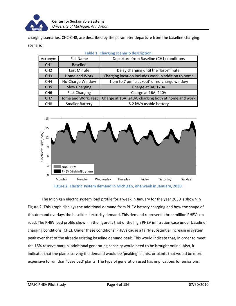
charging scenarios, CH2‐CH8, are described by the parameter departure from the baseline charging
scenario.
Table 1. Charging scenario description
Acronym Full Name Departure from Baseline (CH1) conditions
CH1 Baseline ‐
CH2 Last Minute Delay charging until the ‘last‐minute’
CH3 Home and Work Charging location includes work in addition to home
CH4 No‐Charge Window 1 pm to 7 pm ‘blackout’ or no‐charge window
CH5 Slow Charging Charge at 8A, 120V
CH6 Fast Charging Charge at 16A, 240V
CH7 Home and Work, Fast Charge at 16A, 240V, charging both at home and work
CH8 Smaller Battery 5.2 kWh usable battery
Figure 2. Electric system demand in Michigan, one week in January, 2030.
The Michigan electric system load profile for a week in January for the year 2030 is shown in
Figure 2. This graph displays the additional demand from PHEV battery charging and how the shape of
this demand overlays the baseline electricity demand. This demand represents three million PHEVs on
road. The PHEV load profile shown in the figure is that of the high PHEV infiltration case under baseline
charging conditions (CH1). Under these conditions, PHEVs cause a fairly substantial increase in system
peak over that of the already existing baseline demand peak. This would indicate that, in order to meet
the 15% reserve margin, additional generating capacity would need to be brought online. Also, it
indicates that the plants serving the demand would be ‘peaking’ plants, or plants that would be more
expensive to run than ‘baseload’ plants. The type of generation used has implications for emissions.
Monday Tuesday Wednesday Thursday Friday Saturday Sunday0
3
6
9
12
15
18
Electrical Load [GW]
Non‐PHEV
PHEV (High Infiltration)

Center for Sustainable Systems University of Michigan, Ann Arbor
MPSC PHEV Pilot Study Page 5 of 156 07/30/2010
1.1.2 Fleet Infiltration
In addition to charging behavior, the effect of PHEVs on the grid will depend on fleet infiltration rates
and the total number of PHEVs on the road. In this study, five fleet scenarios were examined: a zero
infiltration rate (FI1), a low infiltration rate (FI2), a medium infiltration rate (FI3), a high infiltration rate
(FI4) and a maximum infiltration rate (FI5). These infiltration curves over the 2010 to 2030 time frame
are displayed in Figure 3 below. The Obama administration has set a goal of 1 million PHEVs on the road
by 2015[1]. As Michigan represents approximately 1/30 of the national population, proportionally the
state would support 33,000 PHEVs to achieve this goal. Within the inset graph of Figure 3 the dashed
marker signifies this 33,000 vehicle target. As shown, the model in this study realizes at least this many
PHEVs in the medium, high, and maximum infiltration scenarios. PHEVs have an assumed life of 10
years, and each PHEV is assumed to displace a CV in the same size class.
Figure 3. PHEV infiltration rates, 2010 ‐ 2030
Electricity usage rates and fuel economies for PHEVs and conventional vehicles (CVs) were
collected from OEM pre‐production publications, academic research and Environmental Protection
Agency (EPA) ratings. No technological improvements were assumed for the analysis of PHEVs, so
emissions reduction from gasoline displacement may be conservative. Fuel economy improvement
factors for CVs were taken from the 2009 Energy Information Agency (EIA) Annual Energy Outlook
(AEO).
2010 2012 2014 2016 2018 2020 2022 2024 2026 2028 20300
2
4
6
8
Millions of PHEV
2014 2015 2016
50,000
100,000
33,000*
Low PHEV infiltration (FI2)
Med PHEV infiltration (FI3)
High PHEV infiltration (FI4)
Max PHEV infiltration (FI5)
Total on‐road vehicles
73.3% PHEV
42.6% PHEV
13.3% PHEV
3.2% PHEV
No. ofPHEVson theroad

Center for Sustainable Systems University of Michigan, Ann Arbor
MPSC PHEV Pilot Study Page 6 of 156 07/30/2010
1.1.3 Electric Grid
Modeling the electricity sector is complicated due to its bid‐based and nodally priced real time
operation. Specific economic data, like marginal generation costs on individual generation assets in the
Michigan electric grid, was proprietary information and therefore not available. The power dispatch
methods in this study did not attempt to simulate a true economic dispatch, but rather approximated
electricity dispatch. The electricity generation capacity model simulated decisions to add new
generation to the grid or to retire existing capacity. The new generation capacity that is added
determined the yearly grid fuel mix, assuring that renewable portfolio standard (RPS) and marginal
spinning reserve requirements were met. Once decisions to retire existing or add new generation
capacity were made, MEFEM dispatched generation assets to meet this electricity demand.
The electric power capacity factor dispatch model utilized four future grid scenarios that
specified the fuel types of capacity additions made in the model over the 20 year time frame. These
electric grid scenarios, EG1 through EG4, vary in the amount of renewable generation added, the
amount of nuclear capacity added and the number of retirements to existing generation assets. A
simplified economic dispatch algorithm was also explored in this study. In this economic dispatch model,
additional scenarios were which that include variations in GHG costs. The capacity factor dispatch
model, uses historical power plant performance data from EPA’s Emissions & Generation Resource
Integrated Database (eGRID) to simulate future power plant operation. The economic dispatch model,
dispatches generating assets based on fuel cost predictions and plant heat rates.
Figure 4 below shows the steps for electricity dispatch by using a load duration curve. The curve
marked #1 is the total system electric demand (PHEV and non‐PHEV load). In both dispatch methods,
wind power is first applied to the total system demand as a negative load. This step is illustrated by the
curve marked #2 in Figure 4 below. Simulated wind farm power outputs for multiple sites in Michigan
were used (NREL wind integration database) to compile an ‘average’ wind load for Michigan. Next,
hydro electric generation is applied to the system load in a ‘peak‐shaving’ operation shown as curve #3
in Figure 4. The increase in the lower demand levels from curve #2 to curve #3 represent the Ludington
pumped hydro storage plant. All other generating assets are then dispatched to meet the remaining
demand via the Capacity Factor Dispatch or Economic Dispatch method.

Center for Sustainable Systems University of Michigan, Ann Arbor
MPSC PHEV Pilot Study Page 7 of 156 07/30/2010
Figure 4. Load duration curve showing hydro and wind dispatch.
The evolution of Michigan’s electricity supply system will be shaped by many factors including
environmental regulations, generation technologies, regional demand, and economic conditions. Four
scenarios were developed to simulate future pathways of the Michigan grid. In addition to the base case
generation scenario options include high renewable, high nuclear, and a combination of both.
1.2 Key Findings & Conclusions
This study found that any level of PHEV infiltration will decrease greenhouse gas (GHG) emission
in all the simulations analyzed. This reduction in total statewide system greenhouse gases from
electricity and transportation, under the baseline charging and electricity grid mix, ranged from 0.4 to
11.0 billion kgCO2e (GHGs) in 2030, a 0.4% to 10.7% reduction, depending on the infiltration level, as
seen in Figure 5.
Over the course of the 20 year timeframe, infiltration of PHEVs reduces total GHG emissions by
3 to 58 billion kgCO2e. GHG emissions of a PHEV, per mile driven, range from 275 to 240 gCO2e per mile
in 2030 depending upon the allocation method and the infiltration scenario used. Gasoline consumption
is reduced, as is expected from PHEVs.

Center for Sustainable Systems University of Michigan, Ann Arbor
MPSC PHEV Pilot Study Page 8 of 156 07/30/2010
Figure 5. Total GHG emissions (transportation and electricity) for the year 2030 for all infiltration scenarios (EG1, CH1)
Due to the decrease in gasoline consumption, PHEVs were found to reduce total system criteria
pollutant emissions of CO, NOX and VOC. Gasoline did not have associated lead emissions, so an increase
in electricity generation always resulted in an increase of lead. This is a limitation of the dataset used for
gasoline emissions, as it does not include values for lead emissions. While this is omission is reasonable
for the combustion of gasoline, the upstream processes for processing gasoline should include electricity
and thus some lead emissions. Conversely, the emissions data used for electricity generation did not
differentiate between particulate matters, PM10 and PM2.5. For electricity generation, the assumption
was made that all particulate matter was tracked as PM10; therefore, a decrease in gasoline always
resulted in a decrease in PM2.5 emission levels as the gasoline dataset properly differentiated the two
emissions. Although lead and PM2.5 emissions are reported, the reader should remember that data is
missing either for the transportation or electricity sector. In each infiltration scenario, total system
emissions of SOX increased because of the additional electricity demands from PHEV battery recharging.
The especially high SOX is largely due to the fuels consumed for electricity generation versus gasoline,
but the results may be inflated because the dispatch model used in this study did not take sulfur caps
into account. A graph displaying these changes in total system criteria air pollutants is shown in Figure
53 for the baseline charging and grid scenarios. While some pollutant emissions did increase, these are
local emissions at a limited number of power plants. Removing older plants and increasing new
Zero Low Med High Max0
2
4
6
8
10
12x 10
10
Infiltration Scenario
kg GHG, Electricity and Transportation sectors
Total GHG emissions in 2030 for fleet scenarios, (Base grid/charging)
Electricity Upstream
Electricity Generation
PHEV Gasoline Upstream
PHEV Gasoline Combustion
CV Gasoline Upstream
CV Gasoline Combustion

Center for Sustainable Systems University of Michigan, Ann Arbor
MPSC PHEV Pilot Study Page 9 of 156 07/30/2010
generation with high renewable decreases all criteria air pollutants compared to a baseline grid
scenario, but SOX emissions still increase with PHEV infiltration.
Figure 6. Change in total system emissions between FI1 and FI4 (EG1, CH1, 2030)
Total fuel cycle energy, or well‐to‐wheels energy use for PHEVs, under the baseline charging and
electric grid mix scenarios was lower than that of the average per mile rate of the CV fleet. By
consuming gasoline, a vehicle with a fuel economy of 30 miles per gallon, the average for the 2030 CV
fleet, 5.2 MJ are consumed per mile accounting for upstream and combustion energy consumption for
gasoline. Depending on the allocation method, for the CH1 scenario on road PHEVs consumption
ranged from 3.8 to 4.2 MJ per mile in the base grid scenario. Since the per mile total fuel cycle
consumption is lower for PHEVs, increasing the number of PHEVs in the fleet reduces the total
transportation sector energy use.
Figure 7. Percentage of travel driven electrically by charging scenario
Within the different charging scenarios, the greatest decreases in greenhouse gas emissions and
CO Pb NOx PM2.5 PM10 VOC SOx‐25
‐20
‐15
‐10
‐5
0
5
10
Percent Chan
ge from FI1
Home Last Min. H & W Window Slow Fast Fast H & W 1/2 Batt.0
20
40
60
80
100
Charging Scenario
Percent of Miles Driven [%]
Electric
Gasol ine
Center for Sustainable Systems University of Michigan, Ann Arbor
MPSC PHEV Pilot Study Page 10 of 156 07/30/2010
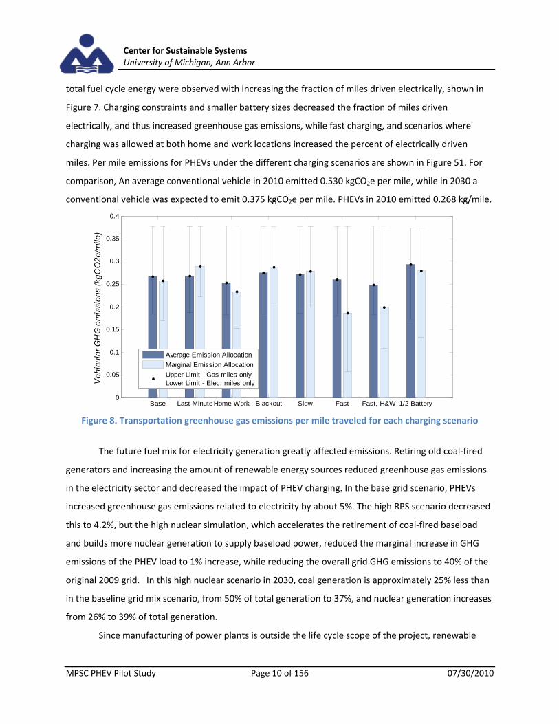
total fuel cycle energy were observed with increasing the fraction of miles driven electrically, shown in
Figure 7. Charging constraints and smaller battery sizes decreased the fraction of miles driven
electrically, and thus increased greenhouse gas emissions, while fast charging, and scenarios where
charging was allowed at both home and work locations increased the percent of electrically driven
miles. Per mile emissions for PHEVs under the different charging scenarios are shown in Figure 51. For
comparison, An average conventional vehicle in 2010 emitted 0.530 kgCO2e per mile, while in 2030 a
conventional vehicle was expected to emit 0.375 kgCO2e per mile. PHEVs in 2010 emitted 0.268 kg/mile.
Figure 8. Transportation greenhouse gas emissions per mile traveled for each charging scenario
The future fuel mix for electricity generation greatly affected emissions. Retiring old coal‐fired
generators and increasing the amount of renewable energy sources reduced greenhouse gas emissions
in the electricity sector and decreased the impact of PHEV charging. In the base grid scenario, PHEVs
increased greenhouse gas emissions related to electricity by about 5%. The high RPS scenario decreased
this to 4.2%, but the high nuclear simulation, which accelerates the retirement of coal‐fired baseload
and builds more nuclear generation to supply baseload power, reduced the marginal increase in GHG
emissions of the PHEV load to 1% increase, while reducing the overall grid GHG emissions to 40% of the
original 2009 grid. In this high nuclear scenario in 2030, coal generation is approximately 25% less than
in the baseline grid mix scenario, from 50% of total generation to 37%, and nuclear generation increases
from 26% to 39% of total generation.
Since manufacturing of power plants is outside the life cycle scope of the project, renewable
Base Last Minute Home-Work Blackout Slow Fast Fast, H&W 1/2 Battery0
0.05
0.1
0.15
0.2
0.25
0.3
0.35
0.4
Ve
hicu
lar
GH
G e
mis
sion
s (k
gCO
2e
/mile
)
Average Emission Allocation
Marginal Emission Allocation
Upper Limit - Gas miles onlyLower Limit - Elec. miles only

Center for Sustainable Systems University of Michigan, Ann Arbor
MPSC PHEV Pilot Study Page 11 of 156 07/30/2010
generation has no associated total fuel cycle energy. Increasing the amount of renewable generation in
the system has a significant impact on the total fuel cycle energy. By retiring coal plants and increasing
nuclear and natural gas generation, the high nuclear scenario had a greater effect on emissions than the
high RPS scenario. However, PHEVs within the high RPS scenario had the lowest per mile energy
consumption, at 3.5 MJ/mile using a marginal allocation method, while the high nuclear scenario
increased PHEV per mile energy use to above the base scenario rates. For all the grid scenarios, per mile
PHEV energy use was still lower than CV energy use.
1.3 Recommendations and Future Work The results of this study imply that PHEV adoption should be encouraged within the state because in
every scenario extrapolating a future Michigan grid, increasing the infiltration of PHEVs decreased
greenhouse gases, transportation energy, and most criteria pollutants. Increasing PHEVs also reduced
the state’s petroleum use.
The examination of the charging scenarios indicate that in order to avoid creating new peaks in
electricity demand, more charging locations and last minute charging are the best strategies. Fast
charging would force new, cleaner generation into the grid; however, this would come about by creating
new peaks in the system electrical demand that, in this model, creates the need for new cleaner
generating capacity. Home and work charging provides a similar electric‐to‐gasoline miles ratio as fast
charging, and home and work charging produces similar reductions in GHG emissions to fast charging
without creating such large peaks in demand using the average allocation method. If the goal is to avoid
creating large peaks while still increasing total electric miles driven, then investments in work charge
infrastructure will work better than investments in fast charge infrastructure.
Within the model new generating assets are assumed to be state of the art, and much of
Michigan’s power is supplied by an aging coal fleet. To bring about the greatest environmental
improvements, older coal‐fired power plants should be retired and replaced with cleaner generating
sources. When the grid was improved, the additional emissions attributed to PHEVs were also reduced.
One of the greatest difficulties encountered in developing the methodology for the report was
assigning emissions from electricity to the PHEVs. While not a policy recommendation, a standardized
methodology for assigning electricity generation emissions due to PHEV charging is needed to
definitively quantify the environmental effects of PHEVs. Standard allocation methodology between
surveys would facilitate comparison among research studies.

Center for Sustainable Systems University of Michigan, Ann Arbor
MPSC PHEV Pilot Study Page 12 of 156 07/30/2010
2. Introduction
In 2008, the Michigan Public Service Commission (MPSC) awarded a grant to research the proposed
Plug‐in Hybrid Electric Vehicle (PHEV) Pilot Project. This research is a collaborative effort between the
University of Michigan, Detroit Edison Energy and General Motors. The goals of the project are to
investigate the capability of PHEVs within Michigan as an economic development catalyst, determine
the vehicle‐electric utility interface in the near, mid‐ and long‐term, and understand the regional
environmental and electric utility system impacts of PHEVs in Michigan. This report outlines the
methodology, findings and recommendations of the research addressing Subtask 4.1 of the project
proposal, an analysis of environmental impacts of PHEVs in Michigan.
While this report is focused on effects within Michigan, several related studies have been
conducted to examine the environmental consequences of PHEV adoption, and a brief overview of these
studies is provided.
Two MATLAB® based models were created to analyze the environmental impacts associated
with PHEV adoption in Michigan. The structure and application of this model is detailed in this
document. Simulation results employing a variety of scenario combinations are presented. Finally, the
implications of those results are discussed, and recommendations are offered toward both future
research goals as well as policy initiatives to reduce the environmental impacts of light duty vehicles in
Michigan.
2.1 Previous Research and Context
Interest in alternatively fueled vehicles such as hybrids, plug‐in electric vehicles, and fuel cell vehicles
has been spurred in recent years by high gasoline prices and renewed concerned for national energy
independence and the environmental impacts of the transportation sector. Several earlier studies were
examined to aid the development of the methodology utilized for the evaluation of environmental
impacts of PHEVs. An abbreviated review of current literature is presented to orient the reader on the
current state of research into PHEV environmental evaluation and to show the need for this project’s in‐
depth charging, infiltration, and electricity dispatch models.
In 2008, a group at MIT[2] conducted a broad investigation into alternatively fueled vehicle
trends through the year 2035. While the group dismissed many new technologies as too expensive,
especially when compared to established gasoline vehicle lines, concluding that investment in fuel

Center for Sustainable Systems University of Michigan, Ann Arbor
MPSC PHEV Pilot Study Page 13 of 156 07/30/2010
efficiency of conventional vehicles would reduce greenhouse gas emissions at a lower retail consumer
price, plug‐in electric vehicles were selected as the alternative fuel vehicle of choice for the near term.
PHEVs were selected as the best option because they have the same range as current vehicles and
provide reductions in emissions without the need for extensive infrastructure overhauls as would be the
case to support a large fleet of hydrogen fuel cell or pure battery electric vehicles. Kromer and
Heywood, two researchers within the MIT group put together another assessment of advanced
powertrains including battery electric vehicles, hybrid electric vehicles, and plug‐in hybrid electric
vehicles[3]. They found that electrified vehicles offer an improvement to the environment over the long
term, generating less lifecycle greenhouse gases than conventional gasoline vehicles despite higher
material production costs. However, this study promoted HEVs over PHEVs, citing that the added
financial expense of PHEVs was not justified since PHEVs did not result in a direct reduction of emissions
due to the uncertainty of grid emissions. Their study utilized three different ‘grid mixes’ to apply a factor
to PHEV electricity consumption. This uncertainty in emissions allocation was also supported by Stephan
and Sullivan in their 2008 report[4]. They found that when a PHEV was charged using electricity
generated solely by fuel oil or inefficient coal plants, greenhouse gas emissions could be as high as 440
gCO2e/mile. However, they also noted that a PHEV driving short trips and charged using clean,
renewable sources had an effective emissions rate of 0 gCO2e/mile, not accounting for upstream
renewable production emissions.
There have been many studies dedicated to evaluating the greenhouse gas emissions of plug‐in
electric vehicles. In Section 5.6, a comparison is made between the Michigan simulation results and
other published per mile emissions, showing average emissions rates ranging from 145 gCO2e/mile to
385 gCO2e/mile (For reference, Grimes‐Casey, et al. place total fuel cycle emissions for conventional
vehicles at roughly 585 gCO2e/mile)[5]. This large range in per mile emissions stems from the
methodology employed in quantifying and attributing electricity generation emissions to the
transportation sector as well as the types of electricity generating assets, used to meet vehicle electricity
demand . The Electric Power Research Institute (EPRI) Environmental Assessments of Plug‐In Hybrid
Electric Vehicles[6] alone reports a range of about 150‐325 gCO2e/mile, depending solely on the carbon
intensity of the grid scenario they used. Uncertainty in resulting criteria air pollutants emissions is
similarly associated with the fuels used to produce electricity.
Three methodologies for determining electricity emissions have emerged in the literature. The
simplest solution is to assume that all PHEV charging energy is sourced from one fuel type. Kromer and

Center for Sustainable Systems University of Michigan, Ann Arbor
MPSC PHEV Pilot Study Page 14 of 156 07/30/2010
Heywood as well as Stephen and Sullivan used this method in their analyses. They assumed the grid was
fueled from a single generation technology type and examined the variation in emissions from a single
PHEV, applying this resulting range of emissions to future PHEVs anywhere within the country. This can
be a good way to develop regional emissions rates if, within a specific region, the specific power plant
fuel type that will be used to charge PHEV is known. In ‘Environmental Benefits of Plug‐in Hybrid Electric
Vehicles: the Case of Alberta,’ University of Calgary researchers looked at using PHEV charging loads to
absorb nightly wind generation, resulting in a zero emissions rate[7].
A slightly more in depth solution to emissions allocations would be applying an average grid
emissions factor to the energy consumed by PHEV. Samaras’ lifecycle analysis for PHEVs applies a
national grid average to PHEV energy consumption. Again, this can be regionalized if the target grid is
known. In 2007, a Minnesota task force[8] concluded that a PHEV fleet would increase emissions
compared to an HEV fleet due to the high proportion of coal generation in the state. The report used an
average emissions factor that was based on an 80% coal, 20% wind grid to estimate the actual emissions
in the fleet. Note that, as mentioned in Samaras’ lifecycle study[9], this method considers PHEV charging
part of the total load rather than a marginal load to be met by additional generation. This distinction is
explained in greater detail in Subsection 3.5.3. A report by the University of California, Davis’ Institute of
Transportation Studies[10] explored the interaction of PHEVs with the California grid, finding that the
additional load from off‐peak PHEVs would be met by relatively inefficient natural gas generators, and
compiled both marginal and average emissions rates at hourly intervals. Assigning these additional
emissions to PHEV yields a reduction over conventional vehicles about (200 gCO2e/mile), but if the
charging is conducted as load leveling (restricted to certain hours of the night) rather than simply off‐
peak (but still allowed to charge throughout the day, away from peak times), the result is slightly lower
due to the difference in fuel mix expected to serve that additional load. However, in either charging
scenario, the result is a higher electricity emissions rate than the roughly 80%(NGCC)/20% (renewable
generation) mix used to develop California’s Low Carbon Fuel Standard.
Some reports attempt to model the grid to investigate the effect of PHEV infiltration on power
plant dispatch and new capacity additions. While the EPRI report examined PHEV infiltration at the
national level, it utilized the Energy Information Agency’s National Electricity Modeling System (NEMS)
to calculate electricity supply, demand, and prices nationwide and the National Electric System
Simulation Integrated Evaluator to simulate the addition of new electricity generating capacity and the
retirement of older assets. Other studies have modeled regional grids by assuming some fuel types will
Center for Sustainable Systems University of Michigan, Ann Arbor
MPSC PHEV Pilot Study Page 15 of 156 07/30/2010
be utilized to meet demand first, such as renewable and nuclear sources, while typically more expensive
fuel sources would only be utilized when demand is high. Kinter‐Meyer, Schneider, and Pratt at the
Pacific National Lab[11] looked at PHEVs on a regional level, ‘stacking’ generating assets by fuel type,
and estimating the number of PHEVs that could be charged using the region’s available capacity. While
the study found that greenhouse gases in each region dropped, PHEVs could lead to either an increase
or decrease in criteria pollutants depending on the mix and extent of use of generating assets in each
region. Using a similar methodology within the PJM ISO, which includes Pennsylvania, New Jersey,
Delaware, and Maryland, a study by Thompson, Webber, and Allen[12] analyzed a baseload mix of coal
and nuclear generation similar to Michigan’s grid. The historical plant output levels were ‘stacked’, and
any remaining capacity left undispatched (the ‘valley’ in the load) was allocated to PHEV load. The
amount of charging within this valley determined the number of miles that PHEVs could theoretically
travel in the PJM, which allowed determination of displaced gasoline. Greenhouse gas emissions were
reduced, but ozone and SOX emissions increased in some localities due to the restricted ‘valley‐filling’
charging times, which caused the use of more coal generated electricity. Sivaraman[13] used a similar
stacking method, but plant stacking was done by according to capacity factor rather than fuel type.
Capacity factor is a historical indicator of how often a plant is used. Plant capacity factor often correlates
to plant fuel type but treats plants separately. This report uses a dispatch method similar to Sivaraman
plant stacking, outlined in subsection 3.4.
When using an average or single source emissions factor, only the amount of charging is
necessary to calculate the resultant emissions. However, for more detailed studies modeling the grid
response to demand, the emissions due to PHEV charging depends not only on the amount of power
being pulled from the grid, but also the timing. Mentioned briefly, Kinter‐Meyer, Schneider, and
Pratt[11] and Thompson, Webber, and Allen[12] both assumed charging fell into a ‘valley‐filling’ pattern,
or that PHEV owners charged during periods of low system demand, and subsequently drove enough
that the charging filled the low system ‘valley’ periods to capacity. In the EPRI report PHEV charging was
more driver‐focused, employing a symmetric PHEV load pattern for an aggregate fleet that places about
75% of charging during off‐peak, night hours, between 10pm and 6am. However, the study notes that
this is just one possible scenario developed by heuristic driver assumptions such as primary home
charging and incentivized off‐peak charging. None of the models described utilized actual driver
behavior to describe the time of charging, which may have a significant impact on the generating assets
dispatched to meet PHEV electrical demand, and thus affect the emissions outcomes of the vehicles. The
Center for Sustainable Systems University of Michigan, Ann Arbor
MPSC PHEV Pilot Study Page 16 of 156 07/30/2010
PECM model was designed to determine time of charging from actual driver behavior (Subsection 3.1).
Many studies report that the adoption of PHEVs would increase or decrease air emissions but
this seems to vary considerably by methodologies for emissions allocation, the treatment of electricity
generation assets, the region being examined and the assumptions placed on the temporal location and
magnitude of the electric load due to electric vehicle charging. An in‐depth analysis examining PHEV
infiltration level, with a more sophisticated PHEV charging model and a specific electricity generation
mix tailored for Michigan has yet to be completed and can provide a more complete understanding of
impacts to the region and how similar methodologies might be applied to other regions to inform policy
development.
2.2 Research Objectives
This study analyzes the potential impact that PHEVs will have on the environment and includes the
following two main objectives:
1. Understand the impact of widespread PHEV adoption on full fuel‐cycle greenhouse gas
(GHG) emissions from a Michigan light‐duty vehicle fleet perspective.
2. Model the impact of a high level of PHEV adoption on air pollutant emissions in Michigan.
Overall emissions, both greenhouse gases and criteria air pollutants, will depend on the level of
PHEV infiltration within the fleet, time of charging, and changes to the electricity generation mix over
time. The model, to be discussed in later sections, also examines changes in non‐renewable and
renewable energy resource utilization as a consequence of PHEV adoption, tracking petroleum
displacement, total fossil fuel cycle energy consumption, and renewable energy use from wind, water,
biomass, and other sources.
The results of the study are intended to inform the MPSC about the potential environmental
benefits and consequences of PHEVs and the impacts of bringing on new electricity generation assets
and regulating dispatch decisions to meet increased electricity demand from PHEV charging.
Figure 9 describes the organization of the PHEV Pilot Project and highlights the relative position
of this study within the overarching pilot structure.

Center for Sustainable Systems University of Michigan, Ann Arbor
MPSC PHEV Pilot Study Page 17 of 156 07/30/2010
Figure 9. Project organization diagram of MPSC PHEV pilot project
2.3 Scope and System Definition
The geographic boundary of this study is the state of Michigan, and the vehicle fleet and power
generation initial conditions for the model are based on Michigan‐specific data. Predictions, such as
population changes or vehicle fleet growth, are also based on Michigan‐specific data. Emissions from
imported power sources and upstream processes, which occur out of state, but can be attributed to
Michigan consumption, are also tracked. The timeframe for the analysis spans 20 years, from 2010 to
2030, with the first year, 2009, developed based on current data without PHEVs or new power plants. A
longer timeframe was not investigated to reduce greater uncertainties in projections and results. Each
year is simulated with 364 days in order to have a year length of exactly 52 weeks, which simplifies
analysis.

Center for Sustainable Systems University of Michigan, Ann Arbor
MPSC PHEV Pilot Study Page 18 of 156 07/30/2010
Figure 10. High level schematic of overall system structure
Figure 10 shows the system model as an overview of the information and energy flows within
the system. The PHEV Energy Consumption Model (PECM) was built to simulate the energy
consumption of a single PHEV. The output of PECM is used by the Michigan Electricity, Fleet and
Emissions Model (MEFEM) to simulate the electric demand of a large group of PHEVs in hourly
resolution. MEFEM was designed to simulate the potential interactions and effects that an increasing
number of on‐road PHEVs would have on overall vehicle fleet emissions, including the interaction of
additional electricity demand with the electricity dispatch system and generating assets in the state of
Michigan. Scenarios that varied the infiltration levels of PHEVs, the types of new generating assets, the
method of electricity dispatch, and the charging behaviors of drivers were simulated, the results
presented and the implications discussed within this report.

Center for Sustainable Systems University of Michigan, Ann Arbor
MPSC PHEV Pilot Study Page 19 of 156 07/30/2010
2.4 Report Organization
This report is organized as follows: Section 2 described the related literature and context for the
present research and defined the objectives, purpose and system structure of the study. Section 3
discusses the modeling method in detail. Section 4 defines and documents the scenarios examined to
provide context for the results. Section 5 contains the results of the simulations and discusses their
implications. Section 6 concludes the main body of the report with a discussion of key findings and
policy implications and suggestions for further research in the discipline.

Center for Sustainable Systems University of Michigan, Ann Arbor
MPSC PHEV Pilot Study Page 20 of 156 07/30/2010
3. Methodology
This section provides a description of the MEFEM and PECM models developed for this analysis. The
desired outputs of the combined model are energy use and greenhouse gas and criteria pollutant
emissions from vehicle use and electricity generation. Figure 10, on page 18, is a schematic of data and
information flow within the model. The model is based on many publically available datasets,
represented as hexagonal inputs on the diagram, which feed into their designated simulation modules
and are either fed back as additional inputs to complementary systems or serve as components in the
output emission calculations. The roles and details of the major system modules are discussed in the
subsections below. Within the methodology section, subsection 3.1 focuses on PECM, while subsections
3.2 through 3.4 are devoted to MEFEM. Subsection 3.5 discusses the assumptions for emissions and
energy metrics and how these are allocated to PHEVs.
3.1 PHEV Energy Consumption Model
The PHEV Energy Consumption Model (PECM) is used to determine fleet average electricity and gasoline
use normalized to a single vehicle. This model uses trip data from the 2009 National Household Travel
Survey (NHTS)[14] to generate the daily profiles for vehicle charging and total gasoline use. Results are
generated for seven vehicle size classes under specified charging constraints. These results can then be
scaled by the number of PHEVs in each class in the Michigan light duty vehicle fleet to obtain aggregate
PHEV fleet consumption.
3.1.1 PHEV Characterization
In PECM, PHEVs are assumed to be in one of four operation states at all times: Parked and not charging,
parked and charging, driving in charge depletion mode, and driving in charge sustaining mode. To
describe a PHEV’s operation in each of these states, they are characterized by their battery size, the
average rate that they consume electricity on the road, and their average liquid fuel economy. Battery
size is measured in kWh and has a default value of 10.4 kWh of usable energy for all vehicle types. 10.4
kWh represents a 16 kWh battery being utilized for 65% of its SOC range, which would approximate a 40
mile range in a midsize vehicle. Consumption characteristics are assigned based on average values for
vehicle size classes and are given in Table 2. PECM examines PHEVs in seven size classes, corresponding
to the EPA’s light duty vehicle classifications. These include subcompact, compact, midsize car, large

Center for Sustainable Systems University of Michigan, Ann Arbor
MPSC PHEV Pilot Study Page 21 of 156 07/30/2010
car, van, SUV, and pickup. Each class has associated average electricity and fuel consumption values
taken from academic, OEM publications, and EPA fuel economy statistics[15]. Please see Appendix F for
a comprehensive discussion on defining the vehicle characteristics.
Table 2. PHEV consumption parameters
Size Class Electricity Consumption Fuel Economy
(kWh/mi) (mpg)
Subcompact 0.240 50
Compact 0.246 43.5
Midsize Car 0.274 32.8
Large Car 0.3 26
Van 0.346 26.14
SUV 0.330 26.14
Pickup 0.372 21
3.1.2 The National Household Travel Survey
The 2009 National Household Travel Survey[14] is the primary source of information used to
determine driving behavior for PHEV users in PECM. Survey participants were asked to keep a log of
information about their daily trips during one day. The survey has over one million entries that include
trips by walking, biking, public transit, light duty vehicles, and larger vehicles. It contains a variety of
information including household demographics, when the data was collected, and information
describing each trip. The specific data that the model uses from the NHTS is the day of the week, the
vehicle class, an identifier for the vehicle driven, the start and end times of each trip, the trip distance,
the trip destination, and a weighting factor for the vehicle. The NHTS data required processing before
being entered into PECM. It was sorted such that all trips that did not pertain to light duty vehicles and
those that were missing important information or were duplicates of other vehicle trips were removed.
A household weight factor from the NHTS vehicle file was added to the NHTS trip data so that each
whicle's trip day was weighted by that vehicles use pattern. The data was then partitioned into
subgroups by vehicle class and day of the week.
The NHTS only has four classes that correspond to the seven EPA size classes identified for use in
the simulation: car, van, SUV, and pickup truck. The NHTS car vehicle class is used as the basis for the
trip behavior for the EPA classes sub‐compact, compact, midsize car, and large car in PECM. Appendix E
shows the relationship between size classes in the NHTS with their EPA counterpart. The input to PECM
from the NHTS is 28 matrices, one for each day (7) and class (4) combination, with a total of more than

Center for Sustainable Systems University of Michigan, Ann Arbor
MPSC PHEV Pilot Study Page 22 of 156 07/30/2010
700,000 vehicle trips.
3.1.3 Vehicle Trip‐days
To determine how a PHEV would be driven and charged, the model groups the trip data by vehicle.
Figure 11 shows visual depictions of a grouping of twenty nine trips by the five vehicles that took them.
The trip information in the NHTS indicates when the vehicle was on the road, how far it went, and where
it parked. Since each participant was only surveyed for one day, the assumption is made that the
vehicle’s final location at the end of the day is also the vehicle’s starting location at the beginning of the
day. Information on vehicle location and how long the vehicle will rest informs the model on whether or
not the vehicle would be charging at a particular point in time. The model takes a single day’s travel for
each vehicle and tracks the vehicle’s on road energy consumption and battery charging.
Figure 11. Vehicle trip‐day depictions of NHTS data
3.1.4 Modeling PHEV Energy Consumption
To determine the average energy consumption of a PHEV in a particular size class, the model tracks the
energy state of charge (eSOC) for each vehicle trip‐day in the NHTS for that class and day of the week. It
then aggregates all of the gasoline usage and electric power consumed for charging on a minute
resolution. These values are normalized by the weighted number of vehicles used in the aggregation.
This is performed for each day of the week, and then a weekly profile is created for that size class. The
weekly profile is repeated 52 times to get a single PHEV electricity and gasoline consumption profile for

Center for Sustainable Systems University of Michigan, Ann Arbor
MPSC PHEV Pilot Study Page 23 of 156 07/30/2010
an entire year. The model outputs unique vehicle charging profiles and annual gasoline consumptions
for each of the seven size classes.
Tracking eSOC for each vehicle in the NHTS allows approximation of the timing and energy
consumption for a vehicle undergoing the specific use pattern described by an NHTS trip‐day. Vehicles
are assumed to begin the day at 100% useable energy state of charge. When a trip is begun, electricity
is consumed at the rate specified by the vehicle size class characteristics and by the trip’s average speed.
The eSOC is calculated at the end of the trip and recorded. Equation 1 describes the slope of the vehicle
’s consumption of electricity while on a trip. is the energy state of charge of vehicle , is
the distance of the trip, is the average rate of electricity consumption of vehicle , is the size of
the usable battery, and and are the start and end times of the trip, respectively.
1 ∙ ∙ Equation 1
If the vehicle finishes the trip at a location where it is allowed to charge and it is not restricted
by any of the other charging constraints imposed by the model, it begins to charge at a rate specified at
the start of the model run. It will charge until the next trip in the trip‐day or until the vehicle’s battery is
at 100% usable state of charge. The rate of charging, , is described in Equation 2. � is the current
that vehicles charge at, � is the charge voltage, � is charging efficiency, and can be thought
of as the charging load of vehicle on the grid at time .
∙ ∙ ∙ Equation 2
Figure 12 shows the SOC profile for the trip‐day for sample vehicle 1 shown in Figure 11. In the
eSOC plot, the vehicle takes four trips and charges at 12A, 120V when it arrives at home at the end of
the day. Charging efficiency in PECM is set to 88%[11, 16]. This profile was developed using the same set
of charging constraints as the baseline charging scenario as outlined in Section 4.

Center for Sustainable Systems University of Michigan, Ann Arbor
MPSC PHEV Pilot Study Page 24 of 156 07/30/2010
Figure 12. Energy SOC plot for sample vehicle trip‐day 1
It is important to note that the fuel a vehicle consumes on the road, battery electricity or
gasoline, is determined by the vehicle’s mode of operation: charge depleting or charge sustaining. In
charge depleting mode, the vehicle consumes solely battery electricity for propulsion. This is the default
mode. Once the usable battery electricity is depleted (eSOC drops to 0% of its usable range), the vehicle
switches to the charge sustaining mode. In this mode it operates very similarly to a standard hybrid
vehicle, consuming only gasoline. The consumption of gasoline, Δ , during charge sustaining mode is
governed by Equation 3, below, where is the fuel economy of vehicle , is the distance of the
trip, is the distance of that trip that was driven on electricity before the eSOC went to zero.
Equation 3
Figure 13 shows the eSOC plot for trip pattern of sample vehicle 3 from Figure 11. It indicates
when the vehicle is operating in different modes. The PECM model assumes that all vehicles can drive in
either of the two consumption modes for any drive cycle, and ignores a blended operation or speed
limitations that may exist in some PHEVs.
12:00 AM 4:00 AM 8:00 AM 12:00 PM 4:00 PM 8:00 PM 12:00 AM0
20
40
60
80
100p y ( )
Time of Day
Usable Energy SO
C [%]
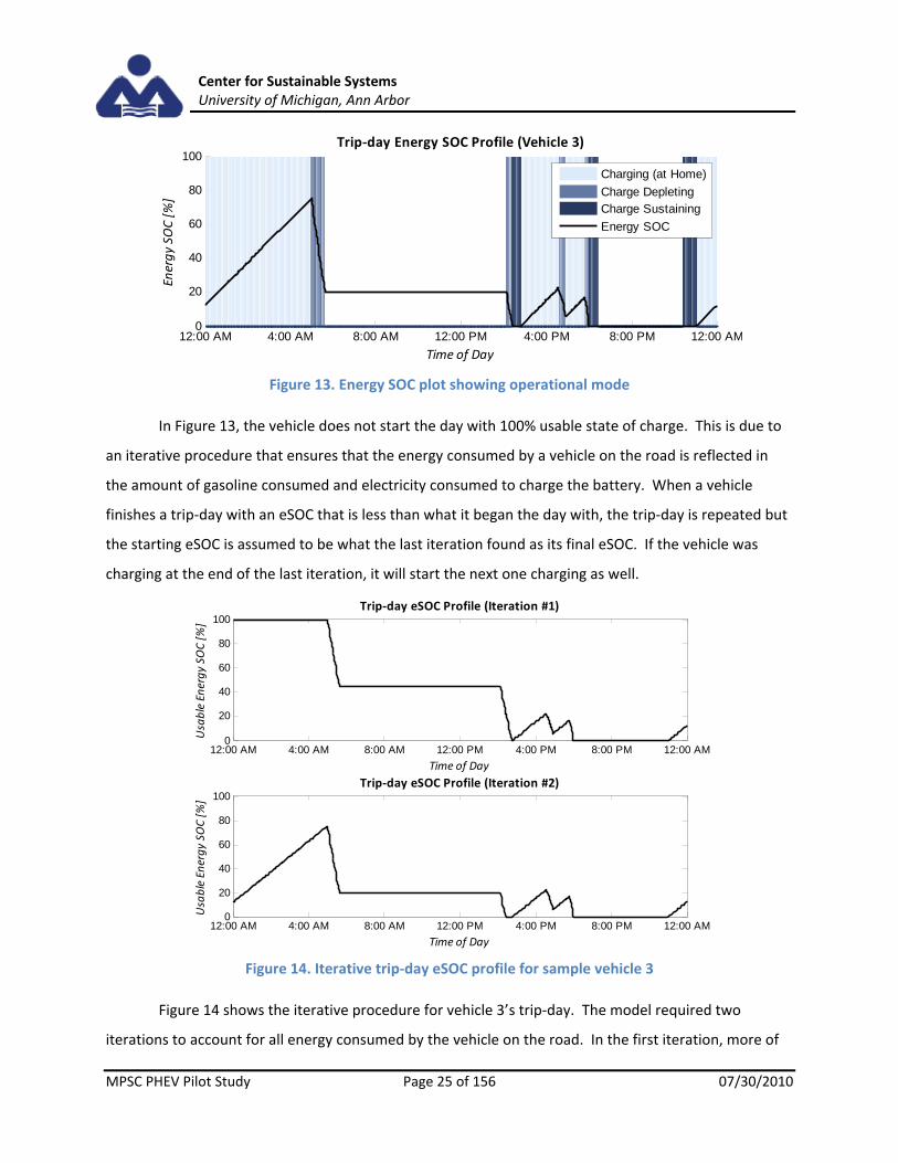
Center for Sustainable Systems University of Michigan, Ann Arbor
MPSC PHEV Pilot Study Page 25 of 156 07/30/2010
Figure 13. Energy SOC plot showing operational mode
In Figure 13, the vehicle does not start the day with 100% usable state of charge. This is due to
an iterative procedure that ensures that the energy consumed by a vehicle on the road is reflected in
the amount of gasoline consumed and electricity consumed to charge the battery. When a vehicle
finishes a trip‐day with an eSOC that is less than what it began the day with, the trip‐day is repeated but
the starting eSOC is assumed to be what the last iteration found as its final eSOC. If the vehicle was
charging at the end of the last iteration, it will start the next one charging as well.
Figure 14. Iterative trip‐day eSOC profile for sample vehicle 3
Figure 14 shows the iterative procedure for vehicle 3’s trip‐day. The model required two
iterations to account for all energy consumed by the vehicle on the road. In the first iteration, more of
12:00 AM 4:00 AM 8:00 AM 12:00 PM 4:00 PM 8:00 PM 12:00 AM0
20
40
60
80
100
Time of Day
Energy SO
C [%]
Trip‐day Energy SOC Profile (Vehicle 3)
Charging (at Home)
Charge DepletingCharge Sustaining
Energy SOC
12:00 AM 4:00 AM 8:00 AM 12:00 PM 4:00 PM 8:00 PM 12:00 AM0
20
40
60
80
100Trip‐day eSOC Profile (Iteration #1)
Time of Day
Usable Energy SO
C [%]
12:00 AM 4:00 AM 8:00 AM 12:00 PM 4:00 PM 8:00 PM 12:00 AM0
20
40
60
80
100Trip‐day eSOC Profile (Iteration #2)
Time of Day
Usable Energy SO
C [%]
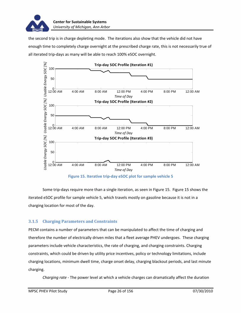
Center for Sustainable Systems University of Michigan, Ann Arbor
MPSC PHEV Pilot Study Page 26 of 156 07/30/2010
the second trip is in charge depleting mode. The iterations also show that the vehicle did not have
enough time to completely charge overnight at the prescribed charge rate, this is not necessarily true of
all iterated trip‐days as many will be able to reach 100% eSOC overnight.
Figure 15. Iterative trip‐day eSOC plot for sample vehicle 5
Some trip‐days require more than a single iteration, as seen in Figure 15. Figure 15 shows the
iterated eSOC profile for sample vehicle 5, which travels mostly on gasoline because it is not in a
charging location for most of the day.
3.1.5 Charging Parameters and Constraints
PECM contains a number of parameters that can be manipulated to affect the time of charging and
therefore the number of electrically driven miles that a fleet average PHEV undergoes. These charging
parameters include vehicle characteristics, the rate of charging, and charging constraints. Charging
constraints, which could be driven by utility price incentives, policy or technology limitations, include
charging locations, minimum dwell time, charge onset delay, charging blackout periods, and last minute
charging.
Charging rate ‐ The power level at which a vehicle charges can dramatically affect the duration
12:00 AM 4:00 AM 8:00 AM 12:00 PM 4:00 PM 8:00 PM 12:00 AM0
50
100Trip‐day SOC Profile (Iteration #1)
Time of DayUsable Energy SO
C [%]
12:00 AM 4:00 AM 8:00 AM 12:00 PM 4:00 PM 8:00 PM 12:00 AM0
50
100Trip‐day SOC Profile (Iteration #2)
Time of DayUsable Energy SO
C [%]
12:00 AM 4:00 AM 8:00 AM 12:00 PM 4:00 PM 8:00 PM 12:00 AM0
50
100Trip‐day SOC Profile (Iteration #3)
Time of DayUsable Energy SO
C [%]

Center for Sustainable Systems University of Michigan, Ann Arbor
MPSC PHEV Pilot Study Page 27 of 156 07/30/2010
and the amount of battery charging. Charging rate is defined in terms of both the voltage and current of
the charge. Voltage in the model can either be 120V or 240V, representing the two most common
residential electrical circuits permissible in the United States. The 120V circuits are limited to 12A,
which is a common wall outlet rating in the US, and the 240V circuits tend to be limited by the vehicle
software themselves[17]. The project examines three potential charging rates: 12A at 120V, 8A at 120V,
and 16A at 240V. These are based on published possible charge rates by OEMs[17].
Charging Location – This parameter defines where the vehicle is allowed to charge based on
NHTS vehicle location data. The default charging location is only at home. Home and work charging is
also examined.
Minimum Dwell time ‐ The model can also mandate a minimum dwell time in which a vehicle
must be at the charging location in order to begin charging. This represents the likelihood that a PHEV
owner will choose not to plug in their vehicle if they do not intend to stay long at their location[18].
Preliminary PECM results showed that a minimum dwell time did little to affect charging outcomes, and
minimum dwell time is not examined in depth in the study.
Charge Onset Delay ‐ A delay on the start of charging can be enforced in the model. This exists
to represent a period of time in which the vehicle may need to cool down before it is available to take a
charge[4, 6].
Charging Blackout Period ‐ The model can enforce time restrictions on vehicle charging. This is
meant to represent a limitation on charging placed on customers by utilities, or a customer’s wish to
charge off‐peak to reduce the cost of electricity. The user identifies a window of time, at an hourly
resolution, in which a PHEV owner cannot charge their vehicle.
Last Minute Charging ‐ The model can also choose to charge PHEVs at the last possible moment
such that the vehicle still receives a full charge before it leaves for a trip. This has been suggested as the
most effective way to prevent battery degradation in some lithium ion chemistries [19]and also has the
added benefit, from an electric utility’s point of view, of pushing much of vehicle charging to off‐peak
times. This implies that the vehicle owner has the ability to schedule the time of the vehicle‘s next trip,
and that vehicle software waits to charge until the ‘last minute’ while still guaranteeing full charge at the
start of the trip. If there is not enough time between trips to charge the battery fully, it charges for the
entire duration the vehicle is parked at a charging location.

Center for Sustainable Systems University of Michigan, Ann Arbor
MPSC PHEV Pilot Study Page 28 of 156 07/30/2010
3.1.6 Aggregation and Normalization
After PECM completes a vehicle trip‐day, it adds the weighted vehicle’s charging profile and gasoline
consumption to the running aggregate. Once the program has simulated all the vehicle trip‐days for a
specific day and class, it normalizes them by the weighted number of vehicles that the sample
represents. Equation 4 describes this aggregation and normalization of the charging profile (a similar
process is done for gasoline consumption), where is the aggregated and normalized hourly
charging pattern for PHEVs, is the number of vehicles in the sample, is the charging
pattern of vehicle , and is its weight factor.
∑ ∙
∑ Equation 4
Figure 16 shows the charging for each trip‐day, for each sample vehicle. Each vehicle’s charging
is assumed to be on at full power instantly, which explains the binary behavior of charging with time in
the figure. Figure 17 shows those sample trips weighted, aggregated, and normalized. Certain vehicles
have more influence on the charging pattern than others due to their weight factor. By comparing
Figure 16 and Figure 17 it can be seen that sample vehicle 4 has the most dominant charging pattern,
implying it has the largest weight factor.

Center for Sustainable Systems University of Michigan, Ann Arbor
MPSC PHEV Pilot Study Page 29 of 156 07/30/2010
Figure 16. Charging for profile for each of the sample vehicle trip‐days
Figure 17. Weighted, aggregated, and normalized charging profile for sample vehicle trip‐days
Figure 18 is an example of a weighted, aggregated and normalized charging pattern for a
Tuesday that uses the entire set of car trips from the NHTS for that day. When the sample size gets
12:00 AM 4:00 AM 8:00 AM 12:00 PM 4:00 PM 8:00 PM 12:00 AM0
0.5
11.5
Charging for Sample Vehicle 1
Time of Day
Power [kW
]
12:00 AM 4:00 AM 8:00 AM 12:00 PM 4:00 PM 8:00 PM 12:00 AM0
0.5
11.5
Charging for Sample Vehicle 2
Time of Day
Power [kW
]
12:00 AM 4:00 AM 8:00 AM 12:00 PM 4:00 PM 8:00 PM 12:00 AM0
0.51
1.5Charging for Sample Vehicle 3
Time of Day
Power [kW
]
12:00 AM 4:00 AM 8:00 AM 12:00 PM 4:00 PM 8:00 PM 12:00 AM0
0.5
11.5
Charging for Sample Vehicle 4
Time of Day
Power [kW
]
12:00 AM 4:00 AM 8:00 AM 12:00 PM 4:00 PM 8:00 PM 12:00 AM0
0.5
11.5
Charging for Sample Vehicle 5
Time of Day
Power [kW
]
12:00 AM 4:00 AM 8:00 AM 12:00 PM 4:00 PM 8:00 PM 12:00 AM0
0.2
0.4
0.6
0.8
1
1.2
1.4
Time of Day
Power [kW
]

Center for Sustainable Systems University of Michigan, Ann Arbor
MPSC PHEV Pilot Study Page 30 of 156 07/30/2010
large, the aggregate smoothes out and displays a discernable pattern for vehicle charging.
Figure 18. Normalized aggregate charging profile for a complete NHTS sample
This process of aggregation is repeated for each day of the week. The daily profiles are then
combined to create a vehicle class’ charge profile for an entire week. The model assumes that there is
no seasonal changes in driving patterns and thus replicates these weekly charging profiles over the
course of a year. The charging profiles generated by PECM do not reflect the actual charging pattern of
a single vehicle. However, they approximate the aggregate charging behavior of a light duty vehicle fleet
when multiplied by the number of vehicles in each class.
Source List
Vehicle Travel Behavior NHTS[14]
PHEV Consumption Characteristics Appendix F
Charging Efficiency Academic Publications [11, 16]
3.2 Michigan Light Duty Vehicle Fleet Modeling
After the electric and gasoline consumption parameters for individual PHEVs have been determined
these are then scaled to the greater fleet. Vehicles are tracked by size class, with different initial vehicle
sales, sales rates, infiltrations, consumption parameters, and new vehicle conventional fuel
consumptions for subcompact, compact, midsize, and large passenger car sizes, and van, SUV, and
pickup sizes. A diagram of the vehicle class mapping method can be found in Appendix E.
3.2.1 Distribution of vehicles
In this study, plug‐in vehicle infiltration is modeled as a function of sales. This approach differs from
12:00 AM 4:00 AM 8:00 AM 12:00 PM 4:00 PM 8:00 PM 12:00 AM0
0.2
0.4
0.6
0.8
1
1.2
1.4
Time of Day
Norm
alized
Charge Power [kW
h/h/veh] Daily Charge Profile ‐ Full NHTS Sample

Center for Sustainable Systems University of Michigan, Ann Arbor
MPSC PHEV Pilot Study Page 31 of 156 07/30/2010
previous studies, which simply estimate PHEV counts as a percent of on‐road vehicles. New vehicle sales
for the year 2009 were determined by comparing the number of new‐model‐year vehicle registrations in
Michigan between May 2008 and May 2009. For the years following 2009, vehicle sales were
extrapolated using regional sales data from the 2009 AEO[20]. Each year, a portion of these sales are
designated as PHEVs according to the selected infiltration scenario. Detailed information regarding
infiltration scenarios is provided in Section 4.2.
Each year the number of total vehicles, both conventional and plug‐in, is determined by two
values: population and vehicles per 1000 people. These figures, taken from the Michigan Census[21] and
Michigan motor vehicle registrations [22], are specified in Equation 5 with the symbol ‘Nall’. The
assumption is made that the number of conventional vehicles is the number of total vehicles less the
number of PHEVs (NPHEV) in that year. The conventional vehicle fleet includes conventional hybrids.
3.2.2 Conventional Vehicle Consumption
The ‘business as usual’ total gasoline usage by internal combustion vehicles was determined through
application of a ‘stock miles per gallon,’ (Fstock). This represents the average fuel consumption parameter
for all on‐road conventional vehicles. For the year 2009, this number is determined by examining total
gasoline consumption in Michigan, a value which was extrapolated from gasoline tax receipts and
vehicle miles traveled from traffic volume trends. Both datasets are part of the Federal Highway
Statistics series[23]. For years beyond 2009, an improvement factor is applied, which mimics the
removal of older, less efficient vehicles and the introduction of newer, more fuel efficient vehicles
(including conventional hybrids). This yearly improvement factor (I) is based on the improvement of the
‘stock mpg’ as reported in the AEO[20], but with an initial fuel economy that better reflects the
Michigan population. Miles driven per vehicle in the simulation is a result of PECM, abbreviated as (M).
Since PHEV purchases replace new conventional vehicle purchases, the amount of avoided
gasoline cannot be determined from this stock mpg, as the new vehicles are more efficient than the
average fleet. Therefore, the amount of gasoline that would have been consumed in a year, at year ‘y’
called ‘avoided gasoline’ or ΔG, is determined by multiplying the number of PHEVs by the projected new
vehicle fuel consumption from the AEO[20] for each size class (Fnew). Note that PHEVs are assumed to
retire after 10 years in the vehicle fleet; therefore the total avoided gasoline is for all the PHEV sold in
the current year as well as the previous ten years. The number of PHEVs sold as well as the new vehicle
fuel economies are individually calculated for each size class.

Center for Sustainable Systems University of Michigan, Ann Arbor
MPSC PHEV Pilot Study Page 32 of 156 07/30/2010
Gas consumption for on‐road conventional vehicles (GCV) for a year, ‘y’, is determined by
subtracting the avoided gasoline (ΔG) from the total gasoline consumption (GBAU) as shown in the
following equation:
∆
∆
Equation 5
3.2.3 Plug‐in Vehicle Consumption
PECM outputs the annual gasoline consumption and a normalized charging demand curve for each
vehicle size class. Both of these parameters are then scaled by the number of PHEVs in each size class.
The net PHEV electric demand is then increased by 1.09 for transmission and distribution losses [24] and
then added to the base electric demand.
Source List
Initial vehicle sales MI motor vehicle registrations [22]
New Vehicle sales rates AEO 2009 [20]
Yearly Population MI Census [21]
Vehicles per 1000 people MI motor vehicle registrations [22] , MI Census [21]
Initial total gasoline consumption Federal Highway Statistics [23]
Initial total vehicle miles traveled Federal Highway Statistics [23]
Stock improvement AEO 2009 [20]
New Vehicle fuel consumptions AEO 2009 [20]
3.3 Electricity Generation Capacity Changes
Electricity generation capacity changes refer to the power plant retirements or the addition of new
plants to the MI electricity grid. In MEFEM, the initial list of generating assets, based on those reported
in the eGRID 2005 database[25], can be seen in Appendix A and changes to this generating capacity
occur at the start of each simulation year. Retirements occur first, followed by additions to meet
Renewable Portfolio Standards (RPS) and lastly, additional capacity to meet the reserve margin
requirement imposed on utilities by the Midwest Independent Service Operator (MISO) is added.
Before delving into the details of Electricity Generation Capacity Changes and Electricity

Center for Sustainable Systems University of Michigan, Ann Arbor
MPSC PHEV Pilot Study Page 33 of 156 07/30/2010
Dispatch, three important parameters that affect a power plant’s behavior must be defined and
discussed: Nameplate Capacity, Capacity Factor and Availability Factor. A power plant’s size is generally
defined as the plant’s Nameplate Capacity, referred to in equations as , , which is the maximum
instantaneous power output of the nth power plant. Theoretically, if a power plant runs at its maximum
throughout an entire year, it should provide a total electricity generation of
, ∙
Where is the length of year in hours. A power plant running at maximum for an entire year is
unlikely due to maintenance requirements and varying load levels, but does provide an upper limit
to the amount of electricity a plant can generate. Capacity Factor is the fraction of the theoretical
maximum electricity generated that was actually produced in a year, referred to in equations as
Equation 6
This is a value that varies significantly between plants, and is due to the real world economics of
power plant dispatch. In a given year, older plants that are less efficient to run will tend to have lower
capacity factors than new power plants. Plants that run on relatively expensive fuels such as natural gas
will have lower capacity factors. Plants whose power output levels are difficult to change, such as
nuclear plants and coal, will likely be used to meet baseload and thus have very high capacity factors.
The eGRID capacity factors are used as an input to MEFEM.
Finally, Availability Factor is the fraction of the year that the plant is operational. This is referred
to in equations as . Availability factor can be thought of as a practical limit to capacity factor that
ignores economics. Even if a plant would be economically inclined to run at Emax, scheduled and
unscheduled maintenance would still require the plant to shut down at times. The only exceptions are
plants with uncontrollable outputs, such as wind, because their power output cannot be relied upon due
to the varying nature of the wind, and as a result the availability of wind power is low. Availability factor
is treated as a constant throughout all power plants of the same fuel type.
3.3.1 Generating Asset Retirements
In MEFEM, a retirement refers to the scheduled partial or complete decommissioning of a particular

Center for Sustainable Systems University of Michigan, Ann Arbor
MPSC PHEV Pilot Study Page 34 of 156 07/30/2010
generating asset. The retirements are defined based on the age of each asset, as outlined in the
Capacity Need Forum’s (CNF) 21st century report [26]. The CNF makes the assumption that generating
assets will be retired at 70 years of age. In some electricity generating capacity scenarios (discussed in
subsection 4.2), MEFEM employs a more aggressive retirement schedule for coal‐fired generating
assets. In this accelerated retirement schedule, the baseline schedule from the CNF is supplemented by
a list of retirements that occur at age 60 in addition to the retirements that already occur at 70 years. A
list of the retirements for both the baseline and accelerated decommissions are found in Appendix B.
3.3.2 Generating Asset Additions to Meet Renewable Portfolio Standards
New plants are brought online for one of two purposes: to meet Renewable Portfolio Standard (RPS)
requirements or to maintain a 15% reserve capacity margin. An RPS requires that a percentage of total
annual electricity must be generated from renewable resources. MEFEM identifies four resources that
are considered renewable and satisfy RPS generation requirements: biomass‐fired, hydroelectric, wind
and landfill gas. While this is not a comprehensive list, other renewable resources, such as solar and
geothermal, are not as viable in Michigan, and thus are not explicitly included in the model. MEFEM
employs one of two RPS conditions: either based on an extended MI RPS or on California’s RPS. The
extended MI RPS begins by following the specifications of the 2008 Michigan Clean, Renewable and
Efficient Energy Act (PA 295) Part 2, Subpart A[27], which specifies renewable goals for years 2012 –
2015. It then is extended by linearly interpolating to 20% in 2025, which represents a target proposed
by Governor Granholm[28].
In order to calculate the deficit in renewable energy generation for a particular year, existing
renewable energy, in MWh, is calculated as the product of the existing renewable generating assets’
name plate capacities, their capacity factors and the hours in a year. For any given year, the deficit in
renewable energy generation to meet the RPS requirements, , is calculated from the equation:
y Equation 7
Where is the annual amount of renewable energy generation using current assets,
is the amount of total energy demand for the current year, and is the fraction of
net generated electricity to be met by renewable sources. New renewable capacity is built if is
greater than zero.
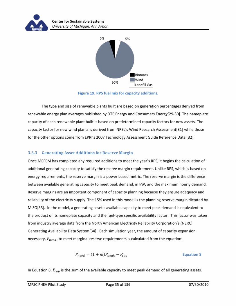
Center for Sustainable Systems University of Michigan, Ann Arbor
MPSC PHEV Pilot Study Page 35 of 156 07/30/2010
Figure 19. RPS fuel mix for capacity additions.
The type and size of renewable plants built are based on generation percentages derived from
renewable energy plan averages published by DTE Energy and Consumers Energy[29‐30]. The nameplate
capacity of each renewable plant built is based on predetermined capacity factors for new assets. The
capacity factor for new wind plants is derived from NREL’s Wind Research Assessment[31] while those
for the other options come from EPRI’s 2007 Technology Assessment Guide Reference Data [32].
3.3.3 Generating Asset Additions for Reserve Margin
Once MEFEM has completed any required additions to meet the year’s RPS, it begins the calculation of
additional generating capacity to satisfy the reserve margin requirement. Unlike RPS, which is based on
energy requirements, the reserve margin is a power based metric. The reserve margin is the difference
between available generating capacity to meet peak demand, in kW, and the maximum hourly demand.
Reserve margins are an important component of capacity planning because they ensure adequacy and
reliability of the electricity supply. The 15% used in this model is the planning reserve margin dictated by
MISO[33]. In the model, a generating asset’s available capacity to meet peak demand is equivalent to
the product of its nameplate capacity and the fuel‐type specific availability factor. This factor was taken
from industry average data from the North American Electricity Reliability Corporation’s (NERC)
Generating Availability Data System[34]. Each simulation year, the amount of capacity expansion
necessary, , to meet marginal reserve requirements is calculated from the equation:
1 Equation 8
In Equation 8, is the sum of the available capacity to meet peak demand of all generating assets.
5%
90%
5%
Biomass
Wind
Landfill Gas

Center for Sustainable Systems University of Michigan, Ann Arbor
MPSC PHEV Pilot Study Page 36 of 156 07/30/2010
Available capacity is defined as the nameplate capacity of an asset multiplied by the plant’s availability
factor. The other variables, and , are the maximum hourly electricity demand for the given year
and the reserve margin requirement (equal to 0.15)[35], respectively.
New capacity to satisfy margin is added according to a percentage mix which varies depending on the
year and the selected ‘grid mix’ scenario, discussed in subsection 4.3. This percentage mix combined
with the availability factors assigned to each fuel type is then used to determine the reserve margin
power and hence nameplate capacity to be built for each additional generating unit. This altered
generating capacity mix can now be dispatched to meet demand for the current year.
3.4 Electricity Dispatch Modeling
Once the total electric demand is quantified and all the power plants are defined, the plants must be
dispatched in order to serve this hourly load. In practice, this is a very complicated undertaking based on
physical and economic constraints. As precise economic data is proprietary information, the dispatch in
this model does not attempt to simulate a true dispatch system, but seeks to approximate electricity
dispatch in two separate ways. One method, the Capacity Factor Dispatch model, uses historical power
plant performance to forecast how power plants will be used in the future. Another method, the
Economic Dispatch model, uses cost predictions to determine which power plants will be used first. Both
of these methods have their advantages and disadvantages and both will be examined to determine the
sensitivity of PHEV electricity emissions to dispatch method.
In the model, the electric demand is managed as a point source independent of geographical
location or transmission constraints. While this lack of spatial information may introduce error into the
simulation results, the addition of new generating assets to the system makes it to difficult to accurately
model at this level of complexity.
Wind and hydroelectric plants are dispatched before all other generating assets. Their dispatch
is effectively modeled as changes to the total electricity demand. Wind assets are treated as a must‐run
and are implemented as negative demand in the model. Hydroelectric generating assets are only
operated at times of peak load and are thus dispatched as peak shavers after wind generation has been
dispatched. Pumped hydroelectric plants also increase demand in the hours of minimum demand to
account for pumping load.
After wind and hydroelectric load modifications, all remaining power plants are dispatched
based on a stacked power system. The remaining plants are ordered, or ‘stacked’, by either their

Center for Sustainable Systems University of Michigan, Ann Arbor
MPSC PHEV Pilot Study Page 37 of 156 07/30/2010
capacity factor or the cost of generation depending on the type of dispatch algorithm employed. Each
of these assets are then assigned a range of system electrical load, termed here as a power band, which
represents the required minimum levels of hourly system load under which a given plant will be
dispatched to generate electricity.
A power plant’s power band is defined with two values, , and , , where N indicates
the location of the current power plant in the dispatch order. Let DH(t) be the system electric demand
after wind and hydro, and let PN(t) be the output of the Nth power plant at any time t. PN(t) will be:
0 ,
, , ,
, , ,
Equation 9
Since there are no geographical and transmission constraints, this stacked power system
effectively keeps only one power plant running at partial output, with all other power plants either on or
off completely. “On” in this case refers to the power plant outputting , , , which is less
than the plant’s nameplate capacity. It is possible that the highest power level that the generating assets
can provide (the maximum value of , is actually below the highest level of electric demand. If
this is the case, the deficit is assumed to be met from outside the state as imported electricity. This can
be thought of as an additional power plant with its own emission factors. This system of electric dispatch
assumes that all power plants can come online instantaneously, are capable of following load perfectly,
can shut down instantaneously, and do not have any minimum output levels.
A convenient way to represent the electric demand and the effect of Equation 9 is by using a
load duration curve. In it, the electric demand profile is sorted in descending order, from highest
to lowest power demand. This will be differentiated in equations by using . In this representation
of electrical demand, chronological time has been replaced by the duration of time at which the system
is greater than the corresponding load value. The area under the curve, representing the net electrical
demand at the generating sites, is still the same. This area can be divided up into horizontal stacks which
graphically represent the power bands, thus the name “stacking” dispatch. Figure 11 shows a sample
load duration curve with three power plants for illustration purposes.

Center for Sustainable Systems University of Michigan, Ann Arbor
MPSC PHEV Pilot Study Page 38 of 156 07/30/2010
Figure 20. Load duration curve example with 3 plants
Under this method, the dispatch model can determine the power output of every power plant
for every hour in each simulated year, which will be used to determine total electrical system emissions
rate. The Capacity Factor Dispatch and Economic Dispatch models calculate the power bands differently.
Capacity Factor Dispatch requires historical capacity factors for the initial year to determine what power
bands would be needed for that year. It then scales the power bands for the changing load and asset
mix for all future years. The power plant electricity generation of the base year will be exactly equal to
its historical amount. The downside of Capacity Factor Dispatch is that by extrapolating a single year's
dispatch behavior it assumes that all of the market and fuel supply conditions inherent in historical data
are constant for the next 20 years, which is unlikely. The economic dispatch model sorts power plants by
cost of generation and dispatches them to their available capacity. While being an inaccurate predictor
of base year capacity factors, Economic Dispatch is capable of responding to changes in fuel prices and
additional emissions taxation.
The entire electricity dispatch follows these steps, illustrated in Figure 21. Let D(t) be the total
electric system demand for a year.
1. Dispatch wind assets. D(t) reduces to DW(t).
2. Dispatch hydroelectric assets and pumped hydroelectric storage assets. DW(t) changes to DH(t).
3. Determine the power bands for all remaining power plants using either Capacity Factor Dispatch
or Economic Dispatch algorithm.
4. Dispatch all remaining power plants for an entire simulation year using Equation 9 and DH(t).

Center for Sustainable Systems University of Michigan, Ann Arbor
MPSC PHEV Pilot Study Page 39 of 156 07/30/2010
Figure 21. System diagram for electricity dispatch
3.4.1 Wind Assets
Wind assets are the first generating units dispatched, and are treated as a negative load on the system.
The remaining system load is calculated as follows:
, Equation 10
Where is the total electricity demand (baseload plus additional PHEV demand plus line
losses), is the normalized wind power curve and is the remaining demand or system load
that serves as an input to the hydroelectric dispatch model. The normalized wind power curve is
analogous to capacity factor, but calculated hourly. The sum of the nameplate capacity of all the wind
assets multiplied by this curve yields the hourly power output of all the wind assets in Michigan. Wind’s
yearly capacity factor, , is calculated by integrating the normalized wind power curve and dividing
by the simulation year length, , as in Equation 11.
1 Equation 11
This is necessary for the capacity decisions model to correctly determine the amount of
renewable energy output, and allows it to build the correct amount of wind when needed. Only one
normalized wind output curve is to be used, meaning that all wind assets will have the same capacity
factor for every simulation year. Although this could mean that current existing wind farms will perform
better than expected, the only existing wind farm in Michigan as of 2005 is relatively small and thus is

Center for Sustainable Systems University of Michigan, Ann Arbor
MPSC PHEV Pilot Study Page 40 of 156 07/30/2010
not a significant source of error. The normalized wind output curve comes from the NREL Wind
Integration Datasets [31]. These were developed as part of a larger study to evaluate the impacts of
large wind infiltration. This data was based on high‐resolution simulations of the historical climate
performed by a mesoscale numerical weather prediction. In Michigan, thirteen wind farms of varying
nameplate capacity were simulated in 10‐minute intervals throughout 2004‐2006 (Figure 22).
In order to develop the normalized wind power curve, nameplate capacities of the sited wind
farms were used to normalize each power output entry. Then, all three years for all thirteen sites were
reduced to hourly resolution, and all 39 data sets (thirteen sites multiplied by three years) were then
averaged to end with a single vector of 8736 values. This is from the equations above. Since
each simulation year is only 364 days, the last two days in the 2004 data and the last day in 2005 and
2006 data will be ignored.
Figure 22. The 13 Michigan sites simulated by the NREL wind integration dataset
The resulting normalized wind output curve has a yearly capacity factor of 29.8%. Figure 23
displays two weeks of this curve; one in January and one in June. In general, winter months have higher
outputs than summer months.

Center for Sustainable Systems University of Michigan, Ann Arbor
MPSC PHEV Pilot Study Page 41 of 156 07/30/2010
Figure 23. Sample of normalized wind power generation curve (week in Jan. and June)
The integration of wind into system dispatch effectively decreases the power demand curve.
However, the variability of wind plant power output increases variability in the electric load. Figure 24
shows the effect of wind dispatch on the system electric load for four days.
Figure 24. Wind dispatch’s effect on system demand
3.4.2 Hydroelectric Assets
Like wind, water assets, such as run of river turbines and pumped storage dams are dispatched prior to
the economic or capacity factor stacking dispatch. It is assumed that hydroelectric plants would be
dispatched at times of greatest load, and are deployed to ‘shave’ the peak load. The amount of peak
shaving that occurs is based on historical monthly generation values from 2005[36], thus assuming that
the energy generated in 2005 is indicative of the energy that would be produced in subsequent years.
No water assets are retired in the simulation, and no new water assets are brought online.
After the wind output is treated as negative load, the remaining load is split into monthly load
curves, and the hydro assets are deployed separately each month. Within a month, the hours are sorted
from time of highest to lowest demand to create a monthly load duration curve, . Since each

Center for Sustainable Systems University of Michigan, Ann Arbor
MPSC PHEV Pilot Study Page 42 of 156 07/30/2010
hydroelectric plant is treated separately, a subscript is defined to represent the electric demand
that the Nth hydroelectric plant will dispatch to. would then be equal to .
The peak shaving algorithm dispatches the hydroelectric plants in two ways. First, the plant
dispatches at nameplate capacity until it reaches a duration level , named the split duration. Then, the
dispatch levels drop to zero following the shape of the demand duration curve. These two portions of
dispatch will be named the Nameplate Dispatch and the Decreasing Dispatch, respectively. Let be
the sorted hydroelectric plant output for the Nth hydroelectric power plant:
,
,
Equation 12
where , is the plant’s nameplate capacity, and is the demand at the split duration
point (a constant value). Figure 25 shows an example of the electric dispatch for an exceptionally large
hydroelectric plant using Equation 12, with the split duration occurring at about hour 75.
Figure 25. Example of the sorted dispatch shown for a very large hydroelectric plant.
From EIA form 906[36], the energy provided by each plant, , for each month is known. The
objective of the peak shaving dispatch model is to find the split duration point such that the energy
output of the plant matches :
Equation 13
represents the number of hours in a month. The algorithm finds tS by starting with a tS value
0 100 200 300 400 500 600 700 7440
1
2
Duration (hrs)
Po
wer
ou
tpu
t (G
W)

Center for Sustainable Systems University of Michigan, Ann Arbor
MPSC PHEV Pilot Study Page 43 of 156 07/30/2010
of one hour, and then increases tS by one hour until Equation 13 is met. Each hydroelectric asset is
dispatched in this same manner, effectively reducing the demand as described in Equation 14:
Equation 14
The dispatch algorithm then moves onto the next hydro plant. Figure 26 demonstrates the
effect that the example plant has on the sorted electric demand. The nameplate dispatch portion
follows the electric demand curve perfectly: at each point, the electric demand is lowered by PN,NPC. At
the split duration point, the electric demand curve now flattens out at Pmin: the electric demand curve at
the split duration point minus the plant’s nameplate capacity. The sum of the nameplate dispatch and
decreasing dispatch areas will equal EN. It is possible that the algorithm cycles through all possible split
duration points and EN is not met. The plant will run at nameplate capacity throughout the entire month,
and the excess energy that was recorded will not be used in the model. This amounts to approximately a
6% error in hydroelectric energy output between historical generation as reported by the EIA in 2005
and the output of MEFEM.
Figure 26. Effect of applying the sorted dispatch from Figure 25 to a July load.
This process is repeated for all hydroelectric plants. Then, after the last hydroelectric plant has
been dispatched, can be calculated via:

Center for Sustainable Systems University of Michigan, Ann Arbor
MPSC PHEV Pilot Study Page 44 of 156 07/30/2010
Equation 15
The load is rearranged into a chronological time arrangement, and this load is input to the
stacking dispatch function (either Capacity Factor Dispatch or Economic Dispatch) for dispatch of the
remaining generating assets. Figure 27 shows the initial sorted demand for July as the topmost sloping
line, the dispatched run of river plants as the cascading lines below the initial demand, and finally the
dispatched Ludington Pumped storage plant.
Figure 27. Sorted demand curve and hydro asset deployment
A key feature of the Michigan generation mix is the Ludington pumped storage plant,
represented by the anomalous load duration curve in Figure 27. This plant, unlike the other run of river
hydro assets, is an extremely large reservoir that empties out into Lake Michigan and pumps back up
during cheaper generation times, assumed here as the times of lowest demand in the model. For all
hours that power was delivered, the generator places additional demand in the ‘off hours’ according to
the energy consumed for pumping[36], starting from the time of lowest demand. Figure 28 shows the

Center for Sustainable Systems University of Michigan, Ann Arbor
MPSC PHEV Pilot Study Page 45 of 156 07/30/2010
new hourly load curve in bold, which has been ‘flattened’ after the hydroelectric dispatch. For the
dispatch algorithm, Ludington is treated separately, and follows the same area fit algorithm but starting
at the highest duration point and adding load instead of removing it.
Figure 28. Unsorted original and post‐hydro dispatch demand curve
3.4.3 Capacity Factor Dispatch
Capacity Factor Dispatch is based on each power plant’s capacity factor for a given year, which implies
the amount of electricity generated by that plant is known. In MEFEM, Capacity Factor Dispatch is
accomplished using each plant’s historical generation from 2005 [25] coupled with historical system
electricity demand for that year [37]. The power plant stacking order is determined by capacity factor in
descending order. The power bands calculated for 2005 are the basis for power bands in all other years,
and are sized such that the power plant’s yearly energy output exactly matches the historical amount:
, ∙ ∙ Equation 16
Where is the asset’s historical capacity factor and , is the plant’s nameplate capacity.
Equation 16 and Equation 9 form the mathematical basis for the development of the power bands. The
Capacity Factor Dispatch algorithm is written such that the size of each plant’s power band meets both
equations. An initial guess for power band size is made by:

Center for Sustainable Systems University of Michigan, Ann Arbor
MPSC PHEV Pilot Study Page 46 of 156 07/30/2010
,
0 1
, 1
,, ∙ 1
, ∙ , 1
Equation 17
In Figure 29, a portion of a load duration curve focused on the lowest point is shown. This point
is referred to as the minimum demand level. For all power plants whose upper power band limit is less
than the minimum electric demand level, the size of their power band will be exactly as predicted in
Equation 17, since they are running all year. However, for plants whose power band levels are located
above the minimum electric demand level, the electric demand level dips below their maximum for
some hours, and the plant’s net energy output will be less than required (Equation 16 is not met). Figure
29, left, shows that plant A, at the initial guess of power band, will have a deficit in energy generation.
The Capacity Factor Dispatch algorithm iteratively increases the size of the power bands, as shown in
Figure 29 (right), until Equation 16 is met for all plants in the dispatch order. The increase in the power
band shown in Figure 29 has been exaggerated for clarity.
Figure 29. (Left) Original plant stack (Right) Increased plant A power band.
This iterative process is done for all plants in the stack. After calculating the power band for the
last plant in the dispatch stacking order there remains a system energy deficit, which is assumed to be
met by imported energy from the MISO system. The percentage of imported energy is calculated only
once, in the base year 2005. It is then kept constant for all simulation years. This process is known as the
initial stack and the resulting modeled capacity factors are exactly equal to the input capacity factors.
After the initial stack and imported energy percentage calculations are complete, the Capacity
Factor Dispatch begins dispatching for all the simulation years; however, it must have a way to handle
new power plants and changes to electric demand from year to year. New assets are given an assumed
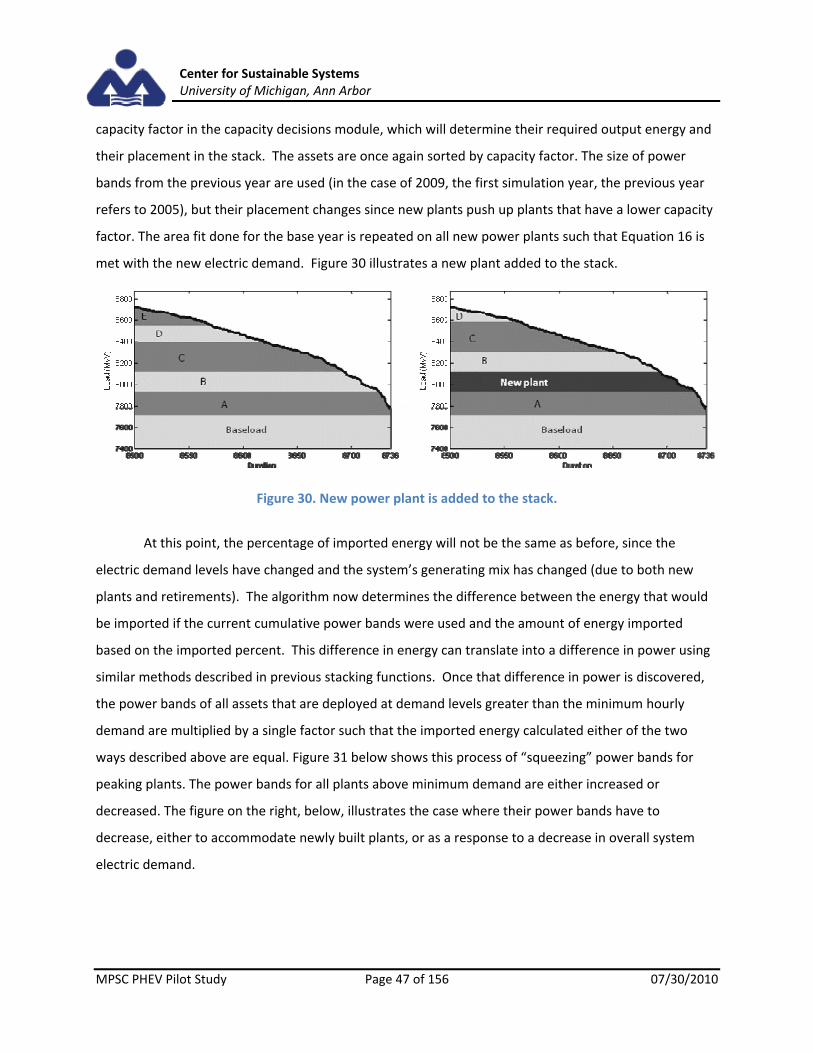
Center for Sustainable Systems University of Michigan, Ann Arbor
MPSC PHEV Pilot Study Page 47 of 156 07/30/2010
capacity factor in the capacity decisions module, which will determine their required output energy and
their placement in the stack. The assets are once again sorted by capacity factor. The size of power
bands from the previous year are used (in the case of 2009, the first simulation year, the previous year
refers to 2005), but their placement changes since new plants push up plants that have a lower capacity
factor. The area fit done for the base year is repeated on all new power plants such that Equation 16 is
met with the new electric demand. Figure 30 illustrates a new plant added to the stack.
Figure 30. New power plant is added to the stack.
At this point, the percentage of imported energy will not be the same as before, since the
electric demand levels have changed and the system’s generating mix has changed (due to both new
plants and retirements). The algorithm now determines the difference between the energy that would
be imported if the current cumulative power bands were used and the amount of energy imported
based on the imported percent. This difference in energy can translate into a difference in power using
similar methods described in previous stacking functions. Once that difference in power is discovered,
the power bands of all assets that are deployed at demand levels greater than the minimum hourly
demand are multiplied by a single factor such that the imported energy calculated either of the two
ways described above are equal. Figure 31 below shows this process of “squeezing” power bands for
peaking plants. The power bands for all plants above minimum demand are either increased or
decreased. The figure on the right, below, illustrates the case where their power bands have to
decrease, either to accommodate newly built plants, or as a response to a decrease in overall system
electric demand.

Center for Sustainable Systems University of Michigan, Ann Arbor
MPSC PHEV Pilot Study Page 48 of 156 07/30/2010
Figure 31. Changes in power bands to meet required imported energy percentage 3.4.4 Economic Dispatch
The economic dispatch algorithm creates a stacked dispatch order of generating assets based on their
cost of generation. Cost is calculated for each power plant, the power plants are sorted from cheapest
to most expensive to generate electricity, and then the power bands assigned are:
,
0 1
, 1
,, ∙ 1
, ∙ , 1
Equation 18
Where is the plant’s availability factor. No further refinement of power band size is required
(as opposed to Capacity Factor Dispatch, where the requirements for power bands were different). Cost
is calculated on a $/MWh basis. The total cost of generation is the sum of fuel cost and emissions
related costs. Fuel costs are calculated by:
Equation 19
Where is the power plants heat rate, the ratio of fuel energy consumed per electrical energy
produced; is the total cost of fuel, and and are the amounts of electricity generated
and fuel energy consumed, respectively. Carbon dioxide cost is calculated by taking eGRID specific
emission factors and applying global warming potentials from the IPCC 4th Assessment Report[38] to
methane and nitrous oxide:

Center for Sustainable Systems University of Michigan, Ann Arbor
MPSC PHEV Pilot Study Page 49 of 156 07/30/2010
25 298 Equation 20
Finally, the total generating cost is:
Equation 21
The only exception to Equation 21 is the total generating cost of nuclear power plants. These
costs are assumed to remain constant throughout the simulation and include operation and
maintenance. All renewable plants are assumed to have no cost, thereby ensuring they are always
dispatched. Units for cost are in $2008/MWh generated.
Source List
Heat Rates EPA eGRID 2005 [25]
Emission Factors EPA eGRID 2005 [25]
Fuel Costs EIA Annual Energy Outook 2010 [39]
CO2 Costs American Clean Energy and Security Act of 2009 ‐ H.R. 2454 [40]
3.5 Emissions & Life Cycle Metrics
The outputs of MEFEM are life cycle emissions and energy use for both vehicle liquid fuel consumption
and electricity generation. The model tracks criteria pollutants: CO, NOX, Pb, PM2.5, PM10, SOX and VOCs,
and greenhouse gases: CO2, CH4, and N2O. It aggregates GHGs using the most recent Global Warming
Potentials[38] identified by the IPCC. It also tracks total fuel cycle energy for stationary and mobile
energy generation sources. MEFEM applies emissions factors (kg/kWh of electricity or kg/gal of fuel) or a
upstream energy factor (MJ/mmBtu of fuel input for electricity or MJ/gal of fuel) to the energy produced
from each power plant and its heat rate or to the gallons of gasoline consumed to determine the total
fuel cycle energy usage and emissions. Emissions factors are separated into both their upstream and
combustion components so that they may be tracked separately.
3.5.1 Electricity Generation Energy and Emissions
The electricity system’s total fuel cycle is described in Figure 32, where ‘m’ denotes atmospheric
emissions and ‘E’ denotes energy flow. EUser refers to the site energy for electricity, consumer’s actual
meter reading. A constant transmission and distribution loss factor is applied of 1.09 ([24]), and this is

Center for Sustainable Systems University of Michigan, Ann Arbor
MPSC PHEV Pilot Study Page 50 of 156 07/30/2010
treated as the electricity that power plants must generate, from subsection 3.4. Note that
manufacturing of plants is not included in this accounting.
Figure 32. Total fuel cycle diagram for electricity production.
Emissions Factors
The total emissions from electricity generation are comprised of both combustion emissions and
upstream emissions, as denoted in Figure 32. Combustion refers to the emissions released when the fuel
is burned, while upstream refers to the emissions released while mining, drilling, refining the fuel, and
transportation of the fuel from the extraction site to point of combustion. Upstream emissions factors
for electricity are from the USLCI database [41] examined using the SimaPro software. Each of the
eleven emissions types were determined in SimaPro by subtracting the “electricity, at power plant”
process emissions from the sum of all life cycle emissions for these processes. The USLCI database does
not specify a difference between PM2.5 and PM10, so all particulates are assumed to be PM10. Some
emissions data was not reported in the same categories (for example, sulfur dioxide was reported by
some processes as SO2, and some as SOX). To compensate for this, these datasets were summed to get a
total for each emission factor. Combustion emissions factors associated with the generation of
electricity are from two sources: eGRID and USLCI. The emission types provided by eGRID are NOX, SOX,
CO2, CH4, and N2O. These emissions were specific to each generating asset and are thus believed to be
more representative than using average emissions data. National averages for CO, Pb, PM, and VOCs by
source fuel type were used from the USLCI database using the same methodology as the upstream
emissions because plant specific information was not available. It is assumed that national average
upstream emissions for sub‐bituminous coal are the same as those for bituminous coal. See Appendix G
for a list of the ten emission factors used for existing plants averaged by fuel type.
Total Fuel Cycle Energy Factors
The factors for total fuel cycle energy were determined in SimaPro, using the USLCI database

Center for Sustainable Systems University of Michigan, Ann Arbor
MPSC PHEV Pilot Study Page 51 of 156 07/30/2010
and Eco‐Indicator 95 reporting methods. These factors include upstream energy from all coal, natural
gas, crude oil, and uranium ore used in the entire fuel cycle of each power plant type. This upstream
energy total was translated into a ratio of upstream energy to either combustion energy or generation
energy. This ratio represents the national average for a total fuel cycle energy factor for each plant type.
This factor, multiplied by a power plant’s combustion or generation and added to the combustion
energy gives that plant’s total fuel cycle energy consumption. Wind, water and landfill gas generation
are assumed to consume zero MJ of total fuel cycle energy, as facility manufacturing energy is not
included in this model. Table 3 shows these upstream factors. Biomass and nuclear plants are based on
generation energy, while fossil fuel plants are based on combustion energy.
Table 3. Upstream factors for power plants
Coal Natural Gas Oil Biomass Nuclear
EUPS / ECOMB 0.0217 0.05 0.027 N/A N/A
EUPS / EGEN N/A N/A N/A 0.0492 0.0207
Emissions Calculation
To calculate emissions, MEFEM applies the combustion and upstream emissions factors to the
energy generation output from the electricity dispatch algorithm. MEFEM generates emissions for each
power plant using eGRID emissions factors (for NOX, SO2, CO2, CH4, N2O), its fuel type and the amount of
energy usage representing hourly electricity generation for the entire simulation year. It applies the
eGRID and national average emissions factors for each fuel type, both upstream and combustion, to the
electricity generated for each power plant at each hour. The outputs are the annual and hourly
upstream and combustion emissions for each power plant.
3.5.2 On‐Road Vehicle Energy and Emissions
Gasoline’s total fuel cycle is described in Figure 33, where ‘m’ denotes atmospheric emissions and ‘E’
denotes energy flow. Note that this fuel cycle diagram is simpler than that of electricity. Vehicle
manufacturing emissions and energy are not included.

Center for Sustainable Systems University of Michigan, Ann Arbor
MPSC PHEV Pilot Study Page 52 of 156 07/30/2010
Figure 33. Total Fuel Cycle diagram for gasoline.
The total fuel cycle emissions from vehicular gasoline consumption are also comprised of both
combustion and upstream emissions. The gasoline emission factors for both combustion and upstream
activities used in this model are taken directly from GREET1.8c [42]. GREET does not capture lead
emissions. Similarly, the total fuel cycle energy factors for gasoline are also derived from GREET1.8c
using the default inputs. These factors are recorded in MJ/gal consumed.
Table 4. Emission factors for one gallon of gasoline for both upstream and combustion processes.
CO (g)
NOX (g)
PM2.5
(g) PM10
(g) SOX (g)
VOC(g)
CO2
(kg) CH4 (g)
N2O (g)
GHGs(kg)
Combustion 87.6 3.30 0.440 0.679 0.140 4.21 8.82 0.351 0.281 8.92
Upstream 1.62 5.45 0.491 1.26 2.738 3.14 1.94 12.5 0.131 2.27
3.5.3 Allocation Methods
Vehicle consumption of gasoline fuel is a precise and unambiguous output. However, attributing
electricity emissions and fuel cycle energy to vehicles is more complex. Once PHEV electric demand is
quantified and added to the regular baseload demand, the dispatch and capacity additions model have
no inherent way to allocate emissions to demand sources. This begs the question: given a source of
large amounts of energy (i.e., the Michigan electric system) using multiple fuels, how does one allocate
emissions to a small consumer (the PHEV users)?
In this study, two emission allocation methods are employed. In the first method, Average
Emissions, the model tracks the electric power generation mix that exists in each hour of every
simulation year. Then emissions associated with the specific hourly generation mix are calculated,
normalized and applied to the hourly PHEV demand. Once each hour of a simulation year has been

Center for Sustainable Systems University of Michigan, Ann Arbor
MPSC PHEV Pilot Study Page 53 of 156 07/30/2010
allocated, the total PHEV emissions from electricity generation are calculated. The second method,
Marginal Emissions, compares the total electrical system emissions from baseline MI and PHEV
electricity demand to the total electrical system emissions with only the baseline MI demand, allocating
the difference to PHEVs.
Average Emissions
As previously stated, the system tracks the power output of each power plant at each simulation
hour. Therefore, it is possible to calculate the total electricity system emissions for each simulation hour:
Equation 22
Where Ε is the emission factor for the nth power plant, PN(t) is the hourly nth power plant
output, and is the total electricity emission rate. The units for the emissions rate, , are mass per
hour. The PHEV load is also tracked on an hourly basis. The emissions assigned to PHEVs are calculated
as follows:
∑ Equation 23
Total annual emissions for PHEVs, , are simply the sum of the emissions rate for all hours
of the simulation year:
Equation 24
The effect of this allocation method is that a portion of the emissions of every power plant in
the stack at that given hour are ‘assigned’ to PHEVs based on the proportion of PHEV to total load.
Marginal Emissions
In its simplest form, ‘marginal emissions’ refers to the difference between the emissions rates of
two scenarios. Given the emissions for two separate model runs, Equation 25 would be used to calculate
the marginal emissions for PHEVs:
Equation 25

Center for Sustainable Systems University of Michigan, Ann Arbor
MPSC PHEV Pilot Study Page 54 of 156 07/30/2010
Where has to be the total electric system emissions calculated in a scenario with PHEVs and
is the total electric emissions calculated in a scenario without PHEVs. The effect of this allocation
method is that the emissions of only the additional power plants that had to be ‘turned‐on’ to provide
power for charging are assigned to PHEVs.

Center for Sustainable Systems University of Michigan, Ann Arbor
MPSC PHEV Pilot Study Page 55 of 156 07/30/2010
4. Scenarios
As discussed in the methodology section, both the PECM and MEFEM models have many input
parameters that are to be explored through scenario analysis. Each portion of the model has several
inputs, such as the infiltration level, charging parameters, or new capacity grid mix, and the possible
combinations of these are very large. In this section, a fixed set of inputs will be defined to create a
small set of scenarios pertaining to 4 different aspects of the model: PHEV Fleet Infiltration, Electricity
Generating Capacity, PHEV Charging, and Electricity Dispatch. Then combinations of these scenarios will
be used to characterize the different model simulations for comparison of their results.
In order to define a model simulation, a code system will indicate the changed input examined.
Each type of scenario is given a prefix, FI for fleet infiltration scenarios (subsection 4.1), EG for electricity
generating capacity scenarios (subsection 4.2), CH for charging scenarios (subsection 4.3) and DM for
electric dispatch method (subsection 4.4). After each prefix a number will be used to denote that
particular scenario’s set of input parameters which will be defined in their respective subsections.
Subsection 4.5 will define the groups of simulations that will be analyzed and discussed in the results in
Section 5.
4.1 PHEV Fleet Infiltration Scenarios
The magnitude of PHEV electrical demand depends on the number of PHEVs on the road. As mentioned
in the Section 3.2, the number of PHEVs is determined by the number of vehicle sales each year which in
turn is defined by the infiltration scenario selected for simulation. The annual new PHEV sales for each
size, ( ) class is a function of the number of new vehicles sold in 2009 ( )[22], a sales growth
multiplier ( )[20] and the proportion of sales that are PHEVs (termed PHEV infiltration rate, ). Equation
26 describes this relationship.
Equation 26
Each parameter is size class dependent, and the algorithm repeats this calculation for each of
the seven size classes. Both the sales multiplier and the infiltration rate vary for each year of the
simulation. The infiltration rates are what vary between scenarios. There are five infiltration scenarios,
labeled zero, low, medium, high, and max PHEV Infiltration, shown in Table 5. While the infiltration
curves for each size class are based on the same data sources, PHEVs can be purchased for some size

Center for Sustainable Systems University of Michigan, Ann Arbor
MPSC PHEV Pilot Study Page 56 of 156 07/30/2010
classes earlier than others, based on the expected availability of commercial PHEVs to the public. Figure
34 displays a visualization of the different scenario’s infiltration rates with time for the compact and
midsize classes, where the first PHEVs are sold in 2010. For other size classes, the same curve is applied,
but shifted so that the first PHEVs are sold in the appropriate year.
Table 5. Fleet Infiltration (FI) scenario inputs
Note that Figure 34 shows only sales percentage, not on‐road vehicle percentage. On‐road
PHEVs are shown in subsection 5.2.
Figure 34. PHEV sales infiltration scenarios
The Zero PHEV infiltration scenario does not allow any PHEVs to be sold in the state over the
length of the simulation. All vehicles in the light duty fleet are conventional, gasoline driven vehicles.
This scenario is used as a baseline scenario containing the business as usual gasoline and electricity
consumption and emissions.
The Low PHEV infiltration scenario is taken from the EIA’s AEO 2009 projections for PHEV
infiltration[20]. It is a conservative estimate that reaches a maximum of about 3% of new vehicle sales
Shorthand Title Scenario Number Infiltration equation 2030 Sales percent
Zero infiltration FI1 Zero throughout 0%
Low infiltration FI2 Directly from AEO data 3%
Medium infiltration FI3 Equation 27 22%
High infiltration FI4 Equation 28 58%
Max infiltration FI5 Equation 29 100%
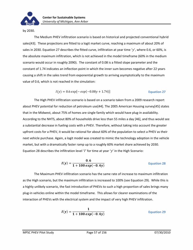
Center for Sustainable Systems University of Michigan, Ann Arbor
MPSC PHEV Pilot Study Page 57 of 156 07/30/2010
by 2030.
The Medium PHEV infiltration scenario is based on historical and projected conventional hybrid
sales[43]. These projections are fitted to a logit market curve, reaching a maximum of about 20% of
sales in 2030. Equation 27 describes the fitted curve, infiltration at year time ‘ ’, where 0.6, or 60%, is
the absolute maximum infiltration, which is not achieved in the model timeframe (60% in the medium
scenario would occur in roughly 2090). The constant of 0.08 is a fitted slope parameter and the
constant of 1.74 indicates an inflection point in which the inner sum becomes negative after 22 years
causing a shift in the sales trend from exponential growth to arriving asymptotically to the maximum
value of 0.6, which is not reached in the simulation:
0.6 0.08 1.74 Equation 27
The High PHEV infiltration scenario is based on a scenario taken from a 2009 research report
about PHEV potential for reduction of petroleum use[44]. The 2005 American Housing survey[45] states
that in the Midwest, about 75% of homes are single family which would have plug‐in availability.
According to the NHTS, about 80% of households drive less than 55 miles a day [46], and thus would see
a substantial decrease in fueling costs with a PHEV. Therefore, without taking into account the greater
upfront costs for a PHEV, it would be rational for about 60% of the population to select a PHEV as their
next vehicle purchase. Again, a logit model was created to mimic the technology adoption in the vehicle
market, but with a dramatically faster ramp up to a roughly 60% market share achieved by 2030.
Equation 28 describes the infiltration level ‘ ’ for time at year ‘ ’ in the High Scenario:
.
. Equation 28
The Maximum PHEV infiltration scenario has the same rate of increase to maximum infiltration
as the High scenario, but the maximum infiltration is increased to 100% (see Equation 29). While this is
a highly unlikely scenario, the fast introduction of PHEVs to such a high proportion of sales brings many
plug‐in vehicles online within the model timeframe. This allows for clearer examinations of the
interaction of PHEVs with the electrical system and the impact of very high PHEV infiltration.
. Equation 29

Center for Sustainable Systems University of Michigan, Ann Arbor
MPSC PHEV Pilot Study Page 58 of 156 07/30/2010
4.3 Electricity Generating Capacity Scenarios
Each year of the simulation, MEFEM checks to see if new electricity generating assets are required to
satisfy RPS or reserve margin requirements as outlined in subsection 3.3. This change in the mix of
assets in the system can affect the generators used to meet load due to PHEV demand. The size and
type of the assets created to meet these requirements are dictated by the electricity generating capacity
scenario being explored. Four scenarios are examined that influence the fuel mix of new generating
capacity by altering the RPS and the mix of generating capacity used to meet the reserve margin.
A Renewable Portfolio Standard (RPS) is state legislation that mandates a specified portion of
electricity generation to be met from renewable sources. In MEFEM, there are two possible RPS cases,
one based on an extended Michigan RPS and one that is based on the California RPS. In the Michigan
based RPS, the current legislation is used up to 2015, with targets for renewable generation being 2% by
2012, 5% by 2014, and 10% by 2015 [47]. In addition, the RPS is expanded in the model to include the
proposed 20% of generation by 2025 due to the push for renewable energy jobs in the state [28]. An
even more aggressive RPS scenario is loosely based off of the proportions and timing of the California
standard, with 20% by 2016, 29% by 2025 and 33% by 2026. For years without a concrete target, the
standards are interpolated between the two nearest goals. The percent of annual energy generation
that is required to be from renewable sources is shown in Figure 35 for both scenarios.
Figure 35. Renewable portfolio standard scenarios
New generating assets must be added to the grid to meet growth in peak electricity demand.

Center for Sustainable Systems University of Michigan, Ann Arbor
MPSC PHEV Pilot Study Page 59 of 156 07/30/2010
The methodology discussed in section 3.3 outlines how much new capacity is added each ear. The fuel
types of new plants are determined by the grid mix scenario. MEFEM has two possible grid mix
scenarios. One option is based on the national trends in new generating capacity creation as reported by
the EIA [20] and is labeled as the baseline grid mix scenario. The EIA only supplies data for the next few
years for new capacity, so everything after 2012 is assumed to have the same proportional new capacity
grid mix as 2012. The other grid mix option, named the high nuclear scenario, is identical to the baseline
grid mix except that all new coal generation is replaced with nuclear capacity after the year 2018. In
order to make a significant impact on the availability of nuclear generation, this scenario employs more
rapid retirements of the existing coal plants in Michigan, as discussed in Section 3.3. Figure 36 shows
the two scenarios’ capacity mix by fuel type as a function of the simulation year. These values are input
into the model to determine the proportional fuel mix of new generating capacity to meet peak
demand.
Figure 36. Grid mix scenarios
MEFEM has two possible RPS scenarios and two possible grid mix scenarios. Combinations of
these two option sets define the electricity generating capacity scenarios. Table 6 identifies the four
possible scenarios that are used in the model.
Table 6. Electricity generation capacity (EG) scenario inputs
Shorthand Title Scenario Number RPS Grid Mix
Baseline EG1 Michigan Baseline
High RPS EG2 Michigan High Nuclear
High Nuke EG3 California Baseline
High RPS/High Nuke EG4 California High Nuclear

Center for Sustainable Systems University of Michigan, Ann Arbor
MPSC PHEV Pilot Study Page 60 of 156 07/30/2010
4.4 Charging Scenarios
While the magnitude of the aggregated PHEV demand is determined by the selected PHEV infiltration
scenario, the shape of that demand is determined by the set of PECM inputs used to create the hourly
normalized PHEV load. Eight charging scenarios were developed to focus on the differences in time and
magnitude of PHEV charging demand due to changes in driver behavior, available charging
infrastructure and proposed utility imposed charging restrictions or price incentives. As outlined in the
methodology for PECM (subsection 3.1), the trip data is a set of actual trip schedules detailing when and
where a person travels. A charging scenario is comprised of a set of nine values, one for each of the nine
input parameters to PECM, each affecting the time, rate, and duration of the charging of an average
vehicle. Those parameters are charging location (CL), battery size (BS), charging current (CI) and voltage
(CV), charge onset delay (CD), minimum dwell time (MD), lower (NL) and upper (NU) bound of the no
charge window, and last minute charging.
The baseline charging scenario (CH1) represents the case in which a vehicle owner charges only
at home and begins charging as soon as they arrive. Charging occurs at the standard household wall
outlet rate of 12A, 120V. The battery size is loosely based on that of a Chevrolet Volt with a 65% eSOC
swing, yielding a usable battery size of 10.4 kWh. This scenario is considered the baseline because it
requires no adjustments, at home or at the utility, to infrastructure, and charging is only available to
drivers at home. Table 7 details the PECM model input parameters for every scenario.
Table 7. Charging (CH) scenario inputs to PECM
Scenario Name and Number
PECM Inputs
CL BS
(kWh) CI
(Amp) CV
(Volt) CD MD NL NU LM
Baseline CH1 Home 10.4 12 120 0 0 None None No
Last Minute CH2 Home 10.4 12 120 0 0 None None Yes
Home & Work CH3 Home & Work 10.4 12 120 0 0 None None No
Window CH4 Home 10.4 12 120 0 0 1pm 7pm No
Slow CH5 Home 10.4 8 120 0 0 None None No
Fast CH6 Home 10.4 16 240 0 0 None None No
Fast, H & W CH7 Home & Work 10.4 16 240 0 0 None None No
1/2 Battery CH8 Home 5.2 12 120 0 0 None None No
The last minute charging scenario (CH2) uses the same inputs as the baseline charging scenario,
but shifts the charging load to the last possible minute while ensuring a vehicle’s battery will reach its
maximum eSOC before the vehicle leaves on a trip. This requires that vehicle owners no a priori when

Center for Sustainable Systems University of Michigan, Ann Arbor
MPSC PHEV Pilot Study Page 61 of 156 07/30/2010
they will leave for a trip and that the vehicles have the capability to hold off charging until that moment.
Last minute charging has been identified as an effective way to reduce battery degradation for some
chemistries [19], and also may provide more of a demand leveling service to utilities (also generally
known as valley‐filling).
The home and work charging scenario (CH3) allows a vehicle owner to charge their vehicle at
work as well as home. The rate of charging and the battery size remain the same as the baseline, and no
extra constraints are added to the system. While it may not be widely available as yet, employers may
add charging stations to communal lots, increasing charging opportunities. With more charging
opportunities, a greater proportion of miles can be driven electrically, but with greater load on the
system.
The no‐charge window scenario (CH4) specifies a period, between 1pm and 7pm, in which
PHEVs are not allowed to charge their battery. This scenario is meant to represent a utility enforced
period in which vehicles are not allowed to charge to avoid times of peak electricity demand. This might
also lend some insight into situations where utilities use price incentives to force demand out of a peak
periods.
The slow charging scenario (CH5) adjusts the charging rate of the baseline scenario to 8A at
120V. This is meant to represent a charge rate that is compatible with older homes or a faulty
residential electric system and is one of the selectable charge settings on the Chevrolet Volt [17]. This
will should also reduce the peak of the charging load but make an average vehicle charge for more of
the day.
The fast charging scenario (CH6) increases the rate of charging from the baseline scenario to 16A
at 240V. This represents a homeowner who has installed a fast charging station at their residence and is
also one of the selectable charging rates of the Chevrolet Volt[17] . This scenario is expected to increase
the magnitude of peak charging but reduce its duration.
The seventh charging scenario combines fast charging with home and work charging. This
assumes that employers would have higher voltage charging available to their employees, and that
homeowners would also install these types of charge stations. This scenario represents the highest
amount of electricity consumption possible for the baseline battery size, using the parameter values
examined in this model.
The last charging scenario, CH8, halves the baseline usable battery size to gauge the effect that a
smaller battery has. This means that a given vehicle would have half the electric range, roughly 20 miles

Center for Sustainable Systems University of Michigan, Ann Arbor
MPSC PHEV Pilot Study Page 62 of 156 07/30/2010
for a compact car. However, this may not significantly alter the total percentage of electric miles driven,
since many of the trip schedules in the NHTS do not use the entire 10.4 kWh presented in the baseline
scenario. A half‐size battery would also make the purchase price of a PHEV more economical and would
lower the vehicle’s weight.
4.5 Electricity Dispatch Scenarios
The electricity dispatch scenarios examine the effect of the dispatch algorithm used and, if economic
dispatch is chosen, changes to a price‐based model of electricity generation. Three scenarios are
examined to test the models sensitivity to the dispatch algorithm employed. Table 8 describes the four
scenarios employed.
Table 8. Electricity dispatch scenario inputs
Scenario Name and Number Dispatch Method Fuel Price Source GHG Tax
Capacity Factor DM1 Capacity Factor ‐ No
BAU Economic DM2 Economic AEO 2010 No
GHG Tax DM3 Economic AEO 2010 Yes
The baseline scenario (DM1) uses capacity factor dispatch. As detailed in the dispatch
methodology section 3.4, capacity factor dispatch uses historical data to predict future behavior, with
the premise that those plants that were previously heavily utilized will continue to be used at roughly
the same rates. However, with new legislation pending to implement carbon taxes along with projected
changes in fuel prices, this assumption is not likely to remain accurate in the future. The economic
dispatch scenarios are designed to try and account for these future changes in generating costs.
The business as usual (BAU) economic dispatch scenario (DM2) sources the fuel costs from the
reference case of the AEO 2010 [39]. This scenario incorporates varying fuel costs, but does not include
any carbon legislation.
The GHG tax scenario (DM3) adds a cost in 2008$/ton CO2e to the emissions of greenhouse
gases to the fuel costs from the BAU economic dispatch case. Greenhouse gas emission rates are
determined using global warming potentials as described in subsection 3.5, and an emissions cost, based
on the EPA’s analysis of HR2454, is added to the fuel cost to get a total cost of generation. Figure 37
shows all the generation costs used by the scenarios.

Center for Sustainable Systems University of Michigan, Ann Arbor
MPSC PHEV Pilot Study Page 63 of 156 07/30/2010
Figure 37 Generation cost curves over simulation timeframe – all scenarios.
4.6 Simulations Analyzed
Table 9 below identifies the combinations of scenarios that are simulated and discussed in the results
section, Section 5. In addition, any simulation where marginal emissions of PHEVs are considered
requires an additional FI1 simulation to be run to see the interaction of the scenario parameters with
PHEV infiltration. For instance, calculation of marginal emissions in the FI4‐EG3‐CH1‐DM1 simulation
also requires there to be a FI1‐EG3‐CH1‐DM1 simulation, but these complimentary scenarios were not
explicitly listed in the table below for simplicity purposes. While Table 9 is not an exhaustive list of
potential simulations, these specific scenario combinations were selected to isolate scenario groups and
examine the effect of manipulating one parameter at a time.

Center for Sustainable Systems University of Michigan, Ann Arbor
MPSC PHEV Pilot Study Page 64 of 156 07/30/2010
Table 9. Full list of investigated simulations
Simulation Group
Name Fleet
Infiltration Electricity
Grid Charging
ElectricityDispatch
Fleet
Infiltration Baseline Zero FI1 EG1 CH1 DM1
Low FI2 EG1 CH1 DM1
Medium FI3 EG1 CH1 DM1
High FI4 EG1 CH1 DM1
Maximum FI5 EG1 CH1 DM1
Electric
Grid M
ix Baseline Generation Capacity FI4 EG1 CH1 DM1
High RPS FI4 EG2 CH1 DM1
High Nuclear Capacity FI4 EG3 CH1 DM1
High RPS/High Nuclear FI4 EG4 CH1 DM1
Charging
Baseline Charging FI4 EG1 CH1 DM1
Last‐minute Charging FI4 EG1 CH2 DM1
Home‐Work Charging FI4 EG1 CH3 DM1
No‐Charge Window FI4 EG1 CH4 DM1
Slow Charge FI4 EG1 CH5 DM1
Fast Charge FI4 EG1 CH6 DM1
Fast Charge at Home and Work FI4 EG1 CH7 DM1
Smaller Battery FI4 EG1 CH8 DM1
Electric Dispatch
Capacity Factor Dispatch FI4 EG1 CH1 DM1
BAU Economic FI4 EG1 CH1 DM2
GHG Tax FI4 EG1 CH1 DM3
Source list
Trip Data NHTS[46]
New vehicle sales MI MVR[22]
Vehicle sales growth AEO2009[20]
Low infiltration AEO2009[20]
Medium infiltration Lemoine 2008[43]
Historical HEV sales U.S. D.O.E, Alternative Fuels & Advanced
Vehicles Data Center, HEV Sales by Model[48]
High infiltration scenario Vyas2009[44]
Daily driving range to suit PHEV ownership Shiau Samaras 2009[49‐50]
Household statistics 2005 American housing survey[45]
Michigan RPS 2008 Clean renewable and efficient energy act[27]
High RPS CA RPS[51]
New capacity fuel mix proportions AEO2009[20]
Projected fuel costs AEO2009[20]

Center for Sustainable Systems University of Michigan, Ann Arbor
MPSC PHEV Pilot Study Page 65 of 156 07/30/2010
5. Results and Discussion
While the major results of the simulations are the total fuel cycle energy, greenhouse gas, criteria
pollutant emissions, and the gasoline displacement by PHEVs, to properly examine these results many
interim outputs of the model also must be presented. The PHEV Energy Consumption Model (PECM)
results are independent of the Michigan Electricity, Fleet and Emissions Model (MEFEM). PECM uses
nationwide travel survey data and its primary output is a weekly vehicle demand curve. For this reason,
PECM can be treated as a separate result and can be used for analyzing the response of PHEV infiltration
in any region. The following discussion in subsection 5.1 pertains solely to Michigan independent results
from the PECM simulations. The PECM results are input into MEFEM to assess the changes in
greenhouse gases (subsection 5.2), air criteria pollutants (subsection 5.3), total fuel cycle energy
(subsection 5.4), and gasoline displacement (subsection 5.5) for the Michigan system.
5.1 PHEV Energy Consumption Model Results
The outputs of PECM are primarily electricity usage and gasoline consumption for PHEVs. These results
will help to explain the emissions impacts of the charging scenarios examined later in Section 5.4. For a
more complete discussion of the PECM results see Appendix H.
While the outputs of PECM are size class specific, the following figures and results are based on
a light duty PHEV fleet with the size class distribution shown in Table 10. This distribution corresponds
to the PHEV distribution observed in the high fleet infiltration scenario, FI4, for the year 2030. Using a
weighted average result based on this distribution rather than all results for the individual size class
allows for a clearer presentation of PECM results.
Table 10. PHEV Fleet Distribution (based on 2030 High Fleet Infiltration Scenario)
Sub‐Compact Compact Midsize Large Van SUV Pickup
7.5% 19.5% 25.7% 10.6% 5.7% 21.8% 9.1%
5.1.1 Daily Variation in PHEV Consumption
In PECM, each day of the week is treated separately and the individual daily loads are strung together to
form weekly PHEV charging loads on the electric system. This subsection outlines some of the results of
this daily variation under baseline (CH1) charging conditions. Table 11 defines the inputs for the PECM
outputs discussed in this subsection.

Center for Sustainable Systems University of Michigan, Ann Arbor
MPSC PHEV Pilot Study Page 66 of 156 07/30/2010
Table 11. Input Parameters to PECM for Baseline Charging Scenario
Input Type [units] Code Baseline Value
Charging Location CL Home
Battery Size [kWh] BS 10.4
Charge Current [A] CI 12
Charge Voltage [V] CV 120
Charge Delay [min] CD 0
Minimum Dwell [min] MD 0
No‐Charge Lower Bound [hour] NL 0
No‐Charge Upper Bound [hour] NU 0
Last Minute Charging Flag LM 0
A seven day charging load for an average vehicle is shown below in Figure 38. The one week
time period represented along the horizontal axis begins on Tuesday at midnight. The vertical axis spans
a charging rate of 0 kW to 1.44 kW, which is the maximum charge rate of a single vehicle in the baseline
scenario (CH1). The highest peak in charging occurs at 8PM on most days. Wednesday evening shows
the highest charge rate, 0.707kW, which is 49% of the maximum possible charge rate, or 49% of vehicles
in the NHTS were charging at that time. Saturday evening, at 9PM, has the lowest peak, 0.503kW, which
represents 35% of the maximum charge rate. In this model charging load never drops to zero because
there are always vehicles charging at any time. The shape of the weekend loads differ from the
weekday loads with a wider bell shape and a more gradual peak. The anomalous peak between Sunday
night and Monday morning, circled in Figure 38, is due to the fact that disparate days are strung
together. The model uses Monday data to create the midnight hour between Sunday and Monday, thus
the magnitude of charging is higher because it actually represents the charging carried over from
Monday night loads. This discontinuity exists for each transition between days of the week, but is only
noticeable between Sunday and Monday.

Center for Sustainable Systems University of Michigan, Ann Arbor
MPSC PHEV Pilot Study Page 67 of 156 07/30/2010
Figure 38. Weekly charging load for the baseline scenario under a 2030 high fleet scenario distribution
Figure 39 displays the percent of electrically driven miles for each day in a one week time
period. The results display a fluctuation by day of the week in the percentage of driving propelled by
electric power ranging from 53.4% on Sunday to 63.6% on Tuesday.
Figure 39. Variation of the percentage of miles driven electrically by day of the week
5.1.2 Charging Scenario Analysis
The main output of PECM, used by MEFEM to evaluate impacts on emissions, is an hourly load curve
with PHEV electricity demand in kW per vehicle for every hour of the year. PECM generates seven sets
of normalized load curves, one for each vehicle size class, similar to the graph in Figure 38. These
charging load profiles are heavily influenced by the inputs to PECM. Table 4, in Section 4.4, indicates the
inputs into each of the eight charging scenarios. In order to understand their impacts on emissions, we
must first understand the impacts of the different charging scenarios on vehicle energy use. The graphs
Tue-12AM Wed-12AM Thu-12AM Fri-12AM Sat-12AM Sun-12AM Mon-12AM Tue-12AM0
0.2
0.4
0.6
0.8
1
1.2
1.4
Time of the Week
Norm
alized
Charging Load [kW
/veh]
Tuesday Wednesday Thursday Friday Saturday Sunday Monday0
20
40
60
80
100
Percent of Miles Drive Electrically [%]
Electric
Gasol ine

Center for Sustainable Systems University of Michigan, Ann Arbor
MPSC PHEV Pilot Study Page 68 of 156 07/30/2010
in Figure 40 display the average electricity and gasoline consumption per vehicle for each charging
scenario. Comparison of the two figures reinforces the intuitive inverse relationship between electricity
consumed and gasoline consumed, showing that as more electricity is consumed, less gasoline is
combusted. Energy consumption for all scenarios fluctuates around 50 kWh of electricity and roughly
four gallons of gasoline per week.
Figure 40. Energy consumption by charging scenario
The values of PHEV electricity consumption shown in Figure 40 are listed below in Table 12. The
electricity consumption rates for each scenario are also listed as a percentage change from the baseline.
The last minute charging scenario (CH2) shows no change in vehicle kWh consumption rates over
baseline charging (CH1) conditions, as last minute charging only shifts the time of charging and does not
affect the amount of charging that occurs. The scenarios that reduce electricity consumption are:
enforcing a no‐charge window (CH4), slow charging (CH5) and decreasing battery size (CH8). The smaller
battery size causes the greatest decrease in electricity consumption per vehicle and has the largest
impact on charging of any single parameter manipulation. On the other hand, the charging scenarios
responsible for an increase over baseline levels are: home and work charging (CH3), fast charging (CH6)
and the combination of the two, a fast charge home and work case, responsible for the sharpest rise in
vehicle energy consumption. The results show that the most important single parameter that effects
CH1 CH2 CH3 CH4 CH5 CH6 CH7 CH80
20
40
60
80Weekly Electricity Consumption for All Scenarios
Charging Scenario
Electricity Delivered
[kW
h/veh]
CH1 CH2 CH3 CH4 CH5 CH6 CH7 CH80
2
4
6Weekly Gasoline Consumption for All Scenarios
Charging Scenario
Gasoline Consumed
[gallons/veh]
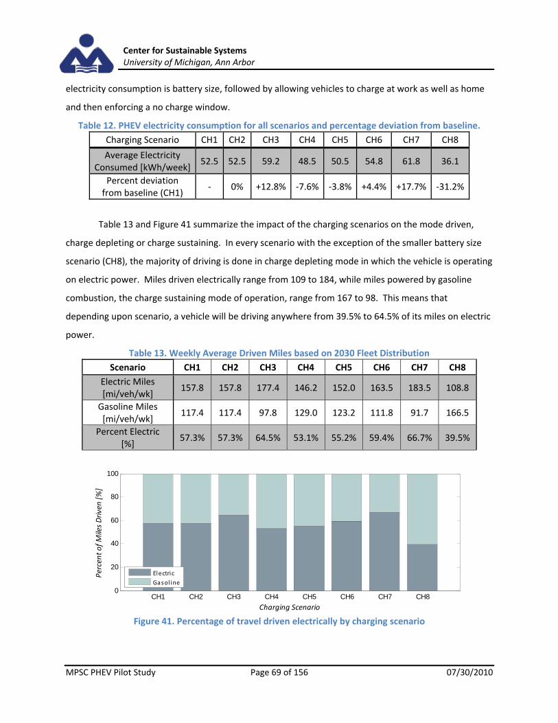
Center for Sustainable Systems University of Michigan, Ann Arbor
MPSC PHEV Pilot Study Page 69 of 156 07/30/2010
electricity consumption is battery size, followed by allowing vehicles to charge at work as well as home
and then enforcing a no charge window.
Table 12. PHEV electricity consumption for all scenarios and percentage deviation from baseline.
Charging Scenario CH1 CH2 CH3 CH4 CH5 CH6 CH7 CH8
Average Electricity Consumed [kWh/week]
52.5 52.5 59.2 48.5 50.5 54.8 61.8 36.1
Percent deviation from baseline (CH1)
‐ 0% +12.8% ‐7.6% ‐3.8% +4.4% +17.7% ‐31.2%
Table 13 and Figure 41 summarize the impact of the charging scenarios on the mode driven,
charge depleting or charge sustaining. In every scenario with the exception of the smaller battery size
scenario (CH8), the majority of driving is done in charge depleting mode in which the vehicle is operating
on electric power. Miles driven electrically range from 109 to 184, while miles powered by gasoline
combustion, the charge sustaining mode of operation, range from 167 to 98. This means that
depending upon scenario, a vehicle will be driving anywhere from 39.5% to 64.5% of its miles on electric
power.
Table 13. Weekly Average Driven Miles based on 2030 Fleet Distribution
Scenario CH1 CH2 CH3 CH4 CH5 CH6 CH7 CH8
Electric Miles [mi/veh/wk]
157.8 157.8 177.4 146.2 152.0 163.5 183.5 108.8
Gasoline Miles [mi/veh/wk]
117.4 117.4 97.8 129.0 123.2 111.8 91.7 166.5
Percent Electric [%]
57.3% 57.3% 64.5% 53.1% 55.2% 59.4% 66.7% 39.5%
Figure 41. Percentage of travel driven electrically by charging scenario
CH1 CH2 CH3 CH4 CH5 CH6 CH7 CH80
20
40
60
80
100p y y
Charging Scenario
Percent of Miles Driven [%]
Electric
Gasol ine

Center for Sustainable Systems University of Michigan, Ann Arbor
MPSC PHEV Pilot Study Page 70 of 156 07/30/2010
While the total amount of energy consumption is important, it is expected that the time at
which charging occurs may have a large impact on the emissions produced due to the type of generation
dispatched to meet that demand. Figure 42 displays the changes to the electric load profile (over a 24‐
hour period) with the addition of PHEV load for each PHEV charging scenario. The results shown in
Figure 42 are from the high infiltration simulation for the year 2030. In all eight subplots, the darker
shaded region represents the non‐PHEV base electrical load in Michigan in 2030 on a Tuesday in July,
chosen to represent a typical summer, high demand load. The lighter shaded region is the PHEV load in
2030 added to the non‐PHEV load. The light colored line plotted on top of the darker shaded region
represents the PHEV charging load profile independent of the base electric load. The load displayed
represents approximately 3,224,000 PHEVs on the road with the size class distribution described in
Table 10.

Center for Sustainable Systems University of Michigan, Ann Arbor
MPSC PHEV Pilot Study Page 71 of 156 07/30/2010
Figure 42. Aggregate PHEV load added to non‐PHEV load for a Tuesday in July 2030

Center for Sustainable Systems University of Michigan, Ann Arbor
MPSC PHEV Pilot Study Page 72 of 156 07/30/2010
In the baseline charging scenario (CH1), the majority of charging takes place after the
summertime peak occurs in the intermediate load level range. This has the effect of slightly increasing
the peak load while forcing the system to near peak capacity for an extended duration of the day. Last
minute charging (CH2) shifts most of the load into the times of least demand and in the morning hours
with only a slight increase in peak load. It has the effect of leveling out the load curve, which would
allow for more baseload capacity into the electric system. Home and work charging (CH3) increases
total energy consumption but distributes the PHEV load across the summertime peak demand. It
increases the peak slightly more than the baseline scenario and creates an extended peak period around
the existing one. Enforcing a no‐charge window (CH4) shifts a significant portion of the charging load
into off‐peak hours, but creates a new spike in load at 7PM that is larger than the original peak seen
under baseline charging conditions. This effect is due to PHEVs essentially queuing up to charge as soon
as they are allowed, and may be an undesirable effect of the this type of policy. The slow charging
scenario (CH5) flattens and spreads the charging load out over more of the day, avoiding much addition
to the peak but again extending the duration of peak loading. Fast charging (CH6) creates a large new
peak around 7PM. With PHEVs able to charge quickly, most of the load is occurring in the early evening
hours when many people come home from work, contributing to this new peak. Fast charging at home
and work (CH7) appears to reduce the size of the new peak observed in CH6 and distributes the charging
load over the summertime peak period. Almost no load is being added to the times of minimum
demand in this scenario. This implies that a fast charge scenario that employs last minute charging (not
examined here) may be the most efficient charging behavior at reducing the fluctuation in grid load. In
the smaller battery size scenario (CH8) there is a decrease in the magnitude of the charging load over
the baseline profile with most charging occurring in the evening hours.
The relative impact of PHEV charging loads on the electric system demand curve depends on
two factors: the number of PHEVS plugging‐in to the grid and the charging behavior. The graphs in
Figure 42 provide insight into the impact of PHEVs on the overall system load curve. Those of concern to
electric utilities are reductions in demand peaks, increases in off‐peak usage and shifts in demand from
peak to off‐peak times. The results of the charging scenarios demonstrate that, on a weekly basis, the
baseline charging (CH1), home and work charging (CH3), fast charging (CH6) and home and work fast
charging (CH7) cases require a large fraction of PHEV charging to occur during times of high peak or
moderate to high peak loads. The last minute (CH2) and slow charging scenarios show a more evenly
spread distribution of additional PHEV demand over the weekly load curve. Enforcing a no‐charge

Center for Sustainable Systems University of Michigan, Ann Arbor
MPSC PHEV Pilot Study Page 73 of 156 07/30/2010
window (CH4), from 1pm to 7pm, increases the minimum load but also creates a sharp new peak at 7pm
when the black‐out period ends.
5.1.3 Minimum Dwell time and Charge Onset Delay
The scenarios used in the MEFEM emissions analysis do not examine two of the possible inputs to PECM,
minimum dwell time and charge onset delay. This was done because the impact of the inputs on the
energy consumption and percent of miles driven electrically was too minimal to merit inclusion. PECM
was run with minimum dwell times of 30, 60, 90 and 120 minutes. In every case, the difference in
electricity consumed compared to baseline was less than 2% and there was almost no visible difference
in the shape of the charging curve. This slight change was not enough to expect to see any significant
changes in emissions results.
PECM was also run with 30 and 60 minute charge onset delays. This had a less than 1%
difference in the total amount of electricity consumed compared to the baseline scenario and simply
shifted the charging curve over by about one hour. This slight shift should not have a significant impact
on emissions results and, thus, was not included in the present analysis. A much larger charge onset
delay, causing a larger shift in the load curve, may have a significant emissions impact. However, since
the charge onset delay is meant to represent a period in which the vehicle hardware cools down, a much
larger delay seemed unreasonable.
5.2 Greenhouse Gas Emissions
The results from the PECM model described in 5.1 are used as inputs to MEFEM. To assess the impact of
PHEVs on greenhouse gas emissions, three greenhouse gases are tracked: Carbon Dioxide (CO2),
Methane (CH4), and Nitrous Oxide (N2O). All the results are presented in CO2 equivalents using global
warming potentials as defined by IPCC Fourth Assessment Report over the 100 year time horizon[38].
The specific scenarios analyzed to quantify greenhouse gas emissions are listed in tables at the
beginning of each of the following subsections.

Center for Sustainable Systems University of Michigan, Ann Arbor
MPSC PHEV Pilot Study Page 74 of 156 07/30/2010
5.2.1 Fleet Infiltration Implications
Table 14. List of simulations discussed for PHEV Fleet Infiltration
Simulations Fleet
Infiltration Electric Generation
Capacity Charging
Electricity Dispatch
Zero infiltration FI1 EG1 CH1 DM1
Low infiltration FI2 EG1 CH1 DM1
Medium infiltration FI3 EG1 CH1 DM1
High infiltration FI4 EG1 CH1 DM1
Max infiltration FI5 EG1 CH1 DM1
The number of PHEVs on the road has a significant influence on total fleet emission results. The
degree of this effect was investigated by running the simulations listed in Table 14, varying the
infiltration scenarios while holding the baseline charging (CH1), baseline electricity generating capacity
(EG1), and capacity factor dispatch methodology (DM1) scenarios constant.
The sales infiltration scenarios defined in Section 4.2 determine the number of PHEVs in the
light duty vehicle fleet. Figure 43 displays the number of PHEVs in the light duty vehicle fleet with
respect to simulation year for all sales infiltration scenarios. The inset plot shows the number of PHEVs,
in single units not millions, for the years 2014 through 2016. If approximately 3.3% of the U.S.
population resides in Michigan [52], one million PHEVs in the United States would translate to roughly
thirty thousand PHEVs in the state of Michigan. Under this assumption, the results of the medium
infiltration scenario align with the Obama administration’s goal for one million PHEVs on the road by
2015[1]. This same scenario has 13.3% of light duty vehicles as PHEVs in the final simulation year, 2030.
In the low infiltration scenario, PHEVs comprise 3.2% of the fleet in 2030. For the high and maximum
scenarios these percentages are 42.6 and 73.3, respectively.

Center for Sustainable Systems University of Michigan, Ann Arbor
MPSC PHEV Pilot Study Page 75 of 156 07/30/2010
Figure 43. Number of PHEVs on the road, 2010 ‐ 2030
Table 15 below shows the additional electricity (MWh) demand from PHEV addition to the grid
in the year 2030 for each infiltration scenario. These values are for PHEV infiltration under the baseline
charging (CH1) and baseline electric grid (EG1) scenarios.
Table 15. Additional electricity demand from PHEV infiltration, 2030 (CH1, EG1)
FI2 FI3 FI4 FI5
Total PHEV additional Demand (MWh)
719,566 3,000,861 9,596,797 16,531,227
Percent change from FI1 electricity demand (%)
0.60 % 2.49 % 7.96 % 13.71 %
In a fleet of purely conventional vehicles, transportation emissions are the sum of gasoline
combustion and upstream emissions. The addition of PHEVs to the fleet reduces total fuel cycle gasoline
emissions by displacing conventional vehicle gasoline use, but results in an increase in combustion and
upstream emissions from electricity generation. It is important to re‐emphasize the issue of emissions
allocation mentioned in previous sections. Note that total electricity emissions will be the same for a
given pathway regardless of the allocation method; However, the portion of emissions that should be
allotted to each demand source (i.e. lighting, HVAC, or, for the purposes of this study, PHEV batteries) is
under question. The simplest results to present, as they bypass this issue of allocation, are system wide
emissions which are defined as all transportation related emissions and all electricity related emissions
2010 2012 2014 2016 2018 2020 2022 2024 2026 2028 20300
2
4
6
8Millions of PHEV
2014 2015 2016
50,000
100,000
33,000*
Low PHEV infiltration (FI2)
Med PHEV infiltration (FI3)
High PHEV infiltration (FI4)
Max PHEV infiltration (FI5)
Total on‐road vehicles
73.3% PHEV
42.6% PHEV
13.3% PHEV
3.2% PHEV
No. ofPHEVson theroad

Center for Sustainable Systems University of Michigan, Ann Arbor
MPSC PHEV Pilot Study Page 76 of 156 07/30/2010
combined. Figure 44 and Table 16 provide system wide GHG emissions in the year 2030 for all fleet
infiltration scenarios.
Figure 44. Total GHG emissions for the year 2030 for all infiltration scenarios (EG1, CH1)
Table 16. Change in 2030 GHG Emissions due to PHEV addition (base grid scenario)
Change in EmissionsPHEV Scenario
Low Medium High Max
Total Electricity (billion kgCO2e)
0.35 1.44 4.48 6.29
Total Gasoline (billion kgCO2e)
‐0.75 ‐3.14 ‐10.02 ‐17.26
Net Change (billion kgCO2e)
‐0.40 ‐1.70 ‐5.54 ‐10.97
Deviation from ZeroPHEV Scenario (%)
‐0.4% ‐1.7% ‐5.4% ‐10.7%
Table 16 and Figure 44 illustrate the simultaneous increase in electricity emissions and decrease
in gasoline emissions for the year 2030. The resultant total emissions are lower in all infiltration
scenarios, with the difference from the zero PHEV simulation increasing with increasing infiltration.
Table 17 shows the size of the total emissions reduction created for the entire timeframe explored, in
which the summed emission totals for every year are compared. Here, the percent reduction in
emissions is much smaller due to the relatively slow PHEV infiltration for the first several years.
Zero Low Med High Max0
2
4
6
8
10
12x 10
10
Infiltration Scenario
kg GHG, Electricity and Transportation sectors
Total GHG emissions in 2030 for fleet scenarios, (Base grid/charging)
Electricity Upstream
Electricity Generation
PHEV Gasoline Upstream
PHEV Gasoline Combustion
CV Gasoline Upstream
CV Gasoline Combustion

Center for Sustainable Systems University of Michigan, Ann Arbor
MPSC PHEV Pilot Study Page 77 of 156 07/30/2010
Table 17. Change in full timeframe GHG Emissions due to PHEV addition.
Zero Low Med. High Max
Total Emissions 2009‐2030(billion kgCO2e)
2619 2616 2609 2588 2561
Total difference from Zero(billion kgCO2e)
‐ ‐3.19 ‐10.22 ‐31.06 ‐58.00
Deviation from Zero PHEV Scenario (%)
‐ ‐0.12% ‐0.39% ‐1.19% ‐2.24%
The next step is to allocate a portion of the emissions generated by electricity to the
transportation sector, and examine only transportation related emissions using the methodology
outlined in Section 3.5. Ascribing the net reduction seen in Table 16 to PHEVs is an example of marginal
emissions allocation.
In the marginal allocation method, emissions are assigned to PHEVs by comparing the emissions
from the PHEV scenario to the emissions in the base, zero PHEV scenario. In the PHEV scenario,
additional demand is placed on the system due to PHEV charging. To meet this demand, existing plants
are either utilized more, or new plants are built. The size of the new plants needed to meet RPS and
spinning reserve requirements is dependent on the number of PHEVs and the outputs of PECM. In
addition to the additional renewable generation due to the increase in electricity demand, more new
capacity will be added for reserve margin to accommodate PHEV load distributed over the annual peak
demand. New plants are given the characteristics of those found in Appendix B, which are cleaner and
more efficient than the initial assets in 2010. As per the stacking methodology, these plants will be
utilized before many of the older plants, and typically have lower emissions than older plants, as seen in
Appendix G. The majority of the difference in emissions due to the additional PHEV load will typically
come from these new plants. If the PHEV load is added to off‐peak demand, or ‘valley‐filling’, then while
the excess electricity requires more renewable energy to meet RPS, no new capacity will be necessary
for spinning reserve, and the demand for PHEVs will be met by existing, dirtier plants. This implies that
the marginal emissions of PHEVs will be lower if PHEV load is added to peak periods rather than off‐
peak.
Average emissions allocation analyzes the plants used to satisfy load at every hour, and
develops an average emission per kW for each hour. These hourly average emissions factors are then
applied to the PHEV load. The hourly average takes into account the entire generation mix. Adding new,
cleaner capacity reduces the average emission factor, but, unlike the marginal allocation methodology,
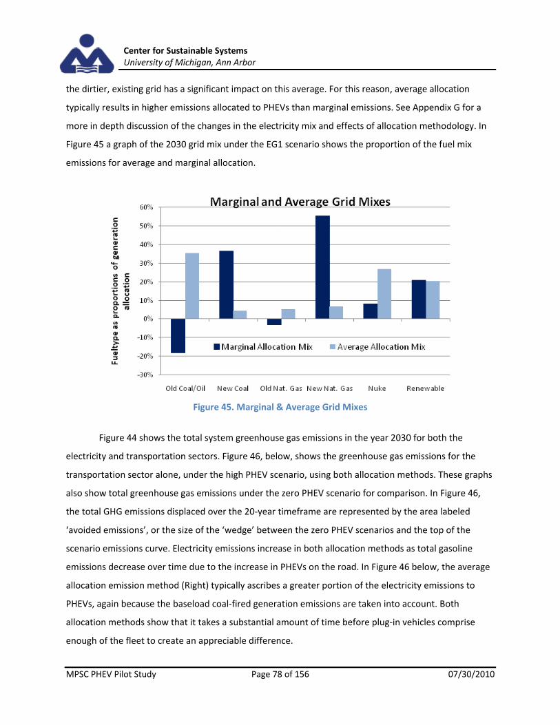
Center for Sustainable Systems University of Michigan, Ann Arbor
MPSC PHEV Pilot Study Page 78 of 156 07/30/2010
the dirtier, existing grid has a significant impact on this average. For this reason, average allocation
typically results in higher emissions allocated to PHEVs than marginal emissions. See Appendix G for a
more in depth discussion of the changes in the electricity mix and effects of allocation methodology. In
Figure 45 a graph of the 2030 grid mix under the EG1 scenario shows the proportion of the fuel mix
emissions for average and marginal allocation.
Figure 45. Marginal & Average Grid Mixes
Figure 44 shows the total system greenhouse gas emissions in the year 2030 for both the
electricity and transportation sectors. Figure 46, below, shows the greenhouse gas emissions for the
transportation sector alone, under the high PHEV scenario, using both allocation methods. These graphs
also show total greenhouse gas emissions under the zero PHEV scenario for comparison. In Figure 46,
the total GHG emissions displaced over the 20‐year timeframe are represented by the area labeled
‘avoided emissions’, or the size of the ‘wedge’ between the zero PHEV scenarios and the top of the
scenario emissions curve. Electricity emissions increase in both allocation methods as total gasoline
emissions decrease over time due to the increase in PHEVs on the road. In Figure 46 below, the average
allocation emission method (Right) typically ascribes a greater portion of the electricity emissions to
PHEVs, again because the baseload coal‐fired generation emissions are taken into account. Both
allocation methods show that it takes a substantial amount of time before plug‐in vehicles comprise
enough of the fleet to create an appreciable difference.

Center for Sustainable Systems University of Michigan, Ann Arbor
MPSC PHEV Pilot Study Page 79 of 156 07/30/2010
Figure 46. Transportation sector marginal and average emissions under high PHEV infiltration.
Figure 47 and Table 18 below, show the same trend of decreasing transportation sector
emissions due to the increase of plug‐in vehicles in the fleet, as well as the difference in emissions
between the allocation methods.
Table 18. Total fuel cycle GHG emissions (billion kg), transportation sector, 2030 (data for Figure 40)
FI Scenario Total Transportation Emissions (billion kg) Percent Change
Average Allocation Marginal Allocation Average Allocation Marginal Allocation
FI1 (Zero) 1,074 1,074 0.00% 0.00%
FI2 (Low) 1,071 1,070 ‐0.29% ‐0.30%
FI3 (Med) 1,064 1,063 ‐0.92% ‐0.95%
FI4 (High) 1,044 1,043 ‐2.72% ‐2.89%
FI5 (Max) 1,023 1,016 ‐4.73% ‐5.40%
These results are produced under baseline charging (CH1) conditions where the additional PHEV
demand increases the system peak load (reference Figure 37 in subsection 5.1.1). The model builds new
generation capacity to meet the additional demand when PHEVs are charged in the evening. These new
plants will have a higher capacity factor than some of the older plants of the same type and thus will be
used more often.
2010 2015 2020 2025 20300
2
4
6x 10
10
Year
kgGHGs produced
Transportation GHGs ‐ Marginal
Avoided Emissions
2010 2015 2020 2025 20300
2
4
6x 10
10
Year
kgGHGs produced
Transportation GHGs ‐ Average
Avoided Emissions
CV Gasoline Combustion
CV Gasoline Upstream
PHEV Gasoline Combustion
PHEV Gasoline Upstream
PHEV Electricity Combustion
PHEV Electricity Upstream
Base Case Transportation Emissions
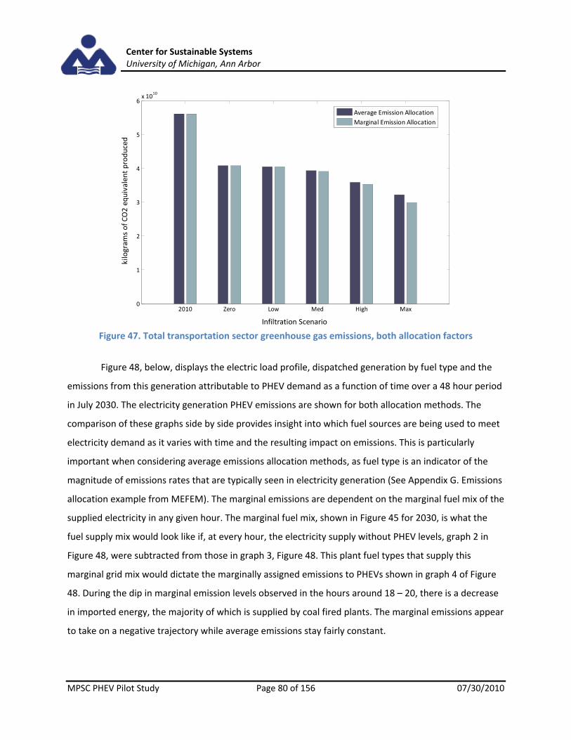
Center for Sustainable Systems University of Michigan, Ann Arbor
MPSC PHEV Pilot Study Page 80 of 156 07/30/2010
Figure 47. Total transportation sector greenhouse gas emissions, both allocation factors
Figure 48, below, displays the electric load profile, dispatched generation by fuel type and the
emissions from this generation attributable to PHEV demand as a function of time over a 48 hour period
in July 2030. The electricity generation PHEV emissions are shown for both allocation methods. The
comparison of these graphs side by side provides insight into which fuel sources are being used to meet
electricity demand as it varies with time and the resulting impact on emissions. This is particularly
important when considering average emissions allocation methods, as fuel type is an indicator of the
magnitude of emissions rates that are typically seen in electricity generation (See Appendix G. Emissions
allocation example from MEFEM). The marginal emissions are dependent on the marginal fuel mix of the
supplied electricity in any given hour. The marginal fuel mix, shown in Figure 45 for 2030, is what the
fuel supply mix would look like if, at every hour, the electricity supply without PHEV levels, graph 2 in
Figure 48, were subtracted from those in graph 3, Figure 48. This plant fuel types that supply this
marginal grid mix would dictate the marginally assigned emissions to PHEVs shown in graph 4 of Figure
48. During the dip in marginal emission levels observed in the hours around 18 – 20, there is a decrease
in imported energy, the majority of which is supplied by coal fired plants. The marginal emissions appear
to take on a negative trajectory while average emissions stay fairly constant.
2010 Zero Low Med High Max0
1
2
3
4
5
6x 10
10
Infiltration Scenario
kilogram
s of CO2 equivalent produced
Total Transportation Sector Greenhouse Gas Emissions ‐ 2030
Average Emission Allocation
Marginal Emission Allocation

Center for Sustainable Systems University of Michigan, Ann Arbor
MPSC PHEV Pilot Study Page 81 of 156 07/30/2010
Figure 48. Load, fuel mix and emissions, 2 days in July 2030 (base grid and charging, high PHEV)
5.2.2 Electricity Generation Capacity Implications
Table 19. List of scenarios discussed in Section 5.2.2.
Scenarios Electric Generation
Capacity Fleet
InfiltrationCharging
Electricity Dispatch
Baseline (MI RPS) EG1 FI1 & FI4 CH1 DM1
High RPS EG2 FI1 & FI4 CH1 DM1
High Nuclear EG3 FI1 & FI4 CH1 DM1
High RPS/High Nuclear EG4 FI1 & FI4 CH1 DM1
The previous subsections discuss how both the timing and total amount of PHEV energy demand
affect the emissions. Another important factor is the effect of changes in the generating capacity fuel
Center for Sustainable Systems University of Michigan, Ann Arbor
MPSC PHEV Pilot Study Page 82 of 156 07/30/2010
mix on these pathways and in turn how the new vehicle related grid demands impact power generation
requirements. Note that in the scenario table, Table 19, FI1 scenarios are listed to account for new
baseline scenarios. The results are the impact of PHEVs on a grid type, not the impact of different grid
types. The increase in electricity consumption from PHEV battery recharging under every grid scenario
for the high PHEV inciltration is 9,596,797 MWh.
The electricity generation capacity scenarios heavily influence the generation fuel mix of the
future grid. In Figure 49, below, the larger pie chart on the left displays the fuel mix of the Michigan grid
in the year 2009, the first year of simulation. The four pie charts on the right represent the fuel mixes for
the year 2030 under each of the four electricity generation capacity scenarios discussed in Section 4.3.
The results show that the implementation of a more aggressive RPS, like the one in the EG2 scenario,
results in fewer additions of coal and natural gas generating units, than the more modest RPS case of
EG1. This happens because building renewable plants to meet renewable requirements takes priority.
Under the EG3 (nuclear) and EG4 (high renewable and nuclear) scenarios, there is growth in natural gas
generation but a significant decrease in coal generation. This is caused by the generating unit retirement
schedule employed in these two scenarios. In EG3 and EG4, accelerated decommissioning of units
retires a substantial amount of coal capacity to allow for the addition of nuclear power. Only coal plants
are retired at an accelerated place in this retirement schedule, all other scheduled decommissioning
remain the same as EG1 and EG2.
All four scenarios result in a decrease of fossil fuel use in power generation over time, at varying
degrees compared to the 2009 fuel mix. This decrease is due mostly to the RPS scenarios employed, as
even the base case scenario assumes that the Michigan legislature will extend the current RPS from 10%
by 2015 to 20% by 2025, which is a substantially cleaner generation mix than the present.

Center for Sustainable Systems University of Michigan, Ann Arbor
MPSC PHEV Pilot Study Page 83 of 156 07/30/2010
Figure 49. 2030 Fuel mix for the four grid scenarios
Table 20 below, shows the full fuel cycle emissions (thousand tons) from electricity generation
in 2030 under each electric grid scenario. The fourth column in Table 20, difference in total system GHG
emissions, shows the percent increase in total fuel cycle GHG emissions from total system electricity
generation over the entire year of 2030 between the zero and high PHEV infiltration scenarios. The
aggressive renewable scenario, EG2, shows the greatest percent increase in total system emissions from
the addition of PHEVs to the grid. In the no PHEV case for this scenario a large amount of new
renewable generation capacity is built to satisfy the RPS requirements. These renewable additions
provide enough system capacity to meet the marginal capacity reserve requirement resulting in zero
non‐renewable plant additions. Since all new capacity has zero emissions, the total system capacity is
kept low. In the high infiltration case of the EG2 scenario, the additional PHEV load causes new plant
additions for the marginal capacity reserve requirement. In this case, the new capacity needs are met
with roughly 665 MW of natural gas and 440 MW of coal capacity. These changes are responsible for the
high percent change in system GHG emissions between the infiltration cases of the high renewable
scenario.
56%
9%< 1%
28%
4%3%Electricity Generation Fuel Mix in 2009
Coal
Natural Gas
Oil
Nuclear
Renewables
Imported
38%
12% < 1%
26%
20%
3%Base
17%
20%
< 1%39%
20%
3%High Nuclear
31%
7%< 1%
25%
33%
3%CA RPS
15%
16%
< 1%
33%
32%
3%High Nuclear & CA RPS

Center for Sustainable Systems University of Michigan, Ann Arbor
MPSC PHEV Pilot Study Page 84 of 156 07/30/2010
Table 20. GHG (kgCO2e) emissions comparison, 2030
EG Scenario Total System GHG emissions (FI1) ( thous. ton)
Total System GHG emissions (FI4) ( thous. ton)
Total System Difference (FI4 – FI1)
(%)
EG1 61,971 66,454 7.23%
EG2 49,255 53,098 7.80%
EG3 41,824 43,607 4.26%
EG4 35,690 37,161 4.12%
As the grid mix becomes successively cleaner, from electricity generation capacity scenarios EG1
through EG4, PHEV greenhouse gas emissions per mile (kgCO2e/mile) driven in the year 2030 are
reduced, as seen in Figure 50. Figure 50 along with Table 21 also displays the difference in emission
allocations methods, with greater reductions in marginal emissions than in average emissions. The error
bars indicate PHEVs driven in charge sustaining and charge depleting modes using both the nominal
marginal and average factors. The positive errors are the GHG emissions attributed to purely gasoline
consumption where as the negative error bars are those as if solely electricity was consumed to propel
PHEVs.
The difference in kilograms per mile between the average and marginal allocation methods is
small in EG2 compared to the other three electric grid scenarios. In EG2, the high RPS requirements
result in a large quantity of zero emission renewable capacity added to the system, the majority of
which is wind (90%). The addition of wind affects both marginal and average allocation because it is
applied to the system as a negative load. In the EG3 and EG4 scenarios, there are greater numbers of
generating asset retirements, necessitating the addition of more capacity to meet the MISO regulation.
The new capacity additions to meet reserve requirements do not include any renewable sources except
for a very small percentage (5 %) of LFG/biomass. The observed improvements in the CV fleet from 2010
to 2030, which are not present in the PHEV fleet, are due to the fact that fuel economy improvement
factors are applied to CVs. Therefore the kilograms per mile emission factors of PHEVs do not change
over the 20 year period like the CV fleet.

Center for Sustainable Systems University of Michigan, Ann Arbor
MPSC PHEV Pilot Study Page 85 of 156 07/30/2010
Table 21. Total fuel cycle GHG emissions per mile, 2030 (data for Figure 42)
kg / mile GHG (kgCO2e) / mile
CV, 2010 0.5298 EG
ScenarioAverage Marginal Difference
CV, 2030 0.3754 EG1 0.267 0.258 0.008
EG2 0.246 0.246 0.000
EG3 0.231 0.200 0.031
EG4 0.221 0.193 0.028
Figure 50. Per mile GHG emissions, 2030
The impact of each grid mix scenario on power generation greenhouse gas emissions are
provided in Table 22 below. The middle column represents the net change in emissions over the 20‐year
time period under all four scenarios for both the zero PHEV and high PHEV infiltration cases. The column
on the right displays the difference between the fleet infiltration cases under each grid mix scenario.
This column is the change in emissions from electricity generation attributable to PHEV energy
consumption; namely the impact of these new marginal demands on the grid.
CV only, 2010 CV only, 2030 Base Grid High RPS High Nuclear High RPS/Nuclear0
0.1
0.2
0.3
0.4
0.5
0.6
Ve
hic
ula
r G
HG
em
issi
on
s (k
gC
O2
e/m
ile)
Average Emission AllocationMarginal Emission Allocation
Upper Limit - Gas miles onlyLower Limit - Elec. miles only

Center for Sustainable Systems University of Michigan, Ann Arbor
MPSC PHEV Pilot Study Page 86 of 156 07/30/2010
Table 22. Percent change in electric sector GHG emissions, 2010 to 2030
Scenarios Change in GHG
emissions Impact of PHEV
additional demand
Base(EG1), FI1 ‐ 24.86% + 4.86%
Base(EG1), FI4 ‐ 20.00%
High RPS(EG2), FI1 ‐ 40.94% + 4.24%
High RPS(EG2), FI4 ‐ 36.70%
High Nuclear(EG3), FI1 ‐ 53.01% + 1.41%
High Nuclear(EG3), FI4 ‐ 51.60%
High RPS/High Nuclear(EG4), FI1 ‐ 60.39% + 1.04%
High RPS/High Nuclear(EG4), FI4 ‐ 59.35%
In the base case, greenhouse gas emissions from electric power generation decrease by
approximately 25% over the projection period, due to the imposed RPS standards. Adding PHEVs to the
grid increases electricity use, increasing electricity sector emissions, decreasing the net reduction from
the baseline scenario by 5%. The results of the other scenarios demonstrate how cleaning up the grid’s
predominately coal‐fired baseload assets produce a considerable decrease in associated greenhouse gas
emissions, of up to 60% in this study’s optimal scenario. Overall, these results indicate that policy‐
imposed constraints can command significant decreases in electricity generated greenhouse gas
emissions by forcing electric sector transitions to low CO2 generation. Furthermore, it supports the
replacement of dated and dirty coal plants with cleaner generation technologies to promote significant
emission improvements (per MWh generated), regardless of the size of PHEV charging load. If older
plants are taken off sooner and cleaner baseload generation is brought online, total emissions for the
grid will be greatly reduced over time, reducing the emissions allocated to PHEV. A higher RPS does
improve the grid, but increasing PHEV loads require the additions of “dispatchable” generation sources.
Dispatchable refers to those plants that are added to meet capacity marginal reserve requirements, or in
other words plants with high availability factors.

Center for Sustainable Systems University of Michigan, Ann Arbor
MPSC PHEV Pilot Study Page 87 of 156 07/30/2010
5.2.3 PHEV Charging Behavior Implications
Table 23. List of scenarios discussed in Section 5.2.3.
Scenarios Charging Fleet
InfiltrationElectric Generation
Capacity Electricity Dispatch
Base CH1 FI4 EG1 DM1
Last Minute CH2 FI4 EG1 DM1
Home & Work CH3 FI4 EG1 DM1
Blackout Window CH4 FI4 EG1 DM1
Slow Charge CH5 FI4 EG1 DM1
Fast Charge CH6 FI4 EG1 DM1
Fast Home & Work CH7 FI4 EG1 DM1
Smaller Battery CH8 FI4 EG1 DM1
As noted previously in Subsection 5.1, the charging habits of drivers affect the demand on the grid. As
this load changes, the assets which are dispatched to serve this demand will also change. Restrictions on
charging can also influence the amount electricity versus gasoline consumed by a PHEV driver. Figure 51
depicts the greenhouse gas emissions, in kgCO2e/mile, under different charging scenarios, for a high
PHEV infiltration, baseline electricity generation capacity, and capacity factor dispatch condition. Note
the differences amongst all eight charge cases between marginal and average allocation methods,
especially for the fast charge scenarios (CH6 and CH7). The pronounced differences for the fast charging
scenarios are due to high spikes in peak demand, as discussed in Section 5.1.2, which require a larger
amount of new capacity to be added to the system. Again, much of the affect to emissions from the grid
are tied to the amount of new capacity that is necessary. ‘Valley filling’ scenarios, such as last minute
charging or blackout periods do not increase the peak load, and therefore new capacity to meet
spinning reserve is not needed. Since these new, cleaner energy sources are not brought online, the
emissions associated are higher. Fast charging scenarios, CH6 and CH7, create a sharp spike in demand
near peak hours, and require the highest amount of new capacity. Since the new installed capacity
includes technology improvements, and as such is cleaner in than the existing generation, these
scenarios result in the lowest emissions.
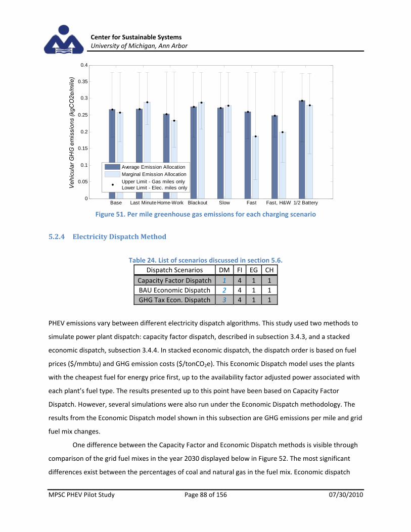
Center for Sustainable Systems University of Michigan, Ann Arbor
MPSC PHEV Pilot Study Page 88 of 156 07/30/2010
Figure 51. Per mile greenhouse gas emissions for each charging scenario
5.2.4 Electricity Dispatch Method
Table 24. List of scenarios discussed in section 5.6.
Dispatch Scenarios DM FI EG CH
Capacity Factor Dispatch 1 4 1 1
BAU Economic Dispatch 2 4 1 1
GHG Tax Econ. Dispatch 3 4 1 1
PHEV emissions vary between different electricity dispatch algorithms. This study used two methods to
simulate power plant dispatch: capacity factor dispatch, described in subsection 3.4.3, and a stacked
economic dispatch, subsection 3.4.4. In stacked economic dispatch, the dispatch order is based on fuel
prices ($/mmbtu) and GHG emission costs ($/tonCO2e). This Economic Dispatch model uses the plants
with the cheapest fuel for energy price first, up to the availability factor adjusted power associated with
each plant’s fuel type. The results presented up to this point have been based on Capacity Factor
Dispatch. However, several simulations were also run under the Economic Dispatch methodology. The
results from the Economic Dispatch model shown in this subsection are GHG emissions per mile and grid
fuel mix changes.
One difference between the Capacity Factor and Economic Dispatch methods is visible through
comparison of the grid fuel mixes in the year 2030 displayed below in Figure 52. The most significant
differences exist between the percentages of coal and natural gas in the fuel mix. Economic dispatch
Base Last Minute Home-Work Blackout Slow Fast Fast, H&W 1/2 Battery0
0.05
0.1
0.15
0.2
0.25
0.3
0.35
0.4V
ehi
cula
r G
HG
em
issi
ons
(kgC
O2
e/m
ile)
Average Emission Allocation
Marginal Emission Allocation
Upper Limit - Gas miles onlyLower Limit - Elec. miles only

Center for Sustainable Systems University of Michigan, Ann Arbor
MPSC PHEV Pilot Study Page 89 of 156 07/30/2010
utilizes much more coal than natural gas due to the high costs of natural gas compared to those of coal.
The economic dispatch method assigns power bands up to maximum proportion of the time the plant
would be available based on availability factor. Capacity factor dispatch assigns power bands based on
plant capacity factor, and caps maximum generation based on to the proportion of the actual unit’s
generation to the maximum theoretical energy the plant could provide on an annual basis.
Figure 52. Electric Fuel mix for 2030 for all three dispatch scenarios
The Michigan grid has a large amount of coal with an initial nameplate capacity of coal assets of
approximately 9,900 MW. If these coal assets were dispatched to their availability factors, the
generation would be roughly 50% greater than the actual output these plants produced according to
their historical capacity factors. Michigan is home to the second‐oldest fleet of baseload coal plants in
the nation with an average age of 49 years ([53]). The costs associated with dispatching older plants are
greater than those of newer plants. As plants age they require more maintenance. Over time, these
units will experience losses in thermal efficiency thereby requiring more fuel input per unit of energy
generated. The Economic Dispatch model dispatches coal to its availability factor adjusted power
because coal is a relatively cheap fuel source, and heat rates, which determine how much fuel a plant
consumes, remain unchanged throughout the years, as do emissions factors. Aside from fuel and
emissions prices, operational costs are not considered in dispatch decisions, which, due to the age of the
Michigan’s coal fleet, are not trivial. Since availability factors within the model are based on fuel type
averages, the output of older plants may be overestimated.
In the baseline scenario for economic dispatch, the model only considers the cost of fuel when
deciding how to dispatch the generating assets. In addition to fuel prices, the economic dispatch model

Center for Sustainable Systems University of Michigan, Ann Arbor
MPSC PHEV Pilot Study Page 90 of 156 07/30/2010
is designed to respond to greenhouse gas emissions costs which were modeled after those in the
Environmental Protection Agency (EPA) analysis of the American Clean Energy and Security Act, H.R.
2454 – GHG emissions and economic costs. However, as the results in Figure 52 show, a GHG emissions
tax at the level proposed in H.R. 2454 is not high enough to reduce coal‐fired electricity generation
within the state.
Another limitation of the Economic Dispatch model is the absence of seasonal variation in
natural gas prices, which may be one reason for the lack of natural gas generation present in the results.
This deficiency in natural gas generation has significant effects on the emissions attributed to PHEVs
between the two allocation methods. Both dispatch methodologies are stacked power dispatches; the
difference is the order and size of the stacks. As such, operating limitations or competitive market
considerations, such as minimum load levels, minimum stable operating levels, minimum run times,
generation efficiency decline, ramping rates, operation and maintenance costs, plant construction costs,
T&D costs, etc. are not modeled. These modeling assumptions have the greatest effect on generation
and dispatch results under the economic dispatch method. The ability of a plant to ramp up and down
(increasing or reducing output to meet fluctuations in demand) in response to changes in electricity
demand can vary with the fuel used to generate the electricity. For example coal plants have long ramp
up times. Therefore, they are predominately used as baseload or intermediate plants. Alternatively,
natural gas generators have fairly short ramp up times and thus are used to meet peak demands. Based
on these dispatch characteristics, baseload and intermediate plants that operate on a continuous basis
are generally coal fired generators while peaking plants that operate in an intermittent dispatch mode
are typically natural gas turbines. In real market conditions, natural gas turbines are dispatched to meet
peak demands despite their high fuel costs per MWh generated.
Table 25 shows the GHG emissions per mile for the PHEV fleet as it varies with electricity
dispatch and emissions allocation methods. The PHEV emissions under the average allocation method
vary by only 1.3% between the Capacity Factor Dispatch and Economic Dispatch under carbon cost
constraints scenario suggesting that during times when PHEVs are charging the instantaneous fuel mix
of the electricity grid is similar in both dispatch methodologies. Note that these results are for the
baseline charging scenario (CH1) where PHEVs charging predominately takes place during early evening
hours. On the other hand, under the marginal emission allocation method more extreme variations
occur between Capacity Factor Dispatch and Economic Dispatch under carbon costs constraints with a
16% increase in the DM3 scenario over Capacity Factor Dispatch. This difference between allocation

Center for Sustainable Systems University of Michigan, Ann Arbor
MPSC PHEV Pilot Study Page 91 of 156 07/30/2010
methods is due to the absence of natural gas in marginal generation supply in the Economic Dispatch
method. In the Economic dispatch simulations, marginal electricity demand is met by coal plants the
consequence of which is the assignment of a larger amount of coal emissions to the PHEVs. Marginally
assigned PHEV emissions are lower than those under the average allocation method in the case of
Capacity Factor Dispatch, but are higher in the Economic Dispatch method due to the differences in
intermediate and peaking generation fuel mixes.
Table 25. Comparison of PHEV per mile CO2eq emissions
PHEV fleet emissions rate(g CO2e/mile)
Dispatch Method
DM1 DM2 DM3
Average Allocation 271.5 269.1 267.9
Marginal Allocation
258.3 305.6 299.7
Marginally assigned PHEV emissions are lower than those under the average allocation method
in the case of capacity factor dispatch, but are higher in the economic dispatch method due to the
differences in intermediate and peaking generation fuel mixes between the methods. Under the average
emissions allocation method PHEVs are being assigned an average GHG emissions rate based on the
carbon intensity of all electricity generation in each hour. This remains relatively constant under the two
dispatch methods due to a high proportion of the generation, largely both the baseload and renewable
generation, being from nearly the same sources for each method. Under the marginal allocation
method, PHEVs are assigned the incremental GHG emissions from power plants operating during
battery recharging which would not be operating if PHEVs were not present, termed here as the
‘marginal mix’. Because the cost of generation of natural gas is much higher than that of coal, the
economic dispatch uses almost exclusively coal power in its marginal mix. In the capacity factor
dispatch, the marginal mix is largely the existing natural gas peaking plants and new, cleaner generation.
This difference in fuel mix accounts for the high variation in marginal results between the two methods.
Other studies have used similar methods to the economic model employed in the present analysis, and
a similar tendency to allocate high emissions on the margin was observed in the results of the study by
Axsena, Kurania, McCarthy and Yang at University of California, Davis[54]. These high emissions in
marginal allocation suggest that simplified economic dispatch methods should not be used with
marginal allocation methods as they do not account for many of the complexities inherent to the

Center for Sustainable Systems University of Michigan, Ann Arbor
MPSC PHEV Pilot Study Page 92 of 156 07/30/2010
electricity dispatch. These complexities include generator ramping constraints (coal‐fired generation is
much slower to ramp up to full power than natural gas turbines), transmission congestion, and seasonal
variability in fuel prices. A capacity factor dispatch may be more suited to marginal allocation
methodologies because it is inferred that these complexities are inherent to capacity factor, a quantity
based on historical generation, despite its limited ability to adjust to changing market environments.
Since the Capacity Factor Dispatch method is based on historical power plant capacity factors, it
more accurately simulates the split between baseload power plants and peaking generators. In contrast,
the Economic Dispatch model uses the cheapest power supply source to meet electricity demands,
regardless of whether this generation is for base, intermediate or peaking load. Despite the many
shortcomings of this study’s Economic Dispatch model relative to its Capacity Factor Dispatch method, it
does have the ability to simulate a future market where carbon intensive electricity is less utilized, and
cleaner fuels such as natural gas constitute a greater portion of the generation mix. The GHG emissions
tax scenario, based on H.R. 2454, does not cause a significant turnover in generation mix. The capacity
decision model can already simulate a significant change in the fuel mix from input guidelines such as
accelerated retirement scheduling, aggressive RPS and high nuclear scenarios, but those changes are
through pre‐defined parameters, rather than on real time price‐based conditions. In theory, economic
dispatch represents the most accurate simulation of real world conditions. However, in order to mimic
the behavior of the competitive electricity market, the model would need to be able to perform asset
valuations on a spatially and temporally nodal basis. As the limitations of the current Economic Dispatch
model dictate the results, this report has focused on the Capacity Factor Dispatch model results.
5.3 Criteria Air Pollutant Emissions
Table 26. List of scenarios discussed in subsection 5.3
Simulations FI EG CH DM
Baseline electricity generation PHEV (5.3.1) 1 & 4 1 1 1
Cleanest electricity generation PHEV (5.3.2) 1 & 4 4 1 1
In the previous subsections, the environmental consequences of PHEV infiltration have only been
presented as changes in greenhouse gas emissions. Implications to Michigan air quality involve the
examination of other atmospheric emissions. Six common air pollutants, defined as criteria pollutants by
the EPA and regulated under the Clean Air Act [55], are as follows: Carbon Monoxide (CO), Lead (Pb),
Nitrogen Oxides (NOX), Particulate Matter (PM2.5 and PM10), Ozone (which is created at ground‐level via

Center for Sustainable Systems University of Michigan, Ann Arbor
MPSC PHEV Pilot Study Page 93 of 156 07/30/2010
chemical reaction between NOX and volatile organic compounds, VOCs), and Sulfur Dioxide (SOX). The
Michigan Electricity, Fleet and Emissions Model (MEFEM) calculates the emissions for CO, Pb, NOX,
PM2.5, PM10, VOC, and SOX. Note this study does not account for any potential new emission controls
required in future regulations.
5.3.1 Total system air pollutant emissions
In the following discussion, total system emissions in 2030 are compared for simulations with
and without PHEVs under the baseline electricity generation capacity scenario (EG1) and simulations
with and without PHEVs under the cleanest electricity generation scenario (EG4). The results are
presented as a percent change from the zero PHEV case (FI1). The results in Figure 53 are for EG1
conditions and those displayed in Figure 54 are for the EG4 case. These figures are shown to
demonstrate the net effect of PHEV infiltration on the entire Michigan system and how these effects
change depending on two potential cases for the Michigan 2030 generation capacity fuel mix. A
complete table of fuel specific, per mile emissions factors for electricity generation and gasoline usage
can be found in Appendix K.
Total system emissions results display increases in SOX for both electric grid cases and increases
in Pb and PM10 pollutant levels for the EG1 scenario. The increases seen are related to the shift towards
electrically driven miles, in which case the electric sector is a more prominent source of pollution than
gasoline on a per mile basis. Total system emissions include all electricity generation and transportation
sector emissions. Since oil plays such a small role in electricity generation in the initial year, and is not
considered an option for new capacity generation, oil electric generation effects are omitted from the
following discussion of criteria pollutant emissions. Between the FI1 and FI4 simulations for EG1 oil is
the only generation fuel that experiences a net decrease. A net decrease as used here would indicate
that more plants of this fuel type are retired or have their power bands decreased than are added as
new generation capacity to the system. A net increase would indicate the opposite effect. In the EG4
simulations, there is a net decrease in oil and coal.
In both figures there is an observed decrease in CO emissions when PHEVs are added to the
fleet because gasoline has significantly higher total fuel cycle CO emission rates than electricity
generation from any fuel type.
The increase in Pb emissions shown in Figure 53 is due to the fact that electricity demands for
PHEV recharging causes additional generation capacity. The data source used for gasoline use does not

Center for Sustainable Systems University of Michigan, Ann Arbor
MPSC PHEV Pilot Study Page 94 of 156 07/30/2010
track Pb emissions, despite the fact that it may be present in upstream processes, and therefore a
reduction in gasoline consumption cannot decrease Pb emissions. Under EG1 new capacity needs are
met mainly by new natural gas and coal generation both of which have Pb emissions. The decrease in Pb
emissions under EG4 shown in Figure 54 is caused by the replacement of coal generation with nuclear
generation between grid scenarios in addition to the accelerated retirements of coal assets in EG4.
NOX emission levels decrease in the base grid scenario because all electricity generation fuels
have lower NOX emission rates than gasoline. The total change in electricity generated NOX emissions
due to PHEV infiltration is a net decrease in coal power generated and a net increase in natural gas
electricity. Natural gas electricity has the lowest NOX emissions rate outside of nuclear generation and
renewables. The further decrease of NOX in EG4 is due to the reduction of coal generation because coal
has the highest NOX emission rates of all electricity fuel sources.
PM2.5 emissions are significantly decreased in both grid scenarios due to the fact that the data
set used for electricity generation does not specify a difference between particulate matter emissions,
and they were all classified as PM10 emissions. Therefore, the change in PM2.5 emissions is directly
related to gasoline displacement.
PM10 increases slightly in the base grid scenario because coal, the predominant energy source in
the grid mix, has a greater PM10 emission levels than gasoline, although other fuel types used in this
study for electricity generation are lower than both gasoline and coal. New power plants have the same
PM10 emission rates as existing assets of the same fuel type. In the clean grid case these emissions
decrease as nuclear replaces coal in the fuel mix. The emissions levels of PM10 are less because more
coal assets are retired in this scenario.
VOC levels decrease in both generation scenarios due to the displacement of gasoline by PHEV
infiltration. Gasoline has higher VOC emission rates than any electricity generation source, even though
within the model, new power plants are modeled with the same VOC emission rates as old plants of the
same fuel type. Although VOC levels increase due to increased electricity demand from PHEVs, the
majority of which is from increased natural gas generation, the corresponding decrease in VOC
emissions from gasoline displacement results in a net decrease in total system full fuel cycle emissions.
Total SOX emissions increase in both generation scenarios when PHEVs are added. New coal
plants, built to serve the additional load, have much lower SOX emissions rates than existing plants.
However, because the majority of SOX emissions for natural gas occur in the upstream phase, the
technology improvements applied to new plants do not have as large an effect on total natural gas

Center for Sustainable Systems University of Michigan, Ann Arbor
MPSC PHEV Pilot Study Page 95 of 156 07/30/2010
emissions rates. The technology characteristics for new and existing (averages) plants can be found in
Appendix K. While gasoline displacement, especially counting the avoided upstream gasoline emissions,
reduces the overall SOX emitted in the system, the prevalence of natural gas and coal generation within
the system results in a net increase in SOX emissions. It should also be noted that SOX emissions caps are
not taken into account in the model and therefore generation emissions from existing plants may be
inflated.
Figure 53. Change in total system emissions between FI1 and FI4 (EG1, CH1, 2030)
Figure 54. Change in total system emissions between FI1 and FI4 (EG4, CH1, 2030)
The well‐to‐wheel changes in system wide criteria air pollutant emissions with the addition of
CO Pb NOx PM2.5 PM10 VOC SOx‐25
‐20
‐15
‐10
‐5
0
5
10
Percen
t Change from FI1
CO Pb NOx PM2.5 PM10 VOC SOx‐25
‐20
‐15
‐10
‐5
0
5
10y g ( )
Percent Chan
ge from FI1

Center for Sustainable Systems University of Michigan, Ann Arbor
MPSC PHEV Pilot Study Page 96 of 156 07/30/2010
PHEVs to the fleet are summarized below in Table 27.
Table 27. Percent change in total system criteria air pollutants.
CO Pb NOX PM2.5 PM10 VOC SOX
Percent change EG1 ‐22% +4% ‐5% ‐25% +0.1% ‐15% +5%
Percent change EG4 ‐23% ‐2% ‐9% ‐25% ‐7% ‐17% +7%
5.3.2 Transportation sector air pollutant emissions
In this subsection, transportation sector emissions in 2030 are broken out from total system emissions
and examined by each emission allocation method. They are compared for simulations with high PHEV
infiltration between the baseline electricity generation capacity scenario (EG1) and the cleanest
electricity generation scenario (EG4) for both emission allocation methods. The results are presented as
a percent change from the zero PHEV case (FI1), with Figure 55 displaying emission levels under EG1
conditions and Figure 56 showing these same emissions under the EG4 case.
In both grid scenarios, CO, PM2.5 and VOC emission levels all decreased by roughly the same
magnitude between marginal and average allocation methods. The reason there is no discrepancy in
between allocation methods for these pollutants is because it is the displacement of gasoline that is
responsible for the majority of the change in emissions rather than electricity generation changes.
Although lead increased in the system due to added electricity demand, it is not displayed in the figures
because the base FI1 scenario has zero lead emissions and therefore a percent increase could not be
calculated.
NOX emissions increase in the case of average emissions because natural gas represents a larger
proportional piece of the fuel mix with PHEVs than without them, while coal and nuclear, both of which
have lower NOX emission rates than natural gas, represent a slightly smaller portion of the fuel mix in FI4
than they did in FI1. However, in the case of marginal allocation, NOX emissions decrease because
marginal emissions are more closely associated with new capacity additions in the system to meet the
added PHEV demand. This is because the addition of PHEV charging loads causes existing plants to be
used less while new plants meet the new load. The case of NOX new power plants have greatly improved
emissions rates over their existing counterparts. In EG4, the same reasoning stands for the decrease in
marginal NOX emissions. In the case of average emissions, NOX levels decrease because of overall grid

Center for Sustainable Systems University of Michigan, Ann Arbor
MPSC PHEV Pilot Study Page 97 of 156 07/30/2010
improvements.
PM10 emission levels increase with both allocation methods. There is a much larger increase in
average PM10 emissions because even though coal is reduced in the grid, new plants are modeled with
the same PM10 emission rates as old plants and coal electricity generation is a very heavy emitter of
PM10. IN EG4, PM10 levels decrease under both allocation methods. This is due to the accelerated coal
retirements under this scenario as well as the greater proportion of nuclear (a cleaner burning fuel in
terms of PM10) than coal in EG4.
In both grid scenarios SOX levels increase because electricity generation emits more SOX than
gasoline. In EG1, marginally allocated emissions are lower than those on the average because the added
generation to serve PHEV load are power plants with improvements in SOX emission rates. Marginal
emissions are closely associated with new capacity additions. In EG4, emissions are reduced compared
to EG1. However the marginally allocated emissions do not decrease as much because in EG4 there are
accelerated retirements of existing coal assets along with fewer new coal plants added to the system.
Coal powered generating units have the greatest technology improvements, vastly reducing the SOX
emission rates of new coal generation. In EG1 the addition of PHEVs requires the addition of new
generating assets, including new coal, making marginally allocated SOX levels lower than the average
grid, which is influenced by existing coal at 40% of total generation. However in EG4, existing coal is
removed in greater numbers than EG1 but not replaced with any new coal generation so while the
entire grid does in fact improve with respect to SOX as shown by the decrease in average emissions, the
marginally allocated emissions in EG4 do not receive the same “benefit” as in EG1 from the coal
technology improvements.
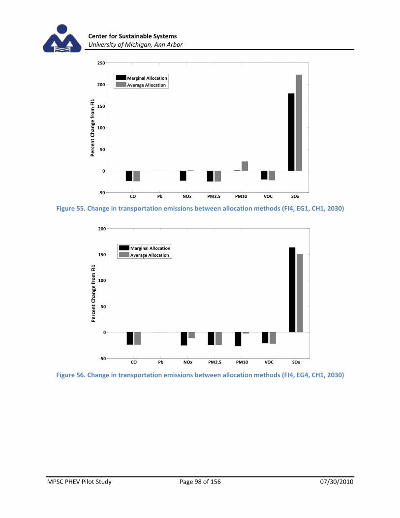
Center for Sustainable Systems University of Michigan, Ann Arbor
MPSC PHEV Pilot Study Page 98 of 156 07/30/2010
Figure 55. Change in transportation emissions between allocation methods (FI4, EG1, CH1, 2030)
Figure 56. Change in transportation emissions between allocation methods (FI4, EG4, CH1, 2030)
CO Pb NOx PM2.5 PM10 VOC SOx‐50
0
50
100
150
200
250
Percent Change from FI1
p g ( , , )
Marginal Allocation
Average Allocation
CO Pb NOx PM2.5 PM10 VOC SOx‐50
0
50
100
150
200
Percent Change from FI1
Marginal Allocation
Average Allocation
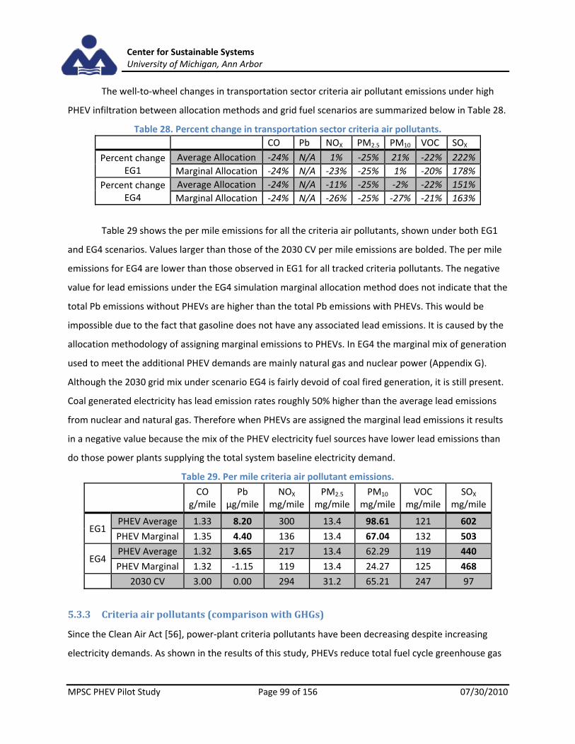
Center for Sustainable Systems University of Michigan, Ann Arbor
MPSC PHEV Pilot Study Page 99 of 156 07/30/2010
The well‐to‐wheel changes in transportation sector criteria air pollutant emissions under high
PHEV infiltration between allocation methods and grid fuel scenarios are summarized below in Table 28.
Table 28. Percent change in transportation sector criteria air pollutants.
CO Pb NOX PM2.5 PM10 VOC SOX
Percent change EG1
Average Allocation ‐24% N/A 1% ‐25% 21% ‐22% 222%
Marginal Allocation ‐24% N/A ‐23% ‐25% 1% ‐20% 178%
Percent change EG4
Average Allocation ‐24% N/A ‐11% ‐25% ‐2% ‐22% 151%
Marginal Allocation ‐24% N/A ‐26% ‐25% ‐27% ‐21% 163%
Table 29 shows the per mile emissions for all the criteria air pollutants, shown under both EG1
and EG4 scenarios. Values larger than those of the 2030 CV per mile emissions are bolded. The per mile
emissions for EG4 are lower than those observed in EG1 for all tracked criteria pollutants. The negative
value for lead emissions under the EG4 simulation marginal allocation method does not indicate that the
total Pb emissions without PHEVs are higher than the total Pb emissions with PHEVs. This would be
impossible due to the fact that gasoline does not have any associated lead emissions. It is caused by the
allocation methodology of assigning marginal emissions to PHEVs. In EG4 the marginal mix of generation
used to meet the additional PHEV demands are mainly natural gas and nuclear power (Appendix G).
Although the 2030 grid mix under scenario EG4 is fairly devoid of coal fired generation, it is still present.
Coal generated electricity has lead emission rates roughly 50% higher than the average lead emissions
from nuclear and natural gas. Therefore when PHEVs are assigned the marginal lead emissions it results
in a negative value because the mix of the PHEV electricity fuel sources have lower lead emissions than
do those power plants supplying the total system baseline electricity demand.
Table 29. Per mile criteria air pollutant emissions.
CO
g/mile Pb
μg/mileNOX
mg/milePM2.5
mg/milePM10
mg/mileVOC
mg/mile SOX
mg/mile
EG1 PHEV Average 1.33 8.20 300 13.4 98.61 121 602
PHEV Marginal 1.35 4.40 136 13.4 67.04 132 503
EG4 PHEV Average 1.32 3.65 217 13.4 62.29 119 440
PHEV Marginal 1.32 ‐1.15 119 13.4 24.27 125 468
2030 CV 3.00 0.00 294 31.2 65.21 247 97
5.3.3 Criteria air pollutants (comparison with GHGs)
Since the Clean Air Act [56], power‐plant criteria pollutants have been decreasing despite increasing
electricity demands. As shown in the results of this study, PHEVs reduce total fuel cycle greenhouse gas

Center for Sustainable Systems University of Michigan, Ann Arbor
MPSC PHEV Pilot Study Page 100 of 156 07/30/2010
emissions compared with CVs because most CO2 is emitted from the burning of gasoline. While GHG
emissions are global emissions, interpretation of criteria pollutant results is more complex as the
impacts of criteria pollutants are location and time dependent. Therefore, criteria air pollutant
emissions from mobile tailpipe cannot be considered equally to emissions from stationary power
sources. PHEVs produce emissions at both sources.
The results imply that a switch from a conventional vehicle to a PHEV operating in charge
depleting mode (all electrical miles) will reduce overall air pollution (except sulfur emissions), and this
net benefit is even more pronounced under a less carbon intensive grid. However, the model does not
categorize the emissions as point sources. The model looks at the total emission at only state‐level
resolution. The PHEV CD mode of operation displaces emissions from where more vehicles are driven to
where power plants are located. These effects are not accounted for, and as a result, some places will
experience a reduction in emissions while some will see air pollutants increasing, as seen in the PHEV
study by Thompson, Webber and Allen[12]. However, it may be simpler to regulate emissions from
hundreds of stationary power plants than from millions of vehicle tailpipes.
5.4 Total Fuel Cycle Energy
Figure 57 displays the per mile total fuel cycle energy for electric‐driven miles. The total fuel cycle
energy, or well‐to‐wheels energy, includes all life cycle energy used to drive the vehicle, from mining,
processing and transporting fuels to vehicle propulsion. The black dotted line represents the average
energy per mile need to propel the vehicle. This value, 0.30 kWh/mile (1.06 MJ/mile), is marked off to
serve as a reference point, the electrical energy needed solely for vehicle propulsion while in charge
depleting mode. In general, energy consumed above this line can be ascribed to electricity generation
and upstream energy. Again, note the discrepancy between emission allocation methods in the fast
charge scenarios, where the grid has experienced a greater number of clean capacity additions.

Center for Sustainable Systems University of Michigan, Ann Arbor
MPSC PHEV Pilot Study Page 101 of 156 07/30/2010
Figure 57. Per mile primary energy for each charging scenario.
All the charging simulations are based on the base future grid mix scenario. When comparing across
different generation mixes, the high nuclear scenarios had an increase in per mile energy for PHEVs,
while the High RPS scenario reduced the total fuel cycle energy, likely as facility production energy was
omitted and electricity supplied by wind, hydro, or LFG had zero associated total fuel cycle energy.
2030 CV Base Last Min. Home-Work Blackout Slow Fast Fast H&W 1/2 Batt.0
1
2
3
4
5
6V
eh
icu
lar
TF
C E
ne
rgy
con
sum
ed
(M
J/m
ile)
Average Energy Allocation
Marginal Energy Allocation
Upper Limit - Gas miles onlyLower Limit - Elec. miles only

Center for Sustainable Systems University of Michigan, Ann Arbor
MPSC PHEV Pilot Study Page 102 of 156 07/30/2010
Figure 58. Per mile primary energy for each grid mix scenario.
5.5 Gasoline Displacement
The volume of gasoline displaced by electrically driven miles is calculated for each scenario. The
amount of gasoline consumed on a per‐vehicle basis is a direct output of the PHEV Energy Consumption
Model (PECM). These values are applied to each infiltration scenario, with each PHEV displacing a
conventional vehicle in the same size class. This vehicle substitution results in a net reduction of
gasoline. The volume of gasoline displaced over each PHEV infiltration scenario, under the base charging
(CH1) and base grid mix, is shown in Table 30, along with the proportion of gasoline used in year 2030
compared to the year 2009. That is, due to improvements in the CV fleet alone, Michigan will only use
73% of the gasoline in 2030 as it did in 2009.Bringing many PHEVs online can reduce the state’s use to
less than half that.
Table 30. Gasoline displacement (millions of gallons) by PHEV fleet infiltration scenario, 2010 ‐ 2030
PHEV Fleet Infiltration Scenario
FI1 (Zero) FI2 (Low) FI3 (Med.) FI4 (High) FI5 (Max)
TFC Gasoline displacement From PHEV infiltration (M gal)
0 574 1,782 5,273 9,084
Percent of yearly use from 2009
73% 71% 67% 55% 42%
As Table 15 shows, PHEVs increase electricity use. Table 30 shows that increasing the number of
CV only, 2010 CV only, 2030 Base Grid High RPS High NuclearHigh RPS/Nuclear0
1
2
3
4
5
6
7
8
Ve
hic
ula
r T
FC
En
erg
y co
nsu
me
d (
MJ/
mile
)
Average Energy AllocationMarginal Energy Allocation
Upper Limit - Gas miles onlyLower Limit - Elec. miles only

Center for Sustainable Systems University of Michigan, Ann Arbor
MPSC PHEV Pilot Study Page 103 of 156 07/30/2010
on‐road PHEVs decreases the state’s gasoline needs. Table 31 displays the gallons of gasoline displaced
for each PHEV charging scenario under the high PHEV infiltration and base grid mix scenarios.
Table 31. Gasoline displacement (millions of gallons) by PHEV charging scenario, 2010 ‐ 2030
Charging Scenario
CH1 (Base)
CH2 (LM)
CH3 (H&W)
CH4 (Window)
CH5 (Slow)
CH6 (Fast)
CH7 (Fast H&W)
CH8 (1/2 Batt.)
Gasoline Displacement
(Mgal) 5,273 5,273 5,889 4,907 5,094 5,452 6,081 3,750
Deviation from baseline (%)
0% 0% +11.68% ‐6.94% ‐3.39% +3.39% +15.32% ‐28.89%
% ofyearly use from 2009
54.7% 54.7% 52.5% 56.0% 55.3% 54.1% 51.8% 60.0%
The displaced gasoline volumes shown in Table 31 are dependent on the results of the PECM
model, specifically the gasoline/electric miles split seen in Table 13 in subsection 5.1.2. For each PHEV, a
greater proportion of miles driven in electric mode translates to a larger displacement of gasoline. Each
charging scenario was conducted under a high PHEV infiltration rate; each simulation has the same
number of PHEVs. However, comparing Table 30 and Table 31, it can also be seen that while the timing
and amount of charging has an effect, increasing the number of vehicles on the road would have a larger
cumulative effect on reducing the state’s gasoline needs. Many PHEVs are better than few PHEVs, but
for a single PHEV, more gasoline is displaced in earlier years than in later years because of the CV
improvements seen in Table 30. These gasoline reduction figures do not account for the petroleum
used to generate electricity as energy from oil constitutes a negligible fraction of the total Michigan
electrical energy supply. The fuel mix of generated electricity does not contribute to any of the
reductions in gasoline consumption seen in these results.
5.6 Comparison to other studies
As mentioned in the literature review (subsection 2.1), many previous studies have examined
the per mile emissions of PHEVs. Figure 59 shows a collection of per mile greenhouse gas (GHG)
intensities for PHEVs (grams of CO2e per mile) in several of the studies discussed in subsection 2.1, with
varying color bars signifying the range of results reported in those studies. The darkest shaded portions
represent the values of GHG intensity found in studies that report only a singular emissions level or the
lowest value found in studies that present a range of per mile GHG results. The lightest shaded bars
symbolize the upper limit of GHG per mile intensities that pertain to studies which reported a range of

Center for Sustainable Systems University of Michigan, Ann Arbor
MPSC PHEV Pilot Study Page 104 of 156 07/30/2010
results. The results from MEFEM are displayed on the right most side of the graph for comparison.
The wide range of per mile emissions stems from the methodology used by the research groups.
For example, the two bars furthest to the left that represent studies by Keoleian and Sullivan, used the
same energy consumption factors for PHEVs but assumed different grid CO2 intensities to achieve
different results. EPRI, which has the lowest, studied PHEV emissions from a 2050 electricity generation
grid. Overall per mile emissions ranged from 125 to 477 gCO2e/mile.
The range of MEFEM results, from 193 to 280 gCO2e/mile, is based on the highest and the
lowest marginally assigned emissions from all scenario sets studied under high PHEV infiltration. The
highest emissions were found from the ½ battery simulation (FI4 EG1 CH8, Figure 51), which is expected
as the highest proportion of gasoline driven miles was in that scenario. The lowest emissions were seen
in the High RPS, High Nuclear Electricity Generation simulation (FI4 EG3 CH1, Figure 50), which had the
lowest GHG grid intensity. Scenarios such as fast charging in a High RPS, High Nuclear grid would
probably have lower emissions per mile from coupling the high electric‐to‐gasoline miles ratio with at
cleaner grid, but this simulation was not investigated in depth, and was not included in creating this grid.
Again, the differences in scope of the various studies makes it difficult to compare results.
However, the fact that the results of this study are within the range of previous, similar studies adds
credibility to the assumptions and methodology used.
Figure 59. GHG emissions results comparison with other studies
Center for Sustainable Systems University of Michigan, Ann Arbor
MPSC PHEV Pilot Study Page 105 of 156 07/30/2010
6. Conclusions and Recommendations
The objectives of this study were to determine and evaluate the environmental impacts of widespread
PHEV adoption in the state of Michigan from 2010 to 2030.
Two models were developed to examine the effect of emissions from potential future pathways
for PHEV battery charging, fleet infiltration, and changes to electricity generation that PHEV introduction
may create. The first model, the PHEV Energy Consumption Model, begins by determining the individual
PHEV electricity demand profiles and gasoline use under a range of vehicle charging assumptions and
actual trip patterns from a national daily travel database. In the Michigan Electricity, Fleet and Emissions
Model, these demand profiles are scaled by the number of PHEVs on the road as defined in the selected
infiltration scenario. The total electricity demand for PHEVs is added to the state’s baseline electric load
and modeled as a single node using average transmission line loss without any further considerations of
the system’s nodal constraints. New electricity generating capacity is added to the system to meet RPS
and spinning reserve requirements when necessary. Plants are dispatched to meet hourly demand
based on Michigan specific historical plant capacity factors or the cost of generation. The final results
are total fuel cycle energy consumed and emissions of greenhouse gases and criteria air pollutants.
These are reported as a system total or allocated to the transportation sector using both marginal and
average methodologies. Total transportation sector gasoline displacement is also reported.
While increasing PHEVs reduces gasoline consumption, the extent to which PHEVs can decrease
emissions will depend mainly on the impacts to the electric grid from an increasing number of these
vehicles in the fleet. A set of scenarios were constructed to explore key variables including market
infiltration rates, PHEV user charging and driving behavior, vehicle design characteristics such as battery
size and efficiency, and future mixes of electricity generating capacity technologies and their dispatch
order. Based on the analysis of simulation results, the team has developed a number of conclusions,
recommendations and suggestions for future work which are summarized below.
6.1 Key Findings
Increasing the number of PHEVs in the Michigan fleet reduced net greenhouse gas emissions at every
infiltration level (Subsection 5.2)
The shift from gasoline‐ to electricity‐fueled travel yielded a net reduction in total fuel cycle
greenhouse gas emissions in every explored simulation, despite the additional emissions from electricity

Center for Sustainable Systems University of Michigan, Ann Arbor
MPSC PHEV Pilot Study Page 106 of 156 07/30/2010
generation. This reduction in total statewide greenhouse gases from electricity and transportation,
under the baseline charging and electricity grid mix, ranged from 0.4 to 11.0 billion kgCO2e in 2030, a
0.4% to 10.7% reduction, depending on the infiltration level. Over the course of the 20 year timeframe,
infiltration of PHEVs reduced total GHG emissions by 3 to 58 billion kgCO2e, depending on the infiltration
level. The relationship between PHEV infiltration and GHG emissions reductions was not linear, with
higher infiltration levels having a disproportionately greater impact on GHG emissions reduction. Total
fuel cycle emissions of a PHEV, per mile driven, ranged from 275 to 240 gCO2e per mile in 2030
depending upon the allocation method and the infiltration scenario used. For reference, an average
conventional vehicle in 2010 emitted 530 gCO2e per mile and in 2030 it was expected to emit 375 gCO2e
per mile. PHEVs in 2010 emitted 268 gCO2e per mile in the model.
PHEV infiltration caused a decrease in the level of certain criteria air pollutants but an increase in
others (Subsection 5.3)
CO, NOX, and VOC total system emission levels were reduced as a result of PHEV infiltration
under both grid mix scenarios. However, total system SOX emissions increased at each level of PHEV
infiltration in all electricity generation scenarios. In the baseline electricity generating capacity case,
particulate matter emissions increased (PM10 up 0.1%) but the percent increase was very small
compared to that of SOX (increase of 5%). In the high nuclear and high RPS generating capacity case, only
SOX increased. The especially high SOX is largely due to the fuels consumed for electricity generation
versus gasoline, but the results may be inflated because the dispatch model used in this study did not
take sulfur caps into account nor advances in SOX ‘scrubbing’ into account.
However, while some emissions did increase, these are local emissions at a limited number of
power plants. An air quality model of the region is needed to understand the potential impacts of these
local emissions, but it should be noted that the benefit of emitting from a small number of sources,
compared to distributed emissions among a vehicle fleet, is that it may be much cheaper and easier to
mitigate said emissions.
When transportation sector emissions were isolated from total system emissions, the same
general trends were observed, but in the cases of particulate matter, SOX and NOX large discrepancies
existed between marginal and average allocation methods because emissions from new capacity and
older natural gas‐fired power plants were weighted more heavily toward PHEVs in the marginal
allocation method than the average allocation method. The average allocation method assigned a
Center for Sustainable Systems University of Michigan, Ann Arbor
MPSC PHEV Pilot Study Page 107 of 156 07/30/2010
higher percentage of coal generation, which had higher emissions rates than the new capacity and
natural gas plants (with SOX being the only exception), giving the average allocation method higher
emissions than the marginal.
PHEVs have lower total fuel cycle energy use than conventional vehicles (Subsection 5.4)
Total fuel cycle energy, or well‐to‐wheels energy use for PHEVs, under the baseline charging and
electric grid mix scenarios was lower than that of the average per mile rate of the CV fleet. In MEFEM,
conventional vehicles in 2030 had a fuel economy of 30 miles per gallon. These vehicles consumed 5.2
MJ per mile, accounting for both upstream and combustion energy. Depending on the allocation
method, the CH1 scenario on road PHEVs consumption ranged from 3.8 to 4.2 MJ per mile in the base
grid scenario. Since the per mile total fuel cycle consumption is lower for PHEVs, increasing the number
of PHEVs in the fleet reduces the total transportation sector energy use.
PHEVs can significantly reduce the state’s gasoline consumption (Subsection 5.5)
Gasoline displacement increased as the number of PHEVs increased in the simulation. High
infiltration reduces gasoline consumption by 25% in 2030 compared to a completely conventional
vehicle fleet. By the year 2030, between 574 and 9084 million gallons of gasoline were displaced when
compared to the scenario without PHEVs. Within the model, the consumption rates of conventional
vehicles improved annually, but the consumption rates of PHEVs did not. Because PHEV technology
does not improve, the benefits of a single PHEV are reduced over time. Therefore, the actual gasoline
displacement as infiltration increases may increase if PHEV technology improvements were included in
the model.
Total system greenhouse gas emissions were modestly affected by the shape and magnitude of the
PHEV charging load (Subsection 5.2.3)
The total fuel cycle system emissions were affected by charging assumptions in the high PHEV
scenario. In 2030, the charging scenarios examined in this report showed between a 3.3% reduction
(fast charging) and a 1.5% increase (last minute charging) in GHG emissions when compared to the
baseline charging scenario. These two fast charging scenarios showed the greatest reduction in most
emissions, largely due to the increase in the annual peak load. This increase resulted in a need for more
new generating capacity within the model to meet spinning reserve requirements. New capacity was

Center for Sustainable Systems University of Michigan, Ann Arbor
MPSC PHEV Pilot Study Page 108 of 156 07/30/2010
assumed to be cleaner than existing generators, having the characteristics displayed in Appendix B. The
last minute charging scenario posted the greatest increase in emissions because most of the load was
added in the hours of least demand, which was largely coal‐fired generation and reduces the amount of
new capacity needed to meet demand.
The shape of the normalized charging curve for a single PHEV is significantly affected by changes
to charging behavior. A fast charge can create a large spike in the aggregate behavior, a larger battery
will increase the magnitude and duration of charging, last minute charging will shift the load to the
times of least demand, and instituting periods in which a vehicle cannot charge creates an instantaneous
peak when the window ends.
While these differences in the shape of the charging curve are not significant until there are a
large number of PHEVs in the LDV fleet, for any number of PHEVs, greater proportions of miles driven in
electric mode tend to decrease GHG emissions.
Imposing a period of time in which vehicles cannot charge to avoid additional peak demand
seems to have less desirable results than intended. Enforcing this makes all PHEV consumers in the
model simply wait until the no‐charge window is lifted to plug in, creating a very significant peak in a
later hour. The no‐charge window scenario had among the highest per mile greenhouse gas emissions of
any charging scenario examined with a 1.4% increase over the baseline scenario. One way to mitigate
this peak may be to stagger the start time of PHEVs through demand side management controlled by
the utility’s smart grid.
Last minute charging was the most effective strategy to shift load into off peak hours. In order
to implement last minute charging, vehicles will have to come equipped with software that allows users
to set the time they expect to leave in the morning such that the vehicle can estimate the latest possible
time to begin charging. However, last minute charging increased emissions in most categories as less
new capacity is brought online and it allows more generation to be met by existing baseload coal‐fired
plants.
The greatest GHG emissions and energy use of any charging scenario occurred in the smaller
battery scenario, due to the decrease in electrically driven miles. An examination of continually
increasing battery size, found in Appendix H, revealed a strong coupling of battery size to the
percentage of electrically driven miles. However, it also showed that the rate of increase diminished as
battery size grew. This suggests an interesting trade‐off: while larger batteries allow for more
electrically driven miles, smaller batteries will be more economical and many consumers may opt for

Center for Sustainable Systems University of Michigan, Ann Arbor
MPSC PHEV Pilot Study Page 109 of 156 07/30/2010
smaller battery sizes if their commute does not require larger range. This suggests that an optimization
of battery size, GHG reductions, and cost may be an interesting direction for further research.
Renewable generation and accelerating the retirement of coal‐fired power plants improve
transportation sector greenhouse gas emissions (Subsection 5.2)
By simulating a high RPS, nearly 33% of Michigan’s electricity needs could be provided by clean,
renewable sources. However, because of the nature of our dispatch model, the large addition of
renewable sources had the effect of replacing natural gas generation. This is not a realistic result since
peaking plants will be required to even out these intermittent power sources. If the model correctly
accounted for ramping constraints, more natural gas utilization would be observed. As more natural gas
generation is added to the system to complement renewable intermittent generation, a larger decrease
in GHG emissions may be seen as less coal‐fired generation will be utilized.
Other simulations showed that retiring older coal plants to bring nuclear baseload generation
online resulted in much lower emissions both overall and due to PHEVs. In the base grid scenario, PHEVs
increased greenhouse gas emissions related to electricity by about 5%. The high RPS scenario decreased
this to 4.2%. The high nuclear simulation, which accelerates the retirement of coal‐fired baseload and
builds more nuclear generation, served the PHEV load with only a 1% increase in greenhouse gas
emissions, while reducing the overall grid GHG emissions to 40% of the original 2009 grid. In this high
nuclear scenario in 2030, coal generation is approximately 25% less than in the baseline grid mix
scenario, going from 50% of total generation to 37%, and nuclear generation increases from 26% to 39%
of total generation.
When examining the effects of a changing grid, removing older plants and increasing new, cleaner
generation decreases criteria air pollutant emissions compared to a baseline grid scenario, but SOX
emissions still increase with PHEV infiltration (Subsection 5.3)
Higher PHEV infiltrations increase the need for new generation, and by bringing cleaner sources
of generation online, emissions are reduced. However, the sulfur content of the fuels used to generate
electricity, especially the upstream SOX emissions of natural gas generation, is much higher than the
intensity of SOX in the avoided gasoline. Therefore, while cleaning the grid reduces the total emissions in
the electricity generation sector, more PHEVs increase SOX emissions in the transportation sector.
Center for Sustainable Systems University of Michigan, Ann Arbor
MPSC PHEV Pilot Study Page 110 of 156 07/30/2010
The addition of renewable generation can reduce total fuel cycle energy (Subsection 5.4)
Since renewable generation was modeled without any manufacturing energy, it has no
associated total fuel cycle energy. Thus, increasing the amount of renewable generation in the system
has a significant impact on the PHEV’s total fuel cycle energy. By retiring coal plants and increasing
nuclear and natural gas generation, the high nuclear scenario had a greater effect on emissions than the
high RPS scenario. However, PHEVs within the high RPS scenario had the lowest energy consumption per
mile travelled, at 3.5 MJ/mile, while the high nuclear scenario increased PHEV energy use per mile to
above the base scenario rates. For all the grid scenarios, PHEV energy use per mile was still lower than
CV energy use.
6.2 Recommendations
PHEV adoption should be encouraged within the state
In every scenario extrapolating a future Michigan grid, increasing the infiltration of PHEVs
decreased greenhouse gases, transportation energy, and most criteria pollutants. Increasing PHEVs also
reduced the state’s petroleum use.
To avoid creating new peaks in electricity demand, more charging locations and last minute charging
are the best strategies
Utilities may be interested in avoiding new peaks in electrical demand to minimize the need for
new peaking capacity in the future. The goal is then to both spread out the PHEV demand and to move it
to off peak hours, which is best simulated by the last minute charging and the home‐work scenario.
Fast charging would force new, cleaner generation into the grid; however, this would come about by
creating new peaks in the system electrical demand that, in this model, creates the need for new cleaner
generating capacity. Home and work charging provides a similar electric‐to‐gasoline miles ratio as fast
charging, and home and work charging produces similar reductions in GHG emissions to fast charging
without creating such large peaks in demand using the average allocation method. If the goal is to avoid
creating large peaks while still increasing total electric miles driven, then investments in work charge
infrastructure will work better than investments in fast charge infrastructure.
To bring about the greatest environmental improvements, Michigan’s aging coal‐fired power plant
fleet should be retired and replaced with cleaner generating sources

Center for Sustainable Systems University of Michigan, Ann Arbor
MPSC PHEV Pilot Study Page 111 of 156 07/30/2010
While adding renewable generation does improve the grid, simulations in which coal plants that
were retired at age 60 and replaced with cleaner sources showed significant decreases in greenhouse
gas emissions. When the grid was improved, the additional emissions attributed to PHEVs were also
reduced.
A standardized methodology for assigning electricity generation emissions due to PHEV charging is
needed
The method of assigning electricity generation emissions to PHEVs needs to be standardized.
The marginal allocation methodology only attributes the emission from generation units that are
brought online to meet the additional load to PHEVs which in this model are typically new plants in the
later years. However, under the average allocation method, the existing generation also comprises a
large component of emissions assigned to PHEV loads. To definitively quantify the environmental effects
of PHEVs, an allocation method must be chosen.
6.3 Future Work
The study identifies some of the complexities associated with analyzing an integrated system of
transportation and electric sectors. Depending on the power level, timing, and duration of the PHEV
connection to the grid, there could be a wide variety of impacts on grid constraints, capacity needs, fuel
consumed, and emissions generated. Some areas that could be more fully explored include:
Incorporating other alternative fueling strategies for light duty vehicles
Within this study, vehicles were modeled as either plug‐in electric hybrid or conventional
gasoline fueled vehicles. The emissions factors for gasoline include a small amount of blended ethanol,
but this ratio is fixed within the model. In the future, vehicles may use alternative fuels such as
biodiesel, petroleum diesel, natural gas, 85% ethanol or other biofuels. Further work could investigate
the effects on emissions and gasoline displacement from the incorporation of these fuels into the
model.
Adjusting PHEV Consumption parameters using trip data
In the PHEV Energy Consumption Model, PHEVs consume the same amount of gasoline and

Center for Sustainable Systems University of Michigan, Ann Arbor
MPSC PHEV Pilot Study Page 112 of 156 07/30/2010
electricity, regardless of the type of trip. A modeling approach that uses the average speed and distance
of a vehicle trip to determine a more probable average consumption rate for that trip may add greater
accuracy to the results of the simulations.
Developing PHEV technology improvements within PECM
PHEVs in the model have the fuel consumption characteristics listed in Appendix F which are based on
pre‐production and academic sources in 2009. While conventional vehicles have continually improving
fuel economies, PHEV characteristics do not change in the model. PHEVs are also expected to improve
over time, and modeling this would improve emissions results.
Using daily travel distance to inform PHEV trip profiles
In some cases, PHEVs will not be used as often for certain types of trips, or may not make sense for
those who have very short or long commutes. For instance, a driver whose daily commute is 10 miles
will not need a PHEV capable of driving 40 miles on a single charge, since a PHEV with smaller battery or
even a conventional hybrid may be more economical. On the other hand, for someone whose daily
driving patterns greatly exceed 40 miles, most of the driving will be comparable to a conventional
hybrid. If the trips that PECM uses to develop PHEV energy consumption results represent only those
likely of a PHEV driven in specified ways, more realistic charging strategies and charging profiles could
be created.
Exploring a greater range of charging scenarios
The selected set of charging simulations provided insight as to how time and magnitude of
charging affected the electric grid and subsequent emissions. Exploring more scenarios, such as different
or multiple daily no‐charge windows, or more combinations of the selected scenarios, will provide more
possible pathways and a clearer picture of how utility or design controls affects demand control and
emissions.
Staggering no‐charge windows to simulate the effect of demand side control
In its current form, enforcing a no charge window creates a large instantaneously ramped peak
at the end of the window. This may be mitigated by staggering windows to flatten out the load. In
addition, this may more accurately represent how customers may respond to price incentives as they

Center for Sustainable Systems University of Michigan, Ann Arbor
MPSC PHEV Pilot Study Page 113 of 156 07/30/2010
will likely not all wait for the window to end before they begin charging.
Employing blended charging strategies
All PHEVs will not be charging under the same conditions. It is likely that actual PHEVs in the
fleet will employ many of the different scenarios outlined and combinations of some of the parameters
in those scenarios. The scenarios provided represent the bounds of the actual energy consumption
patterns of PHEVs: i.e. it is unlikely that all PHEV owners will have access to fast charge infrastructure
(CH6). Development of a blended energy consumption representation that is a weighted average of the
different charging scenario results may provide a more accurate picture of what will be seen at large
fleet infiltration levels. In addition, these weighted averages could be used to determine optimal
scenarios for specific utility needs, such as filling in the valley in daily demand curves.
Developing the electricity generation and dispatch further
Capacity factor dispatch is employed with the underlying assumption that future dispatch will be
similar to the dispatch of the previous year. Outside factors that change the economics of electricity
generation, such as new taxes or regulations, would skew the dispatch order in real life but would not
be captured by the capacity factor dispatch methodology. Also, the proportion of imported power was
held constant and used only to serve peak demand, but this is not necessarily the case for the Michigan
grid.
Other power dispatch characteristics not captured in the current model include minimum run
times for facilities, minimum load levels, and physical constraints on ramping rates and associated
ramping emissions.
While a large fleet of PHEVs could theoretically be accommodated within Michigan at current
capacity levels, depending on when or where vehicles are plugged in load transmission and distribution
constraints could arise at local or regional levels. The model’s current treatment of demand and
generation as point sources is a great simplification. The current economic dispatch model also assumes
that fuel prices are constant all year, which is not accurate for natural gas. A further developed
economic dispatch would allow better research into the effects of emissions pricing, especially with a
more sophisticated transmission and distribution methodology and more time variability in fuel prices.
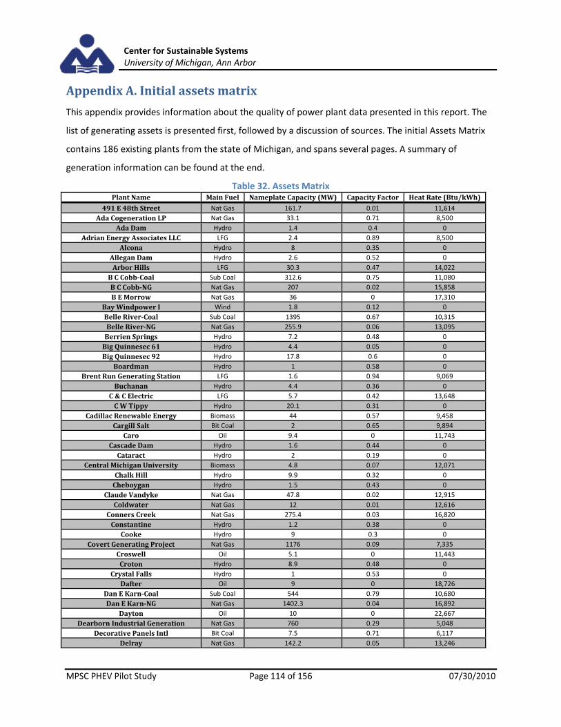
Center for Sustainable Systems University of Michigan, Ann Arbor
MPSC PHEV Pilot Study Page 114 of 156 07/30/2010
Appendix A. Initial assets matrix
This appendix provides information about the quality of power plant data presented in this report. The
list of generating assets is presented first, followed by a discussion of sources. The initial Assets Matrix
contains 186 existing plants from the state of Michigan, and spans several pages. A summary of
generation information can be found at the end.
Table 32. Assets Matrix Plant Name Main Fuel Nameplate Capacity (MW) Capacity Factor Heat Rate (Btu/kWh)
491 E 48th Street Nat Gas 161.7 0.01 11,614
Ada Cogeneration LP Nat Gas 33.1 0.71 8,500
Ada Dam Hydro 1.4 0.4 0
Adrian Energy Associates LLC LFG 2.4 0.89 8,500
Alcona Hydro 8 0.35 0
Allegan Dam Hydro 2.6 0.52 0
Arbor Hills LFG 30.3 0.47 14,022
B C Cobb‐Coal Sub Coal 312.6 0.75 11,080
B C Cobb‐NG Nat Gas 207 0.02 15,858
B E Morrow Nat Gas 36 0 17,310
Bay Windpower I Wind 1.8 0.12 0
Belle River‐Coal Sub Coal 1395 0.67 10,315
Belle River‐NG Nat Gas 255.9 0.06 13,095
Berrien Springs Hydro 7.2 0.48 0
Big Quinnesec 61 Hydro 4.4 0.05 0
Big Quinnesec 92 Hydro 17.8 0.6 0
Boardman Hydro 1 0.58 0
Brent Run Generating Station LFG 1.6 0.94 9,069
Buchanan Hydro 4.4 0.36 0
C & C Electric LFG 5.7 0.42 13,648
C W Tippy Hydro 20.1 0.31 0
Cadillac Renewable Energy Biomass 44 0.57 9,458
Cargill Salt Bit Coal 2 0.65 9,894
Caro Oil 9.4 0 11,743
Cascade Dam Hydro 1.6 0.44 0
Cataract Hydro 2 0.19 0
Central Michigan University Biomass 4.8 0.07 12,071
Chalk Hill Hydro 9.9 0.32 0
Cheboygan Hydro 1.5 0.43 0
Claude Vandyke Nat Gas 47.8 0.02 12,915
Coldwater Nat Gas 12 0.01 12,616
Conners Creek Nat Gas 275.4 0.03 16,820
Constantine Hydro 1.2 0.38 0
Cooke Hydro 9 0.3 0
Covert Generating Project Nat Gas 1176 0.09 7,335
Croswell Oil 5.1 0 11,443
Croton Hydro 8.9 0.48 0
Crystal Falls Hydro 1 0.53 0
Dafter Oil 9 0 18,726
Dan E Karn‐Coal Sub Coal 544 0.79 10,680
Dan E Karn‐NG Nat Gas 1402.3 0.04 16,892
Dayton Oil 10 0 22,667
Dearborn Industrial Generation Nat Gas 760 0.29 5,048
Decorative Panels Intl Bit Coal 7.5 0.71 6,117
Delray Nat Gas 142.2 0.05 13,246

Center for Sustainable Systems University of Michigan, Ann Arbor
MPSC PHEV Pilot Study Page 115 of 156 07/30/2010
Detour Oil 6 0.01 19,396
Diesel Plant NG Nat Gas 10 0 20,365
Diesel Plant Oil Oil 20.9 0.01 10,872
Donald C Cook Nuke 2285.3 0.87 0
DTE East China LLC Nat Gas 357.6 0.03 12,296
Eckert Station Sub Coal 375 0.46 13,764
Edenville Hydro 4.8 0.35 0
Edison Sault Hydro 41.8 0.58 0
Endicott Station Bit Coal 58.2 0.74 16,717
EQ Waste Energy Services LFG 1.4 0.81 8,500
Erickson Station Sub Coal 154.7 0.72 12,152
Escanaba Bit Coal 49.8 0.41 12,510
Escanaba Paper Company Biomass 103.3 0.76 14,353
Fermi Nuke 1281 0.78 2
Five Channels Hydro 6 0.42 0
Foote Hydro 9 0.34 0
Four Mile Hydropower Project Hydro 2 0.48 0
Frank Jenkins Nat Gas 3.8 0 8,357
French Landing Dam Hydro 1.6 0.44 0
French Paper Hydro Hydro 1.3 0.74 0
Gaylord 1 Nat Gas 80 0.02 16,784
Gaylord 2 Nat Gas 70.2 0.01 16,545
Genesee Power Station LP Biomass 39.5 0.68 16,643
George Johnson Nat Gas 73 0.05 11,711
Gladstone Oil 22.6 0.03 19,491
GM WFG Pontiac Site Power Plant Bit Coal 28.9 0 6,859
Grand Blanc Generating Station LFG 4 0.9 11,594
Grand Rapids Hydro 7.5 0.5 0
Granger Electric Generating Station #1 LFG 3.2 0.94 11,836
Granger Electric Generating Station #2 LFG 4 0.78 12,771
Graphic Packaging Oil 11.8 0.09 17,392
Grayling Generating Station Biomass 38 0.76 15,975
Greater Detroit Resource Recovery Biomass 68.4 0.44 7,050
Greenwood Nat Gas 1071.3 0.08 12,143
Hancock Nat Gas 160.2 0.01 13,382
Harbor Beach Bit Coal 125 0.33 10,658
Hardy Hydro 30 0.34 0
Hemlock Falls Hydro 3.1 0.33 0
Henry Station Nat Gas 15.4 0.01 8,997
Hillman Power LLC Biomass 20 0.77 15,812
Hillsdale Nat Gas 21.9 0.01 11,279
Hodenpyl Hydro 19 0.18 0
Hoist Hydro 4.4 0.32 0
Hydro Plant Hydro 2.2 0.36 0
J B Sims Bit Coal 65 0.77 10,390
J C Weadock Sub Coal 331.2 0.71 11,079
J H Campbell Sub Coal 1558.7 0.73 10,211
J R Whiting Sub Coal 364 0.73 11,765
James De Young Bit Coal 62.8 0.55 14,874
James R. Smith Hydro 3.2 0.4 0
Kalamazoo River Generating Station Nat Gas 73.1 0.02 13,945
Kalkaska CT #1 Nat Gas 75 0.01 11,102
Kent County Waste to Energy Facility Biomass 18 0.64 20,422
Kinder Morgan Power Jackson Facility Nat Gas 649 0.04 8,788
Kingsford Hydro 9 0.32 0
LaFarge Alpena Oil 47.2 0.68 9,659
Livingston Generating Station Nat Gas 170.1 0.01 16,000

Center for Sustainable Systems University of Michigan, Ann Arbor
MPSC PHEV Pilot Study Page 116 of 156 07/30/2010
Loud Hydro 4 0.47 0
Lowell Nat Gas 3.6 0.01 4,377
Ludington Hydro 1978.8 ‐0.1 0
Lyon Development LFG 5 0.46 17,491
Main Street Nat Gas 6 0 9,077
Manistique Oil 4.8 0.01 16,469
Marshall Nat Gas 11.8 0.01 10,763
McClure Hydro 8 0.48 0
Menominee Acquisition Bit Coal 4 0.21 8,066
Menominee Mill Marinette Hydro 1.8 0.95 0
Michigamme Falls Hydro 10.6 0.3 0
Michigan Power LP Nat Gas 154.1 0.78 8,476
Midland Cogeneration Venture Nat Gas 1853.8 0.38 7,289
Mio Hydro 5 0.3 0
Mistersky Nat Gas 189 0.15 14,955
Modular Power LLC Oil 14.8 0 10,745
Monroe Bit Coal 3293.1 0.65 9,436
Mottville Hydro 1.6 0.42 0
Neenah Paper Munising Mill Bit Coal 6.2 0.7 10,271
Newberry Oil 5.5 0.01 11,119
Ninth Street Hydropower Project Hydro 1.2 0.56 0
Northeast Nat Gas 129.8 0 15,592
Norway Hydro 5.6 0.45 0
Norway Point Hydropower Project Hydro 4 0.34 0
Otsego Mill Power Plant Nat Gas 21.2 0.46 9,454
Ottawa Generating Station LFG 4.8 0.94 11,165
Palisades Nuke 811.8 0.93 0
Parkedale Pharmaceuticals Nat Gas 2.8 0.9 14,783
Peavy Falls Hydro 15 0.34 0
Peoples Generating Station LFG 3.2 0.95 7,037
Pine Street Nat Gas 7 0 8,956
Pine Tree Acres LFG 5.6 0.97 10,686
Plant Four Oil 24 0.02 15,454
Portage Oil 22.6 0.08 16,570
Powertrain Warren General Motors Nat Gas 4 0.45 5,421
Presque Isle Bit Coal 624.7 0.63 11,815
Prickett Hydro 2.2 0.45 0
Putnam Oil 13.5 0 18,085
Quinnesec Mich Mill Biomass 28 0.86 14,106
Renaissance Power LLC Nat Gas 680 0.08 10,879
River Rouge‐Coal Sub Coal 650.6 0.52 9,589
River Rouge‐NG Nat Gas 282.6 0 9,957
Riverview Energy Systems LFG 6.6 0.62 10,886
Rogers Hydro 6.8 0.44 0
Romulus Operations Powertrain Nat Gas 10.7 0 40,790
S D Warren Muskegon Bit Coal 50.9 0.45 6,427
Saint Marys Falls Hydro 18.4 1.05 0
Sanford Hydro 3.6 0.23 0
Saxon Falls Hydro 1.2 1.05 0
Secord Hydro 1.2 0.33 0
Shiras Sub Coal 77.5 0.45 13,751
Smallwood Hydro 1.2 0.28 0
St Clair Sub Coal 1570.9 0.54 10,309
St Louis Oil 6.9 0.01 9,725
State St Generating Oil 16.2 0.01 8,499
Stone Container Ontonagon Mill Bit Coal 15.6 0.75 5,640
Straits Nat Gas 20 0.01 17,927

Center for Sustainable Systems University of Michigan, Ann Arbor
MPSC PHEV Pilot Study Page 117 of 156 07/30/2010
Sumpter Nat Gas 340 0.04 13,107
Sumpter Energy Associates LFG 12 0.83 14,189
Superior Falls Hydro 1.2 1.17 0
T B Simon Power Plant Bit Coal 99.3 0.28 6,618
TES Filer City Station Bit Coal 70 0.73 12,310
Thetford Nat Gas 222.4 0.02 17,327
Tower Oil 25.2 0 18,829
Trenton Channel Bit Coal 775.5 0.62 10,442
Twin Falls Hydro 7.6 0.47 0
Ubly Oil 12.4 0 19,219
University of Michigan Nat Gas 44.5 0.41 12,392
Venice Resources Gas Recovery LFG 1.6 0.66 15,890
Vestaburg Nat Gas 31.4 0.01 18,002
Victoria Hydro 12 0.49 0
Viking Energy of Lincoln Biomass 18 0.92 9,698
Viking Energy of McBain Biomass 18 0.88 13,743
Voss Lantz Nat Gas 1 0.47 8,500
Voss Taylor Nat Gas 1 0.43 8,500
Warner Lambert Nat Gas 12.4 0.24 8,500
Water Street Station Nat Gas 12.6 0.01 15,613
Way Dam Hydro 1.8 0.3 0
Webber Hydro 4.3 0.26 0
White Pine Electric Power Bit Coal 60 0.24 15,886
White Rapids Hydro 9.1 0.36 0
Wyandotte Bit Coal 78.4 0.46 14,812
Zeeland Nat Gas 22.3 0.01 13,658
Zeeland Plant Nat Gas 968.1 0.07 8,852
Table 33. Summary of Generation Details
Summary of Generation Details:
Sum of generation 121,328 GWh
Sum of generation excluding wind and hydro 120,999 GWh
2005 total electric demand 125,165 GWh
Imported percentage 3.33%
As noted previously in this report, the source for the initial set of power plants and their
generation details is the EPA’s eGRID database. The specific version of this database used was published
in 2007 and contains generation data for the year 2005. The information provided in eGRID includes fuel
consumption, emissions and emission rates, and generation and resource mix; along with plant
identification, location, and structural information for Michigan power plants. These eGRID files
represented the most comprehensive power generation data source for the purposes of this study.
However, certain data quality issues were identified within eGRID that required special attention. Some
of these disparities could be ameliorated from changes within the dataset itself while other
discrepancies necessitated input from separate sources. In addition to eGRID, values for certain
categories were derived from two principal sources: EIA 2005 906/920 electricity database files and the

Center for Sustainable Systems University of Michigan, Ann Arbor
MPSC PHEV Pilot Study Page 118 of 156 07/30/2010
[57]. The original eGRID database contained a total 193 plants. The final list of generating assets as
displayed above and utilized in this analysis totals 186. This procedure had 6 steps: (1) re‐labeling of
duplicate plants, (2) elimination of plants with capacity factor < zero, (3) correction of primary fuel type
discrepancies, (4) break‐out of specific plants to generator level detail, (5) correction of inconsistent
heat rates, and (6) substitution of irrational emission factors. Details for each step are defined in greater
detail as follows:
1. From the original set of eGRID data, there two separate plants that were both named ‘Diesel
Plant’ and two separate plants that were both named ‘Gaylord’. Both sets of duplicate plant
names were broken out into the following: Diesel Plant Oil, Diesel Plant NG, Gaylord 1 and
Gaylord 2. The total number of plants did not change; only plant names were altered.
2. All plants listed with negative capacity factors, aside from the Ludington pumped hydro unit,
were removed from the assets list. Eleven plants fit this description, all of which were small (in
terms of nameplate capacity) fossil fuel generators.
3. The ‘Fermi’ plant, confirmed by DTE Energy to be a nuclear generation unit, was listed in eGRID
as an oil plant. The primary fuel type for Fermi was changed to nuclear.
4. The eGRID workbook, for the year 2005, includes spreadsheets for boilers, generators and
plants. Information from the plant‐level sheet was used for the majority of the analysis.
However there were a few plants that required generator break‐outs based on the discrepancy
between the plants listed primary fuel type and percentage of plant generation from that fuel
type. Plants were broken down to generator unit level if they met the following criteria: (1) the
discrepancy just described was greater than one percent, (2) it was a fossil fuel plant that
provided at least one percent of the total power generation. If a plant met these criteria, it was
broken into generating units based on distinct fuel types. For example, Dan E. Karn is a plant
that is comprised of five generators, three natural gas and two coal generators. It is sufficiently
large in terms of generation, and therefore was split into two separate “plants” named Dan E.
Karn‐NG and Dan E. Karn‐Coal, with nameplate and capacity factors characterized by the
appropriate group of the generators. These steps were necessary for four plants in the model:
Dan E. Karn, B.C. Cobb, River Rouge and Belle River. Emissions and heat input for each fuel type
was calculated by mapping the boilers to the generating units within the eGRID workbook. This
step brings the total number of plants to 186.
5. Heat rate improvement measures were taken for fossil fuel assets whose heat rates were

Center for Sustainable Systems University of Michigan, Ann Arbor
MPSC PHEV Pilot Study Page 119 of 156 07/30/2010
greater than 17,000 or less than 9000 (in the case of coal) or less than 7000 (in the case of
natural gas or oil), deemed ‘unreasonable’. This was true of 34 plants in the database. The new
heat rates that were assigned to these plants came from the EIA‐906/920 electricity database
files for 2005.
6. Finally, there were two plants, Midland Cogeneration Venture and Dearborn Industrial
Generation, with unreasonably low NOX, SO2 and CO2 emission rates, rates near zero. These
values were corrected by substituting NOX and SO2 rates from MAERS and CO2 rates from EPRI
2007 TAG for next generation natural gas plants. CO2 rates for these plants could not be found in
either the MAERS or EIA 906/920 documents. The value from EPRIs TAG was deemed a prudent
choice as both of these plants a relatively new co‐generation units and therefore should
theoretically have lower CO2 emission rates compared to their conventional counterparts

Center for Sustainable Systems University of Michigan, Ann Arbor
MPSC PHEV Pilot Study Page 120 of 156 07/30/2010
Appendix B. Scripted fleet retirements and additions
Given the time span of this study, it is probable that plants in operation will not continue to provide
electricity for the entire twenty year span. This is due in part to the fact that plant efficiency decreases
with increasing age, a relationship excluded from the present model. Taking plants offline within the
model is termed ‘retirement,’, and two sets of retirement matrices are used in the model. Within the
baseline list are plants specified per the Michigan Capacity Need Forum – Report to the Michigan Public
Service Commission (Appendices) in 2006[26]. The accelerated retirements is based on the age of the
generation unit. Generator units of power plants are be retired once they reach the age 60. Tables of
both plant retirement schedules are below:
Table 34. Baseline retirements list Plant Name Year MW Plant Name Year MW Plant Name Year MW
B.C. Cobb‐NG 2013 68 Northeast 2018 124 B C Cobb‐Coal 2022 160
B.C. Cobb‐NG 2013 61 Northeast 2018 153 River Rouge‐Coal 2022 155
B.C. Cobb‐NG 2015 52 J R Whiting 2018 162 J C Weadock 2022 247
491 E 48th Street 2015 39 Eckert Station 2019 46 Wyandotte 2022 22
Trenton Channel 2015 210 St Clair 2019 171 Eckert Station 2023 47
Conners Creek 2016 11 St Clair 2019 158 Escanaba 2023 47
James De Young 2016 215 Presque Isle 2020 155 Mistersky 2023 280
J R Whiting 2017 102 J C Weadock 2020 25 River Rouge‐Coal 2023 26
J R Whiting 2017 102 B C Cobb‐Coal 2021 160 Dan E Karn‐Coal 2024 255
River Rouge‐NG 2021 242 Dan E Karn‐Coal 2024 260
Table 35. Accelerated Retirements list Plant Name Year MW Plant Name Year MW Plant Name Year MW
Trenton Channel 2010 120 J C Weadock 2015 156.3 Fermi 2026 16Trenton Channel 2010 120 Presque Isle 2015 25 Hancock 2026 41.8
Mistersky 2010 44 Dafter 2015 1 Northeast 2026 16Diesel Plant Oil 2010 2.7 Dafter 2015 1 Northeast 2026 16Diesel Plant Oil 2010 2.7 Dafter 2015 1 Northeast 2026 16
Hillsdale 2010 2.7 LaFarge Alpena 2015 10 Presque Isle 2026 57.8Marshall 2010 1 Lowell 2016 1.1 Main Street 2026 1.1Marshall 2010 1.7 B C Cobb‐Coal 2016 156.3 Main Street 2026 1.3Newberry 2010 0.7 River Rouge‐NG 2016 282.6 Zeeland 2026 1.4
Frank Jenkins 2010 0.8 Zeeland 2017 2 T B Simon Power 2026 12.5St Louis 2010 0.6 Decorative 2017 7.5 Stone Container 2026 15.6
Main Street 2010 0.9 B C Cobb‐Coal 2017 156.3 J H Campbell 2027 403.9Diesel Plant NG 2010 1 River Rouge‐Coal 2017 292.5 Hancock 2027 19Diesel Plant NG 2010 1 J C Weadock 2018 156.3 Hancock 2027 19Diesel Plant NG 2010 1 Escanaba 2018 11.5 Hancock 2027 19Diesel Plant NG 2010 1 Escanaba 2018 11.5 Harbor Beach 2027 2Wyandotte 2010 11.5 Mistersky 2018 50 Harbor Beach 2027 2
Tower 2010 1.3 Eckert Station 2018 44 Northeast 2027 16Tower 2010 1.3 St Louis 2018 1.3 Shiras 2027 12.5Caro 2010 1.3 Wyandotte 2018 22 Main Street 2027 0.6

Center for Sustainable Systems University of Michigan, Ann Arbor
MPSC PHEV Pilot Study Page 121 of 156 07/30/2010
Caro 2010 1.3 River Rouge‐Coal 2018 358.1 Zeeland 2027 1.1Ubly 2010 0.6 Vestaburg 2019 3 Claude Vandyke 2027 23Ubly 2010 0.7 Graphic 2019 10 B E Morrow 2028 18Ubly 2010 0.7 Dan E Karn‐Coal 2019 136 Gaylord 1 2028 16Ubly 2010 0.9 Dan E Karn‐Coal 2019 136 J H Campbell 2028 18.6
Vestaburg 2010 0.3 Manistique 2020 2 J C Weadock 2028 18.6Vestaburg 2010 0.7 Hillsdale 2020 4.1 J R Whiting 2028 18.6Vestaburg 2010 0.7 Eckert Station 2020 47 Harbor Beach 2028 121
B C Cobb‐NG 2010 69 Dafter 2020 3 St Clair 2028 18.5B C Cobb‐NG 2010 69 Dafter 2020 3 Trenton Channel 2028 535.5B C Cobb‐NG 2010 69 Vestaburg 2020 3 Eckert Station 2028 80S D Warren 2010 3.5 St Clair 2021 352.7 S D Warren 2028 19.1Menominee 2010 2.5 Main Street 2021 1 Cargill Salt 2028 2Neenah Paper 2010 6.2 Dan E Karn‐Coal 2021 136 B E Morrow 2029 18Conners Creek 2011 135 Dan E Karn‐Coal 2021 136 Straits 2029 20Conners Creek 2011 135 J H Campbell 2022 265.2 Hancock 2029 19.6James De Young 2011 11.5 Presque Isle 2022 37.5 Monroe 2029 2.7
St Louis 2011 0.9 James De Young 2022 22 Monroe 2029 2.7Tower 2011 1.3 Menominee 2022 1.5 Monroe 2029 2.7
J R Whiting 2012 106.3 Zeeland 2023 1.7 Monroe 2029 2.7J R Whiting 2012 106.3 Presque Isle 2024 54.4 Monroe 2029 2.7
Diesel Plant Oil 2012 5.5 Eckert Station 2024 80 St Clair 2029 544.5Caro 2012 1.3 Lowell 2025 1.1 Coldwater 2029 3.5
LaFarge Alpena 2012 12 T B Simon Power 2025 12.5 James De Young 2029 29.3J R Whiting 2013 132.8 Gaylord 1 2026 16 Wyandotte 2029 7.5St Clair 2013 168.7 Gaylord 1 2026 16 Pine Street 2029 1.1St Clair 2013 156.2 Gaylord 1 2026 16 Pine Street 2029 1.1Marshall 2013 1.1 Gaylord 1 2026 16 Escanaba Paper 2029 27.2St Clair 2014 156.2 Dayton 2026 2 Thetford 2030 33.6St Clair 2014 168.7 Dayton 2026 2 Thetford 2030 33.6
Diesel Plant Oil 2014 3 Dayton 2026 2 Thetford 2030 33.6Hillsdale 2014 3.5 Dayton 2026 2 Thetford 2030 33.6
Eckert Station 2014 44 Dayton 2026 2 Hancock 2030 41.8White Pine Electric 2014 20 Fermi 2026 16 St Clair 2030 2.7White Pine Electric 2014 20 Fermi 2026 16 St Clair 2030 2.7White Pine Electric 2014 20 Fermi 2026 16 Eckert Station 2030 80

Center for Sustainable Systems University of Michigan, Ann Arbor
MPSC PHEV Pilot Study Page 122 of 156 07/30/2010
In order to replace the capacity retired, new plants must built in accordance to the methodology in
subsection 3.3. Table 36 highlights their attributes.
Table 36. New Capacity Technology Characteristics
Capacity Factor
Availability Factor
NOX
emission rate
(lb/MWh)
SO2
emission rate
(lb/MWh)
CO2
emission rate
(lb/MWh)
CH4
emission rate
(lb/MWh)
N2O emission rate
(lb/MWh)
Heat Rate (Btu/kWh)
Coal 0.80 0.87 0.7075 0.1539 1922.81 21.995 32.336 8844
Oil 0.18 0.80 14.7 0.0147 1289.13 37.706 6.161 9800
Natural Gas 0.80 0.87 0.1285 0.00428 951.376 18.618 1.862 7139
Nuclear 0.90 0.90 ‐ ‐ ‐ ‐ ‐ 9502
Biomass 0.80 0.85 1.485 0.2997 0 102.171 13.623 10607
Wind 0.29 0.13 ‐ ‐ ‐ ‐ ‐ ‐
LFG 0.90 0.90 ‐ ‐ ‐ ‐ ‐ ‐

Center for Sustainable Systems University of Michigan, Ann Arbor
MPSC PHEV Pilot Study Page 123 of 156 07/30/2010
Appendix C. Future baseline consumer demand
To develop an hourly load profile from 2009‐2030, we used a scaled version of the load reported in
Michigan for 2008. The hourly load profile for 2008 was determined by summing up the reported
demand [37] for the following utilities:
‐ DTE Energy
‐ Consumers Energy
‐ Upper Peninsula Power Company
‐ Wolverine Power Cooperative
This demand profile was scaled to represent all Michigan utility sales based on data reported by
the MPSC for 2008 [58]. If sales data provided is summed, it reports 94,793,015 MWh sold by the four
utilities above and 105,475,262 MWh sold in Michigan. This disagrees slightly with the hourly load data
from FERC. If that is summed, the total load provided for by the four utilities was 97,159,607 MWh. To
determine the hourly load for all of Michigan, the FERC hourly load is multiplied by the ratio of total
Michigan sales to the sales in the listed utilities. This gives us a total of 108,108,546 MWh of load
satisfied in Michigan. The hourly values that sum up to this load will be what is used to extrapolate out
a forecast for Michigan growth assuming relative load profiles do not change from year to year.
The FERC filings and sales information represent the electricity demanded of the utilities in
Michigan by their customers, and thus do not include transmission and distribution losses in the system.
Approximately 9% of electricity generated is lost in its transmission and distribution from power plants
to end‐use consumers[59]. To turn this demand into a load at the generator, the base year demand is
multiplied by a factor of 1.09 to represent these losses.
To forecast Michigan load growth over the length of a simulation, two sources are used. First,
the EIA’s Annual Energy Outlook [60] provides forecasts of electricity usage and generation up until
2030. This is coupled with forecasts provided in FERC Form 714 filings by the 4 utilities mentioned,
which forecast out ten years from 2008 – 2018. To determine the annual percentage change in
electricity generation in Michigan. The forecasts for the four utilities are summed together to determine
an annual percentage growth rate for the state.
Where is the growth rate in MI for a given year, , and is the sum of electricity demand
forecasted by the four utilities for that year. The Michigan specific data only goes out to 2018, but

Center for Sustainable Systems University of Michigan, Ann Arbor
MPSC PHEV Pilot Study Page 124 of 156 07/30/2010
forecasts to 2030 are needed, so the rate of growth for the rest of the country is scaled to a Michigan
growth rate for the last 12 years. To do this we use the same equation with the forecasted national “net
generation available to the grid” to get a growth rate, rk, for the nation for every year to 2030. To scale
demand, we examine the ratios of expected national to Michigan yearly growth from 2009 to 2018 and
determine the average ratio, D.
10 10
This average ratio is then multiplied into the national electricity rate of change from years 2019‐
2030 to get a Michigan specific demand change for those years. This outputs a vector of yearly growth
factors for Michigan loads that can be coupled with the adjusted load from 2008 to forecast hourly load
profiles for every year between 2009 and 2030. Below is a graph showing the growth rates used. It
shows the EIA, the reported growth rates by MI Utilities, and the rates that were generated using the
calculations discussed.
Figure 60: Forecasted annual load growth rate for MI and the USA

Center for Sustainable Systems University of Michigan, Ann Arbor
MPSC PHEV Pilot Study Page 125 of 156 07/30/2010
Appendix D. Fuel prices for Economic Dispatch
While Figure 34 shows the fuel prices visually, fuel prices in dollars per mmBtu each year are presented
in the table below. Prices are in $/mmBtu for fuel costs (in 2008 dollars), and tax is $/metric ton CO2e.
Fuel prices are EIA predictions [39].
Table 37. Fuel costs used in the economic dispatch model
Sub‐bituminous Coal Bituminous Coal Oil Natural Gas CO2 tax
2009 2.15 2.15 14.24 4.14 0
2010 1.99 1.99 13.91 4.85 0
2011 1.98 1.98 14.06 5.82 0
2012 1.99 1.99 15.2 6.17 10.8
2013 1.99 1.99 16.21 5.94 11.34
2014 1.99 1.99 16.89 5.9 11.91
2015 2.01 2.01 17.36 6.08 12.5
2016 1.99 1.99 18.22 6.16 13.13
2017 2 2 18.88 6.17 13.78
2018 1.99 1.99 19.51 6.22 14.47
2019 1.99 1.99 19.92 6.29 15.19
2020 1.98 1.98 20.25 6.42 15.95
2021 1.98 1.98 20.4 6.52 16.75
2022 1.99 1.99 20.58 6.69 17.59
2023 1.99 1.99 20.89 6.74 18.47
2024 1.99 1.99 21.07 6.7 19.39
2025 1.99 1.99 21.35 6.75 20.36
2026 2 2 21.6 6.91 21.38
2027 2 2 21.83 7.05 22.45
2028 2.01 2.01 22.14 7.27 23.57
2029 2.02 2.02 22.54 7.51 24.75
2030 2.03 2.03 22.71 7.73 25.99

Center for Sustainable Systems University of Michigan, Ann Arbor
MPSC PHEV Pilot Study Page 126 of 156 07/30/2010
Appendix E. Vehicle size class mapping
Within the PECM and MEFEM models, vehicles are handled by size class. The size classes used are
subcompact, compact, midsize, and large ‘car classes’, as well as the van, SUV, and pickup ‘truck classes.’
While this nomenclature is consistent through the model, in developing various parameters different
naming schema were used by different sources. In this appendix, the names used to create the
parameters within the original sources are mapped to the size classes used in the model.
Table 38. List of parameters and sources for mapping size classes Parameter Source
Trip Data for PECM 2009 NHTS[14]
Initial Vehicles Sales MI Motor Vehicle Registrations[22]
% of new vehicle sales AEO 2009[20]
New Conventional equivalent fuel economy (mpg) AEO 2009[20]
Table 39. Mapping size classes to source classes
Size Class Trip Data Initial Vehicle Sales % new Vehicle sales New CV equivalent mpg
Subcompact Car 40% of 2 door Subcompact Subcompact
Compact Car 60% of 2 door Compact Compact
Midsize Car 75% of 4 door, roadster Midsize Midsize
Large Car 25% of 4 door, roadster Large Large
Van Van Van Small/Large Van Small/Large Van
SUV SUV Station Wagon Small/Large Utility Small/Large Utility
Pickup Pickup Pickup Small/Large Pickup Small/Large Pickup

Center for Sustainable Systems University of Michigan, Ann Arbor
MPSC PHEV Pilot Study Page 127 of 156 07/30/2010
Appendix F. Plug‐in electric hybrid vehicle characteristics
Table 40. PHEV energy consumption rates for all size classes
Charge Depleting Electricity consumption
(kWh/mi)
Charge Sustaining Gasoline consumption
(mpg)
PHEV
Subcompact 0.240 50
Compact 0.246 43.5
Midsize 0.274 32.8
Large 0.3 26
Van 0.346 26.14
SUV 0.330 26.14
Pickup 0.372 21
Within the PECM model, plug‐in hybrids complete daily trips using some combination of electricity
stored in the battery and gasoline combustion. The consumption parameters used in the model vary by
size class and are listed in the table above. This appendix lists consumption parameters based on OEM
press releases and academic sources used to compile the table above. Typically for a size class, an
average of all electricity consumption parameters were taken, and a 55/45% city highway inverse
average for 2009 model year hybrids was used to find gasoline consumption parameters. However, as
data was sometimes unavailable, this is not the case for all size classes. Note that EV range and usable
battery size are listed for reference, and was not available for many academic sources.
Subcompact
A pre‐production electric vehicle, plug‐in electric hybrid, and a hybrid electric vehicle were
reviewed. The plug‐ins report similar charge depleting electricity consumptions, whereas there is a large
difference between the charge sustaining gasoline consumption parameters, and an inverse average
was taken.

Center for Sustainable Systems University of Michigan, Ann Arbor
MPSC PHEV Pilot Study Page 128 of 156 07/30/2010
Table 41. Subcompact PHEV characteristics
EV Range (miles)
Usable Battery (kWh)
Charge Depleting electricity consumption
(kWh/mi)
Charge Sustaining Gasoline consumption
(mpg)
OEM
Mitsubishi i‐MiEV
60 16 0.24 ‐‐
Audi A1 e‐tron plug‐in
30 7.2 0.24 39.2
Honda Fit Hybrid
70
Compact
Two pre‐production plug in sources were used, as well as parameters from the Electric Power
Research Institute’s (EPRI’s) Hybrid Electric Working Group [Duvall, 2002, 2003, and 2004], to obtain the
electric charge depleting parameter used in the model. The charge sustaining fuel economy rating was
determined through a 55%/45% comparison of compact hybrids.
Table 42. Compact PHEV characteristics
EV Range (miles)
Usable Battery (kWh)
Charge Depleting electricity consumption
(kWh/mi)
Charge Sustaining Gasoline consumption (city/hwy
mpg)
OEM
Toyota Plug‐in Prius
15 3.64 0.243
VW Golf 93 21.2 0.228
Toyota Prius Hybrid
48/45
Honda Civic Hybrid
40/45
Honda Insight Hybrid
40/43
Academ
ic
EPRI [6] 33 8.6 0.260

Center for Sustainable Systems University of Michigan, Ann Arbor
MPSC PHEV Pilot Study Page 129 of 156 07/30/2010
Midsize
The midsize class electric consumption was determined from two pre production vehicles
characteristics as well as many academic references. Fuel consumption was determined from a
55%/45% split of hybrid vehicles in that class.
Table 43. Midsize PHEV characteristics
EV
Range (miles)
Usable Battery (kWh)
Charge Depleting electricity consumption (kWh/mi)
Charge Sustaining Gasoline
consumption (city/hwy mpg)
OEM
Chevy Volt 40 10.4 0.26
Fisker Karma
50 13.5 0.27
Ford Fusion Hybrid
36/41
Chevy Malibu Hybrid
26/34
Nissan Altima Hybrid
35/33
Toyota Camry Hybrid
33/34
Saturn Aura Hybrid
24/32
Academic
[6] 33 9.9 0.30
[3] 10 3.6 0.22
[3] 30 8.2 0.24
[3] 60 16.5 0.28
[61] 20 4.8 0.24
[62] 0.25
[63] 0.25
Large car
At the time of writing, there were no pre‐production plans for large passenger car sized PHEV or
EV, and the fuel consumption parameters were estimated to be larger than the Midsize class, but

Center for Sustainable Systems University of Michigan, Ann Arbor
MPSC PHEV Pilot Study Page 130 of 156 07/30/2010
smaller than any of the truck classes.
Van
Two vans, a passenger and a cargo van were examined to determine electric consumption. Note
that the Sprinter Van used a NiMH battery, and a general estimation comparable of Li‐Ion consumption,
based on Prius NiMH and Li‐Ion conversion characteristics. The SUV charge sustaining gasoline
consumption was used.
Table 44. Van PHEV characteristics
EV Range (miles)
Usable Battery (kWh)
Charge Depleting electricity consumption
(kWh/mi)
Charge Sustaining Gasoline consumption (city/hwy
mpg)
OEM
Luxgen MPV EV
120 miles 41.5 0.345
Daimler Sprinter
18.6 miles 9.8 0.346
SUV
The SUV size class within the model encompasses full size, midsize, and small/compact SUV, and
as such within the group the actual consumption parameters may vary. While the Ford Escape PHEV is
off‐schedule for production, specifications for the test models were used. Also, two publications
investigated the consumption parameters for various SUV sizes. Seven hybrid SUV of various sizes were
also viewed for the gasoline consumption parameter.
Table 45. SUV PHEV characteristics
EV Range (miles)
Usable Battery (kWh)
Charge Depleting electricity consumption
(kWh/mi)
Charge Sustaining Gasoline consumption
(city/hwy mpg)
OEM
Ford Escape PHEV
30 7.2 0.20
Ford Escape Hybrid
34/31
Toyota Highlander Hybrid
27/25
Chevy Tahoe Hybrid
21/22
Cadillac Escalade
20/21

Center for Sustainable Systems University of Michigan, Ann Arbor
MPSC PHEV Pilot Study Page 131 of 156 07/30/2010
Hybrid
Mercury Mariner Hybrid
34/31
Saturn Vue Hybrid
25/32
GMC Yukon Hybrid
21/22
Academ
ic
[6] (Midsize SUV)
33 12.5 0.38
[6] (Fullsize SUV)
33 15.2 0.46
[3] (Crossover SUV)
0.28
[3] (Midsize SUV)
0.33
Pickup
There are no current production pickups planned at the time the report was written. Fuel
consumption parameters for a converted F‐150, as well as one academic source were used. Five hybrids
were examined to estimate PHEV gasoline fuel economy.
Table 46. Pickup PHEV characteristics
EV Range (miles)
Usable Battery (kWh)
Charge Depleting electricity consumption
(kWh/mi)
Charge Sustaining Gasoline consumption
(city/hwy mpg)
OEM
Ford F‐150 Converted by
Enviva 38 12 0.316
[63] 0.429
Chevy Silverado Hybrid (2WD)
21/22
Chevy Silverado Hybrid (4WD)
20/20
GMC Sierra hybrid
21/22
Dodge Durango hybrid
20/22
Chrysler Aspen Hybrid
20/22
Table 47. Source list for PHEV characteristics

Center for Sustainable Systems University of Michigan, Ann Arbor
MPSC PHEV Pilot Study Page 132 of 156 07/30/2010
Hybrid fuel economies
http://www.fueleconomy.gov/
Plug in specifications
Mitsubishi i‐MiEV
http://www.mitsubishi‐motors.com/special/ev/index.html
Audi A1 e‐tron http://www.audi.com/com/brand/en/experience/audi_e‐tron/audi_a1_e‐
tron.tab_0002.html
Toyota Plug‐in Prius
http://www2.toyota.co.jp/en/news/09/12/1214.html
VW Golf Plug‐in http://www.autoweek.com/article/20100503/GREEN/100509981
Chevy Volt http://www.chevrolet.com/pages/open/default/future/volt.do
Fisker Karma http://www.fiskerautomotive.com/
Luxgen MPV EV http://www.luxgen‐motor.com/cars/EV/
Daimler Sprinter PHEV
http://www.calcars.org/calcars‐news/83.html (repost of press release from former daimlerchrysler)
Ford Escape PHEV
http://media.ford.com/article_display.cfm?article_id=27333
Ford F‐150 Converted by
Enviva
http://www.prlog.org/10119559‐envia‐announces‐rev‐plug‐in‐ford‐series‐truck‐conversion‐gets‐43‐mpg‐plug‐in‐your‐tru.html

Center for Sustainable Systems University of Michigan, Ann Arbor
MPSC PHEV Pilot Study Page 133 of 156 07/30/2010
Appendix G. Emissions allocation example from MEFEM
Subsection 3.5.3 showed in simple terms how the emissions from the electricity generation sector are
allocated to the transportation sector to account for PHEV charging. Within the model, changes to the
generation mix also play a role, and this appendix describes how marginal and average allocation
methods are affected by changes in the grid.
Table 48. Changes in baseline scenario generation (MWh) from 2009 to 2030
From Existing From New Total
Sub‐bituminous (14,045,042.73) 2,330,605.32 (11,714,437.41)
Bituminous (4,449,801.63) ‐ (4,449,801.63)
Oil (24,279.75) ‐ (24,279.75)
Natural gas (3,156,053.42) 3,529,202.34 373,148.93
Nuclear 0.00 524,386.20 524,386.20
Biomass (105,627.45) 1,055,558.80 949,931.35
Hydro (190.00) ‐ (190.00)
Wind (0.00) 18,400,759.89 18,400,759.89
LFG 0.00 1,359,369.85 1,359,369.85
(21,780,994.97) 27,199,882.40 5,418,887.43
Table 48 outlines the changes in the grid from 2009 to 2030 for the no PHEV, baseline simulation
by generation. Overall, the amount of electricity needed to be generated increased by 5,400 GWh, but
the current existing plants provide roughly 22,000 GWh less electricity to meet demand, with the
greatest reductions coming from coal generation, probably due to retirements in the system. New
capacity is added in many fuel types, however overall in the system coal and oil is reduced, while natural
gas, nuclear, biomass and wind generation is increased. The 190 MWh reduction of hydro is an artifact
of system dispatch, and changes slightly from year to year‐ hydro generation is neither reduced nor
added in the system. Note that all new coal is assumed sub‐bituminous.
Table 49 shows the average emissions factors for 2030 generation by fuel type. It can be seen
that oil has very high factors, but it comprises a very small proportion of generation. Aside from oil, and
that natural gas has high SOX factors, coal remains the highest pollutant per generation in the
categories. Existing biomass also has high NOX factors. While all new coal is assumed to be sub‐
bituminous, it can be seen that the emissions do not vary significantly between the two coal types.
Hydro and wind generation do not have emissions factors.
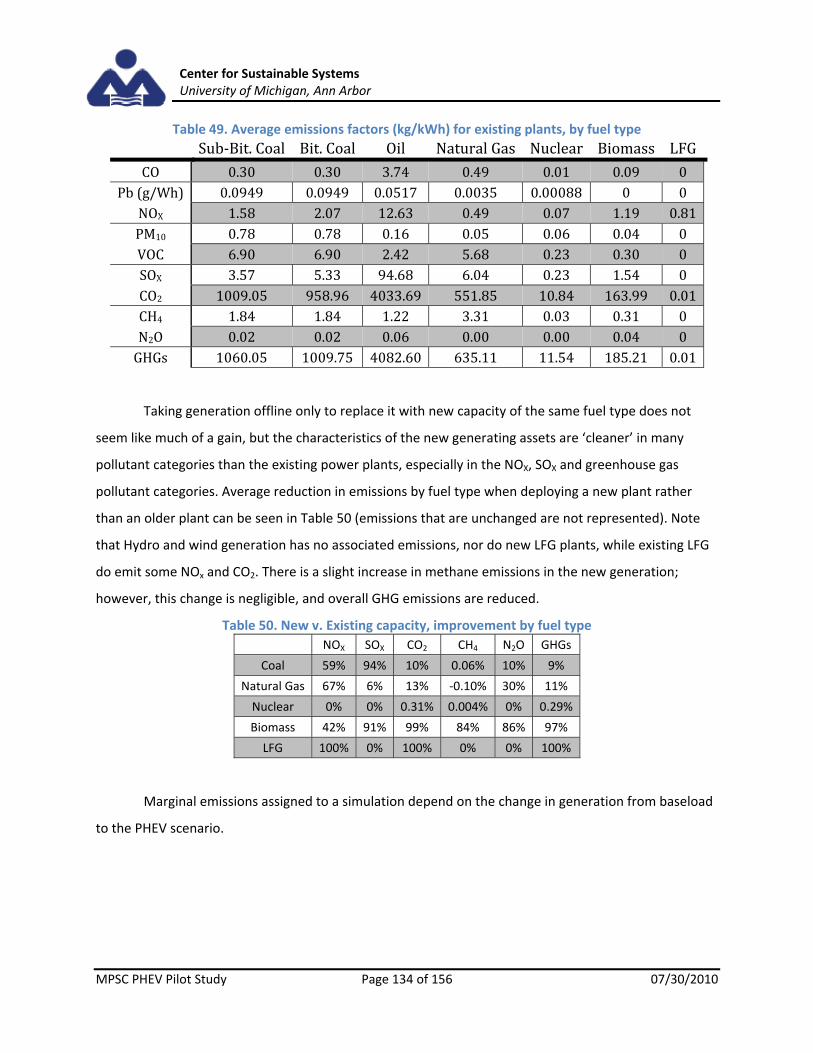
Center for Sustainable Systems University of Michigan, Ann Arbor
MPSC PHEV Pilot Study Page 134 of 156 07/30/2010
Table 49. Average emissions factors (kg/kWh) for existing plants, by fuel type
Sub‐Bit. Coal Bit. Coal Oil Natural Gas Nuclear Biomass LFG
CO 0.30 0.30 3.74 0.49 0.01 0.09 0
Pb (g/Wh) 0.0949 0.0949 0.0517 0.0035 0.00088 0 0
NOX 1.58 2.07 12.63 0.49 0.07 1.19 0.81
PM10 0.78 0.78 0.16 0.05 0.06 0.04 0
VOC 6.90 6.90 2.42 5.68 0.23 0.30 0
SOX 3.57 5.33 94.68 6.04 0.23 1.54 0
CO2 1009.05 958.96 4033.69 551.85 10.84 163.99 0.01
CH4 1.84 1.84 1.22 3.31 0.03 0.31 0
N2O 0.02 0.02 0.06 0.00 0.00 0.04 0
GHGs 1060.05 1009.75 4082.60 635.11 11.54 185.21 0.01
Taking generation offline only to replace it with new capacity of the same fuel type does not
seem like much of a gain, but the characteristics of the new generating assets are ‘cleaner’ in many
pollutant categories than the existing power plants, especially in the NOX, SOX and greenhouse gas
pollutant categories. Average reduction in emissions by fuel type when deploying a new plant rather
than an older plant can be seen in Table 50 (emissions that are unchanged are not represented). Note
that Hydro and wind generation has no associated emissions, nor do new LFG plants, while existing LFG
do emit some NOx and CO2. There is a slight increase in methane emissions in the new generation;
however, this change is negligible, and overall GHG emissions are reduced.
Table 50. New v. Existing capacity, improvement by fuel type
NOX SOX CO2 CH4 N2O GHGs
Coal 59% 94% 10% 0.06% 10% 9%
Natural Gas 67% 6% 13% ‐0.10% 30% 11%
Nuclear 0% 0% 0.31% 0.004% 0% 0.29%
Biomass 42% 91% 99% 84% 86% 97%
LFG 100% 0% 100% 0% 0% 100%
Marginal emissions assigned to a simulation depend on the change in generation from baseload
to the PHEV scenario.

Center for Sustainable Systems University of Michigan, Ann Arbor
MPSC PHEV Pilot Study Page 135 of 156 07/30/2010
Figure 61.Load duration curves with power bands, 2030 (EG1, CH1, FI1 & FI4)
The above figure shows the stacking dispatch results for the FI4 and FI1, base generation case
scenarios. It can be seen that much of the new load is served by a growth in the number of new plants.
The next table shows for the year 2030 the difference in generation by fuel type between the base case
and the high fleet infiltration scenario.
Table 51. Change in generation (MWh) from base case to FI4 (High PHEV) in 2030
From Existing From New Total
Sub‐bituminous (690,971.48) 3,405,526.55 2,714,555.07
Bituminous (990,491.16) ‐ (990,491.16)
Oil (10,827.32) ‐ (10,827.32)
Natural gas (289,119.70) 5,156,940.21 4,867,820.51
Nuclear 0.00 766,243.47 766,243.47
Biomass (45,669.97) 121,215.68 75,545.71
Hydro 0.00 ‐ 0.00
Wind ‐ 1,306,175.47 1,306,175.47
LFG (0.00) 565,150.39 565,150.39
TOTAL (2,027,079.63) 11,321,251.79 9,294,172.16
The above table shows that adding PHEV necessitates an increase of about 9,300GWh in the
base scenario. This is met by decreasing the use of existing plants and increasing the use of plants added
through capacity or renewable needs. Also, the majority of the new generation is done by natural gas
plants, although coal and wind do contribute as well. Again taking into account that Natural gas is
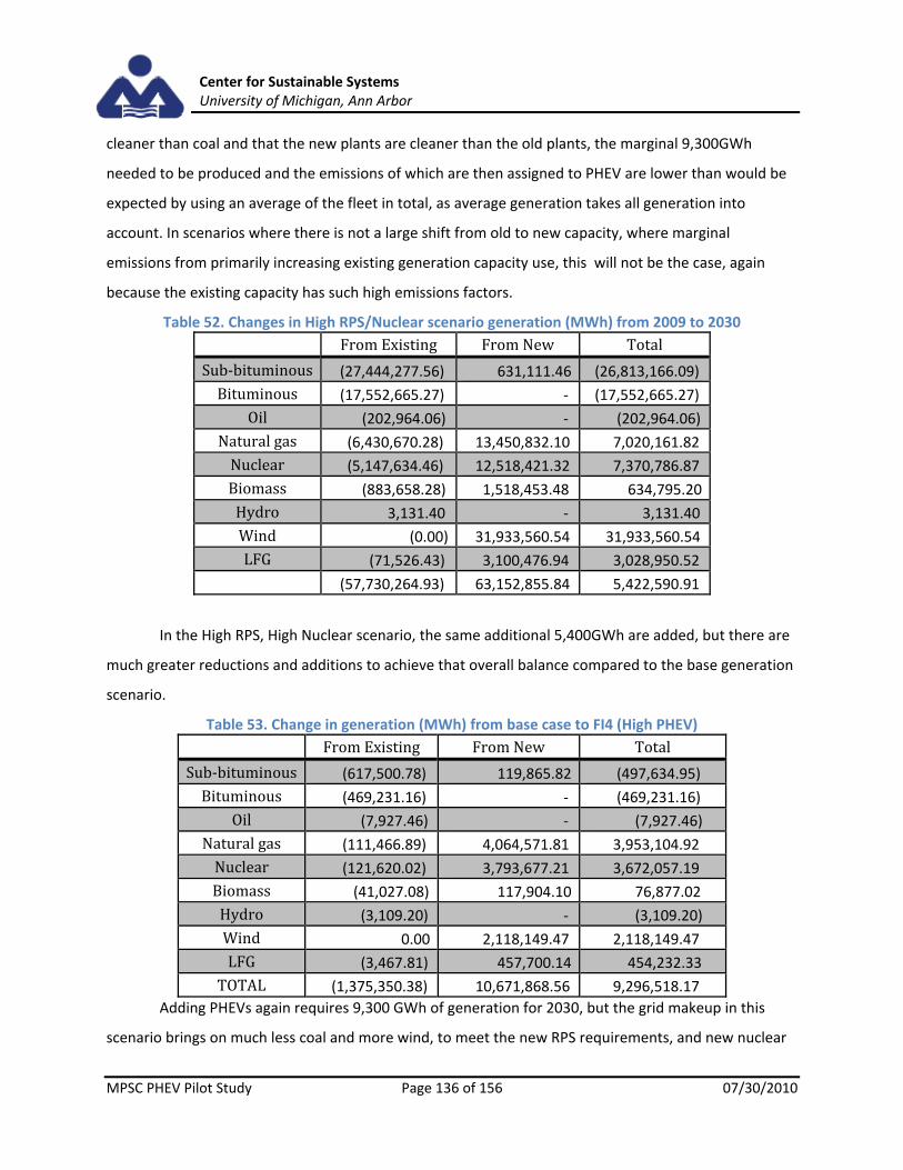
Center for Sustainable Systems University of Michigan, Ann Arbor
MPSC PHEV Pilot Study Page 136 of 156 07/30/2010
cleaner than coal and that the new plants are cleaner than the old plants, the marginal 9,300GWh
needed to be produced and the emissions of which are then assigned to PHEV are lower than would be
expected by using an average of the fleet in total, as average generation takes all generation into
account. In scenarios where there is not a large shift from old to new capacity, where marginal
emissions from primarily increasing existing generation capacity use, this will not be the case, again
because the existing capacity has such high emissions factors.
Table 52. Changes in High RPS/Nuclear scenario generation (MWh) from 2009 to 2030
From Existing From New Total
Sub‐bituminous (27,444,277.56) 631,111.46 (26,813,166.09)
Bituminous (17,552,665.27) ‐ (17,552,665.27)
Oil (202,964.06) ‐ (202,964.06)
Natural gas (6,430,670.28) 13,450,832.10 7,020,161.82
Nuclear (5,147,634.46) 12,518,421.32 7,370,786.87
Biomass (883,658.28) 1,518,453.48 634,795.20
Hydro 3,131.40 ‐ 3,131.40
Wind (0.00) 31,933,560.54 31,933,560.54
LFG (71,526.43) 3,100,476.94 3,028,950.52
(57,730,264.93) 63,152,855.84 5,422,590.91
In the High RPS, High Nuclear scenario, the same additional 5,400GWh are added, but there are
much greater reductions and additions to achieve that overall balance compared to the base generation
scenario.
Table 53. Change in generation (MWh) from base case to FI4 (High PHEV)
From Existing From New Total
Sub‐bituminous (617,500.78) 119,865.82 (497,634.95)
Bituminous (469,231.16) ‐ (469,231.16)
Oil (7,927.46) ‐ (7,927.46)
Natural gas (111,466.89) 4,064,571.81 3,953,104.92
Nuclear (121,620.02) 3,793,677.21 3,672,057.19
Biomass (41,027.08) 117,904.10 76,877.02
Hydro (3,109.20) ‐ (3,109.20)
Wind 0.00 2,118,149.47 2,118,149.47
LFG (3,467.81) 457,700.14 454,232.33
TOTAL (1,375,350.38) 10,671,868.56 9,296,518.17
Adding PHEVs again requires 9,300 GWh of generation for 2030, but the grid makeup in this
scenario brings on much less coal and more wind, to meet the new RPS requirements, and new nuclear

Center for Sustainable Systems University of Michigan, Ann Arbor
MPSC PHEV Pilot Study Page 137 of 156 07/30/2010
generation in place of coal. This would result in even lower marginal emissions, stemming from new
natural gas, nuclear, and wind, while even with the accelerated retirements, existing coal plants still
provide about a quarter of the total generation within the state, skewing the average.

Center for Sustainable Systems University of Michigan, Ann Arbor
MPSC PHEV Pilot Study Page 138 of 156 07/30/2010
Appendix H. Additional PECM Results
The PHEV energy consumption model (PECM) is a standalone model that analyzes the trip data within
the NHTS and simulates PHEV driving and charging. While certain scenarios and results were presented
in the main document, additional results specific to PECM are presented here.
Effect of Battery size
As the battery size increased, the electricity demand also increased. This also had the effect of ‘shifting’
the peak usage hour later and later, although the power at any given hour was increased as battery size
increased.
Figure 62. Effect of battery size on normalized PHEV charging load
Electricity use and percentage of electric miles increased as battery size increased, although the
relationship was non‐linear. Charging speed was shown to have a greater effect on these parameters as
battery size increased.
12:00 AM 4:00 AM 8:00 AM 12:00 PM 4:00 PM 8:00 PM 12:00 AM0
0.2
0.4
0.6
0.8
1
1.2
1.4
Hours of the Day
Electrical Load [MWh/h]
Increasing
battery size

Center for Sustainable Systems University of Michigan, Ann Arbor
MPSC PHEV Pilot Study Page 139 of 156 07/30/2010
Figure 63. Battery size effect on electricity consumption and percent of electric miles
Effect of Size class
Within PECM and MEFEM, there are seven vehicle size classes: sub‐compact, compact, midsize, large,
van, SUV, and pickup. Each of these classes have different associated parameters for consumption, and
while the sub‐compact, compact, midsize, and large car classes share NHTS trip data, the van, SUV, and
pickup classes each have a separate NHTS dataset. Appendix E shows the datasets used for each size
class.
The following figures are a daily and a weekly load curve with all seven size classes represented.
The larger classes, van, SUV, and pickup, typically draw more power. The car classes have similar curves
due to the shared data set, while the van class is noticeably more jagged, as the van data subset was the
smallest.
2 4 6 8 10 12 14 162
4
6
8
10
12
Useable Battery Size [kWh]
Electricity use [kW
h]
Electricity use for a Midsize vs. Battery Size
8A/120V Charging
12A/120V Charging
16A/240V Charging
2 4 6 8 10 12 14 160
20
40
60
80
Usable Battery Size [kWh]
Electric M
iles Percentage [%
] Percent of Miles Driven Electrically for a Midsize vs. Battery Size
8A/120V Charging
12A/120V Charging
16A/240V Charging
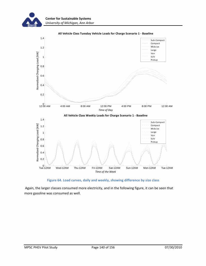
Center for Sustainable Systems University of Michigan, Ann Arbor
MPSC PHEV Pilot Study Page 140 of 156 07/30/2010
Figure 64. Load curves, daily and weekly, showing difference by size class
Again, the larger classes consumed more electricity, and in the following figure, it can be seen that
more gasoline was consumed as well.
12:00 AM 4:00 AM 8:00 AM 12:00 PM 4:00 PM 8:00 PM 12:00 AM0
0.2
0.4
0.6
0.8
1
1.2
1.4
Time of Day
Norm
alized
Charging Load [kW
]
All Vehicle Class Tuesday Vehicle Loads for Charge Scenario 1 ‐ Baseline
Sub‐Compact
Compact
Mids ize
Large
Van
SUV
Pickup
Tue-12AM Wed-12AM Thu-12AM Fri-12AM Sat-12AM Sun-12AM Mon-12AM Tue-12AM0
0.2
0.4
0.6
0.8
1
1.2
1.4
Time of the Week
Norm
alized
Charging Load [kW
]
All Vehicle Class Weekly Loads for Charge Scenario 1 ‐ Baseline
Sub‐Compact
Compact
Mids ize
Large
Van
SUV
Pickup

Center for Sustainable Systems University of Michigan, Ann Arbor
MPSC PHEV Pilot Study Page 141 of 156 07/30/2010
Figure 65. Energy consumption per week by size class
The smaller car size classes had a greater proportion of electrically driven miles, but for all
vehicle size classes ranged between 50 to 60%.
Figure 66. Percent of miles driven electrically by vehicle size class in the baseline charging scenario
Sub-Compact Compact Midsize Large Van SUV Pickup0
20
40
60Electricity Consumption by Vehicle Class for Charge Scenario 1 ‐ Baseline
Vehicle Size Class
Electricity Delivered
[kW
h]
Sub-Compact Compact Midsize Large Van SUV Pickup0
2
4
6
8Gasoline Consumption by Vehicle Class for Charge Scenario 1 ‐ Baseline
Vehicle Size Class
Gasoline Consumed
[gallons]
Sub-Compact Compact Midsize Large Van SUV Pickup0
20
40
60
80
100Percent of Miles Driven by Vehicle Class for Charge Scenario 1 ‐ Baseline
Vehicle Size Class
Driven M
ile Percent [%
]
Electric
Gasol ine

Center for Sustainable Systems University of Michigan, Ann Arbor
MPSC PHEV Pilot Study Page 142 of 156 07/30/2010
Additional Load lineups
While the loads are shown in Figure 42 overlaid on a July day’s demand, each scenario is reproduced
here with the normalized load, and the resulting load for high PHEV infiltration overlaid on a January
and July demand.
Figure 67. Baseline charging load profiles (High PHEV infiltration, 2030)
12:00 AM 4:00 AM 8:00 AM 12:00 PM 4:00 PM 8:00 PM 12:00 AM0
0.5
1
Tuesday Normalized Vehicle Load in Charge Scenario 1 ‐ Baseline
Time of Day
Charging Load [kW
]
12:00 AM 4:00 AM 8:00 AM 12:00 PM 4:00 PM 8:00 PM 12:00 AM0
1
2
3x 10
4 Electrical Loads for a July Tuesday in 2030 ‐ Charge Scenario 1 ‐ Baseline
Electrical Load [MWh/h]
Hours of the day
Non‐PHEV
PHEV
12:00 AM 4:00 AM 8:00 AM 12:00 PM 4:00 PM 8:00 PM 12:00 AM0
0.5
1
1.5
2x 10
4 Electrical Loads for a January Tuesday in 2030 ‐ Charge Scenario 1 ‐ Baseline
Electrical Load [MWh/h]
Hours of the day
Non‐PHEV
PHEV

Center for Sustainable Systems University of Michigan, Ann Arbor
MPSC PHEV Pilot Study Page 143 of 156 07/30/2010
Figure 68. Last minute charging load profiles (High PHEV infiltration, 2030)
12:00 AM 4:00 AM 8:00 AM 12:00 PM 4:00 PM 8:00 PM 12:00 AM0
0.5
1
Tuesday Normalized Vehicle Load in Charge Scenario 2 ‐ Last‐minute
Time of Day
Charging Load [kW
]
12:00 AM 4:00 AM 8:00 AM 12:00 PM 4:00 PM 8:00 PM 12:00 AM0
1
2
3x 10
4 Electrical Loads for a July Tuesday in 2030 ‐ Charge Scenario 2 ‐ Last‐minute
Electrical Load [MWh/h]
Hours of the day
Non‐PHEV
PHEV
12:00 AM 4:00 AM 8:00 AM 12:00 PM 4:00 PM 8:00 PM 12:00 AM0
0.5
1
1.5
2x 10
4 Electrical Loads for a January Tuesday in 2030 ‐ Charge Scenario 2 ‐ Last‐minute
Electrical Load [MWh/h]
Hours of the day
Non‐PHEV
PHEV

Center for Sustainable Systems University of Michigan, Ann Arbor
MPSC PHEV Pilot Study Page 144 of 156 07/30/2010
Figure 69. Home‐work charging load profiles (High PHEV infiltration, 2030)
12:00 AM 4:00 AM 8:00 AM 12:00 PM 4:00 PM 8:00 PM 12:00 AM0
0.5
1
Tuesday Normalized Vehicle Load in Charge Scenario 3 ‐ Home‐Work
Time of Day
Charging Load [kW
]
12:00 AM 4:00 AM 8:00 AM 12:00 PM 4:00 PM 8:00 PM 12:00 AM0
1
2
3x 10
4 Electrical Loads for a July Tuesday in 2030 ‐ Charge Scenario 3 ‐ Home‐Work
Electrical Load [MWh/h]
Hours of the day
Non‐PHEV
PHEV
12:00 AM 4:00 AM 8:00 AM 12:00 PM 4:00 PM 8:00 PM 12:00 AM0
0.5
1
1.5
2x 10
4 Electrical Loads for a January Tuesday in 2030 ‐ Charge Scenario 3 ‐ Home‐Work
Electrical Load [MWh/h]
Hours of the day
Non‐PHEV
PHEV

Center for Sustainable Systems University of Michigan, Ann Arbor
MPSC PHEV Pilot Study Page 145 of 156 07/30/2010
Figure 70. No‐charge window charging load profiles (High PHEV infiltration, 2030)
12:00 AM 4:00 AM 8:00 AM 12:00 PM 4:00 PM 8:00 PM 12:00 AM0
0.5
1
Tuesday Normalized Vehicle Load in Charge Scenario 4 ‐ No‐Charge Window
Time of Day
Charging Load [kW
]
12:00 AM 4:00 AM 8:00 AM 12:00 PM 4:00 PM 8:00 PM 12:00 AM0
1
2
3x 10
4Electrical Loads for a July Tuesday in 2030 ‐ Charge Scenario 4 ‐ No‐Charge Window
Electrical Load [MWh/h]
Hours of the day
Non‐PHEV
PHEV
12:00 AM 4:00 AM 8:00 AM 12:00 PM 4:00 PM 8:00 PM 12:00 AM0
0.5
1
1.5
2x 10
4Electrical Loads for a January Tuesday in 2030 ‐ Charge Scenario 4 ‐ No‐Charge Window
Electrical Load [MWh/h]
Hours of the day
Non‐PHEV
PHEV
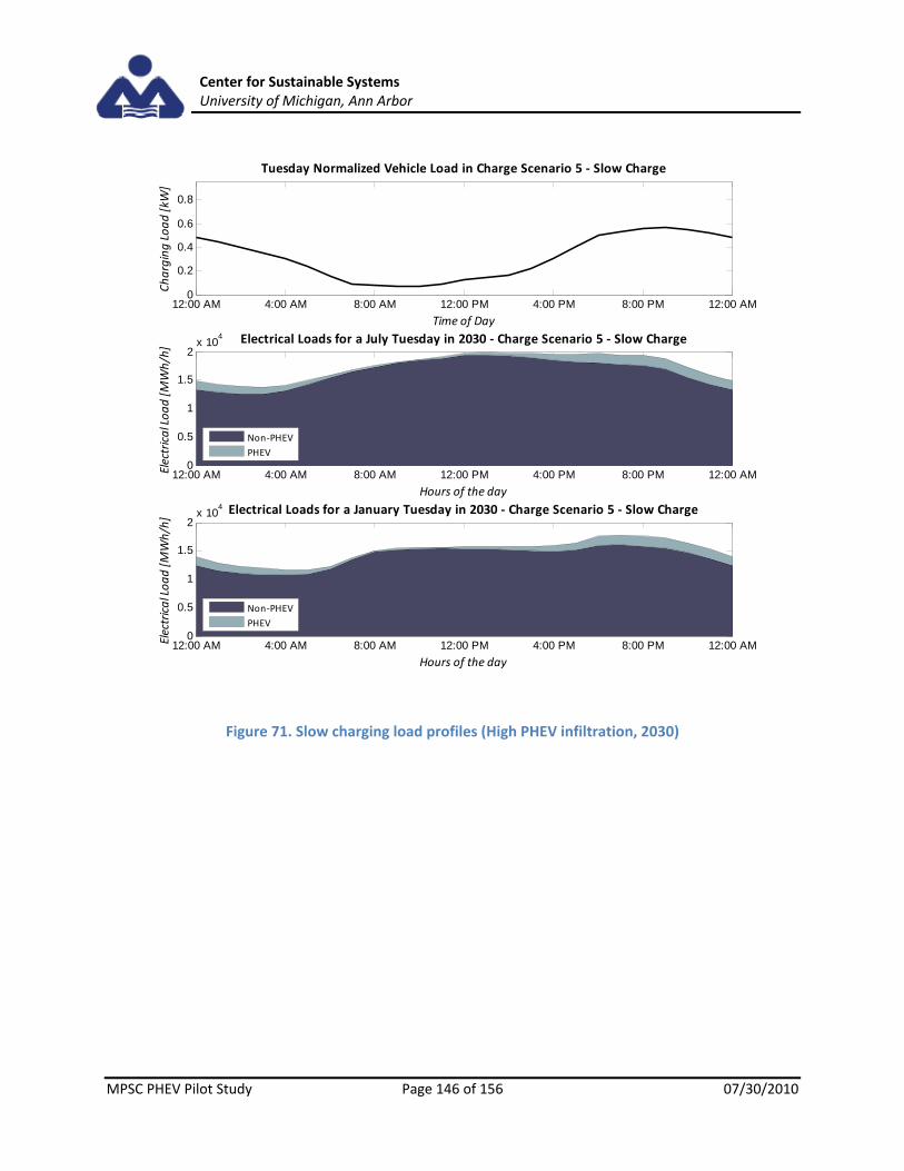
Center for Sustainable Systems University of Michigan, Ann Arbor
MPSC PHEV Pilot Study Page 146 of 156 07/30/2010
Figure 71. Slow charging load profiles (High PHEV infiltration, 2030)
12:00 AM 4:00 AM 8:00 AM 12:00 PM 4:00 PM 8:00 PM 12:00 AM0
0.2
0.4
0.6
0.8
Tuesday Normalized Vehicle Load in Charge Scenario 5 ‐ Slow Charge
Time of Day
Charging Load [kW
]
12:00 AM 4:00 AM 8:00 AM 12:00 PM 4:00 PM 8:00 PM 12:00 AM0
0.5
1
1.5
2x 10
4 Electrical Loads for a July Tuesday in 2030 ‐ Charge Scenario 5 ‐ Slow Charge
Electrical Load [MWh/h]
Hours of the day
Non‐PHEV
PHEV
12:00 AM 4:00 AM 8:00 AM 12:00 PM 4:00 PM 8:00 PM 12:00 AM0
0.5
1
1.5
2x 10
4 Electrical Loads for a January Tuesday in 2030 ‐ Charge Scenario 5 ‐ Slow Charge
Electrical Load [MWh/h]
Hours of the day
Non‐PHEV
PHEV

Center for Sustainable Systems University of Michigan, Ann Arbor
MPSC PHEV Pilot Study Page 147 of 156 07/30/2010
Figure 72. Fast charging load profiles (High PHEV infiltration, 2030)
12:00 AM 4:00 AM 8:00 AM 12:00 PM 4:00 PM 8:00 PM 12:00 AM0
1
2
3
Tuesday Normalized Vehicle Load in Charge Scenario 6 ‐ Fast Charge
Time of Day
Charging Load [kW
]
12:00 AM 4:00 AM 8:00 AM 12:00 PM 4:00 PM 8:00 PM 12:00 AM0
1
2
3x 10
4 Electrical Loads for a July Tuesday in 2030 ‐ Charge Scenario 6 ‐ Fast Charge
Electrical Load [MWh/h]
Hours of the day
Non‐PHEV
PHEV
12:00 AM 4:00 AM 8:00 AM 12:00 PM 4:00 PM 8:00 PM 12:00 AM0
0.5
1
1.5
2x 10
4 Electrical Loads for a January Tuesday in 2030 ‐ Charge Scenario 6 ‐ Fast Charge
Electrical Load [MWh/h]
Hours of the day
Non‐PHEV
PHEV

Center for Sustainable Systems University of Michigan, Ann Arbor
MPSC PHEV Pilot Study Page 148 of 156 07/30/2010
Figure 73. Fast, Home‐work charging load profiles (High PHEV infiltration, 2030)
12:00 AM 4:00 AM 8:00 AM 12:00 PM 4:00 PM 8:00 PM 12:00 AM0
1
2
3
Tuesday Normalized Vehicle Load in Charge Scenario 7 ‐ Fast Charge, Home and Work
Time of Day
Charging Load [kW
]
12:00 AM 4:00 AM 8:00 AM 12:00 PM 4:00 PM 8:00 PM 12:00 AM0
1
2
3x 10
4Electrical Loads for a July Tuesday in 2030 ‐ Charge Scenario 7 ‐ Fast Charge, Home and Work
Electrical Load [MWh/h]
Hours of the day
Non‐PHEV
PHEV
12:00 AM 4:00 AM 8:00 AM 12:00 PM 4:00 PM 8:00 PM 12:00 AM0
0.5
1
1.5
2x 10
4Electrical Loads for a January Tuesday in 2030 ‐ Charge Scenario 7 ‐ Fast Charge, Home and Work
Electrical Load [MWh/h]
Hours of the day
Non‐PHEV
PHEV
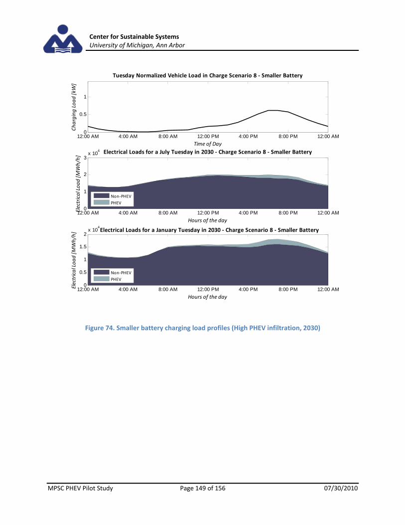
Center for Sustainable Systems University of Michigan, Ann Arbor
MPSC PHEV Pilot Study Page 149 of 156 07/30/2010
Figure 74. Smaller battery charging load profiles (High PHEV infiltration, 2030)
12:00 AM 4:00 AM 8:00 AM 12:00 PM 4:00 PM 8:00 PM 12:00 AM0
0.5
1
Tuesday Normalized Vehicle Load in Charge Scenario 8 ‐ Smaller Battery
Time of Day
Charging Load [kW
]
12:00 AM 4:00 AM 8:00 AM 12:00 PM 4:00 PM 8:00 PM 12:00 AM0
1
2
3x 10
4 Electrical Loads for a July Tuesday in 2030 ‐ Charge Scenario 8 ‐ Smaller Battery
Electrical Load [MWh/h]
Hours of the day
Non‐PHEV
PHEV
12:00 AM 4:00 AM 8:00 AM 12:00 PM 4:00 PM 8:00 PM 12:00 AM0
0.5
1
1.5
2x 10
4Electrical Loads for a January Tuesday in 2030 ‐ Charge Scenario 8 ‐ Smaller Battery
Electrical Load [MWh/h]
Hours of the day
Non‐PHEV
PHEV

Center for Sustainable Systems University of Michigan, Ann Arbor
MPSC PHEV Pilot Study Page 150 of 156 07/30/2010
Appendix I. Additional Greenhouse Gas Emissions Results
The following figures show the total system greenhouse gas emissions in 2030 for the electricity grid mix
simulations and for the charging simulations. Figure 75 shows results for the different electricity
generation mix simulations. Figure 76 shows results for the different charging simulations.
Figure 75. Total GHG for the year 2030 for all electricity grid mix simulations
Figure 76. Total GHG for the year 2030 for all charging simulations
EG1 EG2 EG3 EG40
2
4
6
8
10x 10
10
kg GHG, Electricity and Transportation sectors
Electricity Upstream
Electricity Generation
PHEV Gasoline Upstream
PHEV Gasoline Combustion
CV Gasoline Upstream
CV Gasoline Combustion
CH1 CH2 CH3 CH4 CH5 CH6 CH7 CH80
2
4
6
8
10x 10
10
kg GHG, Electricity and Transportation sectors
Electricity Upstream
Electricity Generation
PHEV Gasoline Upstream
PHEV Gasoline Combustion
CV Gasoline Upstream
CV Gasoline Combustion

Center for Sustainable Systems University of Michigan, Ann Arbor
MPSC PHEV Pilot Study Page 151 of 156 07/30/2010
Appendix J. Additional Criteria Pollutant Results
The data tables below show the criteria air pollutant emission rates pertinent to the results discussion in
this study’s report.
Table 54. Criteria air pollutant emission rates, 2030, EG1
EG1 Simulation CO Pb NOX PM2.5 PM10 VOC SOX
mil kg kg mil kg mil kg mil kg mil kg mil kg
FI4 Total Emissions 271 5,165 134 2.56 49.85 29.6 360
FI1 Total Emissions 348 4,963 141 3.39 49.79 34.9 341
Percentage Change ‐22% 4% ‐5% ‐25% 0.1% ‐15% 5%
FI4 CV&PHEV Emissions Average 247 378 32 2.56 8.6 20.9 34
FI4 CV&PHEV Emissions Marginal 248 203 24 2.56 7.1 21.4 29
FI1 CV Emissions 325 ‐ 32 3.39 7.1 26.8 10
Percentage Change Average ‐24% N/A 1% ‐25% 21% ‐22% 222%
Percentage Change Marginal ‐24% N/A ‐23% ‐25% 1% ‐20% 178%
Table 55. Criteria air pollutant emission rates, 2030, EG4
EG4 Simulation CO Pb NOX PM2.5 PM10 VOC SOX
mil kg kg mil kg mil kg mil kg mil kg mil kg
FI4 Total Emissions 264 2,252 80.4 2.56 26.56 28.6 256
FI1 Total Emissions 342 2,305 88.6 3.39 28.47 34.3 239
Percentage Change ‐23% ‐2% ‐9% ‐25% ‐7% ‐17% 7%
FI4 CV&PHEV Emissions Average 247 168 28.2 2.56 6.92 20.8 26
FI4 CV&PHEV Emissions Marginal 247 ‐53.16 23.7 2.56 5.17 21.1 28
FI1 CV Emissions 325 ‐ 31.9 3.39 7.08 26.8 10
Percentage Change Average ‐24% N/A ‐11% ‐25% ‐2% ‐22% 151%
Percentage Change Marginal ‐24% N/A ‐26% ‐25% ‐27% ‐21% 163%
Figure 77 through Figure 83 display the total system criteria pollutant emissions under the EG1
scenario for charging scenarios CH2 through CH8. The following remarks on the data represented in
these figures is based on the difference in results shown from the results under the baseline charging
scenario (CH1) discussed in detail in subsection 5.3. For each of the following figures, the emissions
which displayed a significant change in emissions levels from those of CH1 are noted. Further detail on
the cause of the observed trends is omitted. Specific explanations about the driving forces behind
changes of each emissions level can be referenced in the criteria air pollutants results discussion section

Center for Sustainable Systems University of Michigan, Ann Arbor
MPSC PHEV Pilot Study Page 152 of 156 07/30/2010
of the main report body (subsection 5.3).
Figure 77. Change in total system criteria air pollutants, 2030 (CH2, EG1, FI4)
In the CH2 scenario, the most significant changes are the increase in lead, decrease in NOX,
increase in PM10 and increase in SOX.
Figure 78. Change in total system criteria air pollutants, 2030 (CH3, EG1, FI4)
In CH3 scenario, the most significant changes are the decrease in NOX and decrease in PM10.
CO Pb NOx PM2.5 PM10 VOC SOx-25
-20
-15
-10
-5
0
5
10y ( )
Pe
rce
nt C
ha
ng
e fr
om
FI1
CO Pb NOx PM2.5 PM10 VOC SOx-30
-25
-20
-15
-10
-5
0
5
10y ( , , )
Pe
rce
nt C
ha
ng
e fr
om
FI1
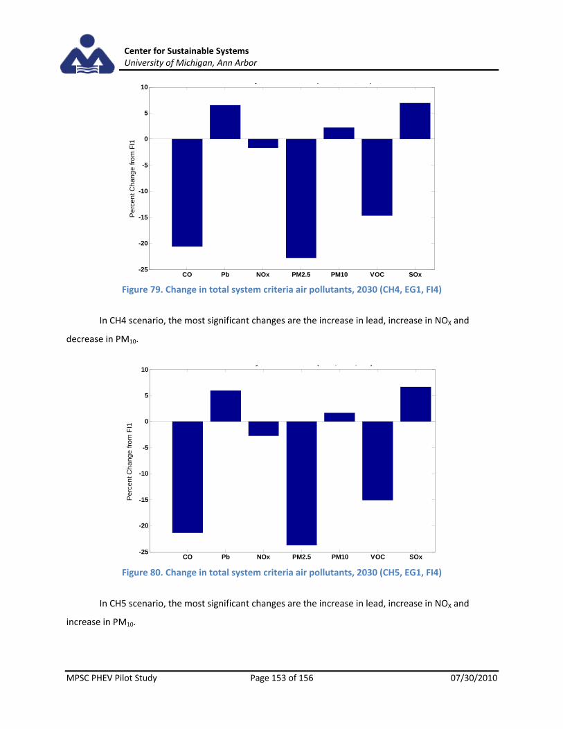
Center for Sustainable Systems University of Michigan, Ann Arbor
MPSC PHEV Pilot Study Page 153 of 156 07/30/2010
Figure 79. Change in total system criteria air pollutants, 2030 (CH4, EG1, FI4)
In CH4 scenario, the most significant changes are the increase in lead, increase in NOX and
decrease in PM10.
Figure 80. Change in total system criteria air pollutants, 2030 (CH5, EG1, FI4)
In CH5 scenario, the most significant changes are the increase in lead, increase in NOX and
increase in PM10.
CO Pb NOx PM2.5 PM10 VOC SOx-25
-20
-15
-10
-5
0
5
10y ( , , )
Pe
rce
nt C
ha
ng
e fr
om
FI1
CO Pb NOx PM2.5 PM10 VOC SOx-25
-20
-15
-10
-5
0
5
10y ( , , )
Pe
rce
nt C
ha
ng
e fr
om
FI1

Center for Sustainable Systems University of Michigan, Ann Arbor
MPSC PHEV Pilot Study Page 154 of 156 07/30/2010
Figure 81. Change in total system criteria air pollutants, 2030 (CH6, EG1, FI4)
In CH6 scenario, the most significant changes are the decrease in lead, decrease in NOX,
decrease in PM10, and decrease in SOX.
Figure 82. Change in total system criteria air pollutants, 2030 (CH7, EG1, FI4)
In CH7 scenario, the most significant changes are the decrease in lead, decrease in NOX and
decrease in PM10.
CO Pb NOx PM2.5 PM10 VOC SOx-30
-25
-20
-15
-10
-5
0
Pe
rce
nt C
ha
ng
e fr
om
FI1
CO Pb NOx PM2.5 PM10 VOC SOx-30
-25
-20
-15
-10
-5
0
5y ( )
Pe
rce
nt C
ha
ng
e fr
om
FI1
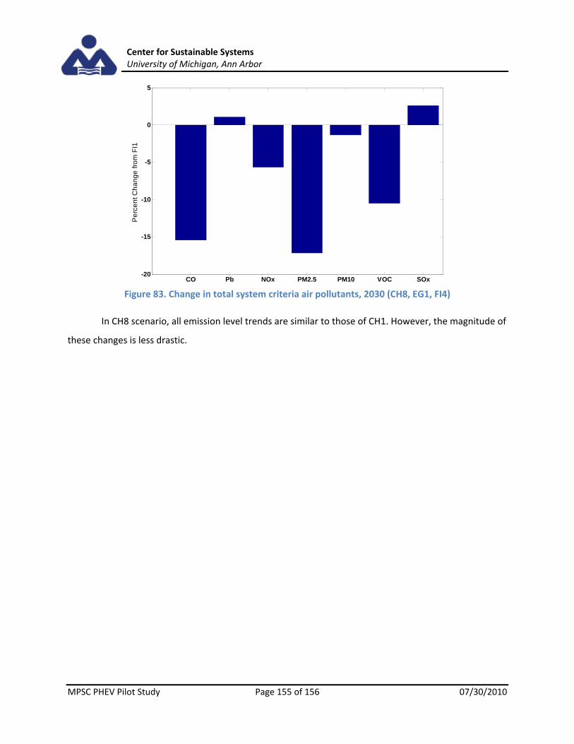
Center for Sustainable Systems University of Michigan, Ann Arbor
MPSC PHEV Pilot Study Page 155 of 156 07/30/2010
Figure 83. Change in total system criteria air pollutants, 2030 (CH8, EG1, FI4)
In CH8 scenario, all emission level trends are similar to those of CH1. However, the magnitude of
these changes is less drastic.
CO Pb NOx PM2.5 PM10 VOC SOx-20
-15
-10
-5
0
5y ( )
Pe
rce
nt C
ha
ng
e fr
om
FI1

Center for Sustainable Systems University of Michigan, Ann Arbor
MPSC PHEV Pilot Study Page 156 of 156 07/30/2010
References
1. Obama, B. and J. Biden. New Energy For America. 2008 [cited 2010 July 22]; Available from: http://www.barackobama.com/pdf/factsheet_energy_speech_080308.pdf.
2. Bandivadekar, A., et al., On the Road in 2035: Reducing Transportation’s Petroleum Consumption and GHG Emissions. MIT LFEE Report, 2008.
3. Kromer, M.A. and J.B. Heywood, A Comparative Assessment of Electric Propulsion Systems in the 2030 US Light‐Duty Vehicle Fleet. SAE Technical Papers, 2008.
4. Stephan, C.H. and J. Sullivan, Environmental and Energy Implications of Plug‐In Hybrid‐Electric Vehicles. Environmental Science and Technology, 2008.
5. Grimes‐Casey, H.G., G.A. Keoleian, and B. Willcox, Carbon Emission Targets for Driving Sustainable Mobility with US Light‐Duty Vehicles. Environmental Science and Technology, 2009. 43(3): p. 585‐590.
6. Electric Power Research Institute, Environmental Assessment of Plug‐In Hybrid Electric Vehicles. 2007.
7. Hajian, M., H. Zareipour, and W. Rosehart, Environmental Benefits of Plug‐in Hybrid Electric Vehicles: the Case of Alberta. IEEE, 2009.
8. Minnesota Pollution Control Agency, Minnesota Plug‐in Hybrid Electric Vehicle Task Force: Report to the Minnesota Legislature. 2007.
9. Samaras, C. and K. Meisterling, Life Cycle Assessment of Greenhouse Gas Emissions from Plug‐in Hybrid Vehicles: Implications for Policy. Environmental Science and Technology, 2008. 42(9): p. 3170‐3176.
10. McCarthy, R. and C. Yang, Determining marginal electricity for near‐term plug‐in and fuel cell vehicle demands in California: Impacts on vehicle greenhouse gas emissions. Journal of Power Sources, 2010(195): p. 2099 ‐ 2109.
11. Kintner‐Meyer, M., K. Schneider, and R. Pratt, Impacts Assessment of Plug‐in Hybrid Vehicles on Electric Utilities and Regional U.S Power Grids Part 1: Technical Analysis. Pacific Northwest National Laboratory Report, 2007.
12. Thompson, T., M. Webber, and D.T. Allen, Air quality impacts of using overnight electricity generation to charge plug‐in hybrid electric vehicles for daytime use Environmental Research Letters 2009. 4(1).
13. Sivaraman, D. and G.A. Keoleian, Photovoltaic (PV) electricity: Comparative analyses of CO2 abatement at different fuel mix scales in the US. Energy Policy. In Press, Corrected Proof.
14. Federal Highway Administration, National Household Travel Survey (NHTS) vers. 1.0. 2009. 15. DOE ‐ Energy Efficiency and Renewable Energy, E., Fueleconomy.gov ‐ official government source
of fuel economy information. 16. W. Short, P.D., A Preliminary Assessment of Plug‐In Hybrid Electric Vehicles on Wind Energy
Markets. 2006, National Renewable Energy Laboratory. 17. Blanco, S. GM shows off 120V and 240V chargers for 2011 Chevy Volt. 2009; Available from:
http://green.autoblog.com/2009/08/11/gm‐shows‐off‐120v‐and‐240v‐chargers‐for‐2011‐chevy‐volt/.
18. Sioshansi, R. and P. Denholm, Emissions Impacts and Benefits of Plug‐In Hybrid Electric Vehicles and Vehicle‐to‐Grid Services. Environmental Science and Technology, 2009. 43(4): p. 1199‐1204.
19. Bashash, S., et al., Plug‐in Hybrid Electric Vehicle Charge Pattern Optimization for Energy Cost and Battery Longevity. Journal of Power Sources, 2010. In Press, Accepted Manuscript.
20. Energy Information Administration. 2009 Annual Energy Outlook. 2009 [cited 2009 November

Center for Sustainable Systems University of Michigan, Ann Arbor
MPSC PHEV Pilot Study Page 157 of 156 07/30/2010
9]; Available from: http://www.eia.doe.gov/oiaf/aeo/index.html. 21. U.S. Census Bureau, Census 2000 Data for the State of Michigan. 2000. 22. Michigan Department of State, TR/9050 ‐ Total Registered Vehicles. 2009. 23. Department of Transportation Federal Highway Administration, Highway Statistics Series. 2008. 24. National Renewable Energy Laboratory, U.S. Life‐Cycle Inventory Database. 25. Environmental Protection Agency, eGRID. 2007. 26. Michigan Public Service Commission, 21st Century Energy Plan, C.N. Forum, Editor. 2007. 27. State of Michigan, Clean, Renewable and Efficient Energy Act, MPSC, Editor. 2008. 28. Office of the Governor. Granholm: Energy Plan, Investments in Alternative Energy Will Create
Jobs, Grow Economy. 2007 [cited 2009 May 29]; Available from: http://www.michigan.gov/gov/0,1607,7‐168‐23442_21974‐167376‐‐,00.html.
29. DTE Energy. Renewable Energy Plan Overview. 2009 March 6, 2009 [cited 2009 Nov. 19]; Available from: http://www.dteenergy.com/dteEnergyCompany/investors/pdfs/summaryRenewablesEO.pdf.
30. Consumers Energy, Balanced Energy Initiative: Electric Generation Alternatives Analysis. 2009. 31. National Renewable Energy Laboratory. Wind Integration Datasets ‐ MISO. 2008 [cited 2009
Nov. 20]; Available from: http://www.nrel.gov/wind/integrationdatasets/eastern/data.html. 32. WorldEnergy.org, EPRI Generation Options under a Carbon Constrained Future – Reference Data;
Representative Cost and Performance of Power Generation Technologies. 2007. 33. Detroit Edison, The Detroit Edison Company Summer 2009 Resource Adequacy Plan. 2009. 34. North American Electricity Reliability Corporation, 2004‐2008 Generating Unit Statistical
Brochure. 2009, North American Electric Reliability Corporation: Princeton. 35. COO, B.H.M. MAPP Generation Reserve Sharing Pool 2006; Available from:
http://www.misostates.org/R3%20‐%20Bill%20Head,%20MAPP.pdf. 36. Energy Information Administration, Form 906/920/923 Electricity Database Files. 2005. 37. Federal Energy Regulatory Commission, Form 714: Annual Electric Control and Planning Area
Report. 2009. 38. Intergovenmental Panel on Climate Change, Fourth Assessment Report: Climate Change. 2007. 39. Energy Information Administration. 2010 Annual Energy Outlook. 2010 [cited 2010 February 5];
Available from: http://www.eia.doe.gov/oiaf/aeo/index.html. 40. Environmental Protection Agency, EPA Analysis of the American Clean Energy and Security Act of
2009, H.R. 2454 in the 111th Congress, E.P. Agency, Editor. 2009. 41. NREL: U.S. Life‐Cycle Inventory Database. 2008. 42. Argonne GREET Model, in Transportation Technology R&D Center. 2009. 43. Lemoine, D., D. Kammen, and A. Farrell, An innovation and policy agenda for commercially
competitive plug‐in hybrid elecric vehicles. Environmental Research Letters, 2008. 44. Vyas, A., D. Santini, and L. Johnson, Plug‐In Hybrid Electric Vehicles’ Potential for Petroleum Use
Reduction: Issues Involved in Developing Reliable Estimates, in 88th Annual Meeting of the Transportation Research Board. 2009.
45. U.S. Census Bureau, American Housing Survey for the United States: 2005. 2006, U.S. Governement Printing Office.
46. Federal Highway Administration, National Household Transportation Survey (ver. 2001). 2005. 47. PA 295 ‐ Clean, Renewable and Efficient Energy Act, in PA 295. 2008. 48. U.S. Department of Energy. Alternative Fuels & Advanced Vehicles Data Center, HEV sales by
model,. 2009; Available from: http://www.afdc.energy.gov/afdc/data/vehicles.html. 49. Shiau, C.‐S.N., et al., Impact of Battery Weight and Charging Patterns on the Economic and

Center for Sustainable Systems University of Michigan, Ann Arbor
MPSC PHEV Pilot Study Page 158 of 156 07/30/2010
Environmental Benefits of Plug‐in Hybrid Vehicles, in 88th Annual Meeting of the Transportation Research Board. 2009.
50. Samaras, C., et al., Policies to Promote Plug‐in Hybrid Electric Vehicles for Greenhouse Gas Emissions Reductions and Oil Displacement, in 88th Annual Meeting of the Transportation Research Board. 2009.
51. California Public Utilities Commission. California Renewable Portfolio Standards. 2006; Available from: http://www.cpuc.ca.gov/PUC/energy/Renewables/index.htm.
52. U.S. Census Bureau. Michigan QuickFacts from the US Census Bureau. 2010 [cited 2010 May 11]; Available from: http://quickfacts.census.gov/qfd/states/26000.html.
53. Michigan Live News ‐ David Eggert. New coal‐fired power plants opposed in Michigan. 2008; Available from: http://www.mlive.com/environment/index.ssf/2008/04/new_coalfired_power_plants_opp.html.
54. John Axsen, K.K., Ryan McCarthy, Christopher Yang,, Plug‐in hybrid vehicle GHG impacts in California: Integrating consumer‐informed recharge profiles with an electricity‐dispatch model 2010.
55. U.S. Environmental Protection Agency. Six Common Criteria Air Pollutants. Available from: http://www.epa.gov/air/urbanair/.
56. U.S. Environmental Protection Agency, Clean Air Act, in 42. 1990. 57. Michigan Department of Natural Resources and Environment. MDEQ ‐ Michigan Air Emissions
Reporting System (MAERS). 2009; Available from: http://www.michigan.gov/deq/0,1607,7‐135‐3310_4103_4193‐16768‐‐,00.html.
58. Michigan Public Service Commission. Electric Utility Sales Data. 2009 [cited 2009 June 29]; Available from: http://www.michigan.gov/mpsc/0,1607,7‐159‐16377_52818‐‐‐,00.html.
59. Energy Information Administration. Annual Energy Review 2007. 2007 [cited 2009 August 19]; Available from: http://www.eia.doe.gov/emeu/aer/pdf/pages/secnote2.pdf.
60. Energy Information Administration. Table A4. Approximate Heat Content of Natural Gas, 1949‐2008. 2009 [cited 2009 August 19]; Available from: http://www.eia.doe.gov/emeu/aer/txt/ptb1304.html.
61. Adornato, B.P., R.; Filipi, Z.; Baraket, Z.; Gordon, T.;, Characterizing naturalistic driving patterns for Plug‐in Hybrid Electric Vehicle analysis. Vehicle Power and Propulsion Conference, 2009. VPPC '09. IEEE 2009: p. 655‐660.
62. Kwon, J., et al., Impact of Drive Cycles on PHEV Component Requirements. SAE Technical Papers, 2008.
63. Kammen, D.A.S.L., D.; Hummel, H., Cost‐Effectiveness of Greenhouse Gas Emission Reductions from Plug‐in Hybrid Electric Vehicles. Goldman School of Public Policy Working Paper No. GSPP08‐014, 2008.