Energies 2013, 6, 3134-3148; doi:10.3390/en6073134

energies ISSN 1996-1073

www.mdpi.com/journal/energies

Article

The Analysis of the Aerodynamic Character and Structural Response of Large-Scale Wind Turbine Blades

Xin Cai 1,2, Pan Pan 1,*, Jie Zhu 1 and Rongrong Gu 1

1 College of Mechanics and Materials, Hohai University, Nanjing 210098, China;

E-Mails: xcai@hhu.edu.cn (X.C.); zhukejie2222@163.com (J.Z.); gurr99@126.com (R.G.) 2

College of Water Conservancy and Hydropower Engineering, Hohai University,

Nanjing 210098, China

* Author to whom correspondence should be addressed; E-Mail: panpan.159@163.com;

Tel.: +86-159-5057-9343; Fax: +86-519-8510-3280.

Received: 22 April 2013; in revised form: 20 June 2013 / Accepted: 20 June 2013 /

Published: 27 June 2013

Abstract: A process of detailed CFD and structural numerical simulations of the 1.5 MW

horizontal axis wind turbine (HAWT) blade is present. The main goal is to help advance

the use of computer-aided simulation methods in the field of design and development of

HAWT-blades. After an in-depth study of the aerodynamic configuration and materials of

the blade, 3-D mapping software is utilized to reconstruct the high fidelity geometry, and

then the geometry is imported into CFD and structure finite element analysis (FEA)

software for completely simulation calculation. This research process shows that the CFD

results compare well with the professional wind turbine design and certification software,

GH-Bladed. Also, the modal analysis with finite element method (FEM) predicts well

compared with experiment tests on a stationary blade. For extreme wind loads case that by

considering a 50-year extreme gust simulated in CFD are unidirectional coupled to the

FE-model, the results indicate that the maximum deflection of the blade tip is less than the

distance between the blade tip (the point of maximum deflection) and the tower, the material

of the blade provides enough resistance to the peak stresses the occur at the conjunction of

shear webs and center spar cap. Buckling analysis is also included in the study.

Keywords: rotational effect; fluid structure interaction; eigenbuckling; Mieses stress

OPEN ACCESS

Energies 2013, 6 3135

1. Introduction

To capture higher wind speeds, wind turbines have increased in height and size and this reduces the

number of individual turbine units possible on a wind farm and in turn the cost of operation of the

farm. For example, the first 5 MW offshore wind turbine unit with a rotor diameter of 115 m, and a

hub height reaching more than 100 m has been recently installed in the Fujian Province of China.

To design and develop more efficient and reliable wind turbines, the way to accurately predict

aerodynamic characteristics and structure response is of critical significance. There are various

classical aerodynamic models available in the literature: The blade element momentum (BEM) method

could be a design as well as a verification tool which splits the blade into small elements, airfoil data

of each element is provided for lift and drag coefficients as a function of angle of attack, so

performance of the turbine can be calculated by summing the contribution of all the elements [1]; to

obtain more aerodynamic characteristics of wind turbines, studies of the wake configuration have been

likewise been conducted. The prescribed-vortex wake [2], free-vortex wake method [3] as well as

lifting panel method [4] show good application prospects. In recent years, advances in computer

technology that enabled computational fluid dynamics (CFD) techniques to deal with more

aerodynamic issues, like boundary layer transition, dynamic stall, inflow turbulence, rotational effects,

and so on. On the other hand, CFD analysis of wind turbines can be performed at a lesser cost than that

required to set up a wind tunnel and perform full scale experiments. There has been a growing use of

CFD codes over the last decade for turbine blade performance analysis, among them the ANSYS CFX

software has a good reputation for its good performance on turbo-machinery simulation, as well as

aeroelasticity analysis [5,6].

To investigate the global behaviors in terms of, for example, eigenfrequencies, tip deflections,

buckling, and global stress/strain levels of wind turbine blades at certain wind speeds, finite element

methods (FEM) have gained wider acceptance as they have become more capable in their predictive

capability. In [7], Jensen used FE-code MSC-Marc to simulate the Brazier effect of the load-carrying

box girder of a 34 m composite blade. Hermann [8] and Raiauurai [9] applied ANSYS software to

simulate the buckling and free vibration behavior of wind turbine blades, respectively.

Grujicic [10,11] used ABAQUS/Standard to calculate the equivalent strain and Von Mises distribution

over the large-scale HAWT-blade caused by a 70 m/s gust.

Rotor blade shells are made of monolithic composite laminates in the root and main spar areas, and

the other parts include webs constructed with sandwich composites. However, the laminates are

assembled of various fibrous layers in the entire blade and vary in thickness along the longitudinal as

well as the transverse direction due to the “ply drop” [12]. In order to predict the global behaviors

accurately, intensive effort must be devoted to investigate the material properties, the start and end

position, the amount and sequence of the various layers of the assigned laminates.

The main objective of this paper is to adopt commercial software, like CFX and ANSYS, to

simulate a wind turbine blade which has already been installed and put into operation under certain

conditions, and compare these results to experimental tests and some international certification

standards. It is hoped that a set of computer-aided approaches could be put forward in the wind turbine

blades design/development area so that many critical decisions and modifications can be made to

improve the quality of large-scale HAWT-blades.

Energies 2013, 6 3136

The paper is organized as follows: Section 2 presents detailed specifications of the 1.5 MW

HAWT-blade. Section 3 presents the CFD simulation and aerodynamics characteristics of this blade.

Section 4 presents the accurate FE-model constructing and dynamic characteristics of this blade, and

then its static behaviors under limit loads obtained in Section 3 are calculated. The simulation results

provide several suggestions for further modification of large-scale blades. Section 5 summaries the key

conclusions resulting from the present work.

2. Specifications of 1.5 MW Wind Turbine Blade

The rotor blade investigated in this paper is designed for a 3-blade upwind wind turbine, which is

nominally 37.5 m long and controlled by the pitch-regulated variable speed method. The

thickness-to-chord ratio (t/c) of the airfoils chosen for the blade varies from 40% in the blade shoulder

(r/R = 0.215) to 18% in the blade tip. The difference between the maximum and minimum twist angle

is 8.78°. The diameter of the cylindrical blade root is 1.8 m, and the length of the cord in the blade

shoulder is 3.08 m. The specific configurations of the blade are summarized in Table 1.

Table 1. Specifications of the 1.5 MW wind turbine blade.

Parameters Value

Rated wind speed (m/s) 11.5 Rated rotor speed (rpm) 19.0 Cut in wind speed (m/s) 3.5 Cut out wind speed (m/s) 25.0 Extreme wind speed (m/s) 59.0

Rotor overhang (m) 4.2

3. Aerodynamic Analysis

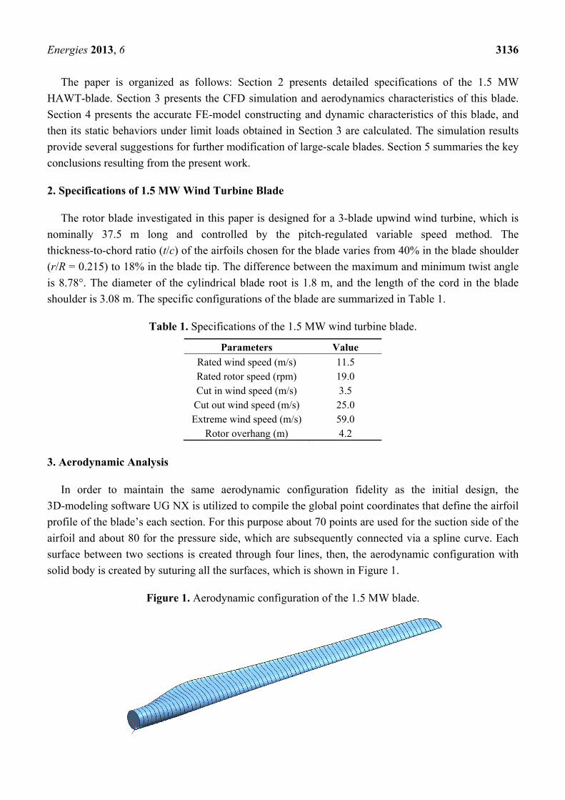
In order to maintain the same aerodynamic configuration fidelity as the initial design, the

3D-modeling software UG NX is utilized to compile the global point coordinates that define the airfoil

profile of the blade’s each section. For this purpose about 70 points are used for the suction side of the

airfoil and about 80 for the pressure side, which are subsequently connected via a spline curve. Each

surface between two sections is created through four lines, then, the aerodynamic configuration with

solid body is created by suturing all the surfaces, which is shown in Figure 1.

Figure 1. Aerodynamic configuration of the 1.5 MW blade.

Energies 2013, 6 3137

3.1. Simulation Method

In the present work, only one of the three blades is explicitly modeled in the computations. The

remaining blades are accounted for using periodic boundary conditions, exploiting the 120° symmetry

of the three-bladed rotor, therefore, a 1/3 cylindrical numerical wind tunnel is constructed in the UG

NX. The numerical tunnel consists of two domains, namely the rotational domain which contains the

blade, and the stationary domain. The rotational domain is defined by the reference length of the rotor

radius of 39 m. A spatial resolution of 102 m to the calculation domain inlet, 340 m to the downstream

region, and 140 m to the radial direction of the wind tunnel is applied.

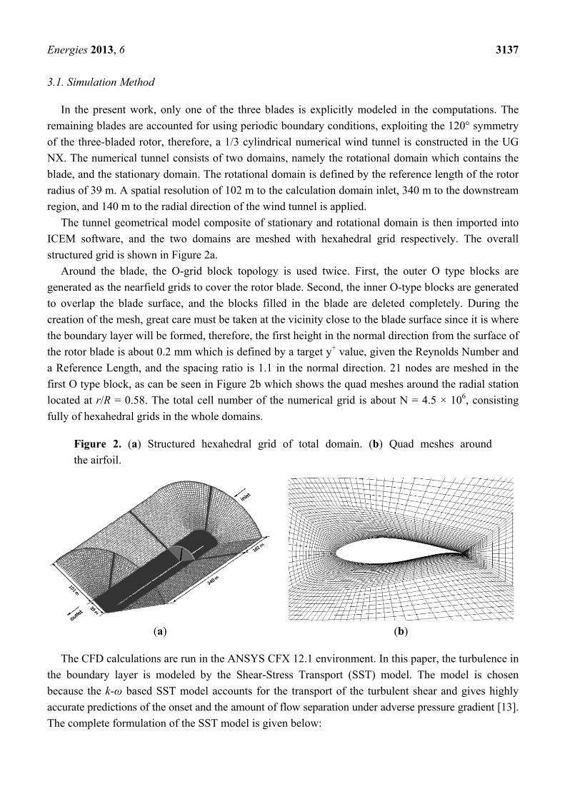
The tunnel geometrical model composite of stationary and rotational domain is then imported into

ICEM software, and the two domains are meshed with hexahedral grid respectively. The overall

structured grid is shown in Figure 2a.

Around the blade, the O-grid block topology is used twice. First, the outer O type blocks are

generated as the nearfield grids to cover the rotor blade. Second, the inner O-type blocks are generated

to overlap the blade surface, and the blocks filled in the blade are deleted completely. During the

creation of the mesh, great care must be taken at the vicinity close to the blade surface since it is where

the boundary layer will be formed, therefore, the first height in the normal direction from the surface of

the rotor blade is about 0.2 mm which is defined by a target y+ value, given the Reynolds Number and

a Reference Length, and the spacing ratio is 1.1 in the normal direction. 21 nodes are meshed in the

first O type block, as can be seen in Figure 2b which shows the quad meshes around the radial station

located at r/R = 0.58. The total cell number of the numerical grid is about N = 4.5 × 106, consisting

fully of hexahedral grids in the whole domains.

Figure 2. (a) Structured hexahedral grid of total domain. (b) Quad meshes around

the airfoil.

(a) (b)

The CFD calculations are run in the ANSYS CFX 12.1 environment. In this paper, the turbulence in

the boundary layer is modeled by the Shear-Stress Transport (SST) model. The model is chosen

because the k-ω based SST model accounts for the transport of the turbulent shear and gives highly

accurate predictions of the onset and the amount of flow separation under adverse pressure gradient [13].

The complete formulation of the SST model is given below:

Energies 2013, 6 3138

2 21 2

( )( )( )

( )( ) 1( ) 2(1 )

ik k t

i i i

it

i i i i i

U kk kP k

t x x x

U kS F

t x x x x xω ω

ρρ β ρ ω μ σ μ

ρ ωρω ω ωαρ βρω μ σ μ ρσω

∗ ∂∂ ∂ ∂+ = − + + ∂ ∂ ∂ ∂

∂∂ ∂ ∂ ∂ ∂ + = − + + + − ∂ ∂ ∂ ∂ ∂ ∂

(1)

where the blending function F1 is defined by:

4

21 2 2

4500tanh min max , ,

k

kk vF

y y CD yω

ω

ρσβ ω ω∗

=

(2)

where 102

1max 2 ,10k

i i

kCD

x xω ωωρσ

ω− ∂ ∂= ∂ ∂

; y is the distance to the nearest wall; v is the

kinematic viscosity.

F1 is equal to zero away from the surface (k-ε model), and switches over to one inside the boundary

layer (k-ω model).

The proper transport behavior can be obtained by a limiter to the formulation of the eddy-viscosity,

which is defined as follows:

1

1 2max( , )t

a kv

a SFω= (3)

where S is the invariant measure of the strain rate and F2 is a second blending function defined by:

2

2 2

2 500tanh max ,

k vF

y yβ ω ω∗

= (4)

A production limiter is used in the SST model to prevent the build-up of turbulence in

stagnation regions:

min( ,10 )ji ik t k k

j j i

UU UP P P k

x x xμ β ρ ω∗ ∂∂ ∂= + → = ∂ ∂ ∂

(5)

All constants are computed by a blend from the corresponding constants of the k-ε and the k-ω model via 1 2 (1 )F Fα α α= + − . The constants for this model are: 0.09β ∗ = ; 1 5 / 9α = ; 1 3 / 40β = ;

1 0.85kσ = ; 1 0.5ωσ = ; 2 0.44α = ; 2 0.0828β = ; 2 1kσ = ; 2 0.856ωσ = .

For the boundary conditions, a normal speed condition with a lower turbulent intensity of 14%

which is defined in IEC 61400-1 standard [14] is applied at the inlet boundary, and an average static

pressure condition is applied at the outlet condition. No-slip condition is selected for the blade, nacelle

and outer domain surfaces. The periodic conditions are applied at the 120° cyclic boundaries.

For convergence control, because the meshes are refined nearby the blade surface, convergence

issues will arise since smaller flow features such as shedding phenomena will be resolved effectively,

which coarser meshes cannot capture. The value of the root mean square (RMS) normalized residual

over the whole domain is chosen to be below 10−4, and the maximum amount of iterations is set large

enough to monitor the blade torque until stabilization.

Before the CFD results are drawn, the grid-independent analysis is conducted. According to

Cimbala’s paper [15], the number of nodes of every block’s edges is increased by 20%, while the node

Energies 2013, 6 3139

number in the spanwise direction of the blade remains unchanged. After being simulated with the

above methods under rated conditions in steady state, the monitored torque doesn’t change appreciably

compared with initial mesh (error is within 2%), so the original grid is adequate.

3.2. CFD Results and Discussion

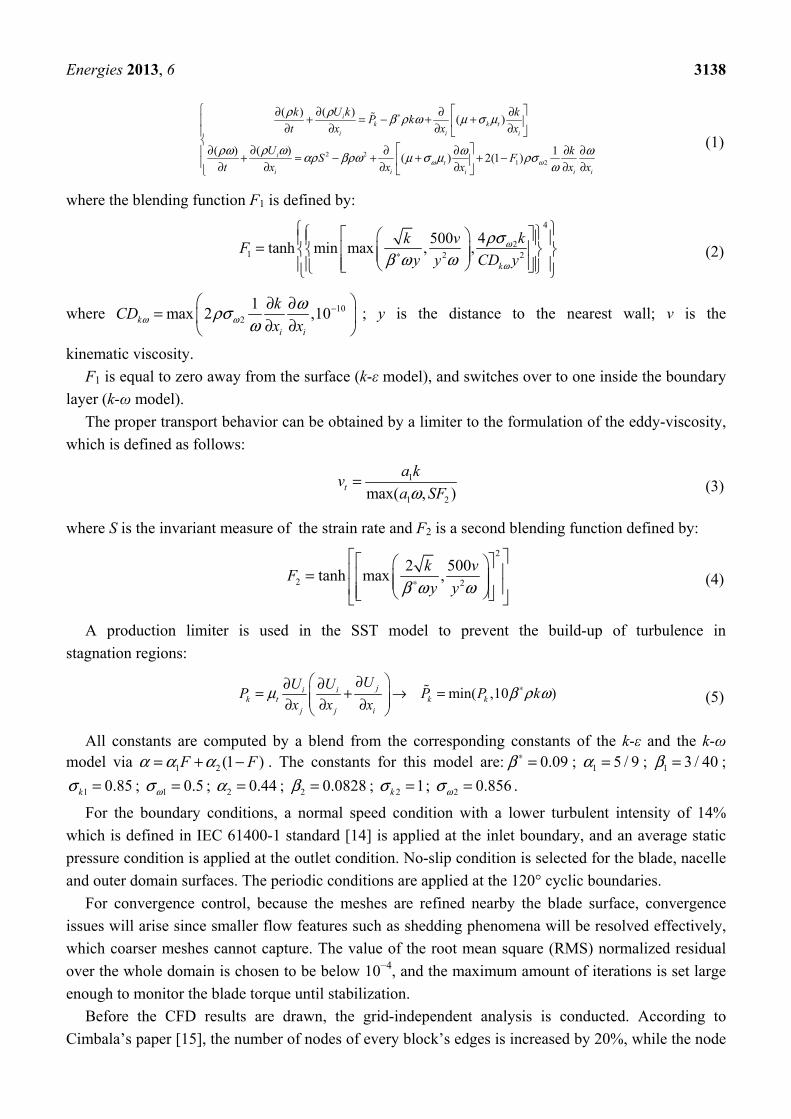
In this paper, six different inflow velocities, V∞ = 5, 6.5, 8, 9.5, 10.5, 11.5, 25 m/s are chosen for

rotor blade simulation in steady state, meanwhile, the pitch and torque controls are not considered. The

contour variations of fluid tangential forces which produce torque on the suction surface of the rotor

blade at three wind speeds (5, 11.5, 25 m/s) are shown in Figure 3. It is observed that the tangential

forces mainly concentrate at the outboard stations between r/R = 0.5~0.8 at lower wind speed, so the

rotor blade is not at its best to produce the maximum power coefficient. At the rated wind speed, the

tangential forces contour which appears towards the leading edge and can be observed almost from

blade tip to root illustrate that the rotor blade has good aerodynamic performance when pitched at 0°.

At 25 m/s, the blade is in deep stall, the calculated tangential force magnitude is in large scale as well

as the axial thrust. Therefore, the active control system should execute collective pitching or individual

pitching operation to reduce the angle of attack and hence the lift coefficient.

Figure 3. Fluid tangential forces contour on the suction side.

The power extraction from air and coefficient are defined in Equations (6) and (7):

2 / 60Power B T n π= ⋅ ⋅ ⋅ (6)

30.5P

PowerC

V Aρ ∞

=⋅ ⋅ ⋅ (7)

where B is the total number of blades; T is the torque of single blade; n is the rotor speed of wind

turbine; ρ is the air density; A is the rotor swept area; and V∞ is the flow velocity.

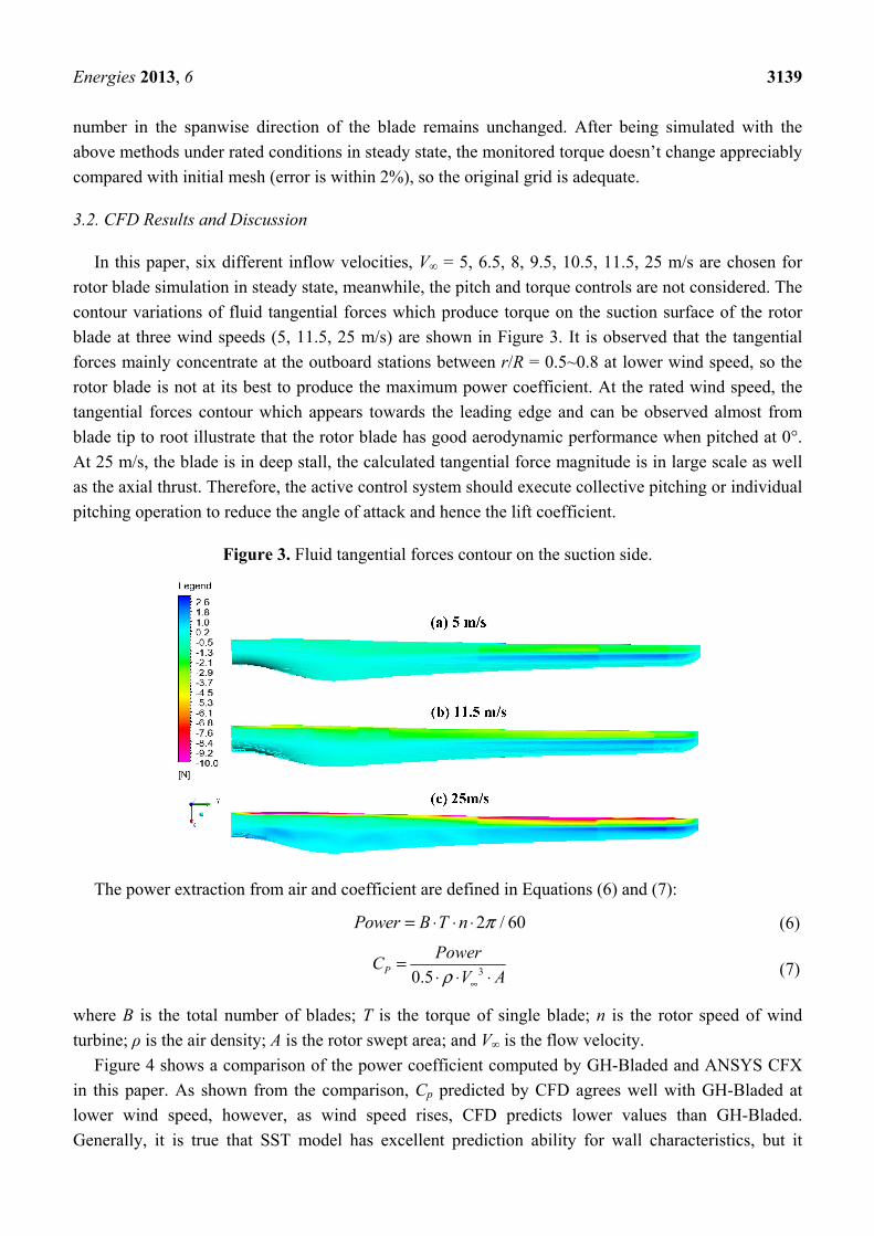
Figure 4 shows a comparison of the power coefficient computed by GH-Bladed and ANSYS CFX

in this paper. As shown from the comparison, Cp predicted by CFD agrees well with GH-Bladed at

lower wind speed, however, as wind speed rises, CFD predicts lower values than GH-Bladed.

Generally, it is true that SST model has excellent prediction ability for wall characteristics, but it

Energies 2013, 6 3140

usually underestimates the rotor torque in the stalled regime which would become evident as wind

speed rises.

Figure 4. Power coefficient comparison between CFX and GH-Bladed.

4 5 6 7 8 9 10 11 120.0

0.1

0.2

0.3

0.4

0.5Pow

er

Coe

ffic

ient

Wind Velocity(m/s)

ANSYS CFX

GH-Bladed

3.3. Rotational Effects

For the purpose of applying the BEM method, the stations of the blade are extracted at the interval

of 1 m. Each station is computed with 2-D CFD and determined the values of lift coefficient Cl and

drag coefficient Cd as function of attack angle. The power calculated by BEM is 1.762 MW, and the

axial thrust value is 306.60 kN, both are larger than CFD code (the values computed by CFD are

1.513 MW and 280.38 kN). In Figure 5, the radial stations located at r/R = 0.3, 0.6, 0.85 are chosen for

pressure comparison evaluated with 3-D and 2-D CFD in the rated condition, the airfoil profile form of

the three radial stations can be clearly seen in Figure 6. In the 2-D case, the aerodynamic load of each

radial station is computed with twist angle settled the same as its position in blade in the global

coordinates. By picking up the axial induction factor a and angular induction factor a' of each station

with BEM method, the equivalent speed input in 2-D simulation is defined in Equation (8):

2 2(1 ) ( (1 ))rrel

rV V a a

V∞∞

Ω ′= − + + (8)

where r is the radial station radius; Ωr is the angular velocity.

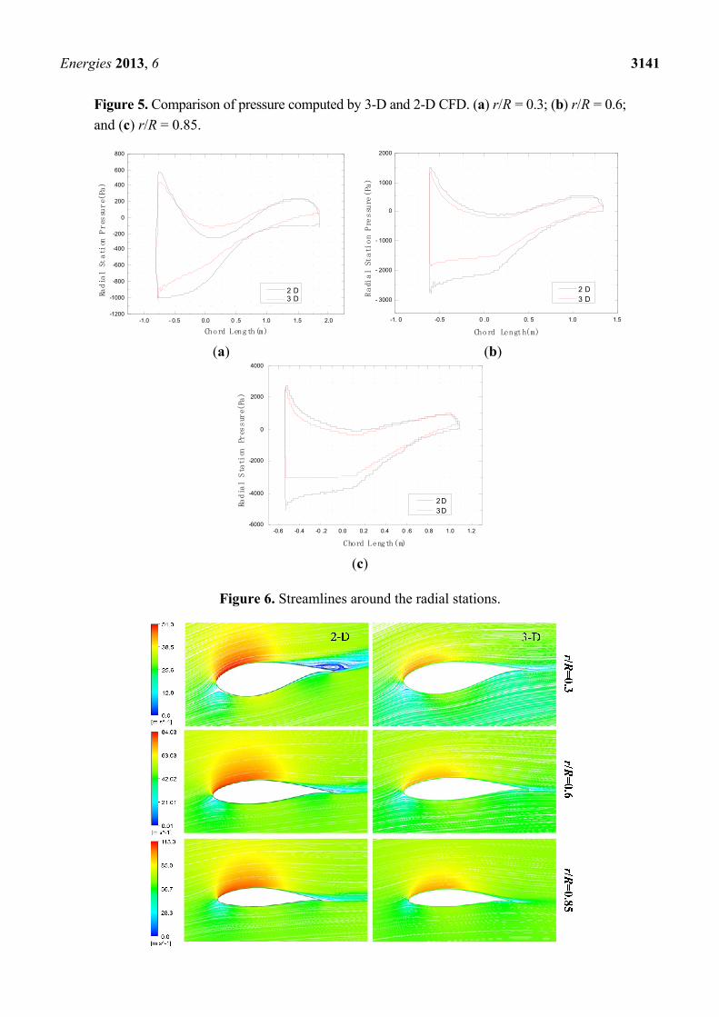
It can be seen that the distance between suction and pressure side, i.e., the area of the graph, looks

considerably larger in the 2-D case in the figure. Thus, a higher thrust is obtained when the BEM

method applied at the design point. At r/R = 0.3, the 2-D curve falls abruptly, whereas the 3-D trend is

smoother after the peak pressure on suction side. The pressure gradient of the flow has a significant

effect on the boundary layer, as illustrated in Figure 6, where the in-plane streamlines around the

rotating radial station and the corresponding pure 2-D stations are plotted. It is visible that the flow in

the boundary layer stops and reverses direction due to the rapid change pressure gradient in the 2-D case.

The separating flows from the station place it in stall condition, however, the main effects of rotation are

to stabilize vortex shedding and limit the growth of the separation layer, as seen in the 3-D case.

Energies 2013, 6 3141

Figure 5. Comparison of pressure computed by 3-D and 2-D CFD. (a) r/R = 0.3; (b) r/R = 0.6;

and (c) r/R = 0.85.

-1.0 - 0.5 0.0 0 .5 1.0 1.5 2.0-1200

-1000

-800

-600

-400

-200

0

200

400

600

800

Radia

l Stati

on P

res

sure(

Pa)

Chord Length(m)

2 D 3 D

-1. 0 -0.5 0 .0 0. 5 1.0 1.5

- 3000

- 2000

- 1000

0

1000

2000

Radial St

ati

on

Pre

ssure

(Pa

)

Chord Length(m)

2 D 3 D

(a) (b)

-0.6 -0.4 -0 .2 0.0 0.2 0.4 0 .6 0.8 1.0 1.2-6000

-4000

-2000

0

2000

4000

Radia

l Sta

tion

Pr

essure(

Pa)

Chord Length(m)

2 D 3 D

(c)

Figure 6. Streamlines around the radial stations.

Energies 2013, 6 3142

The present wind turbine design approach is typically based on BEM theory. Although the outboard

aerodynamic character which is plotted by limiting streamlines on the blade surface in Carcangiu’s

Ph.D. thesis [16] presents a 2D-alike behavior, the Coriolis and centrifugal forces obviously influence

the aerodynamic behavior in the inboard sections. Furthermore, the accurate prediction of rotor blade

loads in rotational state is of great importance for sizing the generator and other mechanical components.

4. Structural Analysis

4.1. Finite Element Modeling of the Blade

The blade geometry is modeled in UG NX as mentioned previously. The finite element model

(FEM) is developed in ANSYS software, and there exists a connection functionality which can provide

a convenient means to import blade geometry into ANSYS. Before meshing, the blade geometry is

divided into a large number of areas in order to define the structural characteristics, including spar

caps, shear webs, ply drops, etc. Every time there is a ply drop whatever in the spanwise or chordwise

direction, there must be a line to coincide with it because a new laminate definition is required. The

materials properties are collected in Table 2 as below.

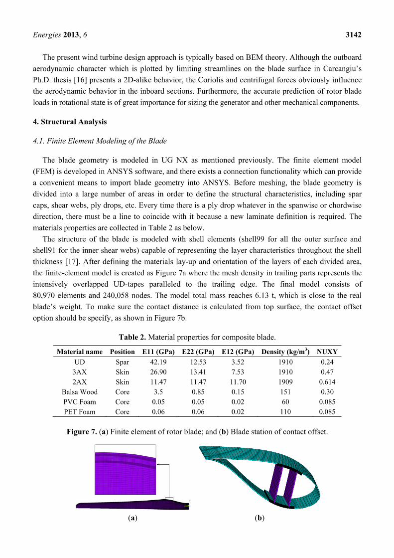
The structure of the blade is modeled with shell elements (shell99 for all the outer surface and

shell91 for the inner shear webs) capable of representing the layer characteristics throughout the shell

thickness [17]. After defining the materials lay-up and orientation of the layers of each divided area,

the finite-element model is created as Figure 7a where the mesh density in trailing parts represents the

intensively overlapped UD-tapes paralleled to the trailing edge. The final model consists of

80,970 elements and 240,058 nodes. The model total mass reaches 6.13 t, which is close to the real

blade’s weight. To make sure the contact distance is calculated from top surface, the contact offset

option should be specify, as shown in Figure 7b.

Table 2. Material properties for composite blade.

Material name Position E11 (GPa) E22 (GPa) E12 (GPa) Density (kg/m3) NUXY

UD Spar 42.19 12.53 3.52 1910 0.24 3AX Skin 26.90 13.41 7.53 1910 0.47 2AX Skin 11.47 11.47 11.70 1909 0.614

Balsa Wood Core 3.5 0.85 0.15 151 0.30 PVC Foam Core 0.05 0.05 0.02 60 0.085 PET Foam Core 0.06 0.06 0.02 110 0.085

Figure 7. (a) Finite element of rotor blade; and (b) Blade station of contact offset.

(a) (b)

Energies 2013, 6 3143

4.2. Dynamic Behavior

As one of the most complex stress parts of a wind turbine, the blade is under coupled processes of

aerodynamic, inertia and elasticity forces. When the natural frequency of blade is the same as the

frequency of exciting forces, resonance is produced. To avoid resonance, frequencies must be

staggered in the mainly operation intervals. Therefore, the accurate calculates of the nature frequency

of blade are of great importance. Usually, these dynamic characteristics are determined for the lowest

3–4 flexural bending modes and for the first torsional mode [18]. The 1.5 MW rotor blade has already

been validated by the China Classification Society. The deviation between experimental results and the

results from the FE-model is seen in Table 3.

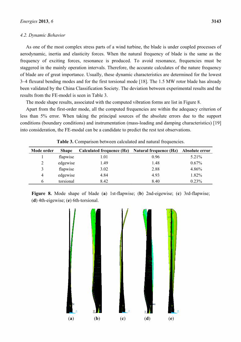
The mode shape results, associated with the computed vibration forms are list in Figure 8.

Apart from the first-order mode, all the computed frequencies are within the adequacy criterion of

less than 5% error. When taking the principal sources of the absolute errors due to the support

conditions (boundary conditions) and instrumentation (mass-loading and damping characteristics) [19]

into consideration, the FE-modal can be a candidate to predict the rest test observations.

Table 3. Comparison between calculated and natural frequencies.

Mode order Shape Calculated frequence (Hz) Natural frequence (Hz) Absolute error

1 flapwise 1.01 0.96 5.21% 2 edgewise 1.49 1.48 0.67% 3 flapwise 3.02 2.88 4.86% 4 edgewise 4.84 4.93 1.82% 6 torsional 8.42 8.40 0.23%

Figure 8. Mode shape of blade (a) 1st-flapwise; (b) 2nd-eigewise; (c) 3rd-flapwise;

(d) 4th-eigewise; (e) 6th-torsional.

(a) (b) (c) (d) (e)

Energies 2013, 6 3144

4.3. Static Analysis under Limit Load

For the structural-response analysis, peak loads are derived by considering a 50-year extreme gust

of 59 m/s [14] with the pitch of the blade adjusted to obtain the wind attack-angle associated with the

largest aerodynamic loads. The limit CFD loads of the rotor blade are obtained using CFD method

mentioned in Section 3.

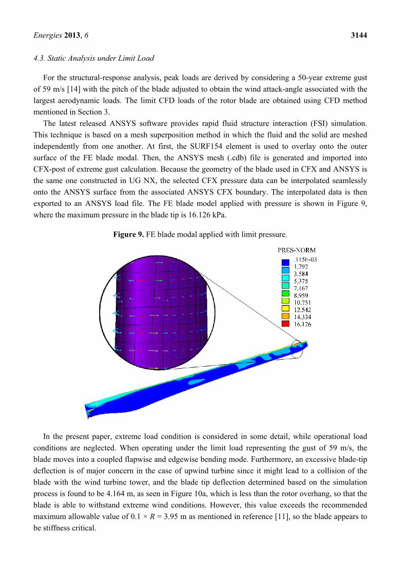
The latest released ANSYS software provides rapid fluid structure interaction (FSI) simulation.

This technique is based on a mesh superposition method in which the fluid and the solid are meshed

independently from one another. At first, the SURF154 element is used to overlay onto the outer

surface of the FE blade modal. Then, the ANSYS mesh (.cdb) file is generated and imported into

CFX-post of extreme gust calculation. Because the geometry of the blade used in CFX and ANSYS is

the same one constructed in UG NX, the selected CFX pressure data can be interpolated seamlessly

onto the ANSYS surface from the associated ANSYS CFX boundary. The interpolated data is then

exported to an ANSYS load file. The FE blade model applied with pressure is shown in Figure 9,

where the maximum pressure in the blade tip is 16.126 kPa.

Figure 9. FE blade modal applied with limit pressure.

In the present paper, extreme load condition is considered in some detail, while operational load

conditions are neglected. When operating under the limit load representing the gust of 59 m/s, the

blade moves into a coupled flapwise and edgewise bending mode. Furthermore, an excessive blade-tip

deflection is of major concern in the case of upwind turbine since it might lead to a collision of the

blade with the wind turbine tower, and the blade tip deflection determined based on the simulation

process is found to be 4.164 m, as seen in Figure 10a, which is less than the rotor overhang, so that the

blade is able to withstand extreme wind conditions. However, this value exceeds the recommended

maximum allowable value of 0.1 × R = 3.95 m as mentioned in reference [11], so the blade appears to

be stiffness critical.

Energies 2013, 6 3145

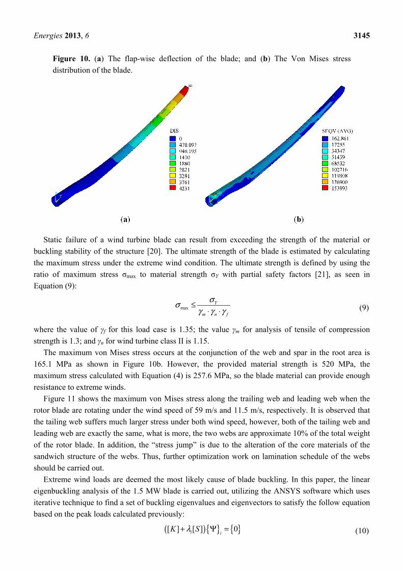
Figure 10. (a) The flap-wise deflection of the blade; and (b) The Von Mises stress

distribution of the blade.

Static failure of a wind turbine blade can result from exceeding the strength of the material or

buckling stability of the structure [20]. The ultimate strength of the blade is estimated by calculating

the maximum stress under the extreme wind condition. The ultimate strength is defined by using the

ratio of maximum stress σmax to material strength σY with partial safety factors [21], as seen in

Equation (9):

maxY

m n f

σσγ γ γ

≤⋅ ⋅

(9)

where the value of γf for this load case is 1.35; the value γm for analysis of tensile of compression

strength is 1.3; and γn for wind turbine class II is 1.15.

The maximum von Mises stress occurs at the conjunction of the web and spar in the root area is

165.1 MPa as shown in Figure 10b. However, the provided material strength is 520 MPa, the

maximum stress calculated with Equation (4) is 257.6 MPa, so the blade material can provide enough

resistance to extreme winds.

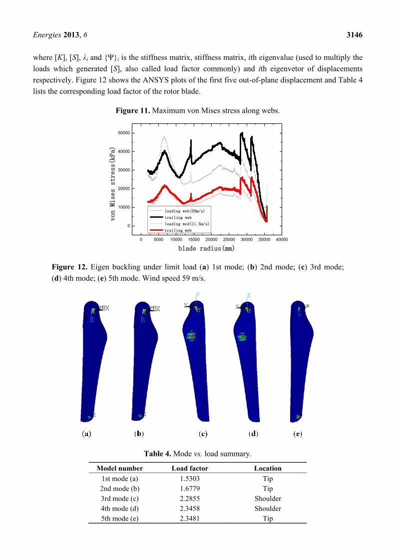
Figure 11 shows the maximum von Mises stress along the trailing web and leading web when the

rotor blade are rotating under the wind speed of 59 m/s and 11.5 m/s, respectively. It is observed that

the tailing web suffers much larger stress under both wind speed, however, both of the tailing web and

leading web are exactly the same, what is more, the two webs are approximate 10% of the total weight

of the rotor blade. In addition, the “stress jump” is due to the alteration of the core materials of the

sandwich structure of the webs. Thus, further optimization work on lamination schedule of the webs

should be carried out.

Extreme wind loads are deemed the most likely cause of blade buckling. In this paper, the linear

eigenbuckling analysis of the 1.5 MW blade is carried out, utilizing the ANSYS software which uses

iterative technique to find a set of buckling eigenvalues and eigenvectors to satisfy the follow equation

based on the peak loads calculated previously:

( ) [ ] [ ] 0i iK Sλ+ Ψ = (10)

Energies 2013, 6 3146

where [K], [S], λi and Ψi is the stiffness matrix, stiffness matrix, ith eigenvalue (used to multiply the

loads which generated [S], also called load factor commonly) and ith eigenvetor of displacements

respectively. Figure 12 shows the ANSYS plots of the first five out-of-plane displacement and Table 4

lists the corresponding load factor of the rotor blade.

Figure 11. Maximum von Mises stress along webs.

0 5000 10000 15000 20000 25000 30000 35000 40000

0

10000

20000

30000

40000

50000

von

Mis

es s

tres

s(kP

a)

blade radius(mm)

leading web(59m/s)

trailing web

leading wed(11.5m/s)

trailing web

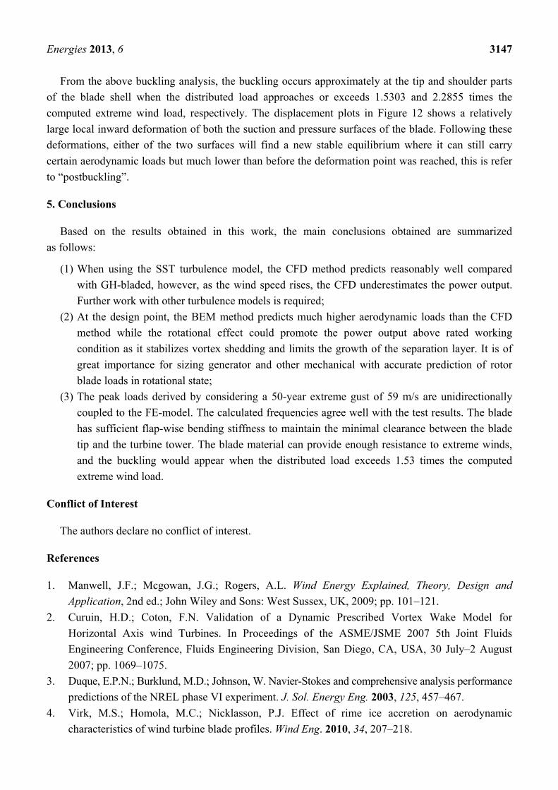
Figure 12. Eigen buckling under limit load (a) 1st mode; (b) 2nd mode; (c) 3rd mode;

(d) 4th mode; (e) 5th mode. Wind speed 59 m/s.

Table 4. Mode vs. load summary.

Model number Load factor Location

1st mode (a) 1.5303 Tip 2nd mode (b) 1.6779 Tip 3rd mode (c) 2.2855 Shoulder 4th mode (d) 2.3458 Shoulder 5th mode (e) 2.3481 Tip

Energies 2013, 6 3147

From the above buckling analysis, the buckling occurs approximately at the tip and shoulder parts

of the blade shell when the distributed load approaches or exceeds 1.5303 and 2.2855 times the

computed extreme wind load, respectively. The displacement plots in Figure 12 shows a relatively

large local inward deformation of both the suction and pressure surfaces of the blade. Following these

deformations, either of the two surfaces will find a new stable equilibrium where it can still carry

certain aerodynamic loads but much lower than before the deformation point was reached, this is refer

to “postbuckling”.

5. Conclusions

Based on the results obtained in this work, the main conclusions obtained are summarized

as follows:

(1) When using the SST turbulence model, the CFD method predicts reasonably well compared

with GH-bladed, however, as the wind speed rises, the CFD underestimates the power output.

Further work with other turbulence models is required;

(2) At the design point, the BEM method predicts much higher aerodynamic loads than the CFD

method while the rotational effect could promote the power output above rated working

condition as it stabilizes vortex shedding and limits the growth of the separation layer. It is of

great importance for sizing generator and other mechanical with accurate prediction of rotor

blade loads in rotational state;

(3) The peak loads derived by considering a 50-year extreme gust of 59 m/s are unidirectionally

coupled to the FE-model. The calculated frequencies agree well with the test results. The blade

has sufficient flap-wise bending stiffness to maintain the minimal clearance between the blade

tip and the turbine tower. The blade material can provide enough resistance to extreme winds,

and the buckling would appear when the distributed load exceeds 1.53 times the computed

extreme wind load.

Conflict of Interest

The authors declare no conflict of interest.

References

1. Manwell, J.F.; Mcgowan, J.G.; Rogers, A.L. Wind Energy Explained, Theory, Design and

Application, 2nd ed.; John Wiley and Sons: West Sussex, UK, 2009; pp. 101–121.

2. Curuin, H.D.; Coton, F.N. Validation of a Dynamic Prescribed Vortex Wake Model for

Horizontal Axis wind Turbines. In Proceedings of the ASME/JSME 2007 5th Joint Fluids

Engineering Conference, Fluids Engineering Division, San Diego, CA, USA, 30 July–2 August

2007; pp. 1069–1075.

3. Duque, E.P.N.; Burklund, M.D.; Johnson, W. Navier-Stokes and comprehensive analysis performance

predictions of the NREL phase VI experiment. J. Sol. Energy Eng. 2003, 125, 457–467.

4. Virk, M.S.; Homola, M.C.; Nicklasson, P.J. Effect of rime ice accretion on aerodynamic

characteristics of wind turbine blade profiles. Wind Eng. 2010, 34, 207–218.

Energies 2013, 6 3148

5. Keck, R.-E. A numerical investigation of nacelle anemometry for a HAWT using actuator disc

and line models in CFX. Renew. Energy 2012, 48, 72–84.

6. Wuchner, R.; Kupzok, A.; Bletzinger, K.U. A framework for stabilized partitioned analysis of

thin membrane-wind interaction. Int. J. Mumer. Methods Fluids 2007, 54, 945–963.

7. Jensen, F.M.; Falzon, B.G.; Ankersen, J.; Stang, H. Structural testing and numerical simulation of

a 34 m composite wind turbine blade. Compos. Struct. 2006, 76, 52–61.

8. Hermann, T.M.; Mamarthupatti, D.; Locke, J.E. Postbuckling analysis of a wind turbine blade

substructure. J. Sol. Energy Eng. 2005, 127, 262–280.

9. Rajadurai, J.S.; Christopher, T.; Thanigaiyarasu, G.; Nageswara Rao, B. Finite element analysis with

an improved failure criterion for composite wind turbine blades. Forsch. Ing. 2008, 72, 193–207.

10. Grujicic, M.; Arakere, G.; Sellappan, V.; Vallejo, A.; Ozen, M. Structural-response analysis,

fatigue-life prediction and material selection for 1 MW horizontal-axis wind-turbine blades.

J. Mater. Eng. Perform. 2010, 19, 780–801.

11. Grujicic, M.; Arakere, G.; Pandurangan, B.; Sellappan, V.; Vallejo, A.; Ozen, M. Multidisciplinary

optimization for fiber-glass reinforced epoxy-matrix composite 5 MW horizontal-axis wind-turbine

blades. J. Mater. Eng. Perform. 2010, 19, 1116–1127.

12. Sutherland, H.J. On the Fatigue Analysis of Wind Turbines; SANDA99-0089; Sandia National

Laboratories: Albuquerque, NM, USA, 1999.

13. Menter, F.R.; Kuntz, M.; Langtry, R. Ten years of industrial experience with the SST turbulence

model. Heat Mass Transf. 2003, 4, 625–632.

14. International Electrotechnical Commission. IEC International Standard 61400-1, Part I: Design

Requirements, 3rd ed.; International Electrotechnical Commission: Geneva, Switzerland, 2005.

15. Cimbala, J.M. Introduction to Computational Fluid Dynamics, 2nd ed.; Penn State University:

University Park, PA, USA, 2012.

16. Carcangiu, C.E. CFD-RANS Study of Horizontal Axis Wind Turbines. Ph.D. Thesis, University

of Cagliari, Cagliari, Italy, 2008.

17. McKittrick, L.R.; Cairns, D.S.; Mandell, J.; Combs, D.C.; Rabern, D.A.; VanLuchene, D.V.

Analysis of a Composite Blade Design for the AOC 15/50 Wind Turbine Using a Finite Element

Model; SAND 2001–1441; Sandia National Laboratories: Albuquerque, NM, USA, 2001.

18. Larsen, G.C.; Hansen, M.H.; Baumgart, A.; Carlén, I. Modal Analysis of Wind Turbine Blades;

Risø National Laboratory: Roskilde, Denmark, 2002.

19. Todd, G.D.; Carne, T. Experimental modal analysis of research-sized wind turbine blades. Sound

Vib. 2010, 44, 8–11.

20. Bir, G.; Migliore, P. A Computerized Method for Preliminary Structural Design of Composite

Wind Turbine Blades; AIAA-2001-0022; National Wind Technology Center, National Renewable

Energy Laboratory: Golden, CO, USA, 2001.

21. Hu, W.F.; Han, I.; Park, S.C.; Choi, D.H. Multi-objective structural optimization of a HAWT

composite blade based on ultimate limit state analysis. J. Mech. Sci. Technol. 2012, 26, 129–135.

© 2013 by the authors; licensee MDPI, Basel, Switzerland. This article is an open access article

distributed under the terms and conditions of the Creative Commons Attribution license

(http://creativecommons.org/licenses/by/3.0/).