Enabling scalable and accurate clustering of...
23
Parallel Computing 63 (2017) 38–60 Contents lists available at ScienceDirect Parallel Computing journal homepage: www.elsevier.com/locate/parco Enabling scalable and accurate clustering of distributed ligand geometries on supercomputers Boyu Zhang a,b , Trilce Estrada c , Pietro Cicotti d , Pavan Balaji e , Michela Taufer a,∗ a University of Delaware, 210 South College Ave. Newark, DE 19716, USA b Purdue University, 610 Purdue Mall, West Lafayette, IN 47907, USA c University of New Mexico, 1155 University Blvd. SE. Albuquerque, NM 87106, USA d San Diego Supercomputer Center, 9500 Gilman Drive | La Jolla, CA 92093, USA e Argonne National Laboratory, 9700 Cass Ave, Lemont, IL 60439, USA a r t i c l e i n f o Article history: Received 15 March 2016 Revised 26 November 2016 Accepted 28 February 2017 Available online 1 March 2017 Keywords: Ligand conformations Protein-ligand docking Drug design Octree-based clustering N-dimensional clustering In situ analytics a b s t r a c t We present an efficient and accurate clustering method for the analysis of protein-ligand docking datasets on large distributed-memory systems. For each ligand conformation in the dataset, our clustering algorithm first extracts relevant geometrical properties and transforms the properties into a single metadata point in the N-dimensional (N-D) space. Then, it performs an N-D clustering on the metadata to search for predominant clusters. Our method avoids the need to move ligand conformations among nodes, because it ex- tracts relevant data properties locally and concurrently. By doing so, we transform the analysis problem (e.g., clustering or classification) into a search for property aggregates. Our analysis shows that when using small computer systems of up to 64 nodes, the per- formance is not sensitive to data content and distribution. When using larger computer systems of up to 256 nodes the scalability of simulations with strong convergence to- ward specific geometries is less sensitive to overheads due to the shuffling of metadata information. We also demonstrate that our method of metadata extraction captures the geometrical properties of ligand conformations more effectively and clusters and predicts near-native ligand conformations more accurately than do traditional methods, including the hierarchical clustering and energy-based scoring methods. © 2017 Elsevier B.V. All rights reserved. 1. Introduction In studies of disease processes, a common problem involves the search for small molecules (ligands) that can interact with a larger molecule, such as a protein, that is involved in a disease state. Specifically, when ligands dock well in a protein, they can potentially be used as a drug to stop or prevent diseases associated with the protein malfunction. The study of the docking process is computationally performed with docking simulations, which consist of sequences of independent docking trials. Each docking trial generates a series of random initial ligand conformations and orientations. These conformations can be docked into the protein-binding site (or pocket) through molecular dynamics simulated annealing [1]. Since the process is highly parallelizable, it is efficiently performed on distributed-memory systems (e.g., supercomputers and volunteer com- puting platforms), resulting in a distributed collection of hundreds of thousands of ligand conformations across the nodes ∗ Corresponding author. E-mail address: [email protected] (M. Taufer). http://dx.doi.org/10.1016/j.parco.2017.02.005 0167-8191/© 2017 Elsevier B.V. All rights reserved.
Transcript of Enabling scalable and accurate clustering of...
Parallel Computing 63 (2017) 38–60
Contents lists available at ScienceDirect
Parallel Computing
journal homepage: www.elsevier.com/locate/parco
Enabling scalable and accurate clustering of distributed ligand
geometries on supercomputers
Boyu Zhang
a , b , Trilce Estrada
c , Pietro Cicotti d , Pavan Balaji e , Michela Taufer a , ∗
a University of Delaware, 210 South College Ave. Newark, DE 19716, USA b Purdue University, 610 Purdue Mall, West Lafayette, IN 47907, USA c University of New Mexico, 1155 University Blvd. SE. Albuquerque, NM 87106, USA d San Diego Supercomputer Center, 9500 Gilman Drive | La Jolla, CA 92093, USA e Argonne National Laboratory, 9700 Cass Ave, Lemont, IL 60439, USA
a r t i c l e i n f o
Article history:
Received 15 March 2016
Revised 26 November 2016
Accepted 28 February 2017
Available online 1 March 2017
Keywords:
Ligand conformations
Protein-ligand docking
Drug design
Octree-based clustering
N-dimensional clustering
In situ analytics
a b s t r a c t
We present an efficient and accurate clustering method for the analysis of protein-ligand
docking datasets on large distributed-memory systems. For each ligand conformation in
the dataset, our clustering algorithm first extracts relevant geometrical properties and
transforms the properties into a single metadata point in the N-dimensional (N-D) space.
Then, it performs an N-D clustering on the metadata to search for predominant clusters.
Our method avoids the need to move ligand conformations among nodes, because it ex-
tracts relevant data properties locally and concurrently. By doing so, we transform the
analysis problem (e.g., clustering or classification) into a search for property aggregates.
Our analysis shows that when using small computer systems of up to 64 nodes, the per-
formance is not sensitive to data content and distribution. When using larger computer
systems of up to 256 nodes the scalability of simulations with strong convergence to-
ward specific geometries is less sensitive to overheads due to the shuffling of metadata
information. We also demonstrate that our method of metadata extraction captures the
geometrical properties of ligand conformations more effectively and clusters and predicts
near-native ligand conformations more accurately than do traditional methods, including
the hierarchical clustering and energy-based scoring methods.
© 2017 Elsevier B.V. All rights reserved.
1. Introduction
In studies of disease processes, a common problem involves the search for small molecules (ligands) that can interact
with a larger molecule, such as a protein, that is involved in a disease state. Specifically, when ligands dock well in a protein,
they can potentially be used as a drug to stop or prevent diseases associated with the protein malfunction. The study of the
docking process is computationally performed with docking simulations, which consist of sequences of independent docking
trials. Each docking trial generates a series of random initial ligand conformations and orientations. These conformations can
be docked into the protein-binding site (or pocket) through molecular dynamics simulated annealing [1] . Since the process
is highly parallelizable, it is efficiently performed on distributed-memory systems (e.g., supercomputers and volunteer com-
puting platforms), resulting in a distributed collection of hundreds of thousands of ligand conformations across the nodes
∗ Corresponding author.
E-mail address: [email protected] (M. Taufer).
http://dx.doi.org/10.1016/j.parco.2017.02.005
0167-8191/© 2017 Elsevier B.V. All rights reserved.
B. Zhang et al. / Parallel Computing 63 (2017) 38–60 39
Fig. 1. Overview of ligand clustering in which ligand conformations are mapped into metadata of 3-D points and metadata points are searched for knowl-
edge acquisition.
of the system. The docking simulations often produce large datasets of ligand conformations that naturally converge toward
native conformations (i.e., conformations experimentally observed).
When analyzing large datasets searching for the native conformations, a common practice is to reduce the number of
candidates up to 100 conformations based on energy values and then leave the scientists with the tedious task of subjec-
tively selecting a possible near-native ligand. Scientists normally perform this task manually by using visual tools such as
VMD [2] or Chimera [3] . Then the scientists perform wet-lab high-throughput screening on the selected ligands. Not only
does the manual selection process still depend on inaccurate energy scoring but it also can be highly error-prone. To the
best of our knowledge, most advanced methods of handling this task are not fully automated, and the need remains not
only for automation of this process but also for faster selecting methodology.
In previous work [4] , we addressed the problem of accurately and automatically selecting near-native conformations
from the dataset by using a probabilistic hierarchical clustering based on ligand geometries. Unfortunately the method in
[4] requires direct comparison of the conformations’ geometries iteratively. When very large numbers of conformations are
distributed across a large number of nodes of the distributed-memory system, the movement and comparison of data can
have a significant negative impact on the performance and scalability of the analysis.
In this paper we move away from the iterative process used in [4] and propose a more efficient and accurate method to
cluster conformation geometries across the nodes of a distributed-memory system that does not require direct movement
and comparison of ligand conformations. The method used in this paper was initially presented in [5–7] . This paper gath-
ers the contributions of the publications in a comprehensive manuscript. More important, this paper substantially extends
performance results presented at the IEEE International Scalable Computing Challenge (SCALE 2015) [7] and adds accuracy
results not presented before.
Our method first maps the relevant geometrical properties of each conformation into a concise metadata point in the
N-dimensional (or N-D) space (i.e., a single point in a lower-dimensional space). Our lower-dimensional representation can
be viewed as metadata since it encodes the geometries of the original ligand conformations. The geometrical properties
quantify the direction and position of the ligand confirmations in the fixed, known docking pocket of the protein. Then,
our method performs an N-D clustering on all metadata points to search for dense clusters. Our hypothesis is that the
method accurately maps ligand conformations with similar geometries to metadata in the N-D space in close proximity.
Thus subspaces of the metadata space with higher point concentrations (or densities) can be associated with most frequently
found ligand conformations in a docking simulation that naturally converges toward the native conformation. For mapping
conformation geometries into metadata points, we consider three variations of an algorithm that uses projections and linear
interpolations into 3-D, 3-Dlog, and 6-D mappings. To search for the densest and deeper subspace in the N-D space of
metadata points, we consider two variations of an N-D tree search. In the first variation, called GlobalToLocal (GL), the
extracted properties are moved across nodes to build a global view of the dataset; these properties are iteratively and locally
analyzed while searching for some class or cluster convergence. In the second variation, called LocalToGlobal (LG), partial
properties are analyzed locally on each node to generate a property aggregate, which is a scalar number that summarizes
local properties of the data. In this variation, instead of exchanging extracted properties, LG exchanges only a few scalar
property aggregates across the nodes. Both approaches are based on the general theme of moving computation to the data.
Fig. 1 shows an overview of our approach for one of the three variations for mapping conformation geometries in which each
conformation geometry is mapped into a single 3-D point and the N-D search is performed on an octree. By mapping atomic
coordinates of a ligand into a single-point metadata, our clustering method enables in situ analysis of ligand conformations
40 B. Zhang et al. / Parallel Computing 63 (2017) 38–60
in protein-ligand docking simulations due to the following three aspects: our clustering method executes sufficiently fast
comparing to the docking simulation, it avoids moving actual ligand coordinates data, and it limits the memory use of
ligand conformations by keeping only 3-D or 6-D metadata points in memory.
Our performance study assesses our method at both small and large scales. At the small scale (up to 64 compute nodes),
we measure the performance of the GL and LG variations and assess their sensitivity to both logical and physical data
distributions. Because we discovered that the GL variation exhibits poor scalability already on a cluster of 64 compute
nodes, we focus our present study at the larger scale (up to 256 nodes) on the LocalToGlobal variation only and identify the
crucial features in a logical distribution that more significantly impact the execution times when performing the search on
large datasets of ligand conformations.
Our accuracy study aims to quantify the capability of our proposed mapping variations (i.e., the 3-D, 3-Dlog, and 6-D
mappings) to capture and preserve ligand conformation geometries. In other words, we assess whether our transformation
of conformations into simple metadata points preserves the knowledge of the conformations geometries and to determine
whether we can still acquire this knowledge from the most frequently sampled geometries despite their generation across
multiple nodes of a distributed-memory system. To this end we analyze the ligand conformations generated by real large-
scale protein-ligand docking simulations within the Docking@Home project. This project considers a diverse set of proteins
and ligands from the LPDB database and performs extensive docking attempts [8] .
The paper is organized as follows. Section 2 gives the background knowledge on protein-ligand docking simulations.
Section 3 reviews related work on the clustering techniques of ligand conformations and the distributed clustering using
MapReduce. Section 4 discusses our method and its variations of mapping and N-D search. Sections 5 and 6 present the
performance and accuracy evaluations, respectively. Section 7 summarizes our conclusions and briefly describes future work.
2. Background
This section provides a comprehensive view of the science that is enabled by our scalable and accurate clustering method
as well as a short overview of the MapReduce paradigm.
2.1. Protein-ligand docking
Techniques for performing protein-ligand docking simulations on clusters and supercomputers are diverse. In this paper,
the docking algorithms we consider are based on Classical Molecular Dynamics simulations. An extensive survey of docking
techniques is not in the scope of this paper and can be found in [9] . Computationally, a protein-ligand docking simulations
seeks to find near-native ligand conformations in a large dataset of conformations docked in a protein [10] . A conforma-
tion is considered near-native if the root-mean-square deviation (RMSD) of the heavy atom coordinates is smaller than or
equal to two Angstroms from the experimentally observed conformation. Algorithmically, a docking simulation consists of a
sequence of independent docking trials. An independent docking trial starts by generating a series of random initial ligand
conformations; each conformation is given multiple random orientations. The resulting conformations are docked into the
protein-binding site. Hundreds of thousands of docking attempts are performed concurrently. Molecular dynamics simulated
annealing is used to search for low-energy conformations of the ligand on the protein pocket.
The docking process is only one of the key steps. Once the results (ligand conformations) are collected, they need to
be evaluated to predict the near-native ligand geometry. Traditionally, docked conformations with minimum energy are
assumed to be near-native. Research has shown, however, that this is not always the case [5] . Since selecting the near-
native ligand geometry based on energy alone may result in incorrect conclusions, an alternative approach selects the near-
native geometry from clustering. In previous work we showed that compact clusters of docked conformations grouped by
their geometries are more likely to be near-native than are the individual conformations with lowest energy [5,11] . Large
numbers of ligand conformations were sampled through the Docking@Home (D@H) project in the past five years and are
used here as the dataset of interest. Hundreds of millions of docked ligand conformations must be compared with each
other in terms of their geometries. However, this approach can result in extensive computing and storage needs. Ideally the
clustering methods have to be scalable, efficient, and accurate, allowing scientists to compare and select across a large set
of docking results.
2.2. Generating large datasets with Docking@Home
Although the system software for generating the large datasets of conformations used for our analysis is not our key
contribution here, we briefly describe how we collect the docking data for this study using the Docking@Home project [12] .
Docking@Home is one of the many computational molecular docking approaches for sampling large conformational spaces
of ligands that have been used for virtual screening [13–15] . Typically a given docking method is evaluated with a selected
number of experimentally determined protein-ligand complexes. In general, docking methods differ from each other in the
algorithm used in the conformational search [16,17] , the scoring function used to predict ligand geometries, and the scoring
function used to rank compounds (or predict DGbinding) [18] .
Docking@Home (D@H) uses the Volunteer Computing (VC) programming model to build the framework of distributed
computing resources for the docking simulations; ordinary people volunteer processing and storage resources across the
B. Zhang et al. / Parallel Computing 63 (2017) 38–60 41
Internet to contribute to the scientific simulations. D@H builds on top of Berkeley Open Infrastructure for Network Com-
puting (BOINC) [19] , well-known VC middleware. D@H computationally searches for potential drug-like molecules against
diseases such as breast cancer and HIV. D@H generates a large space of possible docking conformations. In order to exten-
sively search this space, millions of independent docking attempts (jobs) are processed by the D@H server, which distributes
them to clients across the Internet for computation. Computers from volunteers perform the docking simulation and return
results consisting of the docked 3-D ligand conformation and its associated energy values.
To explore the conformational space of the ligands, D@H considers a representation of the solvent by using two docking
methods: (1) an implicit representation of water using a distance-dependent dielectric coefficient (low if the atoms are close
and progressively larger as the interatom distance increases) and (2) a more physically accurate implicit representation of
water using a generalized Born model [20] . The latter is a more compute- and memory-intensive method, but it provides a
more physically accurate description of the potential energy of a ligand where part of the ligand conformation is exposed to
solvent. In many such situations, the generalized Born model should help provide better ligand conformation; for example,
when one orientation of a given ligand leaves a large bulky hydrophobic group exposed to solvent, this is penalized, whereas
exposing a hydrophilic group such as a hydroxyl group to solvent is much more favorable.
The molecular docking is performed by using the CHARMM (Chemistry at HARvard Molecular Mechanics) molecular sim-
ulation package [21] and an intermediate-accuracy all-atom force field. The CHARMM script describing the docking process
considers a protein-ligand complex as a composition of a flexible ligand and a rigid protein structure (i.e., on a three-
dimensional lattice of regularly spaced points surrounding and centered on the active site of the protein, where each point
on the grid stores the potential energy of a “probe” atom’s interaction with the molecule). A D@H simulation consists of a
sequence of independent trials (or jobs). For each trial, either a randomly generated conformation or a user-defined con-
formation for a ligand is used as initial conformation. Random conformations are generated starting from the ligand crystal
structure with random initial velocities on each ligand atom. Then the initial conformation is randomly rotated to produce
a set of orientations that are placed into the active site of the protein or docking pocket (docking attempts).
Once the ligand is docked into the protein site, a molecular dynamics simulation is performed consisting of a gradual
heating phase of 40 0 0 1 fs (femtosecond) steps from 300 K to 700 K, followed by a cooling phase of 10,0 0 0 1 fs steps back
to 300 K. In order to facilitate the penetration of ligands into protein sites and allow larger conformational changes, van der
Waals (vdW) and electrostatic potentials with soft-core repulsions are utilized. A soft-core repulsion reduces the potential
barrier at vanishing interatomic distances to a finite limit, allowing ligands to pass between conformational minima with a
relatively small potential barrier that normally is large and impossible to overcome with an unmodified standard potential.
The detailed description of the docking method and its comparison with other docking codes are not in the current scope
of this work; details can be found in [1,22] . Once the results (ligand conformations) are collected, they need to be scored.
Initially D@H used an energy-based scoring method; our previous work pointed out how this scoring approach can result
in incorrect conclusions because energy values are approximated by the simplified methods used in the computational
algorithms. The alternative approach we pursue scores ligands based on the geometry of their resulting conformations.
2.3. Semi- and fully decentralized memory systems
The data considered here comprises a large number of individual data records and is distributed across the nodes of a
large distributed-memory system. More specifically, we consider semi- and fully decentralized distributed-memory systems.
In a semi-decentralized system, processes report to more than one node, usually to the closest one in the cluster’s network
topology, and take advantage of locality by reducing expensive data transfer and potential storage pressure. In contrast, in
a fully decentralized system, each node stores its own data, which reduces the need for data transfers and increases the
amount of locally stored data. Logically, the entire dataset can converge toward one or multiple scientific properties, or it
may not convey any scientific information. Physically, data with similar scientific properties may agglomerate in topologi-
cally close nodes or may be dispersed across nodes. Logical and physical tendencies are not known a priori when data is
generated in semi- or fully decentralized systems. In general, scientists must move data across nodes in order to analyze and
understand it. This process can be extremely costly in terms of execution time. For completeness, we define three scenarios
that resemble the challenging conditions faced by scientists when dealing with distributed systems with large amounts of
data. The scenarios consist of data distributed as follows:
• a semi-decentralized manner in which data with similar properties are generated by and stored in specific nodes; • a fully decentralized, synchronous manner in which data is gathered at regular intervals producing a uniform distribution
of data properties across the nodes in a round-robin fashion; and
• a fully decentralized, asynchronous manner in which every node acts by itself and properties are stored randomly across
nodes.
2.4. MapReduce-MPI and other MapReduce libraries
MapReduce-MPI is a runtime library supporting the MapReduce programming model [23] . It is written in C++ and MPI.
It runs a MapReduce program using a number of MPI processes, the number of which is defined by the programmer. Each
process runs both the map and the reduce functions. It first runs the map function on partial data and outputs the inter-
mediate 〈 key, value 〉 pairs in parallel. Then, the MapReduce-MPI framework communicates all the values with the same key
42 B. Zhang et al. / Parallel Computing 63 (2017) 38–60
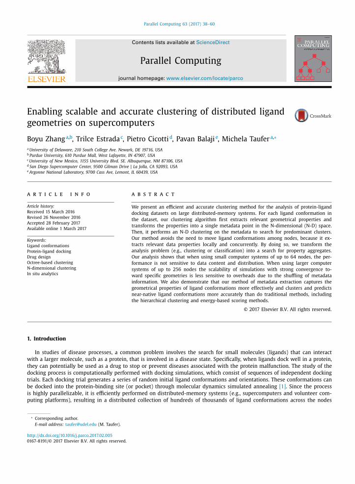
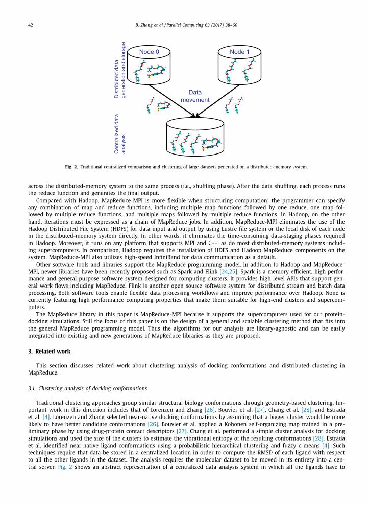
Fig. 2. Traditional centralized comparison and clustering of large datasets generated on a distributed-memory system.
across the distributed-memory system to the same process (i.e., shuffling phase). After the data shuffling, each process runs
the reduce function and generates the final output.
Compared with Hadoop, MapReduce-MPI is more flexible when structuring computation: the programmer can specify
any combination of map and reduce functions, including multiple map functions followed by one reduce, one map fol-
lowed by multiple reduce functions, and multiple maps followed by multiple reduce functions. In Hadoop, on the other
hand, iterations must be expressed as a chain of MapReduce jobs. In addition, MapReduce-MPI eliminates the use of the
Hadoop Distributed File System (HDFS) for data input and output by using Lustre file system or the local disk of each node
in the distributed-memory system directly. In other words, it eliminates the time-consuming data-staging phases required
in Hadoop. Moreover, it runs on any platform that supports MPI and C++, as do most distributed-memory systems includ-
ing supercomputers. In comparison, Hadoop requires the installation of HDFS and Hadoop MapReduce components on the
system. MapReduce-MPI also utilizes high-speed InfiniBand for data communication as a default.
Other software tools and libraries support the MapReduce programming model. In addition to Hadoop and MapReduce-
MPI, newer libraries have been recently proposed such as Spark and Flink [24,25] . Spark is a memory efficient, high perfor-
mance and general purpose software system designed for computing clusters. It provides high-level APIs that support gen-
eral work flows including MapReduce. Flink is another open source software system for distributed stream and batch data
processing. Both software tools enable flexible data processing workflows and improve performance over Hadoop. None is
currently featuring high performance computing properties that make them suitable for high-end clusters and supercom-
puters.
The MapReduce library in this paper is MapReduce-MPI because it supports the supercomputers used for our protein-
docking simulations. Still the focus of this paper is on the design of a general and scalable clustering method that fits into
the general MapReduce programming model. Thus the algorithms for our analysis are library-agnostic and can be easily
integrated into existing and new generations of MapReduce libraries as they are proposed.
3. Related work
This section discusses related work about clustering analysis of docking conformations and distributed clustering in
MapReduce.
3.1. Clustering analysis of docking conformations
Traditional clustering approaches group similar structural biology conformations through geometry-based clustering. Im-
portant work in this direction includes that of Lorenzen and Zhang [26] , Bouvier et al. [27] , Chang et al. [28] , and Estrada
et al. [4] . Lorenzen and Zhang selected near-native docking conformations by assuming that a bigger cluster would be more
likely to have better candidate conformations [26] . Bouvier et al. applied a Kohonen self-organizing map trained in a pre-
liminary phase by using drug-protein contact descriptors [27] . Chang et al. performed a simple cluster analysis for docking
simulations and used the size of the clusters to estimate the vibrational entropy of the resulting conformations [28] . Estrada
et al. identified near-native ligand conformations using a probabilistic hierarchical clustering and fuzzy c-means [4] . Such
techniques require that data be stored in a centralized location in order to compute the RMSD of each ligand with respect
to all the other ligands in the dataset. The analysis requires the molecular dataset to be moved in its entirety into a cen-
tral server. Fig. 2 shows an abstract representation of a centralized data analysis system in which all the ligands have to
B. Zhang et al. / Parallel Computing 63 (2017) 38–60 43
be moved to a local storage where they can be compared and clustered. The fully centralized approach is not scalable and
can result in serious storage and bandwidth pressures on the server. Thus, the challenge involves ways to find these dense
ligand clusters of geometric representations efficiently, especially when the data is acquired in a distributed way. While each
conformation is small (on the order of 10 Kbytes), the number of conformations that must be moved across the distributed-
memory system and compared is extremely large; depending on the type and number of proteins, the conformation dataset
can comprise tens or hundreds of millions of ligands. This scenario is expected when thousands of processes perform in-
dividual docking simulations and store their results locally. As an example, consider the D@H project that is supported
by more than 188,0 0 0 hosts. If all the hosts communicate their local results to a centralized server simultaneously, even
when each host communicates data in terms of 100 ligand conformations (i.e., around 7 MB), the data sending across the
distributed-memory system is more than 1 TB.
To avoid this big data movement among nodes, in previous work our group proposed a distributed clustering method
in MapReduce that first extracts relevant data properties locally and concurrently and then transforms the analysis problem
(e.g., clustering or classification) into a search for property aggregates [6] . We briefly summarize the weak scalability of the
method using up to 256 compute nodes of the Fusion cluster at Argonne National Laboratory and 2 TB datasets in [7] . Our
previous work considered only three-dimensional mappings and did not provide insights into the factors that affect perfor-
mance scalability at large scale. In this paper we extend the previous work and explore six-dimensional data properties that
result in better accuracy for the analysis. In addition, we perform an in-depth performance analysis to provide key insights
into how the large-scale performance is affected by the data content and convergence.
3.2. Distributed clustering in MapReduce
The MapReduce programming model has been used to analyze large data in science and engineering fields using cluster-
ing techniques. Some effort s have investigated well-known clustering methods such as k-means and hierarchical clustering,
which were adapted to fit into the MapReduce framework [29,30] . However, the resulting implementations suffer from the
limitations of the clustering algorithms, which do not scale despite being formulated in MapReduce. A similar clustering
approach based on the density of single points in an N-dimensional space was presented by Cordeiro et al. [31] . The three
algorithms presented in that paper rely on local clustering of subregions and merging of local results into a global solution
(which can potentially suffer from accuracy issues), whereas our proposed approach considers the whole dataset and per-
forms a single-pass analysis on it. Contrary to [31] , when using the LG variation we no longer observe a correlation between
space density and clustering efficiency.
Another group of research effort s perf orms a hashing step that partitions the input dat a into groups and then clusters
each group in parallel. Important work includes that of Hefeeda et al. [32] and Rasheed and Rangwala [33] . Hefeeda et al.
designed an approximation algorithm that reduces the computation and memory overhead in kernel-based machine learning
algorithms. The approximation algorithm uses locality sensitive hashing on the signature of each data record to hash close
records in the same bucket. However, this method potentially suffers from accuracy issues when pursing performance by
using a lower level of approximation. In our work, we deliver scalable performance without sacrificing the accuracy. Rasheed
and Rangwala clustered metagenome sequence reads using a minwise hashing approach and agglomerative hierarchical
clustering or greedy clustering. Their work requires computing the similarity of a given metagenome sequence read with
groups of sequence reads, whereas in our work no comparison is needed between data records (i.e., ligand conformations).
In our work, scalability plays a key role and is particularly well supported by the LG variant. In [5] , we used Hadoop
and observed how the framework was a major hindrance to scalability. In [6,7] and in this work, we move away from high-
overhead frameworks that suffer from poor scalability on high-end clusters such as Hadoop, and we instead use MapReduce-
MPI. In other words, by using MapReduce-MPI rather than Hadoop we move away from the overhead of the Hadoop Dis-
tributed File System (HDFS). HDFS acts as the central storage space for input and output data, adding additional space and
operation time to move input and output data. In [6,7] we reported our preliminary work on how to tune scalability by
tuning the way metadata is handled. In the past work, we extended the algorithm searching for dense aggregation of meta-
data into two variations for fully distributed environments. In these two variations, data no longer needs to be moved a
priori with HDFS, making our approach completely scalable. The two variations allow us to study the performance impact
of exchanging extracted properties in contrast to exchanging property densities; this was not achievable in Hadoop because
of the coarse-grained control on data placement of HDFS. In this paper we further extend the scalability study by presenting
a larger set of performance results than those presented in [7] .
4. Methodology
This section describes our method to capture relevant geometrical properties in ligand conformations and search for
densest metadata subspaces using the MapReduce programming model.
4.1. Capturing relevant geometrical properties
Our processing of docking simulation results requires extracting the geometrical shape (or property) of each docked
ligand in the docking pocket of a protein. To this end, we perform a space reduction from the atom coordinates of the
44 B. Zhang et al. / Parallel Computing 63 (2017) 38–60
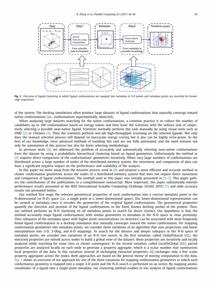
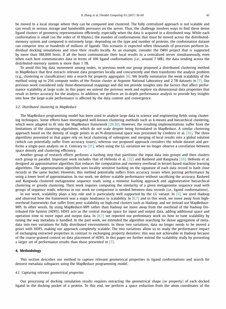
Fig. 3. From the scientific data to extracted property: From the left to right a ligand conformation in the docking pocket of a protein, the point that encodes
the geometrical property using either the 3-D or 3-Dlog mapping, and six points obtained in parallel that represent six ligand conformations clustered in
three groups with three geometries.
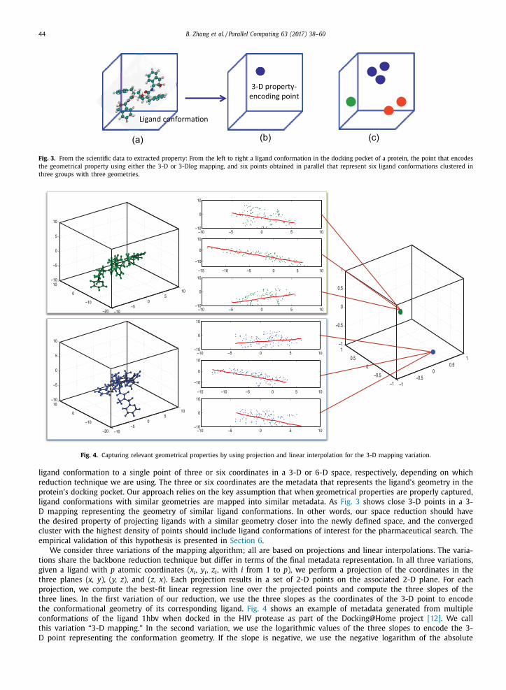
Fig. 4. Capturing relevant geometrical properties by using projection and linear interpolation for the 3-D mapping variation.
ligand conformation to a single point of three or six coordinates in a 3-D or 6-D space, respectively, depending on which
reduction technique we are using. The three or six coordinates are the metadata that represents the ligand’s geometry in the
protein’s docking pocket. Our approach relies on the key assumption that when geometrical properties are properly captured,
ligand conformations with similar geometries are mapped into similar metadata. As Fig. 3 shows close 3-D points in a 3-
D mapping representing the geometry of similar ligand conformations. In other words, our space reduction should have
the desired property of projecting ligands with a similar geometry closer into the newly defined space, and the converged
cluster with the highest density of points should include ligand conformations of interest for the pharmaceutical search. The
empirical validation of this hypothesis is presented in Section 6 .
We consider three variations of the mapping algorithm; all are based on projections and linear interpolations. The varia-
tions share the backbone reduction technique but differ in terms of the final metadata representation. In all three variations,
given a ligand with p atomic coordinates ( x i , y i , z i , with i from 1 to p ), we perform a projection of the coordinates in the
three planes ( x, y ), ( y, z ), and ( z, x ). Each projection results in a set of 2-D points on the associated 2-D plane. For each
projection, we compute the best-fit linear regression line over the projected points and compute the three slopes of the
three lines. In the first variation of our reduction, we use the three slopes as the coordinates of the 3-D point to encode
the conformational geometry of its corresponding ligand. Fig. 4 shows an example of metadata generated from multiple
conformations of the ligand 1hbv when docked in the HIV protease as part of the Docking@Home project [12] . We call
this variation “3-D mapping.” In the second variation, we use the logarithmic values of the three slopes to encode the 3-
D point representing the conformation geometry. If the slope is negative, we use the negative logarithm of the absolute
B. Zhang et al. / Parallel Computing 63 (2017) 38–60 45
value. Contrary to the 3-D mapping variation, this variation better captures the geometrical properties of conformations
that are in an almost-vertical position inside the protein pocket. In the 3-D mapping variation, when ligand conformations
are in an almost-vertical position in the protein pocket, the three resulting slopes are large. When the shape rotates or
changes slightly, the resulting slopes change significantly, possibly leading to conformations with similar shape and in an
almost-vertical position to be unmapped into a dense metadata subspace. When using the logarithmic slopes as metadata,
we decrease the changes in the metadata coordinates and thus increase the chance for ligand conformations with similar
shape to form a dense enough subspace. We call this variation “3-Dlog mapping.” In the third variation, in addition to the
slopes, we compute the intersection of the three linear regression lines with the x -axis for the line on the ( x, y ) plain, the
y -axes for the line on the ( y, z ), and the z -axis for the line on the ( z, x ). We map each conformation into a 6-D point that
coordinates the three slopes and the three line intersections. Contrary to the other two variations, this variation not only
captures the conformation shape and rotation but also stores the correct location of the ligand in the docking pocket. We
call this variation “6-D mapping.” Empirically we observed that the three slopes and the three intersections range within
well-defined ranges that represent the known, fixed docking pocket of the protein during the docking simulation generating
the data that we analyze.
The advantage of our space reduction is that it does not rely on calculations of atomic distances between two or more
ligand conformations as do most traditional analysis algorithms, such as k-means and fuzzy c-means clustering. These cal-
culations may require moving conformations across nodes, thus causing many frequent communications and multiple stor-
ages of the same data across nodes. On the contrary, our space reduction can be applied individually and concurrently
to each ligand conformation by transforming each molecule containing p atomic coordinates in the three-dimensional space
( p × 3) into a single point of (1 × 3) for the 3-D and 3-Dlog mappings and (1 × 6) for the 6-D mapping, all in the Euclidean
space. This transformation is performed locally on the compute node that generates and stores the ligand conformation, and
thus no communication is required during this phase. The projections and interpolations are low-cost processes in terms of
computing and memory requirements.
4.2. Searching for densest metadata subspaces
After mapping ligands’ geometrical properties into property-encoding metadata (i.e., three-dimensional points for the 3-
D and 3-Dlog mappings or six-dimensional points for the 6-D mapping) rather than dealing with raw atom coordinates, we
build an N-D tree by recursively partitioning the N-D space into fixed-sized subspaces, each of which form the tree nodes.
By doing so, we implicitly transform the analysis problem from a clustering or classification problem into a search of the
smaller subspaces in the newly defined metadata space (i.e., an octant for the 3-D and 3-Dlog mappings or a 6-D space for
the 6-D mapping) with high property aggregates.
From the data structure point of view, we reshape the space of property-encoding points into an N-D tree and search
for the deepest, densest tree nodes (i.e., the nodes in the deepest level of the N-D tree that contain a minimum number
of points). These nodes contain the solution to our analysis problem. Our search for dense tree nodes (or properties) be-
gins with each compute node generating its N-D tree on its own local data by recursively subdividing the space into 2 k
subspaces: 8 (2 3 ) subspaces for the 3-D and 3-Dlog mapping and 64 (2 6 ) subspaces for the 6-D mapping. Fig. 5 shows an
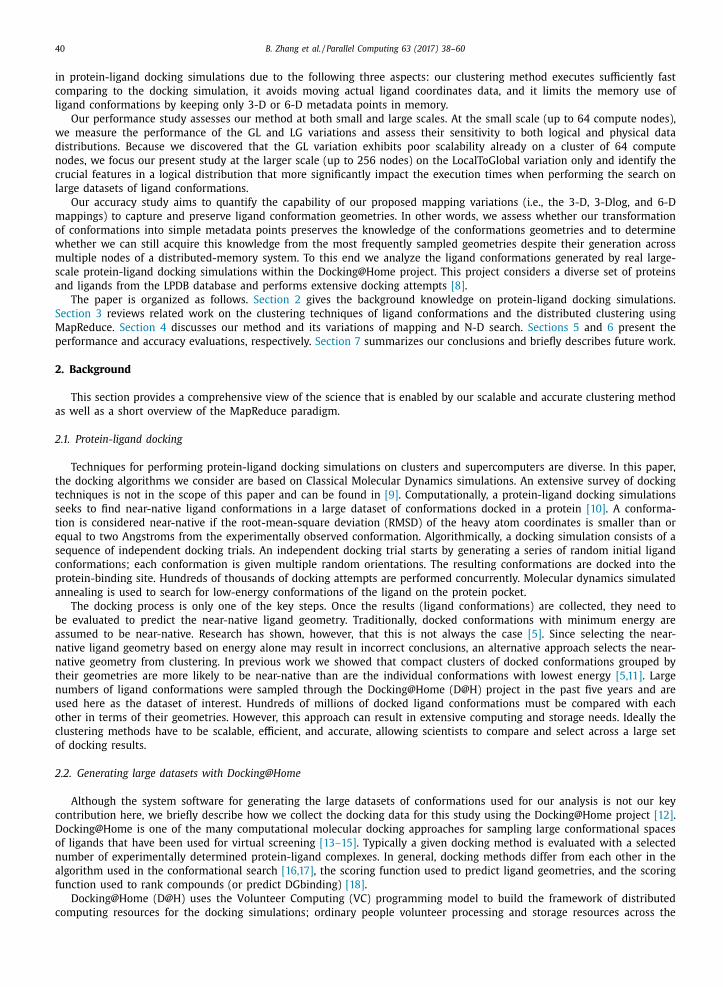
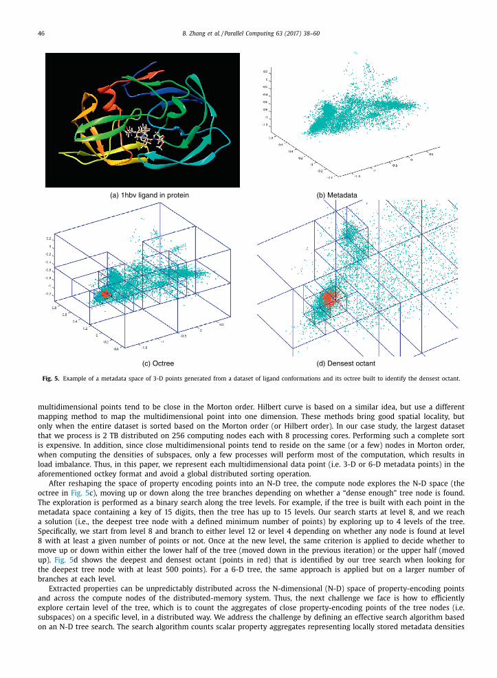
example of a dataset of 1hbv ligand conformations when docked in the HIV protease. Fig. 5 a shows the docking pocket for
the protein with a docked ligand. Fig. 5 b is the result of the 3-D mapping, after the mapping of 1 hbv ligand confirmations
into metadata has been performed. The compute nodes build an octree by assigning octkeys to the points, an N-D tree by
assigning N-D keys to the points in the case of 6-D mapping. A point belongs to a specific tree node based on its key. The
point’s key is generated as follows. We initially determine the edge size (i.e., N-D resolution) of the N-D space containing all
the projected conformations. Since we are dealing with the 3-D mapping in this example, we divide the initial space into
eight subspaces of the same size, half the original edge size. A similar process is followed for the 3-Dlog mapping; however,
when using the 6-D mapping, the metadata space is subdivided into 64 subspaces (not shown here). Every subspace is given
a unique identifier ranging from 0 to 7 for the 3-D space or from 0 to 63 for the 6-D space, based on its position in the
N-D space. The key of each point is extended by attaching the subspace identifier to the point’s key by padding the left side
with the identifier. This process is recursively repeated an arbitrary number of times on each subspace to produce a com-
plete key for each point (key [1 . . . Nkey ]) , where Nkey is the number of digits selected to represent each point. As previously
observed in [11] , Nkey can be empirically defined, and a value key of 15 digits is sufficient to capture diverse geometries in
the dataset of ligand conformations considered in this work. Fig. 5 c shows an example of the generated octree for the 3-D
mapping points in Fig. 5 b.
Alternative approaches to octkeys that can be used to map data points to octree spaces include the Z-order curve (or
Morton order) and the Hilbert curve [34,35] . Both methods map multidimensional data to one dimension. Take the Morton
order for example, the Morton code for a multidimensional point is calculated by interleaving the binary representations of
the point’s coordinate values in all dimension. For example, given a two dimensional data point < 2, 5 > , in which each
decimal value is represented by 8 bits in its binary format, we can calculate the Morton code for this data point. The binary
representation of decimal value 2 is 0 0 0 0 0 010, and the binary representation of decimal value 5 is 0 0 0 0 0101, the resulting
Morton code for < 2, 5 > is 0 0 0 0 0 0 0 0 0 010 0110, which is obtained by interleaving the binary representation of 5 and 2. This
Morton code can be used to build octrees. The general process is to compute the Morton code for every multidimensional
data point in the dataset, then sort the Morton codes. Once sorted, the Morton order ensures good spatial locality since close
46 B. Zhang et al. / Parallel Computing 63 (2017) 38–60
Fig. 5. Example of a metadata space of 3-D points generated from a dataset of ligand conformations and its octree built to identify the densest octant.
multidimensional points tend to be close in the Morton order. Hilbert curve is based on a similar idea, but use a different
mapping method to map the multidimensional point into one dimension. These methods bring good spatial locality, but
only when the entire dataset is sorted based on the Morton order (or Hilbert order). In our case study, the largest dataset
that we process is 2 TB distributed on 256 computing nodes each with 8 processing cores. Performing such a complete sort
is expensive. In addition, since close multidimensional points tend to reside on the same (or a few) nodes in Morton order,
when computing the densities of subspaces, only a few processes will perform most of the computation, which results in
load imbalance. Thus, in this paper, we represent each multidimensional data point (i.e. 3-D or 6-D metadata points) in the
aforementioned octkey format and avoid a global distributed sorting operation.
After reshaping the space of property encoding points into an N-D tree, the compute node explores the N-D space (the
octree in Fig. 5 c), moving up or down along the tree branches depending on whether a “dense enough” tree node is found.
The exploration is performed as a binary search along the tree levels. For example, if the tree is built with each point in the
metadata space containing a key of 15 digits, then the tree has up to 15 levels. Our search starts at level 8, and we reach
a solution (i.e., the deepest tree node with a defined minimum number of points) by exploring up to 4 levels of the tree.
Specifically, we start from level 8 and branch to either level 12 or level 4 depending on whether any node is found at level
8 with at least a given number of points or not. Once at the new level, the same criterion is applied to decide whether to
move up or down within either the lower half of the tree (moved down in the previous iteration) or the upper half (moved
up). Fig. 5 d shows the deepest and densest octant (points in red) that is identified by our tree search when looking for
the deepest tree node with at least 500 points). For a 6-D tree, the same approach is applied but on a larger number of
branches at each level.
Extracted properties can be unpredictably distributed across the N-dimensional (N-D) space of property-encoding points
and across the compute nodes of the distributed-memory system. Thus, the next challenge we face is how to efficiently
explore certain level of the tree, which is to count the aggregates of close property-encoding points of the tree nodes (i.e.
subspaces) on a specific level, in a distributed way. We address the challenge by defining an effective search algorithm based
on an N-D tree search. The search algorithm counts scalar property aggregates representing locally stored metadata densities
B. Zhang et al. / Parallel Computing 63 (2017) 38–60 47
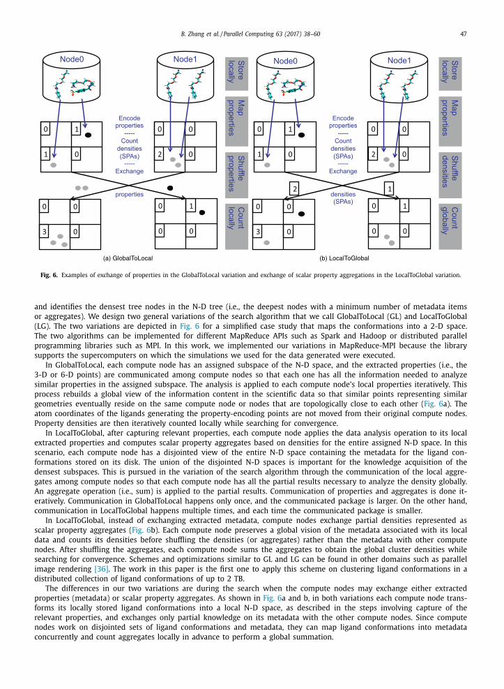
Fig. 6. Examples of exchange of properties in the GlobalToLocal variation and exchange of scalar property aggregations in the LocalToGlobal variation.
and identifies the densest tree nodes in the N-D tree (i.e., the deepest nodes with a minimum number of metadata items
or aggregates). We design two general variations of the search algorithm that we call GlobalToLocal (GL) and LocalToGlobal
(LG). The two variations are depicted in Fig. 6 for a simplified case study that maps the conformations into a 2-D space.
The two algorithms can be implemented for different MapReduce APIs such as Spark and Hadoop or distributed parallel
programming libraries such as MPI. In this work, we implemented our variations in MapReduce-MPI because the library
supports the supercomputers on which the simulations we used for the data generated were executed.
In GlobalToLocal, each compute node has an assigned subspace of the N-D space, and the extracted properties (i.e., the
3-D or 6-D points) are communicated among compute nodes so that each one has all the information needed to analyze
similar properties in the assigned subspace. The analysis is applied to each compute node’s local properties iteratively. This
process rebuilds a global view of the information content in the scientific data so that similar points representing similar
geometries eventually reside on the same compute node or nodes that are topologically close to each other ( Fig. 6 a). The
atom coordinates of the ligands generating the property-encoding points are not moved from their original compute nodes.
Property densities are then iteratively counted locally while searching for convergence.
In LocalToGlobal, after capturing relevant properties, each compute node applies the data analysis operation to its local
extracted properties and computes scalar property aggregates based on densities for the entire assigned N-D space. In this
scenario, each compute node has a disjointed view of the entire N-D space containing the metadata for the ligand con-
formations stored on its disk. The union of the disjointed N-D spaces is important for the knowledge acquisition of the
densest subspaces. This is pursued in the variation of the search algorithm through the communication of the local aggre-
gates among compute nodes so that each compute node has all the partial results necessary to analyze the density globally.
An aggregate operation (i.e., sum) is applied to the partial results. Communication of properties and aggregates is done it-
eratively. Communication in GlobalToLocal happens only once, and the communicated package is larger. On the other hand,
communication in LocalToGlobal happens multiple times, and each time the communicated package is smaller.
In LocalToGlobal, instead of exchanging extracted metadata, compute nodes exchange partial densities represented as
scalar property aggregates ( Fig. 6 b). Each compute node preserves a global vision of the metadata associated with its local
data and counts its densities before shuffling the densities (or aggregates) rather than the metadata with other compute
nodes. After shuffling the aggregates, each compute node sums the aggregates to obtain the global cluster densities while
searching for convergence. Schemes and optimizations similar to GL and LG can be found in other domains such as parallel
image rendering [36] . The work in this paper is the first one to apply this scheme on clustering ligand conformations in a
distributed collection of ligand conformations of up to 2 TB.
The differences in our two variations are during the search when the compute nodes may exchange either extracted
properties (metadata) or scalar property aggregates. As shown in Fig. 6 a and b, in both variations each compute node trans-
forms its locally stored ligand conformations into a local N-D space, as described in the steps involving capture of the
relevant properties, and exchanges only partial knowledge on its metadata with the other compute nodes. Since compute
nodes work on disjointed sets of ligand conformations and metadata, they can map ligand conformations into metadata
concurrently and count aggregates locally in advance to perform a global summation.
48 B. Zhang et al. / Parallel Computing 63 (2017) 38–60
In addition to explore the N-D tree nodes in a binary search manner along the tree levels, other alternative ways to
explore the N-D space can be to explore the tree nodes (i.e., subspaces) in a top-down or a bottom-up manner along the
tree levels. In the top-down method, we start by exploring the root tree node which contains all the property encoding
points (i.e., metadata points), proceed by moving down one level of the N-D tree, exploring the tree nodes at level one,
which are obtained by dividing the root node (entire N-D space) into 8 (in 3-D and 3-Dlog mapping) or 64 subspaces (in
6-D mapping). Then we move further down the tree by dividing each node in the upper level of the N-D tree. The process
terminates at the bottom level of the tree or when the current level of the tree does not contain a node that is dense
enough. In the bottom-up method, we start by exploring the bottom level of the tree nodes and move up one level at a
time towards the root. The process terminates at the root of the tree or when the current level of the tree does not contain
a node that is dense enough. Both methods have different requirements in communication depending on the variation used
(GL or LG). When exploring the tree nodes on a specific level of the N-D tree, we need to exchange property encoding
points and compute densities for the tree nodes at this level (in GL) or compute partial densities for the tree nodes at this
level and exchange scalar property aggregates (in LG). The communication size and pattern for each level are different. Let’s
consider the following examples, at the root level, we need to count the density of the root node (i.e., the entire N-D space).
In the GL variation, all the property encoding points are communicated to one node, and one process computes the density
of the root node. In the LG variation, all the processes computes partial density of the root node, then one scalar property
aggregate that describes the partial density of the root node is sent from every process to one process, which computes the
density of the root node. Consider the middle level of the tree, level 8 in our example, in the GL variation, all the property
encoding points with the same first 8 digits in their octkey are communicated to the same node, and the process computes
the density of this subspace (i.e., tree node). In the LG variation, each process computes the partial densities of the subspaces
starting with the same first 8 digits, and the scalar property aggregates of the subspaces are communicated to appropriate
processes for density computation. Generally, when moving down the tree, there exist more tree nodes (i.e., more subspaces)
for which we need to compute the densities. As a result, the load imbalance in communication and computation in the GL
variation and the communication size in the LG variation increase. Hence, the processing time increase, as we will further
discuss in Section 5.5 . For the same of efficiency, in our work we explore the tree levels in a binary search way. This binary
search comes with two key benefits. First, we reduce the number of tree levels that we need to explore. Second, we avoid
exploring deep levels of the tree as the bottom-up method for example does.
4.3. Integration into MapReduce-MPI
The MapReduce programming model naturally accommodates the capturing of properties from local data and the iter-
ative search for either properties or densities in its map and reduce functions, respectively. Thus, we integrated our two
variations (i.e., the GlobalToLocal and the LocalToGlobal) into the MapReduce-MPI framework rather than implementing a
new MPI-based framework from scratch.
In the GlobalToLocal variation, the operation of capturing relevant properties is implemented as the map function. It
takes the identifier and coordinates of each ligand conformation as the input key and value, respectively; applies the ge-
ometry reduction operation; and outputs the id and the property-encoding point of each conformation as the intermediate
key and value pair. The MapReduce-MPI library shuffles the property-encoding points across the distributed-memory system
to rebuild the global knowledge of the N-D space on each node. It achieves this goal by communicating all the property-
encoding points in one N-D subspace to one process such that this process has all the information needed to explore the
N-D tree locally. Then, the operation of counting property densities is implemented as the reduce function. This function
takes as input the id of the tree node and all the property-encoding points in the node and iteratively explores its lo-
cal N-D tree by counting the density of the nodes in one level of the N-D tree until the deepest and densest tree node
is found.
The LocalToGlobal variation has two map functions. The first function captures the relevant geometrical properties the
same way as in the GlobalToLocal variation. After the relevant properties are extracted by the first map function, the sec-
ond map function counts locally the property aggregates for a certain level of the N-D tree nodes. It takes the id and the
property-encoding point of each conformation as the input key and value pair, respectively; counts the aggregates for tree
nodes at a certain level; and outputs the id and aggregates of each tree node as the intermediate key and value pairs.
The exploration of the N-D tree starts at the middle level of the tree and branches up or down depending on whether a
dense enough node is found. The MapReduce-MPI framework shuffles the id and all the aggregates of each node across the
distributed-memory system. Then, the reduce function applies a sum operation to all the aggregates to compute the density
of the nodes. The process of counting aggregates (i.e., the second map function) and summing aggregates (i.e., the reduce
function) is iterated until the deepest and densest node is found.
The differences between the two variations lie in the communication phase (i.e., data shuffling). In the GlobalToLocal
variation communication happens only once, and the size of the communicated data (i.e., the property-encoding points) is
larger. In comparison, in the LocalToGlobal variation the communication happens multiple times, and each time the size of
the communicated data (i.e., local aggregates) is smaller.
B. Zhang et al. / Parallel Computing 63 (2017) 38–60 49
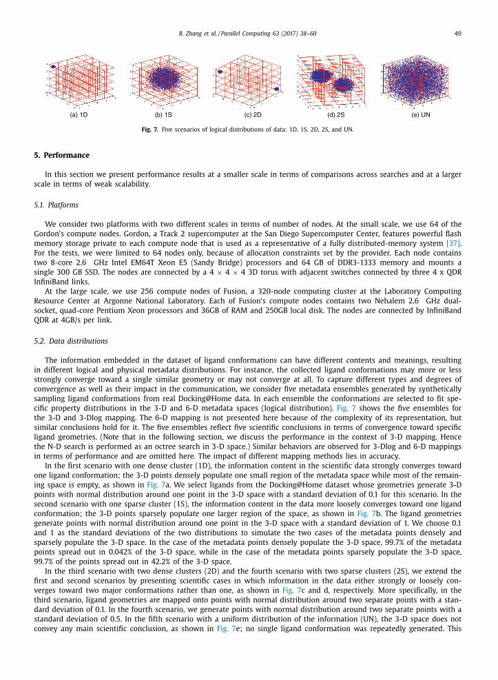
Fig. 7. Five scenarios of logical distributions of data: 1D, 1S, 2D, 2S, and UN.
5. Performance
In this section we present performance results at a smaller scale in terms of comparisons across searches and at a larger
scale in terms of weak scalability.
5.1. Platforms
We consider two platforms with two different scales in terms of number of nodes. At the small scale, we use 64 of the
Gordon’s compute nodes. Gordon, a Track 2 supercomputer at the San Diego Supercomputer Center, features powerful flash
memory storage private to each compute node that is used as a representative of a fully distributed-memory system [37] .
For the tests, we were limited to 64 nodes only, because of allocation constraints set by the provider. Each node contains
two 8-core 2.6 GHz Intel EM64T Xeon E5 (Sandy Bridge) processors and 64 GB of DDR3-1333 memory and mounts a
single 300 GB SSD. The nodes are connected by a 4 × 4 × 4 3D torus with adjacent switches connected by three 4 x QDR
InfiniBand links.
At the large scale, we use 256 compute nodes of Fusion, a 320-node computing cluster at the Laboratory Computing
Resource Center at Argonne National Laboratory. Each of Fusion’s compute nodes contains two Nehalem 2.6 GHz dual-
socket, quad-core Pentium Xeon processors and 36GB of RAM and 250GB local disk. The nodes are connected by InfiniBand
QDR at 4GB/s per link.
5.2. Data distributions
The information embedded in the dataset of ligand conformations can have different contents and meanings, resulting
in different logical and physical metadata distributions. For instance, the collected ligand conformations may more or less
strongly converge toward a single similar geometry or may not converge at all. To capture different types and degrees of
convergence as well as their impact in the communication, we consider five metadata ensembles generated by synthetically
sampling ligand conformations from real Docking@Home data. In each ensemble the conformations are selected to fit spe-
cific property distributions in the 3-D and 6-D metadata spaces (logical distribution). Fig. 7 shows the five ensembles for
the 3-D and 3-Dlog mapping. The 6-D mapping is not presented here because of the complexity of its representation, but
similar conclusions hold for it. The five ensembles reflect five scientific conclusions in terms of convergence toward specific
ligand geometries. (Note that in the following section, we discuss the performance in the context of 3-D mapping. Hence
the N-D search is performed as an octree search in 3-D space.) Similar behaviors are observed for 3-Dlog and 6-D mappings
in terms of performance and are omitted here. The impact of different mapping methods lies in accuracy.
In the first scenario with one dense cluster (1D), the information content in the scientific data strongly converges toward
one ligand conformation; the 3-D points densely populate one small region of the metadata space while most of the remain-
ing space is empty, as shown in Fig. 7 a. We select ligands from the Docking@Home dataset whose geometries generate 3-D
points with normal distribution around one point in the 3-D space with a standard deviation of 0.1 for this scenario. In the
second scenario with one sparse cluster (1S), the information content in the data more loosely converges toward one ligand
conformation; the 3-D points sparsely populate one larger region of the space, as shown in Fig. 7 b. The ligand geometries
generate points with normal distribution around one point in the 3-D space with a standard deviation of 1. We choose 0.1
and 1 as the standard deviations of the two distributions to simulate the two cases of the metadata points densely and
sparsely populate the 3-D space. In the case of the metadata points densely populate the 3-D space, 99.7% of the metadata
points spread out in 0.042% of the 3-D space, while in the case of the metadata points sparsely populate the 3-D space,
99.7% of the points spread out in 42.2% of the 3-D space.
In the third scenario with two dense clusters (2D) and the fourth scenario with two sparse clusters (2S), we extend the
first and second scenarios by presenting scientific cases in which information in the data either strongly or loosely con-
verges toward two major conformations rather than one, as shown in Fig. 7 c and d, respectively. More specifically, in the
third scenario, ligand geometries are mapped onto points with normal distribution around two separate points with a stan-
dard deviation of 0.1. In the fourth scenario, we generate points with normal distribution around two separate points with a
standard deviation of 0.5. In the fifth scenario with a uniform distribution of the information (UN), the 3-D space does not
convey any main scientific conclusion, as shown in Fig. 7 e; no single ligand conformation was repeatedly generated. This
50 B. Zhang et al. / Parallel Computing 63 (2017) 38–60
scenario can happen, for example, with insufficient sampling or inaccurate mathematical modeling of protein-ligand ener-
gies, even when using sophisticated and computationally expensive energy functions such as the Generalized Born implicit
solvent model [5,20] .
To simulate the distributed generation of ligand conformations across compute nodes, we consider three different types
of physical distributions: uniform, round-robin, and random. In uniform distributions, the ligand conformations and their
property-encoding points that belong to the same subspace in the logical distribution are located in the same physical
storage. This scenario happens most likely in a semi-decentralized distribution in which points mapping close properties are
collected by the same node or topologically close nodes; hence, there is uniformity of the property-encoding points inside
the nodes’ storages. In round-robin distributions, the conformations and their points that belong to the same subspace in
the logical distribution are stored in separate physical storage in a round-robin manner. This scenario happens most likely
in a fully decentralized, synchronous distribution in which points are collected at each predefined time interval; hence, the
data points for each time interval are stored in separate storage across the distributed system. In random distributions, the
conformations and their points are randomly stored in the physical storage of all the system nodes. This scenario simulates
the fully decentralized asynchronous manner. In each scenario, the whole dataset is roughly evenly distributed among the
physical storage sites of the testing machine.
5.3. Datasets
For testing, we build two synthetic datasets, each including the five logical distributions. We use the smaller dataset
of up to 100 million ligands (250GB) on up to 64 nodes of Gordon to compare the GlobalToLocal versus the LocalToGlobal
variations. We use the larger dataset of up to 800 million ligands (2TB) on up to 256 nodes of Fusion to study the scalability
of the LocalToGlobal variation. For the smaller dataset, we consider all three physical distributions (i.e., uniform, round-
robin, and random); for the larger dataset, we use only the round-robin distribution. In all tests we transform each ligand
conformation into a single point (metadata); the point location in the N-D tree is defined by a 15-digit key.
We compare and contrast the GlobalToLocal versus LocalToGlobal variations to assess their sensitivity to the logical and
physical distributions of the dataset. The test is performed on Gordon using the smaller dataset and up to 64 nodes available
as part of an XSEDE allocation. We measure and present the total execution time of the two variations on fifteen data dis-
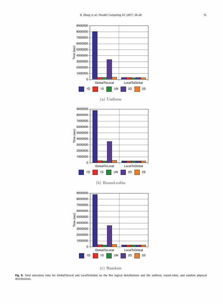
tributions (i.e., five logical distributions and three physical distributions). Fig. 8 shows the total time in seconds (aggregated
across all processes) of GlobalToLocal (GL) and LocalToGlobal (LG) for the five logical distributions (i.e., one dense cluster 1D,
one sparse cluster 1S, uniform UN, two dense clusters 2D, and two sparse clusters 2S) and the round-robin physical distri-
bution. Each time presented here is the summation of the execution times of all processes in each run. The wall time of the
program can be calculated by dividing the total execution time by the number of processes since it is a MPI programming
model. Similar results were observed in the uniform and random physical distributions. All the results are included in the
discussion below, and the complete set of times is reported in Table 1 .
When looking at the execution times across the five logical distributions for both the GlobalToLocal and LocalToGlobal
variations, we observe that for all three physical distributions, the performance of the GlobalToLocal variation is highly
sensitive to the logical distributions, while the LocalToGlobal variation delivers scalable performance across the five logical
scenarios. To be more specific, in the case of uniform physical distribution, when the information content in the dataset
strongly converges to one cluster (i.e., the 1D logical distribution), the execution time for GlobalToLocal is more than one
order of magnitude larger than when the information does not converge at all in the UN logical distribution (i.e., 8.06E03s in
1D vs. 3.35E02s in UN). When the information content in the dataset strongly converges to two clusters (i.e., the 2D logical
distribution), the execution time for GlobalToLocal is one order of magnitude larger than that of the UN logical distribution
(i.e., 3.35E03s in 2D vs. 3.35E02s in UN). For LocalToGlobal, however, the execution time varies only 3.4% across the five log-
ical distributions. Note that scenarios like the one dense cluster 1D and two dense clusters 2D are scientifically meaningful
because the information content of the science strongly converges toward a few conclusions. The GlobalToLocal variation
has significantly longer execution time for such scenarios, whereas the LocalToGlobal variation has scalable performance
regardless of the information content in the datasets.
To determine the reason for the significant variation in GlobalToLocal and the small variation in LocalToGlobal, we present
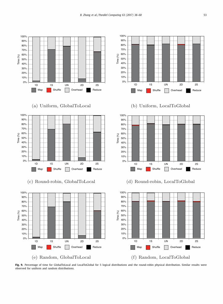
in Fig. 9 the four time components normalized with respect to the total execution time (i.e., map, shuffling, overhead, and
reduce times) across the 1,024 cores in Gordon for both variations for the five logical distributions and the three physical
distributions. The map time includes the time a process spends extracting properties during preprocessing and searching
across subspaces in the tree. The shuffling time is the time spent exchanging properties in GlobalToLocal or densities in
LocalToGlobal. The overhead time is the time introduced by the MapReduce-MPI library either for synchronizing processes at
the end of each MapReduce step (i.e., the implicit MPI_Allreduce operations to communicate small bookkeeping information
such as the total number of 〈 key, value 〉 pairs processed by the map or reduce function) or for awaiting certain processes
to complete their Map or Reduce in the case of load imbalance. The reduce time is the time to aggregate properties in
GlobalToLocal or the time to aggregate densities in LocalToGlobal. In the figure, we compute the percentages using the
average execution time in seconds over three runs; the time traces are obtained by using TAU [38] . We instrumented the
source code so that only a limited number of events (i.e., the time to perform the key map, data shuffling, and reduce
functions in the two variations) are measured by TAU; thus, the overhead introduced by TAU is negligible.
B. Zhang et al. / Parallel Computing 63 (2017) 38–60 51
Fig. 8. Total execution time for GlobalToLocal and LocalToGlobal on the five logical distributions and the uniform, round-robin, and random physical
distributions.
52 B. Zhang et al. / Parallel Computing 63 (2017) 38–60
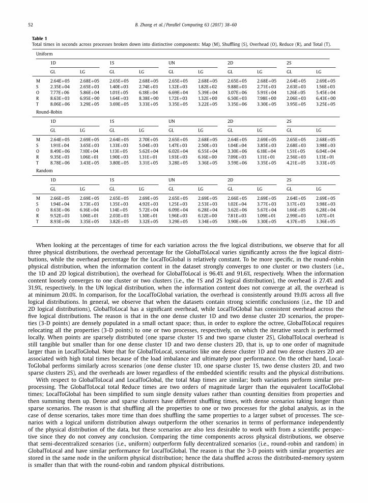
Table 1
Total times in seconds across processes broken down into distinctive components: Map (M), Shuffling (S), Overhead (O), Reduce (R), and Total (T).
Uniform
1D 1S UN 2D 2S
GL LG GL LG GL LG GL LG GL LG
M 2.64E + 05 2.68E + 05 2.65E + 05 2.68E + 05 2.65E + 05 2.68E + 05 2.65E + 05 2.68E + 05 2.64E + 05 2.69E + 05
S 2.35E + 04 2.65E + 03 1.40E + 03 2.74E + 03 1.32E + 03 1.82E + 02 9.88E + 03 2.71E + 03 2.63E + 03 1.56E + 03
O 7.77E + 06 5.86E + 04 1.01E + 05 6.18E + 04 6.69E + 04 5.39E + 04 3.07E + 06 5.91E + 04 1.26E + 05 5.45E + 04
R 8.63E + 03 6.95E + 00 1.64E + 03 8.38E + 00 1.72E + 03 1.32E + 00 6.50E + 03 7.98E + 00 2.06E + 03 6.43E + 00
T 8.06E + 06 3.29E + 05 3.69E + 05 3.33E + 05 3.35E + 05 3.22E + 05 3.35E + 06 3.30E + 05 3.95E + 05 3.25E + 05
Round-Robin
1D 1S UN 2D 2S
GL LG GL LG GL LG GL LG GL LG
M 2.64E + 05 2.69E + 05 2.64E + 05 2.70E + 05 2.65E + 05 2.68E + 05 2.64E + 05 2.69E + 05 2.65E + 05 2.68E + 05
S 1.91E + 04 3.65E + 03 1.33E + 03 5.04E + 03 1.47E + 03 2.50E + 03 1.04E + 04 3.85E + 03 2.68E + 03 3.98E + 03
O 8.49E + 06 7.10E + 04 1.13E + 05 5.62E + 04 6.02E + 04 6.55E + 04 3.30E + 06 6.18E + 04 1.51E + 05 6.04E + 04
R 9.35E + 03 1.06E + 01 1.90E + 03 1.31E + 01 1.93E + 03 6.16E + 00 7.09E + 03 1.11E + 01 2.56E + 03 1.13E + 01
T 8.78E + 06 3.43E + 05 3.80E + 05 3.31E + 05 3.28E + 05 3.36E + 05 3.59E + 06 3.35E + 05 4.21E + 05 3.33E + 05
Random
1D 1S UN 2D 2S
GL LG GL LG GL LG GL LG GL LG
M 2.66E + 05 2.69E + 05 2.65E + 05 2.69E + 05 2.65E + 05 2.69E + 05 2.66E + 05 2.69E + 05 2.64E + 05 2.69E + 05
S 1.94E + 04 3.73E + 03 1.35E + 03 4.92E + 03 1.25E + 03 2.53E + 03 1.02E + 04 3.77E + 03 3.17E + 03 3.98E + 03
O 8.63E + 06 6.16E + 04 1.14E + 05 5.72E + 04 6.09E + 04 6.28E + 04 3.62E + 06 5.67E + 04 1.66E + 05 6.28E + 04
R 9.52E + 03 1.06E + 01 2.03E + 03 1.30E + 01 1.96E + 03 6.12E + 00 7.81E + 03 1.09E + 01 2.99E + 03 1.07E + 01
T 8.93E + 06 3.35E + 05 3.82E + 05 3.32E + 05 3.29E + 05 3.34E + 05 3.90E + 06 3.30E + 05 4.37E + 05 3.36E + 05
When looking at the percentages of time for each variation across the five logical distributions, we observe that for all
three physical distributions, the overhead percentage for the GlobalToLocal varies significantly across the five logical distri-
butions, while the overhead percentage for the LocalToGlobal is relatively constant. To be more specific, in the round-robin
physical distribution, when the information content in the dataset strongly converges to one cluster or two clusters (i.e.,
the 1D and 2D logical distribution), the overhead for GlobalToLocal is 96.4% and 91.6%, respectively. When the information
content loosely converges to one cluster or two clusters (i.e., the 1S and 2S logical distribution), the overhead is 27.4% and
31.9%, respectively. In the UN logical distribution, when the information content does not converge at all, the overhead is
at minimum 20.0%. In comparison, for the LocalToGlobal variation, the overhead is consistently around 19.0% across all five
logical distributions. In general, we observe that when the datasets contain strong scientific conclusions (i.e., the 1D and
2D logical distributions), GlobalToLocal has a significant overhead, while LocalToGlobal has consistent overhead across the
five logical distributions. The reason is that in the one dense cluster 1D and two dense cluster 2D scenarios, the proper-
ties (3-D points) are densely populated in a small octant space; thus, in order to explore the octree, GlobalToLocal requires
relocating all the properties (3-D points) to one or two processes, respectively, on which the iterative search is performed
locally. When points are sparsely distributed (one sparse cluster 1S and two sparse cluster 2S), GlobalToLocal overhead is
still tangible but smaller than for one dense cluster 1D and two dense clusters 2D, that is, up to one order of magnitude
larger than in LocalToGlobal. Note that for GlobalToLocal, scenarios like one dense cluster 1D and two dense clusters 2D are
associated with high total times because of the load imbalance and ultimately poor performance. On the other hand, Local-
ToGlobal performs similarly across scenarios (one dense cluster 1D, one sparse cluster 1S, two dense clusters 2D, and two
sparse clusters 2S), and the overheads are lower regardless of the embedded scientific results and the physical distributions.
With respect to GlobalToLocal and LocalToGlobal, the total Map times are similar; both variations perform similar pre-
processing. The GlobalToLocal total Reduce times are two orders of magnitude larger than the equivalent LocalToGlobal
times; LocalToGlobal has been simplified to sum single density values rather than counting densities from properties and
then summing them up. Dense and sparse clusters have different shuffling times, with dense scenarios taking longer than
sparse scenarios. The reason is that shuffling all the properties to one or two processes for the global analysis, as in the
case of dense scenarios, takes more time than does shuffling the same properties to a larger subset of processes. The sce-
narios with a logical uniform distribution always outperform the other scenarios in terms of performance independently
of the physical distribution of the data, but these scenarios are also less desirable to work with from a scientific perspec-
tive since they do not convey any conclusion. Comparing the time components across physical distributions, we observe
that semi-decentralized scenarios (i.e., uniform) outperform fully decentralized scenarios (i.e., round-robin and random) in
GlobalToLocal and have similar performance for LocalToGlobal. The reason is that the 3-D points with similar properties are
stored in the same node in the uniform physical distribution; hence the data shuffled across the distributed-memory system
is smaller than that with the round-robin and random physical distributions.
B. Zhang et al. / Parallel Computing 63 (2017) 38–60 53
Fig. 9. Percentage of time for GlobalToLocal and LocalToGlobal for 5 logical distributions and the round-robin physical distribution. Similar results were
observed for uniform and random distributions.
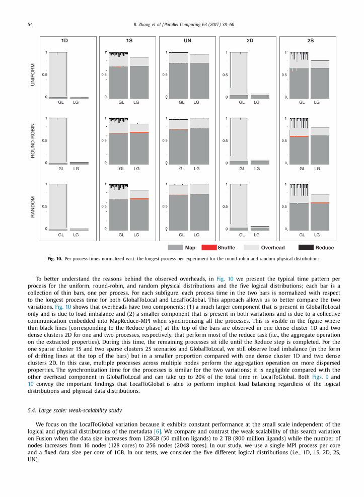
54 B. Zhang et al. / Parallel Computing 63 (2017) 38–60
Fig. 10. Per process times normalized w.r.t. the longest process per experiment for the round-robin and random physical distributions.
To better understand the reasons behind the observed overheads, in Fig. 10 we present the typical time pattern per
process for the uniform, round-robin, and random physical distributions and the five logical distributions; each bar is a
collection of thin bars, one per process. For each subfigure, each process time in the two bars is normalized with respect
to the longest process time for both GlobalToLocal and LocalToGlobal. This approach allows us to better compare the two
variations. Fig. 10 shows that overheads have two components: (1) a much larger component that is present in GlobalToLocal
only and is due to load imbalance and (2) a smaller component that is present in both variations and is due to a collective
communication embedded into MapReduce-MPI when synchronizing all the processes. This is visible in the figure where
thin black lines (corresponding to the Reduce phase) at the top of the bars are observed in one dense cluster 1D and two
dense clusters 2D for one and two processes, respectively, that perform most of the reduce task (i.e., the aggregate operation
on the extracted properties). During this time, the remaining processes sit idle until the Reduce step is completed. For the
one sparse cluster 1S and two sparse clusters 2S scenarios and GlobalToLocal, we still observe load imbalance (in the form
of drifting lines at the top of the bars) but in a smaller proportion compared with one dense cluster 1D and two dense
clusters 2D. In this case, multiple processes across multiple nodes perform the aggregation operation on more dispersed
properties. The synchronization time for the processes is similar for the two variations; it is negligible compared with the
other overhead component in GlobalToLocal and can take up to 20% of the total time in LocalToGlobal. Both Figs. 9 and
10 convey the important findings that LocalToGlobal is able to perform implicit load balancing regardless of the logical
distributions and physical data distributions.
5.4. Large scale: weak-scalability study
We focus on the LocalToGlobal variation because it exhibits constant performance at the small scale independent of the
logical and physical distributions of the metadata [6] . We compare and contrast the weak scalability of this search variation
on Fusion when the data size increases from 128GB (50 million ligands) to 2 TB (800 million ligands) while the number of
nodes increases from 16 nodes (128 cores) to 256 nodes (2048 cores). In our study, we use a single MPI process per core
and a fixed data size per core of 1GB. In our tests, we consider the five different logical distributions (i.e., 1D, 1S, 2D, 2S,
UN).
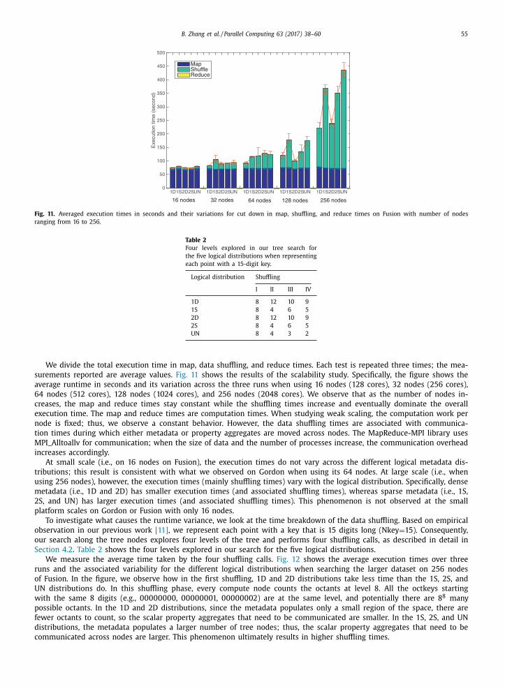
B. Zhang et al. / Parallel Computing 63 (2017) 38–60 55
Fig. 11. Averaged execution times in seconds and their variations for cut down in map, shuffling, and reduce times on Fusion with number of nodes
ranging from 16 to 256.
Table 2
Four levels explored in our tree search for
the five logical distributions when representing
each point with a 15-digit key.
Logical distribution Shuffling
I II III IV
1D 8 12 10 9
1S 8 4 6 5
2D 8 12 10 9
2S 8 4 6 5
UN 8 4 3 2
We divide the total execution time in map, data shuffling, and reduce times. Each test is repeated three times; the mea-
surements reported are average values. Fig. 11 shows the results of the scalability study. Specifically, the figure shows the
average runtime in seconds and its variation across the three runs when using 16 nodes (128 cores), 32 nodes (256 cores),
64 nodes (512 cores), 128 nodes (1024 cores), and 256 nodes (2048 cores). We observe that as the number of nodes in-
creases, the map and reduce times stay constant while the shuffling times increase and eventually dominate the overall
execution time. The map and reduce times are computation times. When studying weak scaling, the computation work per
node is fixed; thus, we observe a constant behavior. However, the data shuffling times are associated with communica-
tion times during which either metadata or property aggregates are moved across nodes. The MapReduce-MPI library uses
MPI_Alltoallv for communication; when the size of data and the number of processes increase, the communication overhead
increases accordingly.
At small scale (i.e., on 16 nodes on Fusion), the execution times do not vary across the different logical metadata dis-
tributions; this result is consistent with what we observed on Gordon when using its 64 nodes. At large scale (i.e., when
using 256 nodes), however, the execution times (mainly shuffling times) vary with the logical distribution. Specifically, dense
metadata (i.e., 1D and 2D) has smaller execution times (and associated shuffling times), whereas sparse metadata (i.e., 1S,
2S, and UN) has larger execution times (and associated shuffling times). This phenomenon is not observed at the small
platform scales on Gordon or Fusion with only 16 nodes.
To investigate what causes the runtime variance, we look at the time breakdown of the data shuffling. Based on empirical
observation in our previous work [11] , we represent each point with a key that is 15 digits long (Nkey = 15). Consequently,
our search along the tree nodes explores four levels of the tree and performs four shuffling calls, as described in detail in
Section 4.2 . Table 2 shows the four levels explored in our search for the five logical distributions.
We measure the average time taken by the four shuffling calls. Fig. 12 shows the average execution times over three
runs and the associated variability for the different logical distributions when searching the larger dataset on 256 nodes
of Fusion. In the figure, we observe how in the first shuffling, 1D and 2D distributions take less time than the 1S, 2S, and
UN distributions do. In this shuffling phase, every compute node counts the octants at level 8. All the octkeys starting
with the same 8 digits (e.g., 0 0 0 0 0 0 0 0, 0 0 0 0 0 0 01, 0 0 0 0 0 0 02) are at the same level, and potentially there are 8 8 many
possible octants. In the 1D and 2D distributions, since the metadata populates only a small region of the space, there are
fewer octants to count, so the scalar property aggregates that need to be communicated are smaller. In the 1S, 2S, and UN
distributions, the metadata populates a larger number of tree nodes; thus, the scalar property aggregates that need to be
communicated across nodes are larger. This phenomenon ultimately results in higher shuffling times.
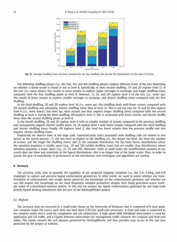
56 B. Zhang et al. / Parallel Computing 63 (2017) 38–60
Fig. 12. Averaged shuffling times and their variations for the four shuffling calls and the five distributions on 256 nodes of Fusion.
The following shuffling phases (i.e., the 2nd, 3rd, and 4th shuffling phases) explore different levels of the tree depending
on whether a dense octant is found or not at level 8. Specifically, in their second shuffling, 1D and 2D explore level 12 of
the tree (i.e., move down); this results in more octants to explore, larger messages to exchange, and longer shuffling times
compared with the first shuffling phase at level 8. However, 1S, 2S, and UN explore level 4 of the tree (i.e., move up);
this results in fewer octants to explore, smaller messages to exchange, and shorter shuffling times compared with the first
shuffling.
In the third shuffling, 1D and 2D explore level 10 (i.e., move up); this shuffling deals with fewer octants compared with
the second shuffling and, ultimately, shorter shuffling times than at level 12. This is not the case for 1S and 2S that explore
level 6 (i.e., move down); this level has more octants and thus requires longer shuffling times compared with the second
shuffling at level 4. During the third shuffling, UN explores level 3; this is associated with fewer octants and shorter shuffle
times than the second shuffling phase at level 4.
In the fourth shuffling, 1D and 2D explore level 9 with its smaller number of octants compared to the previous shuffling
and consequently requires shorter shuffle times. 1S, 2S explore level 5 with fewer octants compared with the third shuffling
and shorter shuffling times. Finally, UN explores level 2; this level has fewer octants than the previous shuffle and also
requires shorter shuffling times.
Empirically we observe how, at the large scale, communication times associated with shuffling calls are related to two
factors in the search process: (1) the tree level to explore in the shuffling (i.e., the deeper the level, the more the number
of octants, and the longer the shuffling times) and (2) the metadata distribution. For the latter factor, distributions where
the metadata populates a smaller space (e.g., 1D and 2D) exhibit shuffling times that are smaller than distributions where
metadata populates a larger space (e.g., 1S, 2S, and UN). Moreover, while at small scales the LocalToGlobal variation of our
search does not show any sensitivity to the logical distributions, this is no longer true at the larger scales. Thus, in order to
pursue the goal of insensitivity of performance to the distribution, new techniques and algorithms are needed.
6. Accuracy
The accuracy study aims to quantify the capability of our proposed mapping variations (i.e., the 3-D, 3-Dlog, and 6-D
mappings) to capture and preserve ligand conformation geometries. In other words, we want to assess whether our trans-
formation of conformations into simple points preserves the knowledge on the conformations geometry and whether we
can still acquire this knowledge on the most frequently sampled geometries despite their being generated across multi-
ple nodes of a distributed-memory system. To this end we analyze the ligand conformations generated by real large-scale
protein-ligand docking simulations that are part of the Docking@Home project.
6.1. Platform
The accuracy tests are executed in a small-scale cluster at the University of Delaware that is composed of 8 dual quad-
core compute nodes (64 cores), each with two Intel Xeon 2.50 GHz quad-core processors. A front-end node is connected to
the compute nodes and is used for compilation and job submissions. A high-speed DDR InfiniBand interconnect is used for
application and I/O traffic, and a Gigabit Ethernet interconnect for management traffic connects the compute and front-end
nodes. The cluster mounts the real datasets generated by Docking@Home and thus provides easy access to the real data
generated by the project at runtime.
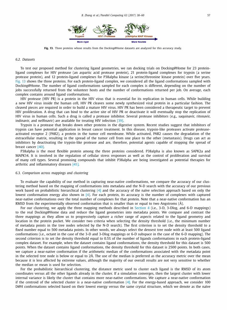
B. Zhang et al. / Parallel Computing 63 (2017) 38–60 57
Fig. 13. Three proteins whose results from the Docking@Home datasets are analyzed for this accuracy study.
6.2. Datasets
To test our proposed method for clustering ligand geometries, we ran docking trials on Docking@Home for 23 protein-
ligand complexes for HIV protease (an aspartic acid protease protein), 21 protein-ligand complexes for trypsin (a serine
protease protein), and 12 protein-ligand complexes for P38alpha kinase (a serine/threonine kinase protein) over five years.
Fig. 13 shows the three proteins. For each protein-ligand complex, we considered all the ligand conformations sampled with
Docking@Home. The number of ligand conformations sampled for each complex is different, depending on the number of
jobs successfully returned from the volunteer hosts and the number of conformations returned per job. On average, each
complex contains around ligand conformations.
HIV protease (HIV PR) is a protein in the HIV virus that is essential for its replication in human cells. While building
a new HIV virus inside the human cell, HIV PR cleaves some newly synthesized viral protein in a particular fashion. The
cleaved pieces are required in order to build a mature HIV virus. HIV PR has been considered a therapeutic target to prevent
HIV proliferation. A drug that can bind to the active site of HIV PR or deactivate it will eventually stop the replication of
HIV virus in human cells. Such a drug is called a protease inhibitor. Several protease inhibitors (e.g., saquinavir, ritonavir,
indinavir, and nelfinavir) are available for treating HIV infection [39] .
Trypsin is a protease that breaks down other proteins in the digestive system. Recent studies suggest that inhibitors of
trypsin can have potential application in breast cancer treatment. In this disease, trypsin-like proteases activate protease-
activated receptor 2 (PAR2), a protein in the tumor cell membrane. While activated, PAR2 causes the degradation of the
extracellular matrix, resulting in the spread of the tumor cell from one place to the other (metastasis). Drugs can act as
inhibitors by deactivating the trypsin-like protease and are, therefore, potential agents capable of stopping the spread of
breast cancer [40] .
P38alpha is the most flexible protein among the three proteins considered. P38alpha is also known as SAPK2a and
MAPK14. It is involved in the regulation of cellular stress responses as well as the control of proliferation and survival
of many cell types. Several promising compounds that inhibit P38alpha are being investigated as potential therapies for
arthritic and inflammatory diseases [41] .
6.3. Comparison across mappings and clustering
To evaluate the capability of our method in capturing near-native conformations, we compare the accuracy of our clus-
tering method based on the mapping of conformations into metadata and the N-D search with the accuracy of our previous
work based on probabilistic hierarchical clustering [4] and the accuracy of the naïve selection approach based on only the
lowest conformation energy also shown in [4] . For each protein, its accuracy is the number of complexes with captured
near-native conformations over the total number of complexes for that protein. Note that a near-native conformation has an
RMSD from the experimentally observed conformation that is smaller than or equal to two Angstroms ( ̊A).
For our clustering, we apply the three mapping methods described in Section 4 (i.e., 3-D, 3-Dlog, and 6-D mappings)
to the real Docking@Home data and reduce the ligand geometries into metadata points. We compare and contrast the
three mappings as they allow us to progressively capture a richer range of aspects related to the ligand geometry and
location in the protein pocket. We consider two criteria when selecting the density threshold (i.e., the minimum number
of metadata points in the tree nodes selected by the N-D search). The first criterion is to set the density threshold to a
fixed number equal to 500 metadata points. In other words, we always select the densest tree node with at least 500 ligand
conformations (i.e., octant in the case of the 3-D and 3-Dlog mappings or 6-D subspace in the case of the 6-D mapping). The
second criterion is to set the density threshold equal to 0.5% of the number of ligands conformations in each protein-ligand
complex dataset. For example, when the dataset contains ligand conformations, the density threshold for this dataset is 500
points. When the dataset contains ligand conformations, the density threshold for this dataset is 2500 points. In both cases,
we capture a near-native conformation if the arithmetic median of the conformations associated with the metadata point
in the selected tree node is below or equal to 2 ̊A. The use of the median is preferred as the accuracy metric over the mean
because it is less affected by extreme values, although the majority of our overall results are not very sensitive to whether
the median or mean is used for selection.
For the probabilistic hierarchical clustering, the distance metric used to cluster each ligand is the RMSD of its atom
coordinates versus all the other ligands already in the cluster. If a simulation converges, then the largest cluster with lower
internal variance is likely the cluster that contains more near-native conformations. We capture a near-native conformation
if the centroid of the selected cluster is a near-native conformation [4] . For the energy-based approach, we consider 100
D@H conformations selected based on their lowest energy versus the same crystal structure, which we denote as the naïve
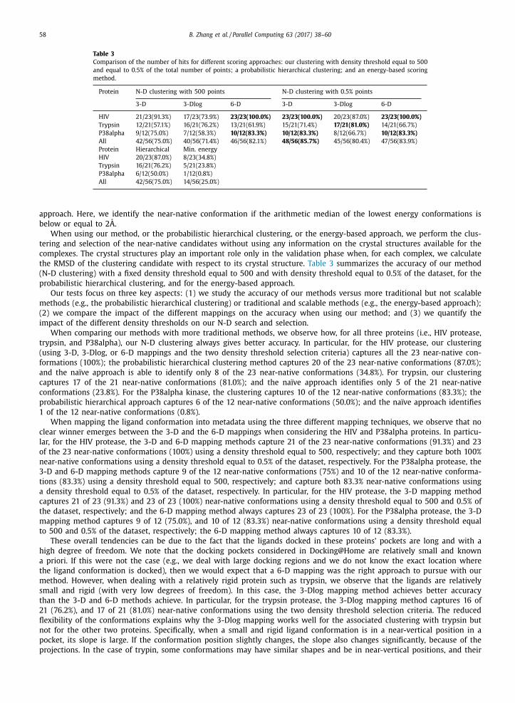
58 B. Zhang et al. / Parallel Computing 63 (2017) 38–60
Table 3
Comparison of the number of hits for different scoring approaches: our clustering with density threshold equal to 500
and equal to 0.5% of the total number of points; a probabilistic hierarchical clustering; and an energy-based scoring
method.
Protein N-D clustering with 500 points N-D clustering with 0.5% points
3-D 3-Dlog 6-D 3-D 3-Dlog 6-D
HIV 21/23(91.3%) 17/23(73.9%) 23/23(100.0%) 23/23(100.0%) 20/23(87.0%) 23/23(100.0%)
Trypsin 12/21(57.1%) 16/21(76.2%) 13/21(61.9%) 15/21(71.4%) 17/21(81.0%) 14/21(66.7%)
P38alpha 9/12(75.0%) 7/12(58.3%) 10/12(83.3%) 10/12(83.3%) 8/12(66.7%) 10/12(83.3%)
All 42/56(75.0%) 40/56(71.4%) 46/56(82.1%) 48/56(85.7%) 45/56(80.4%) 47/56(83.9%)
Protein Hierarchical Min. energy
HIV 20/23(87.0%) 8/23(34.8%)
Trypsin 16/21(76.2%) 5/21(23.8%)
P38alpha 6/12(50.0%) 1/12(0.8%)
All 42/56(75.0%) 14/56(25.0%)
approach. Here, we identify the near-native conformation if the arithmetic median of the lowest energy conformations is
below or equal to 2 ̊A.
When using our method, or the probabilistic hierarchical clustering, or the energy-based approach, we perform the clus-
tering and selection of the near-native candidates without using any information on the crystal structures available for the
complexes. The crystal structures play an important role only in the validation phase when, for each complex, we calculate
the RMSD of the clustering candidate with respect to its crystal structure. Table 3 summarizes the accuracy of our method
(N-D clustering) with a fixed density threshold equal to 500 and with density threshold equal to 0.5% of the dataset, for the
probabilistic hierarchical clustering, and for the energy-based approach.
Our tests focus on three key aspects: (1) we study the accuracy of our methods versus more traditional but not scalable
methods (e.g., the probabilistic hierarchical clustering) or traditional and scalable methods (e.g., the energy-based approach);
(2) we compare the impact of the different mappings on the accuracy when using our method; and (3) we quantify the
impact of the different density thresholds on our N-D search and selection.
When comparing our methods with more traditional methods, we observe how, for all three proteins (i.e., HIV protease,
trypsin, and P38alpha), our N-D clustering always gives better accuracy. In particular, for the HIV protease, our clustering
(using 3-D, 3-Dlog, or 6-D mappings and the two density threshold selection criteria) captures all the 23 near-native con-
formations (100%); the probabilistic hierarchical clustering method captures 20 of the 23 near-native conformations (87.0%);
and the naïve approach is able to identify only 8 of the 23 near-native conformations (34.8%). For trypsin, our clustering
captures 17 of the 21 near-native conformations (81.0%); and the naïve approach identifies only 5 of the 21 near-native
conformations (23.8%). For the P38alpha kinase, the clustering captures 10 of the 12 near-native conformations (83.3%); the
probabilistic hierarchical approach captures 6 of the 12 near-native conformations (50.0%); and the naïve approach identifies
1 of the 12 near-native conformations (0.8%).
When mapping the ligand conformation into metadata using the three different mapping techniques, we observe that no
clear winner emerges between the 3-D and the 6-D mappings when considering the HIV and P38alpha proteins. In particu-
lar, for the HIV protease, the 3-D and 6-D mapping methods capture 21 of the 23 near-native conformations (91.3%) and 23
of the 23 near-native conformations (100%) using a density threshold equal to 500, respectively; and they capture both 100%
near-native conformations using a density threshold equal to 0.5% of the dataset, respectively. For the P38alpha protease, the
3-D and 6-D mapping methods capture 9 of the 12 near-native conformations (75%) and 10 of the 12 near-native conforma-
tions (83.3%) using a density threshold equal to 500, respectively; and capture both 83.3% near-native conformations using
a density threshold equal to 0.5% of the dataset, respectively. In particular, for the HIV protease, the 3-D mapping method
captures 21 of 23 (91.3%) and 23 of 23 (100%) near-native conformations using a density threshold equal to 500 and 0.5% of
the dataset, respectively; and the 6-D mapping method always captures 23 of 23 (100%). For the P38alpha protease, the 3-D
mapping method captures 9 of 12 (75.0%), and 10 of 12 (83.3%) near-native conformations using a density threshold equal
to 500 and 0.5% of the dataset, respectively; the 6-D mapping method always captures 10 of 12 (83.3%).
These overall tendencies can be due to the fact that the ligands docked in these proteins’ pockets are long and with a
high degree of freedom. We note that the docking pockets considered in Docking@Home are relatively small and known
a priori. If this were not the case (e.g., we deal with large docking regions and we do not know the exact location where
the ligand conformation is docked), then we would expect that a 6-D mapping was the right approach to pursue with our
method. However, when dealing with a relatively rigid protein such as trypsin, we observe that the ligands are relatively
small and rigid (with very low degrees of freedom). In this case, the 3-Dlog mapping method achieves better accuracy
than the 3-D and 6-D methods achieve. In particular, for the trypsin protease, the 3-Dlog mapping method captures 16 of
21 (76.2%), and 17 of 21 (81.0%) near-native conformations using the two density threshold selection criteria. The reduced
flexibility of the conformations explains why the 3-Dlog mapping works well for the associated clustering with trypsin but
not for the other two proteins. Specifically, when a small and rigid ligand conformation is in a near-vertical position in a
pocket, its slope is large. If the conformation position slightly changes, the slope also changes significantly, because of the
projections. In the case of trypin, some conformations may have similar shapes and be in near-vertical positions, and their
B. Zhang et al. / Parallel Computing 63 (2017) 38–60 59
slopes may differ to the extent such that the mapping may not result in a dense enough subspace containing the metadata.
By taking the log of the slopes, we slow the slope differences when dealing with vertical ligand conformations.
When dealing with different selection criteria (i.e., 500 points or a variable density threshold equal to 0.5%), we observe
how using a variable density threshold achieves better accuracy than using a fixed threshold equal to 500 for each indi-
vidual dataset. Moreover, when a fixed density threshold equal to 500 is used, our method always outperforms the naïve
approach for all the complexes; and our method also outperforms (for HIV and P38alpha) or is as accurate as (for trypsin)
the probabilistic hierarchical clustering. Additionally, when a variable density threshold equal to 0.5% of the number of lig-
and conformations in the protein-ligand complex dataset is used, our N-D clustering always outperforms both the naïve
approach and the probabilistic hierarchical clustering. In particular, for the HIV protease, when using a variable density,
the 3-D, 3-Dlog, and 6-D achieve 100%, 87.0%, and 100% accuracy, respectively; when using a fixed threshold, the 3-D, 3-
Dlog, and 6-D achieve 91.3%, 73.9%, and 100% accuracy, respectively. Similar results are observed for trypsin and P38alpha
protease.
The 3-Dlog mapping method captures 16 of 21 (76.2%), and 17 of 21 (81.0%) near-native conformations using the two
density threshold selection criteria. To be more specific, for the HIV protease, the N-D clustering captures all the near-native
conformations (100.0%), 20 of 23 (87.0%), and 23 of 23 (100.0%) using the 3-D, 3-Dlog, and 6-D mappings, respectively. For
trypsin, the N-D clustering captures 15 of the 21 near-native conformations (71.4%), 17 of 21 (81.0%), and 14 of 21 (66.7%)
using 3-D, 3-Dlog, and 6-D, respectively. For the P38alpha kinase, our N-D clustering captures 10 of the 12 near-native
conformations (83.3%), 8 of 12 (66.7%), and 10 of 12 (83.3%) using 3-D, 3-Dlog, and 6-D, respectively. Overall, we observe
how a variable density threshold better captures the convergence of docking simulations to a single ligand conformation
that also matches crystal structure findings.
7. Conclusion and future work
This paper focuses on avoiding data movement when analyzing scientific datasets comprising many complex data records
distributed across nodes of a large distributed-memory system. We present a general method for data analysis – namely,
clustering or classification – and apply it to structural biology datasets. The method performs a local, single preprocessing
of the data to extract relevant properties (i.e., the geometrical properties including the shape and position) of a ligand
conformation in a large dataset of millions of confirmations. We discuss variations of the general method including three
ways to perform data reduction of the ligand conformations to metadata and two ways to perform the metadata space
search.
We evaluate the performance of our method on 64 nodes of Gordon at the San Diego Supercomputer Center and 256
nodes of Fusion at Argonne National Laboratory, considering fifteen scenarios by combining five clustering configurations
and three physical distributions of the data. At small scale on 64 nodes of Gordon, out method shows that when exchanging
smaller messages of scalar property aggregates in the LocalToGlobal variation, the execution time is not sensitive to metadata
distributions in the datasets: it varies only 3.4% across the five logical distributions. The GlobalToLocal variation, on the other
hand, is sensitive to the metadata distributions. At large scale on 256 nodes of Fusion, our method shows that the data-
shuffling stage dominates the execution time, and the shuffling time is affected by the metadata distribution as well as the
level of trees explored in the N-dimensional tree. Moreover, we evaluate the accuracy of our method using three mapping
methods and two density threshold selection criteria. The results on 56 ligands of three proteins show that our method
can achieve 100%, 81.0%, and 85.7% clustering accuracy on protein HIV, trypsin, and P38alpha, respectively, whereas the
traditional hierarchical-based clustering achieves only 87.0%, 76.2%, and 50.0% accuracy, respectively. Our accuracy analysis
also reveals important insights into the fact that the 3-D and 6-D mapping methods work better on larger flexible ligands,
whereas the 3-Dlog mapping method works better on smaller, more rigid ligands.
Our variations are applicable to diverse scientific datasets and other distributed frameworks beyond the one considered
in this paper and can result in scientific analyses that are not sensitive to data content and distribution. In the future, we
plan to investigate and improve the scalability of our method at large scale by improving the performance of the shuffling
stage of the MapReduce-MPI library. Moreover, we plan to extend our metadata mapping method by using the angles of
the three linear regression lines in the 2-D space that are in a fixed range of 0 and 2 π and to apply our method in virtual
screening.
Acknowledgments
This work was supported in part by NSF grant CCF1318445 and by the U.S. Department of Energy , Office of Science, under
contract DE-AC02-06CH11357 . This research used the Argonne Laboratory Computing Research Center “Fusion” cluster.
We thank Dr. Roger S. Armen (Thomas Jefferson University) and the Docking@Home volunteers for providing us with
essential resources for our protein-ligand docking simulations. The code of our clustering and sample ligands input data are
available on github: https://github.com/TauferLab .
References
[1] M. Taufer , R.S. Armen , J. Chen , P.J. Teller , C.L. Brooks III , Computational multi-scale modeling in protein-ligand docking, IEEE Eng. Med. Biol. Mag. 28(2) (2009) 58–69 .
60 B. Zhang et al. / Parallel Computing 63 (2017) 38–60
[2] W. Humphrey , A. Dalke , K. Schulten , VMD – visual molecular dynamics, J. Mol. Graph. 14 (1996) 33–38 . [3] S. Ceri , R. Manthey , Chimera: a model and language for active DOOD systems, in: Proceedings of the 2nd East-West Database Workshop, Workshops
in Computing, Springer, 1994, pp. 3–16 . [4] T. Estrada , R.S. Armen , M. Taufer , Automatic selection of near-native protein-ligand conformations using a hierarchical clustering and volunteer com-
puting, in: Proceedings of the First ACM International Conference on Bioinformatics and Computational Biology, 2010, pp. 204–213 . [5] T. Estrada , B. Zhang , P. Cicotti , R.S. Armen , M. Taufer , Accurate analysis of large datasets of protein-ligand binding geometries using advanced clustering
methods, Comput. Biol. Med. 42 (7) (2012) .
[6] B. Zhang , T. Estarda , P. Cicotti , M. Taufer , On efficiently capturing scientific properties in distributed big data without moving the data - a case studyin distributed structural biology using MapReduce, in: Proceedings of the 2013 IEEE 16th International Conference on Computational Science and
Engineering, 2013, pp. 817–822 . [7] B. Zhang , T. Estrada , P. Cicotti , P. Balaji , M. Taufer , Accurate scoring of drug conformations at the extreme scale, in: Proceedings of the IEEE International
Scalable Computing Challenges (SCALE 2015) - co-located with the 15th IEEE/ACM International Symposium on Cluster, Cloud and Grid Computing,2015, pp. 817–822 .
[8] O. Roche , R. Kiyama , C.L.B. III , Ligand-protein database: linking protein-ligand complex structures to binding data, J. Med. Chem. 44 (22) (2001)3592–3598 .
[9] R. Armen , E. May , M. Taufer , Protein Docking, Springer, 2011 .
[10] A. Jain , Bias, reporting, and sharing: computational evaluations of docking methods, J. Comput. Aided Mol. Des. 22 (3–4) (2008) 201–212 . [11] T. Estrada , B. Zhang , P. Cicotti , R.S. Armen , M. Taufer , Reengineering high-throughput molecular datasets for scalable clustering using MapReduce, in:
Proceedings of the 14th IEEE International Conference on High Performance Computing and Communications, 2012, pp. 351–359 . [12] M. Taufer , R.S. Armen , J. Chen , P.J. Teller , C.L. Brooks , Computational multiscale modeling in protein-ligand docking, IEEE Eng. Med. Biol. Mag. 28 (2)
(2009) 58–69 . [13] M. Rarey , B. Kramer , T. Lengauer , G.A. Klebe , A fast flexible docking method using an incremental construction algorithm, J. Mol. Biol. 261 (3) (1996)
470–489 .
[14] R. Abagyan , M. Totrov , D. Kuznetsov , A new method for protein modeling and design: applications to docking and structure prediction from thedistorted native conformation, J. Comput. Chem. 15 (5) (1994) 488–506 .
[15] G.M. Morris , D.S. Goodsell , R.S. Halliday , R. Huey , W.E. Hart , R.K. Belew , A.J. Olson , Automated docking using a lamarkian genetic algorithm andempirical binding free energy function, J. Comput. Chem. 19 (14) (1998) 1639–1662 .
[16] B.D. Bursulaya , M. Totrov , R. Abagyan , C.L. Brooks III , Comparative study of several algorithms for flexible ligand docking, J. Comput. Aided Mol. Des.17 (11) (2003) 755–763 .
[17] E. Perola , W.P. Walters , P.S. Charifson , A detailed comparison of current docking and scoring methods on systems of pharmaceutical relevance, Proteins
56 (2) (2004) 235–249 . [18] P. Ferrara , H. Gohlke , D. Price , G. Klebe , C.L. Brooks III , Assessing scoring functions for protein-ligand interactions, J. Med. Chem. 47 (12) (2004)
3032–3047 . [19] D.P. Anderson , BOINC: a system for public-resource computing and storage, in: Proceedings of the 5th IEEE/ACM International Workshop on Grid
Computing, 2004, pp. 4–10 . [20] M.S. Lee , M. Feig , F.R. Salsbury Jr. , C.L. Brooks III , New analytic approximation to the standard molecular volume definition and its application to
generalized born calculations, J. Comput. Chem. 24 (2003) 1348–1356 .
[21] B.R. Brooks , R.E. Bruccoleri , B.D. Olafson , D.J. States , S. Swaminathan , M. Karplus , CHARMM: a program for macromolecular energy minimization, anddynamics calculations, J. Comput. Chem. 4 (2) (1983) 187–217 .
[22] M. Taufer , M. Crowley , D. Price , A .A . Chien , C.L. Brooks III , Study of an accurate and fast protein-ligand docking algorithm based on molecular dynamics,Concurr. Comput. 17 (14) (2005) 1627–1641 .
[23] S.J. Plimpton , K.D. Devine , Mapreduce in MPI for large-scale graph algorithms, Parallel Comput. 37 (9) (2011) . [24] M. Zaharia , M. Chowdhury , M.J. Franklin , S. Shenker , I. Stoica , Spark: cluster computing with working sets, in: Proceedings of the 2nd USENIX Confer-
ence on Hot Topics in Cloud Computing, 2010 . 10–10
[25] Apache Software Foundation, Apache Flink: Scalable Batch and Stream Data Processing, URL: https://flink.apache.org . [26] S. Lorenzen , Y. Zhang , Identification of near-native structures by clustering protein docking conformations, Proteins Struct. Funct. Bioinf. 68 (2007)
187–194 . [27] G. Bouvier , N. Evrard-Todeschi , J.P. Girault , G. Bertho , Automatic clustering of docking poses in virtual screening process using self-organising map,
Bioinform. Adv. Access 26 (1) (2009) 53–60 . [28] M.W. Chang , R.K. Belew , K.S. Carroll , A.J. Olson , D.S. Goodsell , Empirical entropic contributions in computational docking: evaluation in APS reductase
complexes, J. Comput. Chem. 29 (11) (2008) 1753–1761 .
[29] H.G. Li , G.Q. Wu , X.G. Hu , J. Zhang , L. Li , X. Wu , K-means clustering with bagging and MapReduce, in: Proceedings of the 44th Hawaii InternationalConference on System Sciences, 2011, pp. 1–8 .
[30] A. Ene , S. Im , B. Moseley , Fast clustering using MapReduce, in: Proceedings of the 17th ACM SIGKDD International Conference on Knowledge Discoveryand Data Mining, 2011, pp. 6 81–6 89 .
[31] R.L.F. Cordeiro , C.T. Jr , A.J.M. Traina , J. López , U. Kang , C. Faloutsos , Clustering very large multi-dimensional datasets with MapReduce, in: Proceedingsof the 17th ACM SIGKDD International Conference on Knowledge Discovery and Data Mining, 2011, pp. 690–698 .
[32] M. Hefeeda , F. Gao , W. Abd-Almageed , Distributed approximate spectral clustering for large-scale datasets, in: Proceedings of the 21st InternationalSymposium on High-Performance Parallel and Distributed Computing, 2012, pp. 223–234 .
[33] Z. Rasheed , H. Rangwala , A Map-Reduce framework for clustering metagenomes, in: Proceedings of the 13th IEEE International Workshop on High
Performance Computational Biology, 2013, pp. 549–558 . [34] I. Gargantini , An effective way to represent quadtrees, Commun. ACM 25 (12) (1982) 905–910 .
[35] B. Moon , H.V. Jagadish , C. Faloutsos , J.H. Saltz , Analysis of the clustering properties of the hilbert space-filling curve, IEEE Trans. Knowl. Data Eng. 13(1) (2001) 124–141 .
[36] T. Peterka , D. Goodell , R. Ross , H.-W. Shen , R. Thakur , A configurable algorithm for parallel image-compositing applications, in: Proceedings of theConference on High Performance Computing Networking, Storage and Analysis, 2009, pp. 4:1–4:10 .
[37] A.M. Caulfield , L.M. Grupp , S. Swanson , Gordon: using flash memory to build fast, power-efficient clusters for data-intensive applications, ACM SIGARCH
Comput. Archit. News 37 (1) (2009) 217–228 . [38] S.S. Shende , A.D. Malony , The TAU parallel performance system, Int. J. High Perform. Comput. Appl. 20 (2) (2006) 287–311 .
[39] K. Backbro , S. Lowgren , K. Osterlund , J. Atepo , T. Unge , J. Hulten , N. Bonham , W. Schaal , A. Karlen , A. Hallberg , Unexpected binding mode of a cyclicsulfamide HIV-1 protease inhibitor, J. Med. Chem. 40 (1997) 898–902 .
[40] F. Dullweber , M.T. Stubbs , D. Musil , J. Sturzebecher , G. Klebe , Factorising ligand affinity: a combined thermodynamic and crystallographic study oftrypsin and thrombin inhibition, J. Mol. Biol. 313 (3) (2001) 593–614 .
[41] Z. Wang , B.J. Canagarajah , J.C. Boehm , S. Kassisa , M.H. Cobb , P. Young , S. Abdel-Meguid , J.L. Adams , E.J. Goldsmith , Structural basis of inhibitor selectivity
in MAP kinases, Structure 6 (1998) 1117–1128 .