Employment Eﬀects of Short and Medium Term Further ... · The IEBS collects information from four...

Employment Effects of Short and Medium Term FurtherTraining Programs in Germany in the Early 2000s1

Martin Biewen,[ Bernd Fitzenberger,\ Aderonke Osikominu,] andMarie

Waller§

[Goethe University Frankfurt, IZA, DIW, [email protected]\Goethe University Frankfurt, ZEW, IZA, IFS, [email protected]]Goethe University Frankfurt, [email protected]§Goethe University Frankfurt, CDSEM University of Mannheim, ZEW, [email protected]

Correspondence: Department of Economics, Goethe University, PO Box 11 19 32 (PF

247), 60054 Frankfurt am Main, Germany.

This version: March 21, 2006

Preliminary! Please do not quote without permission of the authors!

Abstract: We use a new and exceptionally rich administrative data set for Germany

to evaluate the employment effects of several short and medium term further training

programs in the early 2000s. Building on the work of Sianesi (2003, 2004), we apply

propensity score matching methods in a dynamic, multiple treatment framework in

order to address program heterogeneity and dynamic selection into programs. Our

results suggest that in West Germany both short-term and medium-term programs

may have considerable employment effects for certain population subgroups, and

that short-term programs are surprisingly effective when compared to the traditional

and more expensive longer-term programs. With a few exceptions, we find little

evidence for significant treatment effects in East Germany.

Keywords: evaluation, multiple treatments, dynamic treatment effects, local linear

matching, active labor market programs, administrative data

JEL: C 14, J 68, H 43

1This study is part of the project “Employment effects of further training programs 2000-2002– An evaluation based on register data provided by the Institute of Employment Research, IAB(Die Beschäftigungswirkungen der FbW-Maßnahmen 2000-2002 auf individueller Ebene – EineEvaluation auf Basis der prozessproduzierten Daten des IAB)” (IAB project number 6-531.1A).The project is joint with the Swiss Institute for Internationale Economics and Applied EconomicResearch at the University of St. Gallen (SIAW) and the Institut für Arbeitsmarkt- und Berufs-forschung (IAB). We gratefully acknowledge financial support by the IAB. All errors are our soleresponsibility.

Contents

1 Introduction 1

2 Training Schemes within German Active Labor Market Policy 2

2.1 Basic Regulation . . . . . . . . . . . . . . . . . . . . . . . . . . . . . 2

2.2 Participation . . . . . . . . . . . . . . . . . . . . . . . . . . . . . . . 5

3 Data 5

3.1 Structure of the Integrated Employment Biographies Sample (IEBS) . 5

3.2 Reliability of the Data . . . . . . . . . . . . . . . . . . . . . . . . . . 7

3.3 Evaluation Sample and Training Programs . . . . . . . . . . . . . . . 8

4 The Multiple Treatment Framework 9

4.1 Extension to Dynamic Setting . . . . . . . . . . . . . . . . . . . . . . 10

4.2 Propensity Score Matching . . . . . . . . . . . . . . . . . . . . . . . . 12

4.3 Interpretation of Estimated Treatment Effect . . . . . . . . . . . . . . 14

4.4 Details of the Matching Approach . . . . . . . . . . . . . . . . . . . . 16

4.4.1 Local Linear Regression . . . . . . . . . . . . . . . . . . . . . 16

4.4.2 Kernel Function and Bandwidth Choice . . . . . . . . . . . . . 17

4.4.3 Bootstrapping . . . . . . . . . . . . . . . . . . . . . . . . . . . 19

4.4.4 Balancing Test . . . . . . . . . . . . . . . . . . . . . . . . . . 19

5 Empirical Results 20

5.1 Estimation of Propensity Scores . . . . . . . . . . . . . . . . . . . . . 20

5.2 Treatment Effects . . . . . . . . . . . . . . . . . . . . . . . . . . . . . 22

6 Conclusion 26

Appendix 32

Participation in Active Labor Market Programs in Germany . . . . . . . . 32

Variable Definitions . . . . . . . . . . . . . . . . . . . . . . . . . . . . . . . 34

Sample Sizes and Descriptive Statistics for Selected Variables . . . . . . . . 37

Estimated Employment Effects . . . . . . . . . . . . . . . . . . . . . . . . 41

1 Introduction

Each year, the German government spends about 20 billion Euros2 on active labormarket policies. A considerable part of these resources flows into different types oftraining programs aimed at providing general and specific skills to unemployed indi-viduals. In contrast to public sector sponsored training in other countries, Germantraining schemes are traditionally long-term programs requiring full-time partici-pation. In fact, the average length of such programs ranges from 6 to 12 months.Following criticism that such programs may not be effective as they “lock-in” theparticipants for a long time, there has been a shift towards short-term programsrecently.3 Lasting typically some weeks only, these schemes are less expensive anddo not release participants from continuing their job search. However, due to lack-ing empirical evidence, it remains an open question how such short-term programscompare to the traditional medium to long-term programs in terms of effectiveness.

In this paper, we employ a dynamic multiple treatment framework to compare theemployment effects of short-term training to those of traditional medium to long-term programs (called further training in the following). Within the group of furthertraining programs we distinguish between pure classroom training and programs thatinclude “hands-on experience” in the form of internships or working in practice firms.Building on the work of Sianesi (2003, 2004), we apply propensity score matchingmethods in a dynamic, multiple treatment framework. In order to take account ofthe dynamic sorting process among the unemployed, treatment effects are stratifiedby elapsed duration of unemployment and estimated using local linear matchingbased on the propensity score as well as on the calendar month of the beginning ofthe unemployment spell. Treatment status is defined subject to the time windowof elapsed unemployment duration. The treatment parameters we estimate thusmirror the decision problem of the case worker and the unemployed who recurrentlyduring the unemployment spell decide whether to start any of the programs now orto postpone participation to the future.

For a long time, it was difficult to obtain informative statistical results on the effec-tiveness of active labor market policies in Germany. Existing data sets were eithertoo small or lacked detailed information on program participation. Evaluation re-sults therefore often did not find statistically significant effects and were not ableto address aspects such as program heterogeneity or dynamic selection into pro-

219.52 billion Euros in 2004, see Bundesagentur für Arbeit (2005a).3See Bundesagentur für Arbeit (2005b), p. 83.

1

grams.4 It has not been until very recently, that sufficiently large and informativedata sets have become available. Using such a data set, Lechner, Miquel and Wun-sch (2005a,b), Fitzenberger and Speckesser (2005), Fitzenberger, Osikominu andVölter (2005) have found positive employment effects for some programs and somesubgroups of participants in further training programs in the 1980s and 1990s. Inthis evaluation study we use another new and exceptionally rich data set, the In-tegrated Employment Biographies Sample (IEBS). The IEBS is based on adminis-trative records and comprises detailed daily information on employment and benefitreception histories from 1990 onwards as well as detailed information on unemploy-ment and participation in different programs of active labor market policy from2000 onwards. Moreover, our data set includes a rich set of covariates that allowto control for the selection into the different programs, in particular informationon health, education and family characteristics, as well as detailed regional andsectoral information. As for instance Lechner, Miquel and Wunsch (2005b) havefound that treatment effects may differ for different population subgroups, we carryout our analysis for West and East Germany, and for male and female participantsseparately. In particular, we analyze treatment effects for an inflow sample of in-dividuals who became unemployed between February 2000 and January 2002, andsome of those participated in one of the training programs described above at somepoint of their unemployment spell.

The remainder of the paper is structured as follows: Section 2 provides a short de-scription of the institutional regulations for active labor market policies in Germany.Section 3 focuses on the data and the different training programs analyzed in thisstudy. Section 4 describes our methodological approach to estimating treatmenteffects. The empirical results are discussed in section 5. Section 6 concludes.

2 Training Schemes within German Active Labor

Market Policy

2.1 Basic Regulation

The central goal of active labor market policy in Germany is to permanently reinte-grate unemployed individuals or individuals who are at risk of becoming unemployed

4A recent survey can be found in Speckesser (2004, chapter 1).

2

back into the labor market.5 Special attention is paid to problem groups such aslong-term unemployed, the elderly, disabled persons, and women reentering the labormarket after parental leave. German active labor market policy comprises a varietyof measures ranging from subsidized employment to training programs aimed at im-proving the qualifications of the participants. For an overview over different kindsof policies and their quantitative importance, see tables 1 to 3 in the appendix.

As to training measures, German legislation distinguishes three main types oftraining: further training (Berufliche Weiterbildung), retraining (Umschulung), andshort-term training (Trainingsmaßnahmen und Maßnahmen der Eignungsfeststel-lung).6 In general, all three types of training measures require full-time partici-pation. The different kinds of training measures differ considerably in length andcontents. The label ‘further training’ subsumes different medium term trainingmeasures that last several months. On the one hand, there are advanced trainingor refresher courses imparting professional skills and techniques through classroomor on-the-job training. On the other hand, the heading ‘further training’ also in-cludes practical training programs, the so-called practice firms or workshops, thatprovide rather general skills. Participants in these programs have the opportunityto practice everyday working activities in a simulated work environment. The mostcomprehensive training scheme is retraining. This program type lasts two to threeyears and typically leads to a new vocational education degree within the Germanapprenticeship system. In general, it comprises periods of classroom training aswell as internships. By contrast, short-term training courses last only two to twelveweeks. The aim of this type of training is twofold. On the one hand, it provides skillsthat facilitate job search, e.g. through job application training or basic computercourses. On the other hand, it is used to assess and to monitor the abilities and thewillingness to work of the unemployed.

To become eligible for participation in an active labor market program, job seek-ers have to register personally at the local labor office. This involves a counselinginterview with the caseworker. Besides being registered as unemployed or as a jobseeker at risk of becoming unemployed, candidates for short-term training measures

5This study focuses on active labor market policies in Germany in the years 2000 to 2002, theperiod just before the so-called Hartz-reforms became effective. The following paragraphs give abrief overview over the institutional setting in this period. In 2003, there was a major changein the regulation of the assignment into training measures (the Hartz I-reform, see Biewen andFitzenberger (2004)).

6Furthermore, there are specific training schemes for adolescents and disabled persons, as wellas German language courses for asylum seekers or ethnic Germans returning from former Germansettlements in Eastern Europe. These training measures are not analyzed here.

3

do not have to fulfil any additional eligibility criteria. As regards to medium- andlong-term training measures, individuals are in principal eligible only if they alsofulfil a minimum work requirement of one year and are entitled to unemploymentcompensation. However, there are several exceptions to these requirements. Thereally binding criterium is that the training scheme has to be considered necessaryin order for the job seeker to find a new job. This is for instance the case if theemployment chances in the target occupation of a job seeker are good but requirean additional adjustment of skills. Training measures are usually assigned by thecaseworker. The registered job seekers may also take the initiative, but their propo-sition has to be approved by the caseworker. Suitable training programs are chosenfrom a pool of certified public or private institutions or firms.

Active labor market policy is complemented by passive measures. The unemploy-ment compensation system distinguishes three kinds of transfers: unemploymentbenefits (Arbeitslosengeld), unemployment assistance (Arbeitslosenhilfe) and subsis-tence allowance (Unterhaltsgeld). Unemployment compensation, in contrast to socialassistance, is granted to individuals who contributed to the unemployment insur-ance in the past and who are able and available to work. Registered unemployedwho fulfil a minimum work requirement of twelve months within the last three yearsare entitled to unemployment benefits. The amount and the entitlement periodof unemployment benefits depend on age, previous earnings, previous employmentexperience, and family status. After expiration of their unemployment benefits, un-employed individuals may receive the lower, means tested unemployment assistance.Subsistence payments are paid to participants in further and retraining programswho fulfil the eligibility criteria stated above. It is usually of the same amount asthe transfer payment the unemployed received before. Once granted, subsistenceallowance is paid at least as long as the unemployed participates in the program.Overall, there are no significant financial incentives for unemployed to participatein a training program.7

7The regulation of unemployment benefits, unemployment assistance and subsistence allowancechanged in 2005. Subsistence payments during training measures have been abolished. If entitled,participants in training programs now continue drawing unemployment benefits. In addition,unemployment assistance and social assistance are combined into a second kind of unemploymentbenefit (Arbeitslosengeld II). As we only evaluate programs starting in the period February 2000to January 2003, our results are only marginally affected by these changes.

4

2.2 Participation

Traditionally, training measures are the most important part of active labor marketpolicy in Germany. Since the introduction of the Social Code III (SozialgesetzbuchIII) in 1998, several reforms were introduced, leading to a focus on measures consid-ered particularly effective in activating the unemployed in the short run and in pre-venting long-term unemployment. In recent years, allocation of resources has shiftedfrom the comprehensive and expensive medium- and long-term training schemes toless expensive short-term measures.

In fact, tables 1 and 2 in the appendix show a clear decline in average stocks as wellas in entries into longer-term training programs, as opposed to an increasing trendfor short-term programs. As evident from table 3, the average monthly training costsper participant are much lower for short-term training courses than for the longer-term measures. In addition to these higher direct costs, participants in longer-termtraining schemes usually receive subsistence allowance. However, the subsistencepayments simply replace the ordinary unemployment compensation the participantswould have otherwise received. Most striking is the considerable difference in averageduration of the courses (see column (2) of table 3). While short-term training courseslast on average one month, the duration of longer-term programs, where the averageis taken over both further and retraining schemes, lies between eight and ten months.

3 Data

3.1 Structure of the Integrated Employment Biographies

Sample (IEBS)

In this paper, we use a new and particularly rich administrative data set, the In-tegrated Employment Biographies Sample. The IEBS is a 2.2% random sample ofindividual data drawn from the universe of data records collected in four different ad-ministrative processes.8 The individuals in the IEBS are thus representative for thepopulation made up by those who have data records in any of the four administra-tive processes. The IEBS contains detailed daily information on employment subjectto social security contributions, receipt of transfer payments during unemployment,

8For more information on the IEBS, see Osikominu (2005, section 3) and Hummel et al. (2005).We use a version of the IEBS that has been supplemented with additional information not publiclyavailable.

5

job search, and participation in different programs of active labor market policy. Inaddition, the IEBS comprises a large variety of covariates including socio-economiccharacteristics (information on family, health and educational qualifications), occu-pational and job characteristics, extensive firm and sectoral information, as well asdetails on individual job search histories such as assessments of case workers. Theadvantage of this rich set of covariates is that it can be used to reconstruct the cir-cumstances that did or did not lead to the participation in a particular program thusmaking it possible to control for the factors that drive the selection of individualsinto participants and non-participants of a given program.

The IEBS collects information from four different administrative sources: theEmployment History (Beschäftigten-Historik), the Benefit Recipient History(Leistungsempfänger-Historik), the Supply of Applicants (Bewerberangebot), andthe Data Base of Program Participants (Massnahme-Teilnehmer-Gesamtdatenbank).

The first data source, the Employment History, consists of social insurance registerdata for employees subject to contributions to the public social security system.It covers the time period 1990 to 2003. The main feature of this data is detaileddaily information on the employment status of each recorded individual. We usethis information to account for the labor market history of individuals as well as tomeasure employment outcomes. For each employment spell, in addition to start andend dates, data from the Employment History contains information on personal aswell as job and firm characteristics such as wage, industry or occupation.

The second data source, the Benefit Recipient History, includes daily spells of all un-employment benefit, unemployment assistance and subsistence allowance paymentsindividuals in our sample received between January 1990 and June 2004. It alsocontains information on personal characteristics. The Benefit Recipient History isimportant as it provides information on the periods in which individuals were out ofemployment and therefore not covered by the Employment History. In particular,the Benefit Recipient History includes information about the exact start and enddates of periods of transfer receipt. We expect this information to be very reliablesince it is, at the administrative level, directly linked to flows of benefit payments.Information on benefit payments allow us to construct individual benefit historiesreaching back several years. Moreover, we use additional information contained inthe Benefit Recipients History describing penalties and periods of disqualificationfrom benefit receipt that may reveal that unemployed individuals showed signs oflacking motivation.

The third data source included in the IEBS is the so-called Supply of Applicants,

6

which contains diverse data on individuals searching for jobs. The Supply of Ap-plicants data covers the period January 1997 to June 2004. In our study it is usedin two ways. First, it provides additional information about the labor market sta-tus of a person, in particular if the person in question is searching for a job butis not (yet) registered as unemployed or whether he or she is sick while registeredunemployed. Second, the spells of job search episodes contained in the Supply ofApplicants file include detailed information about personal characteristics, in partic-ular about educational qualifications, nationality, marital status. They also provideinformation about the labor market prospects of the applicants as assessed by thecase worker, about whether the applicant wishes to change occupations, and abouthealth problems that might influence employment chances. Finally, the data onapplicants include regional information, which we supplement with unemploymentrates at the district level.

The fourth and final data source of the IEBS is the Data Base of Program Partici-pants. This data base contains diverse information on participation in public sectorsponsored labor market programs covering the period January 2000 to July 2004.Similar to the other sources, information comes in the form of spells indicating thestart and end dates at the daily level, the type of the program as well as additionalinformation on the program such as the planned end date, whether the participantentered the program with a delay, and whether the program was successfully com-pleted. The Data Base of Program Participants not only contains information onthe set of training measures evaluated in this paper, but also on other programs suchas employment subsidies. This is important, as it enables us to distinguish betweendifferent types of employment when measuring evaluation outcomes.

3.2 Reliability of the Data

Being among the first to use the IEBS, we checked the reliability of the data verycarefully. We ran extensive consistency checks of the records coming from the dif-ferent sources, making use of additional information on the data generating processprovided to us by the Institute for Employment Research.9 In addition, we consultedexperts in local labor agencies. Our conclusion is that the employment and benefitdata are highly reliable concerning employment status, wage and transfer payments,and the start and end dates of spells. The reason for this seems to be that contri-bution rates and benefit entitlements are directly based on this information. On

9This work is documented in Bender et al. (2004, 2005).

7

the other hand, information not needed for these administrative purposes seemsless reliable. For example, in the employment data base the educational variableappears to be affected by measurement error as it is not directly relevant for socialsecurity entitlements.10 Personal characteristics exhibit a higher degree of reliabilityin the program participation and job seeker data, because they are relevant for thepurpose of assigning job offers or programs to the unemployed. For our evaluation,we exploit the available information as efficiently as possible by choosing the datasource that is most reliable for a given purpose.

Although the data generally seem very reliable, we saw some need for minor correc-tions and imputations. As mentioned before, start and end dates are highly reliablein the employment and benefit payments data. Unfortunately, this does not seem tobe the case for the end dates in the data on job seekers and program participants.With regard to the job search data, we circumvent this problem by using the transferpayments and employment spells in order to correctly assess the labor market statusof an individual. However, the limited reliability of the end dates in the programparticipation data – mostly due to non-attendance or early drop-outs not alwayscorrectly registered in the data – is a problem for the evaluation. We therefore de-vised a correction procedure for the end dates of program spells. Whenever possible,we aligned the program spells with the corresponding subsistence allowance spells.The latter are highly reliable because they are directly linked to benefit payments.In addition, we corrected the end dates of program spells if there was an implausi-ble overlap with subsequent regular employment or if variables regarding the statusor the success of participation indicated that a given participant dropped out of aparticular program.

3.3 Evaluation Sample and Training Programs

In the following, we focus on an inflow sample into unemployment consisting ofindividuals who became unemployed between the beginning of February 2000 andthe end of January 2002 after having been continuously employed for at least threemonths. Entering unemployment is defined as quitting regular (not marginal), non-subsidized employment and subsequently being in contact with the labor agency (notnecessarily immediately), either through benefit receipt, program participation or a

10Fitzenberger, Osikominu and Völter (2006) analyze the quality of the education variable inGerman employment register data and provide imputation methods for improving it.

8

job search spell.11 In order to exclude individuals eligible for specific labor marketprograms for young people and individuals eligible for early retirement schemes,we only consider persons aged between 25 and 53 years at the beginning of theirunemployment spell. Concentrating on three different types of training programs,we focus on the first program that is taken up during an unemployment spell.

We classify training programs into three different types:12 short-term training(STT), classroom further training (CFT) and practical further training (PFT).13

These three programs differ in length as well as in contents. Short-term traininglasts on average several weeks and aims at providing general skills that facilitatejob search. At the same time these courses can be employed to assess and monitorthe abilities and the willingness to work of the unemployed. The two other types ofprograms considered in this paper are longer (typically several months). Classroomfurther training is aimed at refreshing existing as well as training new professionalskills. In contrast to classroom further training, practical further training includes“hands-on” experience in training workshops or firms. Their aim is to improve workhabits and to provide practical working experience. Descriptive statistics for theevaluation sample and the programs can be found in the appendix.

4 The Multiple Treatment Framework

Our empirical analysis is based upon the potential-outcome-approach to causality,see Roy (1951), Rubin, (1974), and the survey of Heckman, LaLonde, and Smith(1999). Lechner (2001) and Imbens (2000) extend this framework to the case ofmultiple, exclusive treatments, while Lechner (2001) and Gerfin and Lechner (2002)

11Note that this implies that the same individual may appear more than once in our evaluationsample. Approximately ten percent of the individuals in our sample are represented by more thanone unemployment spell according to the above definition.

12A fourth category of training program is retraining, which lasts two to three years on aver-age. It typically leads to a new occupational training degree within the German apprenticeshipsystem. Currently, it is not possible to estimate the effects of these long programs with IEBS data,because the program participation data are only available from January 2000 onwards, whereasthe employment data end in December 2003. We plan to include retraining programs in futureresearch.

13Our classification does not correspond one-to-one to the categories distinguished by legislation.Instead, we are led by economic criteria and classify the qualification programs according to theirsimilarity. Two programs that are similar in duration and contents may belong to the same categoryin our classification although they represent different program types under the law. In particular,depending on the length and contents of the program under consideration, we also group measuresof “discretionary support” (Freie Förderung) and measures financed through the European SocialFund (Europäischer Sozialfond) into one of the three program types defined in the text.

9

show how to extend standard propensity score matching estimators for this purpose.For the following, let {Y 0, Y 1, ..., Y K} be K + 1 potential outcomes, where Y k, k =

1, ..., K, denotes the outcome associated with treatment k and Y 0 the outcome whenreceiving none of the K treatments. To simplify the discussion, we will from nowon refer to the nontreatment outcome Y 0 as one of the K + 1 treatment outcomes.For each individual, only one of the K + 1 potential outcomes is observed and theremaining K outcomes are counterfactual.

Given these counterfactual outcomes, one can define pairwise average treatmenteffects on the treated (ATT)

θ(k, l) = E(Y k − Y l|T = k) with k, l = 0, 1, ..., K and k 6= l,(1)

where T = 0, 1, ..., K represents the treatment actually received. The individualtreatment effect is the difference between the outcome Y k and the outcome Y l,where the latter is not observed for individuals who received treatment T = k. Inthe following, we call the individuals who undergo treatment T = k the k–groupand individuals who undergo treatment T = l the l–group. Note that in generalθ(k, l) 6= θ(l, k) because the characteristics of participants in treatment k differ fromthose of participants in treatment l.

4.1 Extension to Dynamic Setting

We use the static multiple treatment framework in a dynamic context. Our basicsamples consist of individuals who start an unemployment spell as defined abovebetween February 2000 and January 2002. These individuals can participate in anyof the three training programs at different points of time in their unemploymentspell. Both the type of treatment and the selectivity of the treated may dependupon the exact starting date of the program. Abbring and van den Berg (2003)and Fredriksson and Johansson (2003, 2004) interpret the start of the program asan independent random variable in the “timing of events”. In a similar vein, Sianesi(2003, 2004) argues for Sweden that all unemployed individuals are potential futureparticipants in active labor market programs, a view which is particularly plausiblefor countries with comprehensive systems of active labor market policies like Swedenor Germany. Unemployed individuals are not observed to participate in a programeither because their participation takes place after the end of the observation periodor because they leave the state of unemployment either by finding a job or by movingout of the labor force.

10

Fredriksson and Johansson (2003, 2004) argue that it is incorrect to undertake astatic evaluation analysis by assigning unemployed individuals to a treatment anda nontreatment group based on the treatment information observed in the data upto certain point in time. The reason is that, if one defines a fixed classificationwindow during which participation is recorded, one effectively conditions on futureoutcomes. For example, consider the case of analyzing treatment irrespective of itsactual starting date in the unemployment spell. On the one hand, individuals whofind a job later during the fixed observation period are assigned to the control group.This may lead to a downward bias in the estimated treatment effect. On the otherhand, future participants whose participation starts after the end of the observationperiod are also assigned to the control group, which may cause an upward bias.

The above discussion implies that a purely static evaluation of the different trainingprograms is not appropriate.14 We therefore extend the static framework presentedabove in the following way. We analyze the employment effects of a training pro-gram conditional on the starting date of the treatment.15 We distinguish betweentreatment starting during months 0 to 3 of the unemployment spell (stratum 1),treatment starting during months 4 to 6 (stratum 2), and treatment starting duringmonths 7 to 12 (stratum 3).16 In each of these time windows, we define individu-als to be undergoing treatment if they start one of the three programs during thetime period defined by the window. Individuals not starting any program duringthe time window in question, are in a “waiting” state because they are not treatedat this point but may be treated later (in one of the following windows). We thencarry out the evaluation for each window separately, circumventing the problems

14In a static setting one has to deal, in addition, with the problem that the potential startingdates of the nonparticipants are unobserved. In this situation, drawing random starting times ofthe program is a way to proceed, see e.g. Lechner (1999) and Lechner et al. (2005a,b). However,this strategy does not overcome the problems discussed above and we prefer to consider the timingof events explicitly. We do not introduce a random timing of the program starts among thenonparticipants for the following three reasons. First, random starting dates add noise to thedata. Second, the starting time drawn might be infeasible in the actual situation of the nontreatedindividual. Third, drawing random starting dates does not take the timing of events seriously.

15We only consider the first treatment during the unemployment spell and thus do not analyzemultiple sequential treatments as in Bergemann et al. (2004), Lechner and Miquel (2005), orLechner (2004). In fact, the treatment effect we analyze can be expressed as a special case ofLechner and Miquel (2005) and Lechner (2004). What we call a stratum is comparable to a periodin the Lechner-Miquel framework. For instance, the effect of training versus waiting in the secondstratum corresponds to the following effect in the Lechner-Miquel framework: nonparticipation inperiod one and training in period two versus nonparticipation in period one and nonparticipationin period two for the population of those who do not participate in period one and enroll in trainingin period two.

16We do not analyze treatments starting later than month 12 because, at present, our employ-ment data ends in 2003 thus making it impossible to evaluate programs that start too late afterJanuary 2002.

11

discussed above.

4.2 Propensity Score Matching

In order to evaluate the differential effects of multiple treatments we assume thatthe Conditional Independence Assumption (CIA) holds, i.e. that, conditional onindividual characteristics X, the potential outcomes {Y 0, Y 1, ..., Y K} are indepen-dent of treatment status T . Building on Rosenbaum and Rubin’s (1983) result onthe balancing property of the propensity score in the case of a binary treatment,Lechner (2001) shows that the conditional probability of treatment k, given that theindividual receives treatment k or l, exhibits an analogous balancing property forthe pairwise estimation of the ATT’s θ(k, l) and θ(l, k). Formally, we have

E(Y l|T = k, P k|kl(X)) = E(Y l|T = l, P k|kl(X))(2)

and analogously,

E(Y k|T = l, P k|kl(X)) = E(Y k|T = k, P k|kl(X)) .

P k|kl(X) is the conditional probability of treatment k, given that the individualreceives treatment k or l, i.e.

P k|kl(X) =P (T = k|X)

P (T = k|X) + P (T = l|X)≡ P k(X)

P k(X) + P l(X).

The balancing property in equation (2) allows one to apply standard binary propen-sity score matching based on the sample of individuals participating in either pro-gram k or l (compare Lechner (2001), Gerfin and Lechner (2002), Sianesi (2003)).In this subsample of the data, one simply estimates the probability of treatmentk versus l, yielding an estimate of the conditional probability P k|kl(X), and thenapplies standard matching techniques known from the binary case.

In order to account for the dynamic nature of the treatment assignment process, weestimate the probability of treatment k versus l given that unemployment lasts longenough to make an individual ‘eligible’. For the treatment during months 0 to 3,we take the total sample of unemployed, who participate in k or l during months 0to 3, and estimate a Probit model for participation in k. If the comparison involvesnonparticipation in any treatment, then this group includes those unemployed whoeither never participate in any treatment or who start treatment after month 3. For

12

the treatment during months 4 to 6 or months 7 to 12, the sample consists of thosestill unemployed at the beginning of the time window considered. Using a Probitmodel, we then estimate the propensity of beginning a program within the timeinterval of elapsed unemployment duration defined by the respective window, usingall individuals still unemployed at the beginning of the window and participatingin either k or l during the time interval. This is in contrast to Sianesi (2004) whoestimates separate Probit models for each of the different program starting dates.In our case, the number of observations would be too small for such an approach.However, even if we had enough observations, we think that it would not be advis-able to estimate Probit regressions by month. The reason is that the starting dateof the treatment is somewhat random (relative to the elapsed duration of the unem-ployment spell) due to available programs starting only at certain calendar dates.We therefore pool the treatment Probit for all eligible persons in unemploymentassuming that the exact starting date is random within the time interval consid-ered. However, when matching treated and nontreated individuals, we align themin elapsed unemployment duration by month at the start of the program.

As already mentioned, we aggregate relative starting dates into three strata, whileemployment status is measured at a monthly frequency. To account for this differ-ence of scale we impose as a matching requirement that the comparison group withtreatment l for an individual receiving treatment k is still unemployed in the monthbefore treatment k starts. In the following, we refer to this subset of the l-groupas the eligible l-group. In this way, we only match participants in l who may havestarted a treatment k in the same month as the respective participant in treatmentk. Second, within this group of eligible l-matches, we match individuals based onthe similarity of calendar month in which unemployment starts, and based on thesimilarity of the estimated propensity score. As a matching procedure we chose locallinear matching. The prediction for the counterfactual outcome in treatment l foran individual undergoing treatment k is thus given by the prediction of a local linearregression of the treatment outcome in l on the estimated propensity score and thestarting month of unemployment, evaluated at the estimated propensity score andthe starting month of unemployment of the k-individual. The local linear regressionis estimated in the subset of eligible l-individuals matched to the individual receiv-ing treatment k. In this way, we obtain a close alignment in calendar time as wellas elapsed unemployment duration thus avoiding drawing random starting times forthe programs. For weighting, we use a bivariate product kernel. Technical detailsof our matching procedure are given below.

13

4.3 Interpretation of Estimated Treatment Effect

Our estimated ATT parameter has to be interpreted in a dynamic context. Weanalyze treatment conditional upon unemployment lasting at least until the start oftreatment k and this being the first treatment during the unemployment spell. Thetreatment parameter we estimate is therefore given by

θ(k, l; u, τ) = E(Y k(u, τ)|Tu = k, U ≥ u− 1, T1 = ... = Tu−1 = 0)(3)

−E(Y l(u, τ − (u− u))|Tu = k, u ≤ u ≤ u, U ≥ u− 1, T1 = ... = Tu−1 = 0) ,

where Tu is the treatment variable for treatment starting in month u of unem-ployment, Y k(u, τ), Y l(u, τ) are the treatment outcomes for treatments k and l,respectively, in periods u + τ , τ = 0, 1, 2, ..., counts the months since the beginningof treatment, U is the duration of unemployment, and u = 3, 6, 12 is the last monthof the stratum of elapsed unemployment considered. Then, Y l(u, τ − (u− u)) is theoutcome of individuals who start treatment l in month u ∈ [u; u]. For starts of l

later than u, we have u−u > 0, and therefore, before l starts, τ − (u−u)) < 0. Thisimplies that these individuals are still unemployed, i.e. Y l(u, τ − (u− u)) = 0 whenthe second argument of Y l(., .) is negative. Taken together, this accounts for thefact that the alternative treatment l, for which the individual receiving treatment k

in period u is eligible, might not start in the same month u. In this way, we makesure that each member of the eligible subset of the l-group is used in the pairwisecomparisons for treatment k.17

Conditioning on past treatment decisions and outcomes, the treatment parameter fora later treatment period (months 4 to 6 or months 7 to 12) is not invariant to changesin the determinants of the unemployment exit rate and the treatment propensityin the earlier phase of the unemployment spell. This is a direct consequence ofmodeling heterogeneity with respect to the starting time of treatment relative tothe length of elapsed unemployment. Both the k-group and the l-group at thestart of treatment are affected by the dynamic sorting effects taking place before,see Abbring and van den Berg (2004) for discussion of this problem in the contextof duration models.18 Taking the timing of events seriously, estimated treatment

17Based on monthly data, Sianesi (2003) restricts the comparison to treatment l starting in thesame month as treatment k. In our setup, where starting times are aggregated into three strata,that would leave a large number of eligible individuals for comparison with treatment k starting inperiod u not being used in any pairwise treatment combination, because, if u lies before the end ofthe time window of elapsed unemployment considered, then some individuals in the eligible subsetof the l-group receive treatment after u.

18Heckman and Navarro (2006) consider the identification of dynamic treatment effects in a

14

parameters thus depend dynamically on treatment decisions and outcomes in thepast (Abbring and van den Berg (2003), Fredriksson and Johansson (2003), Sianesi(2003, 2004)). To avoid this problem, one often assumes that treatment effects areconstant over the duration of elapsed unemployment at program start. Alternatively,other suitable uniformity or homogeneity assumptions for the treatment effect can bemade. Such assumptions are not attractive in our context.19 Because of the dynamicsorting effects taking place before treatment, there is no simple relationship betweenour estimated treatment parameter in equation (3) and the static ATT in equation(1), the literature typically attempts to estimate.20

Using propensity score matching in a stratified manner, we estimate the treatmentparameter in (3) allowing for heterogeneity in the individual treatment effects andfor an interaction of individual treatment effects with dynamic sorting processes. Inorder for our approach to be valid we need to make the following dynamic versionof the conditional independence assumption (DCIA)

E(Y l(u, τ − (u− u))|Tu = k, u ≤ u ≤ u, U ≥ u− 1, T1 = ... = Tu−1 = 0, X)(4)

= E(Y l(u, τ − (u− u))|Tu = l, u ≤ u ≤ u, U ≥ u− 1, T1 = ... = Tu−1 = 0, X) ,

where X are time constant as well as time-varying (during the unemployment spell)characteristics, Tu = l indicates treatment l between u and u, and τ ≥ 0, see equation(3) above and the analogous discussion in Sianesi (2004, p. 137). We effectivelyassume that conditional on X, and conditional on being unemployed until periodu−1, individuals are comparable in their outcome for treatment l occurring betweenu and u.

For l = 0, i.e. the comparison to the nontreatment alternative, the treatment pa-rameter in (3) is interesting if one is in the situation to decide each time periodwhether to start treatment in the next month or to postpone possible treatment tothe future (treatment now versus “waiting”, see Sianesi (2004)). By contrast, forl 6= 0 and k 6= 0, treatment parameter (3) is interesting in the situation in whichone decides whether to start treatment k in the next month against the alterna-tive to receive treatment l at some point in the near future, i.e. before the end of

discrete time dynamic discrete choice framework.19Sianesi (2003) reports ‘synthetic’ averages over the relative starting dates u,∑u

Nk,u

Nkθ(k, l; u, τ), to provide a summary statistic of the u specific treatments. These

estimated averages have by themselves no causal interpretation.20Fitzenberger and Speckesser (2005) provide a more detailed discussion of the relationship

between the static and dynamic treatment parameter in the binary treatment case K = 1.

15

the current time window (treatment k versus l in a dynamic context, see Sianesi(2003)). In addition, exits from unemployment must not be known until the pe-riod in which they take place, i.e. job arrivals or the start of some treatment mustnot be anticipated for sure. The former would introduce a downward bias in theestimated treatment effect, while the latter would induce an upward bias. This isa problem in any analysis based on the timing-of-events approach. Note however,that anticipation effects are no problem if they only refer to the probability that oneof these events occur, and if this happens in the same way for all individuals withcharacteristics X and elapsed unemployment duration u− 1.

As a test of conditional independence assumption, we implement a pre-program test.By construction, treated individuals in the k-group and their matched counterpartsin the l-group exhibit the same unemployment duration until the beginning of thetreatment k. However, one can test whether they differ in time-invariant unob-served characteristics by analyzing employment differences during 13 months beforethe start of the unemployment spell. Significant differences between matched em-ployment outcomes before treatment would indicate a violation of the conditionalindependence assumption.

4.4 Details of the Matching Approach

Estimating the ATT for treatment k versus l requires constructing the counterfac-tual outcome of individuals in treatment k, had they instead received treatment l

during the period defined by the respective time window. As indicated above, thiscounterfactual outcome can be constructed using a matching approach (Rosenbaumand Rubin (1983), Heckman, Ichimura, Todd (1998), Heckman, LaLonde, Smith,(1999), Lechner (1999)) based on the estimated dynamic propensity score. We ap-ply local linear matching to estimate the average counterfactual outcome.

4.4.1 Local Linear Regression

Effectively, we run a nonparametric local linear kernel regression (Heckman, Ichi-mura, Smith, Todd (1998), Pagan, Ullah (1999), Bergemann et al. (2004)). Theidea of this regression is to predict the counterfactual outcome of an individuali undergoing treatment k as the weighted average of outcomes in the subset ofeligible l-individuals. In this weighted average, the weight wNl

(i, j) of an individ-ual j receiving treatment l is the higher the closer this individual is in terms of

16

estimated propensity score and starting month of unemployment to individual i re-ceiving treatment k whose counterfactual outcome is to be determined. The ATT isthen estimated as the average difference between the actual outcomes of individualsi receiving treatment k and their predicted counterfactual outcomes under treatmentl

1

Nk

∑

i∈{Tu=k}

Y k

i,u,τ −∑

j∈{Tu=l,u≤u≤u}wNl

(i, j) Y lj,u,τ

,(5)

where Nk is the number of participants i in treatment k (this group of individuals isdenoted as {Tu = k}), Nl the number of eligible participants in starting treatment l

in month u (this group is denoted as {Tu = l, u ≤ u ≤ u}). The variables Y ki,u,τ and

Y lj,u,τ = Y l

j (u, τ − (u − u)) are the outcomes in post treatment period u + τ , whereτ = τ − (u− u).

Kernel matching has a number of advantages compared to nearest neighbor match-ing, which is widely used in the literature (Lechner (1999), Lechner et al. (2005a,b),Sianesi (2003, 2004)). The asymptotic properties of kernel based methods are rela-tively easy to analyze and it has been shown that bootstrapping provides a consis-tent estimator of the sampling variability of the estimator in (5) even if matchingis based on closeness in generated variables such as the estimated propensity score(see Heckman, Ichimura, Smith, and Todd (1998) or Ichimura and Linton (2001) foran asymptotic analysis of kernel based treatment estimators.) Abadie and Imbens(2006) have shown that matching methods based on a fixed number of matches arenot root-N consistent and that the bootstrap is in general not valid due to theirextreme nonsmoothness.

4.4.2 Kernel Function and Bandwidth Choice

As a kernel function in our local linear regression, we use a product kernel (seeRacine and Li (2004)) in the estimated propensity score and the calendar month ofentry into unemployment

KK(p, c) = K

(p− pj

hp

)· h|c−cj |

c ,(6)

where K(z) = exp(−z2/2)/√

2π is the Gaussian kernel function, p and c are thepropensity score and the calendar month of entry into unemployment of a partic-ular individual i ∈ {Tu = k} whose counterfactual outcome is to be predicted, pj

and cj are the estimated propensity score and the calendar month of entry into

17

unemployment of an individual j belonging to the comparison group of individu-als treated with l, and hp and hc are the bandwidths which are determined by thecross-validation procedure described in the next paragraph.21

For the local linear kernel regression using the product kernel in equation (6), stan-dard bandwidth choices for pointwise estimation are not applicable because we areultimately interested in predicting as good as possible the average expected outcomein treatment l for individuals treated with k. In order to choose the bandwidths hp

and hc, we employ the leave-one-out cross-validation procedure suggested in Berge-mann et al. (2004) and Fitzenberger, Osikominu, and Völter (2005). This proceduremimics the estimation of the average expected outcome in the alternative treatmentl for each period. First, for each participant i in the k-group, we identify the nearestneighbor nn(i) in the eligible subset of the l-group, i.e. the individual in that groupwhose propensity score is closest to that of i. Second, we choose the bandwidths tominimize the sum of the period-wise squared prediction errors

τmax∑

τ=0

1

Nk

Nk∑

i=1

Y l

nn(i),u,τ −∑

j∈{Tu(i)=l,u≤u≤u}\nn(i)

w(Nl(i)−1)(i, j)Ylj,u,τ

2

(7)

where τmax = 33− u, u = 0, 4, 7 is the first month of the time window 0–3, 4–6, and7–12 months during which treatment starts, u(i) is the month in which treatment fori starts, τ counts the number of months since month u, and Nl(i) represents the sizeof the eligible l-group for i, {Tu(i) = l}. In the estimation of the employment statusfor nn(i), observation nn(i) itself is not used. However, individual nn(i) is used forthe local linear regression for other treated individuals in the k-group, provided itis in the eligible l-group, and provided it does not happen to be also the nearestneighbor in this case. Therefore, the local linear regression in (7) always depends onNl(i)− 1 observations. The optimal bandwidths hp and hc determining the weightsw(Nl(i)−1)(i, j) through the local linear regression are identified in a two-dimensionalsearch procedure.22 The resulting bandwidths are sometimes larger and sometimessmaller than a rule-of-thumb value for pointwise estimation, see Ichimura, Linton(2001) for similar evidence in small samples based on simulated data.

21Note that hc ∈ [0, 1], where hc = 0 amounts to only considering matches whose unemploymentspell starts in the same calendar month.

22When the control group consists of the large group of nonparticipants in the respective stratumit often turns out that there is no need to smooth in addition over the calendar month of entryinto unemployment, i.e. hc = 0.

18

4.4.3 Bootstrapping

We take account of the sampling variability in estimated propensity scores by com-puting bootstrap standard errors of the estimated treatment effects. Our bootstrapprocedure is partly parametric as we resample the coefficients of the probit estimatesfor the propensity scores based on their estimated asymptotic distribution. To ac-count for clustering on the individual level and autocorrelation over time, we use theentire time path for each individual as a block resampling unit. All the bootstrapresults reported in this paper are based on 200 resamples. As the cross-validation in(7) is computationally expensive, the sample bandwidths are used in all resamples.

4.4.4 Balancing Test

In order to test whether covariates are balanced sufficiently by matching on theestimated propensity score P (X), we carry out the balancing test suggested bySmith and Todd (2005). The test involves regressing each covariate Xg on a flexiblepolynomial in P (X) of order δ and interactions with the treatment dummy variable

Xg =δ∑

d=0

βd P (X)d +δ∑

d=0

γd Dk P (X)d + ηkl ,(8)

where Xg is one component of the covariate vector X, and Dk = I(T = k) isa dummy variable for treatment k. The regression in (8) is estimated separatelybased on the sample of those individuals receiving either treatment k or l in therespective interval for unemployment duration (0–3, 4–6, 7–12 months). If the esti-mated propensity score balances the covariate Xg in the treatment and the controlsample, then the coefficients on all terms involving the treatment dummy γd shouldbe zero. We test this joint hypothesis both for cubic (δ = 3) and quartic (δ = 4)polynomials in order to see whether our test results are sensitive to the choice ofδ, a problem mentioned by Smith and Todd (2005, p. 373). If the test does notreject, then the treatment dummy Dk does not provide any significant informationabout the covariate Xg conditional on the estimated propensity score. For eachspecification of the propensity score, we report the number of covariates for whichthe balancing test passes, i.e. the zero hypothesis is not rejected.

19

5 Empirical Results

5.1 Estimation of Propensity Scores

For matching to be a valid exercise we need variables that jointly influence par-ticipation and outcomes such that the DCIA condition (equation 4) holds. In adynamic context, the participation decision involves the following two components.First, one needs to consider determinants that are relevant for the timing of the par-ticipation during the unemployment spell. Second, one needs to model the factorsthat drive the selection into the different programs. As we show below, our database allows us to account for all of these components. In particular, we are able toconstruct both time constant and time-varying variables that reflect the motivation,plans and labor market prospects of the unemployed and the way they are perceivedby the caseworker in the labor office. Thus, we have at our disposal the relevantinformation to model the decision process governing the selection into treatmentover time. As a consequence, we are confident that – conditional on the propensityscore and the calender month of the beginning of the unemployment spell – there isno unobserved heterogeneity left causing a correlation between treatment indicatorsand outcomes.

Based on the information contained in all four data sources of the IEBS, we con-struct a large set of time constant as well as time-varying (within the unemploymentspell) variables to model the selection into treatments. Time-varying covariates areupdated at the beginning of each stratum. For this purpose, we use informationof a spell with a start date as near as possible to the first day of the stratum inquestion. For time-varying variables, information from spells starting more thana few days later than the beginning of the respective time window is not used inorder to avoid endogeneity problems. To model the propensity of participating in aparticular program as opposed to not participating, we use the following variablesand their interactions.23

In order to account for differences in individual labor market histories, we considerthe following variables: occupation and industry of the last job before unemploy-ment, whether this last job was less than full-time, whether it was a white-collaror blue-collar position, the reason why this last job was ended, the quarter of thebeginning of the unemployment period, whether there were any periods of inca-pacity in the last three years, the number of days in employment during the last

23See the appendix for summary statistics and a more detailed description of the variables used.

20

three years, the number of days when transfer payments were received during thelast three years (i.e. unemployment benefit, unemployment assistance, subsistenceallowance), the number of days without any information in the data set, the numberof days in contact with the labor agency during the last three years before unem-ployment, whether the person was employed 6, 12, 24 months before the beginningof the unemployment period, log daily wage in the last job before unemployment, anindicator whether this wage was censored, the log average wage in the year beforeunemployment and censoring dummies related to this variable.

As to personal characteristics driving the selection into the different programs, weconsidered: age, disability status, schooling and professional qualification, familystatus, whether there are children, whether there are children under 10 years, na-tionality other than German, as well as whether someone is an ethnic German whohas migrated back into Germany (usually from Eastern European countries).

As to the assessment of the case workers with regards to the motivation, plans andlabor market prospects of the unemployed, the following information is considered:current health status, past health problems, information on whether a program hasbeen canceled within the last three years, penalties and disqualification from benefitswithin the last three years, participation in a program with a social work component,indication of lack of motivation within the last three years, the number of proposalsthe unemployed has received, as well as the characteristics of the desired job.

In addition, we consider regional information in form of the following variables:different kinds of unemployment rates in the home district of an individual, regiontype according to classification of the labor market characteristics of the district,the federal state, the region of Germany.

For each propensity score, we ran an extensive specification search. In each case,the final specification was chosen based on economic considerations and significancetests. In order to test the balancing property of the covariates, we carried out differ-ent variants of the balancing test by Smith and Todd (2005). The final specificationusually includes 20 to 35 covariates covering all important aspects that drive theselection into treatments.24

24The estimation results for the different propensity scores are available from the authors uponrequest.

21

5.2 Treatment Effects

The results from our econometric evaluation are shown in figures 3 to 7. Each graphshows the average treatment effect on the treated (ATT), i.e. the difference be-tween the actual and the counterfactual employment outcome averaged over thoseindividuals who participate in the program under consideration. Here, we com-pare the actual employment outcome of the treated to the employment outcomethese individuals would have had, had they not taken part in any other program inthe respective time window of their unemployment spell. In general, we distinguishbetween programs starting in three different time windows (strata) of elapsed un-employment: 0 to 3 months (stratum 1), 4 to 6 months (stratum 2), and 7 to 12months (stratum 3). Due to the smaller number of treated individuals, we onlyconsider one time window ranging from month 0 to 12 for participants in practicalfurther training (PFT).

We evaluate treatment effects at different points in time. On the time axis inour graphs, positive values denote months since the program start, while negativevalues represent pre-unemployment months. We omit the period between the start ofunemployment and the start of the program where both control and treatment groupare unemployed. The dashed lines around the estimated ATT are bootstrapped 95percent confidence bands. Treatment effects for a particular month are statisticallysignificant if zero is not contained in the confidence band.

Figure 3 shows estimated treatment effects for short-term training programs (STT)in West Germany. The results for men are given in the left column, while those forwomen are shown in the right column. The figures suggest short and not very pro-nounced lock-in effects of short-term training measures of -2 to -5 percentage points(i.e. during the program, participants had a 2 to 5 percentage points lower monthlyemployment probability than they would have had if they had not participated inthe program). These lock-in effects do not last more than 2 or 3 months, whichis not surprising given the average length of such programs. After the short lock-in period, the difference between actual and counterfactual employment outcomesof participants becomes more and more positive, suggesting positive treatment ef-fects. However, results seem to depend strongly on elapsed unemployment duration.While there is no evidence for statistically significant treatment effects for individu-als participating in the first three months of their unemployment spell (stratum 1),treatment effects for individuals starting a short-term training program in months4 to 6 (stratum 2) or months 7 to 12 (stratum 3) of their unemployment spell arepositive and statistically significant. According to these estimates, the monthly

22

employment probability of West German men participating in short-term trainingis increased by 5 percentage points. At some 10 percentage points, this effect iseven larger for female participants. Interestingly, these employment effects are notshort-lived but persist over time. For women, they even seem to grow within ourobservational window (see last graph of figure 3).

Figure 4 presents the corresponding results for East Germany. They suggest thatshort-term training measures in East Germany generally do not have any positiveeffects on the employment probability of the participants. Measured average treat-ment effects are mostly small and statistically insignificant. The only exception aremen who receive treatment in months 7 to 12 of their unemployment spell. For theseindividuals, participating in short-term training increases their long-term employ-ment probability by about 5 percentage points. In the latter case, it is remarkablethat the effects take some time to kick in. They are not statistically significant untilabout 12 months after the end of the program, suggesting a dynamic mechanismthat leads to positive employment effects in future periods.

Results for the more substantive classroom further training measures (CFT) aregiven in figures 5 and 6. The first column of figure 5 shows average treatment effectsfor West German men participating in CFT, results for West German women aregiven in the right column. The most conspicuous difference between these resultsand those for short-term training programs is the long and pronounced lock-in effect.During the first months of their participation in the program, participants havean employment rate that is up to 20 percentage points lower than it would havebeen if they had not taken part in the program. The lock-in period lasts up to 12months for individuals who take up their treatment during the first 6 months oftheir unemployment spell. Interestingly, lock-in effects are less deep and shorter forindividuals that have been unemployed for more than 6 months (stratum 3).

There are several possible reasons for this finding. First, it might be that individualswith a longer elapsed unemployment duration are assigned shorter measures withinthe group of CFT programs. Second, it is possible that such individuals drop out ofthe program more often or earlier. Third, a reason for pronounced lock-in effects inthe first stratum may be that a considerable number of those just having become un-employed find a new job quickly. If these individuals are assigned to CFT measuresanyway, they will be “locked-in” in the program, while many of their counterpartsin the control group may already have found employment again. This would meanthat some of the short-term unemployed receive training even though they do notneed it to overcome unemployment. In addition, there would be a tendency towards

23

finding less pronounced lock-in effects for the late program starts if many of thelong-term unemployed in the control group abandon their job search and move outof labor force. Hence, an additional channel through which training programs workmay consist in keeping the long-term unemployed in the labor force.

While there is little evidence for statistically significant treatment effects for WestGerman men receiving their treatment in months 0 to 6 of their unemploymentspell (strata 1 and 2) or West German women starting CFT in the first 3 monthsof unemployment (stratum 1), treatment effects for longer-term unemployed men(stratum 3) and medium to longer-term unemployed women (strata 2 and 3) arelarge and statistically significant. After the initial lock-in phase, they amount toabout 7 percentage points for men and to some 10 percentage points for women.For men these employment effects are persistent within the time window permittedby our data. For women they are even rising.

The corresponding results for classroom further training measures in East Germanyare shown in figure 6. As in West Germany, there are long and deep lock-in effectsof up to 20 percentage points in the first 12 months after treatment start. Withthe exception of men starting their program relatively early in their unemploymentspell (stratum 1), there is no evidence for positive treatment effects after this initiallock-in phase. In some cases employment effects remain negative throughout ourobservation window.

In contrast to pure classroom further training, practical further training (PFT)also includes practical elements such as internships or working in a practice firm.Evaluation results for these measures are given in figure 7. The results for WestGermany shown in the first row of figure 7 suggest considerable positive employmenteffects of about 10 percentage points for women after a lock-in period of up to10 months. There are no such effects for men. A reason for this finding couldbe that particularly in practice-related jobs, men and women select into differentoccupations. If women disproportionately often take part in training measures foroccupations in the service sector, and job chances are better in this sector than inthe industrial or the construction sector then this may be an explanation for genderdifferences in the employment effects of PFT.25

Similar as for other types of training, there are no employment effects for partic-ipants in PFT in East Germany (second row of figure 7). The negative picture

25Lechner, Miquel and Wunsch (2005b) consider gender specific target professions for publicsector sponsored training in East Germany in the nineties and study the associated differences intreatment effects.

24

the employment effects reveal for East Germany probably reflects the difficult labormarket situation in large parts of East Germany. In districts where open jobs areextremely rare in all sectors, the potential employment effects of training programsare very limited. In addition to this, it is possible that the group of participants inEast Germany differs to some extent from that in West Germany. In regions withvery high unemployment rates, training programs are to a certain extent used toreduce the frustration of those who want to work, but have very few job chances.In fact, differences in selection into treatments may induce differences in treatmenteffects.

In a few cases participants seem to have higher employment probabilities than thecontrol group of non-participants even before the program (e.g. first graph of fig-ure 4). In these cases our matching procedure seems unable to fully account fordifferences in employment probabilities between participants and the control group.This might lead to findings of spurious treatment effects if participants, even af-ter propensity-score matching, represent a positive selection of unemployment riskswhen compared to non-participants. However, a closer look reveals that in ourresults, this only concerns a very small number of cases in which there are no sig-nificant treatment effects anyway. Our interpretation of positive treatment effectstherefore remains unaffected.

Summing up, we find that the effectiveness of the different programs in terms ofmonthly employment rates depends on many factors. For West Germany, we findstatistically significant and sizeable positive employment effects for male and femaleparticipants in short-term training programs if these programs are not begun tooearly in the unemployment spell. Moreover, there is evidence for positive employ-ment effects for men and women starting classroom further training programs afterhaving been unemployed for more than 6 months, while there is little evidence thatstarting such a program earlier has similar effects. It is a general finding for WestGermany that the effectiveness of training tends to be the larger the later it startsin the unemployment spell. However, as the composition of participants changesover time these findings do not imply that programs should start later in the unem-ployment spell. We also find significant employment effects for women taking partin practical further training measures but no such effects for men. In general, wefind that training programs in West Germany are considerably more effective forwomen than for men. The results for East Germany reveal a much bleaker picture,suggesting no positive treatment effects in the majority of cases. The only exceptionare moderate positive effects of short-term training for men who start training afterhaving been unemployed for more than 6 months and positive effects for men who

25

take part in classroom further training directly after they become unemployed. Wefind no positive effects in other cases, in particular there seems little to be gainedfrom participating in a training program for East German women.

6 Conclusion

The aim of this paper was to analyze and compare the employment effects of threetypes of public sector sponsored training in Germany in the early 2000s. The threetypes of training programs considered here were short-term training (STT), class-room further training (CFT), and practical further training (PFT). Building onthe work of Sianesi (2003, 2004), we applied propensity score matching methodsin a dynamic, multiple treatment framework. We were particularly interested inthe question of whether short-term training programs can be compared in terms ofeffectiveness to traditional medium-term further training schemes.

Our results suggest that the effectiveness of the different programs strongly dependson the personal characteristics of the participants and the circumstances of programparticipation. For West Germany, we find statistically significant positive treatmenteffects for both men and women taking part in short-term training as well as formale and female participants in longer-term further training schemes. A closer lookreveals that, within the time window permitted by our data set, employment effectsof short-term training programs are of a similar magnitude as those of traditionalmedium-term measures, but, due to their shorter length, take effect much earlier.According to our results, West German men taking part in short-term or medium-term training may increase their medium-term employment rate by some 5 to 10percentage points. The effect for women is even larger, leading to increases inemployment probabilities of 10 percentage points or more. We also find that inWest Germany, practical further training is more effective than class-room furthertraining for men but that it is completely ineffective for women. A limitation ofour results is that, at present, we cannot answer the question whether employmenteffects of medium-term programs do not fully unfold within our observation window.

Another interesting finding is that for both short-term and medium-term programsin West Germany, employment effects are larger for individuals who start theirprogram at a later point during their unemployment spell. In fact, in many cases wedo not find any significant effects for individuals who start their treatment very earlyin their unemployment spell. It would be wrong to conclude from this that treatment

26

is the more effective the later it is provided to the participants as individuals whoare long-term unemployed will differ in observed and unobserved characteristics fromthose who are short-term unemployed. However, the result is remarkable because itsuggests that, especially in the case of long-term unemployment, training measurescan help to provide the human capital to improve the employment chances.

In contrast to the encouraging results for West Germany, we find only little evidencefor positive treatment effects in East Germany. Apart from positive effects for EastGerman men taking part in short-term training after having been unemployed formore than six months, and positive effects for men beginning classroom furthertraining in the first three months of their unemployment spell, we see little benefitsfrom short- or medium-term training measures in East Germany. In particular, wedo not find any positive effects for women. Our results for East Germany reflect thegenerally difficult labor market situation in the East, especially for women. Highunemployment rates seem to render both short and medium-term training programsineffective to a large extent.

References

Abadie, and G. Imbens (2006). “Large Sample Properties of Matching Estimatorsfor Average Treatment Effects.” Econometrica 74, 235-267.

Abbring, J. and G.J. van den Berg (2003). “The Nonparametric Identification ofTreatment Effects in Duration Models.” Econometrica 71, 1491-1517.

Abbring, J. and G.J. van den Berg (2004). “Social Experiments and InstrumentalVariables with Duration Outcomes.” Unpublished Manuscript, Free UniversityAmsterdam and Tinbergen Institute.

Bender, S., M. Biewen, B. Fitzenberger, M. Lechner, S. Lischke, R. Miquel, A.Osikominu, T. Wenzel, C. Wunsch (2004). “Die Beschäftigungswirkung derFbW-Maßnahmen 2000 - 2002 auf individueller Ebene: Eine Evaluation aufBasis der prozessproduzierten Daten des IAB – Vorläufiger ZwischenberichtOktober 2004”, Goethe University Frankfurt and SIAW St. Gallen.

Bender, S., M. Biewen, B. Fitzenberger, M. Lechner, R. Miquel, A. Osikominu, M.Waller, C. Wunsch (2005). “Die Beschäftigungswirkung der FbW-Maßnahmen

27

2000 - 2002 auf individueller Ebene: Eine Evaluation auf Basis der prozesspro-duzierten Daten des IAB – Zwischenbericht Oktober 2005”, Goethe UniversityFrankfurt and SIAW St. Gallen.

Biewen, M. and B. Fitzenberger (2004). “Neuausrichtung der Förderung beru-flicher Weiterbildung.” In: Hagen, T. and A. Spermann (Ed.): Hartz-Gesetze- Methodische Ansätze zu einer Evaluierung, ZEW Wirtschaftsanalysen, Bd.74, Baden-Baden, 190-202.

Bundesagentur für Arbeit (2001). Daten zu den Eingliederungsbilanzen 2000,Nürnberg.

Bundesagentur für Arbeit (2002a). Arbeitsmarkt 2001, Nürnberg.

Bundesagentur für Arbeit (2002b). Daten zu den Eingliederungsbilanzen 2001,Nürnberg.






Bundesagentur für Arbeit (2005b). Geschäftsbericht 2004, Nürnberg.

Fitzenberger, B., A. Osikominu and R. Völter (2005). “Get Training or Wait?Long Run Employment Effects of Training Programs for the Unemployed inGermany.” Working Paper, Goethe University Frankfurt.

Fitzenberger, B., A. Osikominu, and R. Völter (2006). “Imputation Rules to Im-prove the Education Variable in the IAB Employment Subsample.” Forthcom-ing Journal of Applied Social Science Studies.

Fitzenberger, B. and S. Speckesser (2005) “Employment Effects of the Provisionof Specific Professional Skills and Techniques in Germany.” ZEW DiscussionPaper.

28

Fredriksson, P. and P. Johansson (2003) “Program Evaluation and Random Pro-gram Starts.” Institute for Labour Market Policy Evaluation (IFAU), Uppsala,Working Paper, 2003:1.

Fredriksson, P. and P. Johansson (2004) “Dynamic Treatment Assignment – TheConsequences for Evaluations Using Observational Data.” IZA DiscussionPaper No. 1062.

Gerfin, M. and M. Lechner (2002) “Microeconometric Evaluation of the ActiveLabor Market Policy in Switzerland.” Economic Journal, 112(482), 854-893.

Heckman, J. H. Ichimura, and P. Todd (1998). “Matching as an EconometricEvaluation Estimator.” Review of Economic Studies 65, 261-294.

Heckman, J. H. Ichimura, J.A. Smith and P. Todd (1998). “Characterizing Selec-tion Bias using Experimental Data.” Econometrica 65, 1017-1098.

Heckman, J. R.J. LaLonde, and J.A. Smith (1999). “The Economics and Econo-metrics of Active Labor Market Programs.” In: O. Ashenfelter and D. Card(eds.), Handbook of Labor Economics, Vol. 3 A, Amsterdam: Elsevier Science,1865-2097.

Heckman, J.J. and S. Navarro (2006). “Dynamic Discrete Choice and DynamicTreatment Effects.” Forthcoming Journal of Econometrics.

Hummel, E., P. Jacobebbinghaus, A. Kohlmann, M. Oertel, C. Wübbeke, M.Ziegerer (2005). “Stichprobe der Integrierten Erwerbsbiographien, IEBS1.0”, FDZ Datenreport 6/2005, Institut für Arbeitsmarkt- und Berufsmarkt-forschung (IAB), Nürnberg.

Ichimura, H. and O. Linton (2001). “Asymptotic Expansions for some Semipara-metric Program Evaluation Estimators.” Discussion paper, London School ofEconomics and University College London.

Imbens, G. (2000). “The Role of the Propensity Score in Estimating Dose-ResponseFunctions” Biometrika 87, 706-710.

Lechner, M. (1999). “Earnings and Employment Effects of Continuous Off-the-Job Training in East Germany after Unification.” Journal of Business andEconomic Statistics, 17, 74-90.

Lechner, M. (2001). “Identification and Estimation of Causal Effects of MultipleTreatments under the Conditional Independence Assumption.” In: M. Lechner

29

and F. Pfeifer (eds.) (2000), Econometric Evaluation of Active Labor MarketPolitics in Europe, Heidelberg: Physica-Verlag.

Lechner, M. (2004). “Sequential Matching Estimation of Dynamic Causal Models.”Discussion Paper 2004–06, University of St. Gallen.

Lechner, M. and R. Miquel (2005). “Identification of the Effects of Dynamic Treat-ments by Sequential Conditional Independence Assumptions” Discussion Pa-per, SIAW, University of St. Gallen.

Lechner, M., R. Miquel, and C. Wunsch (2005a). “Long-Run Effects of PublicSector Sponsored Training in West Germany.” IZA Discussion Paper No.1443.

Lechner, M., R. Miquel, and C. Wunsch (2005b). “The Curse and Blessing ofTraining the Unemployed in a Changing Economy: The Case of East Germanyafter Unification.” Discussion Paper, University of St. Gallen.

Osikominu, A. (2005). “Eine Analyse der Teilnehmerselektion in die beruflicheWeiterbildung auf Basis der Integrierten Erwerbsbiografien (IEB)”. IABForschungsbericht Nr. 23/2005, Institut für Arbeitsmarkt- und Berufsmarkt-forschung (IAB), Nürnberg.

Pagan, A. and A. Ullah (1999). Nonparametric Econometrics. Cambridge: Cam-bridge University Press.

Racine, J. and Q. Li (2004). “Nonparametric estimation of regression functionswith both categorical and continuous data.” Journal of Econometrics 119,99-130.

Rosenbaum, P.R. and D.B. Rubin (1983). “The Central Role of the PropensityScore in Observational Studies for Causal Effects.” Biometrika 70, 41-55.

Roy, A.D. (1951). “Some Thoughts on the Distribution of Earnings.” OxfordEconomic Papers 3, 135-146.

Rubin, D.B. (1974). “Estimating Causal Effects of Treatments in Randomized andNonrandomized Studies.” Journal of Educational Psychology 66, 688–701.

Sianesi, B. (2004) “An Evaluation of the Swedish System of Active Labor MarketPrograms in the 1990s.” Review of Economics and Statistics 86, 133-155.

30

Sianesi, B. (2003) “Differential Effects of Swedish Active Labour Market Pro-grammes for Unemployed Adults in the 1990s.” Discussion Paper, Institutefor Fiscal Studies, London.

Speckesser, S. (2004). “Essays on Evaluation of Active Labour Market Policy.”Ph.D. Dissertation, Department of Economics, University of Mannheim.

Smith, J.A. and P. Todd (2005). “Rejoinder.” Journal of Econometrics 125, 365-375.

31

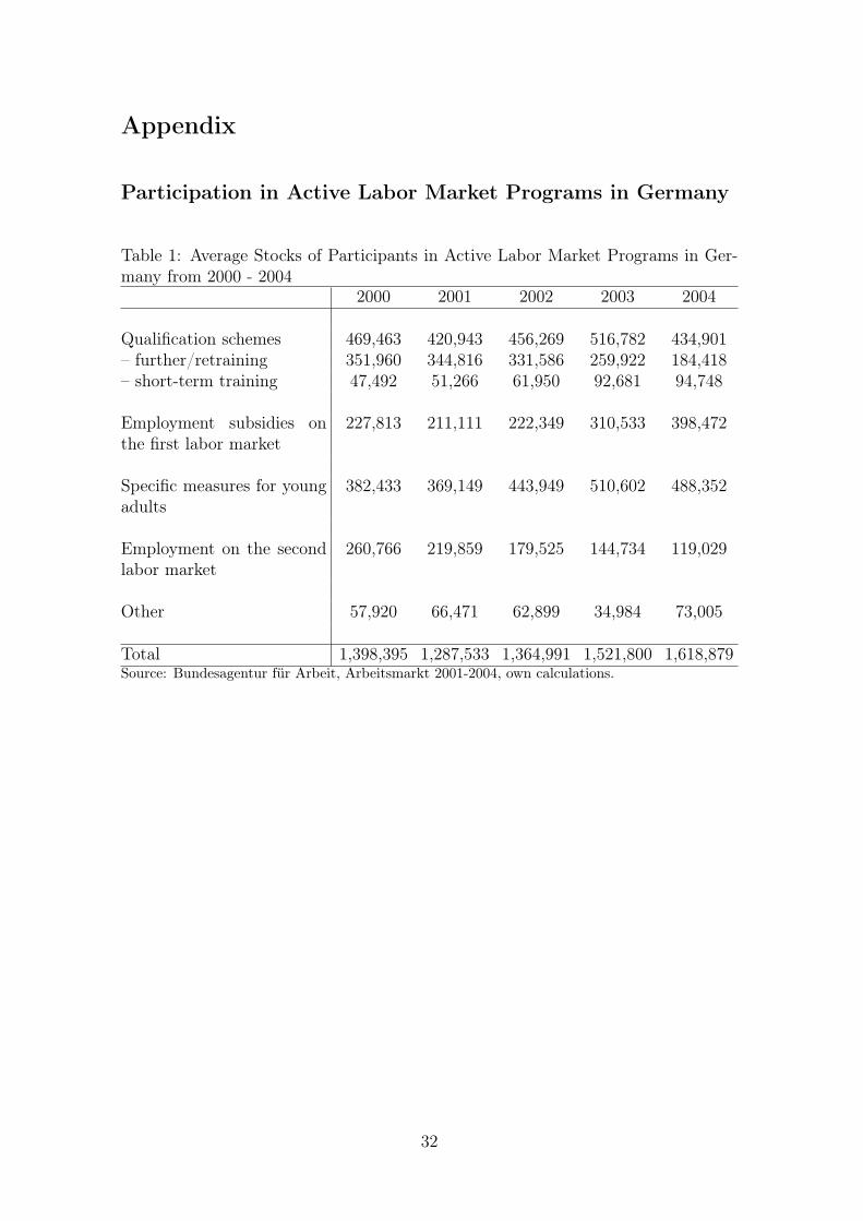
Appendix

Participation in Active Labor Market Programs in Germany

Table 1: Average Stocks of Participants in Active Labor Market Programs in Ger-many from 2000 - 2004

2000 2001 2002 2003 2004

Qualification schemes 469,463 420,943 456,269 516,782 434,901– further/retraining 351,960 344,816 331,586 259,922 184,418– short-term training 47,492 51,266 61,950 92,681 94,748

Employment subsidies onthe first labor market

227,813 211,111 222,349 310,533 398,472

Specific measures for youngadults

382,433 369,149 443,949 510,602 488,352

Employment on the secondlabor market

260,766 219,859 179,525 144,734 119,029

Other 57,920 66,471 62,899 34,984 73,005

Total 1,398,395 1,287,533 1,364,991 1,521,800 1,618,879Source: Bundesagentur für Arbeit, Arbeitsmarkt 2001-2004, own calculations.

32

Table 2: Entries into Active Labor Market Programs in Germany from 2000 - 20042000 2001 2002 2003 2004

Qualification schemes 1,153,720 1,069,409 1,457,047 1,502,166 1,548,439– further/retraining 551,534 449,622 456,301 254,718 185,041– short-term training 476,672 565,132 877,038 106,4293 1,188,369

Employment subsidies onthe first labor market

458,557 464,904 538,312 807,682 950,109

Placement and advisory ser-vices

601,281 742,065 947,098 1,460,170 2,566,780

Specific measures for youngadults

445,823 457,724 447,265 388,810 408,168

Employment on the secondlabor market

314,291 246,084 219,626 193,999 170,107

Other 391,122 515,670 453,224 21,283 309,446

Total 3,364,794 3,495,856 4,062,572 4,565,010 5,953,049Source: Bundesagentur für Arbeit, Arbeitsmarkt 2001-2004, own calculations.

Table 3: Average Expenditures per Participant in Short-term, Further and Retrain-ing in Germany from 2000-2003

2000 2001 2002 2003(1) (2) (1) (2) (1) (2) (1) (2)

Short-termtraining

580 1,2 570 1,1 658 0,9 538 1

Further/retrain-ing

1627 8,2 1668 9,3 1686 9,1 1555 10,5

– subsistence al-lowance

1152 1178 1188 1156

– training costs 640 664 681 631Note: Columns labeled with a (1) contain the average monthly expenditures (in Euro) per partic-ipant, columns labeled with a (2) display the average duration of the program in months. Source:Bundesagentur für Arbeit, Daten zu den Eingliederungsbilanzen 2000-2003.

33

Variable Definitions

Table 4: Variable Definitions

Name Definition

east 1 if place of residence is in East Germany (Berlin in-cluded), 0 otherwise

female 1 if female, 0 otherwiseagegroup age in 6 groupsforeigner 1 if citizenship is not German, 0 otherwiseethnicgerman 1 if ethnic German, i.e. returned settler from former

German settlements, 0 otherwisequalification 1 no degree, 2 vocational training degree, 3 university

or technical college degreeschooling 1 no schooling degree, 2 Hauptschulabschluss or Mit-

tlere Reife /Fachoberschule (degrees reached after com-pletion of the 9th or 10th grade), 3 Fachhochschulreifeor Abitur/Hochschulreife (degrees reached after comple-tion of the 12th or 13th grade)

health 1 no health problems mentioned, 2 health problems, butconsidered without impact on placement, 3 health prob-lems considered to have an impact on placement

pasthealth same categories as health, but referring to the past twoyears before the beginning of the unemployment spell

disabled 1 if disabled, 0 otherwiseland 16 categories for the German Bundesländerarea German Bundesländer aggregated into 6 categories. 1

SH, NI, HB, HH; 2 NW, 3 HE, RP, SL; 4 BY, BW; 5MV, BB, BE; 6 SN, ST, TH

region classification of the districts of residence according tolocal labor market conditions in 5 groups

family 1 missing, 2 living alone, 3 not married, but living to-gether with at least one person, 4 single parent, 5 mar-ried

married 1 missing, 2 married, 3 not marriedchild 1 if at least one child, 0 otherwise

<continued on next page>

34

Table 4: Variable Definitions <continued>

Name Definition

youngchild 1 if at least one child younger than 10 years, 0 otherwiseoccupation occupation of last employment in 7 categoriesindustry industry of last employment in 6 categoriesocchange 1 missing, 2 if the person wishes to work in the same

occupation as in the last employment, 3 otherwiseparttime 1 if the person worked less than full-time in the last

employment, 0 otherwisewhitecollar 2 if the previous employment was a white-collar job, 3

if it was a blue-collar job, 1 missingproblemgroup 1 if participation in a program with a social work com-

ponent within the last three years, 0 otherwiseonlyparttime 1 if information available that only part-time job is de-

sired, 0 otherwiseendlastjob 2 termination of last occupation by employer, 3 by em-

ployee, 4 limited in time, 5 other and missingquarter quarter of the end of the last employment (from 1 to 9)penalty 1 if the unemployed had a period of disqualification from

benefits within the last three years, 0 otherwisemotivationlack 1 if within the last three years there is information, that

the person did not appear regularly at the labor office,on lack of cooperation, availability or similar

pasttreatcancel 1 if abandonment of a program in the past according tothe benefit data, 0 otherwise

pastincapacity 1 if incapapacity of work due to illness, parental leave,cure or therapy within the last three years

proposals number of placement proposals divided by the days sincethe beginning of the unemployment spell and the startdate of the spell from which the information is taken

dapp 1 if employed as apprentice within the last three yearsbefore the beginning of the unemployment spell, 0 oth-erwise

<continued on next page>

35

Table 4: Variable Definitions <continued>

Name Definition

countemp, countub, counta,countsp, countoos, count-contact

number of days within the last three years before the be-ginning of unemployment spent in regular employment,receiving unemployment benefits, unemployment assis-tance, subsistance payment, out of sample, in contactwith the labor agency, respectively

demp6, demp12, demp24,demp6_12, demp12_24

1 if in regular employment 6, 12, 24, 6 and 12 and 12and 24 months, respectively, before the beginning of theunemployment spell

waged daily wage in the last job(s) before the beginning of theunemployment spell

ddssec, ddcens, ddmarg dummies if waged is censored: ddsec is 1 if earningsare within the social security thresholds, ddcens is 1 ifearnings are above the social security threshold, ddmargis 1 if earnings are below the social security threshold

lnwage, lnwagedsq log(waged) and log(waged) squared interacted withddssec

wage total wage in the last year before the beginning of theunemployment spell

dssec, dcens, dmarg censoring dummies referring to wage (see above)lnwage, lnwagesq log(wage) and log(wage) squared interacted with dssecur_yb, ur_qb, ur_qb3,ur_qb6, ur_qb12, ur_qb24

unemployment rate in the individual’s home district inthe calendar year before the beginning of unemploy-ment, in the last month of the quarter before the be-ginning of unemployment, and in the last month of thequarter before the beginning of the stratum, respectively

Note: If not mentioned otherwise, variables are defined relative to the beginning of the time window

of elapsed unemployment duration.

36

Sample Sizes and Descriptive Statistics for Selected Variables

Table 5: Sample SizesEast=0, Fem.=0 East=0, Fem.=1 East=1,Fem.=0 East=1, Fem.=1

Stratum 1 (0-3 Months)Waiting 29351 18409 15505 8538STT 912 693 621 368CFT 389 344 265 136



Aggregated Stratum 1 for PFT (0-12 Months)Waiting 25854 16060 12636 6614STT 2120 1593 1432 1013CFT 915 741 742 495PFT 263 234 145 98

37

Table 6: Descriptive Statistics for Selected VariablesVariable Mean SD Min Median Max

East=0, Female=0age 36.90053 7.718731 25 36 53foreigner .1736603 .378823 0 0 1schooling1 .1237411 .3292911 0 0 1schooling2 .7414522 .4378433 0 1 1schooling3 .1348067 .3415223 0 0 1qualification1 .3572672 .4792019 0 0 1qualification2 .5908243 .4916894 0 1 1qualification3 .0519085 .2218457 0 0 1countemp 801.0523 287.0826 86 873 1096




38

Figure 1: Density of Duration of Unemployment until Program Start0

.05

.1.1

5D

ensi

ty

0 5 10 15 20 25Months

East=0, Female=0

0.0

5.1

.15

.2D

ensi

ty

0 5 10 15 20 25Months

East=0, Female=1

0.0

5.1

.15

Den

sity

0 5 10 15 20 25Months

East=1, Female=0

0.0

5.1

Den

sity

0 5 10 15 20 25Months

East=1, Female=1Note: Calculations based on the sample of entrants into STT, CFT, and PFT.

39

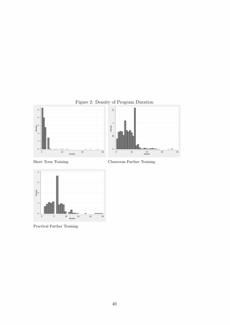
Figure 2: Density of Program Duration

0.1

.2.3

.4.5

Den

sity

0 10 20 30Months

Short Term Training

0.0

5.1

.15

Den

sity

0 10 20 30 40Months

Classroom Further Training

0.1

.2.3

.4D

ensi

ty

0 5 10 15 20 25Months

Practical Further Training

40

Estimated Employment Effects

Figure 3: Average Treatment Effect on the Treated (ATT) for STT, West Germany

−.0

50

.05

.1

−10 0 10 20Month

STT vs Waiting, East=0, Female=0, Stratum 1

−.1

−.0

50

.05

.1

−10 0 10 20Month


−.0

50

.05

.1.1

5

−10 0 10 20Month


−.0

50

.05

.1.1

5.2

−10 0 10 20Month


−.0

50

.05

.1

−10 0 10 20Month


−.0

50

.05

.1.1

5.2

−10 0 10 20Month


Difference in employment rates is measured on the ordinate, pre-unemployment (< 0) and post-treatment (≥ 0) months on the abscissa.

41

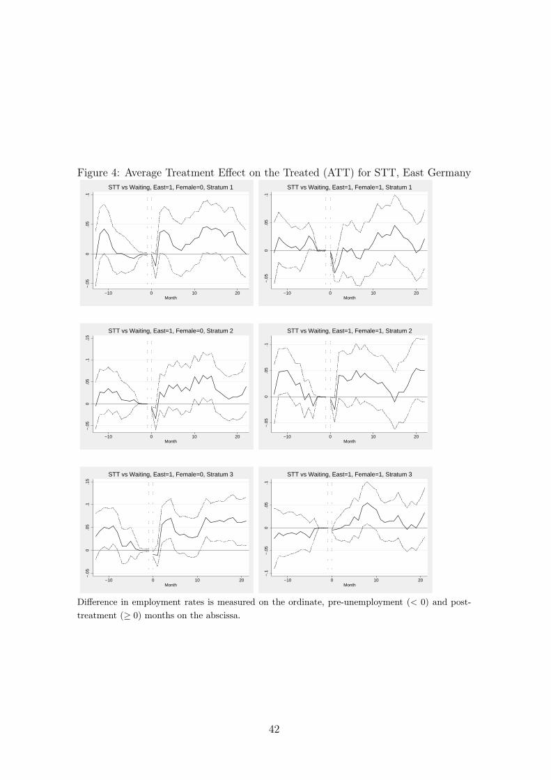
Figure 4: Average Treatment Effect on the Treated (ATT) for STT, East Germany

−.0

50

.05

.1

−10 0 10 20Month


−.0

50

.05

.1

−10 0 10 20Month


−.0

50

.05

.1.1

5

−10 0 10 20Month


−.0

50

.05

.1

−10 0 10 20Month


−.0

50

.05

.1.1

5

−10 0 10 20Month


−.1

−.0

50

.05

.1

−10 0 10 20Month



42

Figure 5: Average Treatment Effect on the Treated (ATT) for CFT, West Germany

−.3

−.2

−.1

0.1

−10 0 10 20Month

CFT vs Waiting, East=0, Female=0, Stratum 1

−.3

−.2

−.1

0.1

−10 0 10 20Month


−.2

−.1

0.1

−10 0 10 20Month


−.2

0.2

.4

−10 0 10 20Month


−.2

−.1

0.1

.2

−10 0 10 20Month


−.2

−.1

0.1

.2

−10 0 10 20Month



43

Figure 6: Average Treatment Effect on the Treated (ATT) for CFT, East Germany

−.3

−.2

−.1

0.1

.2

−10 0 10 20Month


−.2

−.1

0.1

−10 0 10 20Month


−.3

−.2

−.1

0.1

−10 0 10 20Month


−.2

−.1

0.1

.2

−10 0 10 20Month


−.2

−.1

0.1

.2

−10 0 10 20Month


−.2

−.1

0.1

−10 0 10 20Month



44

Figure 7: Average Treatment Effect on the Treated (ATT) for PFT, West and EastGermany

−.2

−.1

0.1

−10 0 10 20Month

PFT vs Waiting, East=0, Female=0, Stratum 1−

.2−

.10

.1.2

−10 0 10 20Month

PFT vs Waiting, East=0, Female=1, Stratum 1

−.3

−.2

−.1

0.1

.2

−10 0 10 20Month


−.2

−.1

0.1

.2

−10 0 10 20Month



45

Employment Eﬀects of Short and Medium Term Further ... · The IEBS collects information from four...

Documents

Transcript of Employment Eﬀects of Short and Medium Term Further ... · The IEBS collects information from four...