Empirical Return Periods of the Most Intense Vapor Transports during HistoricalAtmospheric River Landfalls on the U.S. West Coast

MICHAEL D. DETTINGERa

U.S. Geological Survey, Carson City, Nevada, and Center for Western Weather and Water Extremes, Scripps Institution of

Oceanography, La Jolla, California

F. MARTIN RALPHb

Center for Western Weather and Water Extremes, Scripps Institution of Oceanography, La Jolla, California

JONATHAN J. RUTZc

NOAA/NWS/Western Region Science and Technology Integration Division, Salt Lake City, Utah

(Manuscript received 2 January 2018, in final form 12 June 2018)

ABSTRACT

Atmospheric rivers (ARs) come in all intensities, and clear communication of risks posed by individual

storms in observations and forecasts can be a challenge. Modest ARs can be characterized by the percentile

rank of their integrated water vapor transport (IVT) rates compared to past ARs. Stronger ARs can be

categorized more clearly in terms of return periods or, equivalently, historical probabilities that at least one

ARwill exceed a given IVT threshold in any given year. Based on a 1980–2016 chronology of AR landfalls on

the U.S. West Coast from NASA’s Modern-Era Retrospective Analysis for Research and Applications,

version 2 (MERRA-2), datasets, the largest instantaneous IVTs—greater than 1700 kgm21 s21—have oc-

curred inARsmaking landfall between 418 and 468Nwith return periods longer than 20 years. IVT values with

similar return periods are smaller to the north and, especially, to the south (declining to ;750 kgm21 s21).

The largest storm-sequence IVT totals have been centered near 42.58N,with scatter among the top few events,

and these large storm-sequence totals dependmore on sequence duration than on the instantaneous IVT that

went into them. Maximum instantaneous IVTs are largest in the Pacific Northwest in autumn, with largest

IVT values arriving farther south as winter and spring unfold, until maximum IVTs reachNorthern California

in spring.

1. Introduction

Atmospheric rivers (ARs; Zhu and Newell 1998) are

naturally occurring, transitory, long (.2000km), narrow

(;850km) streams of intensewater vapor transport through

the lower atmosphere (,3km above sea level; Ralph et al.

2004;Guan andWaliser 2017). ARs over the northeast

Pacific conduct massive amounts of water vapor (anywhere

from 5 to 25 times the average flow of the Mississippi River

into theGulf ofMexico) through the atmospheric armof the

extratropical water cycle (Ralph and Dettinger 2011),

often connecting tropical and extratropical moisture

sources to the U.S. West Coast (Cordeira et al. 2013).

When theseARs encounterWestCoastmountain ranges,

they are uplifted and cooled, producing heavy rain and

snow (Neiman et al. 2002; Guan et al. 2010), providing

20%–50%of total precipitation in the Pacific Coast states

(Dettinger et al. 2011; Rutz et al. 2014).

The most intense ARs produce massive amounts of

precipitation on the West Coast states. Among the largest

storms in California’s history—storms that producedmore

than 400mm of precipitation within 3 days—92% have

been ARs (Ralph and Dettinger 2012). In large part be-

cause of these precipitation totals, ARs have been the

dominant cause of historical floods along rivers of the

Denotes content that is immediately available upon publica-

tion as open access.

a ORCID: 0000-0002-7509-7332.b ORCID: 0000-0002-0870-6396.c ORCID: 0000-0003-4337-0071.

Corresponding author: M. D. Dettinger, mddettin@usgs.gov

AUGUST 2018 DETT I NGER ET AL . 1363

DOI: 10.1175/JHM-D-17-0247.1

� 2018 American Meteorological Society. For information regarding reuse of this content and general copyright information, consult the AMS CopyrightPolicy (www.ametsoc.org/PUBSReuseLicenses).

Pacific Northwest (PNW) and central and northern

California (Ralph et al. 2006; Dettinger and Ingram

2013; Neiman et al. 2011; Barth et al. 2017; Konrad and

Dettinger 2017), where over 80% of floods since 1950

have been attributable to strong ARs. The most intense

ARs have historically caused landslides, debris flows,

levee failures, erosion, and consequent societal impacts

(Dettinger and Ingram 2013; Florsheim and Dettinger

2015; Oakley et al. 2017; Young et al. 2017; Oakley et al.

2018). At the same time, though, strong landfalling ARs

have also brought about the termination from more

than 70% of historical droughts in Washington, with

AR-induced drought terminations falling off to the

south, to about 35% of drought terminations in southern

California (Dettinger 2013).

However, not all ARs produce these extreme precipi-

tation and flood conditions. Rather, ARs range between

very modest intensities [as measured by the amount of

vertically integrated water vapor transport (IVT) that

they conduct per meter of cross-sectional distance, in

kgm21 s21] and very strong intensities. The more water

vapor that anAR transports, themore precipitation it can

yield (e.g., Neiman et al. 2002, 2009; Ralph et al. 2013;

Guan andWaliser 2015), depending also on several other

characteristics of the storm, including (but not limited to)

the orientation of the transports relative to the steepest

ascents of the mountain ranges they encounter, stability

of the atmosphere, and closeness of air within the AR to

saturation with respect to vapor upon landfall. The least

intense ARs are unlikely to yield extreme precipitation

and are most often beneficial sources of moderate rains,

snowfalls, andwater resources of Pacific-state landscapes.

Thus, ARs range between largely beneficial and largely

hazardous (Ralph et al. 2017a, 2018, manuscript sub-

mitted to Bull. Amer. Meteor. Soc.), and the intensity of

an AR storm—which plays a dominant role in de-

termining where in this range an AR storm will fall—is

one of the most important characteristics that must be

communicated for forecasts of an AR landfall (Cordeira

et al. 2017). A natural way to describe the largest ARs to

the public and professionals alike is by comparison to

other, historical large ARs and their consequences, much

as one often describes or analogizes a current riverine

flood and its impacts with some specific past flood.

However, many stakeholders do not accurately recall

specific historical storms or floods (e.g., ‘‘the great storm/

floods of New Years 1997’’), and so—with some techni-

cal misgivings (e.g., Shepard 2015)—riverine floods are

categorized in terms of their estimated return periods

(or annual probabilities of exceedence) at least as often as

by reference to specific historical events.

With this communications issue in mind, this paper an-

alyzes historical IVTs in ARs making landfall on the U.S.

West Coast from a global atmospheric reanalysis dataset in

terms of simple rank percentiles for small to moderate

ARs, and in terms of historical return periods of annual-

maximum IVT values. The analysis allows strong ARs, in

records and forecasts, to be categorized across the full range

of AR intensities in terms of how often ARs of similar in-

tensity have occurred historically, thus allowing a sense of

‘‘how intense is this storm compared to all the other ones?’’

to be communicated in simple, quantitative terms.

2. Data

This analysis proceeds from chronologies of ARs on the

U.S.West Coast and their IVTs at landfall, as identified by

the application of themethod ofRutz et al. (2014) to long-

term global atmospheric reanalysis products. These re-

analysis products are detailed representations of the state

of the global atmosphere based on assimilation of avail-

able historical observations into a numerical weather

(forecast) model, with the version of that model held

fixed throughout the period of the analysis (Ghil and

Malanotte-Rizzoli 1991; Kalnay et al. 1996). The re-

analysis calculations yield time series of all atmospheric

variables and conditions simulated at every grid cell and

vertical level in the model, variables, and conditions that

are internally and dynamically consistent with each other,

with historical observations, and with the model’s gov-

erning equations. The observations may include surface

observations on land and sea, weather balloon and aircraft

observations, and satellite imagery to the extent that each

source is available at each reanalysis time step.

The reanalysis product that will be the primary focus

here is NASA’s Modern-Era Retrospective Analysis for

Research and Applications, version 2 (MERRA-2), re-

analysis (Gelaro et al. 2017; GMAO 2015), using 3-hourly

data on its 0.58 latitude 3 0.6258 longitude grid spanning

37 historical years (or 36water years,October–September)

during the satellite era (1981–2016). Corresponding results

from selected segments from two other reanalysis products

will be considered in section 4:

d the National Centers for Environmental Prediction–

National Center for Atmospheric Research (NCEP–

NCAR) Reanalysis-1 (Kalnay et al. 1996, and updates

thereto), which spans .65 years (1948–2012 considered

here) of historical conditions at 6-hourly time steps on a

spatially coarse 2.58 latitude and longitude grid, andd the part of one of the European Center for Medium-

RangeWeather Forecasts (ECMWF) interim reanalysis

(ERA-Interim; Dee et al. 2011) products used in Rutz

et al. (2014), on a 1.58 latitude and longitude grid, on

6-hourly time steps, and spanning 22 years of historical

conditions (1989–2010).Notably, ERA-Interimdatasets

1364 JOURNAL OF HYDROMETEOROLOGY VOLUME 19

are available at a variety of different resolutions, in-

cluding finer than that used herein, and over longer time

periods.We use this particular segment of the reanalysis

not to suggest that ERA-Interim could not be used in

the analyses to follow, but rather to provide a perspec-

tive on how the choice of datasets—specifically, the

choice of resolutions—affects results of our analyses of

MERRA-2 ARs.

Rutz et al.’s (2014) approach to identifyingARs in such

datasets evaluates global IVT fields from these reanalysis

datasets, with IVT calculated according to the method-

ologies of Neiman et al. (2008) andMoore et al. (2012) as

IVT521

g

ðptpb

qVhdp , (1)

where q is specific humidity, Vh is the horizontal wind

vector, g is the acceleration due to gravity, pb is

1000 hPa, and pt is 200 hPa. In order for the following

comparisons of AR IVTs in the three reanalyses to be as

consistent as possible (not all of the reanalyses consid-

ered provide internally derived IVTs) and to maintain

consistency with previous applications of Rutz et al.’s

(2014) method, all IVTs used in this study were calcu-

lated from humidities and winds on standard model

pressure levels at the standard 3- or 6-h model-output

time steps. A useful alternative for future studies might

be IVT values that the MERRA-2 system provides di-

rectly, which have the advantage that these internally

generated IVTs are calculated at all (internal) model

times steps and on all model vertical coordinates and not

just the standard output pressure levels. In a comparison

of instantaneous IVTs from the MERRA-2 datasets by

Shields et al. (2018, their Fig. S1), internally derived

IVTs did not differ substantially (less than about

1 kgm21 s21) from the IVTs used herein. Nonetheless,

the internally derived IVTs may be preferable over

coasts and mountains in the long run.

At each time step, Rutz et al.’s (2014) method iden-

tifies ARs as features in the global IVT fields that

are .2000km in length with IVT . 250 kgm21 s21

throughout. In the present study, AR arrivals on the

U.S.West Coast identified by application of this algo-

rithm to each time step (separately) in each of the three

reanalysis datasets were analyzed, and the IVT values of

the ARs as they encounter the West Coast were tabu-

lated and used to characterize the intensity of landfalling

ARs. Examples of IVT time series that result from these

calculations, along with the water-year maximum IVT

values, are shown in Fig. 1, for theMERRRA-2 grid cell

at 37.58N, 123.58E (offshore from San Francisco Bay,

California) and 48.58N, 126.258W (offshore from the

northern tip of the Olympic Peninsula inWashington). In

both series, annual-maximum IVT values range from

about 750–800kgm21 s21 to about 1300–1400kgm21 s21,

with considerable year-to-year variation and modest, if

any, trends or steps. (Trend and changepoint analyses will

be described briefly in the next section.)

These AR chronologies are Eulerian in character in

that individual ARs are not followed, as moving fea-

tures, through space and time. Instead AR conditions

overhead are identified and tabulated for each of the

grid cells closest to the West Coast. In this sense, the

term ‘‘AR storm sequence’’ used in later sections of this

paper refers to periods when AR conditions are con-

tinuously present overhead of the grid cell in question,

and not the life cycle of an individual AR moving

through the atmosphere.

3. Analysis approach

An example analysis of IVTs in all ARs making

landfall at selected latitudes along the U.S. West Coast

from 1980 to 2016, as identified in the MERRA-2

dataset, is summarized in Table 1, which lists percent-

ages of time that anARwith intensity surpassing various

thresholds has made landfall at selected latitudes along

FIG. 1. Vertically integrated 3-hourly water vapor transports

during atmospheric river conditions (black bars) over theMERRA-2

grid cell at (a) 48.58N, 126.258Wand (b) 37.58N, 1258Wfor the period

from 1 Oct 1980 through 30 Sep 2016; the red curve is a 365-day

moving average of 3-hourly values, yellow and green lines are linear

regression fits to all-AR IVTs and water-year maximum AR IVTs,

and blue triangles are water-year maximum IVT values.

AUGUST 2018 DETT I NGER ET AL . 1365

the U.S. West Coast. Maximum IVTs during nonover-

lapping 3-day periods were evaluated here in order to

avoid double counting IVTs from the same ARs (based

on typical lengths of AR landfalls over sites along the

U.S. West Coast; Ralph et al. 2013). Among identified

ARs, maximum IVTs were between 250kgm21 s21

[the minimum IVT for inclusion as an AR in Rutz et al.’s

(2014) methodology] and 500kgm21 s21 from 50% to

70% of the time, depending on landfall latitude. Maxi-

mum IVTs are greater than 875kgm21 s21 between 2%

and 8% of the time, with most such exceedences occur-

ring along the Northern California and Oregon coasts.

This configuration of IVTs generally reflects the patterns

of long-term mean and 95th percentile IVT over the

northeast Pacific Ocean described by Lavers et al. (2015),

wherein maximum IVT values have historically been fo-

cused along a line connecting 308N just south of Japan

to somewhere near 458N on the West Coast, with IVTs

declining otherwise to the north and south.

Notably, for ARs with the strongest IVTs, the landfalls

reported in Table 1 are so infrequent that the communi-

cations value of comparingARs in terms of IVTpercentiles

is reduced (e.g., how does one convey the difference

between a 2%and 3% storm?). Consequently, for stronger

ARs, which are the focus of this study, we draw lessons

from the methods typically used to characterize the largest

riverine floods. We thus focus on return periods, which are

generallymore intuitive to a nonscientific audience. Return

periods account better for year-to-year variations in AR

frequencies than do period-of-record percentiles. Return

periods are also a common descriptor in engineering and

planning designs, for example, in the form of ‘‘100-yr

storms’’ and other categorizations of risk and intensity.

Thus, in the remainder of this study, empirical esti-

mates of the return periods of ARs exceeding various

strong-AR IVT thresholds are quantified as a means for

communicating the strength of the largest AR storms

that have made landfall on the U.S. West Coast in recent

decades. The return periods are estimated from the time

series of annual-peak IVTs during landfalling ARs at each

landfall latitude (e.g., as in Fig. 1). First, for each water year

in a reanalysis dataset, the maximum 3- or 6-hourly IVT

value associated with an AR making landfall at a given lat-

itude or latitude band is identified. Then these annual-peak

IVTs are ranked, with a standard ‘‘plotting position’’ (rank

divided by N 1 1, where N is the length of the time series;

Makkonen 2006), and herein each annual maximum is then

plotted with its plotting position located along a normal

distribution on the x axis and its IVT value generally

plotted along a logarithmic scale on the y axis. Other

plotting/estimation approaches could have been used, so

that the lognormal plotting of the IVT maxima here is

somewhat arbitrary. However, Table 2 compares re-

gression fits when simple or logarithmic plotting-position

probabilities, normal or lognormal probabilities, and

Pearson type III or log-Pearson type III probabilities are

used. The table shows that all of the distributions provide

reasonable fits across the historical ranges of annual-

maximum IVT values. Our purpose here is not to provide

parametric estimates of return periods for extrapolations

beyond the historically observed range of values (to, e.g.,

100-yr storms well beyond our 22–65-yr-long records),

but rather to provide broad empirical estimates of return

periods for everyday communication purposes. The

identification of the most appropriate parametric distri-

butions (Carpenter and Bithell 2000) for extreme events

analysis of IVTs (as opposed to floods in surface rivers) is a

project for the future, and thus even the confidence limits

that are presented later are based on nonparametric boot-

strap resamplings of the observed IVT values. For engi-

neering and extrapolation purposes, much more intensive,

precise, and application-specific choices and fits of extreme-

value distributions (Interagency Advisory Committee on

Water Data 1982) will presumably be needed.

Calculated this way, the resulting return periods (or

recurrence intervals) are estimates of the inverse of the

TABLE 1. Percentages of historical nonoverlapping 3-day periods with at least oneAR landfall with 3-hourly IVTmaxima greater than the

indicated thresholds, in MERRA-2 fields, calendar years 1980–2016.

IVT thresholds

Landfall latitude 325 kgm21 s21 500 kgm21 s21 625 kgm21 s21 750 kgm21 s21 875 kgm21 s21 Maximum reported

498N 80% 38% 19% 9% 4% 1333 kgm21 s21

478N 79% 41% 23% 12% 5% 1552 kgm21 s21

458N 81% 45% 27% 15% 8% 1730 kgm21 s21

438N 80% 45% 27% 16% 8% 1619 kgm21 s21

418N 78% 38% 20% 10% 2% 1483 kgm21 s21

398N 74% 32% 17% 8% 4% 1299 kgm21 s21

378N 71% 30% 14% 6% 3% 1400 kgm21 s21

358N 67% 25% 11% 5% 2% 1244 kgm21 s21

338N 62% 21% 7% 2% 0.4% 879 kgm21 s21

1366 JOURNAL OF HYDROMETEOROLOGY VOLUME 19

probability that a given IVT intensity will be equaled or

exceeded in any given year. This attention to the largest

IVT values each year allows us to focus on characteriz-

ing just the largest and most hazardous ARs, without

‘‘dilution’’ by the differing numbers of modest ARs at

the various latitudes or by occasions when multiple

strong ARs arrive in some years.

4. Choice of reanalysis dataset

As noted previously, reanalysis datasets available to

identify and characterize AR landfalls differ in their

spatial resolutions and in their periods of record. To

estimate long-term frequencies, or probabilities, of the

strongest historical ARs, a longer record (larger sample

size) is generally much preferred. But how does the

spatial resolution of a given reanalysis dataset impact

the maximum IVTs reported? That is, are maximum

IVTs blurred and muted in a lower-resolution product

compared to those in a higher resolution dataset? If so,

then the higher-resolution dataset might be needed even

if its period of record is smaller than a coarse resolution

but longer alternative.

Before reporting and discussing return periods of AR

intensities in the MERRA-2 chronology (which became

the focus of this study), AR IVTs and annual-maximum

AR IVTs in theMERRA-2were compared to those in the

longer but coarser Reanalysis-1 AR chronology. These

comparisons weremade to provide a sense of the effects of

coarsening spatial resolutions on reported IVT values and

on estimated AR-IVT return periods. To improve further

our sense of the effect of grid scale on reanalysis IVT

values, a short but intermediate-resolutionAR chronology

used by Rutz et al. (2014) and based on a part of ERA-

Interim is also included in this comparison.

First, IVT values for every 6-hourly time step during a

22-yr period (1989–2010) that was available in all three

of the AR chronologies were compared at three grid

cells near the U.S. West Coast. Six-hourly values were

used because this was the finest temporal resolution

common to all three reanalysis chronologies. Grid cells

were chosen to be as close to each other as possible (near or

at 358, 408, and 458N), which meant choosing grid cells

closest to the 2.58 Reanalysis-1 grid cells just offshore at

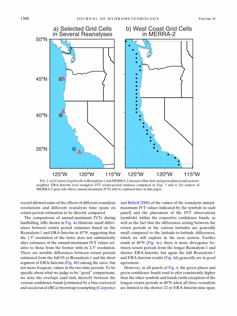
those latitudes (Fig. 2a). Figure 3 compares IVT values

from the three reanalyses during every 6-hourly time step in

the 22-yr period that coincided with AR conditions in the

MERRA-2AR chronology.At each latitude,AR IVTs for

the three chronologies tend to be very similar to each other

for the AR time steps with weak to modest IVT intensity

(as indicated by comparisons of the dashedone-to-one lines

to the regression lines in each panel of Fig. 3). For time

steps with more intense (.500kgm21 s21) AR conditions,

the coarser reanalyses yield lower IVTvalues. The slopes of

each of the regression lines in Fig. 3 are significantly less

than a one-to-one relation with theMERRA-2 IVT values,

suggesting that, when addressing strong IVTs, the spatial

resolution of the reanalysis used to characterize ARs mat-

ters. The finerMERRA-2 resolution yields IVT values that

are roughly about 25% higher than the coarser reanalyses.

Five subsets from the three reanalysis chronologies

were also analyzed to compare estimates of return

periods at the grid cells nearest those just offshore in

Reanalysis-1:

1) Return periods were estimated from the full 65-yr

Reanalysis-1 AR chronology spanning the 1948–

2012 period.

2) Then return periods were re-estimated from the same

chronology but using only values from the 22-yr 1989–

2010 period spanned by the shorter ERA-Interim

chronology.

3) Return periods were estimated from those 22 years

of ERA-Interim AR chronology.

4) Return periods were estimated using a 6-hourly

resampling of the 3-hourly MERRA-2 AR chronol-

ogy during its full 37-yr period of record.

5) Finally, MERRA-2 return periods are estimated

based on only ARs during the shorter 22-yr ERA-

Interim period.

This comparison of return-period estimates using the

various reanalysis chronologies and various periods of

TABLE 2. Coefficients of determination (regression r2) of annual-maximum 3-hourly IVT values during ARs, water years 1981–2016, in

MERRA-2AR chronology at selectedWest Coast landfall latitudes, for return-period fits vs simple plotting-position odds [rank/(361 1)],

normal probabilities, and Pearson type III probabilities, and logarithms of the IVTs vs the same three sets of probabilities. All fits are

statistically strong (p� 0.0001) and all yield similar return-period estimates within the historical range of IVT maxima.

Landfall latitude Odds vs IVT Odds vs log(IVT)

Normal probs

vs IVT

Normals

vs log(IVT)

Pearson probabilities

vs IVT

Pearson probabilities

vs log(IVT)

358N 96% 97% 97% 98% 97% 99%

408N 95% 97% 97% 99% 98% 99%

458N 78% 84% 86% 86% 91% 93%

AUGUST 2018 DETT I NGER ET AL . 1367

record allowed some of the effects of different reanalysis

resolutions and different reanalysis time spans on

return-period estimation to be directly compared.

The comparisons of annual-maximum IVTs during

landfalling ARs shown in Fig. 4a illustrate small differ-

ences between return period estimates based on the

Reanalysis-1 and ERA-Interim at 458N, suggesting that

the 1.58 resolution of the latter does not substantially

alter estimates of the annual-maximum IVT values rel-

ative to those from the former with its 2.58 resolution.There are notable differences between return periods

estimated from the full 65-yr Reanalysis-1 and the short

segment of ERA-Interim (Fig. 4b) among the rarer, but

not more frequent, values in the two time periods. To be

specific about what we judge to be ‘‘good’’ comparisons,

we note the overlaps (and lack thereof) between the

various confidence bands [estimated by a bias-corrected

and accelerated (BCa) bootstrap resampling (Carpenter

and Bithell 2000) of the values of the reanalysis annual-

maximum IVT values indicated by the symbols in each

panel] and the placement of the IVT observations

(symbols) within the respective confidence bands, as

well as the fact that the differences arising between the

return periods at the various latitudes are generally

small compared to the latitude-to-latitude differences,

which we will explore in the next section. Farther

south at 408N (Fig. 4c), there is more divergence be-

tween return periods from the longer Reanalysis-1 and

shorter ERA-Interim, but again the full Reanalysis-1

and ERA-Interim results (Fig. 4d) generally are in good

agreement.

However, in all panels of Fig. 4, the green pluses and

green confidence bands tend to plot consistently higher

than the other symbols and bands (with exception of the

longest return periods at 408N when all three reanalysis

are limited to the shorter 22-yr ERA-Interim time span;

FIG. 2. (a) Centers of grid cells in Reanalysis-1 andMERRA-2 datasets (blue dots and green pluses) and nearest-

neighbor ERA-Interim (red triangles) IVT return-period analyses compared in Figs. 3 and 4; (b) centers of

MERRA-2 grid cells where annual-maximum IVTs will be explored later in this paper.

1368 JOURNAL OF HYDROMETEOROLOGY VOLUME 19

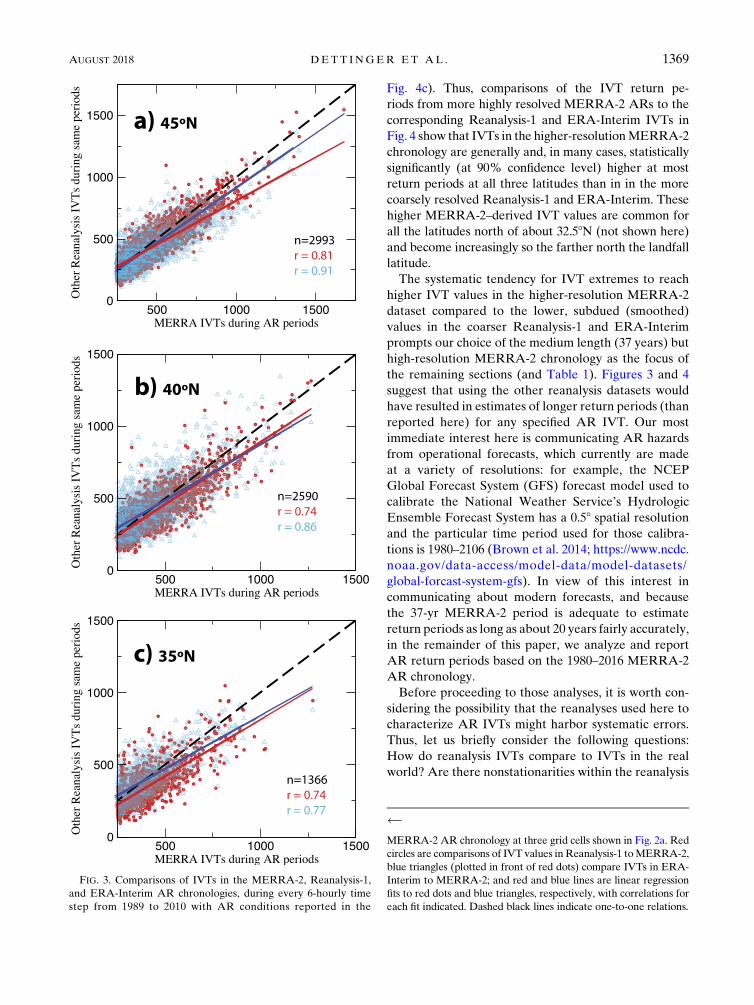
Fig. 4c). Thus, comparisons of the IVT return pe-

riods from more highly resolved MERRA-2 ARs to the

corresponding Reanalysis-1 and ERA-Interim IVTs in

Fig. 4 show that IVTs in the higher-resolutionMERRA-2

chronology are generally and, in many cases, statistically

significantly (at 90% confidence level) higher at most

return periods at all three latitudes than in in the more

coarsely resolved Reanalysis-1 and ERA-Interim. These

higher MERRA-2–derived IVT values are common for

all the latitudes north of about 32.58N (not shown here)

and become increasingly so the farther north the landfall

latitude.

The systematic tendency for IVT extremes to reach

higher IVT values in the higher-resolution MERRA-2

dataset compared to the lower, subdued (smoothed)

values in the coarser Reanalysis-1 and ERA-Interim

prompts our choice of the medium length (37 years) but

high-resolution MERRA-2 chronology as the focus of

the remaining sections (and Table 1). Figures 3 and 4

suggest that using the other reanalysis datasets would

have resulted in estimates of longer return periods (than

reported here) for any specified AR IVT. Our most

immediate interest here is communicating AR hazards

from operational forecasts, which currently are made

at a variety of resolutions: for example, the NCEP

Global Forecast System (GFS) forecast model used to

calibrate the National Weather Service’s Hydrologic

Ensemble Forecast System has a 0.58 spatial resolutionand the particular time period used for those calibra-

tions is 1980–2106 (Brown et al. 2014; https://www.ncdc.

noaa.gov/data-access/model-data/model-datasets/

global-forcast-system-gfs). In view of this interest in

communicating about modern forecasts, and because

the 37-yr MERRA-2 period is adequate to estimate

return periods as long as about 20 years fairly accurately,

in the remainder of this paper, we analyze and report

AR return periods based on the 1980–2016 MERRA-2

AR chronology.

Before proceeding to those analyses, it is worth con-

sidering the possibility that the reanalyses used here to

characterize AR IVTs might harbor systematic errors.

Thus, let us briefly consider the following questions:

How do reanalysis IVTs compare to IVTs in the real

world? Are there nonstationarities within the reanalysis

FIG. 3. Comparisons of IVTs in the MERRA-2, Reanalysis-1,

and ERA-Interim AR chronologies, during every 6-hourly time

step from 1989 to 2010 with AR conditions reported in the

MERRA-2 AR chronology at three grid cells shown in Fig. 2a. Red

circles are comparisons of IVT values inReanalysis-1 toMERRA-2,

blue triangles (plotted in front of red dots) compare IVTs in ERA-

Interim to MERRA-2; and red and blue lines are linear regression

fits to red dots and blue triangles, respectively, with correlations for

each fit indicated. Dashed black lines indicate one-to-one relations.

AUGUST 2018 DETT I NGER ET AL . 1369

datasets that would invalidate temporal analyses? First,

several recent studies have made comparisons of ARs

depicted in reanalysis datasets with direct airborne mea-

surements of these storms in order to document the

validity of reanalysis AR properties (Guan and Waliser

2017; Ralph et al. 2017b; Guan et al. 2018). Taken

together, based on the 21 dropsonde-observed ARs

between 1998 and 2016, these studies conclude that

reanalysis IVTs are generally accurate with mean errors

less of21% inMERRA-2 (13% in ERA-Interim). This

result validates the use of ARs detected in reanalysis

datasets and the IVT values in those reanalyses.

Despite these encouraging checks on reanalysis IVTs,

reanalyses are known to harbor discontinuities associ-

ated with changes in the sources (types, provenances,

spatial densities, and temporal frequencies) of data input

to the reanalysis procedures [e.g., as reported in Gelaro

et al. (2017) for MERRA-2, in Dee et al. (2011) for

ERA-Interim, and as implied by the major input

changes between the presatellite era and satellite era in

FIG. 4. Comparisons of return-period estimates of annual-maximum 6-hourly IVTs in landfalling ARs, based on

(a),(c),(e) the 22-yr period from 1989 to 2010 and (b),(d),(f) full-chronology periods [indicated in (b)], from AR

chronologies for three reanalyses, at three grid cells along the U.S.West Coast (Fig. 2a). Symbols are the reanalysis

IVT estimates at each return period; color bands are the 90%confidence limits for each based onBCa resampling of

the return periods. In order to accommodate overlapping confidence bands, the outer edges of each color band are

presented as thin curves in a slightly darker hue.

1370 JOURNAL OF HYDROMETEOROLOGY VOLUME 19

Reanalysis-1 of Kalnay et al. (1996)]. Such discontinuities

could violate one of the assumptions underlying quanti-

tative estimates of return periods, that is, that the series

analyzed are statistically stationary (e.g., Interagency

Advisory Committee on Water Data 1982). To evaluate

the range of discontinuities present in the datasets used

here, tests were performed to detect possible change-

points in 5-yr mean IVTs during all AR landfalls in the

MERRA-2 AR chronology. These series are erratic

enough, and interannually variable enough (Fig. 1), so

that many possible changepoints were detected at 95%

confidence level. However, the scales of these potential

discontinuities were uniformly small in the study domain,

from32.58 to 49.58N,with 5-yrmean changes large enough to

be possible changepoints, averaged at each latitude, ranging

between 26 and 14kgm21 s21 (from 21.4% to 10.9%

change) depending on latitude, and themaximum5-yrmean

changes at the various latitudes falling between 240

and 140kgm21 s21 (610%). Similar tests for change-

points in 5-yr variances (Levene 1960) of AR IVTs were

also performed; the largest potential changepoints

among5-yr standarddeviations ranged from645kgm21 s21

at any latitude in the present study domain. Thus, al-

though subtle discontinuities are likely present in re-

analysis IVTs, they appear to be small (in MERRA-2)

compared to the range of annual-maximum IVTs that

will be analyzed here.

However, another kind of nonstationarity—a long-

term trend—is now known to be present in historical AR

IVTs on the West Coast. Gershunov et al. (2017)

describe a long-term trend inWest Coast IVTs identified

in the NOAA Twentieth Century Reanalysis (Compo

et al. 2011), with increasing IVT and precipitation to the

north along the West Coast and declines to the south,

apparently tied to long-term warming of the tropical

Western Pacific and a poleward migration of storm

tracks. Figure 5 illustrates trends in the MERRA-2

3-hourly and annual-maximum IVT values series at all

of theWest Coast grid cells (locations in Fig. 2b) that are

the primary focus of this paper. When all AR landfalls

are analyzed, overall trends are extremely small in

magnitude, but in the annual-maximum IVT series, the

overall trends range from 2120 to 1150 kgm21 s21

along the West Coast. Only at 48.58N does this change

rise to a level that would pass a two-sided 95% signifi-

cance test amidst the large year-to-year variability in

these maximum IVTs (e.g., see Fig. 1a). Nonetheless,

the fitted trends in Fig. 5 are quite coherent with latitude

and are large enough in magnitude to suggest that they

are present. The estimated magnitude of the trend rec-

ommends that return periods for annual-maximum

IVT estimated here may err by 6100–150kgm21 s21,

or roughly 10%.

5. Geography of AR return periods

Focusing then on the full 3-hourly, 0.58 latitude 30.6258 longitude, MERRA-2 dataset and AR chronol-

ogy for water years 1981–2016, Fig. 6 shows empirical

estimates of return periods of annual-maximum AR

IVT values at six locations (from among the grid cells in

Fig. 2b) and in four latitude bands along the U.S. West

Coast. On a latitude-by-latitude basis (Figs. 6a,b), north

of about 37.58N, landfall IVTs associated with the range

of return periods shown fall within a relatively narrow

range of values, although within that band IVTs at 458Nare consistently the largest shown. Generally though,

north of about 37.58N, an annual-maximum IVT value

of about 1000kgm21 s21 is exceeded every 1.5–2 years,

and annual-maximum values greater than about

1250kgm21 s21 occur about every 7 years. From 37.58Nsouthward to 32.58N, annual-maximum IVT values fall

off quickly, so that at 32.58N, a maximum-annual IVT

value with 1.5-yr return period is only 600 kgm21 s21

and a 20-yr annual-maximum IVT is still less than

1000kgm21 s21.

The solid curves in Fig. 6c show return periods for

annual-maximum IVTs during AR landfalls anywhere

within four latitude bands along the West Coast. The

solid black curve shows return periods for AR landfalls

occurring anywhere along the West Coast in any given

year, whereas the solid blue curve shows return periods

for AR landfalls anywhere between 428 and 508N(roughly anywhere along the Oregon or Washington

coast lines). Because, as noted previously, the largest

IVT maxima have occurred at and around 458N, these

two curves (blue and black) are very similar. Annual-

maximum IVTs along the Northern California coast

(green curve) are generally about 10% lower than those

FIG. 5. Overall linear trends in annual-maximum IVTs during

AR landfalls (bars), at any time (black curve), and during any AR

landfalls (dashed red curve), as a function of West Coast latitude

(locations shown in Fig. 2b), in MERRA-2 AR chronology, 1980–

2016. Overall trends are differences in linearly regressed IVTs at

the beginning of 1980 and at the end of 2016. A null hypothesis that

the maximum-annual IVT trends falling within the cyan and gray

bands are different from zero cannot be rejected at 95% and 99%

levels, respectively.

AUGUST 2018 DETT I NGER ET AL . 1371

(at the same return periods) along the Oregon–Washington

coast.Annual-maximumIVTsalong theSouthernCalifornia

coast (red curve) range from 30% to 40% less than the other

bands and echo the values at the northern limits of this band,

for example, at 358N.A more complete representation of the geographic

distribution of annual-maximum IVT return periods is

shown in Fig. 7a. As in Fig. 6 and in general accordance

with the historical patterns of IVT over the northeast

Pacific shown by Lavers et al. (2015), the largest annual-

maximum West Coast IVT values encountered have

occurred near 458N (palest pink area in Fig. 7a) with

values greater than 1700kgm21 s21. Annual-maximum

IVT values with largest return periods (;20 years) de-

cline to the north and south. IVT values with much

shorter return periods (e.g., ;1.5 years) are, of course,

much smaller (,1000kgm21 s21) everywhere but also

obtain the largest values near (just south of) 458N.At the

southernmost latitudes shown in Fig. 7a, IVT values with

roughly 1-yr return periods are less than 500kgm21 s21.

6. Storm-sequence vapor-transport total returnperiods

The maximum instantaneous (3-hourly) IVT values

discussed thus far can give indications of resulting

maximum precipitation intensities (Neiman et al. 2002,

2009; Ralph et al. 2013; Guan and Waliser 2015), which

are relevant to predictions of flood or inundation peaks

in some small catchments and to some erosion and

Earth-movement processes and risks. For flood predic-

tion in even moderately large catchments and other

hazards, though, duration of an AR landfall and pre-

cipitation over a given location can be at least as im-

portant (Ralph et al. 2013; Lamjiri et al. 2017). Thus,

another metric that is now used to characterize ARs is

the time-integrated storm-sequence total-IVT amount

[measured in kgm21; paralleling storm-total strategies

used by Ralph et al. (2013) and Lamjiri et al. (2017)] at a

given location. In this analysis, these storm totals are

computed, in an Eulerian sense, as the time-integrated

IVT total that passes overhead of the location during

each time period (storm) when AR conditions contin-

uously are present above that location. For the very

large AR ‘‘storm’’ totals considered here, which include

durations as long as 6 days, these uninterrupted AR

FIG. 6. Historical return periods (and probabilities of exceedence)

and confidence bands of water-year annual-maximum AR rates of

IVT in 3-hourly periods at selected (a),(b) latitudes and (c) latitude

bands along the U.S. West Coast (from among the black dots on

maps in Fig. 2b), based on MERRA-2, water years 1981–2016.

Symbols are MERRA-2 annual-maximum IVT values; color bands

represent the 90% confidence limits fromBCa bootstrap resampling

(as in Fig. 4), with upper and lower limits indicated by thin curves

along with bootstrapped estimates of median return periods in-

dicated by a third (central) curve. In (c), West Coast band spans

32.58–508N; Oregon–Washington, 42.58–508N; Northern California,

368–428N; and Southern California, 32.58–35.58N.

1372 JOURNAL OF HYDROMETEOROLOGY VOLUME 19

conditions almost certainly do not represent a single AR

arrival but rather are likely to consist of storm sequences

of multiple ARs.

Figure 7b shows the geographic distribution along the

U.S. West Coast of return periods of annual-maximum

storm-sequence total-IVT amounts. Unlike instantaneous

IVT (with its observed maximum near 458N), the largest

West Coast annual-maximum AR storm-total IVT

values in the MERRA-2 chronology (.303 107 kgm21

with return period. 20 years) have historically occurred

near 37.58 and 47.58N. Notably, this double-peaked

distribution of 20-yr storm-total IVTs is restricted

to the large, rarest storm sequences, and so may reflect

scatter associated with the limitations of estimating

20-yr return periods using time series only 37 years long.

To test this interpretation, a similar analysis (not shown)

wasmade of the 65-yr-longReanalysis-1 AR chronology

discussed in section 4. With that longer time series,

storm sequences with return periods of 10–30 years are

better sampled, and the double-peaked distribution for

these larger, rarer storm sequences does not emerge.

Instead, the peak near 37.58N remains but the apparent

peak at 47.58N disappears when 28 more years are

included in the analysis.

For storm totals with return periods less than about

5 years, the storm-total maxima are largest near 428–458N(Oregon coast), with 1.25-yr storm totals rising to about

12 3 107 kgm21 there and with the smallest 1.25-yr

values occurring at the southern limit of this analysis

where 1.25-yr IVT values decline to ,2 3 107 kgm21.

FIG. 7. Historical return periods (and exceedence probabilities) of (a) annual-maximum IVT transport rates and

(b) annual-maximum storm totals in landfallingARs, water years 1981–2016, along theU.S.West Coast at grid cells

indicated by black dots in maps along right-hand side of the panels, based on MERRA-2.

AUGUST 2018 DETT I NGER ET AL . 1373

The durations and IVT rates that combine to yield

these large return-period storm sequences are illustrated

in Fig. 8. Figure 8a shows IVT totals mapped in Fig. 7b, as

averaged over return-period bands from 2 to 3 years and

from 10 to 30 years. The double peak noted earlier in

Fig. 7b for the longest return-period storm sequences is

evident in Fig. 8a, as is the simpler geographic distribution

for shorter return periods. For each annual-maximum

storm sequence that contributed to Figs. 7b and 8a, du-

rations, storm-maximum IVT rates, and IVT averaged

over the entire storm sequence are shown in Figs. 8b and

8c, respectively. Storm-average IVT rates aremore or less

the same (with 610% scatter) between sequences with

10–30-yr and 2–3-yr return periods from 32.58 to 428N,

with large storm sequences north of 428N exhibiting

10%–20% larger average intensities (Fig. 8c). At most

latitudes, the maximum instantaneous-IVT rates during

the storm sequences with .10-yr return periods are

mostly modestly (10%–30%) stronger than those in se-

quences with 2–3-yr return periods (Fig. 8d).Durations of

the .10-yr return-period sequences range from 25% (at

42.58N) to 140% (338N) longer than durations of the

storm sequences with 2–3-yr return periods (Fig. 7b). The

peak in 10–30-yr IVT totals near 37.58N results from

several very long-duration storm sequences (also found in

theReanalysis-1), whereas the apparent peak near 47.58N(not substantiated by analysis of the Reanalysis-1) arose

from a combination of larger storm-average IVT and

perhaps some longer-duration sequences there. Overall,

though, almost all of the increase in storm-sequence IVT

totals with long return periods, which range from 40% to

150% larger, over the storm sequences with shorter

return periods arise from differences in their respective

durations (see also Lamjiri et al. 2017).

7. Seasonality of AR return periods

The ARs associated with these annual-maximum

IVTs make their landfalls at different times of year.

To illustrate the seasonality of the AR IVT maxima,

Fig. 9 shows return periods of IVT maxima as a function

of month and latitude. Thus, the first column in Fig. 9a

shows the instantaneous IVT values that would be

exceeded, on average, once in every 20 Septembers at

each latitude along the U.S. West Coast, the second

column for once in every 20 Octobers, and so on.

Figure 9b highlights similar results, but for IVTs with

5 September return periods, 5 October returns, and so

on. Summer AR IVTs are not shown here because, as

documented by Neiman et al. (2008) and acknowledged

by many subsequent studies (e.g., Rutz et al. 2014),

summer IVT features that are AR-like do not generally

produce significant rainfall in the western United States.

The geographic patterns of IVT seasonality are broadly

similar for the two panels in Fig. 9, with—for a given

return period—largest annual-maximum IVT values ar-

riving in early autumn in the PNW (north of about 438N,

north of California). The maximum IVT values then

occur farther south as winter approaches and arrives. By

midwinter (December–January), the 20-yr IVT maxima

(Fig. 9a) are largest between about 408 and 438N, and then

the locations of themaximum IVT values drift southward

FIG. 8. Latitudinal distribution of (a) the annual-maximum storm-sequence total vapor transport with return

periods from 2 to 3 years and from 10 to 30 years, (b) the duration of these same storm sequences, (c) the average

IVT over the entire storm sequence, and (d) the maximum instantaneous IVT during the storm sequence, for ARs

or uninterrupted sequences of ARs making landfall along the U.S. West Coast, water years 1981–2016.

1374 JOURNAL OF HYDROMETEOROLOGY VOLUME 19

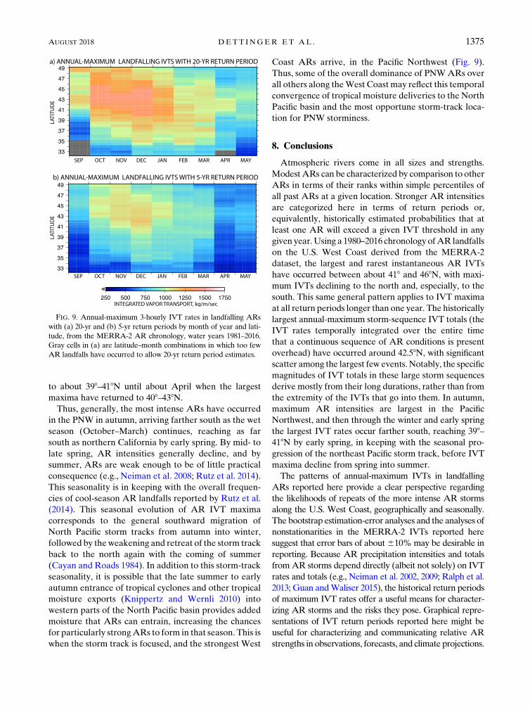
to about 398–418N until about April when the largest

maxima have returned to 408–438N.

Thus, generally, the most intense ARs have occurred

in the PNW in autumn, arriving farther south as the wet

season (October–March) continues, reaching as far

south as northern California by early spring. By mid- to

late spring, AR intensities generally decline, and by

summer, ARs are weak enough to be of little practical

consequence (e.g., Neiman et al. 2008; Rutz et al. 2014).

This seasonality is in keeping with the overall frequen-

cies of cool-season AR landfalls reported by Rutz et al.

(2014). This seasonal evolution of AR IVT maxima

corresponds to the general southward migration of

North Pacific storm tracks from autumn into winter,

followed by theweakening and retreat of the storm track

back to the north again with the coming of summer

(Cayan and Roads 1984). In addition to this storm-track

seasonality, it is possible that the late summer to early

autumn entrance of tropical cyclones and other tropical

moisture exports (Knippertz and Wernli 2010) into

western parts of the North Pacific basin provides added

moisture that ARs can entrain, increasing the chances

for particularly strongARs to form in that season. This is

when the storm track is focused, and the strongest West

Coast ARs arrive, in the Pacific Northwest (Fig. 9).

Thus, some of the overall dominance of PNWARs over

all others along theWest Coast may reflect this temporal

convergence of tropical moisture deliveries to the North

Pacific basin and the most opportune storm-track loca-

tion for PNW storminess.

8. Conclusions

Atmospheric rivers come in all sizes and strengths.

ModestARs can be characterized by comparison to other

ARs in terms of their ranks within simple percentiles of

all past ARs at a given location. Stronger AR intensities

are categorized here in terms of return periods or,

equivalently, historically estimated probabilities that at

least one AR will exceed a given IVT threshold in any

given year.Using a 1980–2016 chronology ofAR landfalls

on the U.S. West Coast derived from the MERRA-2

dataset, the largest and rarest instantaneous AR IVTs

have occurred between about 418 and 468N, with maxi-

mum IVTs declining to the north and, especially, to the

south. This same general pattern applies to IVT maxima

at all return periods longer than one year. The historically

largest annual-maximum storm-sequence IVT totals (the

IVT rates temporally integrated over the entire time

that a continuous sequence of AR conditions is present

overhead) have occurred around 42.58N, with significant

scatter among the largest few events. Notably, the specific

magnitudes of IVT totals in these large storm sequences

derive mostly from their long durations, rather than from

the extremity of the IVTs that go into them. In autumn,

maximum AR intensities are largest in the Pacific

Northwest, and then through the winter and early spring

the largest IVT rates occur farther south, reaching 398–418N by early spring, in keeping with the seasonal pro-

gression of the northeast Pacific storm track, before IVT

maxima decline from spring into summer.

The patterns of annual-maximum IVTs in landfalling

ARs reported here provide a clear perspective regarding

the likelihoods of repeats of the more intense AR storms

along the U.S. West Coast, geographically and seasonally.

The bootstrap estimation-error analyses and the analyses of

nonstationarities in the MERRA-2 IVTs reported here

suggest that error bars of about610%may be desirable in

reporting. Because AR precipitation intensities and totals

fromAR storms depend directly (albeit not solely) on IVT

rates and totals (e.g., Neiman et al. 2002, 2009; Ralph et al.

2013; Guan andWaliser 2015), the historical return periods

of maximum IVT rates offer a useful means for character-

izing AR storms and the risks they pose. Graphical repre-

sentations of IVT return periods reported here might be

useful for characterizing and communicating relative AR

strengths in observations, forecasts, and climate projections.

FIG. 9. Annual-maximum 3-hourly IVT rates in landfalling ARs

with (a) 20-yr and (b) 5-yr return periods by month of year and lati-

tude, from the MERRA-2 AR chronology, water years 1981–2016.

Gray cells in (a) are latitude–month combinations in which too few

AR landfalls have occurred to allow 20-yr return period estimates.

AUGUST 2018 DETT I NGER ET AL . 1375

Acknowledgments. We are grateful for helpful com-

ments from Chris Konrad (USGS) and three anonymous

reviewers that improved this paper markedly. M.D.’s re-

search was supported by theU.S. Geological Survey’s Earth

System Processes Division, Water Cycle Branch, and a co-

operative arrangementwith SonomaCountyWaterAgency.

F.M.R.’s contributions at the Center for Western Weather

and Water Extremes (CW3E) were supported by the

California Department of Water Resources and by the U.S.

Army Corps of Engineers (USACE) Engineer Research

and Development Center–Cooperative Ecosystem Studies

Unit (CESU) as part of Forecast Informed Reservoir Op-

erations (FIRO) under Grant W912HZ-15-2-0019. The AR

and IVT chronologies used in this study can be obtained

from http://www.inscc.utah.edu/;rutz/ar_catalogs/.

REFERENCES

Barth, N. A., G. Villarini, M. A. Nayak, and K.White, 2017: Mixed

populations and annual flood frequency estimates in the

western United States. Water Resour. Res., 53, 257–269,

https://doi.org/10.1002/2016WR019064.

Brown, J. D., L. Wu, M. He, S. Regonda, H. Lee, and D.-J. Seo, 2014:

Verificationof temperature, precipitation, and streamflow forecasts

from the NOAA/NWS Hydrologic Ensemble Forecast Service

(HEFS): 1.Experimental designand forcingverification. J.Hydrol.,

519, 2869–2889, https://doi.org/10.1016/j.jhydrol.2014.05.028.

Carpenter, J., and J. Bithell, 2000: Bootstrap confidence intervals:

When, which, what? A practical guide for medical statisti-

cians. Stat. Med., 19, 1141–1164, https://doi.org/10.1002/(SICI)

1097-0258(20000515)19:9,1141::AID-SIM479.3.0.CO;2-F.

Cayan, D. R., and J. O. Roads, 1984: Local relationships between

United States West Coast precipitation and monthly mean circu-

lation parameters.Mon.Wea.Rev., 112, 1276–1282, https://doi.org/

10.1175/1520-0493(1984)112,1276:LRBUSW.2.0.CO;2.

Compo, G. P., and Coauthors, 2011: The Twentieth Century Re-

analysis Project.Quart. J. Roy. Meteor. Soc., 137, 1–28, https://

doi.org/10.1002/qj.776.

Cordeira, J. M., F.M. Ralph, and B. J.Moore, 2013: The development

and evolution of two atmospheric rivers in proximity to western

North Pacific tropical cyclones in October 2010.Mon. Wea. Rev.,

141, 4234–4255, https://doi.org/10.1175/MWR-D-13-00019.1.

——,——,A.Martin, N. Gaggini, R. Spackman, P. Neiman, J. Rutz,

and R. Pierce, 2017: Forecasting atmospheric rivers during

CalWater 2015. Bull. Amer. Meteor. Soc., 98, 449–459, https://

doi.org/10.1175/BAMS-D-15-00245.1.

Dee, D. P., and Coauthors, 2011: The ERA-Interim reanalysis: Con-

figuration and performance of the data assimilation system.Quart.

J. Roy. Meteor. Soc., 137, 553–597, https://doi.org/10.1002/qj.828.

Dettinger, M. D., 2013: Atmospheric rivers as drought busters on

the U.S. West Coast. J. Hydrometeor., 14, 1721–1732, https://

doi.org/10.1175/JHM-D-13-02.1.

——, and B. L. Ingram, 2013: The coming megafloods. Sci. Amer.,

308, 64–71, https://doi.org/10.1038/scientificamerican0113-64.

——, F. M. Ralph, T. Das, P. J. Neiman, and D. Cayan, 2011: At-

mospheric rivers, floods, and the water resources of California.

Water, 3, 445–478, https://doi.org/10.3390/w3020445.Florsheim, J., and M. Dettinger, 2015: Promoting atmospheric-

river and snowmelt fueled biogeomorphic processes by re-

storing river-floodplain connectivity in California’s Central

Valley. Geomorphic Approaches to Integrated Floodplain

Management of Lowland Fluvial Systems in North America

and Europe, P. Hudson and H. Middelkoop, Eds., Springer,

119–141, https://doi.org/10.1007/978-1-4939-2380-9_6.

Gelaro, R., and Coauthors, 2017: The Modern-Era Retrospective

Analysis for Research and Applications, version 2 (MERRA-2).

J.Climate,30, 5419–5454, https://doi.org/10.1175/JCLI-D-16-0758.1.

Gershunov, A., T. Shulgina, F. M. Ralph, D. A. Lavers, and J. J. Rutz,

2017: Assessing the climate-scale variability of atmospheric rivers

affecting western North America. Geophys. Res. Lett., 44, 7900–

7908, https://doi.org/10.1002/2017GL074175.

Ghil, M., and P. Malanotte-Rizzoli, 1991: Data assimilation in

meteorology and oceanography.Advances inGeophysics, Vol.

33, Academic Press, 141–266, https://doi.org/10.1016/S0065-

2687(08)60442-2.

GMAO, 2015: MERRA-2 inst3_3d_asm_Np: 3d, 3-hourly, in-

stantaneous, pressure-level, assimilation, assimilated meteo-

rological fields V5.12.4. GES DISC, accessed 30 July 2018,

https://doi.org/10.5067/QBZ6MG944HW0.

Guan, B., andD. E.Waliser, 2015: Detection of atmospheric rivers:

Evaluation and application of an algorithm for global studies.

J. Geophys. Res. Atmos., 120, 12 514–12 535, https://doi.org/

10.1002/2015JD024257.

——, and ——, 2017: Atmospheric rivers in 20 year weather

and climate simulations: A multimodel, global evaluation.

J. Geophys. Res. Atmos., 122, 5556–5581, https://doi.org/

10.1002/2016JD026174.

——, N. P. Molotch, D. E. Waliser, E. J. Fetzer, and P. J.

Neiman, 2010: Extreme snowfall events linked to atmo-

spheric rivers and surface air temperature via satellite

measurements. Geophys. Res. Lett., 37, L20401, https://doi.

org/10.1029/2010GL044696.

——, D. E. Waliser, and F. M. Ralph, 2018: An intercomparison be-

tween reanalysis and dropsonde observations of the total water

vapor transport in individual atmospheric rivers. J.Hydrometeor.,

19, 321–337, https://doi.org/10.1175/JHM-D-17-0114.1.

InteragencyAdvisory Committee onWaterData, 1982: Guidelines

for determining flood flow frequency. Bulletin 17B of the

Hydrology Subcommittee, 183 pp., https://www.fema.gov/

media-library/assets/documents/8403.

Kalnay, E., and Coauthors, 1996: The NCEP/NCAR 40-Year Re-

analysis Project. Bull. Amer. Meteor. Soc., 77, 437–471, https://

doi.org/10.1175/1520-0477(1996)077,0437:TNYRP.2.0.CO;2.

Knippertz, P., and H. Wernli, 2010: A Lagrangian climatol-

ogy of tropical moisture exports to the Northern Hemi-

sphere extratropics. J. Climate, 23, 987–1003, https://doi.

org/10.1175/2009JCLI3333.1.

Konrad, C. P., and M. D. Dettinger, 2017: Flood runoff in relation

to water vapor transport by atmospheric rivers over the

western United States, 1949–2015. Geophys. Res. Lett., 44,

11 456–11 462, https://doi.org/10.1002/2017GL075399.

Lamjiri, M. A., M. D. Dettinger, F. M. Ralph, and B. Guan, 2017:

Hourly storm characteristics along the U.S. West Coast: Role

of atmospheric rivers in extreme precipitation. Geophys. Res.

Lett., 44, 7020–7028, https://doi.org/10.1002/2017GL074193.

Lavers, D. A., F. M. Ralph, D. E. Waliser, A. Gershunov, and

M. D. Dettinger, 2015: Climate change intensification of hor-

izontal vapor transport in CMIP5. Geophys. Res. Lett., 42,

5617–5625, https://doi.org/10.1002/2015GL064672.

Levene, H., 1960: Robust tests for equality of variances. Contri-

butions to Probability and Statistics: Essays in Honor of

Harold Hotelling, I. Olkin et al., Eds., Stanford University

Press, 278–292.

1376 JOURNAL OF HYDROMETEOROLOGY VOLUME 19

Makkonen, L., 2006: Plotting positions in extreme value anal-

ysis. J. Appl. Meteor. Climatol., 45, 334–340, https://doi.

org/10.1175/JAM2349.1.

Moore, B. J., P. J. Neiman, F. M. Ralph, and F. E. Barthold, 2012:

Physical processes associated with heavy flooding rainfall in

Nashville,Tennessee, andvicinity during1–2May2010:The roleof

anatmospheric river andmesoscale convective systems.Mon.Wea.

Rev., 140, 358–378, https://doi.org/10.1175/MWR-D-11-00126.1.

Neiman, P. J., F. M. Ralph, A. B. White, D. E. Kingsmill, and P. O.

Persson, 2002: The statistical relationship between upslope flow

and rainfall in California’s coastal mountains: Observations dur-

ing CALJET. Mon. Wea. Rev., 130, 1468–1492, https://doi.org/10.1175/1520-0493(2002)130,1468:TSRBUF.2.0.CO;2.

——,——,G.A.Wick, J. D. Lundquist, andM.D.Dettinger, 2008:

Meteorological characteristics and overland precipitation

impacts of atmospheric rivers affecting the West Coast of

North America based on eight years of SSM/I satellite ob-

servations. J. Hydrometeor., 9, 22–47, https://doi.org/10.1175/

2007JHM855.1.

——, A. B. White, F. M. Ralph, D. J. Gottas, and S. I. Gutman,

2009: A water vapour flux tool for precipitation forecasting.

Proc. Inst. Civ. Eng.: Water Manage., 162, 83–94, https://doi.

org/10.1680/wama.2009.162.2.83.

——, L. J. Schick, F. M. Ralph, M. Hughes, and G. A. Wick, 2011:

Flooding in western Washington: The connection to atmo-

spheric rivers. J. Hydrometeor., 12, 1337–1358, https://doi.org/10.1175/2011JHM1358.1.

Oakley, N. S., J. T. Lancaster, M. L. Kaplan, and F. M. Ralph, 2017:

Synoptic conditions associated with cool-season post-fire debris

flows in the Transverse Ranges of southern California. Nat.

Hazards, 88, 327–354, https://doi.org/10.1007/s11069-017-2867-6.

——, ——, B. J. Hatchett, J. Stock, F. M. Ralph, S. C. Roj, and

S. Lukashov, 2018: A 22-yr climatology of cool season hourly

precipitation conducive to shallow landslides in California.

Earth Interact., 22, https://doi.org/10.1175/EI-D-17-0029.1.

Ralph, F. M., and M. D. Dettinger, 2011: Storms, floods and the

science of atmospheric rivers. Eos, Trans. Amer. Geophys.

Union, 92, 265–266, https://doi.org/10.1029/2011EO320001.

——, and ——, 2012: Historical and national perspectives on ex-

treme West Coast precipitation associated with atmospheric

rivers during December 2010. Bull. Amer. Meteor. Soc., 93,783–790, https://doi.org/10.1175/BAMS-D-11-00188.1.

——, P. J. Neiman, and G. A. Wick, 2004: Satellite and CALJET

aircraft observations of atmospheric rivers over the eastern

North Pacific Ocean during the El Niño winter of 1997/98.

Mon. Wea. Rev., 132, 1721–1745, https://doi.org/10.1175/

1520-0493(2004)132,1721:SACAOO.2.0.CO;2.

——, ——, ——, S. Gutman, M. Dettinger, D. Cayan, and A. B.

White, 2006: Flooding on California’s Russian River: Role of

atmospheric rivers. Geophys. Res. Lett., 33, L13801, https://doi.org/10.1029/2006GL026689.

——,T. Coleman, P. J. Neiman, R. J. Zamora, andM.D.Dettinger,

2013: Observed impacts of duration and seasonality of

atmospheric-river landfalls on soil moisture and runoff in

coastal northern California. J. Hydrometeor., 14, 443–459,

https://doi.org/10.1175/JHM-D-12-076.1.

——, and Coauthors, 2017a: Atmospheric rivers emerge as a global

science and applications focus. Bull. Amer. Meteor. Soc., 98,

1969–1973, https://doi.org/10.1175/BAMS-D-16-0262.1.

——, and Coauthors, 2017b: Dropsonde observations of total in-

tegrated water vapor transport within North Pacific atmo-

spheric rivers. J. Hydrometeor., 18, 2577–2596, https://doi.org/

10.1175/JHM-D-17-0036.1.

Rutz, J. J., W. J. Steenburgh, and F.M. Ralph, 2014: Climatological

characteristics of atmospheric rivers and their inland pene-

tration over the western United States. Mon. Wea. Rev., 142,

905–921, https://doi.org/10.1175/MWR-D-13-00168.1.

Shepard, M., 2015: What does a ‘100 or 1000-year’ rain event ac-

tually mean? Forbes, 5 October, https://www.forbes.com/sites/

marshallshepherd/2015/10/05/what-does-a-100-or-1000-year-

flood-actually-mean/#6c6ce5601fb4.

Shields C. A., and Coauthors, 2018: Atmospheric River Tracking

Method Intercomparison Project (ARTMIP): Project goals

and experimental design. Geosci. Model Dev., 11, 2455–2474,

https://doi.org/10.5194/gmd-11-2455-2018.

Young, A.M., K. T. Skelly, and J.M. Cordeira, 2017: High-impact

hydrologic events and atmospheric rivers in California: An

investigation using the NCEI Storm Events Database. Geo-

phys. Res. Lett., 44, 3393–3401, https://doi.org/10.1002/

2017GL073077.

Zhu, Y., and R. E. Newell, 1998: A proposed algorithm for mois-

ture fluxes from atmospheric rivers. Mon. Wea. Rev., 126,

725–735, https://doi.org/10.1175/1520-0493(1998)126,0725:

APAFMF.2.0.CO;2.

AUGUST 2018 DETT I NGER ET AL . 1377