Eos, Vol. 76, No. 2, January 10, 1995

GPS stations within the stippled area in Fig­ure 1 (that is, SLR velocities are not included in the pole determination). This rotation re­sults in velocities at the NAF of about 25 mm/yr.

As indicated by the residual velocities in Figure 3, deviations from uniform plate mo­tion appear to increase toward the Hellenic arc. The overall pattern suggests crustal ex­tension in the southern Aegean Sea and western Turkey. Crustal extension in this re­gion is generally consistent with independent GPS results from the southern Aegean [KastensetaL, 1993] as well as with earthquake focal mechanisms and geologic structure [McKenzie, 1970; Sengor et at., 1985]. However, the observed stretching rate (10 mm/yr) is considerably less than the over­all Anatolian plate motion rate and less than one third of the rates derived from analysis of earthquake data [McKenzie, 1970]. The small magnitude of the residual velocities in­dicates that this region behaves approximately as a coherent plate (Ana­tolian plate). The fit between the small circle about this GPS pole and the NAF (Figure 3) provides independent support for this pole lo­cation and indicates that the NAF represents the principal boundary between the Ana­tolian and Eurasian plates. Additional GPS measurements are planned over the next few years, and the much improved space and ground components of the GPS promise to

A Singular-Spectrum Analysis (SSA) Toolkit is now available for use on comput­ers with X-windows capabilities. The Toolkit provides free, compact, and easy access to SSA and several powerful spectral analysis techniques not readily available in common statistical packages. The current Toolkit, Ver­sion 1.1, provides tools for

Michael D. Dettinger, U.S. Geological Survey, Water Resources Division, 5735 Kearney Villa Rd., San Diego, CA 92123; Michael Ghil and Christopher M. Strong, Institute of Geophysics and Planetary Physics, University of Califor­nia, Los Angeles, CA 90024; William Weibel, Department of Atmospheric Sciences, Univer­sity of California, Los Angeles; CA 90024; Pascal Yiou, Laboratiore de Moderation du Climat et de 1'Environment, Commissariat a l'£nergie Atomique, Gif-sur-Yvette, France

substantially improve our understanding of kinematic and dynamic processes affecting this area of active continental deformation.

Acknowledgments

The GPS measurements reported in this study were supported by UNAVCO and ac­complished in coordination with independent surveys by the Institute fur Ange-wandte Geodasie, Frankfurt, Germany, Eidgenossiche Technische Hochschule-Zu-rich, Switzerland, and Durham University, Durham, England, under the direction of the General Command of Mapping, Ankara, Tur­key. We are grateful to each of these organizations for cooperation in data acquisi­tion and analysis. Many individuals participated in the field observations, and we acknowledge their important contribution to this project. This research was supported in part by NSF grant EAR-8709461, NASA grant NAGW-1961, and the Turkish Ministry of Na­tional Defense, General Command of Mapping. Partial support for M. B. Oral came through a fellowship from the Ministry of Edu­cation, Turkey.

References

DeMets, C , R.G. Gordon., D. F. Argus, and S. Stein, Current plate motions, Geophys. J. Int., 101, 425, 1990.

• breaking down univariate, possibly nonstationary time series into trends, peri­odic oscillations, other statistically significant components, and noise;

• reconstructing the contributions of se­lected components to the time series; and

• estimating power spectra of the time series or any of its components by modern spectral methods. These results are achieved through the SSA, complemented by other spectral estimation tools that include correlograms, the Multi-Ta­per Method (MTM), and the Maximum En­tropy Method (MEM). The philosophy of the Toolkit is that only simultaneous application of several spectral methods provides reliable information on a given time series. The Toolkit is readily extended to new methods but is not expected to become an all-purpose

Isacks, B., J. Oliver, and L.R. Sykes, Seismol­ogy and the new global tectonics, J. Geo­phys. Res., 73, 5855, 1968.

Jackson, J., and D. McKenzie, The relation­ship between plate motions and seismic mo­ment tensors, and the rates of active deformation in the Mediterranean and Mid­dle East, Geophys. J. R. Astron. Soc, 93, 45, 1988.

Kastens, K. A., L. E. Gilbert, K. J. Hurst, H. Billiris, D. Paradissis, G. Veis, W. Hoppe, and W. Schluter, GPS evidence for arc-paral­lel extension along the Hellenic arc, south­ern Aegean sea, Greece, Geol. Soc. Am. Abstracts with Program, A242, 1993.

McKenzie, D. P., Plate tectonics of the Medi­terranean region, Nature, 226, 239, 1970.

Molnar, P., and P. Tapponnier, Cenozoic tec­tonics of Asia: effects of a continental colli­sion, Science, 189, 419, 1975.

Oral, B., Global Positioning System (GPS) Measurements in Turkey (1988-1992): Kinematics of the Africa-Arabia-Eurasia Plate Collision Zone, Ph.D. thesis, Mass. Inst, of Technol., Cambridge, 344 pp., 1994.

Sengor, A. M. C , N. Goriir, and F. Saroglu, Strike-slip faulting and related basin forma­tion in zones of tectonic escape: Turkey as a case study, in Strike-slip Faulting and Basin Formation, edited by K.T. Biddle and N. Christie-Blick, Soc. of Econ. Paleon-tol. Min. Sec. Publ., p. 37, 1985.

Smith, D. E., R. Kolenkiewicz, J. W. Robbins, P. J. Dunn, and M. H. Torrence, Horizontal crustal motion in the central and eastern Mediterranean inferred from Satellite Laser Ranging measurements, Geophys. Res. Lett., 21, 1979, 1994.

package. General statistical packages, such as SAS or Matlab, are not as easy to use or ex­pand and do not contain the particularly powerful combination of time series analysis tools found in the SSA Toolkit. The Toolkit is being distributed by the Department of At­mospheric Sciences at the University of Cali-

fnput Signal

H

0.0

-2.0

3 - Kll'.;̂ 1900

****

*^L}«r>>.

Fig. 1. Toolkit menu and SOI time-series plot, with months from January 1933 on the ab­scissa and dimensionless SOI values on the or­dinate. Original color image appears at back of this volume.

Software Expedites Singular-Spectrum Analysis of Noisy Time Series PAGE 12,14,21

Michael D. Dettinger, Michael Ghil, Christopher M. Strong, William Weibel, and Pascal Yiou

This page may be freely copied.

Eos, Vol. 76, No. 2, January 10, 1995

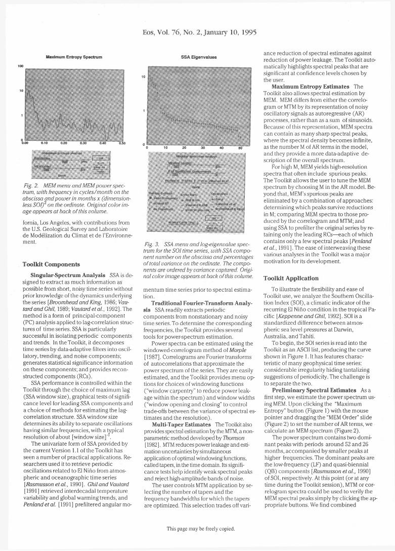
Fig. 2. MEM menu and MEM power spec­trum, with frequency in cycles/month on the abscissa and power in months x (dimension-less SOI)2 on the ordinate. Original color im­age appears at back of this volume.

fornia, Los Angeles, with contributions from the U.S. Geological Survey and Laboratoire de Modelization du Climat et de l'Environne-ment.

Toolkit Components

Singular-Spectrum Analysis SSA is de­signed to extract as much information as possible from short, noisy time series without prior knowledge of the dynamics underlying the series [Broomhead and King, 1986; Vau-tardandGhil, 1989; Vautardetai, 1992].The method is a form of principal-component (PC) analysis applied to lag-correlation struc­tures of time series. SSA is particularly successful in isolating periodic components and trends. In the Toolkit, it decomposes time series by data-adaptive filters into oscil­latory, trending, and noise components; generates statistical significance information on these components; and provides recon­structed components (RCs).

SSA performance is controlled within the Toolkit through the choice of maximum lag (SSA window size), graphical tests of signifi­cance level for leading SSA components and a choice of methods for estimating the lag-correlation structure. SSA window size determines its ability to separate oscillations having similar frequencies, with a typical resolution of about [window size] .

The univariate form of SSA provided by the current Version 1.1 of the Toolkit has seen a number of practical applications. Re­searchers used it to retrieve periodic oscillations related to El Nino from atmos­pheric and oceanographic time series [RasmussonetaL, 1990]. Ghil and Vautard [1991] retrieved interdecadal temperature variability and global warming trends, and Penlandetal. [1991] prefiltered angular mo-

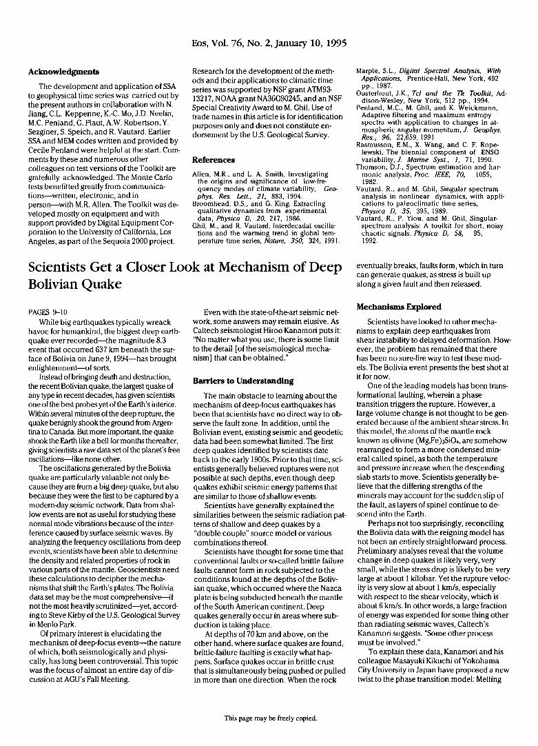
Fig. 3. SSA menu and log-eigenvalue spec­trum for the SOI time series, with SSA compo­nent number on the abscissa and percentages of total variance on the ordinate. The compo­nents are ordered by variance captured. Origi­nal color image appears at back of this volume.

mentum time series prior to spectral estima­tion.

Traditional Fourier-Transform Analy­sis SSA readily extracts periodic components from nonstationary and noisy time series. To determine the corresponding frequencies, the Toolkit provides several tools for power-spectrum estimation.

Power spectra can be estimated using the windowed-correlogram method of Marple [1987]. Correlograms are Fourier transforms of autocorrelations that approximate the power spectrum of the series. They are easily estimated, and the Toolkit provides menu op­tions for choices of windowing functions ("window carpentry" to reduce power leak­age within the spectrum) and window widths ("window opening and closing" to control trade-offs between the variance of spectral es­timates and the resolution).

Multi-Taper Estimates The Toolkit also provides spectral estimation by the MTM, a non-parametric method developed by Thomson [1982]. MTM reduces power leakage and esti­mation uncertainties by simultaneous application of optimal windowing functions, called tapers, in the time domain. Its signifi­cance tests help identify weak spectral peaks and reject high-amplitude bands of noise.

The user controls MTM application by se­lecting the number of tapers and the frequency bandwidths for which the tapers are optimized. This selection trades off vari­

ance reduction of spectral estimates against reduction of power leakage. The Toolkit auto­matically highlights spectral peaks that are significant at confidence levels chosen by the user.

Maximum Entropy Estimates The Toolkit also allows spectral estimation by MEM. MEM differs from either the correlo-gram or MTM by its representation of noisy oscillatory signals as autoregressive ( A R ) processes, rather than as a sum of sinusoids. Because of this representation, MEM spectra can contain as many sharp spectral peaks, where the spectral density becomes infinite, as the number M of AR terms in the model, and they provide a more data-adaptive de­scription of the overall spectrum.

For high M, MEM yields high-resolution spectra that often include spurious peaks. The Toolkit allows the user to tune the MEM spectrum by choosing M in the AR model. Be­yond that, MEM's spurious peaks are eliminated by a combination of approaches: determining which peaks survive reductions in M; comparing MEM spectra to those pro­duced by the correlogram and MTM; and using SSA to prefilter the original series by re­taining only the leading RCs—each of which contains only a few spectral peaks [Penland et al., 1991 ] . The ease of interweaving these various analyses in the Toolkit was a major motivation for its development.

Toolkit Application

To illustrate the flexibility and ease of Toolkit use, we analyze the Southern Oscilla­tion Index (SOI), a climatic indicator of the recurring El Nino condition in the tropical Pa­cific [Keppenne and Ghil, 1992]. SOI is a standardized difference between atmos­pheric sea level pressures at Darwin, Australia, and Tahiti.

To begin, the SOI series is read into the Toolkit as an ASCII list, producing the curve shown in Figure 1. It has features charac­teristic of many geophysical time series: considerable irregularity hiding tantalizing suggestions of periodicity. The challenge is to separate the two.

Preliminary Spectral Estimates As a first step, we estimate the power spectrum us­ing MEM. Upon clicking the "Maximum Entropy" button (Figure 1) with the mouse pointer and dragging the "MEM Order" slide (Figure 2) to set the number of AR terms, we calculate an MEM spectrum (Figure 2) .

The power spectrum contains two domi­nant peaks with periods around 52 and 26 months, accompanied by smaller peaks at higher frequencies. The dominant peaks are the low-frequency (LF) and quasi-biennial (QB) components [Rasmusson etai, 1990] of SOI, respectively. At this point (or at any time during the Toolkit session), MTM or cor­relogram spectra could be used to verify the MEM spectral peaks simply by clicking the ap­propriate buttons. We find combined

This page may be freely copied.

*os, Vol. 76, No. 2, January 10, 1995

nents 1-4; same units as in Figure lb. (b) MEM power spectrum of the SSA-filtered time series shown in (a); same units as in Figure 2. Original color image appears at back of this volume.

application of different spectral methods more enlightening than relying on variance estimates from a single one.

SSA Decomposition SSA can be ap­plied to the data to extract the oscillatory components, to display the variability they represent, or to remove noise prior to re­newed spectral estimation. The resulting Toolkit menu and SSA eigenvalue spectrum appear in Figure 3. As in other PC analyses, each SSA eigenvalue is equal to the variance captured by the corresponding component, and structured signals typically rise above the flat tail of the eigenvalue spectrum that represents noise. Vautard and Ghil [ 1989] showed that oscillatory parts of a time series are isolated by pairs of SSA components with nearly equal eigenvalues. The eigenvalue spectrum (Figure 3) shows two leading pairs of nearly equal eigenvalues: 1-2 and 3-4; they are found to correspond, indeed, to oscilla­tions. The Toolkit display includes ad hoc error bars to account for sampling effects on eigenvalue estimation; these bars help the user evaluate breaks in spectral slope be­tween signal and noise and potential pairing of eigenvalues. The Toolkit also offers op­tions for estimating eigenvalue sampling errors by Monte Carlo simulations of either white [Ghil and Vautard, 1991; Vautard etai, 1992] orAR [Allen and Smith, 1994] noise.

SSA decomposition into oscillations, trends, and noise is achieved in terms of tem­poral empirical-orthogonal functions (T-EOFs) and temporal PCs (T-PCs), that are recurring temporal patterns and their time-varying amplitudes, respectively. These representations can be examined by clicking the T-EOFs" or MT-PCs" buttons (Figure 3) . In this brief illustration, we jump ahead to re­construct the leading oscillations by clicking on the "Filtered RCs" button and selecting for reconstruction the first four SSA compo­nents. The result is the filtered time series shown in Figure 4a; it captures the main fea­tures of the original one in Figure 1, while effectively removing the noisy part. Notice, in Figure 4a, the marked increase in amplitude of the filtered SOI series after 1970, following a lull in the mid-century. Information about the amplitude variations of oscillatory sig­nals, usually lost in standard spectral analyses, is an immediate output from SSA.

Finally, the RC series can be analyzed by any of the spectral estimators provided. The power spectrum of each RC is much simpler than that of the complete time series [Pen-land etai, 1991; Vautard etai, 1992].The MEM spectrum for the SSA-filtered series shown in Figure 4b displays an increase in the signal-to-noise ratio from 10 for the unfil-tered data (Figure 2) to 108 for the filtered data (Figure 4b). In this example, an initial MEM spectrum (Figure 2) showed peak power at 26 and 52 months. The use of SSA provided data-adaptive filters for the oscilla­tions (Figure 3) without having to search for some nominally optimal band pass filter. The leading oscillatory components were re­constructed (Figure 4a) and passed again through the maximum entropy analysis (Fig­ure 4b). The next step in such an analysis (not shown) is using the Toolkit to quickly explore the sensitivity of results to various MEM orders and SSA window lengths, to con­firm the MEM spectrum by application of other spectral estimators [Vautard etai, 1992] or to investigate other SSA components above the noise level in Figure 3.

Toolkit Availability

The SSA Toolkit has a convenient X-win-dows graphical user interface (GUI) to ensure easy, quick operation. The GUI is based on the Tcl/Tk package [Ousterhout, 1994]. Beneath the GUI are several FORTRAN and C programs:

ssa Performs SSA decomposition and se­lected reconstructions of an input time series.

spectrum Computes windowed correlo-gram and MEM power spectra.

mtm Computes MTM spectral ampli­tudes.

carlo Generates Monte Carlo realiza­tions of white or red noise; computes error bars for the SSA eigenvalues based on those realizations.

These numerical programs are functional, without the GUI, on any machine with stand­ard FORTRAN 77 and C compilers. The programs are structured as Unix commands and can be invoked in batch mode by simple scripts. Source codes are provided. New tools in the form of one-pass, argument-driven Unix-style commands can be added directly to the Toolkit, although the creation of new control panels requires some knowl­edge of Tcl/Tk. The GUI, which displays various time series and spectra to windows, can accommodate different graphics pack­ages. Currently, the Toolkit supports visualization using IDL (a proprietary pack­age by Research Systems, Inc.) or the public domain packages ACE/gr and gnuplot. The graphics packages used to display Toolkit graphs can copy these to postscript files for printing.

Time series are input as ASCII lists. Practi­cal size constraints on Toolkit analyses usually arise from the width of the SSA or cor-relogram windows or the number of Monte Carlo realizations used to compute error bars, rather than the length of the time series. As a practical matter, window widths should be less than about 300-500, but such limits depend on the size and speed of the compu­tational device—workstation or mainframe—used.

The Toolkit has been ported to DEC, Sun, Silicon Graphics, IBM RS6000, and Data Gen­eral workstations, and should be transportable to many other computers. In­stallation of the software requires about 5 Mbytes of storage. A compressed version of the software and documentation can be ob­tained by Internet users through anonymous ftp at /pub/SSATooIkit.tar.Z on yosemite.at-mos.ucIa.edu. Users with access to the World-Wide Web can get the Toolkit and sup­porting software by raising the Web page at http://www.atmos.ucla.edu/ and following the link to the Toolkit. Users without access to ftp can obtain copies for a fee by contact­ing William Weibel, Department of Atmospheric Sciences, University of Califor­nia, Los Angeles, 7127 Math Sciences Building, Los Angeles, CA 90024-1565. An In­ternet mailing list (ssahelp@atmos.ucIa.edu) has been instituted to handle questions, sug­gestions, and bug reports.

The Toolkit is an evolving package de­signed with room for future additions and enhancements. We encourage feedback on its form and future. Other spectral tools, espe­cially extension to multivariate analysis, are planned for future versions. Further elabora­tion of the confidence tests for SSA (including that of Allen and Smith (1994)) and Multi-Taper Method, also under consid­eration, may appear in future versions of the Toolkit. The analytical power and user friend­liness of the Toolkit should make geophysical data analysis much more tractable.

This page may be freely copied.

Eos, Vol. 76, No. 2, January 10, 1995

Acknowledgments

The development and application of SSA to geophysical time series was carried out by the present authors in collaboration with N. Jiang, C.L. Keppenne, K.-C. Mo, J.D. Neelin, M.C. Penland, G. Plaut, A.W. Robertson, Y. Sezginer, S. Speich, and R. Vautard. Earlier SSA and MEM codes written and provided by Cecile Penland were helpful at the start. Com­ments by these and numerous other colleagues on test versions of the Toolkit are gratefully acknowledged. The Monte Carlo tests benefitted greatly from communica­tions—written, electronic, and in person—with M.R. Allen. The Toolkit was de­veloped mostly on equipment and with support provided by Digital Equipment Cor­poration to the University of California, Los Angeles, as part of the Sequoia 2000 project.

PAGES 9-10 While big earthquakes typically wreack

havoc for humankind, the biggest deep earth­quake ever recorded—the magnitude 8.3 event that occurred 637 km beneath the sur­face of Bolivia on June 9,1994—has brought enlightenment—of sorts.

Instead of bringing death and destruction, the recent Bolivian quake, the largest quake of any type in recent decades, has given scientists one of the best probes yet of the Earth's interior. Within several minutes of the deep rupture, the quake benignly shook the ground from Argen­tina to Canada. But more important, the quake shook the Earth like a bell for months thereafter, giving scientists a raw data set of the planet's free oscillations—like none other.

The oscillations generated by the Bolivia quake are particularly valuable not only be­cause they are from a big deep quake, but also because they were the first to be captured by a modern-day seismic network. Data from shal­low events are not as useful for studying these normal mode vibrations because of the inter­ference caused by surface seismic waves. By analyzing the frequency oscillations from deep events, scientists have been able to determine the density and related properties of rock in various parts of the mantle. Geoscientists need these calculations to decipher the mecha­nisms that shift the Earth's plates. The Bolivia data set may be the most comprehensive—if not the most heavily scrutinized—yet, accord­ing to Steve Kirby of the U.S. Geological Survey in Menlo Park.

Of primary interest is elucidating the mechanism of deep-focus events—the nature of which, both seismologically and physi­cally, has long been controversial. This topic was the focus of almost an entire day of dis­cussion at AGU's Fall Meeting.

Research for the development of the meth­ods and their applications to climatic time series was supported by NSF grant ATM93-13217, NOAA grant NA36G90245, and an NSF Special Creativity Award to M. Ghil. Use of trade names in this article is for identification purposes only and does not constitute en­dorsement by the U.S. Geological Survey.

References

Allen, M.R., and L. A. Smith, Investigating the origins and significance of low-fre­quency modes of climate variability, Geo­phys. Res. Lett., 21, 883, 1994.

Broomhead, D.S., and G. King, Extracting qualitative dynamics from experimental data, Physica D, 20, 217, 1986.

Ghil, M., and R. Vautard, Interdecadal oscilla­tions and the warming trend in global tem­perature time series, Nature, 350, 324, 1991.

Even with the state-of-the-art seismic net­work, some answers may remain elusive. As Caltech seismologist Hiroo Kanamori puts it: "No matter what you use, there is some limit to the detail [of the seismological mecha­nism] that can be obtained."

Barriers to Understanding

The main obstacle to learning about the mechanism of deep-focus earthquakes has been that scientists have no direct way to ob­serve the fault zone. In addition, until the Bolivian event, existing seismic and geodetic data had been somewhat limited. The first deep quakes identified by scientists date back to the early 1900s. Prior to that time, sci­entists generally believed ruptures were not possible at such depths, even though deep quakes exhibit seismic energy patterns that are similar to those of shallow events.

Scientists have generally explained the similarities between the seismic radiation pat­terns of shallow and deep quakes by a "double couple" source model or various combinations thereof.

Scientists have thought for some time that conventional faults or so-called brittle failure faults cannot form in rock subjected to the conditions found at the depths of the Boliv­ian quake, which occurred where the Nazca plate is being subducted beneath the mantle of the South American continent. Deep quakes generally occur in areas where sub-duction is taking place.

At depths of 70 km and above, on the other hand, where surface quakes are found, brittle-failure faulting is exactly what hap­pens. Surface quakes occur in brittle crust that is simultaneously being pushed or pulled in more than one direction. When the rock

Marple, S.L., Digital Spectral Analysis, With Applications, Prentice-Hall, New York, 492 pp., 1987.

Ousterhout, J.K., Tel and the Tk Toolkit, Ad-dison-Wesley, New York, 512 pp., 1994.

Penland, M . C , M. Ghil, and K. Weickmann, Adaptive filtering and maximum entropy spectra with application to changes in at­mospheric angular momentum, J. Geophys. Res., 96, 22,659, 1991.

Rasmusson, E.M., X. Wang, and C. F. Rope-lewski, The biennial component of ENSO variability,/ Marine Syst., 1, 71,1990.

Thomson, D.J., Spectrum estimation and har­monic analysis, Proc. IEEE, 70, 1055, 1982.

Vautard, R., and M. Ghil, Singular spectrum analysis in nonlinear dynamics, with appli­cations to paleoclimatic time series, Physica D, 35, 395, 1989.

Vautard, R., P. Yiou, and M. Ghil, Singular-spectrum analysis: A toolkit for short, noisy chaotic signals, Physica D, 58, 95, 1992.

eventually breaks, faults form, which in turn can generate quakes, as stress is built up along a given fault and then released.

Mechanisms Explored

Scientists have looked to other mecha­nisms to explain deep earthquakes from shear instability to delayed deformation. How­ever, the problem has remained that there has been no sure-fire way to test these mod­els. The Bolivia event presents the best shot at it for now.

One of the leading models has been trans­formational faulting, wherein a phase transition triggers the rupture. However, a large volume change is not thought to be gen­erated because of the ambient shear stress. In this model, the atoms of the mantle rock known as olivine (Mg,Fe)2Si04, are somehow rearranged to form a more condensed min­eral called spinel, as both the temperature and pressure increase when the descending slab starts to move. Scientists generally be­lieve that the differing strengths of the minerals may account for the sudden slip of the fault, as layers of spinel continue to de­scend into the Earth.

Perhaps not too surprisingly, reconciling the Bolivia data with the reigning model has not been an entirely straightforward process. Preliminary analyses reveal that the volume change in deep quakes is likely very, very small, while the stress drop is likely to be very large at about 1 kilobar. Yet the rupture veloc­ity is very slow at about 1 km/s, especially with respect to the shear velocity, which is about 6 km/s. In other words, a large fraction of energy was expended for some thing other than radiating seismic waves, Caltech's Kanamori suggests. "Some other process must be involved."

To explain these data, Kanamori and his colleague Masayuki Kikuchi of Yokohama City University in Japan have proposed a new twist to the phase transition model: Melting

Scientists Get a Closer Look at Mechanism of Deep Bolivian Quake

This page may be freely copied.

2.0

0.0

·2.0 .

-4.0 1930

Input Signal

1950 1970 sp�Clr"'ll\n"'lysls Toolkit \I 2.2

Input fll�

��O�i----------------­Anillysis Tools fFT Sp�ctrum

Show log Maslmum Entropy

QUIT Multi- Tilper Method

Singuti\r Spectrum t'nil!ysls

Vol. 76, No.2, January 10, 1995

Maximum Entropy Spoctrum I�r-------------------------�----�

.0

1990

,.II !\m!!JWl!!!!llll1 02!l·, i......--=ilii_---tj"'IOO:::- s:, I ,.It�'i!! .. L£oiiig;'d�.!.r ______ ...... po:;:-- $--:��t_

OOn.

Fig. I. Toolkit menu and SOl time-series

Fig. 2. MEM menu and MEM power spec­trum, with frequency in cycles/month on the abscissa and power in months x (dimension­less S002 on the ordinate. plot, with months from January 1933 on the ab­

scissa and dimensionless SOl values on the or­dinate.

Reconstructed Components

3.0 ,..---- --------------__ --------__ �

'.0

.3.� 9'�3"" 0 --------, -95-0-------- -, 9�7 -0 --------, -990-Maximum Entropy Spectrum

1� r------------,,-----,-----------�

10'

10'· o .::oo ,----o=-

.

L:. 0,--- - 0=-'.2,-,0-----,02.3"'0 ---- -0-'-.4-0 ----....]0 .50 Fig. 4. (a) Reconstruction of SSA compo­nents 1-4; same units as in Figure 1 b. (b)

MEM power spectrum of the SSA-filtered time series shown in (a); same units as in Figure 2.

SSA Eigenvalues

,.

0 :0 ----�10,- --�2"'0 ---- -3::- 0,- ----4-0 ---- - 5- 0� SIngular SIH!ctrllln Aml1�sls

I Wln� length

" of SlgnlOcilnt components f8 Vlul,lIlcel T-EOrs I T-PCs !Flltered Res!

Cone Pairing CriteriA Error Bill'S Co�'arll\ncc • Sflme rrequency ... Chili Mo .. Curg r strong fft

v Vl1l1tllrd a: Ghl! v Vitutard et lit!.

r do trend test v Invern ti\9-0n� v Oroomhelld a Kin?

Monte cnrto Tut. .. 1

Fig. 3. SSA menu and log-eigenvalue spec­trum for the SOl time series, with SSA compo­nent number on the abscissa and percentages of total variance on the ordinate. The compo­nents are ordered by variance captured.

Page 12

Page 14