1

THE VALUATION OF SELF-FUNDED RETIREMENT VILLAGES IN AUSTRALIA: ANALYSIS, RELIABILITY AND INVESTMENT

VALUATION METHODOLOGY

Pacific Rim Real Estate Society Conference Christchurch, 21-23 January 2002

Peter Elliott School of Geography, Planning and Architecture

The University of Queensland Queensland 4072 Australia

Tel: +61 7 3365 6685 Fax: +61 7 3365 6899

Dr George Earl School of Geography, Planning and Architecture

The University of Queensland Queensland 4072 Australia

Tel: +61 7 3365 6685 Fax: +61 7 3365 6899

Richard Reed Faculty of Architecture, Building and Planning

The University of Melbourne Victoria 3010 Australia

Tel: +61 3 8344 6433 Fax: +61 3 8344 0328

Changing demographics will see an increasing demand for self-funded sector retirement villages in Australia. As such, valuers can expect to be more involved in providing valuation advice in this sector, although the central issue remains that retirement villages are complex businesses. They have been described as management intensive operating businesses with a substantial real estate element. As a result the valuation process in this sector requires a different type of analysis, in comparison to the traditional real estate based investment. This paper provides an analysis of recent trends in the demand for retirement villages and examines current practise with respect to valuation thereof. It emphasises the need for a greater awareness of the ‘business enterprise value’ component and provides a framework within which the components of value can be better understood. The purpose of the paper is to provide a foundation for a greater reliability with respect to valuation advice.

2

1.0 INTRODUCTION

Valuers in Australia are involved in the valuation of hotels, motels, health and care facilities

(including self-funded retirement villages), restaurants and hospitality property in general.

Although normally involved in assessing value as a ‘going concern’, obvious occasions occur when

only the real estate value is required. However, if valuation advice is to be reliable there should be

a thorough understanding of the components of value belonging to such operations.

Simply explained the components of value of these operating properties can briefly be defined as

(a) tangible (ie. real estate, fixtures and fittings and personal property) and (b) intangible (ie.

intangible personal property such as management skill). In the United States of America this

intangible component has been labeled “Business Enterprise Value” and has been defined in “The

Appraisal of Real Estate”, 11th Edition: “A value enhancement that results from items of intangible

personal property, such as marketing and management skill, an assembled work force, working

capital, trade names, franchises, patents, trademarks, non-realty-related contracts/leases, and some

operating agreemenst.” (Benson, 1999)

Depending on the nature of the business operation and the real estate, such components will

contribute in varying degrees to the 'bottom line', also generally referred to as Net Opening Income.

In some cases the contribution of the tangible elements of the business enterprise operation will

perhaps be more important than the intangible or Business Enterprise Value component. In other

cases this relationship is reversed.

Thus retirement villages then are just one of many types of operations in which “Business

Enterprise Value” exists. They have been described as management intensive operating businesses

which happen to have a real estate component (Lennhoffs, 1999). Clearly then, to understand the

valuation process of retirement villages requires a full analysis of the business enterprise value as

well as the nature of the real estate component. In this context therefore it can be argued that the

initial step of analysis of the valuation problem in the overall valuation process should involve a full

investigation of factors affecting all the components of value described above. It is also proposed

that the uncertain and highly variable nature of the income stream requires a rigorous valuation

approach. This will determine the assumptions upon which future cash flows are based.

3

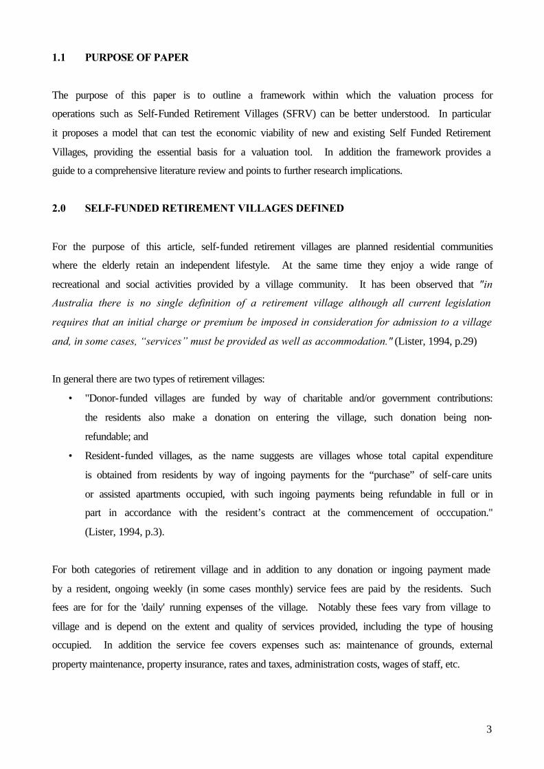
1.1 PURPOSE OF PAPER

The purpose of this paper is to outline a framework within which the valuation process for

operations such as Self-Funded Retirement Villages (SFRV) can be better understood. In particular

it proposes a model that can test the economic viability of new and existing Self Funded Retirement

Villages, providing the essential basis for a valuation tool. In addition the framework provides a

guide to a comprehensive literature review and points to further research implications.

2.0 SELF-FUNDED RETIREMENT VILLAGES DEFINED

For the purpose of this article, self-funded retirement villages are planned residential communities

where the elderly retain an independent lifestyle. At the same time they enjoy a wide range of

recreational and social activities provided by a village community. It has been observed that "in

Australia there is no single definition of a retirement village although all current legislation

requires that an initial charge or premium be imposed in consideration for admission to a village

and, in some cases, “services” must be provided as well as accommodation." (Lister, 1994, p.29)

In general there are two types of retirement villages:

• "Donor-funded villages are funded by way of charitable and/or government contributions:

the residents also make a donation on entering the village, such donation being non-

refundable; and

• Resident-funded villages, as the name suggests are villages whose total capital expenditure

is obtained from residents by way of ingoing payments for the “purchase” of self-care units

or assisted apartments occupied, with such ingoing payments being refundable in full or in

part in accordance with the resident’s contract at the commencement of occcupation."

(Lister, 1994, p.3).

For both categories of retirement village and in addition to any donation or ingoing payment made

by a resident, ongoing weekly (in some cases monthly) service fees are paid by the residents. Such

fees are for for the 'daily' running expenses of the village. Notably these fees vary from village to

village and is depend on the extent and quality of services provided, including the type of housing

occupied. In addition the service fee covers expenses such as: maintenance of grounds, external

property maintenance, property insurance, rates and taxes, administration costs, wages of staff, etc.

4

In general retirement villages can provide a range of accommodation services for the elderly, which

are generally categorized as:

• independent living units

• serviced apartments

• nursing home

3.0 ANALYTICAL FRAMEWORK

The analytical framework as presented in Figure 1 below is proposed as a foundation for valuers

wishing to undertake a valuation of a retirement village. Importantly this framework differentiates

between the tangible and intangible assets of the operation, as well as identifying general value

determinants of the business operation. In particular, the importance of the intangible (Business

Enterprise Value) component is emphasised.

Figure 1 - Framework for Valuation of Self-Funded Retirement Villages

[ Section 4.0 ] [ Section 5.0 ] [ Section 6.0 ] [ Section 7.0 ]

It will be noted that Figure 1 is divided into Sections 4.0, 5.0, 6.0 and 7.0 and are presented below

in this order.

Internal Business Factors

External Business Factors

Value Determinants

Going Concern

Net Operating

Income

Valuation Methodology

Going Concern

Value

Intangible (Business Enterprise

Value)

Tangible Real estate/personal

property

5

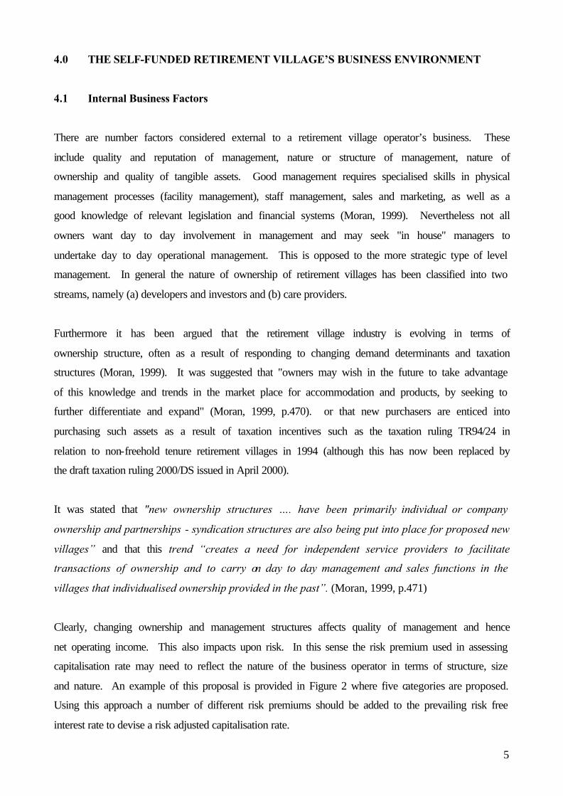
4.0 THE SELF-FUNDED RETIREMENT VILLAGE’S BUSINESS ENVIRONMENT

4.1 Internal Business Factors

There are number factors considered external to a retirement village operator’s business. These

include quality and reputation of management, nature or structure of management, nature of

ownership and quality of tangible assets. Good management requires specialised skills in physical

management processes (facility management), staff management, sales and marketing, as well as a

good knowledge of relevant legislation and financial systems (Moran, 1999). Nevertheless not all

owners want day to day involvement in management and may seek "in house" managers to

undertake day to day operational management. This is opposed to the more strategic type of level

management. In general the nature of ownership of retirement villages has been classified into two

streams, namely (a) developers and investors and (b) care providers.

Furthermore it has been argued that the retirement village industry is evolving in terms of

ownership structure, often as a result of responding to changing demand determinants and taxation

structures (Moran, 1999). It was suggested that "owners may wish in the future to take advantage

of this knowledge and trends in the market place for accommodation and products, by seeking to

further differentiate and expand" (Moran, 1999, p.470). or that new purchasers are enticed into

purchasing such assets as a result of taxation incentives such as the taxation ruling TR94/24 in

relation to non-freehold tenure retirement villages in 1994 (although this has now been replaced by

the draft taxation ruling 2000/DS issued in April 2000).

It was stated that "new ownership structures …. have been primarily individual or company

ownership and partnerships - syndication structures are also being put into place for proposed new

villages” and that this trend “creates a need for independent service providers to facilitate

transactions of ownership and to carry on day to day management and sales functions in the

villages that individualised ownership provided in the past”. (Moran, 1999, p.471)

Clearly, changing ownership and management structures affects quality of management and hence

net operating income. This also impacts upon risk. In this sense the risk premium used in assessing

capitalisation rate may need to reflect the nature of the business operator in terms of structure, size

and nature. An example of this proposal is provided in Figure 2 where five categories are proposed.

Using this approach a number of different risk premiums should be added to the prevailing risk free

interest rate to devise a risk adjusted capitalisation rate.

6

Figure 2 -Risk Premiums (Schilt, 1982)

Apart from the quality of management, the quality of accommodation is a major factor in

determining value and can be narrowed down to three fundamental requirements. Firstly,

accommodation should provide self-care units which enable residents to maintain a comfortable

lifestyle within a homogeneous community in premises that have architectural appeal, coupled with

a practical floor plan. Secondly, hostel or assisted care apartments must be able to provide ongoing

accommodation within the same environment once occupiers of the self-care units are unable to

look after themselves. Finally, there must be facilities withing the retirement village, such as a

community centre, which contributes to the desirability and functional success of any village

(Lister, 1994).

4.2 External Business Factors

Factors external to SFRVs can be described as 'demand drivers' for retirement villages,

incorporating demographic and social factors, the legal and taxation environment and location

linkages. These factors are considered in more detail below.

4.2.1 Demand Drivers

(The following information was derived from research undertaken in 2001 as part of

a ARC SPIRT grant (C79937006) in conjunction with the Retirement Village

Association of Australia and the University of Queensland).

7

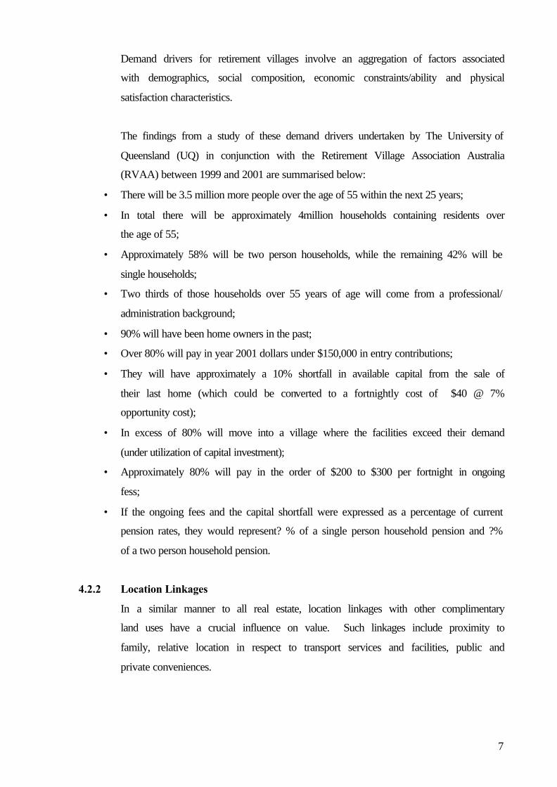
Demand drivers for retirement villages involve an aggregation of factors associated

with demographics, social composition, economic constraints/ability and physical

satisfaction characteristics.

The findings from a study of these demand drivers undertaken by The University of

Queensland (UQ) in conjunction with the Retirement Village Association Australia

(RVAA) between 1999 and 2001 are summarised below:

• There will be 3.5 million more people over the age of 55 within the next 25 years;

• In total there will be approximately 4million households containing residents over

the age of 55;

• Approximately 58% will be two person households, while the remaining 42% will be

single households;

• Two thirds of those households over 55 years of age will come from a professional/

administration background;

• 90% will have been home owners in the past;

• Over 80% will pay in year 2001 dollars under $150,000 in entry contributions;

• They will have approximately a 10% shortfall in available capital from the sale of

their last home (which could be converted to a fortnightly cost of $40 @ 7%

opportunity cost);

• In excess of 80% will move into a village where the facilities exceed their demand

(under utilization of capital investment);

• Approximately 80% will pay in the order of $200 to $300 per fortnight in ongoing

fess;

• If the ongoing fees and the capital shortfall were expressed as a percentage of current

pension rates, they would represent? % of a single person household pension and ?%

of a two person household pension.

4.2.2 Location Linkages

In a similar manner to all real estate, location linkages with other complimentary

land uses have a crucial influence on value. Such linkages include proximity to

family, relative location in respect to transport services and facilities, public and

private conveniences.

8

4.2.3 Legal and Taxation Environment

In recent years the retirement village industry in Australia has been beset by a

number of taxation and legal issues. This had a detrimental effect on the industry.

Major issues included taxation rulings by the Commissioner of Taxation,

introduction of the Goods and Services Tax, Stamp Duty and Practice Directory and

Retirement Villages Act, 1999 (Qld).

5.0 COMPONENTS OF VALUE

As noted from Figure 1, internal and external factors combine to form a number of value

determinants which influence the ‘Going Concern’ value of SFRVs. However, as with all

businesses, SFRVs can be segmented into two value components – tangible and intangible. The

tangible component consists of tangible personal and real property. As already noted the intangible

component is also known as 'Business Enterprise Value'.

Elements of Business Enterprise Value may include:

1. furniture, fixtures and equipment;

2. assembled and trained workforce;

3. name and reputation of management;

4. licences and permits specific to the operator;

5. profit centres i.e. excess of residents' service fees over village operating costs.

6.0 NET OPERATING INCOME

Resident funded retirement villages potentially involve four souces of funds:

• a profit from the initial leasing or selling (receipt of the ingoing contribution) of each

resident unit;

• the value of any undeveloped land;

• the ongoing village-operating profit being the excess of weekly resident service fees over

village-operating costs; and

• the long-term financial entitlements received by the village promoter/manager pursuant to

the executed resident documentation, often referred to Deferred Management Fees

(Hatcher & O'Leary, 1994).

9

7.0 VALUATION METHODOLOGY

In the process of valuing retirement villages it has been proposed that there are two common

approaches for assessing an appropriate discount rate, namely the 'Partitioned Approach' and the

'Comparison to Super Profit Capitalisation Rate' as listed below (Hatcher et.al., 1994).

7.1 Partitioned Approach

Part (a) - Risk Free Rate

Normally represented by the 10 year bond rate, this percentage implicitly considers

inflationary expectations;

Part (b) - Risk Premium Rate

Abitrarily determined and reflects the following categories of risk:

• specialist and entrepreneurial skill of the owner/operator;

• poor marketability and liquidity of the interest;

• security of tenure;

• unfavourable legislative changes;

• possible variation from the assumptions adopted;

• comparison to other forms of investment;

• long-term perceptions of the economy.

7.2 Comparison to "Super Profit" Capitalisation Rate

A relatively common method adopted for the valuation of a business whereby the

perceived net maintainable profit (over and above the standard profit) is capitalised.

Even considering these two approaches, each retirement village would have a different degree of

risk or exposure, requiring a unique capitalisation rate to be applied to each village.

7.3 Asset Management Investment Model (AMM)

Problems associated with the valuation methodology of retirement villages can be summarised as

follows:

• Lack of comparable sale evidence as each SFRV is so different;

• Recognising the role that good business management plays in deriving net income;

• Accounting for the variability of projected cashflows based on varied assumptions and

demographic trends.

10

As a result an argument can be made for the more explicit DCF approach to valuation. However it

can be argued that if such an approach is to applied, then a riguous method is needed with respect to

determining the assumptions upon which cashflows are based. One possible approach was adopted

in the recently completed UQ/RVAA study, where data was collected on present demand drives for

self-funded retirement villages (as discussed earlier in Section 4). This data was then analysed to

develop the Asset Management Investment model presented below. This model was used to test the

risk/return profiles of retirement villages and to measure the investment returns, both before and

after tax. The steps involved in the AMM are outlined below.

Existing Retirement Villages

The first phase of the model identifies existing villages and their asset management

characteristics, such as size, value and vacancies (GIS management).

Population in Catchments

Data is then abstracted on population growth, and potential catchment by social mix and age

(ABS and RVAA) (see Figure 3 and 4)

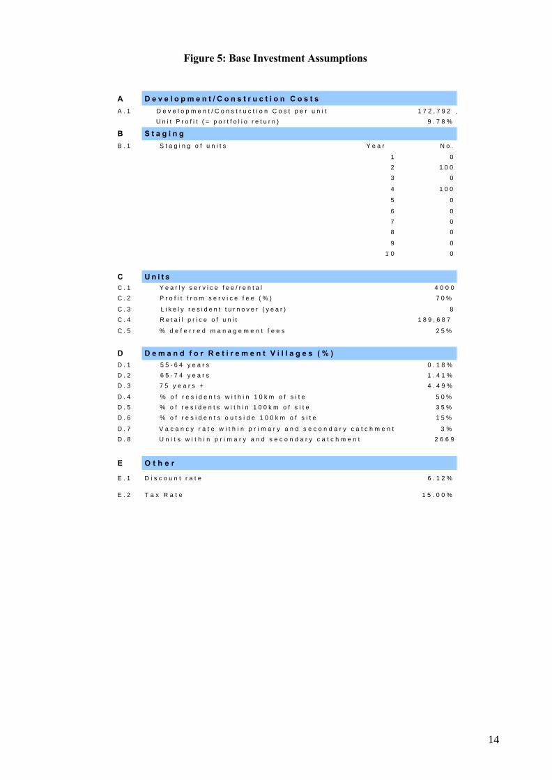
Proposed Village Assumptions

The base investment information section allows for the input of critical assumption such as

(See Figures 5 and 6)

• Staging of the village development by number of units and timing

(assumption entered,

• Development costs (these can be either entered as an assumption or built up

via the development costs worksheet (see Figure 5,

• Entry and exit contributions (assumptions entered),

• On-going management fees (assumptions entered),

• Demand criteria (assumptions fixed based on UQ/RVAA study,

• Taxation rates (assumption entered based on legal structure, example

individual, company or superannuation).

11

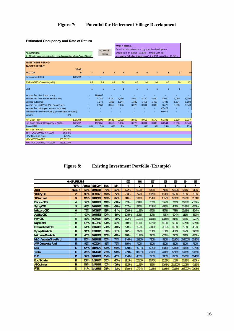
Potential for Retirement Village Development

The model calculates the asset management potential of a village or forecast occupancy

rates of a village over an initial 10 year period using information from the “existing Village”

analysis, “population in Catchments” data and input from the “proposed village

assumptions” section (see Figure 7).

Estimated Pre Taxation Rate of Return (IRR and NPV) (First Iteration)

The model places the information from all of the above sections into an estimated pre-

taxation rate of return cash flow over a 10-year period indicating an initial Internal rate of

Return (IRR)

Portfolio Risk/Return Model

The then requires the development of a portfolio risk return analysis. To undertake this task,

the model requires information on the current investment portfolio of the investment entity,

indicating annual rates of return and weighting on an investment as a percentage of the total

portfolio. From this data the model uses 'portfolio theory' to calculate the portfolio risk and

weighted return (see Figure 8 to 16). The model uses this information to calculate the

investment Beta of the proposed village in relationship to the current investment entities

portfolio. This analysis produces a discount rate that the retirement village cash flow is

required to outperform to enable the investment entities portfolio to continue at the same

risk/return criteria.

Estimated Pre Taxation Rate of Return (IRR and NPV) (Second Iteration)

Following the establishment of discount rate (identified above), the model undertakes a Net

Present Value (NPV) analysis to indicate either a positive or negative result

• Negative result indicating either the entry/exist contribution is require to be

higher or the ongoing management fees require to be increased,

• Positive result is the reverse of the above, e.g. lower entry/exit contribution

or lower ongoing fees.

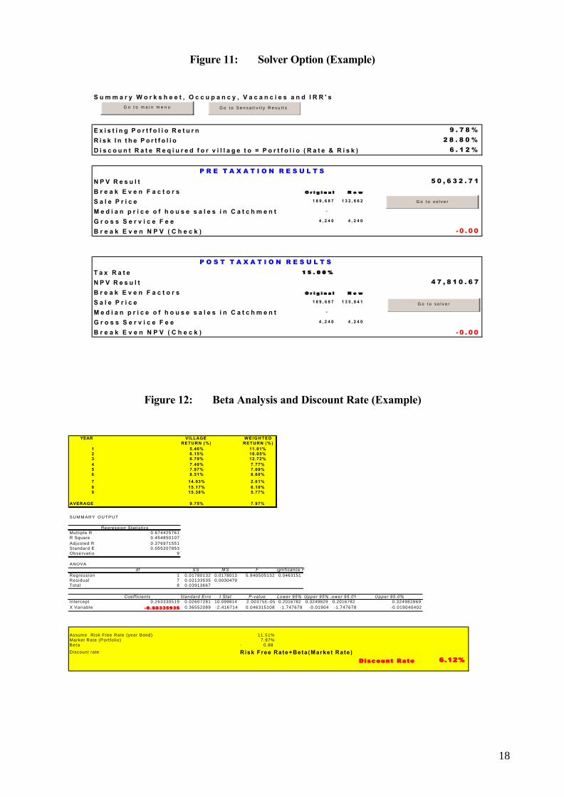
Solver Option

Once the estimated pre taxation rate of return (IRR and NPV) (Second Iteration) is executed

the solver option provides the optimum combination for:

• Entry/exit contributions;

• On-going fees. (See Figure 11)

12

Post Taxation Analysis

The model undertakes a post taxation analysis based on the investment entity nominated in

the “Proposed Village Assumptions” section of the model inclusive of the optimum

combination calculation discussed above (solver option) (See Figure 12)

Sensitivity Option

Finally the model runs an investment sensitivity reviewing occupant and return variations

(see Figure 13).

Note: the example presented below was based on the following assumptions:

• 200 unit village staged over 4 years;

• Land cost per unit of $25,000;

• Initial occupation rate of 85% (based on the demographic model);

• 100% occupataion reached in year 10 (based on the demographic model);

• Competing investment portfolio consisting of:

• 15% cash (short, medium and long term)

• 45% in direct property spread throughout Australia, across commercial and

residential sectors (balanced)

• 20% in Australian Institutional Equities

• 15% overseas equities (Euro SX and FTSE)

• The competing portfolio produced a risk of 28.8% and a weighted return of 9.78%;

• The resulting discount rate needed by the retirement village to provide the same

risk/return profile was 6.12%;

• The impact on the entity contribution was a reduction of 38% (pretaxation) and on the

basis of a company entity 34% (post-taxation).

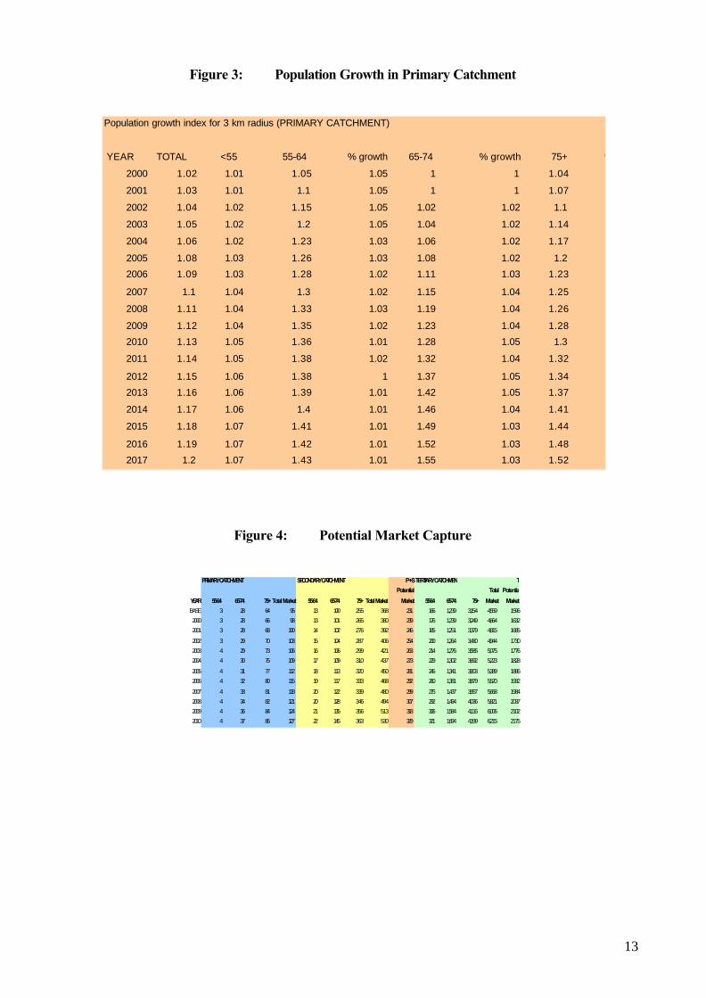
13

Figure 3: Population Growth in Primary Catchment

Population growth index for 3 km radius (PRIMARY CATCHMENT)

YEAR TOTAL <55 55-64 % growth 65-74 % growth 75+ % growth

2000 1.02 1.01 1.05 1.05 1 1 1.04

2001 1.03 1.01 1.1 1.05 1 1 1.07

2002 1.04 1.02 1.15 1.05 1.02 1.02 1.1

2003 1.05 1.02 1.2 1.05 1.04 1.02 1.14

2004 1.06 1.02 1.23 1.03 1.06 1.02 1.17

2005 1.08 1.03 1.26 1.03 1.08 1.02 1.2

2006 1.09 1.03 1.28 1.02 1.11 1.03 1.23

2007 1.1 1.04 1.3 1.02 1.15 1.04 1.25

2008 1.11 1.04 1.33 1.03 1.19 1.04 1.26

2009 1.12 1.04 1.35 1.02 1.23 1.04 1.28

2010 1.13 1.05 1.36 1.01 1.28 1.05 1.3

2011 1.14 1.05 1.38 1.02 1.32 1.04 1.32

2012 1.15 1.06 1.38 1 1.37 1.05 1.34

2013 1.16 1.06 1.39 1.01 1.42 1.05 1.37

2014 1.17 1.06 1.4 1.01 1.46 1.04 1.41

2015 1.18 1.07 1.41 1.01 1.49 1.03 1.44

2016 1.19 1.07 1.42 1.01 1.52 1.03 1.48

2017 1.2 1.07 1.43 1.01 1.55 1.03 1.52

Figure 4: Potential Market Capture

PRIMARY CATCHMENT SECONDARY CATCHMENT P+STERTIARY CATCHMENT T

YEAR 55-64 65-74 75+ Total Market 55-64 65-74 75+ Total Market

Potential

Market 55-64 65-74 75+

Total

Market

Potential

Market

BASE 3 28 64 95 13 100 255 368 231 166 1,239 3,154 4,559 1596

2000 3 28 66 98 13 101 265 380 239 176 1,239 3,249 4,664 1632

2001 3 28 68 100 14 102 276 392 246 185 1,251 3,379 4,815 1685

2002 3 29 70 103 15 104 287 406 254 200 1,264 3,480 4,944 1730

2003 4 29 73 106 16 106 299 421 263 214 1,276 3,585 5,075 1776

2004 4 30 75 109 17 109 310 437 273 229 1,302 3,692 5,223 1828

2005 4 31 77 112 18 113 320 450 281 245 1,341 3,803 5,389 1886

2006 4 32 80 115 19 117 333 468 292 260 1,381 3,879 5,520 1932

2007 4 33 81 118 20 122 339 480 299 275 1,437 3,957 5,668 1984

2008 4 34 82 121 20 128 346 494 307 292 1,494 4,036 5,821 2037

2009 4 36 84 124 21 135 356 513 318 306 1,584 4,116 6,006 2102

2010 4 37 86 127 22 145 363 530 329 321 1,694 4,199 6,215 2175

14

Figure 5: Base Investment Assumptions

A D e v e l o p m e n t / C o n s t r u c t i o n C o s t s

A . 1 D e v e l o p m e n t / C o n s t r u c t i o n C o s t p e r u n i t 1 7 2 , 7 9 2

U n i t P r o f i t ( = p o r t f o l i o r e t u r n ) 9 . 7 8 %

B S t a g i n g

B . 1 S t a g i n g o f u n i t s Y e a r N o .

1 0

2 1 0 0

3 0

4 1 0 0

5 0

6 0

7 0

8 0

9 0

1 0 0

C U n i t sC . 1 Y e a r l y s e r v i c e f e e / r e n t a l 4 0 0 0

C . 2 P r o f i t f r o m s e r v i c e f e e ( % ) 7 0 %

C . 3 L i k e l y r e s i d e n t t u r n o v e r ( y e a r ) 8

C . 4 R e t a i l p r i c e o f u n i t 1 8 9 , 6 8 7

C . 5 % d e f e r r e d m a n a g e m e n t f e e s 2 5 %

D D e m a n d f o r R e t i r e m e n t V i l l a g e s ( % )D . 1 5 5 - 6 4 y e a r s 0 . 1 8 %

D . 2 6 5 - 7 4 y e a r s 1 . 4 1 %

D . 3 7 5 y e a r s + 4 . 4 9 %

D . 4 % o f r e s i d e n t s w i t h i n 1 0 k m o f s i t e 5 0 %

D . 5 % o f r e s i d e n t s w i t h i n 1 0 0 k m o f s i t e 3 5 %

D . 6 % o f r e s i d e n t s o u t s i d e 1 0 0 k m o f s i t e 1 5 %

D . 7 V a c a n c y r a t e w i t h i n p r i m a r y a n d s e c o n d a r y c a t c h m e n t 3 %

D . 8 U n i t s w i t h i n p r i m a r y a n d s e c o n d a r y c a t c h m e n t 2 6 6 9

E O t h e r

E . 1 D i s c o u n t r a t e 6 . 1 2 %

E . 2 T a x R a t e 1 5 . 0 0 %

15

Figure 6: Development Costs

PRELIMINARY DEVELOPMENT COSTSPRELIMINARY DEVELOPMENT COSTS

No. Units 30 Note: Note: Blue figures are automatically calculatedI Bed 2 You are only required to fill in the black figures2 bed 23

3 bed 34 bed 2No. Bed 65Avg Beds/unit 2.1666667 30

Rate/ Unit Rate Roomland Purchaseland Purchase 2,000,000 Stamp Duty 80,000 Valuation Fees 30,000 2,110,000 70,333 32,461.54

ConstructionNo. Area (m2) Rate $/m2 Cost

I Bed 2 35 650 45,500 2 bed 23 60 650 897,000 3 bed 3 90 600 162,000 4 bed 2 110 550 121,000 Central facilities 1 400 900 360,000 Bowling Green 1 1,800 50 90,000 Tennis Court 2 900 40 72,000 Other - car parking 50 25 50 62,500 Total area of land use 7,190 Total land area 12,000 Landscape 1 4,810 50 240,500 TOTAL BUILDING COST 2,050,500 Design & PM 8.00% 164,040 TOTAL D&C 2,214,540 73,818 34,070

Marketing & Approval Costs

DA 2,215 BA 17,975 Headworks 65 1 5,000 325,000 Marketing 1 4.00% 227,624 572,814 19,094 8,812.52

Development Finance 6.12%

Constrcution period (Mths) 4Pre Constrcution period (Mths) 12Development Period 16

Land 172,299 Construction 81,376 Marketing & Approvals 32,742 286,417 9,547 4,406

TOTAL DEVELOPMENT COSTS 5,183,771 172,792 79,750

Development Profit 9.78% 506,839 16,895 7,798

TOTAL DEVELOPMENT INCOME 5,690,609 189,687 87,548

16

Figure 7: Potential for Retirement Village Development

Estimated Occupancy and Rate of ReturnWhat it Means…

Based on all costs entered by you, the development

Assumptions should yield an IRR of 15.38% If there was full 1. All factors are pre-calculated based on numbers from "Input Sheet" occupancy (all other things equal), the IRR would be 15.84%

INVESTMENT PERIOD

TARGET RESULTYEAR

FACTOR 0 1 2 3 4 5 6 7 8 9 10

Development Cost 172,792 - -

ESTIMATED Occupancy (%) 85 84 87 86 89 91 94 96 99 103

Unit 1 1 1 1 1 1 1 1 1 1

Income Per Unit (Lump sum) - 189,687 - - - - - - - - Income Per Unit (Gross service fee) - 4,240 4,360 4,480 4,600 4,720 4,840 4,960 5,080 5,200 Service outgoings - 1,272 1,308 1,344 1,380 1,416 1,452 1,488 1,524 1,560 Income Per Unit/Profit (Net service fee) - 2,968 3,052 3,136 3,220 3,304 3,388 3,472 3,556 3,640 Income Per Unit (upon resident turnover) - - - - - - - 47,422 - - Escalated Income Per Unit (upon resident turnover) - - - - - - - 60,072 - -

Inflation 3%

Net Cash Flow 172,792- - 192,190 2,645 2,702 2,862 3,013 3,172 61,101 3,530 3,737 Net Cash Flow if Occupancy = 100% 172,792- - 192,655 3,052 3,136 3,220 3,304 3,388 63,544 3,556 3,640 Annual IRR -100% 0% 5% 6% 7% 7% 8% 9% 15% 15% 15%IRR - ESTIMATED 15.38%IRR - OCCUPANCY = 100% 15.84%NPV Discount Rate 6.12%NPV - ESTIMATED $50,632.71NPV - OCCUPANCY = 100% $53,821.86

Go to main

menu

Figure 8: Existing Investment Portfolio (Example)

ANNUAL RETURNS 1999 1998 1997 1996 1995 1994 1993

YEAR Average Std. Dev Max. Min. 1 2 3 4 5 6 730 Bill ASSET 1 5.8% 0.0106141 7.6% 5.0% 5.12% 5.02% 5.45% 7.17% 7.5800% 5.41% 5.18%180 Day Bill 2 9.0% 0.014667 11.4% 7.7% 7.74% 7.77% 10.21% 11.38% 9.75% 7.96% 7.98%10 Year Bond 3 11.5% 0.0207331 14.3% 8.7% 8.65% 9.14% 11.49% 13.57% 14.28% 11.67% 11.74%Brisbane CBD 4 5.9% 0.0533859 11.0% -5.6% 7.19% 8.11% 7.64% 5.77% 7.44% 11.01% -5.63%Sydney CBD 5 6.1% 0.0698936 11.9% -8.6% 7.17% 9.25% 11.51% 6.78% 4.42% 11.88% -8.60%Melbourne CBD 6 7.2% 0.0722057 13.9% -8.1% 10.00% 11.11% 9.76% 5.67% 7.78% 13.92% -8.14%Adelaide CBD 7 -0.3% 0.0658408 10.4% -8.6% 10.40% 2.98% 3.07% -4.68% -6.04% 1.11% -8.63%Perth CBD 8 8.3% 0.084698 16.0% -9.8% 9.12% 11.38% 16.04% 13.98% 8.14% 9.55% -9.77%Major Retail 9 10.1% 0.029815 12.8% 5.3% 9.99% 5.34% 12.71% 6.99% 9.90% 12.76% 12.76%Brisbane Residential 10 5.4% 0.1058422 29.0% -1.8% 1.49% 1.22% 29.00% -1.83% 0.93% 2.25% 4.89%Sydney Residential 11 9.1% 0.1288917 38.0% 1.8% 6.62% 7.47% 2.61% 1.81% 4.31% 3.22% 38.00%Melbourne Residential 12 4.0% 0.0491329 11.3% -1.8% 9.86% 11.29% 3.75% -0.31% 2.76% 2.21% -1.83%MLC - Australian Share Fund 13 11.3% 0.0284128 15.3% 7.1% 14.40% 15.30% 7.10% 9.30% 11.50% 10.9000% 10.30%AMP Conservative Fund 14 8.3% 0.006264 8.9% 7.3% 8.80% 7.60% 8.90% 8.20% 8.30% 8.80% 7.30%

NAB 15 17.1% 0.0070576 17.9% 15.9% 17.90% 15.90% 17.70% 16.80% 17.00% 16.80% 17.70%Telstra 16 21.9% 0.0545143 29.9% 17.0% 29.90% 28.70% 20.10% 22.80% 17.90% 17.00% 17.00%BHP 17 9.4% 0.0340329 15.4% 4.5% 15.40% 4.50% 7.20% 9.10% 8.40% 11.00% 10.40%Euro SX Index 18 16.6% 0.1203107 31.2% -1.3% 31.15% 22.86% 16.76% 21.22% 1.68% 23.82% -1.33%All Ordinaries 19 11.6% 0.1563594 40.3% -12.0% 13.25% 11.23% 3.22% 10.08% 15.1600% -12.01% 40.26%FTSE 20 14.1% 0.1124592 21.8% -10.3% 17.80% 17.24% 21.83% 11.66% 20.32% -10.3000% 20.06%

17

Figure 9: Portfolio Weighting (Example)

Figure 10: Portfolio Analysis (Example)

COVARIANCE MATRIX (ASSET * WEIGHTING)

ASSET 1 2 3 4 5 6 7 8 9 10 11 12 13 14 15 161 0.002500 0.001883 0.002149 0.000331 0.000015- 0.000001- 0.001349- 0.000581 0.000582- 0.000692- 0.000881- 0.001068- 0.000739- 0.000184 0.000371- 0.000796- 2 0.001883 0.002500 0.001791 0.000269 0.000433 0.000008 0.000912- 0.001177 0.000370- 0.000587 0.001036- 0.001159- 0.001709- 0.000550 0.000043 0.000593-

3 0.002149 0.001791 0.002500 0.000256- 0.000470- 0.000594- 0.001986- 0.000059- 0.000379 0.000138- 0.000179- 0.001962- 0.001565- 0.000045- 0.000074- 0.001847- 4 0.000331 0.000269 0.000256- 0.002500 0.002391 0.002475 0.001445 0.002166 0.000605- 0.000078 0.002348- 0.001270 0.000428 0.001775 0.001012- 0.000678

5 0.000015- 0.000433 0.000470- 0.002391 0.002500 0.002406 0.001605 0.002319 0.000530- 0.000576 0.002306- 0.001242 0.000081 0.001817 0.000867- 0.000780 6 0.000001- 0.000008 0.000594- 0.002475 0.002406 0.002500 0.001683 0.002119 0.000591- 0.000154 0.002258- 0.001498 0.000597 0.001754 0.000959- 0.000878 7 0.001349- 0.000912- 0.001986- 0.001445 0.001605 0.001683 0.002500 0.001295 0.000247- 0.000485 0.001195- 0.002033 0.001059 0.001471 0.000279 0.001797

8 0.000581 0.001177 0.000059- 0.002166 0.002319 0.002119 0.001295 0.002500 0.000939- 0.000611 0.002395- 0.001043 0.000198- 0.001652 0.000788- 0.000918 9 0.000582- 0.000370- 0.000379 0.000605- 0.000530- 0.000591- 0.000247- 0.000939- 0.002500 0.001262 0.000824 0.001212- 0.001372- 0.000852 0.001771 0.001692- 10 0.000692- 0.000587 0.000138- 0.000078 0.000576 0.000154 0.000485 0.000611 0.001262 0.002500 0.000179- 0.000112- 0.001560- 0.000930 0.001077 0.000526-

11 0.000881- 0.001036- 0.000179- 0.002348- 0.002306- 0.002258- 0.001195- 0.002395- 0.000824 0.000179- 0.002500 0.000957- 0.000002 0.001811- 0.000817 0.000708- 12 0.001068- 0.001159- 0.001962- 0.001270 0.001242 0.001498 0.002033 0.001043 0.001212- 0.000112- 0.000957- 0.002500 0.001889 0.000411 0.000691- 0.002105

13 0.000739- 0.001709- 0.001565- 0.000428 0.000081 0.000597 0.001059 0.000198- 0.001372- 0.001560- 0.000002 0.001889 0.002500 0.000650- 0.000984- 0.001717 14 0.000184 0.000550 0.000045- 0.001775 0.001817 0.001754 0.001471 0.001652 0.000852 0.000930 0.001811- 0.000411 0.000650- 0.002500 0.000832 0.000064 15 0.000371- 0.000043 0.000074- 0.001012- 0.000867- 0.000959- 0.000279 0.000788- 0.001771 0.001077 0.000817 0.000691- 0.000984- 0.000832 0.002500 0.000453-

16 0.000796- 0.000593- 0.001847- 0.000678 0.000780 0.000878 0.001797 0.000918 0.001692- 0.000526- 0.000708- 0.002105 0.001717 0.000064 0.000453- 0.002500 17 0.000338- 0.000696- 0.000496- 0.000270- 0.000436- 0.000215- 0.000775 0.000648- 0.001026 0.000622- 0.000321 0.000154- 0.000302 0.000967 0.001677 0.000216

18 0.000873- 0.000360- 0.001524- 0.001641 0.001832 0.001791 0.002113 0.001611 0.000823- 0.000195- 0.001532- 0.001558 0.000881 0.001331 0.000422- 0.001747 19 0.000055- 0.000316- 0.000075 0.002290- 0.002324- 0.002259- 0.001205- 0.001955- 0.000025- 0.000372- 0.002092 0.000616- 0.000219 0.001883- 0.000797 0.000071- 20 0.000205 0.000479 0.000152- 0.001099- 0.000981- 0.001055- 0.000186- 0.000352- 0.000471- 0.000765 0.000688 0.000410 0.000019 0.000806- 0.000779 0.000682

Variances 0.002500 0.002500 0.002500 0.002500 0.002500 0.002500 0.002500 0.002500 0.002500 0.002500 0.002500 0.002500 0.002500 0.002500 0.002500 0.002500 Co-

Variances 0.002428- 0.000070 0.006952- 0.007069 0.007553 0.007432 0.008959 0.008157 0.003347- 0.002126 0.013042- 0.005528 0.001585- 0.009393 0.001452 0.004894

A S S E T 1 W e i g h t i n g3 0 B i l l 1 5 . 0 0 %1 8 0 D a y B i l l 2 5 . 0 0 %1 0 Y e a r B o n d 3 5 . 0 0 %B r i s b a n e C B D 4 5 . 0 0 %S y d n e y C B D 5 5 . 0 0 %

M e l b o u r n e C B D 6 5 . 0 0 %A d e l a i d e C B D 7 5 . 0 0 %P e r t h C B D 8 5 . 0 0 %M a j o r R e t a i l 9 5 . 0 0 %

B r i s b a n e R e s i d e n t i a l 1 0 5 . 0 0 %

S y d n e y R e s i d e n t i a l 1 1 5 . 0 0 %

M e l b o u r n e R e s i d e n t i a l 1 2 5 . 0 0 %M L C - A u s t r a l i a n S h a r e F u n d 1 3 5 . 0 0 %A M P C o n s e r v a t i v e F u n d 1 4 5 . 0 0 %N A B 1 5 5 . 0 0 %T e l s t r a 1 6 5 . 0 0 %B H P 1 7 5 . 0 0 %E u r o S X I n d e x 1 8 5 . 0 0 %A l l O r d i n a r i e s 1 9 5 . 0 0 %F T S E 2 0 5 . 0 0 %

T O T A L 1 0 0 . 0 0 %

18

Figure 11: Solver Option (Example)

S u m m a r y W o r k s h e e t , O c c u p a n c y , V a c a n c i e s a n d I R R ' s

E x i s t i n g P o r t f o l i o R e t u r n 9 . 7 8 %R i s k I n t h e P o r t f o l i o 2 8 . 8 0 %D i s c o u n t R a t e R e q i u r e d f o r v i l l a g e t o = P o r t f o l i o ( R a t e & R i s k ) 6 . 1 2 %

P R E T A X A T I O N R E S U L T SN P V R e s u l t 5 0 , 6 3 2 . 7 1B r e a k E v e n F a c t o r s O r i g i n a lO r i g i n a l N e wN e w

S a l e P r i c e 1 8 9 , 6 8 7 1 3 2 , 6 6 2

M e d i a n p r i c e o f h o u s e s a l e s i n C a t c h m e n t -

G r o s s S e r v i c e F e e 4 , 2 4 0 4 , 2 4 0

B r e a k E v e n N P V ( C h e c k ) - 0 . 0 0

P O S T T A X A T I O N R E S U L T ST a x R a t e 1 5 . 0 0 %1 5 . 0 0 %

N P V R e s u l t 4 7 , 8 1 0 . 6 7B r e a k E v e n F a c t o r s O r i g i n a lO r i g i n a l N e wN e w

S a l e P r i c e 1 8 9 , 6 8 7 1 3 5 , 8 4 1

M e d i a n p r i c e o f h o u s e s a l e s i n C a t c h m e n t -

G r o s s S e r v i c e F e e 4 , 2 4 0 4 , 2 4 0

B r e a k E v e n N P V ( C h e c k ) - 0 . 0 0

G o t o m a i n m e n u G o t o S e n s a t i v i t y R e s u l t s

G o t o s o l v e r

G o t o s o l v e r

Figure 12: Beta Analysis and Discount Rate (Example)

YEAR VILLAGE WEIGHTEDRETURN (%) RETURN (%)

1 5.46% 11.01%2 6.15% 10.05%3 6.79% 12.72%4 7.40% 7.77%5 7.97% 7.09%6 8.51% 8.60%

7 14.93% 2.61%8 15.17% 6.10%9 15.38% 5.77%

AVERAGE 9.75% 7.97%

SUMMARY OUTPUT

Regression Statist icsMult iple R 0.674425761R Square 0.454850107Adjusted R Square 0.376971551Standard Error 0.055207853Observat ions 9

ANOVAdf S S M S F Significance F

Regression 1 0.01780132 0.0178013 5.840505132 0.0463151Residual 7 0.02133535 0.0030479Total 8 0.03913667

Coefficients Standard Error t Stat P-value Lower 95% Upper 95%Lower 95.0% Upper 95.0%Intercept 0.263330519 0.02607281 10.099814 2.00375E-05 0.2016782 0.3249829 0.2016782 0.324982869X Variable 1 - 0 .88335935-0 .88335935 0.36552089 -2.416714 0.046315108 -1.747678 -0.01904 -1.747678 -0.019040402

Assume Risk Free Rate (year Bond) 11.51%Market Rate (Port fol io) 7.97%Beta 0.88-

Discount rate Risk Free Rate+Beta (Market Rate )

Discount Ra teD iscount Ra te 6 .12%6.12%

19

Figure 13: Village Sensitivity Analysis (Example)

Estimated over/under supply of units within primary and secondary catchment: with and without development

Without Development With Development

Estimated Occupancy (%)

Estimated Vacancies (No. units)

Estimated Occupancy

(%)

Estimated Vacancies (No. units)

Year 1 85 397 85 3972 87 334 84 4343 90 269 87 3694 93 197 86 3975 96 119 89 3196 98 53 91 2537 101 -17 94 1838 103 -90 96 1109 107 -179 99 21

10 110 -277 103 -77

Scenarios Results Interpretation1. Estimated IRR 15.38% Based on available data, the development can expect an IRR of 15.38%2. IRR if Occupancy = 100% 15.84% All other things being equal, if occupancy = 100%, the return would equal 15.84%3. Required Occupancy if IRR = 5% 72% If occupancy averaged at 72% then the IRR would equal 5%4. Required Occupancy if IRR = 20% 107% If occupancy averaged at 107% then the IRR would equal 20%5. Required Occupancy if IRR = 30% 131% If occupancy averaged at 131% then the IRR would equal 30%6. Dev cost if IRR = 5% 192,060$ If the development cost for one unit equalled $192,060 then the IRR would equal 5%7. Dev cost if IRR = 20% 128,433$ If the development cost for one unit equalled $128,433 then the IRR would equal 20%8. Dev cost if IRR = 30% 104,368$ If the development cost for one unit equalled $104,368 then the IRR would equal 30%

Do NOT use these results until you have used the solver on each of the worksheets relating to the scenarios If you modify any variables on the "Input Sheet" you will need to 'resolve' these worksheets again.

-400

-300

-200

-100

0

100

200

300

400

500

1 2 3 4 5 6 7 8 9 10

Und

er (-

)/ O

ver (

+) S

uppl

y of

Uni

ts

Without Development With Development

Over Supply

Under Supply

8.0 CONCLUSION

Although the AMM outlined above is based on the viability of a new development it can be adapted

to provide a typical 'if what' spreadsheet analysis of an existing SFRV. In particular, with

increasing interest from institutional investors in this sector it makes sense for valuation analysis to

incorporate the effects of including retirement village assets in portfolio return and risk.

The AMM has the capacity to factor in both internal and external business factors of a retirement

village operation. As stated by Hatcher et.al. (1994) the most difficult portion of the valuation of

SFRVs is the valuation of long-term entitlements from deferred management fees and rolloover

contracts. There is no one general accepted approach with respect to determining the variables

upon which this portion of cashflow is based. It is proposed the AMM could provide the standard.

20

REFERENCE LIST (Peter, please write in details)

Hatcher, J. & O'Leary, J., (1994), 'Valuing Retirement Villages' in The Valuer and Land Economist,

Vol.33, No.1, pp.34-46

Kinard, J., (2001) (page 8)

Lennhoffs, D.C., (1999). (page 2)

Lister, (1994) (page 3)

Moran, (1999) (page 5)

Schilt, J.H., (1982), 'A Rational Approach to Capitalisation Rates for Discounting the Future

Income Stream of a Closely Held Company' in The Financial Planner, January, p.20.