Synchrotron Research Institute

German-Armenian Joint Practical Course on Accelerator Physics

Electron Beam Parameter Measurements

Supervisor: Dr. Artsrun Sargsyan

YEREVAN, ARMENIA 2019

Supported by the German Federal Foreign Office under Kapitel 0504, Titel 68713

Contents

1. Introduction ......................................................................................... 3

1.1 Why do we need particle accelerators? ............................................................. 3

1.2 Forces to accelerate particles............................................................................ 4

1.3 Overview of the accelerators development ....................................................... 6

2. Linear beam optics ............................................................................ 11

2.1 Charged Particle motion in magnetic field ....................................................... 12

2.2 Accelerator magnets ....................................................................................... 13

2.2.1. Dipole magnet .......................................................................................... 14

2.2.2. Quadrupole magnet ................................................................................. 15

2.2.3 Solenoid magnet ....................................................................................... 17

2.3 Transformation Matrices .................................................................................. 18

2.3.1. Drift space ................................................................................................ 20

2.3.2. Dipole sector magnet ............................................................................... 20

2.3.3. Quadrupole magnet ................................................................................. 20

2.3.4. Solenoid magnet ...................................................................................... 21

3. Phase Space ellipse, emittance and Twiss parameters ..................... 23

3.1. Transformation of the beta function ................................................ 26

3.2. The Beam matrix ............................................................................ 27

3.3 FODO structure ............................................................................................... 28

4. Electron Beam Parameter Measurements at AREAL Linac ............... 29

4.1. Introduction..................................................................................................... 29

4.2. Beam energy and energy spread measurements........................................... 33

4.2.1. Electron beam energy and energy spread measurement control tools .... 34

4.2.2. Measurement tasks .................................................................................. 37

4.2.3 Measurement procedure ........................................................................... 38

4.3. Beam Transverse Emittance Measurements.................................................. 39

4.3.1. Solenoid/Quadrupole scan technique ...................................................... 40

4.3.2. Emittance determination errors ................................................................ 42

4.3.3. Emittance measurement tool ................................................................... 43

4.3.4. Measurement tasks .................................................................................. 45

4.3.5. Measurement procedure .......................................................................... 45

Bibliography .......................................................................................... 46

1

2

1. Introduction

The present chapter 1 provides an overview of various accelerator principles as a

background of the essentials of this course. The less interested students may skip

this chapter (which would be certainly a pity!) and start with chapter 2 right away.

1.1 Why do we need particle accelerators?

In contemporary scientific research, the structure of various natural and man-made

objects, their basic building blocks and the interaction between these blocks and

structures are of great interest. Taking an atomic scale motion picture of a chemical

process or unraveling the complex molecular structure of a single protein or virus are

the new existing experiments. In Fig. 1.1 the characteristic sizes and times for

various structures and processes are shown. The structures usually have

extraordinarily small sizes, sometimes well below 10−15𝑚, and the time of some

processes about a few femtoseconds (1 fs = 10−15 sec).

Figure 1.1. The characteristic sizes and times for various structures and processes.

The microblocs/microparticles and ultrafast processes in a matter can be studied by

means of ultrashort beams of electromagnetic radiation and/or high energy charged

particles. The wavelength of the electromagnetic radiation must be small compared

to the size of a structure.

The photon energy 𝐸𝛾 for the wavelength 𝜆 = 10−15𝑚 is

𝐸𝛾 = ℎ𝜐 = ℎ𝑐𝜆

= 2 ∗ 10−10𝐽. (1.1)

3

Such high energy photon beams are usually generated by accelerated/decelerated

charged particles having energy 𝐸𝑒 greater than 𝐸𝛾. The conventional method of

obtaining high energy charged particles is based on the interaction with high electric

fields. In particular, to obtain electron beams being able to generate photons with

energy given in (1.1), they should be passed through the potential difference

𝑈 > 1.2 ∗ 109𝑉 (𝐸𝑒 = 𝑒𝑈).

If investigations in matter are carried out directly with particle beams, then the length

of the particle De Broglie wave should be smaller than the characteristic sizes of the

system.

𝜆𝐵 = ℎ𝑝

= ℎ𝑐𝐸

, (1.2)

where 𝑝 and 𝐸 are the momentum and energy of particles.

In the SI system the unit for measuring an energy is J (Joule), but in high energy

physics the eV (electron volt) units are more suitable. 1eV is the kinetic energy

gained by a particle of elementary charge 𝑒 = 1.602 × 10−19𝐶 as it crosses a

potential difference of ∆𝑈 = 1𝑉. The conversion factor thus is 1𝑒𝑉 = 1.602 × 10−19𝐽 .

Another important application of high energy charged particles is the production of

new heavy elementary particles via beam-beam collision. The amount of energy

needed to produce new particles should be greater than the sum of rest energies of

produced particles. Recall that the rest energy of a particle is defined by the

fundamental relation

𝐸 = 𝑚0𝑐2, (1.3)

where 𝑚0 is the rest mass of the particle.

1.2 Forces to accelerate particles

In the first part it was shown that the high energy particle beams are important tools

in nowadays research. Accelerators are the devices which accelerate the charged

particle beams. Since the velocity of high energy particles is close to the speed of

light (𝑐 = 3 ∗ 108𝑚/𝑠), the energy must be considered in the relativistic form

𝐸 = �𝑚02𝑐4 + 𝑝2𝑐2 (1.4)

4

Here 𝑚0 is the rest mass and 𝑝 is the momentum of the particle. The relativistic

particle momentum is given by the relation 𝑝 = 𝛾𝑚0𝑐, where 𝛾 = �1 − 𝛽2 is the

Lorentz factor and 𝛽 = 𝑣𝑐. The only free variable in Eq. (1.4) is the momentum 𝑝 and,

therefore, to increase the energy we should increase the momentum 𝑝.

According to the Newton’s second law the only way to change the momentum 𝑝 of

the particle is to act by a force 𝐹

�̇� = 𝑭 (1.5)

In order to reach high kinetic energies, sufficiently strong force must be acted on

the particle on sufficient period of time.

In nature we have four types of interactions: strong, weak, gravity and

electromagnetic. For strong and weak forces the action range is below 10−15𝑚 and

therefore these forces are not usable for acceleration of the particles. Gravity is

many orders of magnitude weaker. The only possible option is to use

electromagnetic forces. On a charged particle with velocity 𝑣 and charge 𝑞, the

electromagnetic field with the magnetic component 𝑩 and electric component 𝑬 acts

by the Lorentz force

𝐹𝑙 = 𝑞(𝒗 × 𝑩 + 𝑬) (1.6)

As the particle moves from some position 𝒓𝟏 to 𝒓𝟐, its energy changes by the amount

∆𝐸 = ∫ 𝑭𝑑𝒓𝒓𝟐𝒓𝟏

= 𝑞 ∫ (𝒗 × 𝑩 + 𝑬)𝑑𝒓𝒓𝟐𝒓𝟏

. (1.7)

During the motion the path element 𝑑𝒓 is always parallel to the velocity vector 𝒗. The

vector 𝒗 × 𝑩 is thus perpendicular to 𝑑𝒓, i.e. (𝒗 × 𝑩) ∙ 𝒅𝒓 = 𝟎. Hence the magnetic

field 𝑩 does not change the energy of the particle. An increase in energy can thus

only be achieved by the use of electric fields. The gain in energy directly follows by

Eq. (1.7) and is

∆𝐸 = ∫ 𝑬𝑑𝒓 = 𝑒𝑈𝒓𝟐𝒓𝟏

(1.8)

where 𝑈 is the voltage crossed by the particle.

Although the magnetic field does not contribute to the energy of the particle, it is

required to steer, bend and focus charged particle beams.

5

The main tasks in accelerator physics are the acceleration and steering of charged

particle beams. Both processes rely on the interaction with electromagnetic forces

and hence on the foundations of the classical electrodynamics. Here Maxwell’s

equations are of fundamental importance [1].

1.3 Overview of the accelerators development

Since 1920s various machines were built to accelerate the charged particle beams

for experimental physics, always with the principal objective of reaching ever higher

energies.

The simplest particle accelerators use a constant electric field between to electrodes,

produced by a high voltage generator. This principle is illustrated in Fig 1.2. One of

the electrodes represents the particle source. In case of electron beams this is a

thermionic cathode. Protons as well as light and heavy ions, are extracted from the

gas phase by using a further DC or high frequency voltage to ionize a very rarified

gas and so produce a plasma inside the particle source. Charged particles are then

continuously emitted from the plasma, and are accelerated by the electric field. In the

accelerating region there is a relatively good vacuum, in order to avoid collision with

residual gas molecules. The particles are thus continuously accelerated without any

loss of energy until they reach the second electrode. There they exit the accelerator

and usually traverse a further field-free drift region, through which they travel at

constant energy until they reach the target. This principle is very widely employed in

research and technology. The particle energies which can be reached by this

method, however, is very limited. In electrostatic accelerator the maximum

achievable energy is directly proportional to the maximum voltage which can be

developed, and this gives the energy limit. At higher voltages the field strength closer

to electrodes grows so much that ions and electrons produced in this region are

accelerated to considerable energies. They collide with residual gas molecules and

so produce many more ions, which themselves undergo the same processes. The

result is an avalanche of charge carriers causing spark discharge and the break-

down of high voltage. This process, called corona formation, limits the maximum

achievable energy.

6

Figure 1.2. General principle of electrostatic accelerator.

In order to avoid this problem the Swede Ising in 1925 suggested to use rapidly

changing high frequency voltages instead of direct voltages. Three years later

Wideroe performed the first successful test of a linear accelerator based on this

principle (Fig. 1.3). It consists of a series of metal drift tubes arranged along the

beam axis connected with alternating polarity, to a radiofrequency supply, which

delivers a voltage of the form 𝑈(𝑡) = 𝑈𝑚𝑎𝑥𝑆𝑖𝑛(𝜔𝑡). During a half period the voltage

applied to the first drift tube acts to accelerate the particles leaving the ion source.

The particles reach the first drift tube with a velocity 𝑣1. They then pass through this

drift tube which shields them from external fields. Meanwhile the direction of the RF

field is reversed. When they reach the gap between the first and second drift tubes,

they again undergo acceleration. This process is repeated for each of the drift tubes.

After the 𝒾-th drift tube the particles of charge 𝑞 have reached an energy

𝐸𝑖 = 𝑖𝑞𝑈𝑚𝑎𝑥𝑆𝑖𝑛(Ψ0) (1.9)

where Ψ0 is the average phase of the RF voltage that the particles see as they cross

the gaps. It is evident that the energy is again proportional to the number of stages 𝒾

traversed by the particles. The important point, however, is that the largest voltage in

the entire system is never greater then 𝑈𝑚𝑎𝑥. It is therefore possible, in principle, to

produce arbitrarily high particle energies without encountering the problem of voltage

discharge. This is the decisive advantage of RF accelerators over the electrostatic

systems. For this reason almost all particle accelerators nowadays use high-

frequency alternating voltages, produced by powerful RF supplies.

7

Figure 1.3. Wideroe linear accelerator

Although linear accelerators can in principle reach arbitrarily high particle energies,

the length and hence the cost of the machine grows with energy. It is therefore

desirable to drive the particles around a circular path and so use the same

accelerating structure many times. The first circular accelerator to be developed

according to this principle was the cyclotron, proposed by E.O. Lawrence at the

University of California in 1930. A year later Livingston succeeded in experimentally

demonstrating the operation of such a machine. In 1932 they together built the first

proton cyclotron suitable for experiments, with a peak energy of 1.2𝑀𝑒𝑉.

To make the particles follow a circular path the cyclotron uses an iron magnet which

produces a homogeneous magnetic field 𝐵𝑧 between its two round poles (Fig. 1.4).

The particles circulate in a plane between the poles with a revolution frequency

𝜔𝑧 = 𝑞𝑚𝐵𝑧 (1.10)

which is also known as the cyclotron frequency.

8

Figure 1.4. The scheme of cyclotron.

Notice that the cyclotron frequency does not depend on the particle velocity at all.

This is because of the fact that as the momentum increases, the orbit radius and,

hence, the circumference along which the particles travel increase in proportion,

provided that the mass 𝑚 remains constant. This condition is of course only satisfied

for non-relativistic particles.

Classical cyclotrons can accelerate protons, deuterons, and alpha particles up to

about 22MeV per elementary charge. At these energies the motion is still sufficiently

non-relativistic. At higher energies the cyclotron frequency decreases inversely

proportional to the increasing particle mass 𝑚(𝐸). If the frequency of the RF supply

is decreased accordingly, much higher energies can be reached. This principle is

employed in the synchrocyclotron.

A more effective method is adopted in the isochroncyclotron, in which the magnetic

field is increased in such a way that the cyclotron frequency remains constant,

namely

𝜔𝑧 = 𝑒 𝐵𝑧(𝐸)𝑚(𝐸) = 𝐶𝑜𝑛𝑠𝑡 (1.11)

However, this approach is problematic because the beam becomes defocused by the

changing magnetic field. To resolve this issue, isochroncyclotrons use magnets with

rather complex pole shapes, which compensate this loss of focusing with so-called

“edge-focusing”. Isochroncyclotrons can reach energies of over 600𝑀𝑒𝑉.

The principle of the cyclotron, which relies on the revolution frequency being

constant, cannot be directly applied on electrons because they quickly reach

9

relativistic velocities, i.e. 𝑣 ≈ 𝑐, due to their small rest mass (𝑚𝑒 = 0.511𝑀𝑒𝑉). As a

result, their mass increases almost proportionally to their energy and the cyclotron

frequency decreases in inverse proportion. This effect cannot be counterbalanced by

approaches described above.

Strictly speaking it is not actually necessary for the revolution frequency to be

constant: it is merely sufficient for the particles to see the same phase of the RF

voltage on each revolution. This can be achieved by choosing a relatively high

accelerating frequency (typically of around 𝜈𝑅𝐹 = 3𝐺ℎ𝑧) and correspondingly short

wavelength. The energy gain per revolution is tuned so that the total circumference of

the particle orbit always increases by an exactly integer number of RF wavelength.

This principle is employed in the microtron, a type of cyclotron for electrons [1]. The

principle of microtron is illustrated in Fig. 1.5.

Figure 1.5. The scheme of microtron.

Over the time the achievement of higher beam energies became increasingly

important. The relatively compact machines described so far cannot provide such

possibilities.

For relativistic particles the orbit radius increases with energy as

𝑅 = 𝐸𝑒𝑐𝐵

. (1.12)

There is a technical limit on the magnetic field that can be produced (currently around

few Tesla is feasible). This means that at energy 𝐸 > 1𝐺𝑒𝑣 the orbit radius increases

to several meters, and it is hardly feasible to produce a magnet having such a size.

Instead of using such big magnets, the new concept suggests to use many separate

compact bending magnets arranged along a constant beam path. This approach

allows handling particle orbits with arbitrary constant radius 𝑅. In order to provide a

10

constant radius, the ratio 𝐸/𝐵 (see eq. 1.12) must be constant, thus, the magnetic

field 𝐵 must be increased synchronously with the energy 𝐸. The brilliant new idea of

the synchrotron provides a mechanism by which the particles gain automatically just

the proper energy from the accelerating resonator cavities to maintain a constant

radius while the magnetic dipole field is increased. This type of accelerator is hence

called a synchrotron, see Fig.1.6.

Figure 1.6. Basic layout of modern synchrotron.

The principle of the synchrotron was developed almost simultaneously in 1945 by

E.M.McMillan at the University of California and by V. Veksel in the Soviet Union. In

that same year construction of the first 320MeV electron synchrotron began at the

University of California. A year later, using a very small machine with a maximum

energy of 8MeV, F.G.Gourad and D.E. Barnes in England succeeded in confirming

the theoretical predictions of the synchrotron functionality. Following these early

successes a whole series of synchrotrons were designed and built at the end of the

fifties to accelerate protons as well as electrons. Until today the synchrotrons are the

powerful experimental tools for science and applications. An intense form of

electromagnetic radiation, called synchrotron radiation, is emitted at energies above

a few tens of MeV. This type of radiation has very useful properties, and for the past

decades has primarily been used in fixed target experiments. The importance of the

synchrotron radiation has grown so much around the world that today many

machines are built exclusively for this purpose.

More detailed descriptions of above presented accelerators can be found in [1].

2. Linear beam optics

11

When an accelerator is constructed the desired trajectory of the charged particle

beam is fixed. For linear accelerators this trajectory can be a simple straight line. In

circular accelerators it may have a very complicated shape. In any kind of

accelerators there is exactly one curve on which ideally all particles should move.

This curve is called design orbit or ideal orbit. The trajectories of individual particles

within a real beam always have a certain angular divergence, and without further

measures the particle would eventually hit the wall of the vacuum chamber and be

lost. It is therefore necessary, first of all, to fix the particle trajectory, and then

repeatedly steer the diverging particles back onto the ideal trajectory. In most general

term, this is done by means of electromagnetic field, in which particles of charge 𝑞

and velocity 𝑣 experience the Lorentz force (1.6). Magnets are used to steer and

focus the beams and electric fields are employed to accelerate them. The physics of

beam steering and focusing is called the beam optics [2], considering the analogy

with the field studying the light propagation.

2.1 Charged Particle motion in magnetic field

To describe the motion of a particle in the vicinity of the nominal trajectory we

introduce a Cartesian coordinate system 𝐾 = (𝑥, 𝑧, 𝑠) whose origin moves along the

trajectory of the beam (Fig. 2.1). The axis along the beam direction is 𝑠, while the

horizontal and vertical axes are labeled 𝑥 and 𝑧, respectively.

Figure 2.1: Coordinate system to describe the motion of particles.

We will assume that the particles move essentially parallel to the 𝑠-direction, i.e.

𝒗 = (0,0, 𝑣𝑠), and that the magnetic field only has transverse components and so has

the form 𝑩 = (𝐵𝑥,𝐵𝑧, 0). For a particle moving in the horizontal plane through the

magnetic field there is then a balance between the Lorentz force 𝐹𝑥 = −𝑒𝑣𝑠𝐵𝑧 and

the centrifugal force 𝐹𝑟 = 𝑚𝑣𝑠2/𝑅. Here 𝑚 is the mass of a particle and 𝑅 is the radius

of curvature of the trajectory. This balance of forces leads to the relation

12

1𝑅

= 𝑒𝑝𝐵𝑧(𝑥, 𝑧, 𝑠) (2.1)

if one considers 𝑝 = 𝑚𝑣𝑠. The corresponding expression holds for the vertical

direction as well.

Since the transverse dimensions of the beam are small compared to the radius of

curvature of the particle trajectory, we may expand the magnetic field in the vicinity of

the nominal trajectory (i.e. the design orbit):

𝐵𝑧(𝑥) = 𝐵𝑧0 + 𝑑𝐵𝑧𝑑𝑥

𝑥 + 12!𝑑2𝐵𝑧𝑑𝑥2

𝑥2 + 13!𝑑3𝐵𝑧𝑑𝑥3

𝑥3 + ⋯ (2.2)

Multiplying by 𝑒/𝑝 one obtains

𝑒𝑝𝐵𝑧(𝑥) =

𝑒𝑝𝐵𝑧0 +

𝑒𝑝𝑑𝐵𝑧𝑑𝑥

𝑥 +𝑒𝑝

12!𝑑2𝐵𝑧𝑑𝑥2

𝑥2 +𝑒𝑝

13!𝑑3𝐵𝑧𝑑𝑥3

𝑥3 + ⋯ =

(2.3) 1𝑅

+ 𝑘𝑥 + 12!𝑚𝑥2 +

13!

0𝑥3 + ⋯

dipole quadrupole sextupole octupole

The magnetic field around the beam may therefore be regarded as a sum of

multipoles, each of which has a different effect on the path of the particle. The first

term describes a dipole field which serves for beam deflection. The second term

corresponds to a quadrupole with field strength 𝑘. It serves for beam focusing. If only

the two lowest multipoles are used for the beam steering in an accelerator then one

speaks of linear beam optics, since only constant and linearly distracting forces act.

2.2 Accelerator magnets

Conventional iron magnets consist of current-carrying conductors and iron poles,

which amplify the field. For a static magnetic field in vacuum, the Maxwell equations

apply

𝛁 × 𝑯 = 0 𝛁𝑯 = 0 (2.4)

In this case the magnetic field can be written in terms of a scalar potential 𝜑(𝑥, 𝑧, 𝑠)

which defines the field uniquely:

𝑯 = ∇𝜑. (2.5)

13

It is more convenient to use the magnetic flux density 𝑩 = 𝜇𝑟𝜇0𝑯, where 𝜇𝑟 is the

magnetic permeability of pole material. Introducing a potential Φ(𝑥, 𝑧, 𝑠) =

𝜇𝑟𝜇0𝜑(𝑥, 𝑧, 𝑠), the magnetic flux density may be calculated according to

𝐵 = ∇Φ . (2.6)

From the Maxwell’s equations it follows that the potential Φ satisfies the Laplace

equation:

∇2Φ = 0. (2.7)

Equations (2.6) and (2.7) form the theoretical basis for the design of conventional

magnets. The potential Φ can be used to determine the form of the iron poles which

can generate the desired magnetic field distribution.

2.2.1. Dipole magnet

Dipole magnets are used to bend charged particles onto a circular path. They provide

a constant field along the both 𝑥 and 𝑠 axes

𝐵𝑧(𝑥, 𝑠) = 𝑐𝑜𝑛𝑠𝑡 (2.8)

The required potential then can be found immediately from (2.6)

Φ(𝑥, 𝑧, 𝑠) = 𝐵0 𝑧 (2.9)

The equipotential surfaces Φ(𝑥, 𝑧, 𝑠) = Φ0 = 𝑐𝑜𝑛𝑠𝑡 are therefore surfaces parallel to

the 𝑥, 𝑠 plane. The dipole consists of two parallel iron poles of separation ℎ = 2𝑧0

(Fig.2.2).

Figure 2.2: The magnetic field of an ideal dipole magnet of two parallel iron poles (left). The schematic structure of a dipole magnet and the integration path for the calculation of the magnetic field (right).

The magnetic field 𝑩 between the iron poles depends on the current 𝐼 which is

flowing through the coils. This relationship may be calculated most simply by using

the Ampere’s law.

14

∮𝑯𝑑𝑠 = 𝐼𝑡𝑜𝑡 = 𝑛𝐼, (2.10)

where 𝑛 is the number of windings of the coil. For simplicity we assume that the field

𝐻0 in the gap and 𝐻𝐹𝑒 in the iron is always constant. If now we notice that 𝐻𝐹𝑒 =

𝐻0/𝜇𝑟 with 𝜇𝑟 ≫ 1, and take the path of integration as illustrated in fig. 2.2, we obtain

𝑛𝐼 = ∮𝑯𝑑𝑠 = 𝐻𝐹𝑒𝑙𝐹𝑒 + 𝐻0ℎ ≈ 𝐻0ℎ (2.11)

The magnetic field in the gap is 𝐵0 = 𝜇0𝐻0 since 𝜇𝑟 = 1 there. We thus obtain the

following expression for the field of a dipole magnet:

𝐵0 = 𝜇0𝑛𝐼ℎ

(2.12)

The dipole strength in (2.3) is then 1𝑅

= 𝑒𝑝𝐵0 = 𝑒𝜇0

𝑝𝑛𝐼ℎ

(2.13)

The result which we derived here is idealized. A magnetic field is homogeneous only

for infinitely wide poles and the relation between the magnetic field and the current is

linear only at low field strengths, i.e. 𝐵 < 1𝑇. The iron turns into saturation above 1𝑇.

2.2.2. Quadrupole magnet

To focus the beams, quadruple fields are used which, according to (2.3), disappear

along the beam axis and increase linearly with transverse distance 𝑥. Their field

shape may then be determined from the function

𝐵𝑧(𝑥) = 𝑔𝑥 with 𝑔 = 𝜕𝐵𝑧𝜕𝑥

(2.14)

The second derivation of 𝐵𝑧 also disappears in this case. Because of 𝛁 × 𝑩 = 0,

such a field must also have a horizontal component. The required potential is then

Φ(𝑥, 𝑧) = 𝑔𝑥𝑧. (2.15)

The effect of the quadrupole magnet on the beam is determined by the quadrupole

strength

𝑘 = 𝑒𝑔𝑝

. (2.16)

which has the unit 1/𝑚2. The equipotential lines 𝑧(𝑥) for a given value of Φ0 are

hyperbolae of the form

𝑧(𝑥) = Φ0𝑔𝑥

(2.17)

15

Therefore, a quadrupole consists of four poles with hyperbolic surfaces, arranged

with alternating polarity N-S-N-S, as shown in Fig. 2.3. The four poles are excited by

coils which surround them. The distribution of field lines between the poles makes a

magnet which focuses the beam in the horizontal direction and defocuses in the

vertical direction. To properly focus the beam it therefore is necessary to use at least

two quadrupoles, rotated through 90° relative to each other.

Figure 2.3. The magnetic field of a horizontally focusing Quadrupole magnets (left). A schematic cross section through a quadrupole magnet with the integration path (right). Note: The coordinate y in this picture corresponds to z in our previous equations.

The relationship between the current 𝐼 in the coils and the field strenght may easly be

determined again using Ampere laws. Choosing an inegration path which begins on

the beam axis (point 0) and runs through the saddle point of the pole (point 1),

through the iron yoke to the 𝑥-axis(point 2), and from there back to the starting

point 0.

The integral may then be broken up into pieces as follows:

∮𝑯𝑑𝒔 = ∫ 𝑯0𝑑𝒔 + ∫ 𝑯𝐹𝑒𝑑𝒔 +20 ∫ 𝑯𝒅𝒔 = 𝑛𝐼0

210 (2.18)

The only non-zero contribution to the right hand side of the equation comes from the

integration from the beam axis to the pole (0 → 1). Within the iron yoke the integral

vanishes because 𝜇𝑟 ≫ 1 means that 𝐻𝐹𝑒 is negligible. The integral along the 𝑥-axis

is also zero, because here we always have 𝐻 ⊥ 𝒔. We therefore only need to

consider the field between the beam axis and the pole. This field may be obtained

immediately from the expression for the potential (2.15) and is given by 𝐵𝑥 = 𝑔𝑧 and

𝐵𝑧 = 𝑔𝑥. The contribution of the magnetic field along the path of integration 0 → 1 is

then given by

16

𝐻 = 𝑔𝜇0√𝑥2 + 𝑧2 = 𝑔

𝜇0√2𝑥 = 𝑔

𝜇0𝑟 (2.19)

Here we consider 𝑥 = 𝑧 for this particular choice of path of integration and so 𝑟 gives

the line of integration from the origin. The apex of the pole is at 𝑟 = 𝑎, allowing the

integral (2.18) to be written as

∫ 𝐻𝑑𝑟 = 𝑔𝜇0∫ 𝑟𝑑𝑟 = 𝑔

𝜇0

𝑎2

2𝑎0

𝑎0 = 𝑛𝐼 (2.20)

From here it immediately follows that

𝑔 = 2𝜇0𝑛𝐼𝑎2

(2.21)

Since 𝑔~1/𝑎2 it makes sense to keep the pole separation 𝑎 as small as possible for

high-strength quadrupoles, so that the current 𝐼 and hence the power consumption of

the magnet are reduced.

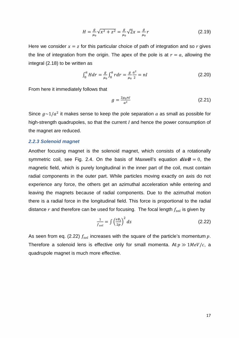
2.2.3 Solenoid magnet

Another focusing magnet is the solenoid magnet, which consists of a rotationally

symmetric coil, see Fig. 2.4. On the basis of Maxwell’s equation 𝒅𝒊𝒗𝑩 = 0, the

magnetic field, which is purely longitudinal in the inner part of the coil, must contain

radial components in the outer part. While particles moving exactly on axis do not

experience any force, the others get an azimuthal acceleration while entering and

leaving the magnets because of radial components. Due to the azimuthal motion

there is a radial force in the longitudinal field. This force is proportional to the radial

distance 𝑟 and therefore can be used for focusing. The focal length 𝑓𝑠𝑜𝑙 is given by

1𝑓𝑠𝑜𝑙

= ∫ �𝑒𝐵𝑠2𝑝�2𝑑𝑠 (2.22)

As seen from eq. (2.22) 𝑓𝑠𝑜𝑙 increases with the square of the particle’s momentum 𝑝.

Therefore a solenoid lens is effective only for small momenta. At 𝑝 ≫ 1𝑀𝑒𝑉/𝑐, a

quadrupole magnet is much more effective.

17

Figure 2.4: Scheme of a solenoid magnet with field lines and particle trajectories.

2.3 Transformation Matrices

To determine the motion of particles, first we write the general equation of motion in

the moving coordinate system 𝐾 = (𝑥, 𝑧, 𝑠) (Fig. 2.1). In general the bending strength

1/𝜌 and the focusing strength 𝑘 are functions of the path length 𝑠 along the reference

orbit. The linear equation of motion for the particles are [2]

𝑥′′(𝑠) + �1

𝜌2(𝑠) − 𝑘(𝑠)�𝑥(𝑠) =1𝜌∆𝑝𝑝

(2.23)

𝑧′′(𝑠) + 𝑘(𝑠)𝑧(𝑠) = 0

where 𝑝 is the nominal momentum of the particles and ∆𝑝 is the momentum

deviation. The general solution 𝑥(𝑠) is the sum of the general solution 𝑥ℎ of the

homogeneous equation and a particular solution 𝑥𝑖 of the inhomogeneous equation

𝑥(𝑠) = 𝑥ℎ(𝑠) + 𝑥𝑖(𝑠) (2.24)

With

𝑥ℎ′′(𝑠) + �1

𝜌2(𝑠) − 𝑘(𝑠)�𝑥ℎ(𝑠) = 0

(2.25)

𝑥𝑖′′(𝑠) + �1

𝜌2(𝑠) − 𝑘(𝑠)�𝑥𝑖(𝑠) =1𝜌∆𝑝𝑝

Since ∆𝑝/𝑝 is assumed to be constant it is obvious that if 𝑥𝑖 is a solution for a given

∆𝑝/𝑝, 𝑛 ∙ 𝑥𝑖 will be a solution for 𝑛 ∙ ∆𝑝/𝑝. Therefore it is useful to normalize 𝑥𝑖 with

respect to ∆𝑝/𝑝:

𝐷(𝑠) = 𝑥𝑖∆𝑝𝑝

(2.26)

18

𝐷(𝑠) is the dispersion trajectory, defined as a particular solution of the following

inhomogeneous equation

𝐷′′(𝑠) + � 1𝜌2(𝑠) − 𝑘(𝑠)�𝐷(𝑠) = 1

𝜌(𝑠) (2.27)

It describes the momentum-dependent part of the motion. The general solution of

(2.23) now reads as

𝑥(𝑠) = 𝐶(𝑠)𝑥0 + 𝑆(𝑠)𝑥0′ + 𝐷(𝑠)∆𝑝𝑝

(2.28)

𝑧(𝑠) = 𝐶(𝑠)𝑧0 + 𝑆(𝑠)𝑧0′

Here 𝑥0 and 𝑧0 are the initial values of the horizontal and vertical displacements, 𝑥0′

and 𝑧0′ the initial values of the horizontal and vertical slopes from the nominal

trajectory. Here 𝐷0 = 𝐷0′ = 0 are considered as initial conditions. 𝐶(𝑠) and 𝑆(𝑠) are

two independent solutions of the homogeneous equation:

𝐶′′(𝑠) + �1

𝜌2(𝑠) − 𝑘(𝑠)�𝐶(𝑠) = 0,

(2.29)

𝑆′′(𝑠) + �1

𝜌2(𝑠) − 𝑘(𝑠)�𝑆(𝑠) = 0.

The solutions which satisfy the initial conditions 𝐶0 = 1,𝐶0′ = 0, 𝑆0 = 0, 𝑆0′ = 1, are

called “Cosinelike” and “Sinelike” trajectories.

The particle coordinates are related to their initial values by a linear transformation,

which can also be described by transfer matrices

�𝑥𝑥′

∆𝑝/𝑝�𝑠

= �𝐶 𝑆 𝐷𝑥𝐶′ 𝑆′ 𝐷𝑥′0 0 1

��𝑥𝑥′

∆𝑝/𝑝�0

,

(2.30)

�𝑧𝑧′

∆𝑝/𝑝�𝑠

= �𝐶 𝑆 0𝐶′ 𝑆′ 00 0 1

��𝑧𝑧′∆𝑝𝑝

�

0

.

The matrix notation of the solution of the equations of motion is particularly useful if

the bending strength 1/𝜌(𝑠) and the focusing strength 𝑘(𝑠) are constant, because in

this case the matrix elements can be expressed analytically. The solution for the

complete magnetic system is then the product of the individual matrices in the

desired sequence. The transfer matrices of the most important magnets are

19

discussed in the following. They may be used as building blocks to assemble the

complete magnetic lattice. To simplify the derivations, it is assumed that the magnetic

fields at the input and output of the components have a step function form (hard edge

approximation).

2.3.1. Drift space

In a drift space, no external force acts on the particles. The transformation matrix

depends only on the length 𝐿 of the drift space.

1𝜌(𝑠) = 0 and 𝑘(𝑠) = 0 → 𝑀𝑥 = 𝑀𝑧 = �

1 𝐿 00 1 00 0 1

� (2.31)

2.3.2. Dipole sector magnet

A dipole magnet whose edges are perpendicular to the ideal orbit is called sector

magnet (Figure 2.5). This magnet acts only on the horizontal direction. In the vertical

direction the particle trajectory is like in the drift space

𝑘(𝑠) = 0 and 𝜑 = 𝑙𝜌 → 𝑀𝑥 = �

𝐶𝑜𝑠𝜑 𝜌𝑆𝑖𝑛𝜑 𝜌(1 − 𝐶𝑜𝑠𝜑)− 1

𝜌𝑆𝑖𝑛𝜑 𝐶𝑜𝑠𝜑 𝑆𝑖𝑛𝜑0 0 1

�, 𝑀𝑧 = �1 𝑙 00 1 00 0 1

�

(2.32)

Figure 2.5 Sector dipole magnet.

2.3.3. Quadrupole magnet

For the quadrupole magnet we have 1𝜌(𝑠)

= 0. If 𝑘 > 0,

𝑀𝑥 =

⎝

⎜⎛

𝐶𝑜𝑠ℎ𝜑1

�|𝑘| 𝑆𝑖𝑛ℎ𝜑 0

�|𝑘| 𝑆𝑖𝑛ℎ𝜑 𝐶𝑜𝑠ℎ𝜑 00 0 1⎠

⎟⎞

(2.33)

20

𝑀𝑧 = �𝐶𝑜𝑠𝜑 1

�|𝑘| 𝑆𝑖𝑛𝜑 0

−�|𝑘| 𝑆𝑖𝑛𝜑 𝐶𝑜𝑠𝜑 00 0 1

�,

where 𝜑 = 𝑙�|𝑘|. These matrices describe horizontal defocusing and vertical

focusing. For the case 𝑘 < 0 the matrices 𝑀𝑥 and 𝑀𝑧 are interchanged and we get

horizontal focusing and vertical defocusing.

In many practical cases, the focal length 𝑓 of the quadrupole magnet is much longer

than the length of the lens:

𝑓 = 1𝑘𝑙≫ 𝑙 (2.34)

In these cases the transfer matrices can be approximated by

𝑀𝑥 = �

1 0 01𝑓

1 0

0 0 1

�

(2.35)

𝑀𝑧 = �−

1 0 01𝑓

1 0

0 0 1

�

Note that these matrices describe a lens of zero length, i.e. they are derived from Eq.

(2.33) using 𝑙 → 0 while keeping 𝑘 ∙ 𝑙 = 𝑐𝑜𝑛𝑠𝑡. The true length 𝑙 of the lens has to be

recovered by two drift spaces 𝑙/2 on either side, e.g.

𝑀𝑥 = �1

𝑙2

00 1 00 0 1

��

1 0 01𝑓

1 0

0 0 1

��1

𝑙2

00 1 00 0 1

� =

⎝

⎜⎜⎛

1 +𝑙

2𝑓𝑙 +

𝑙2

4𝑓0

1𝑓

1 +𝑙

2𝑓0

0 0 1⎠

⎟⎟⎞

(2.36)

𝑀𝑧 = �1

𝑙2

00 1 00 0 1

��

1 0 0

−1𝑓

1 0

0 0 1

��1

𝑙2

00 1 00 0 1

� =

⎝

⎜⎜⎛

1 −𝑙

2𝑓𝑙 −

𝑙2

4𝑓0

−1𝑓

1 −𝑙

2𝑓0

0 0 1⎠

⎟⎟⎞

2.3.4. Solenoid magnet

21

The transfer matrices of solenoid magnets can’t be divided into vertical and

horizontal sub matrices, because of the coupling between particle motions in two

transverse planes. For the short solenoid magnet the transformation matrix for the 4D

vector (𝑥; 𝑥′; 𝑧; 𝑧′) is presented. The short lens approximation is done as in case of

quadrupoles. For that purpose, the transfer matrix 𝑀 of the whole solenoid is

presented as the product of three different matrices 𝑀1,𝑀2,𝑀3 corresponding to the

entrance fringe field, the constant axial magnetic field, and the output fringe field,

respectively.

The radial component of the magnetic field induces an angular kick which changes

the divergence of the beam. Assuming the kick is localized at a given longitudinal

position at the entrance of the solenoid, the matrix 𝑀1 is [3]

𝑀1 =

⎝

⎜⎛

1 0 0 00 1 𝑒𝐵

2𝑃0

0 0 1 0− 𝑒𝐵

2𝑃0 0 1⎠

⎟⎞

(2.37)

with the approximation 𝑃𝑠 ≅ 𝑃. At the output of the solenoid, the matrix has the same

form with an opposite sign in the kick:

𝑀3 =

⎝

⎜⎛

1 0 0 00 1 − 𝑒𝐵

2𝑃0

0 0 1 0𝑒𝐵2𝑃

0 0 1⎠

⎟⎞

. (2.38)

The transfer matrix for the part inside of the solenoid magnet is given by:

𝑀2 =

⎝

⎜⎛

1 𝑃𝑒𝐵𝑆𝑖𝑛𝜃 0 𝑃

𝑒𝐵(1 − 𝐶𝑜𝑠𝜃)

0 𝐶𝑜𝑠𝜃 0 𝑆𝑖𝑛𝜃0 − 𝑃

𝑒𝐵(1 − 𝐶𝑜𝑠𝜃) 1 𝑃

𝑒𝐵𝑆𝑖𝑛𝜃

−𝑆𝑖𝑛𝜃 0 0 𝐶𝑜𝑠𝜃 ⎠

⎟⎞

(2.39)

For the whole solenoid the product of the three matrices, 𝑀 = 𝑀3・𝑀2・𝑀1 gives

the final transformation matrix:

𝑀2 = �

𝐶2 𝐶𝑆/𝛼 𝐶𝑆 𝑆2/𝛼−𝐶𝑆𝛼 𝐶2 −𝑆2𝛼 𝐶𝑆−𝐶𝑆 −𝑆2𝛼 𝐶2 𝐶𝑆/𝛼𝑆2𝛼 −𝐶𝑆 −𝐶𝑆𝛼 𝐶2

� (2.40)

22

with 𝑆 = 𝑆𝑖𝑛(𝜃/2), 𝐶 = 𝐶𝑜𝑠(𝜃/2), 𝛼 = 𝑒𝐵2𝑃

and 𝜃 = 2𝐿𝛼 where 𝐿 is the total length of

the solenoid. The thin lens approximation is done by assuming that the length 𝐿is

small compared to 1/𝛼. By keeping the first terms of Taylor expansions for 𝐶𝑜𝑠𝜃

and 𝑆𝑖𝑛𝜃, the matrix is simplified and takes the form:

𝑀 =

⎝

⎜⎛

1 0 0 0−1

𝑓1 0 0

0 0 1 00 0 −1

𝑓1⎠

⎟⎞

, (2.41)

where 𝑓 is the focal length given by: 1𝑓

= �𝑒𝐵2𝑃�2𝐿.

3. Phase Space ellipse, emittance and Twiss parameters

The matrix formalism presented above allows us to calculate individual particle

trajectories through an arbitrary magnetic system (lattice), taking into account

variations (first order) in particle momentum. However, it does not yield any

information about the properties of the particle ensemble/beam. Since this is

ultimately a decisive factor in the development of the magnetic guide system, we

must extend our techniques to describe the behavior of a particle beam. To do this let

us consider the equation of motion for a particle with nominal energy (∆𝑝/𝑝 = 0) [2]:

𝑦′′(𝑠) + 𝐾(𝑠)𝑦(𝑠) = 0 �𝐾 = 𝑘 𝑓𝑜𝑟 𝑦 = 𝑧

𝐾 = −𝑘 + 1𝜌2

𝑓𝑜𝑟 𝑦 = 𝑥 (3.1)

where 𝐾(𝑠) is a function of position 𝑠.

The trajectory function 𝑦(𝑠) describes a transverse oscillation around the design

orbit, known as a betatron oscillation, whose amplitude and phase depend on the

position 𝑠 along the orbit.

The general solution of the equation (3.1) and its derivative are [2]

𝑦(𝑠) = 𝐴�𝛽(𝑠)𝐶𝑜𝑠(Ψ(𝑠) + 𝜙), (3.2)

𝑦′(𝑠) = − 𝐴�𝛽(𝑠)

[𝛼(𝑠)𝐶𝑜𝑠(Ψ(𝑠) + 𝜙) + 𝑆𝑖𝑛(Ψ(𝑠) + 𝜙)], (3.3)

where 𝛽(𝑠) represents the beta function, 𝛼(𝑠) = 12𝛽′(𝑠) and 𝐴 is the constant of

integration which is defined by the initial conditions and remains constant throughout

23

the whole beam transport system. Thus, within a magnetic structure the particles

perform betatron oscillations with a position-dependent amplitude given by

𝐸(𝑠) = 𝐴�𝛽(𝑠) (3.4)

called the beam envelope. Since all particle trajectories lie inside the envelope 𝐸(𝑠),

it defines the transverse size of the beam (fig. 3.1).

Figure 3.1. Particle trajectories 𝑦(𝑠) within the envelope 𝐸(𝑠) of the beam.

The beta function 𝛽(𝑠) is a measure of the beam cross-section. It is defined by the

magnetic lattice and varies with the position.

In order to arrive at an expression describing the particle motion in the 𝑦 − 𝑦′ phase

space we must eliminate the terms which depend on the phase Ψ. From (3.2) and

(3.3) we immediately obtain

𝐶𝑜𝑠(Ψ(𝑠) + 𝜙) = 𝑦𝐴�𝛽(𝑠)

, (3.5)

𝑆𝑖𝑛(Ψ(𝑠) + 𝜙) = �𝛽(𝑠)𝑦′

𝐴+ 𝛼(𝑠)𝑦

𝐴�𝛽(𝑠) . (3.6)

If we now use the relation 𝑆𝑖𝑛2Θ + 𝐶𝑜𝑠2Θ = 1 we obtain

𝑦2

𝛽(𝑠) + � 𝛼(𝑠)�𝛽(𝑠)

+ �𝛽(𝑠)𝑦′�2

= 𝐴2 . (3.7)

With the definition

𝛾(𝑠) = 1+𝛼2(𝑠)𝛽(𝑠) (3.8)

the eq. (3.7) transformes into

𝛾(𝑠)𝑦2(𝑠) + 2𝛼(𝑠)𝑦(𝑠)𝑦′(𝑠) + 𝛽(𝑠)𝑦′2(𝑠) = 𝐴2 . (3.9)

y[mm]

envelope

24

This is the general equation of an ellips in the 𝑦 − 𝑦′ plane (Fig. 3.2). The area of the

phase space ellipse is an important quantity. It is given by 𝜋𝐴2.

Let us now consider a particle beam filling the phase space up to the ellipse with

amplitude 𝐴𝑚𝑎𝑥. According to Louville’s fundamental theorem [2] the phase space

density of particles in the vicinity of any phase space trajectory is invariant if the

particles obey the canonical equations of motion. This condition is generally satisfied

in accelertors under the condition that the partice energy remains constant and the

stochastic effects like beam-gas scattering or synchrotron radiation are negligible.

This means that the area of the enclosing phase ellipse is an invariant of the beam

motion. As the particles move along the orbit the shape and position of individual

ellipses as well as of the enclosing ellipse change according to the amplitude function

𝛽(𝑠), but areas remain constant. This result has important consequences for the

calculation of linear beam optics. The area of the enclosing ellipse of the beam is

denoted by 𝜋𝜀, where 𝜀 is called the beam emittance.

Figure 3.2. The phase space ellipse in the horizontal plane.

When the particles are accelerated, the emittance decreases inversely proportional

to the momentum. This can be understood intuitively from the observation that only

the longitudinal component of the momentum vector is increased in the accelerating

section whereas the transverse components remain invariant, so that the beam

divergence shrinks. Therefore we also define the normalized emittance 𝜀𝑛 which

remains constant during acceleration.

𝜀𝑛 = 𝛾𝛽𝜀 (3.10)

where 𝛾 is the Lorentz factor, and 𝛽 = 𝑣/𝑐.

25

3.1. Transformation of the beta function

The orientation of the phase ellipse at a point 𝑠 is characterized by the Twiss

parameters 𝛼(𝑠), 𝛽(𝑠), 𝛾(𝑠) and the area is determined by the emitance 𝜀.

It is important to know the beam envelope and divergence at each point of the

accelerator. Therefore, it is of great interest to know how 𝛼,𝛽, 𝛾 are transformed

through the magnetic system.

We evaluate the invariant 𝐴 for a single particle at a reference point 𝑠0 and an

arbitrary other point 𝑠.

𝐴2 = 𝛾𝑦2 + 2𝛼𝑦𝑦′ + 𝛽𝑦′2 = 𝛾0𝑦02 + 2𝛼0𝑦0𝑦0′ + 𝛽0𝑦0′2 (3.11)

Using the principal trajectories we can relate 𝑦(𝑠),𝑦′(𝑠) to 𝑦0 = 𝑦(𝑠0),𝑦0′ = 𝑦′(𝑠0)

�𝑦𝑦′� = �𝐶 𝑆

𝐶′ 𝑆′� �𝑦0𝑦0′� (3.12)

The inverse transformation matrix is � 𝑆′ −𝑆

−𝐶′ 𝐶 � so

𝑦0 = 𝑆′𝑦 − 𝑆𝑦′ (3.13)

𝑦0′ = −𝐶′𝑦 + 𝐶𝑦′ (3.14)

𝐴2 = 𝛾0(𝑆′𝑦 − 𝑆𝑦′)2 + 2𝛼0(𝑆′𝑦 − 𝑆𝑦′)(−𝐶′𝑦 + 𝐶𝑦′) + 𝛽0(−𝐶′𝑦 + 𝐶𝑦′)2 =

= 𝛾𝑦2 + 2𝛼𝑦𝑦′ + 𝛽𝑦′2 (3.15)

Comparing the coefficients yields:

𝛽(𝑠) = 𝐶2𝛽0 − 2𝑆𝐶𝛼0 + 𝑆2𝛾0 (3.16)

𝛼(𝑠) = −𝐶𝐶′𝛽0 + (𝑆𝐶′ + 𝑆′𝐶)𝛼0 − 𝑆𝑆′𝛾0 (3.17)

𝛾(𝑠) = 𝐶′2𝛽0 − 2𝑆′𝐶′𝛼0 + 𝑆′2𝛾0 (3.18)

In matrix notation

�𝛽𝛼𝛾� = �

𝐶2 −2𝑆𝐶 𝑆2−𝐶𝐶′ 𝑆𝐶′ + 𝑆′𝐶 −𝑆𝑆′

𝐶′2 −2𝑆′𝐶′ 𝑆′2� �

𝛽0𝛼0𝛾0� (3.19)

By means of this matrix equation one can transform the beta function piece-wisely

through the magnets and drift spaces.

26

3.2. The Beam matrix

The transverse emittance for a well-centered and aligned beam (⟨𝑥⟩, ⟨𝑧⟩, ⟨𝑥′⟩, ⟨𝑧′⟩ = 0)

can be determined as [4]

𝜀𝑥 = �𝑑𝑒𝑡𝜎𝑥 , 𝜀𝑧 = �𝑑𝑒𝑡𝜎𝑧 , (3.20)

where

𝛔𝑥 = �σ11x σ12xσ21x σ22x

� = �< 𝑥2 > < 𝑥𝑥′ >< 𝑥𝑥′ > < 𝑥′2 >

� (3.21)

𝛔𝑧 = �σ11z σ12zσ21z σ22z

� = �< 𝑧2 > < 𝑧𝑧′ >< 𝑧𝑧′ > < 𝑧′2 >

�

Fig. 3.3 shows the beam ellipse in the 𝑥 − 𝑥′ plane, where its tilt angle and

dimensions are expressed by means of the elements of the beam matrix.

Figure 3.3. Beam ellipse.

The matrix element 𝜎11 is the square of the standard deviation of the transverse

beam distribution

Σ𝑥,𝑧 = �σ11𝑥,𝑧

The equation of the phase space ellipse can be written in a different way by using

symmetric two dimensional beam matrices

(𝑥, 𝑥′)σ𝑥−1 �𝑥𝑥′� = 1 (3.23)

(𝑧, 𝑧′)σ𝑦−1 �𝑧𝑧′� = 1 (3.24)

Since σ12 = σ21 this can be written by

27

σ22𝑥2 − 2σ21𝑥𝑥′ + σ11𝑥′2 = 𝑑𝑒𝑡𝛔𝑥 = 𝜀x2

(with Eq. (3.20)) (3.25)

Comparison with Eq. (3.11) yields the following relations between the Twiss

parameters, the emittance, and the beam matrix:

𝛔𝑥 = �σ11𝑥 σ12𝑥σ21𝑥 σ22𝑥

� = 𝜀𝑥 �𝛽𝑥 −𝛼𝑥−𝛼𝑥 𝛾𝑥

�

𝛔𝑧 = �σ11𝑧 σ12𝑧σ21𝑧 σ22𝑧

� = 𝜀𝑥,𝑧 �𝛽𝑧 −𝛼𝑧−𝛼𝑧 𝛾𝑧

� (3.26)

The transformation of the beam matrix from the position 𝑠0 to 𝑠 can be calculated by

σ𝑠 = 𝑀σ𝑠0𝑀𝑇, (3.27)

where 𝑀 is the transfer matrix from position 𝑠0 to 𝑠.

3.3 FODO structure

In accelerators it is necessary to transport charged particle beams over a long

distance without the beam cross-section becoming too large. The simplest

arrangement of magnets for this task is the FODO structure (Fig 3.4). It is composed

of focusing (F) and defocusing (D) quadrupoles separated by a focusing-free section

(O). Since quadrupoles focus only in one plane while defocusing in the other plane,

the magnets are arranged one after another with alternating polarity. As a result the

FODO system has an overall focusing effect on a beam.

Figure 3.4. FODO structure.

Let us derive the transfer matrices of a FODO structure under the thin lens

approximation and assumption that focal lengths are the same for both

quadrupoles 𝑓𝐹 = −𝑓𝐷 = 𝑓 and the magnets are separated by a drift space. The

horizontal transfer matrix of the FODO cell can be calculated by

𝑀𝐹𝑂𝐷𝑂,𝑥 = 𝑀𝑓𝑀𝑑𝑟𝑖𝑓𝑡𝑀𝑑𝑀𝑑𝑟𝑖𝑓𝑡𝑀𝑓 (3.28)

28

Where 𝑀𝑓 and 𝑀𝑑 are the transfer matrices of the focusing and defocusing

quadrupoles respectively and 𝑀𝑑𝑟𝑖𝑓𝑡 is the transfer matrix for drift space.

𝑀𝐹𝑂𝐷𝑂,𝑥 =

⎝

⎜⎛

1 − 𝑙2

2𝑓22𝑙(1 + 𝑙

2𝑓) 0

− 𝑙𝑓2�1 − 𝐿

2𝑓� 1 − 𝑙2

𝑓20

0 0 1⎠

⎟⎞

(3.29)

The transfer matrix of a FODO cell for the vertical plane can be obtained by replacing

𝑓 by – 𝑓.

𝑀𝐹𝑂𝐷𝑂,𝑧 =

⎝

⎜⎛

1 − 𝑙2

2𝑓22𝑙(1 − 𝑙

2𝑓) 0

− 𝑙𝑓2�1 + 𝐿

2𝑓� 1 − 𝑙2

𝑓20

0 0 1⎠

⎟⎞

(3.30)

The matrix element 𝑀21 giving the total focusing/defocusing strength of the system is

negative in both cases as long as L<2f, thus providing focusing effect of FODO cell in

both planes.

4. Electron Beam Parameter Measurements at AREAL Linac

The lab work consists of two parts. In the (preparatory) PART 1 of the lab work, the

students are given an overview of AREAL linac diagnostics, the control system and

some background on operation principles. They learn how to work with machine main

control tools and to manipulate with electron beam parameters. In the (experimental)

PART 2 of the work, the students will perform measurements of the electron beam

transverse emittances and beam energy/energy spread. Upon completion of the lab

work, students are expected to obtain basic knowledge of electron beam diagnostic

methods and hands-on experience in measurement of electron beam main

parameters.

4.1. Introduction

Beam diagnostics and instrumentation are an essential part of any accelerator. There

is a large variety of parameters to be measured for observation of particle beams

with the precision required to tune, operate, and improve the performance of the

machine [5].

29

One of the 1-st questions in the commissioning of a new accelerator is how many

particles are in the machine. Thus the beam intensity (bunch current/charge) is one

of the most important accelerator parameters. With knowledge of the intensity it is

possible to determine lifetime and coasting beam in circular machines, or transfer

efficiencies in linacs and transfer lines.

One of the next questions which arise may be where these particles are located, i.e.,

the position of the beam centroid. Position measurements give access to a wide

number of very important accelerator parameters. The most fundamental one is the

determination of the beam orbit.

The next question might be how the distribution of particles in space looks, i.e.,

beam profiles in both transversal and longitudinal dimensions are of interest. Beam

size measurements are fundamental for the determination of the beam emittance.

Emittance is an important property of charged particle beams, allowing for a

description of beam quality and the comparison of beams, as emittance is a constant

of motion in many cases.

Another parameter of interest is the beam energy. In synchrotron light sources (third-

generation storage rings, as well as free-electron-lasers (FELs)) it defines the

spectral characteristics of the emitted radiation. In electron accelerators, the energy

distribution of the electron beam is another essential parameter for the study of the

longitudinal beam dynamics and beam instabilities.

Currently in the AREAL linac, measurements of electron beam charge, transverse

beam shape/size, transverse beam emittances and beam energy/energy spread [6]

are foreseen. The schematic layout of the AREAL facility’s current state is presented

in Fig. 4.1.

Figure 4.1. Layout of the AREAL electron gun section with diagnostics. Abbreviations are explained in the text.

30

The current lab work covers measurements of beam energy/energy spread and

transverse beam emittances. Both experiments are based on on beam transverse

profile measurement.

Beam profile diagnostics are used both for initial tuning of the beam position and

beam spot size. A beam spot is the main source of information used to monitor and

study the beam transport as well as transverse beam distribution.

The determination of the transverse beam profiles relies on the interaction of beam

particles with matter. The method mostly applied is destructive to the beam as it hits

a luminescent screen. A part of the deposited energy results in excited electronic

states which de-excite partially via light emission. Therefore, the beam profile can be

observed via a CCD camera. Sometimes screens are even used as beam position

monitors by analyzing the center of gravity of the measured light distribution.

In the AREAL linear accelerator, for beam profile measurements only scintillator

crystal (YAG:Ce) based stations are installed. This type of measurement technique is

used since for the AREAL electron beam parameters the other possible systems

(such as screens based optical transition radiation (OTR) or the wire scanner) would

not generate sufficient signal-to-noise ratio.

Two stations are placed in the low energy diagnostic line of the AREAL linear

accelerator (Fig. 4.1). Both stations are based on YAG:Ce crystals with 25x25x0.2

mm dimensions. The crystals are mounted to a holder and positioned in the beamline

by pneumatic linear motion motors. The scintillators are mounted at the right angle to

the beam motion and the emitted light beam repeats the electron beam transverse

size in the same direction. The station has two reflecting mirrors. The first mirror is

mounted by 450 with light direction and reflects the light out of the vacuum chamber.

The second mirror is also mounted by 450 towards the reflected light from the first

mirror and reflects the light by the optical tube to a camera (Fig. 4.2). Since both

mirrors are located under 450 to the direction of the photon beams, the beam size is

not changed during transportation through the projection on mirrors.

31

Figure 4.2. Schematic layout of the beam profile measurement

A Point Gray Flea2 08S2 CCD camera at position YAG1 (1032x776 pixels with 4.65

μm size) and a Flea2 20S4 CCD camera (1624x1224 pixels with 4.4 μm size) at YAG

2 stations are used for electron beam transverse profile registration (see Fig. 4.1).

The CCD camera signal is transported from the tunnel to the control system via a

repeater/HUB. The image is digitized, the beam spot is projected onto orthogonal

axes and the statistical properties of the distribution are calculated. The calibration of

scales is obtained using reference marks on the screen.

The measurement accuracy of the screen station mainly depends on 3 factors:

• photon beam size deviation from the original electron beam size

• optical system resolution

• data registration and analysis

Photon beam size deviation from the original beam size occurs due to the multiple

scattering of the electrons. Passing through a matter, primary electrons are scattered

and create secondary electrons and photons, this changes the original direction of

their movement. Because of this, the image of the point source will be seen as a

distribution with a finite RMS size. As a result, the electron beam image on the CCD

camera will be bigger than the real sizes of the beam. YAG crystals at AREAL have

0.2 mm thickness and for 5 MeV beam energy the estimations give 30 μm RMS size

of the point electron source.

32

Another reason of the measurement accuracy degradation is the optical system

resolution. At both stations objectives with the same 75 mm focusing lengths of 100

pair/mm resolution are used (5 μm on the photon beam). Later the photon beam is

registered by CCD sensors. At YAG1 and YAG2 stations we have 1:7.5 and 1:5

image magnifications, respectively. At YAG1 station 1 pixel corresponds to 34.875

μm beam size and the CCD sensor covers 36x27 mm2 area of the YAG holder. At

YAG2 station the CCD sensor covers 36x26 mm2 area of the YAG holder and has a

22 μm to 1-pixel transformation.

4.2. Beam energy and energy spread measurements

The measurements of electron beam momentum (energy) and momentum spread

(energy spread) are usually done with a magnet spectrometer [5]. The spectrometer

transforms the momentum (spread) into a position (spread), as shown in Fig. 4.3,

which is measured with a spatial resolving detector (for example YAG screen)

according to ∆𝑥𝑥0

= ∆𝑝𝑝0

. (4.1)

Figure 4.3. Principle of a magnet spectrometer for the momentum (energy) and momentum spread (energy spread) determination.

At the AREAL gun section, a 90° bending magnet is used as a spectrometer. The

dipole magnet bends the electron beam, and the beam position is registered by the

YAG 2 station. Then the beam momentum p (energy) is calculated based on the

geometry and calibration of the dipole magnet and the alignment of YAG 2 screen:

𝑝 = 𝑞𝑙𝐵𝛼

, (4.2)

where q is the electron charge, B the magnetic field of the dipole magnet, 𝑙 is the

effective magnetic length and α is the bending angle of the dipole.

33

The magnetic field of the AREAL spectrometer dipole magnet can be changed from 0

to 200 mT by 0.25 mT steps and has 𝑙 = 15.34 𝑐𝑚 effective length. Thus the beam

momentum (energy) can be determined by

𝑝 �𝑀𝑒𝑉𝑐� = 0.02888 𝐵[𝑚𝑇]. (4.3)

Please verify this relation! The beam energy measurement accuracy depends on

magnetic field determination and beam center registration accuracy. Since the

determination accuracy of the dipole magnet field is better than 0.25mT, the beam

energy measurement accuracy it is about 7.7 keV, which is less than 0.15% for 5

MeV beam energy. The beam registration accuracy at YAG 2 screen is about 50 μm

which causes a maximum 0.0625 MeV energy measurement error. This is about 1.25

% for 5 MeV beam energy.

The energy spread is estimated by observing the beam in a dispersive section where

the beam horizontal spot size is a convolution of the emittance and dispersion

contributions [2]. It can be written to first order as:

𝜎𝑥 ≈ �𝛽𝑥𝜀𝑥 + 𝐷𝑥2𝜎𝐸2 , (4.4)

where 𝜎𝑥 is the horizontal beam size at the YAG 2 screen located behind the bending

at spectrometer arm, 𝜀𝑥 is the horizontal emittance, 𝛽𝑥 and 𝐷𝑥 are the horizontal beta

and dispersion functions and 𝜎𝐸 is the rms energy spread of the beam, respectively.

Thus, for the measured energy spread we find:

𝜎𝐸 =�𝜎𝑥2−𝛽𝑥𝜀𝑥

|𝐷𝑥|≤ 𝜎𝑥

|𝐷𝑥| . (4.5)

In order to maximize the momentum resolution of the spectrometer, the dispersive

contribution to the beam size should be large compared with the emittance

contribution (𝛽𝑥𝜀𝑥 ≪ 𝐷𝑥2𝜎𝐸2). This is achieved by providing horizontal focus (with the

help of a solenoid magnet) at YAG 2, thus minimizing 𝛽𝑥.

4.2.1. Electron beam energy and energy spread measurement control tools

For beam energy/energy spread measurements “Dipole_Control” and “Beam_Profile”

tools are used. The “Dipole_Control” tool (Fig. 4.4) suggests two options for magnetic

field modification: with and without cycling. In the first case the magnetic field is

changed taking into account the hysteresis effect.

34

Figure 4.4. “Dipole_Control” tool layout.

The tool consists of the following sections:

Table 4.1. Sections of the Dipole_Control tool.

Section 1: DAQ Disconnect - Magnet On

Connect - Magnet Off

Section 2: Current Current - magnet power supply current in A

Set - set input value for current

Section 3: Magnet parameters Voltage - power supply voltage in V

Magnetic Field - Magnetic field in mT

The interface and sections of the “Beam_Profile” tool are given in Fig. 4.5 and Table

4.2.

3

1

2

35

Figure 4.5. Beam_Profile tool layout.

Table 4.2. Sections of the Beam_Profile tool.

Section 1: Camera

Select Camera - select camera for beam registration

Units (𝒑𝒙,𝒑𝒚) - camera pixel to mm interpretation

coefficients

Set - click to set coefficients

Section 2: Camera Option

Gain - camera gain value

Brightness - camera brightness value

Shutter - camera shutter value

Section 3: Preview On - switch on camera on preview mode

Off - switch off camera

Section 4: Background

Start - start background data scan

Stop - stop background data scan

Calculated over - background data calculation period

Exclude background - select to exclude background in

Section 5 view and calculation of results in Section 6

Section 5: Beam profile

Start - start beam registration and data analysis

Stop - stop beam registration and data analysis

Beam Profile - registered beam transverse profile

Fit - horizontal/vertical fit of the beam intensity

Section 6: Results X position - horizontal position of the beam center

5

6

7

8

1 2 3 4

36

Y position - vertical position of the beam center

X rms - horizontal rms size of the beam profile

Y rms - vertical rms size of the beam profile

Section 7: Camera parameters

Camera - selected camera name

px/py - camera pixel to mm interpretation coefficients

Mode - show camera run mode

Status - camera status (start/stop)

Section 8: Export data Export data - click to save data

For the beam energy spread measurement, a quadrupole magnet is used to

additionally focus the electron beam on YAG 2 screen. The layout of the quadrupole

magnet control tool “Quadrupole_PS” and its sections are given below:

Figure 4.6. Quadrupole_PS tool layout

Table 4.3: Sections of the Quadrupole_PS tool.

Section 1: DAQ Disconnect - Magnet On

Connect - Magnet Off

Section 2: Current Current - magnet power supply current in A

Set - set input value for current

Section 3: Magnet parameters Voltage - power supply voltage in V

Magnetic Field - Magnetic field in mT

4.2.2. Measurement tasks

• Measure the beam energy

2

3

1

37

o Change the magnetic field of the dipole until the beam is observed at

YAG 2 screen.

o Fine tune the position (dipole field) of the beam center such that it

coincides with the YAG 2 crystal center.

o Calculate the beam energy with formula (4.3).

• Estimate the beam energy spread

o After completing the first two steps of the previous task, achieve

maximum horizontal focusing on YAG 2 screen by adjusting the field of

the quadrupole magnet.

o Measure the beam spot size by using the “Beam_Profile” control tool.

o Estimate the beam energy spread using formula (4.5) (𝐷𝑥 = 0.2401 𝑚).

4.2.3 Measurement procedure

At the AREAL linac the electron beam energy is measured by the following

procedure:

1. Run “Dipole_Control” tool and press Connect button at the Section 1 (Fig. 4.4).

2. Start “Beam Profile” tool and select camera Gun_YAG2 at the “Select

Camera” field in Section 1 (Fig. 4.5).

3. Push “On” button in Section 3 to register electron beam (Fig. 4.5).

4. Tune the magnet field until the beam is observed by changing the current

value in “Current” field of Section 2 (Fig. 4.4).

5. After the beam observation, switch off the preview mode in Section 3, start the

background scan by pushing the “Start” button in Section 4, then check

“Exclude Background” (Fig. 4.5).

6. Start the beam observation and data analysis by pressing the “Start” button in

Section 5 (Fig. 4.5).

7. Tune the value of the magnet current to move the electron beam to the center

of the screen.

8. Fix the current value and determine the beam energy from the calibration

curve given in Fig. 4.7.

38

Figure 4.7. Dipole magnet current vs electron beam energy at AREAL. The students should discuss, why this curve is not perfectly linear !

In order to estimate the beam energy spread the following steps should be

performed:

1. Start the “Quadrupole_PS” tool after the beam energy measurement

procedure (8 steps described above).

2. Switch on the quadrupole magnet by pushing the “Connect” button in Section

1 (Fig.4.6).

3. Change the current value at the “Current” field of Section 2 to change the

quadrupole strength (Fig. 4.6) until the maximum horizontal focusing at the

YAG2 station is reached (Fig. 4.5).

4. Estimate the beam energy spread using formula (4.5).

4.3. Beam Transverse Emittance Measurements

Emittance is an important property of charged particle beams, allowing for a

description of beam quality and the comparison of beams. One of the most

challenging directions in electron beam physics and accelerator technologies is the

generation of high brightness powerful shortwave electromagnetic radiation. To

generate high brightness powerful radiation, it is mandatory to produce charged

particle beams with low emittance and high energy. The brightness is defined as

𝐵 = 𝐹4𝜋2𝜀𝑥𝜀𝑧

, (4.6)

where F is the photon flux, defined as the number of radiated photons per second

and within spectral bandwidth of 0.1%, 𝜀𝑥 and 𝜀𝑧 are the horizontal and vertical

emittances, respectively.

39

There are different techniques for measuring the transverse beam emittance [7]. In

this course the Solenoid/Quadrupole scan technique will be considered.

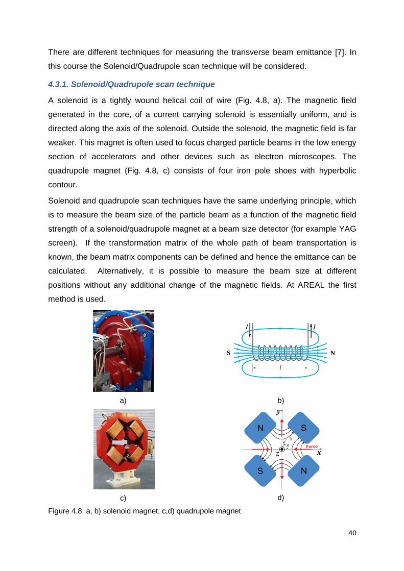
4.3.1. Solenoid/Quadrupole scan technique

A solenoid is a tightly wound helical coil of wire (Fig. 4.8, a). The magnetic field

generated in the core, of a current carrying solenoid is essentially uniform, and is

directed along the axis of the solenoid. Outside the solenoid, the magnetic field is far

weaker. This magnet is often used to focus charged particle beams in the low energy

section of accelerators and other devices such as electron microscopes. The

quadrupole magnet (Fig. 4.8, c) consists of four iron pole shoes with hyperbolic

contour.

Solenoid and quadrupole scan techniques have the same underlying principle, which

is to measure the beam size of the particle beam as a function of the magnetic field

strength of a solenoid/quadrupole magnet at a beam size detector (for example YAG

screen). If the transformation matrix of the whole path of beam transportation is

known, the beam matrix components can be defined and hence the emittance can be

calculated. Alternatively, it is possible to measure the beam size at different

positions without any additional change of the magnetic fields. At AREAL the first

method is used.

a)

b)

c)

d)

Figure 4.8. a, b) solenoid magnet; c,d) quadrupole magnet

40

Let R be the total transformation matrix for the solenoid/quadrupole and drift spaces

from distance 𝑠 to 𝑠0:

𝑅 = �𝑅11 𝑅12𝑅12 𝑅22

�. (4.7)

Recall (see Eq. (3.27)) that the beam matrix at position 𝑠 is related to beam matrix at

𝑠0 by

𝜎(𝑠) = 𝑅(𝑠)𝜎(𝑠0)𝑅𝑇(𝑠). (4.8)

The first term in the resultant matrix is

𝜎11(𝑠) = 𝜎11(𝑠0)𝑅112 + 2𝜎12(𝑠0)𝑅11𝑅12 + 𝜎22(𝑠0)𝑅12

2 . (4.9)

If Q represents the transfer matrix of the solenoid/quadrupole and S represents the

transfer matrix between the solenoid/quadrupole and the imaging screen (Fig. 4.9),

then in the thin lens approximation the transfer matrices may be written as:

𝑅 = �𝑆11 + 𝐾𝑆12 𝑆12𝑆21 + 𝐾𝑆22 𝑆22

�, (4.10)

where (see Eq. (2.35))

𝑄 = �1 0𝐾 1�, 𝑆 = �𝑆11 𝑆12

𝑆21 𝑆22� (4.11)

(K is the integrated field strength 1/f of the solenoid/quadrupole magnet).

Figure 4.9. The schematic layout of the setup.

Thus, eq. (4.9) takes the form

𝜎11(𝑠) = (𝑆11 + 𝐾𝑆12)2𝜎11(𝑠0) + 2𝑆12(𝑆11 + 𝐾𝑆12)𝜎12(𝑠0) + 𝑆122 𝜎22(𝑠0), (4.12)

or

𝜎11(𝑠) = 𝐴𝐾2 + 𝐵𝐾 + 𝐶 (4.13)

where

41

𝐴 = 𝑆122 𝜎11(𝑠0),

𝐵 = 2𝑆11𝑆12𝜎11(𝑠0) + 2𝑆122 𝜎12(𝑠0), (4.14)

𝐶 = 𝑆112 𝜎11(𝑠0) + 2𝑆11𝑆12𝜎12(𝑠0) + 𝑆122 𝜎22(𝑠0).

Acquiring a set of beam size measurements at detector location 𝑠 as the solenoid/

quadrupole field strength is scanned over a range of values (around the value

providing maximal focused beam), and using least squares for parabolic fitting, A, B,

C parameters can be determined. Then beam matrix elements at location 𝑠0 can be

found from (4.14), allowing to calculate the emittance with (3.20).

4.3.2. Emittance determination errors1

Let �⃗� = {𝑥1, 𝑥2, … 𝑥𝑛}𝑇 be n random variables with known covariance matrix V(x). Let

�⃗� = {𝑦1,𝑦2, …𝑦𝑛}𝑇 with 𝑦𝑗 = 𝑦𝑗(𝑥1, 𝑥2, … 𝑥𝑛), are variables dependent on �⃗�. Then the

covariance matrix V(y) is given by [8]

V(y) = B · V (x) · BT (4.15)

where the matrix B is the Jacobian defined as:

𝐵 =

⎝

⎜⎛

მ𝑦1მ𝑥1

მ𝑦1მ𝑥2

… მ𝑦1მ𝑥𝑛მ𝑦2მ𝑥12

მ𝑦2მ𝑥2

…მ𝑦2მ𝑥𝑛

……

მ𝑦𝑚მ𝑥1

მ𝑦𝑚მ𝑥2

…მ𝑦𝑚მ𝑥𝑛

⎠

⎟⎞

(4.16)

In the special case of a linear transformation �⃗� = 𝐵1 · �⃗� , the Jacobian B is simply the

matrix 𝐵1, which defines the linear transformation.

Now, considering (4.9), the entire measurement can be written in a vector form as

follows

⎝

⎜⎛𝜎11

(1)(𝑠)

𝜎11(2)(𝑠)

……𝜎11

(𝑛)(𝑠)

⎠

⎟⎞

�������

=

𝑏�⃗⎝

⎜⎛

𝑅11(1)2 2𝑅11

(1) 𝑅12(1) 𝑅12

(1)2

𝑅11(2)2 2𝑅11

(2) 𝑅12(2) 𝑅12

(2)2……

𝑅11(𝑛)2 2𝑅11

(𝑛) 𝑅12(𝑛) 𝑅12

(𝑛)2

⎠

⎟⎞

�����������������𝑀

· �𝜎11(𝑠0)𝜎12(𝑠0)𝜎22(𝑠0)

������

𝑎�⃗

(4.17)

1 This section is merely a practical reference how to estimate errors of emittance and can not replace the standard statistics lectures.

42

where the index n in brackets indicates the number of performed measurements. The

solution of (possibly over determined) system of equations (4.14) is given by the so-

called normal equation

�⃗� = (𝑀𝑇 · 𝑀)−1 · 𝑀𝑇����������� · 𝑏�⃗𝐵

(4.18)

In the following only the error δΣ of the r.m.s. beam size measurement is going to be

considered. It is important to note that the elements of the vector 𝑏�⃗ in eq. 4.18 are the

squared beam sizes (Σ2 = 𝜎11). If one for example assumes a constant fractional error

of δΣ/Σ = η (e.g. η = 5 %), then the error of the squared beam size δΣ2 ≈ 2ΣδΣ =

2ηΣ2 . Since the individual measurements are independent from each other, the

covariance matrix of the squared beam sizes has a diagonal form

𝑉(𝑏) = 𝑑𝑖𝑎𝑔[𝑣𝑎𝑟(Σ12), 𝑣𝑎𝑟(Σ22), … , 𝑣𝑎𝑟(Σ𝑛2)]=

= 𝑑𝑖𝑎𝑔[4𝜂2Σ14, 4𝜂2Σ24, … , 4𝜂2Σ𝑛4] (4.19)

The procedure of the error estimation consists of two steps or two error propagations

respectively. In the first step the covariance matrix V(a) of the statistical quantities 𝑎𝑖

is obtained straightforward from eq. (4.15) with the matrix B as defined in eq. (4.18)

𝑉(𝑎) = [(𝑀𝑇 · 𝑀)−1 · 𝑀𝑇] · 𝑉(𝑏) · [(𝑀𝑇 · 𝑀)−1 · 𝑀𝑇]𝑇. (4.20)

Remember that the matrix M is known from the calibration of the quadrupole and the

known geometry of the measurement set-up (see eq. (4.7), (4.10), (4.17)).

In the next step, again using eq. (4.15), one obtains the variance

𝑣𝑎𝑟(𝜀𝑥) = 𝐽 · 𝑉(𝑎) · 𝐽𝑇, (4.21)

where 𝐽 = �მƐ𝑥მ𝑎1

, მƐ𝑥მ𝑎2

, მƐ𝑥მ𝑎3� (see eq. (3.20) and (4.17)).

4.3.3. Emittance measurement tool

For the electron beam emittance measurement at AREAL linac, the EMIT tool is

used. The tool consists of eight main sections which are presented in Fig. 4.10. The

tool sections are described in Table 4.4.

43

Table 4.4. Description of EMIT tool. Section 1: Camera selection Cam1-Camera of the YAG1 station

Cam2- Camera of the YAG2 station

Section 2: Magnet selection QF- Quadrupole magnet

Sol - Solenoid magnet

Section 3: Beam image and sizes Beam transverse spot image (intensity map) with projections

into horizontal and vertical axes

Section 4: Beam parameters 𝝈𝒙 – horizontal size

𝝈𝒚 – vertical size

x position – horizontal offset of the registered beam center

y position – vertical offset of the registered beam center

Section 5: Scan parameters Emittance orientation – choose measured emittance

(𝜀𝑥/𝜀𝑦)

Initial value – magnet initial field value for measurement

Step size- magnet field changing size

Step count – number of measurements

Data per measurement- number of measurements in one

step

Section 6: Start/Cancel buttons Start - start emittance measurement Cancel – stop emittance measurement

Section 7: Fit window Equation – quadratic equation of the fit curve

Save result – save measurement data and calculation

results

Section 8: Results 𝝈𝟏𝟏,𝝈𝟐𝟐,𝝈𝟑𝟑 – elements of the beam matrix

𝜺𝒙/𝜺𝒚 – value of the measured emittance

44

Figure 4.10. EMIT tool interface.

4.3.4. Measurement tasks

Measure transverse beam emittance using solenoid/quadrupole scan method.

• Deliver electron beam to YAG 1 screen.

• Obtain a minimum spot size (maximum focused beam) changing the

quadrupole field.

• Acquire a set of beam size measurements around the maximum focusing

point.

• Calculate A, B, C parameters using least squares method for parabolic fitting.

• Calculate the beam emittance using formulae (3.20) and (4.14).

4.3.5. Measurement procedure

The measurement procedure of the transverse beam emittance at the AREAL linac

(using quadrupole scan method) is the following:

1. Run the EMIT tool

2. Select Cam1 in Section 1 for beam registration at the YAG1 station

3. Observe the electron beam delivered to the YAG 1 screen in Section 3

4. Select the QF quadrupole magnet in Section 2.

5. Use 0 as initial value for the quadrupole magnetic field, 0.02 step size and 20

steps in Section 5.

1 3 2 4

5 6 7 8

45

6. Push Start button in Section 6 to start measurements.

7. Find the magnet field value for minimum spot size (maximum focused beam)

from the green curve in Section 7.

• Return to Step 5 if the minimum spot size is not reached and use more steps

(for example 40).

8. Use a better initial value of the magnetic field (the initial value must be chosen

so that the beam size measurements are made around the maximum focusing

point), smaller step size (< 0.015), more than 10 steps for better fit of

measurement data and push Start button in Section 6.

• In order, to minimize influence of the beam fluctuations during the measurements,

more than one beam can be registered for one field value (Data per measurement, Section 5). Afterwards, the average of these measurements will

be considered as a beam size in this point.

9. Push Save results button in Section 7 to save the calculated emittance value

and measurement data in a local file.

10. Estimate emittance calculation error by assuming 5% constant fractional error

of δΣ/Σ.

Bibliography

1. K. Wille, Physics of Particle Accelerators, Oxford University Press, 2001.

2. P. Schmüser, J. Rossbach, Basic Course on Accelerator Optics, In CAS-

CERN Accelerator School: 5th General Accelerator Physics Course, 1993.

3. Ph. Royer, Solenoidal Optics, PS/HP Note 99-12, Neutrino Factory Note 11,

1999.

4. H. Wiedemann, Particle Accelerator Physics, Springer, 3ed., 2007.

5. G. Kube, CERN–2009–005, pp. 1-64.

6. A. A. Sargsyan et al., Journal of Instrumentation, T03004, 2017.

7. K. T. McDonald, D. P. Russell, Frontiers of Particle Beams; Observation,

Diagnosis and Correction. Lecture Notes in Physics, v. 343. Springer, 1989.

8. E. Blobel, E. Lohrmann, Statistische und numerische Methoden der

Datenanalyse. Wiesbaden: Teubner, 1998, ISBN 978-3-935702-66-9, (see

Sec 4.9) http://www-ibrary.desy.de/elbook.html

46