Electricity Generation and Emissions Reduction Decisions

under Policy Uncertainty: A General Equilibrium Analysis

Jennifer Morris, Mort Webster and John Reilly

Report No. 260April 2014

The MIT Joint Program on the Science and Policy of Global Change is an organization for research, independent policy analysis, and public education in global environmental change. It seeks to provide leadership in understanding scientific, economic, and ecological aspects of this difficult issue, and combining them into policy assessments that serve the needs of ongoing national and international discussions. To this end, the Program brings together an interdisciplinary group from two established research centers at MIT: the Center for Global Change Science (CGCS) and the Center for Energy and Environmental Policy Research (CEEPR). These two centers bridge many key areas of the needed intellectual work, and additional essential areas are covered by other MIT departments, by collaboration with the Ecosystems Center of the Marine Biology Laboratory (MBL) at Woods Hole, and by short- and long-term visitors to the Program. The Program involves sponsorship and active participation by industry, government, and non-profit organizations.

To inform processes of policy development and implementation, climate change research needs to focus on improving the prediction of those variables that are most relevant to economic, social, and environmental effects. In turn, the greenhouse gas and atmospheric aerosol assumptions underlying climate analysis need to be related to the economic, technological, and political forces that drive emissions, and to the results of international agreements and mitigation. Further, assessments of possible societal and ecosystem impacts, and analysis of mitigation strategies, need to be based on realistic evaluation of the uncertainties of climate science.

This report is one of a series intended to communicate research results and improve public understanding of climate issues, thereby contributing to informed debate about the climate issue, the uncertainties, and the economic and social implications of policy alternatives. Titles in the Report Series to date are listed on the inside back cover.

Ronald G. Prinn and John M. ReillyProgram Co-Directors

For more information, please contact the Joint Program Office Postal Address: Joint Program on the Science and Policy of Global Change 77 Massachusetts Avenue MIT E19-411 Cambridge MA 02139-4307 (USA) Location: 400 Main Street, Cambridge Building E19, Room 411 Massachusetts Institute of Technology Access: Phone: +1.617. 253.7492 Fax: +1.617.253.9845 E-mail: globalchange@mit.edu Web site: http://globalchange.mit.edu/

1

Electricity Generation and Emissions Reduction Decisions under Policy Uncertainty: A General Equilibrium Analysis

Jennifer Morris*†, Mort Webster* and John Reilly*

Abstract

The electric power sector, which accounts for approximately 40% of U.S. carbon dioxide emissions, will be a critical component of any policy the U.S. government pursues to confront climate change. In the context of uncertainty in future policy limiting emissions, society faces the following question: What should the electricity mix we build in the next decade look like? We can continue to focus on conventional generation or invest in low-carbon technologies. There is no obvious answer without explicitly considering the risks created by uncertainty.

This research investigates socially optimal near-term electricity investment decisions under uncertainty in future policy. It employs a novel framework that models decision-making under uncertainty with learning in an economy-wide setting that can measure social welfare impacts. Specifically, a computable general equilibrium (CGE) model of the U.S. is formulated as a two-stage stochastic dynamic program focused on decisions in the electric power sector.

In modeling decision-making under uncertainty, an optimal electricity investment hedging strategy is identified. Given the experimental design, the optimal hedging strategy reduces the expected policy costs by over 50% compared to a strategy derived using the expected value for the uncertain parameter; and by 12-400% compared to strategies developed under a perfect foresight or myopic framework. This research also shows that uncertainty has a cost, beyond the cost of meeting a policy. Results show that uncertainty about the future policy increases the expected cost of policy by over 45%. If political consensus can be reached and the climate science uncertainties resolved, setting clear, long-term policies can minimize expected policy costs.

Ultimately, this work demonstrates that near-term investments in low-carbon technologies should be greater than what would be justified to meet near-term goals alone. Near-term low-carbon investments can lower the expected cost of future policy by developing a less carbon-intensive electricity mix, spreading the burden of emissions reductions over time, and helping to overcome technology expansion rate constraints—all of which provide future flexibility in meeting a policy. The additional near-term cost of low-carbon investments is justified by the future flexibility that such investments create. The value of this flexibility is only explicitly considered in the context of decision-making under uncertainty.

Contents 1. INTRODUCTION ......................................................................................................................... 2  2. THE MODEL ................................................................................................................................ 4  

2.1 CGE Model .......................................................................................................................... 4  3.2 DP-CGE Model .................................................................................................................... 8  

3. RESULTS .................................................................................................................................... 10  3.1 Near-Term Decisions ......................................................................................................... 10  3.2 Survey of Expectations about Future Policy ...................................................................... 14  3.3 Effects of Uncertainty ........................................................................................................ 17  

3.3.1 The Cost of Uncertainty in Policy ............................................................................ 17  3.3.2 The Value of Including Uncertainty ......................................................................... 20  

* Joint Program on the Science and Policy of Global Change, Massachusetts Institute of Technology, Cambridge,

MA, USA. † Corresponding author (email: holak@mit.edu).

2

4. SENSITIVITY TO LIMITS ON LOW-CARBON GENERATION GROWTH RATES .......... 22  5. CONCLUSIONS ......................................................................................................................... 23  6. REFERENCES ............................................................................................................................ 26  

1. INTRODUCTION

As the U.S. considers its options for reducing greenhouse gas (GHG) emissions to confront climate change, it is clear that the electric power sector will be a critical component of any emissions reduction policy. In the U.S., electric power generation is responsible for approximately 40% of all carbon dioxide (CO2) emissions. To reduce electricity emissions society must switch to cleaner energy sources for generation and/or reduce overall energy use by reducing consumption or increasing efficiency. Electricity generation investments are expected to operate for 40 or more years, so the decisions we make today can have long-term impacts on the electricity system and the ability to meet long-term environmental goals. Uncertainty in future government climate policy affects the solvency of long-lived capacity investments. If a climate policy is implemented during the early- or mid-lifetime of a power plant, it greatly affects how cost-effective it is to run that plant and could even require the plant to shut down, which in turn affects how cost-effective it is to build that plant in the first place. Currently many low-carbon generation technologies, such as wind, solar, nuclear, and coal or natural gas with carbon capture and storage (CCS), are relatively more expensive than conventional coal and natural gas generation and may not yet be commercially available. Investment in these advanced low-carbon technologies may only make sense today if we consider the prospect of future climate policy.

In the context of uncertainty in future policy limiting emissions, society faces the question: What should the electricity mix we build in the next decade look like? There is no obvious answer without explicitly considering the risks created by policy uncertainty. For example, if we build conventional fossil generation now there would be lower near-term costs as the technologies are cheaper, but that would create the risk of high future costs if policy is implemented and the carbon-intensive electricity mix we have developed makes it difficult to meet that policy. On the other hand, if we invest in low-carbon generation technologies now there would be higher near-term costs because those technologies are more expensive, but there would be lower future costs if a policy is implemented. However, there is also the risk of wasted investment if policy is not implemented. We need to explicitly consider uncertainty about future policy when making these long-lived investment decisions to determine which investment strategies are best from a social welfare perspective.

There have been numerous applications of uncertainty analysis methods to engineering-cost models in the study of electricity capacity expansion. Sensitivity analysis, scenario analysis and Monte Carlo simulations are common approaches (e.g., Bergerson and Lave, 2007; Richels and Blanford, 2008; Blanford 2009; Messner et al., 1995; Grubb, 2002; Grubler and Gritsevskii, 1997). Formal dynamic programming and stochastic programming approaches have also been applied to engineering-cost models (e.g., Bistline and Weyant, 2013; Klein et al., 2008; Mattsson, 2002; Ybema et al., 1998; Bosetti and Tavoni, 2009; Kypreos and Barreto, 2000;

3

Botterud et al., 2005). There have even been a few applications of approximate dynamic programming to engineering-cost models (e.g., Santen, 2012; Powell et al., 2012). While all of these studies offer valuable insight and are appropriate for certain research questions, their bottom-up nature prevents them from addressing questions of economy-wide impacts of policies and investment decisions.

This work seeks to investigate near-term electricity investment decisions that maximize expected economy-wide consumption given uncertainty in future climate policy. To do so requires a decision support tool that includes several essential elements: (1) an electric power sector that includes at least conventional and low-carbon generation options and represents the long lifetimes of these capital investments (via capital vintaging); (2) the ability to model climate policies, particularly limits on emissions; (3) an economy-wide framework with multiple sectors that can measure social welfare implications and policy costs; and (4) the ability to represent sequential decision-making under uncertainty with learning. In this regard, a computable general equilibrium (CGE) model is an appropriate approach as it captures the macroeconomics effects and economy-wide welfare costs of electricity investment decisions and policies. Another advantage of using a CGE model for this research question is that supply, demand and prices are all endogenous instead of exogenous assumptions. Although significant research has gone into the development of CGE models and their application to policy analysis, less work has focused on the representation of uncertainty.

There are three main approaches to handling uncertainty in CGE models (and decision support models more generally). First, we can ignore uncertainty, as is done in the two prevailing frameworks for economic models. Economic models with myopic expectations effectively assume nothing will change in the future, while models with perfect foresight assume we know the future for certain. Second, we can address uncertainty by assessing different possible scenarios, each as though certain (using either of the economic frameworks). This commonly takes the form of scenario or sensitivity analysis, which is commonly conducted in the context of CGE models (e.g., Clarke et al., 2007; Fisher et al., 2007; Paltsev et al., 2008, 2009; Metcalf et al., 2008; Morris, 2010). Because this scenario-based approach uses multiple scenarios that lead to different decisions, it is tempting to use expected values of uncertain parameters to arrive at a single actionable decision. However, this is the flaw of averages and does not tell us what to do today. Monte Carlo analysis also falls into this second category because each random draw of a parameter value from a distribution is used in the underlying model as if it is known to be the true value. Notable work has applied Monte Carlo analysis to CGE models (e.g., Webster et al., 2008a, 2012; Scott et al., 1999; Manne and Richels, 1994; Reilly et al., 1987). This type of analysis is quite useful in that it provides probability distributions of climate impacts and economic costs of policies. However, in this approach decision-making under uncertainty with learning is not captured.

A third approach is to formally represent decision-making under uncertainty, which makes use of the imperfect expectations we have about the future to develop hedging strategies and allows for learning and revising decisions over time. There have been some studies using CGE

4

models that explicitly frame emissions decisions as sequential decisions under uncertainty by employing dynamic programming or stochastic programming techniques. However, application of these approaches to CGE models has been extremely limited and the curse of dimensionality has required that analyses reduce the size of the problem in some way. Representing a limited number of uncertain states-of-the-world (SOWs) is an approach that has been applied to CGE models for energy/climate policy analysis (e.g., Webster, 2008; Webster, 2002). Two-stage representations have also been used: in stage one decisions are made under uncertainty and in stage two the uncertain outcome becomes known and a second decision is made (e.g., two-stage decision trees, or two-stage stochastic programming with recourse). Manne and Richels (1995) and Hammitt et al. (1992) utilize the two-stage “act-then-learn” framework. The other main approach to contain the size of the problem is to use a simplified or stylized model. The DICE model has been widely used to study questions of uncertainty (e.g., Gerst et al., 2010; Kelly and Kolstad, 1999; Crost and Traeger, 2010; Lemoine and Traeger, 2011; Nordhaus and Popp, 1997; Kolstad, 1996; Yohe et al., 2004; Webster et al., 2008b). The drawback to this approach is that a simplified model may lack a satisfactory level of detail. However, if there is sufficient detail in the model areas directly relevant to the question of interest, this approach can be a sensible choice.

This work contributes to the literature by applying the stochastic dynamic programming method to a small CGE model to investigate near-term electricity investment decisions under uncertainty in future climate policy. In using a simple and transparent CGE model which still captures important details, we seek to demonstrate the ability to and importance of capturing decision-making under uncertainty with learning and the ability to revise decisions over time in an economy-wide setting that can measure social welfare impacts. Although there are a few examples of stochastic dynamic CGE models (e.g., Manne and Richels 1995), previous work focused on optimal emissions paths/policies over time. This work treats policy as an uncertainty and focuses on optimal electricity investment strategies. This work also capitalizes on the CGE nature to consider economy-wide impacts of sectoral strategies and policies. Finally, it demonstrates the value of considering uncertainty—illustrating how uncertainty affects investment strategies as well as the expected cost of future policy. When uncertainty is explicitly considered, questions of electric generation capacity expansion and emissions reductions become fundamentally questions of risk management and hedging against future costs. Results obtained from this model can provide insight and information about socially optimal near-term electricity investment strategies that will hedge against the risks associated with uncertainty.

2. THE MODEL

2.1 CGE Model

The CGE model developed here follows the structure of the MIT Emissions Prediction and Policy Analysis Model (EPPA) (Paltsev et al., 2005), though considerably simplified. A single region is modeled, approximating the U.S. in terms of overall size and composition of the economy. The production and household sectors represented are shown in Table 1. There is a

5

single representative consumer that makes decisions about household consumption. There are six production sectors: crude oil, refined oil, coal, natural gas, electricity and other. Other, which includes transportation, industry, agriculture, etc., comprises the vast majority of the economy (almost 97%). The factors of production included are capital, labor and natural resources (crude oil, coal and natural gas). Table 1. Model Details.

Sectors Factors Non-Energy Capital Other Labor Energy Coal Resources Electric Generation Natural Gas Resources Conventional (Coal and Natural Gas) Crude Oil Resources Low-Carbon Coal Natural Gas Crude Oil Refined Oil Household Household Consumption The underlying social accounting matrix (SAM) data is based on GTAP 5 (Hertel, 1997;

Dimaranan and McDougall, 2002) data recalibrated to approximate 2010, which is used as the base year for the model. The model is calibrated on the SAM data to generate a benchmark equilibrium in 2010. Carbon dioxide (CO2) emissions are associated with fossil fuel consumption in production and final demand. The amount of CO2 emissions resulting from total use of each fossil fuel is defined in the base year, and the amount of emissions per unit of fuel is assumed constant over time. Elasticities of substitution used in this model were guided by those in the MIT EPPA model (Paltsev et al., 2005), which come from review of the literature and expert elicitation. The model is written in General Algebraic Modeling System (GAMS) format and is formulated in MPSGE (Rutherford, 1999).

Production and consumption functions are represented by nested constant elasticity of substitution (CES) functions. Production functions for each sector describe the ways in which capital, labor, natural resources and intermediate inputs from other sectors can be used to produce output, and reflect the underlying technology through substitution possibilities between the inputs. The consumer utility function describes the preference for each good and service and how they contribute to utility (welfare). Investment enters directly into the utility function, which generates demand for investment and makes the consumption–investment decision endogenous. In this model savings are equal to investments. Change in aggregate consumption is an equivalent variation measure of welfare in each period. Households (representative consumer) own all factors of production (including fossil fuel resources), which they “rent” out to producers

6

at a rental rate (the market price for the factors). The total quantity of each primary factor the households are endowed with is based on the underlying data set. That amount combined with the prices of the factors determines the total income (budget constraint) for the household.

Two electricity generation technologies are represented: conventional and low-carbon. There is a single conventional electric technology that uses coal and natural gas as its fuel. 1 Trade-offs between gas and coal generation are represented by the ability to substitute these fuels in generation. There is high elasticity of substitution between coal and natural gas inputs (σ = 2.5). This reflects the fact that new investments in electricity can easily switch between coal and natural gas depending on which is cheaper. When an emissions pricing policy is in place, the use of the fossil fuels also requires payment for the carbon emissions that will be produced by the fuel.

The low-carbon electricity generation technology produces no carbon emissions and is more expensive, representing advanced low-carbon technologies like wind, solar, carbon capture and storage (CCS), and advanced nuclear. These technologies have little or no market penetration at present, but could take significant market share in the future under some energy price or climate policy conditions. The low-carbon technology is modeled as a single generalized low-carbon technology instead of modeling multiple specific technologies like wind, solar, etc. This representation avoids making assumptions about which low-carbon technology(ies) will be most cost-competitive. Instead it highlights the importance of the relative costs of conventional and low-carbon technologies. The electricity produced from the generalized low-carbon technology is a perfect substitute for conventional electricity. The low-carbon technology is not used in the base year and only enters the market if and when it becomes economically competitive. It initially has a higher cost than conventional generation, which is set in the model by a markup, which is the cost relative to the conventional generation against which it competes in the base year. All inputs are multiplied by the markup. The markup is set to 1.5, indicating that the low-carbon technology is 50% more expensive than conventional electricity. As the prices of inputs change over time, so too does the relative cost of the technologies. The low-carbon technology also requires an additional input of a fixed factor resource, which is described below.

The CGE model is dynamic, running from 2010 to 2030 in 5-year time steps. 2010 is the benchmark year that is calibrated to the SAM data. The model then solves for 2015 to 2030. The processes that govern the evolution of the economy and its energy characteristics over time are: (1) capital accumulation, (2) fossil fuel resource depletion, (3) availability of low-carbon electricity technology, (4) population growth, and (5) energy efficiency improvements. The first three processes are endogenous while the last two are exogenous.

Of particular importance for the uncertainty work is capital vintaging, which is applied to the electricity sector and reflects the irreversibility of decisions. Once a power plant is built, it is expected to operate as part of the electricity system for a long time, typically over 40 years.

1 Conventional electricity aggregates all generation in the base year, including nuclear, hydro and other generation.

7

Therefore it can take a long time to change the composition of the electricity sector. This irreversibility is represented in the model by capital vintaging. Capital vintaging tracks the amount of electricity generation capacity available from previous years, remembering for each “vintage” (i.e. time period of installation) the technical features of the capacity (i.e. amount capital vs. labor vs. fuel, etc.). In the electricity sector, the model distinguishes between malleable and non-malleable (vintage) capital. New capital installed at the beginning of each period starts out in a malleable form. At the end of the period a fraction of this capital (70%) becomes non-malleable and frozen into the prevailing techniques of production. As the model steps forward in time it preserves four vintages of rigid capital (with 5-year time steps, this is 20 years), each retaining factor input shares at the levels that prevailed when it was installed with no possibility of substituting between inputs (i.e. elasticities of substitution equal to zero). In this way, today’s decisions about how much of each technology to build affect the electricity system long into the future.

The availability of the low-carbon technology is also an important dynamic. As noted by Jacoby et al. (2006), observations of penetration rates for new technologies typically show a gradual penetration. There are numerous reasons for this, including limited trained engineering and technical capacity to install/operate these technologies and electricity system adjustment costs. To reflect this trend, a fixed factor resource is included in the model which acts as an adjustment cost to the expansion of a new technology. The fixed factor component can be thought of as the inverse of a resource depletion process. Initially, a very small amount of fixed factor resource is available. Once there is installation of the new capacity, the fixed factor resource grows as a function of the technology’s output in the previous period, on the basis that as production capacity expands the capacity to produce and install the technology also expands. As low-carbon output expands over time, the fixed factor endowment is increased, and it eventually is not a limitation on capacity expansion. The intuition is that expansion of output in period t incurs adjustment costs, but the experience gained leads to more engineering and technical capacity in period t+1. In the model, the fixed factor (FF) function is defined to grow quadratically (consistent with Reilly et al., 2012; Paltsev et al., 2005; McFarland et al., 2004):

𝐹𝐹!,!,!!! =  𝐹𝐹!,!,! +  𝑆𝐻 ∗ (𝛼𝑄!,!,! +  𝛽𝑄!,!,!! ) (1)

where: Q = output, l = technology, SH = initial input share of fixed factor in production, α and β = coefficient parameters.

The α and β parameters were estimated by evaluating annual additions to nuclear capacity as a

function of total output of nuclear electricity for the 1970s through the mid-1980s in the U.S. and France on the basis that was an analog situation to what we might expect with other advanced

8

technologies in their early introduction (Reilly et al., 2012). The resulting values are: α= 0.93 and β=3.2. The initial input share of fixed factor in production is assumed to be 5%.

3.2 DP-CGE Model

The CGE model described above is reformulated as a two-stage stochastic dynamic program (DP) to create the DP-CGE model. The deterministic CGE model is a myopic recursive–dynamic model that solves for each time period sequentially. For a given period, the original CGE model chooses an electricity technology mix (and all other outputs) based on the current-period maximization of consumption. However, the objective of this research is to find the technology mix in each period that maximizes the current period consumption plus the expected future consumption. Dynamic programming is utilized to do so, and the DP formulation is described below.

The DP is framed as a two-stage finite horizon problem. The underlying CGE model continues to run in 5-year time steps, but the time horizon is divided into two decision stages for the DP. Stage 1 includes CGE periods 2015 and 2020 while Stage 2 includes 2025 and 2030 (and 2010 is the benchmark year). In each stage, the DP decisions are made for the two CGE periods included in that stage. In the underlying CGE model, the decision-maker is a hypothetical central planner of the economy. Although the optimal electricity mix is solved as if from the perspective of a central planner, one can think of it as the aggregate result of individual and identical firms maximizing their own profits according to their production functions, input costs and the policy constraints imposed by the central planner.

The DP objective is to choose actions to maximize total expected discounted social welfare in the economy over the planning horizon. In terms of the Stage 1 (near-term) decisions, the goal is to maximize current period consumption plus discounted expected future consumption. Utilizing the Bellman equation (Bellman, 1957) the objective function is:

𝑉! = 𝑚𝑎𝑥!! 𝐶! 𝑆! , 𝑥! +  𝛾𝐸 𝑉!!! 𝑆!!! 𝑆! , 𝑥! ,𝜃!   (2)

where: t is decision stage, V is total value, S is state (electric power capacity level of each technology and cumulative emissions level), C is economy-wide consumption (welfare), x is decision set (low-carbon share of new electricity and amount of emissions reductions), θ is uncertainty (probabilities assigned to Stage 2 policy) γ is discount factor = (1-discount rate). Discount rate = 4%.

In the DP, two decisions are made (so xt in Equation 2 is a vector with two elements). The

first decision is the low-carbon technology’s share of new electricity in each stage. The decision about the share of the low-carbon technology generation only applies to new electricity generation. This reflects the real-world question: in expanding electricity capacity, how much of

9

the new capacity should consist of low-carbon technologies? This decision is exogenously imposed on the CGE model.

The second decision is Stage 1 reductions of electricity emissions. In anticipation of policy in Stage 2, it may be desirable to begin reducing emissions in Stage 1 to help reduce the cost of meeting the expected future policy. This decision to reduce Stage 1 emissions via a “self-imposed” emissions cap provides a price signal in the CGE model that affects the operation of existing electricity capacity as well as the optimal share of the low-carbon technology in new electricity. If the share of the low-carbon technology in new electricity was the only decision, investing in new low-carbon generation would be the only way to reduce electricity emissions in Stage 1. However, near-term emissions can also be reduced by changing the way existing capacity is operated, particularly by shifting away from coal and toward natural gas generation and/or leaving some vintage capacity to go unused or underutilized. Including this second decision in the DP provides a price signal (the shadow price, i.e. carbon price, of the self-imposed emissions constraint) for the CGE model to endogenously react to by changing the operation of vintage capacity to reduce near-term emissions. Ultimately this emissions reduction decision variable affects choices of coal vs. natural gas, conventional vs. low-carbon, and building new vs. operating existing capacity differently.

Within the DP, the continuous decision space is discretized for numerical implementation. For the decision of low-carbon generation’s share of new electricity, the DP explores a range of 0% to 50% low-carbon generation in steps of 5% in Stage 1, and a range of 0% to 80% in 5% steps in Stage 2.2 For the second decision of Stage 1 emissions reductions, the DP explores a range of Stage 1 emission growth rates (from 0.8 to 1.2 in steps of 0.05) that apply to each time period within Stage 1. Applying the growth rate to 2010 base year emissions creates an emissions cap that is imposed in 2015, and applying the growth rate to the 2015 emissions cap creates a cap that is imposed in 2020. Those “self-imposed” caps are then implemented in the CGE model.

Uncertainty in the Stage 2 emissions cap policy is explored. The potential policies are defined as caps on the cumulative emissions from the electric power sector from 2015 to 2030. The DP-CGE model uses a discrete approximation of the continuous uncertainty in future emissions policy. Specifically, a discrete three-point probability distribution with three policy scenarios is assumed: (1) no policy, (2) an emissions cap of 20% below cumulative no policy emissions (-20% Cap), and (3) an emissions cap of 40% below cumulative no policy emissions (-40% Cap). Each of these scenarios is assigned an associated probability, which collectively sum to one. The policy cases are focused on cumulative emissions because it is cumulative emissions, not the specific emissions path over time, which matter most for climate change. This framing is also consistent with past cap-and-trade proposals in the U.S., which included intertemporal flexibility (banking and borrowing of emission permits) in meeting the emissions target.

2 These ranges were chosen after extensive testing of the model under a wide range of scenarios found that Stage 1

low-carbon share never rose above 50% and Stage 2 never rose above 80%.

10

To provide some context for these emissions caps, according to analysis of the Waxman–Markey cap–and–trade bill, by 2030 the bill would either result in 27% or 41% cumulative reductions of electricity emissions, depending on the assumption about the availability offsets to help meet the cap (Paltsev et al., 2009). Another point of comparison is President Obama’s recently proposed climate plan, which includes reducing economy-wide GHG emissions by 17% below 2005 levels by 2020. Taking that goal and linearly extrapolating to 2030 allows calculation of cumulative emissions from 2015 to 2030. Comparing those cumulative emissions to the reference cumulative emissions from this model results in cumulative emissions reductions of about 33%. Given that those are reductions in economy-wide emissions, and one would expect the electricity sector to reduce more than other sectors (due to cheaper abatement options), it is reasonable to suspect that under the Obama plan cumulative reductions in electricity sector emissions would be similar to the -40% cap case.

The perceived probabilities of policies are difficult to ascertain. This work takes two approaches to assigning expectations to the policies. First, it explores a wide range of possible discrete three-point probability distributions and investigates the effect the differing expectations have on the optimal decisions. Second, a small survey is conducted to get a sense of the expectations about future policy that real world investors might use to make their decisions.

In the DP framework state variables are used to make the system Markovian—all information needed to make a decision is contained in the current state so that no further information is needed. There are two key state variables for this problem. First is the installed capacity level for each generation technology, which informs the decisions about operating existing capacity and building new capacity. Second is the cumulative emissions level, which also affects expansion and operation decisions in order to meet future policy. In the implementation, additional state information must be tracked within the CGE model, such as the level of capital stock, labor, natural resources, fixed factor resources, and energy conversion efficiency.

The DP-CGE model is solved in two steps. First, the CGE model is run for each stage for each possible scenario (each combination of decision and uncertainty realization), calculating the total consumption for each stage. At this level of resolution for decisions and uncertainty, over 6,000 runs of the model are required. The decisions and uncertainty realizations are exogenously imposed on the CGE model, which then endogenously chooses all other output quantities, including the shares of natural gas and coal generation. Second, backward induction is performed by the DP using the consumption values for each stage and the probabilities of the uncertainty realizations. The DP follows the classic act-then-learn framework: Stage 1 decisions are made under policy uncertainty, but the policy is revealed before the Stage 2 decision is made. In effect, the CGE model performs intraperiod optimization and the DP performs interperiod optimization.

3. RESULTS

3.1 Near-Term Decisions

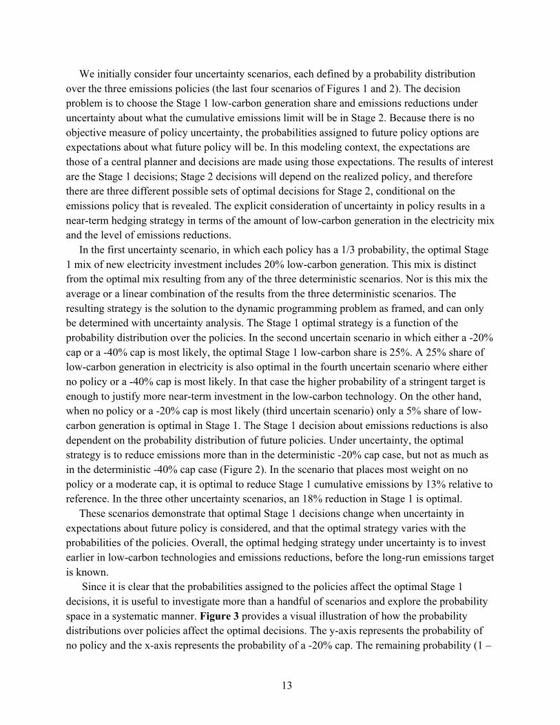
The results of interest from this model are the optimal near-term decisions about new electricity investment shares and emissions reductions under different scenarios of uncertainty in

11

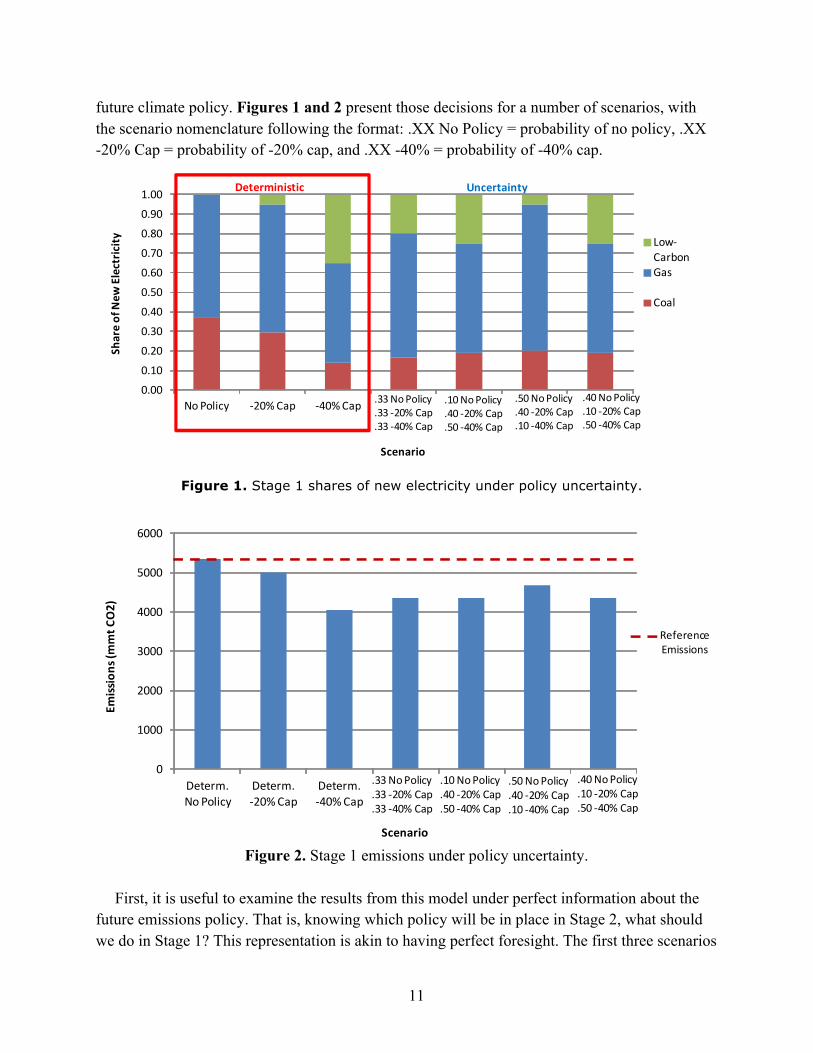
future climate policy. Figures 1 and 2 present those decisions for a number of scenarios, with the scenario nomenclature following the format: .XX No Policy = probability of no policy, .XX -20% Cap = probability of -20% cap, and .XX -40% = probability of -40% cap.

Figure 1. Stage 1 shares of new electricity under policy uncertainty.

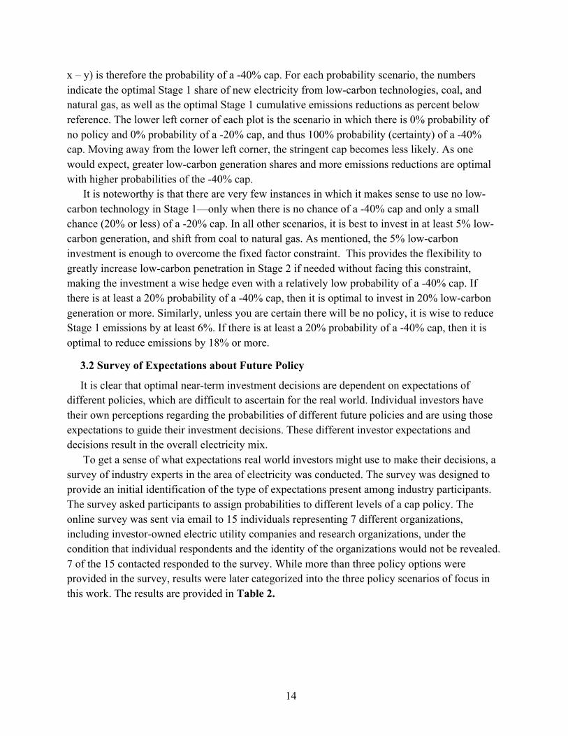
Figure 2. Stage 1 emissions under policy uncertainty. First, it is useful to examine the results from this model under perfect information about the

future emissions policy. That is, knowing which policy will be in place in Stage 2, what should we do in Stage 1? This representation is akin to having perfect foresight. The first three scenarios

0.00

0.10

0.20

0.30

0.40

0.50

0.60

0.70

0.80

0.90

1.00

No  Policy -­‐20%  Cap -­‐40%  Cap

Share  of  New

 Electric

ity

Scenario

Low-­‐CarbonGas

Coal

Uncertainty

.33  No  Policy

.33  -­‐20%  Cap

.33  -­‐40%  Cap

.10  No  Policy

.40  -­‐20%  Cap

.50  -­‐40%  Cap

.50  No  Policy

.40  -­‐20%  Cap

.10  -­‐40%  Cap

.40  No  Policy

.10  -­‐20%  Cap

.50  -­‐40%  Cap

Deterministic

0

1000

2000

3000

4000

5000

6000

Determ.          No  Policy

Determ.              -­‐20%  Cap

Determ.              -­‐40%  Cap

Emissions  (m

mt  C

O2)

Scenario

.33  No  Policy

.33  -­‐20%  Cap

.33  -­‐40%  Cap

.50  No  Policy

.40  -­‐20%  Cap

.10  -­‐40%  Cap

ReferenceEmissions

.10  No  Policy

.40  -­‐20%  Cap

.50  -­‐40%  Cap

.40  No  Policy

.10  -­‐20%  Cap

.50  -­‐40%  Cap

12

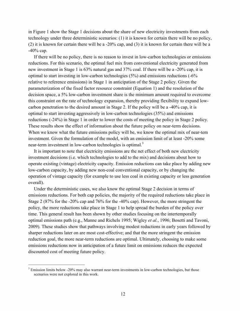
in Figure 1 show the Stage 1 decisions about the share of new electricity investments from each technology under three deterministic scenarios: (1) it is known for certain there will be no policy, (2) it is known for certain there will be a -20% cap, and (3) it is known for certain there will be a -40% cap.

If there will be no policy, there is no reason to invest in low-carbon technologies or emissions reductions. For this scenario, the optimal fuel mix from conventional electricity generated from new investment in Stage 1 is 63% natural gas and 37% coal. If there will be a -20% cap, it is optimal to start investing in low-carbon technologies (5%) and emissions reductions (-6% relative to reference emissions) in Stage 1 in anticipation of the Stage 2 policy. Given the parameterization of the fixed factor resource constraint (Equation 1) and the resolution of the decision space, a 5% low-carbon investment share is the minimum amount required to overcome this constraint on the rate of technology expansion, thereby providing flexibility to expand low-carbon penetration to the desired amount in Stage 2. If the policy will be a -40% cap, it is optimal to start investing aggressively in low-carbon technologies (35%) and emissions reductions (-24%) in Stage 1 in order to lower the costs of meeting the policy in Stage 2 policy. These results show the effect of information about the future policy on near-term decisions. When we know what the future emissions policy will be, we know the optimal mix of near-tem investment. Given the formulation of the model, with an emission limit of at least -20% some near-term investment in low-carbon technologies is optimal.3

It is important to note that electricity emissions are the net effect of both new electricity investment decisions (i.e. which technologies to add to the mix) and decisions about how to operate existing (vintage) electricity capacity. Emission reductions can take place by adding new low-carbon capacity, by adding new non-coal conventional capacity, or by changing the operation of vintage capacity (for example to use less coal in existing capacity or less generation overall).

Under the deterministic cases, we also know the optimal Stage 2 decision in terms of emissions reductions. For both cap policies, the majority of the required reductions take place in Stage 2 (87% for the -20% cap and 76% for the -40% cap). However, the more stringent the policy, the more reductions take place in Stage 1 to help spread the burden of the policy over time. This general result has been shown by other studies focusing on the intertemporally optimal emissions path (e.g., Manne and Richels 1995; Wigley et al., 1996; Bosetti and Tavoni, 2009). These studies show that pathways involving modest reductions in early years followed by sharper reductions later on are most cost-effective; and that the more stringent the emission reduction goal, the more near-term reductions are optimal. Ultimately, choosing to make some emissions reductions now in anticipation of a future limit on emissions reduces the expected discounted cost of meeting future policy.

3 Emission limits below -20% may also warrant near-term investments in low-carbon technologies, but those

scenarios were not explored in this work.

13

We initially consider four uncertainty scenarios, each defined by a probability distribution over the three emissions policies (the last four scenarios of Figures 1 and 2). The decision problem is to choose the Stage 1 low-carbon generation share and emissions reductions under uncertainty about what the cumulative emissions limit will be in Stage 2. Because there is no objective measure of policy uncertainty, the probabilities assigned to future policy options are expectations about what future policy will be. In this modeling context, the expectations are those of a central planner and decisions are made using those expectations. The results of interest are the Stage 1 decisions; Stage 2 decisions will depend on the realized policy, and therefore there are three different possible sets of optimal decisions for Stage 2, conditional on the emissions policy that is revealed. The explicit consideration of uncertainty in policy results in a near-term hedging strategy in terms of the amount of low-carbon generation in the electricity mix and the level of emissions reductions.

In the first uncertainty scenario, in which each policy has a 1/3 probability, the optimal Stage 1 mix of new electricity investment includes 20% low-carbon generation. This mix is distinct from the optimal mix resulting from any of the three deterministic scenarios. Nor is this mix the average or a linear combination of the results from the three deterministic scenarios. The resulting strategy is the solution to the dynamic programming problem as framed, and can only be determined with uncertainty analysis. The Stage 1 optimal strategy is a function of the probability distribution over the policies. In the second uncertain scenario in which either a -20% cap or a -40% cap is most likely, the optimal Stage 1 low-carbon share is 25%. A 25% share of low-carbon generation in electricity is also optimal in the fourth uncertain scenario where either no policy or a -40% cap is most likely. In that case the higher probability of a stringent target is enough to justify more near-term investment in the low-carbon technology. On the other hand, when no policy or a -20% cap is most likely (third uncertain scenario) only a 5% share of low-carbon generation is optimal in Stage 1. The Stage 1 decision about emissions reductions is also dependent on the probability distribution of future policies. Under uncertainty, the optimal strategy is to reduce emissions more than in the deterministic -20% cap case, but not as much as in the deterministic -40% cap case (Figure 2). In the scenario that places most weight on no policy or a moderate cap, it is optimal to reduce Stage 1 cumulative emissions by 13% relative to reference. In the three other uncertainty scenarios, an 18% reduction in Stage 1 is optimal.

These scenarios demonstrate that optimal Stage 1 decisions change when uncertainty in expectations about future policy is considered, and that the optimal strategy varies with the probabilities of the policies. Overall, the optimal hedging strategy under uncertainty is to invest earlier in low-carbon technologies and emissions reductions, before the long-run emissions target is known.

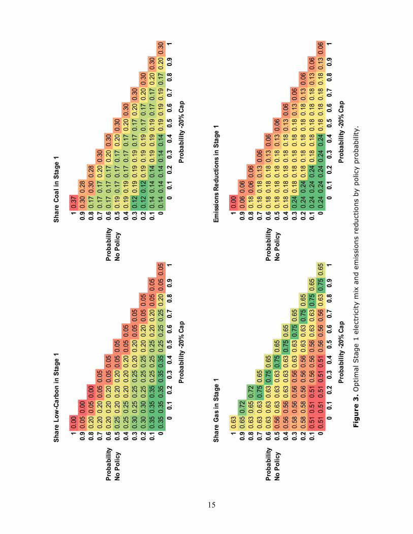
Since it is clear that the probabilities assigned to the policies affect the optimal Stage 1 decisions, it is useful to investigate more than a handful of scenarios and explore the probability space in a systematic manner. Figure 3 provides a visual illustration of how the probability distributions over policies affect the optimal decisions. The y-axis represents the probability of no policy and the x-axis represents the probability of a -20% cap. The remaining probability (1 –

14

x – y) is therefore the probability of a -40% cap. For each probability scenario, the numbers indicate the optimal Stage 1 share of new electricity from low-carbon technologies, coal, and natural gas, as well as the optimal Stage 1 cumulative emissions reductions as percent below reference. The lower left corner of each plot is the scenario in which there is 0% probability of no policy and 0% probability of a -20% cap, and thus 100% probability (certainty) of a -40% cap. Moving away from the lower left corner, the stringent cap becomes less likely. As one would expect, greater low-carbon generation shares and more emissions reductions are optimal with higher probabilities of the -40% cap.

It is noteworthy is that there are very few instances in which it makes sense to use no low-carbon technology in Stage 1—only when there is no chance of a -40% cap and only a small chance (20% or less) of a -20% cap. In all other scenarios, it is best to invest in at least 5% low-carbon generation, and shift from coal to natural gas. As mentioned, the 5% low-carbon investment is enough to overcome the fixed factor constraint. This provides the flexibility to greatly increase low-carbon penetration in Stage 2 if needed without facing this constraint, making the investment a wise hedge even with a relatively low probability of a -40% cap. If there is at least a 20% probability of a -40% cap, then it is optimal to invest in 20% low-carbon generation or more. Similarly, unless you are certain there will be no policy, it is wise to reduce Stage 1 emissions by at least 6%. If there is at least a 20% probability of a -40% cap, then it is optimal to reduce emissions by 18% or more.

3.2 Survey of Expectations about Future Policy

It is clear that optimal near-term investment decisions are dependent on expectations of different policies, which are difficult to ascertain for the real world. Individual investors have their own perceptions regarding the probabilities of different future policies and are using those expectations to guide their investment decisions. These different investor expectations and decisions result in the overall electricity mix.

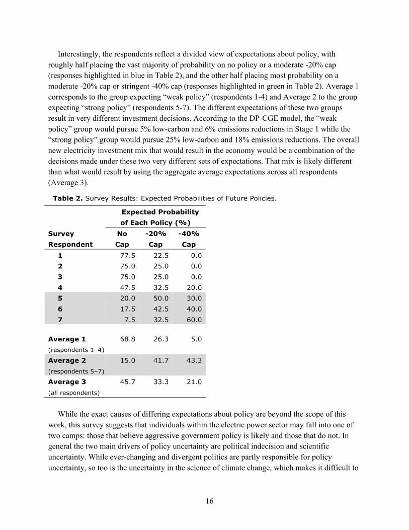
To get a sense of what expectations real world investors might use to make their decisions, a survey of industry experts in the area of electricity was conducted. The survey was designed to provide an initial identification of the type of expectations present among industry participants. The survey asked participants to assign probabilities to different levels of a cap policy. The online survey was sent via email to 15 individuals representing 7 different organizations, including investor-owned electric utility companies and research organizations, under the condition that individual respondents and the identity of the organizations would not be revealed. 7 of the 15 contacted responded to the survey. While more than three policy options were provided in the survey, results were later categorized into the three policy scenarios of focus in this work. The results are provided in Table 2.

15

Fig

ure

3.

Opt

imal

Sta

ge 1

ele

ctri

city

mix

and

em

issi

ons

redu

ctio

ns b

y po

licy

prob

abili

ty.

Shar

e Lo

w-C

arbo

n in

Sta

ge 1

Shar

e Co

al in

Sta

ge 1

10.

001

0.37

0.9

0.05

0.00

0.9

0.30

0.28

0.8

0.20

0.05

0.00

0.8

0.17

0.30

0.28

0.7

0.20

0.20

0.05

0.05

0.7

0.17

0.17

0.20

0.30

Prob

abili

ty

0.6

0.20

0.20

0.20

0.05

0.05

Prob

abili

ty

0.6

0.17

0.17

0.17

0.20

0.30

No P

olic

y0.

50.

250.

200.

200.

200.

050.

05No

Pol

icy

0.5

0.19

0.17

0.17

0.17

0.20

0.30

0.4

0.25

0.25

0.20

0.20

0.20

0.05

0.05

0.4

0.19

0.19

0.17

0.17

0.17

0.20

0.30

0.3

0.30

0.25

0.25

0.25

0.20

0.20

0.05

0.05

0.3

0.12

0.19

0.19

0.19

0.17

0.17

0.20

0.30

0.2

0.30

0.30

0.25

0.25

0.25

0.20

0.20

0.05

0.05

0.2

0.12

0.12

0.19

0.19

0.19

0.17

0.17

0.20

0.30

0.1

0.35

0.35

0.35

0.25

0.25

0.25

0.20

0.20

0.05

0.05

0.1

0.14

0.14

0.14

0.19

0.19

0.19

0.17

0.17

0.20

0.30

00.

350.

350.

350.

350.

350.

250.

250.

250.

200.

050.

050

0.14

0.14

0.14

0.14

0.14

0.19

0.19

0.19

0.17

0.20

0.30

00.

10.

20.

30.

40.

50.

60.

70.

80.

91

00.

10.

20.

30.

40.

50.

60.

70.

80.

91

Prob

abili

ty -2

0% C

apPr

obab

ility

-20%

Cap

Shar

e G

as in

Sta

ge 1

Emis

sion

s Re

duct

ions

in S

tage

1

10.

631

0.00

0.9

0.65

0.72

0.9

0.06

0.06

0.8

0.63

0.65

0.72

0.8

0.18

0.06

0.06

0.7

0.63

0.63

0.75

0.65

0.7

0.18

0.18

0.13

0.06

Prob

abili

ty

0.6

0.63

0.63

0.63

0.75

0.65

Prob

abili

ty

0.6

0.18

0.18

0.18

0.13

0.06

No P

olic

y0.

50.

560.

630.

630.

630.

750.

65No

Pol

icy

0.5

0.18

0.18

0.18

0.18

0.13

0.06

0.4

0.56

0.56

0.63

0.63

0.63

0.75

0.65

0.4

0.18

0.18

0.18

0.18

0.18

0.13

0.06

0.3

0.58

0.56

0.56

0.56

0.63

0.63

0.75

0.65

0.3

0.24

0.18

0.18

0.18

0.18

0.18

0.13

0.06

0.2

0.58

0.58

0.56

0.56

0.56

0.63

0.63

0.75

0.65

0.2

0.24

0.24

0.18

0.18

0.18

0.18

0.18

0.13

0.06

0.1

0.51

0.51

0.51

0.56

0.56

0.56

0.63

0.63

0.75

0.65

0.1

0.24

0.24

0.24

0.18

0.18

0.18

0.18

0.18

0.13

0.06

00.

510.

510.

510.

510.

510.

560.

560.

560.

630.

750.

650

0.24

0.24

0.24

0.24

0.24

0.18

0.18

0.18

0.18

0.13

0.06

00.

10.

20.

30.

40.

50.

60.

70.

80.

91

00.

10.

20.

30.

40.

50.

60.

70.

80.

91

Prob

abili

ty -2

0% C

apPr

obab

ility

-20%

Cap

16

Interestingly, the respondents reflect a divided view of expectations about policy, with roughly half placing the vast majority of probability on no policy or a moderate -20% cap (responses highlighted in blue in Table 2), and the other half placing most probability on a moderate -20% cap or stringent -40% cap (responses highlighted in green in Table 2). Average 1 corresponds to the group expecting “weak policy” (respondents 1-4) and Average 2 to the group expecting “strong policy” (respondents 5-7). The different expectations of these two groups result in very different investment decisions. According to the DP-CGE model, the “weak policy” group would pursue 5% low-carbon and 6% emissions reductions in Stage 1 while the “strong policy” group would pursue 25% low-carbon and 18% emissions reductions. The overall new electricity investment mix that would result in the economy would be a combination of the decisions made under these two very different sets of expectations. That mix is likely different than what would result by using the aggregate average expectations across all respondents (Average 3).

Table 2. Survey Results: Expected Probabilities of Future Policies.

Expected Probability of Each Policy (%)

Survey Respondent

No Cap

-20% Cap

-40% Cap

1 77.5 22.5 0.0 2 75.0 25.0 0.0 3 75.0 25.0 0.0 4 47.5 32.5 20.0 5 20.0 50.0 30.0 6 17.5 42.5 40.0 7 7.5 32.5 60.0

Average 1 68.8 26.3 5.0 (respondents 1–4)

Average 2 15.0 41.7 43.3 (respondents 5–7)

Average 3 45.7 33.3 21.0 (all respondents)

While the exact causes of differing expectations about policy are beyond the scope of this

work, this survey suggests that individuals within the electric power sector may fall into one of two camps: those that believe aggressive government policy is likely and those that do not. In general the two main drivers of policy uncertainty are political indecision and scientific uncertainty. While ever-changing and divergent politics are partly responsible for policy uncertainty, so too is the uncertainty in the science of climate change, which makes it difficult to

17

determine the level of emissions reduction action that should be taken. Those within the “weak policy” group may expect political gridlock, future political leadership that is not in favor of climate policy, unresolved climate science that prevents action, or climate science suggesting that climate change is not a severe problem. On the other hand, those within the “strong policy” group may expect future political leadership that is in favor of climate policy or climate science demonstrating that climate change is a severe problem that requires aggressive action to address.

Regardless of the causes, this divided view has implications for policy and modeling. It indicates the difficulty of building consensus on future policy. Different investment strategies today mean that companies that guess correctly about the future policy environment will profit or be in a better position in the future, while those who guess wrong will lose or be worse off in the future. Recognizing this, companies would have an incentive to try to affect the future policy outcome to avoid being on the losing side. These differing views and goals may result in a political economy in which consensus on climate policy is difficult. This is problematic because, as the following section shows, policy uncertainty can be costly, meaning that consensus is valuable.

Further, from a CGE modeling perspective this divided view suggests the potential value of representing multiple representative agents with different expectations and utility functions in future work. This would enable study of how policy impacts agents differently, as well as how the investments made by those with divergent expectations differ from those made from the perspective of a central planner.

3.3 Effects of Uncertainty

3.3.1 The Cost of Uncertainty in Policy Using the DP-CGE model we can estimate the economy-wide cost of policies as well as the

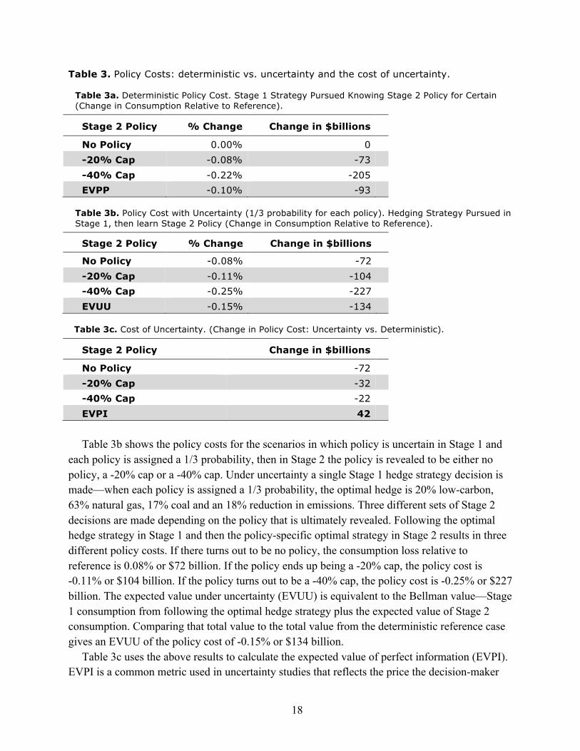
cost of uncertainty in the policy (the cost borne as a direct result of the policy uncertainty, which is additional to the cost of meeting the cap). The top two sections of Table 3 show the policy costs in terms of change in cumulative economy-wide consumption relative to the reference no policy case. The cost is shown both as a percentage change and in billions of dollars. The top section shows these costs for the deterministic scenarios in which there is perfect information in Stage 1 as to what the Stage 2 policy will be. In that case, the -20% cap results in a consumption loss of -0.08% or $73 billion, and the -40% cap results in a loss of -0.22% or $205 billion. We can then calculate the expected value using a perfect prediction (EVPP) by assigning probabilities to which policy will be known for certain and taking the expected value (see Equation 3). For example, assume a 33% chance that in Stage 1 we will know for certain there will be no policy, a 33% chance we will know for certain there will be a -20% cap, and a 33% chance we will know for certain there will be a -40% cap (i.e. p1=p2=p3=1/3). In that case, EVPP of the policy cost is -0.10% or $93 billion.

EVPP = p1*(cost when certain no policy) + p2*(cost when certain -20% cap) (3)

+ p3*(cost when certain -40% cap)

18

Table 3. Policy Costs: deterministic vs. uncertainty and the cost of uncertainty.

Table 3a. Deterministic Policy Cost. Stage 1 Strategy Pursued Knowing Stage 2 Policy for Certain (Change in Consumption Relative to Reference).

Stage 2 Policy % Change Change in $billions

No Policy 0.00% 0 -20% Cap -0.08% -73 -40% Cap -0.22% -205 EVPP -0.10% -93

Table 3b. Policy Cost with Uncertainty (1/3 probability for each policy). Hedging Strategy Pursued in Stage 1, then learn Stage 2 Policy (Change in Consumption Relative to Reference).

Stage 2 Policy % Change Change in $billions

No Policy -0.08% -72 -20% Cap -0.11% -104 -40% Cap -0.25% -227 EVUU -0.15% -134

Table 3c. Cost of Uncertainty. (Change in Policy Cost: Uncertainty vs. Deterministic).

Stage 2 Policy Change in $billions

No Policy -72 -20% Cap -32 -40% Cap -22 EVPI 42 Table 3b shows the policy costs for the scenarios in which policy is uncertain in Stage 1 and

each policy is assigned a 1/3 probability, then in Stage 2 the policy is revealed to be either no policy, a -20% cap or a -40% cap. Under uncertainty a single Stage 1 hedge strategy decision is made—when each policy is assigned a 1/3 probability, the optimal hedge is 20% low-carbon, 63% natural gas, 17% coal and an 18% reduction in emissions. Three different sets of Stage 2 decisions are made depending on the policy that is ultimately revealed. Following the optimal hedge strategy in Stage 1 and then the policy-specific optimal strategy in Stage 2 results in three different policy costs. If there turns out to be no policy, the consumption loss relative to reference is 0.08% or $72 billion. If the policy ends up being a -20% cap, the policy cost is -0.11% or $104 billion. If the policy turns out to be a -40% cap, the policy cost is -0.25% or $227 billion. The expected value under uncertainty (EVUU) is equivalent to the Bellman value—Stage 1 consumption from following the optimal hedge strategy plus the expected value of Stage 2 consumption. Comparing that total value to the total value from the deterministic reference case gives an EVUU of the policy cost of -0.15% or $134 billion.

Table 3c uses the above results to calculate the expected value of perfect information (EVPI). EVPI is a common metric used in uncertainty studies that reflects the price the decision-maker

19

would be willing to pay in order to gain access to perfect information. It is defined as the difference between EVPP and EVUU. The inverse of EVPI is the expected cost of uncertainty— the additional policy cost expected to be borne as a direct result of uncertainty in the policy. We can think of this as the cost of political indecision or of missing information. If the cumulative emissions limit was chosen and known in advance, optimal investment and emissions decisions could be made anticipating that policy. When the policy is uncertain, the best we can do in Stage 1 is to pursue the optimal hedging strategy. In this case, EVPI, and hence the cost of policy uncertainty, is $42 billion. Uncertainty increases the expected cost of policy by over 45%.

These results demonstrate that uncertainty in the policy is a real added cost—increasing the expected cost of policy by over 45%. Even while pursuing the optimal hedging strategy under uncertainty, once the policy is known, those hedging decisions are not necessarily optimal in retrospect. This suggests the value of setting clear, long-term policies so that decisions can be made with more complete information.

Table 3c also shows the added cost of uncertainty for each of the three policies, comparing consumption loss in the scenarios with uncertainty to the deterministic scenarios. These results drive the EVPI. If no policy is implemented, uncertainty costs an additional $72 billion. This is because the optimal hedge strategy pursued expensive low-carbon technology and emissions reduction investments that turned out to be unnecessary in the absence of policy. If a -20% cap is implemented, uncertainty costs an additional $32 billion, reducing consumption by 43% compared to when the policy is certain. In this case, the hedging strategy also overinvested in low-carbon generation and emissions reductions relative to what was required to meet the -20% cap. If it was known ahead of time that the policy would be a -20% cap, it would have been best to pursue 5% low-carbon generation (instead of 20%) and 6% reductions (instead of 18%) in Stage 1. If a -40% cap is implemented, uncertainty costs an additional $22 billion, reducing consumption by 11% compared to when the policy is certain. In this case the hedging strategy underinvested in low-carbon generation and emissions reductions and overinvested in conventional technologies. If it had been known ahead of time that the policy would be a -40% cap, it would have been best to pursue 35% low-carbon generation (instead of 20%), 51% natural gas (instead of 63%), 14% coal (instead of 17%) and 24% reductions (instead of 18%) in Stage 1. The cost of the uncertainty in this case is mainly driven by the overinvestment in conventional generation capacity which cannot be fully utilized in Stage 2 due to the stringent emissions constraint. It is very expensive to leave existing (vintage) capacity unused or underutilized.

The results above suggest a cost asymmetry between overinvesting in conventional generation and overinvesting in low-carbon generation. To investigate this asymmetry further, we consider two extreme cases: (1) it is assumed with certainty that there will be no policy, but there turns out to be a -40% cap, and (2) it is assumed with certainty that there will be a -40% cap, but there turns out to be no policy. In the first case, the policy cost of meeting the -40% cap is very high—2.3%. This high cost is due to an overinvestment in conventional generation. All Stage 1 investment is in conventional generation, and then in Stage 2, in order to meet the policy, new investment must be 50% low-carbon generation and almost 60% of existing vintage conventional

20

generation must be left unused (stranded). The amount of stranded vintage capital is calculated by tracking in the model the total amount of generation capacity of each type available and the total amount actually used in electricity generation, the difference is available capacity that is left stranded. Leaving 60% of available conventional generation capital unused indicates poor near-term investment decisions.

In the second case, the consumption loss for overinvesting in low-carbon generation is 0.13%. Although the low-carbon generation turned out to be unnecessary in the absence of policy, none of the vintage low-carbon capacity goes unused. This asymmetry is driven by the variable costs of operating. With an emissions limit, the carbon price increases the fuel cost component of conventional (fossil) generation. Even though the capital investment is sunk, the variable cost of operating the conventional generation (mainly the fuel cost) is greater than the full cost of investing in new low-carbon generation. As a result, vintage conventional generation capacity is left unused. On the other hand, low-carbon generation has low variable costs (and no fuel costs), so once the capital investment is made, operation is relatively inexpensive, and lower than the full cost of investing in new conventional generation. As a result, vintage low-carbon capacity continues to be used even when there is no policy. This cost asymmetry suggests that in making investment decisions it may be wise to err on the side of too much low-carbon generation instead of too much conventional generation.

3.3.2 The Value of Including Uncertainty One of the contributions of this research is demonstrating how decision-making under

uncertainty can be represented in a CGE model and the value of doing so. The expected value of including uncertainty (EVIU) is a metric that captures the value of representing uncertainty or, conversely, the additional cost of assuming certainty. EVIU reflects the improvement in decisions obtained from explicitly representing uncertainty in the decision-making process. To demonstrate the value of including uncertainty, consider six Stage 1 strategies: (1) the optimal strategy from the DP-CGE model assuming 1/3 probability for each policy, (2) the “average” strategy—the expected value of the uncertain cap level (i.e. -20% cap) is imposed as though it is certain, (3) the myopic strategy (i.e. no investments in low-carbon technologies or emissions reductions until the policy is known), and (4–6) the three perfect foresight strategies- one for each of the three policies when assumed to be certain. For each of these Stage 1 strategies, the best Stage 2 strategy for each of the three possible emissions limits is identified. The expected policy cost is then calculated assuming each policy outcome is equally likely.

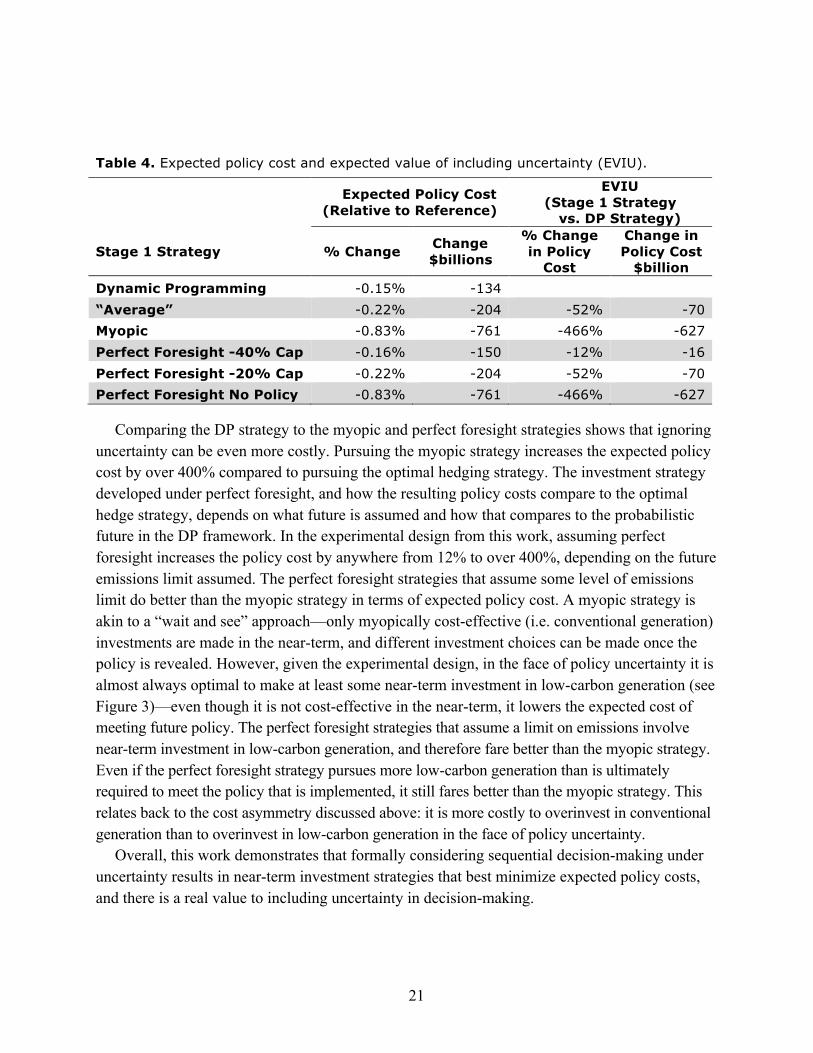
Table 4 compares the expected policy costs for the six Stage 1 strategies, and shows that the DP strategy is the best (has the lowest expected policy cost) in the face of uncertainty. The EVIU is calculated by comparing policy costs from each strategy to those from the DP strategy. The EVIU compared to the “average” strategy is $70 billion. It is the mistake of the flaw of averages to assume the average of the scenarios would make the best strategy. In this case, doing so increases the expected policy cost by over 50% compared to pursuing the optimal hedging strategy.

21

Table 4. Expected policy cost and expected value of including uncertainty (EVIU).

Expected Policy Cost (Relative to Reference)

EVIU (Stage 1 Strategy

vs. DP Strategy)

Stage 1 Strategy % Change Change $billions

% Change in Policy

Cost

Change in Policy Cost

$billion Dynamic Programming -0.15% -134 “Average” -0.22% -204 -52% -70 Myopic -0.83% -761 -466% -627 Perfect Foresight -40% Cap -0.16% -150 -12% -16 Perfect Foresight -20% Cap -0.22% -204 -52% -70 Perfect Foresight No Policy -0.83% -761 -466% -627

Comparing the DP strategy to the myopic and perfect foresight strategies shows that ignoring uncertainty can be even more costly. Pursuing the myopic strategy increases the expected policy cost by over 400% compared to pursuing the optimal hedging strategy. The investment strategy developed under perfect foresight, and how the resulting policy costs compare to the optimal hedge strategy, depends on what future is assumed and how that compares to the probabilistic future in the DP framework. In the experimental design from this work, assuming perfect foresight increases the policy cost by anywhere from 12% to over 400%, depending on the future emissions limit assumed. The perfect foresight strategies that assume some level of emissions limit do better than the myopic strategy in terms of expected policy cost. A myopic strategy is akin to a “wait and see” approach—only myopically cost-effective (i.e. conventional generation) investments are made in the near-term, and different investment choices can be made once the policy is revealed. However, given the experimental design, in the face of policy uncertainty it is almost always optimal to make at least some near-term investment in low-carbon generation (see Figure 3)—even though it is not cost-effective in the near-term, it lowers the expected cost of meeting future policy. The perfect foresight strategies that assume a limit on emissions involve near-term investment in low-carbon generation, and therefore fare better than the myopic strategy. Even if the perfect foresight strategy pursues more low-carbon generation than is ultimately required to meet the policy that is implemented, it still fares better than the myopic strategy. This relates back to the cost asymmetry discussed above: it is more costly to overinvest in conventional generation than to overinvest in low-carbon generation in the face of policy uncertainty.

Overall, this work demonstrates that formally considering sequential decision-making under uncertainty results in near-term investment strategies that best minimize expected policy costs, and there is a real value to including uncertainty in decision-making.

22

4. SENSITIVITY TO LIMITS ON LOW-CARBON GENERATION GROWTH RATES

In the above results, the rate of low-carbon generation expansion is limited by the availability of fixed factor resource (see Equation 1). This is a critical parameter because when a substantial amount of low-carbon generation is needed in Stage 2 it creates a strong incentive to develop the technology in Stage 1. As seen from the results, the formulation of the fixed factor expansion means that as long as ~5% of investment in Stage 1 is in low-carbon generation then low-carbon generation is not significantly limited in Stage 2. To further investigate the sensitivity of results to low-carbon generation expansion rates, an alternative formulation is developed in which the low-carbon generation share in Stage 2 is strictly limited depending on the share in Stage 1. This exogenous low-carbon generation growth rate limit overrides the fixed factor.

This additional constraint limits the rate of growth of low-carbon generation as a share of new electricity between Stage 1 and Stage 2. All of the results presented in the previous sections assumed that the share of low-carbon generation cannot increase by more than 50 percentage points from Stage 1 to Stage 2. So if the share was 0% in Stage 1, the most it could be in Stage 2 is 50%. If the share was 20% in Stage 1, the most it could be in Stage 2 is 70%. It is possible that there is no limit on how much the share of low-carbon generation grows—low-carbon could constitute 0% of new electricity in Stage 1 and 100% in Stage 2. This would reflect that all new generation capacity put in place from 2021 to 2030 is low-carbon. While theoretically possible, such a solution does not seem likely or technologically feasible. All investors would have to decide to build low-carbon capacity, an unlikely prospect. Further, engineering and operational constraints (e.g., transmission constraints, reliability issues, etc.) would have to be overcome in a very short period of time in order for the electricity system to handle such large low-carbon capacity additions. However, in the past we have seen rather rapid expansion of nuclear electricity, and currently natural gas generation is quickly expanding due to the success of shale gas driving down fuel prices, suggesting there may not be much of a limit to the rate of low-carbon growth. Because it is difficult to assess and people have very different opinions about what type of low-carbon growth rate is realistic from an engineering and technological standpoint, this section conducts sensitivity analysis on the limit to low-carbon growth rates.

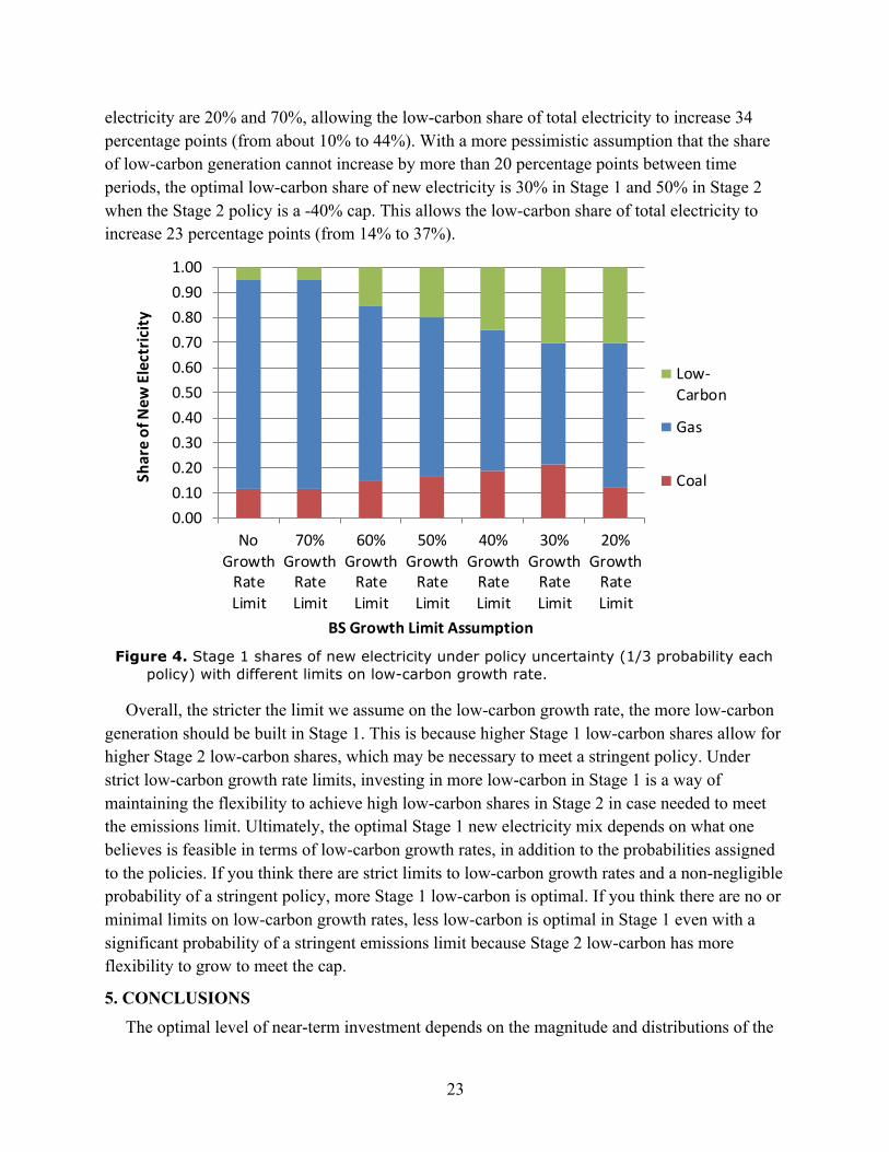
Figure 4 illustrates the impact of the low-carbon growth rate limit assumption on the optimal Stage 1 new electricity mix when there is a 1/3 probability of each policy. If there is no limit on how much the share of low-carbon can grow, the optimal Stage 1 strategy involves 5% low-carbon generation. If the policy ends up being a -40% cap, the optimal Stage 2 low-carbon share is then 80%. That is an increase of 75 percentage points in the low-carbon share of new electricity. In terms of share of total electricity (not just new electricity), low-carbon in this case increases 41 percentage points (from under 3% to almost 44%) in just ten years, reflecting a drastic change to the electricity sector in a very short period of time (particularly considering total electricity demand is growing over time). A change like this is questionable from a practical engineering standpoint. The base assumption that the share of low-carbon generation cannot increase by more than 50 percentage points between time periods is still optimistic. When the Stage 2 policy is a -40% cap, the optimal Stage 1 and Stage 2 low-carbon shares of new

23

electricity are 20% and 70%, allowing the low-carbon share of total electricity to increase 34 percentage points (from about 10% to 44%). With a more pessimistic assumption that the share of low-carbon generation cannot increase by more than 20 percentage points between time periods, the optimal low-carbon share of new electricity is 30% in Stage 1 and 50% in Stage 2 when the Stage 2 policy is a -40% cap. This allows the low-carbon share of total electricity to increase 23 percentage points (from 14% to 37%).

Figure 4. Stage 1 shares of new electricity under policy uncertainty (1/3 probability each policy) with different limits on low-carbon growth rate.

Overall, the stricter the limit we assume on the low-carbon growth rate, the more low-carbon generation should be built in Stage 1. This is because higher Stage 1 low-carbon shares allow for higher Stage 2 low-carbon shares, which may be necessary to meet a stringent policy. Under strict low-carbon growth rate limits, investing in more low-carbon in Stage 1 is a way of maintaining the flexibility to achieve high low-carbon shares in Stage 2 in case needed to meet the emissions limit. Ultimately, the optimal Stage 1 new electricity mix depends on what one believes is feasible in terms of low-carbon growth rates, in addition to the probabilities assigned to the policies. If you think there are strict limits to low-carbon growth rates and a non-negligible probability of a stringent policy, more Stage 1 low-carbon is optimal. If you think there are no or minimal limits on low-carbon growth rates, less low-carbon is optimal in Stage 1 even with a significant probability of a stringent emissions limit because Stage 2 low-carbon has more flexibility to grow to meet the cap.

5. CONCLUSIONS

The optimal level of near-term investment depends on the magnitude and distributions of the

0.000.100.200.300.400.500.600.700.800.901.00

NoGrowthRateLimit

70%GrowthRateLimit

60%GrowthRateLimit

50%GrowthRateLimit

40%GrowthRateLimit

30%GrowthRateLimit

20%GrowthRateLimit

Share  of  New

 Electric

ity

BS  Growth  Limit  Assumption

Low-­‐Carbon

Gas

Coal

24

uncertainties considered. Uncertainty creates risks, and the best one can do in the face of uncertainty is to develop near-term investment strategies that hedge against those risks. In this work, the two risks considered are: (1) the sunk cost of near-term low-carbon technology investments that prove to be unnecessary, and (2) facing high future policy costs. The first risk is created if near-term investments in expensive low-carbon technologies are made, but ultimately no policy limiting electricity emissions is implemented, or a weak policy is implemented that does not require low-carbon technologies to the extent they were deployed. The second risk is created when future policy requires significant emissions reductions and significant amounts of low-carbon generation, but failure to make (sufficient) near-term investments results in high costs to meet the policy. A carbon-intensive electricity mix combined with low-carbon technologies that may not be able to expand as much as desired leads to high policy costs in that case. How to balance these two risks depends on the perceived probabilities of future outcomes and requires explicit consideration of the uncertainty in the decision-making process. This work shows that there is value to investing in low-carbon generation now and taking on some of the first risk in order to provide flexibility in meeting future policy and reduce the second risk.

This work demonstrates that formally considering uncertainty (and the risks it creates) in the decision-making process results in different near-term decisions than would have been made if the uncertainty were ignored or not truly incorporated into decision-making. Considering decisions under uncertainty results in a hedging strategy: invest in more low-carbon generation now than would be needed for near-term goals alone in order to minimize expected future policy costs. The amount of near-term investment depends on the expectations of future outcomes. More near-term investment should be made as we expect stringent policy to be more likely. As the expected probability of a stringent cap increases, the potential need for significant amounts of low-carbon generation to meet the cap increases, and in turn the value of near-term investments in those technologies increases because they reduce the expected discounted cost of meeting the policy. They do so by developing a less carbon-intensive electricity mix, helping to overcome technology expansion rate constraints, and spreading the burden of emissions reductions over time—all of which provide future flexibility.

Similarly, the stricter the constraints on the rate of technology expansion are, the greater the value of near-term investments. Near-term investments that create the needed infrastructure for commercialization of these new technologies in the present can help limit bottlenecks to greater expansion in the future if it turns out that the policy is stringent enough to require significant use of low-carbon technologies. Factors that may limit the expansion rate of a technology include limited trained engineering capacity and electricity system adjustment costs. Near-term investments could help overcome those limits, providing flexibility to rapidly expand the future use of low-carbon technologies if needed in order to meet a future emissions limit.

Also, this work suggests that overinvestment in conventional technologies poses a greater risk under policy uncertainty than overinvestment in low-carbon technologies due to differences in variable costs. If a stringent policy is implemented, overbuilt conventional capacity may need to be stranded due to high operating costs driven by high fuel costs that reflect the carbon price. If

25

no or weak policy is implemented, overbuilt low-carbon capacity means unnecessary sunk capital costs, but low operating costs allow the capacity to continue to be used.

Overall, more near-term low-carbon investments create future flexibility, which justifies the additional near-term cost of investments. The value of this flexibility is only explicitly considered in the context of decision-making under uncertainty.

This work also shows that uncertainty has a cost, beyond the cost of meeting the policy. In the experimental design used here, uncertainty about the future policy increases the expected discounted cost of policy by over 45%. Even while pursuing the optimal hedging strategy under uncertainty, once the policy is known, those hedge decisions are not necessarily optimal in retrospect. Had the policy been known for certain, different near-term decisions would have been made that would have resulted in lower policy costs. We can think of this as the cost of political indecision and/or of missing scientific information, which are the two main drivers of policy uncertainty. While regularly changing and divergent politics are partly responsible for policy uncertainty, so too is the uncertainty in the science of climate change, which makes it difficult to determine the level of emissions reduction action that should be taken. While these drivers are beyond the scope of this research, the high cost of uncertainty suggests the value of doing what we can to resolve it—in particular, more climate research (to the extent that it can improve our understanding of the severity of the problem) and efforts to develop a political consensus sooner. If consensus can be reached and the science uncertainties resolved, setting clear, long-term policies can minimize expected policy costs. Given the risks associated with climate change as reported in various national and international research assessments, such as the Fourth Assessment Report of the Intergovernmental Panel on Climate Change (IPCC, 2007) and the U.S. Second National Climate Assessment (USGCRP, 2009), it would seem difficult to make the case that no emissions reduction policy is warranted now or in the future.

This work also demonstrates the value of formally representing uncertainty in decision-support models. As noted previously, existing modeling approaches typically do one of two things with regard to uncertainty: (1) ignore it (either by being myopic or pretending we have perfect foresight) or (2) consider scenarios, each with certainty, and then use the middle one or use the average of the uncertain value as though certain. These approaches result in different investment strategies that increase the expected policy cost relative to the optimal hedging strategy from a dynamic programming framework that explicitly considers decision-making under uncertainty. Given the experimental design, the expected policy cost increases over 50% when pursuing an “average” strategy; over 400% when pursuing a myopic strategy; and 12% to over 400% when pursuing a perfect foresight strategy (depending on the future policy assumed). Overall, this work demonstrates that considering uncertainty in decision-making results in investment strategies that best minimize expected policy costs.

The main technical contribution of this work is to provide a new decision-support framework that considers economy-wide effects of electric power sector investment decisions under uncertainty. There have been sector-specific studies that capture decision-making under uncertainty well, but cannot address economy-wide social welfare implications. There have been

26

economy-wide computable general equilibrium (CGE) studies with uncertainty, but without capturing the critical nature making decisions under uncertainty, learning, and then making decisions again. This work makes the unique contribution of modeling decision-making under uncertainty with learning and the ability to revise decisions over time in a framework that represents the entire economy and can measure social welfare impacts. Applying this new modeling approach allows for a quantitative evaluation of near-term electric power investment decisions under uncertainty. In doing so, this work demonstrates how a CGE model can be restructured to capture stochastic dynamic expectations. As a result, this work facilitates further model development and analysis in this area. In addition, the modeling approach developed here can be applied to other sectors, other decisions, and other uncertainties.

Acknowledgments The authors gratefully acknowledge the financial support for this work provided by the U.S. Department of Energy, Office of Science under grants DE-PS02-09ER09-26, DE-FG02-94ER61937, DE-FG02-08ER64597, DE-FG02-93ER61677, DE-SC0003906, DE- SC0007114, XEU-0-9920-01; the U.S. Environmental Protection Agency under grants XA-83240101, PI-83412601-0, RD-83427901-0, XA-83505101-0, XA-83600001-1, and subcontract UTA12-000624; and a consortium of government, industrial and foundation sponsors (for the complete list see: http://globalchange.mit.edu/sponsors/all).

6. REFERENCES Bellman, R.E., 1957: Dynamic Programming. Princeton University Press: Princeton, NJ, Republished

2003: Dover. Bergerson, J.A. and L.B. Lave, 2007: Baseload Coal Investment Decisions under Uncertain Carbon

Legislation. Environmental Science and Technology, 41(10): 3431–3436. Bistline, J.E. and J.P. Weyant, 2013: Electric sector investments under technological and policy-related

uncertainties: a stochastic programming approach. Climatic Change, 121:143–160. Blanford, G.J., 2009: R&D Investment Strategy for Climate Change. Energy Economics, 31: S27–S36,

Supplement 1. Botterud, A., M.D. Ilic and I. Wangernsteen, 2005: Optimal Investments in Power Generation under

Centralized and Decentralized Decision-making. IEEE Transactions on Power Systems, 20(1): 254–263. Bossetti, V. and M. Tavoni, 2009: Uncertain R&D, Backstop Technology, and GHGs Stabilization.

Energy Economics, 31: S18–S26. Clarke, L., J. Edmonds, H. Jacoby, H. Pitcher, J. Reilly, R. Richels, 2007: Scenarios of Greenhouse Gas

Emissions and Atmospheric Concentrations. Sub-report 2.1A of Synthesis and Assessment Product 2.1 by the U.S. Climate Change Science Program and the Subcommittee on Global Change Research, Department of Energy, Office of Biological and Environmental Research: Washington, D.C.

Crost, B. and C. Traeger, 2010: Risk and Aversion in the Integrated Assessment of Climate Change. CUDARE Working Paper No. 1104.

Dimaranan, B. and R. McDougall, 2002: Global Trade, Assistance, and Production: The GTAP 5 Data Base. Center for Global Trade Analysis, Purdue University: West Lafayette, Indiana.

Fisher, B.S., N. Nakicenovic, K. Alfsen, J. Corfee Morlot, F. de la Chesnaye, J.-Ch. Hourcade, K. Jiang, M. Kainuma, E. La Rovere, A. Matysek, A. Rana, K. Riahi, R. Richels, S. Rose, D. van Vuuren and R. Warren, 2007: Issues Related to Mitigation in the Long Term Context. In: Climate Change 2007: Mitigation. Contribution of Working Group III to the Fourth Assessment Report of the Inter-governmental Panel on Climate Change, B. Metz, O.R. Davidson, P.R. Bosch, R. Dave and L.A.

27

Meyer (eds.), Cambridge University Press: Cambridge, U.K. Gerst, M., R. Howarth and M. Borsuk, 2010: Accounting for the risk of extreme outcomes in an

integrated assessment of climate change. Energy Policy, 38(8): 4540–4548. Grubb, M., J. Köhler and D. Anderson, 2002: Induced Technical Change in Energy and Environmental

Modeling: Analytic Approaches and Policy Implications. Annual Review of Energy and the Environment, 27: 271–308.

Grubler, A. and A. Gritsevskii, 1997: A Model of Endogenous Technological Change Through Uncertain Returns on Learning (R&D and investments). Conf. Induc. Technol. Change Environ. International Institute of Applied System Analysis, Laxenburg, Austria.

Hammitt, J.K., R.A. Lempert and M.E. Schlesinger, 1992: A Sequential-Decision Strategy for Abating Climate Change. Nature, 357(6376): 315–318.

Hertel, T., 1997: Global Trade Analysis: Modeling and Applications. Cambridge University Press: Cambridge, UK.

IPCC [Intergovernmental Panel on Climate Change], 2007: Climate Change 2007: Impacts, Adaptation and Vulnerability. Contribution of Working Group II to the Fourth Assessment Report of the Intergovernmental Panel on Climate Change, Cambridge University Press: Cambridge, UK.

Jacoby, H.D., J.M. Reilly, J.R. McFarland and S. Paltsev (2006). Technology and Technical Change in the MIT EPPA Model. Energy Economics, 28(5-6): 610-631.

Kelly, D. and C. Kolstad, 1999: Bayesian Learning, Growth, and Pollution. Journal of Economic Dynamics and Control, 23(4): 491–518.

Klein, A., J. Bouchard, and S. Goutier, 2008: Generation Capacity Expansion under Long-Term Uncertainties in the U.S. Electric Market. United States Association of Energy Economics Conference Paper.

Kolstad, C.D., 1996: Learning and Stock Effects in Environmental Regulation: The Case of Greenhouse Gas Emissions. Journal of Environmental Economics and Management, 31(1): 1–18.

Kypreos, S. and L. Barreto, 2000: ERIS: A Model Prototype with Endogenous Technological Change. International Journal of Global Energy Issues, 14(1–4): 374–396.

Lemoine, D. and C. Traeger, 2011: Tipping Points and Ambiguity in the Integrated Assessment of Climate Change. NBER Environmental and Energy Economics Summer Institute Paper.

Manne, A.S. and R.G. Richels, 1995: The Greenhouse Debate: Economic Efficiency, Burden Sharing and Hedging Strategies. The Energy Journal, 16(4): 1–37.

Manne, A.S. and R.G. Richels, 1994: The Costs of Stabilizing Global CO2 Emissions: A Probabilistic Analysis Based on Expert Judgment. The Energy Journal, 15(1): 31–56.

Mattsson, N., 2002: Introducing Uncertain Learning in an Energy System Model: A Pilot Study Using GENIE. International Journal of Global Energy Issues, 18(2/3/4): 253–265.

McFarland, J.R., J.M. Reilly and H.J. Herzog, 2004: Representing Energy Technologies in Top-Down Economic Models Using Bottom-Up Information. Energy Economics, 26(4): 685–707.

Messner, S., A. Golodnikov and A. Gritsevskii, 1995: A Stochastic Version of the Dynamic Linear Programming Model MESSAGE III. Energy, 21(9): 775–784.

Metcalf, G.E., S. Paltsev, J.M. Reilly, H.D. Jacoby and J. Holak (2008). Analysis of U.S. Greenhouse Gas Tax Proposals. MIT Joint Program on the Science and Policy of Global Change Report 160, (Available at: http://globalchange.mit.edu/files/document/MITJPSPGC_Rpt160.pdf).

Morris, J.F., J.M. Reilly and S. Paltsev (2010). Combining a Renewable Portfolio Standard with a Cap-and-Trade Policy: A General Equilibrium Analysis. MIT Joint Program on the Science and Policy of Global Change Report 187, (Available at: http://globalchange.mit.edu/files/document/MITJPSPGC_Rpt187.pdf).

Nordhaus, W.D. and D. Popp, 1997: What is the Value of Scientific Knowledge? An Application to Global Warming Using the PRICE Model. The Energy Journal, 18(1): 1–45.

28

Paltsev, S., J. M. Reilly, H.D. Jacoby, and J.F Morris, 2009: The Cost of Climate Policy in the United States. MIT JPSPGC Report 173, September, 55 p. (http://globalchange.mit.edu/files/document/MITJPSPGC_Rpt173.pdf).

Paltsev, S., J.M. Reilly, H.D. Jacoby, A.C. Gurgel, G.E. Metcalf, A.P. Sokolov and J.F. Holak, 2008: Assessment of US GHG Cap-and-Trade Proposals. Climate Policy, 8(4): 395–420.

Paltsev, S., J.M. Reilly, H.D. Jacoby, R.S. Eckaus, J. McFarland, M. Sarofim, M. Asadoorian, M. Babiker, 2005: The MIT Emissions Prediction and Policy Analysis (EPPA) Model: Version 4. MIT JPSPGC Report 125, August, 72 p. (http://globalchange.mit.edu/files/document/MITJPSPGC_Rpt125.pdf).

Powell, W.B., A. George, H. Simão, W. Scott, A. Lamont and J. Stewart, 2012: SMART: A Stochastic Multiscale Model for the Analysis of Energy Resources, Technology and Policy. INFORMS Journal on Computing, 24(4): 665–682.

Reilly J.M., J. Melillo, C. Yongxia, D. Kicklighter, A. Gurgel, S. Paltsev, T. Cronin, A.P. Sokolov and A. Schlosser, 2012: Using Land to Mitigate Climate Change: Hitting the Target, Recognizing the Trade-offs. Environmental Science and Technology, 46(11): 5672–5679 (Supporting Information).

Reilly, J.M., J. Edmonds, R. Gardner and A. Brenkert, 1987: Monte Carlo Analysis of the IEA/ORAU Energy/Carbon Emissions Model. The Energy Journal, 8(3): 1–29.

Richels, R.G. and G.J. Blanford, 2008: The Value of Technological Advance in Decarbonizing the U.S. Economy. Energy Economics, 30(6): 2930–2946.

Rutherford, T.F., 1999: Applied General Equilibrium Modeling with MPSGE as a GAMS Subsystem: An Overview of the Modeling Framework and Syntax. Computational Economics, 14: 1–46.

Santen, N.R., 2012: Technology Investment Decisions under Uncertainty: A New Modeling Framework for the Electric Power Sector. Massachusetts Institute of Technology Doctoral Dissertation, Engineering Systems Division.

Scott, M.J., R.D. Sands, J. Edmonds, A.M. Liebetrau and D.W. Engel, 1999: Uncertainty in Integrated Assessment Models: Modeling with MiniCAM 1.0. Energy Policy, 27(14): 597.

USGCRP [U.S. Global Change Research Program], 2009: Global Climate Change Impacts in the United States. Cambridge University Press: New York.

Webster, M.D., 2008: Incorporating Path-Dependency into Decision Analytic Methods: An Application to Global Climate Change Policy. Decision Analysis, 5(2): 60–75.

Webster, M.D., 2002: The Curious Role of Learning: Should We Wait for More Data? The Energy Journal, 23(2): 97–119.

Webster, M.D., A.P. Sokolov, J.M. Reilly, C. Forest, S. Paltsev, C.A. Schlosser, C. Wang, D.W. Kicklighter, M. Sarofim, J.M. Melillo, R.G. Prinn and H.D. Jacoby, 2012: Analysis of climate policy targets under uncertainty. Climatic Change, 112(3–4) 569–583.

Webster, M.D., S. Paltsev, J. Parsons, J. Reilly, and H.D. Jacoby, 2008a: Uncertainty in Greenhouse Emissions and Costs of Atmospheric Stabilization. MIT Joint Program on the Science and Policy of Global Change Report 165. (Available at: http://web.mit.edu/globalchange/www/MITJPSPGC_Rpt165.pdf ).

Webster, M.D., L. Jakobovits and J.Norton, 2008b: Learning about Climate Change and Implications for Near-Term Policy. Climatic Change, 89(1–2): 67–85.

Wigley, T.M.L., R. Richels and J.A. Edmonds, 1996: Economic and Environmental Choices in the Stabilization of Atmospheric CO2 Concentrations. Nature, 379(6562): 240–243.

Ybema, J.R., Bos, A.J.M. and A.J. Seebregts, 1998: Incorporating the Long Term Risk for Deep Emission Reduction in Near Term CO2 Mitigation Strategies. Journal of Hazardous Materials, 61(1–3): 217–227.

Yohe, G., N.G. Andronova and M.E. Schlesinger, 2004: To Hedge or Not Against an Uncertain Climate Future? Science, 306(5695): 416–417.

REPORT SERIES of the MIT Joint Program on the Science and Policy of Global Change

Contact the Joint Program Office to request a copy. The Report Series is distributed at no charge.

FOR THE COMPLETE LIST OF JOINT PROGRAM REPORTS: http://globalchange.mit.edu/pubs/all-reports.php

213. City-Size Distribution as a Function of Socio-economic Conditions: An Eclectic Approach to Down-scaling Global Population Nam & Reilly March 2012

214. CliCrop: a Crop Water-Stress and Irrigation Demand Model for an Integrated Global Assessment Modeling Approach Fant et al. April 2012

215. The Role of China in Mitigating Climate Change Paltsev et al. April 2012

216. Applying Engineering and Fleet Detail to Represent Passenger Vehicle Transport in a Computable General Equilibrium Model Karplus et al. April 2012

217. Combining a New Vehicle Fuel Economy Standard with a Cap-and-Trade Policy: Energy and Economic Impact in the United States Karplus et al. April 2012

218. Permafrost, Lakes, and Climate-Warming Methane Feedback: What is the Worst We Can Expect? Gao et al. May 2012

219. Valuing Climate Impacts in Integrated Assessment Models: The MIT IGSM Reilly et al. May 2012

220. Leakage from Sub-national Climate Initiatives: The Case of California Caron et al. May 2012

221. Green Growth and the Efficient Use of Natural Resources Reilly June 2012

222. Modeling Water Withdrawal and Consumption for Electricity Generation in the United States Strzepek et al. June 2012

223. An Integrated Assessment Framework for Uncertainty Studies in Global and Regional Climate Change: The MIT IGSM Monier et al. June 2012

224. Cap-and-Trade Climate Policies with Price-Regulated Industries: How Costly are Free Allowances? Lanz and Rausch July 2012.

225. Distributional and Efficiency Impacts of Clean and Renewable Energy Standards for Electricity Rausch and Mowers July 2012.

226. The Economic, Energy, and GHG Emissions Impacts of Proposed 2017–2025 Vehicle Fuel Economy Standards in the United States Karplus and Paltsev July 2012

227. Impacts of Land-Use and Biofuels Policy on Climate: Temperature and Localized Impacts Hallgren et al. August 2012

228. Carbon Tax Revenue and the Budget Deficit: A Win-Win-Win Solution? Sebastian Rausch and John Reilly August 2012

229. CLM-AG: An Agriculture Module for the Community Land Model version 3.5 Gueneau et al. September 2012

230. Quantifying Regional Economic Impacts of CO2 Intensity Targets in China Zhang et al. September 2012

231. The Future Energy and GHG Emissions Impact of Alternative Personal Transportation Pathways in China Kishimoto et al. September 2012

232. Will Economic Restructuring in China Reduce Trade Embodied CO2 Emissions? Qi et al. October 2012

233. Climate Co-benefits of Tighter SO2 and NOx Regulations in China Nam et al. October 2012

234. Shale Gas Production: Potential versus Actual GHG Emissions O’Sullivan and Paltsev November 2012

235. Non-Nuclear, Low-Carbon, or Both? The Case of Taiwan Chen December 2012

236. Modeling Water Resource Systems under Climate Change: IGSM-WRS Strzepek et al. December 2012

237. Analyzing the Regional Impact of a Fossil Energy Cap in China Zhang et al. January 2013

238. Market Cost of Renewable Jet Fuel Adoption in the United States Winchester et al. January 2013

239. Analysis of U.S. Water Resources under Climate Change Blanc et al. February 2013

240. Protection of Coastal Infrastructure under Rising Flood Risk Lickley et al. March 2013

241. Consumption-Based Adjustment of China’s Emissions- Intensity Targets: An Analysis of its Potential Economic Effects Springmann et al. March 2013

242. The Energy and CO2 Emissions Impact of Renewable Energy Development in China Zhang et al. April 2013

243. Integrated Economic and Climate Projections for Impact Assessment Paltsev et al. May 2013

244. A Framework for Modeling Uncertainty in Regional Climate Change Monier et al May 2013

245. Climate Change Impacts on Extreme Events in the United States: An Uncertainty Analysis Monier and Gao May 2013

246. Probabilistic Projections of 21st Century Climate Change over Northern Eurasia Monier et al. July 2013

247. What GHG Concentration Targets are Reachable in this Century? Paltsev et al. July 2013

248. The Energy and Economic Impacts of Expanding International Emissions Trading Qi et al. August 2013

249. Limited Sectoral Trading between the EU ETS and China Gavard et al. August 2013

250. The Association of Large-Scale Climate Variability and Teleconnections on Wind Resource over Europe and its Intermittency Kriesche and Schlosser September 2013

251. Regulatory Control of Vehicle and Power Plant Emissions: How Effective and at What Cost? Paltsev et al. October 2013

252. Synergy between Pollution and Carbon Emissions Control: Comparing China and the U.S. Nam et al. October 2013

253. An Analogue Approach to Identify Extreme Precipitation Events: Evaluation and Application to CMIP5 Climate Models in the United States Gao et al. November 2013

254. The Future of Global Water Stress: An Integrated Assessment Schlosser et al. January 2014

255. The Mercury Game: Evaluating a Negotiation Simulation that Teaches Students about Science–Policy Interactions Stokes and Selin January 2014

256. The Potential Wind Power Resource in Australia: A New Perspective Hallgren et al. February 2014

257. Equity and Emissions Trading in China Zhang et al. February 2014

258. Characterization of the Wind Power Resource in Europe and its Intermittency Cosseron et al. March 2014

259. A Self-Consistent Method to Assess Air Quality Co-Benefits from US Climate Policies Saari et al. April 2014

260. Electricity Generation and Emissions Reduction Decisions under Policy Uncertainty: A General Equilibrium Analysis Morris et al. April 2014