Abatement Investment Decisions under Alternative Emissions ...

57th AARES Conference, Sydney Australia, 5-8 February 2013 (Working Paper, January 2013)

1

Abatement Investment Decisions under Alternative Emissions Regulation: Preliminary Findings from an Economic Experiment1

Bernold, E.2, Ancev, T.3, Baltaduonis, R.4, Capon, T.,5 Reeson, A.6

Abstract

Through laboratory experiments, we study the impact that emissions-regulating scheme design has on electricity generators’ emissions-reducing investment decisions and on market efficiency. In particular, we study the impact of uncertainty of investment returns (in the form of endogenously-defined carbon offset permit price) on the magnitude and timing of these investments. We examine whether a well-designed tax, temporarily enforced for several periods prior to a cap and trade system’s implementation, smooths the transition to cap and trade and increase overall market efficiency.

1. Introduction

As concern about the dangers of anthropogenically-induced climate change grows, there

is increasing pressure on political leaders throughout the world to be more active in

putting forth policies designed to combat rising greenhouse gas emissions. The question

of which particular policies to implement still generates heated public debate (Kelly

2009; Drape 2012). The economics profession has since at least the 1980s agreed that

incentive-based policy instruments are superior to standards-based instruments (Downing

and White 1986; Tietenberg 2006; Aldy and Stavins 2012). This preference is now

widely, if not uniformly, accepted by governments and by the public at large. There is

1 We thank Taylor Smart for valuable assistance in zTree programming. This research has been financially supported by Linkage Grant LP 100200252 “Emissions trading and the design and operation of Australia’s 2 Elizabeth Bernold, Department of Agricultural and Resource Economics, Faculty of Agriculture and Environment, University of Sydney, Sydney NSW 2006 Australia, Email [email protected] 3 Tihomir Ancev, Department of Agricultural and Resource Economics, Faculty of Agriculture and Environment, University of Sydney, Sydney NSW 2006 Australia, Email [email protected] 4 Rimvydas Baltaduonis, Department of Economics, Gettysburg College, Gettysburg, PA 17325 USA, Email [email protected] 5 Tim Capon, CSIRO, Canberra ACT Australia, Email [email protected] 6 Andrew Reeson, CSIRO, Canberra ACT Australia , Email [email protected]


2

still, however, a notable debate among economists and policy practitioners as to which

specific instrument from the group of incentive-based policy instruments to choose. In

particular, the question of whether it is best to implement price-based policy (e.g. a

carbon tax) or quantity-based policy (e.g. an emissions trading scheme) is still largely

unresolved.

One of the most important criteria when rating emissions control policies is the extent to

which they motivate firms to adopt low-emissions technologies (Kneese and Schultze

1975). Emissions trading schemes (ETS) have become the norm in most countries

aiming to regulate emissions, due in part to the business sector’s perception that the direct

market-based nature of an ETS would be preferable to a tax. However, there is

insufficient evidence to conclude that an ETS actually yields a superior overall result

compared to a carbon tax.

The theoretical foundations of incentive-based emissions policies suggest that when

several assumptions hold, firms will achieve the emissions cap at least cost under a cap

and trade regime. However, the least-cost outcome based on an ETS relies on strong

assumptions of no transaction costs, perfect information, no market power and agents’

risk neutrality in the face of uncertainty. These assumptions may be too strong to be

realistic (Betz and Gunnthorsdottir 2009; Hahn and Stavins 2011). It is known from

decision theory that the high uncertainty with regards to the future prices for tradable

permits (i.e. future return on investment in abatement) significantly affects firms’

incentives to invest (Kahneman and Tversky 1979). The distorted investment patterns

that arise from the inherent uncertainty about future prices of permits in an ETS can


3

result in inefficient market outcomes (too much or too little investment; too-high, too-low

or unstable trading prices for permits over the long term), thereby raising the overall

compliance cost for the market (Malueg 1989; Aldy and Stavins 2011; Hahn and Stavins

2011).

On the other hand, a revenue neutral tax that does not alter the distribution of taxation

burden or taxation income in a society and that is set by a benevolent regulator, presents

itself as a potentially simpler and more attractive mechanism to induce emission

reduction. Compared to an ETS, a tax carries greater certainty about returns on

investment in abatement, which should result in less distorted investment patterns.

Recent experimental and theoretical findings evidence that priced-based policies (taxes)

better motivate optimal investment patterns due to the greater certainty in the investment

returns (Requate and Unold 2003; Requate 2005).7 In spite of greater certainty that a tax

instrument could achieve, new taxes (particularly those with no appointed end-date)

consistently suffer strong political opposition. This has been most recently evidenced

with the fierce political and public backlash to the imposition of a carbon tax in Australia

(Shanahan 2012).

In light of the problems associated with an ETS and with a carbon tax, a ‘hybridization’

of the two policies could be a helpful compromise between the two systems. While

installing a perpetuating tax on emissions is an unappealing or perhaps impossible

venture for most politicians, a finite tax that would convert to an ETS at a pre-specified

7 See Requate 2005 for a more comprehensive overview of adoption and implementation incentives resulting from environmental policy instruments.


4

time might pass more easily through a legislature. An ETS would proceed once the tax

expires, providing a longer-term, direct market-based incentive for firms to continue to

emit at the target level. Since a tax would precede the ETS, the uncertainty with regard

to future return on investment could be reduced, conceivably resulting in an optimal

investment pattern and a target-abiding emissions level.

The objective of this paper is to test the effect of the design of a regulatory scheme on

emissions-reducing investment decisions. In particular, we study behavioral responses to

a newly-implemented taxation regime on CO2 emissions versus an ETS regime with

tradable permits for CO2 emissions. These two well known regulatory designs are then

contrasted to a third, so called “hybrid,” design that involves an initial period of a

taxation regime, followed by an ETS-like regime. This hybrid design is motivated by the

current policy in force in Australia.

We ask whether a well-designed tax, temporarily enforced for several periods prior to an

ETS system’s implementation, might smooth the transition to an ETS and increase

overall efficiency of the regulation. As far as the authors are aware, this is the first study

that explicitly examines this type of hybridized design in which a price-based instrument

is sequentially followed by a quantity based instrument over time. The combined use of

price and quantity instruments in a static sense (at a single point of time) is widely known

in the literature, but the dynamic combination of the two instruments has not yet been

studied.


5

The paper is organized as follows: the next section will refer to some related

experimental literature. Section 3 will outline the theoretical underpinnings of our model

and experiment. Section 4 will include a description of the experimental methods and

procedure. Section 5 will convey the results. Section 6 discusses some implications

carried by the results and suggestions for future research, and concludes.

2. Previous Literature

From the early 1980s, theoretical, empirical and experimental studies focused on

emissions-reducing mechanisms have debated and tested the relative benefits to various

design characteristics. While many studies have tested different aspects of emissions-

regulating mechanism design (i.e., auction types, permit banking8), few have investigated

the differences in investment cost patterns that regulations motivate in emitting agents.

Early models, such as the one presented by Downing and White (1986), graded

regulations by their resulting aggregate costs on an industry-wide level. Their models

suggest that an auction-based tradable permit system would yield more efficient

investment outcomes than a tax or non-auctioned (grandfathered) permits.

Requate (2003) deepened the scope of analysis from investment costs on the market level

to explore the individual firms’ investment decision under specific regimes, and argued

that taxes could provide long lasting, stable incentives for investments, while permit

8 More extensive reviews of the experimental emissions trading literature can be found in Bohm (2003) and Requate (2005).


6

prices are likely to fall when many firms invest, and eventually yield lower investment

levels.

The uncertainty inherent in evaluating the return that an efficiency investment will yield

is a key concern when weighing a tax versus an ETS. Hahn and Stavins (2011) draw

attention to agents’ frequent failure to undertake cost-minimizing investments because

they lack the information needed to cost-effectively invest. Pezzey and Jotzo (2012)

further explore the implications of this uncertainty in a model that allows for imperfect

information and less-than-perfectly rational actors. Pezzey and Jotzo illustrate multiple

ways in which the greater uncertainty inherent in ETS regulations could yield less

optimal investment by agents than a tax.

Camacho-Cuena and Requate (2012) also relax the perfect-information assumptions. In

their model and experiment, liable entities lack perfect information about others’

emissions profiles and investment decisions. They use experimental methods to test the

investment decisions of individual agents under three different regimes, observing higher

overall efficiency under an ETS than under a tax.

3. Theoretical Foundations

The experiment is designed to mimic an industry composed of agents (firms) that emit

CO2 under their initial technology and can upgrade (not overhaul) their production

technology in the face of government regulation aimed at curbing aggregate CO2


7

emissions.9 The study’s design is motivated by the electricity sector, as it is one of the

largest emitters of greenhouse gases in Australia and globally. The study is however,

completely decontextualised, and therefore has a significance that goes well beyond the

electricity generation sector. We assume that all agents in this market are small, and

therefore do not influence the tax rate or price of the units produced and ultimately sold

in an external market.

In the model, n individual agents maximize profits by optimizing their production

technology and producing output in a round of 13 sequential periods. Producing output

entails generating emissions, which in this case was articulated to the agents as using

inputs. This can be seen as using a credit (or allowance) to emit, as an input in the

production activity. An emission restriction is exogenously implemented, e.g. by the

government, midway through the round. The agents can choose to abide by the restriction

by cutting back production (and commensurately emissions), or by investing in an

abatement technology with which they could produce same amount of output but with

less associated emissions, or both.

Our designed environment includes 8 agents that are endowed with technology unique to

each of them. This asymmetric design was motivated by concerns about coordination

problems that arise under firm symmetry (Requate and Unold 2003). The strategic issue

of who should invest when, given that if others invest a firm might be better off waiting

to buy permits in the market, is not nicely resolved when firms are symmetric. Under

9 The market here is composed of firms that incorporate new technologies into their original portfolios rather than abandon their old capital for a fully new set of equipment. This feature yields a market of producers with unique emissions efficiencies before and after investment.


8

market symmetry it doesn’t matter which firms invest, but it does matter how many firms

invest. The coordination problem means that too many or too few firms invest, yielding

sub-optimally high investment costs. Previous similar experimental studies that attempt

to create an asymmetric market limit asymmetry to the initial technologies. In these

studies, the asymmetry disappears after investment; agents only have the option to

upgrade to a single (symmetric) efficient technology. Recently published work suggests

that the coordination problem persists in these environments (Camacho-Cuena and

Requate 2012).

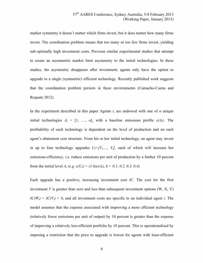
In the experiment described in this paper Agents i, are endowed with one of n unique

initial technologies Ai = [1, …, n], with a baseline emissions profile e(Ai). The

profitability of each technology is dependent on the level of production and on each

agent’s abatement cost structure. From his or her initial technology, an agent may invest

in up to four technology upgrades Ui=[Vi,…, Yi], each of which will increase her

emissions-efficiency, i.e. reduce emissions per unit of production by a further 10 percent

from the initial level Ai (e.g. e(Ui) = (1-k)e(Ai), k = 0.1, 0.2, 0.3, 0.4).

Each upgrade has a positive, increasing investment cost IC. The cost for the first

investment V is greater than zero and less than subsequent investment options (W, X, Y)

IC(Wi) > IC(Vi) > 0, and all investment costs are specific to an individual agent i. The

model assumes that the expense associated with improving a more efficient technology

(relatively fewer emissions per unit of output) by 10 percent is greater than the expense

of improving a relatively less-efficient portfolio by 10 percent. This is operationalised by

imposing a restriction that the price to upgrade is lowest for agents with least-efficient


9

initial technology and highest for agents with most efficient initial technology.

This model includes upgrade opportunities that maintain technology asymmetry through

the duration of the session. The added complexity allowed by the proportional upgrades

also allows for clearer application of this study’s findings. Since each agent type

maintains a unique value for a permit under this setup, the market provides a greater

opportunity to transact more efficiently.

In the experiment, some information about aggregate outcomes in individual periods is

provided to participants (the agents). Importantly, and in a departure from previous

studies (e.g. Camacho-Cuena & Requate, 2012) at the end of each period participants

were provided with information on the total number of upgrades (effectively units of

investment) that have been undertaken by all participants in that period. This design

choice was made to improve transparency in the lab (in the real world, firms are likely to

know once another firm has undertaken a large upgrade) and to minimize the magnitude

of the described coordination problem that has been found in previous studies (Requate

and Unold 2003; Camacho-Cuena and Requate 2012).

An aggregate desired emissions level E* is exogenously imposed by a regulator. The

regulator chooses either the emissions cap directly, or imposes a corresponding emissions

tax rate to ensure (at least in theory) that E* is attained. The aggregate emissions level E

is the sum of individual firms’ emissions, E = (ei)i=1

n

∑ . In this asymmetric market, the

theoretical setup was that some portion of the firms j (n – j, …, n) should upgrade their


10

technology, while the remaining firms (1, …, n-j-1) should not invest in abatement. A

regulator with full information can determine the minimum abatement costs and the

optimal upgrades for each agent according to the defined cap level or tax rate.

An agent with original technology i has an incentive to upgrade their technology until the

level at which the incremental upgrade costs (marginal abatement costs) equal the price

of emitting or the price of an input (either the tax rate or the equilibrium permit price). If

maximum profit with initial technology A is the production income less the cost C of

emitting with the initial technology at that level: π iAi = Yi −C(Ai) , and maximum profit

with upgraded technology production income less the cost C of emitting with the

upgraded technology less the investment costs IC: π iUi = Yi −C(Ui)− IC(Ui)

A

U

∑ , agent i

should upgrade until the investment costs equal the difference in the cost of emitting

IC(Ui)A

U

∑ = C(Ai)−C(Ui) .

In the model, agents know with full certainty the future tax level (when applicable), the

number of permits that they will be allocated once the cap is put into place (when

applicable), and the time at which the regulation with be implemented.

Under a tax, agents should invest until marginal investment costs equal the (known)

marginal tax rate. Under an ETS, future permit prices are unknown, so agents should wait

for information about other agents’ investments before executing their own investments.

Individuals’ optimal investment decisions depend on the emissions price (the tax, or a

permit’s traded price). In the theoretical parameters used in this study, the marginal tax


11

rate is within the range of equilibrium permit prices obtainable from an optimal aggregate

and individual investment behavior.

Theoretically, and as is the proclaimed policy objectives of cap and trade systems, agents

with the highest potential returns to investment relative to their investment costs (i.e.,

lower abatement costs) should move first and invest. Their early investment will provide

a signal to agents with higher abatement costs that there may be opportunities to purchase

permits at prices that are likely to be lower than their own abatement costs. Under perfect

information, the equilibrium level of investment and production theoretically converges

to the one under the tax regime. This design results with optimal investment levels that

are equivalent for each of the eight agents under all of the three regimes in a Nash

equilibrium. For each agent, the Nash equilibrium abatement investment and production

decisions are the same in all treatments.

4. Experimental Design and Procedure

We compare agents’ behavior under the three regulatory regimes (treatments) via an

economic experiment. The experiment was programmed and conducted with the software

z-Tree in an experimental laboratory at the University of Sydney (Fischbacher 2007).

Parameters and treatments

The participants’ (Agents’) task was to earn as much profit as possible during the

experimental session. Each Participant faced a unique linear production function, unique

investment costs and finite production capacity. Participants selected a production level


12

to maximize their income each period. They could invest in upgrades to increase their

efficiency. Participants played four rounds in a session. All rounds in a session were of

the same treatment, and participants maintained the same character endowments for the

four rounds.

A round consisted of 13 periods. Each period included three stages:

1. Investment Stage (60 seconds). At the start of every period (except for period

one), participants could invest in an upgrade that would reduce their emissions

(represented by their production costs) by 10 percent each. Emissions were

referred to as Inputs, and each production level required a certain number of

Inputs. An upgrade reduced the number of Inputs required per production level by

10 percent. Participants could select up to four incremental upgrades (one upgrade

per period). The maximum four upgrades would carry a cumulative 40 percent

reduction. Any upgrade was irreversible and lasted for all the remaining periods

in the round.

2. Production and Trading Stage (60 seconds). Participants selected a Production

Level between 0 and 10 each period. The costs (emissions) and profits associated

with each production level were known to participants. In the treatments with an

ETS, a single unit double auction was also active during this stage.

3. Summary Stage (15 seconds). Participants were shown a summary of their

personal performance for the previous period and the cumulative number of

investments undertaken by all participants in that period.


13

An experimental session consisted of 4 replications (rounds) of 13 periods. Participants

could earn income in each replication. Four replications per session were held in order to

allow for our observation of participants’ behavior before and after learning and to

control for noise. All rounds in a session were identical in that the same Treatment and

Producer characteristics were imposed for the duration of a round. Treatments were

characterized by the regulation type. Treatment 1 was a tax regime, Treatment 2 was a

hybrid regime, and Treatment 3 was an ETS regime. The first 5 periods of each round

were a liability-free phase, in which participants had the opportunity to produce with no

emissions costs, and to invest. The emissions regulation (tax or trading) was implemented

at period 6 of each round. Participants knew the sequence and timing of regime

implementation within a round in advance of the round’s beginning.

In the treatments with trading, emissions permits were symmetrically grandfathered to the

participants each period from the first period that trading became active. A single unit

double auction was selected as the trading mechanism in the designed environment due to

its easily understood and utilized design, particularly the ease of placing and accepting

bids and asks. Smith (1962) provides extensive evidence of the double auction’s tendency

to elicit best-possible market results in experimental environments. The findings

presented by Camacho-Cuena et al. (2012) strongly suggest that the type of auction used

after an initial distribution of permits does not have a significant effect on the pattern of

technology adoption in their environment which is similar to the one reported in the

present paper.


14

In periods with trading, the market for participants to buy and sell Inputs was open for 60

seconds.10 Participants could submit as many bids or asks (and buy and sell as many

Inputs) as they like within the trading period. Each bid or ask was for a single unit

(Input). The screen displayed the best current bid and ask at all times. To execute a trade,

buyers or sellers had to click on the bid or ask that they were willing to transact for. Each

transaction is for one Input. A record of each transacted price from the current period was

displayed on participants’ screens.11

Experimental Procedure

On entering the lab, each subject was randomly assigned a role as one of 8 Participants.

Each session was randomly assigned to one of the three treatments. Comprehensive

instructions about the game’s mechanism were provided in a video.12 After viewing,

participants completed a quiz to demonstrate their understanding of the instructions.

All participants were students at the University of Sydney who were recruited via the

University’s ORSEE database of student volunteers (Greiner 2004). Payments were in

Australian dollars. Each participant was given a A$10 show-up fee and could earn an

additional A$30 during the 2-hour session; participants took home an average of

A$33.21.13 Participants were informed of their personal exchange rate before beginning

10 Screenshots can be found in Appendix 2. 11 In advance of running the experiment sessions discussed in this paper, we ran a set of trial sessions. The purpose of these trials was to ensure that the software and instructions were robust. In advance of the trials, we considered setting a binding price floor for permits to be traded in the market. Because we observed trading prices in the paid trial were not extremely high or low (and we observed no price bubble or crash), we elected not to include a price floor in the experimental sessions described here. 12 Video instructions are available from the authors upon request. 13 This sum (A$20/hour) is slightly greater than a typical student job’s pay rate in Sydney.


15

the session. The exchange rates (Experimental dollars to Australian dollars) were

adjusted for each Participant’s characteristics so that each participant had the opportunity

to earn an equivalent payout (see exchange rates in Appendix 1). Each participant

participated in only one session.

5. Results

This section presents some preliminary results from the first set of sessions completed.

As of January 2013, three sessions per treatment were run (out of planned five). Each

session was comprised of four rounds. The behavior in the first round, fourth round and

overall is analyzed here to provide a cross-section of responses to the three regulations at

the initial experience, and after some learning has taken place. Behavior under the three

regulations was easily compared because each participant’s optimal behavior (Nash

Equilibria for investment magnitude and production level) is the same under each regime

(Figure 1).14

14 See Appendix Table 2 for a detailed list of optimal investment levels.


16

Figure 1 Optimal Investments

Investment cost efficiency

We measure investment cost efficiency as the actual costs incurred for efficiency

upgrades (investments) relative to the minimal (optimal) costs to be incurred under the

defined tax rate or a specified emissions cap: min IC(Ui)

i=1

n

∑

IC(Ui)i=1

n

∑.

We found that on average, participants overinvested most under the tax and least under

the ETS under the initial round of play (Figure 2).15

15 This result may be attributable to a tax aversion. The difference between treatments is not significant at a 90 percent significant level.


17

Figure 2 Investment Levels (Round 1)

Learning demonstrated in investment costs patterns

Overinvestment is found at different magnitudes in all treatments, but the extra costs

incurred by investing more heavily than necessary to achieve the defined cap are highest

in the initial round and decrease significantly (at a 99% confidence level) from Round 1

to Round 3 and 4 (Table 1).

Table 1 Comparison of total investment costs by Round (Bonferroni) ** p-value shows a difference between rounds at a 99% significance level

Round 1 2 3

2 -566.833 0.119

3 -1036.28 -469.444 p: 0.001*** 0.303

4 -1107.17 -540.333 -70.8889 p: 0.000*** 0.154 1.000

As seen in Figure 3, excess investment costs (meaning costs incurred by


18

overinvestments) clearly converge to zero (i.e., investment costs converge to the optimal)

under the tax and the ETS treatments (Figure 3). Excess investment costs do not follow

this trend under the hybrid treatment. Specifically, none of the hybrid observations

achieve as optimal investment patterns as do the two lowest ETS and tax sessions. Excess

costs decrease most in the tax treatment, second in the ETS and least in the hybrid. The

decrease in costs between Rounds 3 and 4 is not significant in any treatment, or overall.

The differences between treatments illustrated here are not significant at a 95%

confidence level. However, more sessions’ worth of data may yield greater insight in

terms of this measure.

Figure 3 Comparison of Extra Investment Costs incurred, by Round and Treatment

Differences in Investment, by Participant type

The parameters used in this experiment endow Participant 1 with the least efficient initial

technology (Ai) and Player 8 with the most efficient initial technology. Players 2 through


19

7 fall in a continuum from less to more efficient. In the first round, the participants with

the most extreme cost structures of initial technologies (highest and lowest efficiency)

consistently made significantly different investment decisions under the ETS than under

the tax or hybrid treatments. Specifically, Participant 8 underinvested under the ETS, and

overinvested under the tax and hybrid treatments. In the first round, the least efficient

participant (Player 1*), who should not have invested at all, overinvested in all treatments.

The magnitude of Player 1’s overinvestment was greater under the hybrid and ETS

treatments than tax (Figure 4).

Figure 4 Investment Level, by Participant type (Round 1)

Participants’ 1, 2 and 3, the low-efficiency participant types, are best off not upgrading

their technologies under Nash Equilibrium. In all treatments, these participants tended to

overinvest in early rounds, but invested closer to the zero (optimal) level in later rounds.

Later round investments patterns by low-efficiency players were closest to optimal (zero


20

investment) under the tax and furthest from optimal (most overinvestment) under the

ETS. Overall (and in Rounds 3 and 4), Players 1, 2 and 3 overinvest significantly more

under hybrid and ETS treatments than they do under the tax treatment (F = 8.06, p > F:

0.0006). Notably, even after upgrading, the efficiency of Players 1-3 was still so low that

their final opportunity cost of using a permit for production was lower than the price for

which they could sell it in the market.

The participants who start with moderately efficient technology (Participants 4 and 5)

underinvested overall and in the final rounds. Their investment levels did not

significantly differ across treatments.

The participants who start with the most efficient technologies (Participants 6, 7, 8)

overinvested overall and in the final rounds. Overinvestment levels were more equivalent

for the less-extreme participants (6 and 7) under the three treatments. This result

(underinvestment by less efficient participants and overinvestment by the more efficient)

is in line with the findings presented by Camacho-Cuena (2012) and Ganghadharan et al.

(2010). Participant 8 (very efficient) invested much closer to the optimal level under ETS

and tax than under hybrid in the fourth round (and underinvested under ETS overall)

(Figure 5).


21

Figure 5 Investment Level, by Participant type (Round 4)

Trading Efficiency

We define efficiency in trades as the difference in permits’ trading prices P to the

equilibrium price given the actual investment pattern, P*.

Trade Efficiency in a Period 11−mean(QP −QP*)

.

We observe lower trading prices for permits, higher trade efficiency, and lower volatility

in permits’ trading prices in the Hybrid treatment than ETS. Trade prices were

significantly less optimal (higher than the equilibrium) in the ETS than prices for permits

in the hybrid. Per the above definition, this means that trading efficiency is higher under

the hybrid regime than under the ETS. Overall, permits under the hybrid regime were

traded at prices significantly closer to the upper bound of the equilibrium price range than

were permit prices in the ETS treatments (p = 0.0391**).16 Trading prices observed under

16 We do not observe a significant difference in individual rounds, though this result may change with more observations.


22

the hybrid were significantly lower than ETS prices at a 95 percent significance level in

the initial two rounds. Higher volatility in trading prices during the initial period of first

round trading, and the overall volatility in the entirety of the first round of trading, was

greater in the ETS than the hybrid. We do not observe significant speculative trading in

either treatment.

Table 2 Summary of Mean Permit Prices and Standard Deviation by Round, Test for Equal Trade Efficiency

Hybrid R1 Hybrid R2 Hybrid R3 Hybrid R4

ETS R1

Hybrid: 19.61 (6.23) ETS: 23.90 (7.66)

F: 20.82 p: 0.0000***

ETS R2

Hybrid: 19.32 (7.35) ETS: 20.75 (3.95)

F: 4.65 p: 0.0319**

ETS R3

Hybrid: 17.79 (4.63) ETS: 20.18 (11.08)

F: 0.18 p: 0.6695

ETS R4

Hybrid: 19.98 (3.05) ETS: 19.74 (4.74) F: 0.33 p: 0.565

Overall Efficiency

We measure the overall efficiency of a market under a new regime as the minimum total

abatement cost divided by the actual total abatement cost

Profit with initial technology Ai

⇡

Ai

i = Yi � C(Ai) (1)

Profit with upgraded technology Ui = [V,W,X, Y ]

⇡

Ui

i = Yi � C(Ui)�UX

A

IC(Ui) (2)

Agents equate Investment Costs to di↵erence in production/abatement costs to maxi-mize profit:

UX

A

IC(Ui) = C(Ai)� C(Ui) (3)

Y : maximum production incomeC(xi) = P(number of permits bought in the market) + F(number of permits not held)

if P: trade price for permits in the market, and F: tax or fee per permit worthof emissionThis can be negative if an agent’s profit in the permit market exceeds the feesincurred.

aggregate emissions

E =nX

i=1

(ei) (4)

investment e�ciencymin.

Pni=1 IC(Ui)Pn

i=1 IC(Ui)(5)

Trade E�ciency1

1�mean(QP �QP

⇤)(6)

Overall E�ciencyTAC

⇤

TAC

(7)

min.

Pni=1 IC

⇤(U⇤i ) + (Y ⇤

0 � Y

⇤R)Pn

i=1 IC(Ui) + (Y0 � YR)(8)

TAC

min

nX

i=1

IC(Ui) + (Y0 � YR) (9)

1

. Total abatement costs

(TAC) are made up of aggregate investment costs (IC), reduction in production income at

the profit-maximizing production levels from a restriction-free period (0) to the regulated

period (R) and taxes due. The optimal total abatement cost, TAC*, can be denoted:


23

IC(Ui)+(Y 0 −YR)i=1

n

∑ + Tax, and overall efficiency:

Overall Efficiency: min IC*(Ui

*)+(Y0 −YR*)+Tax*

i=1

n

∑IC(Ui )+(Y0 −YR )+Tax

i=1

n

∑

Overall efficiency is highest in the tax treatment and lowest in the ETS treatment. We

observe a significant difference between the overall efficiency in the tax versus ETS

treatments in all periods (p=0.0537*) and in the last two rounds (p = 0.0317**).

6. Discussion and Conclusion

The objective of this study was to investigate and compare efficiencies under different

regulations via experimental methods. Strategic uncertainty under a new cap and trade

(ETS) is known to motivate suboptimal investment patterns (both over and under-

investment) among liable firms, and potentially inefficient and volatile trading in a permit

market. We developed an economic experiment to test whether there would be a

difference in the behavioural responses to three different regimes, with all characteristics

of the environment held constant except for the nature of the regulation.

It has been suggested that a temporary tax, in place for some time in advance of the ETS

system, might reduce strategic uncertainty enough to elicit significantly more optimal

investment patterns. In this study, we were interested in exploring whether use of a tax as

an introduction to a cap and trade regime would motivate more efficient investments and

behavior in the permit market than would a simple cap and trade (ETS) regime during the


24

implementation period.

Specifically, we hypothesized that the higher certainty characteristic of a tax would yield

more efficient decisions under a full tax than the other two regimes, and that

implementing a temporary tax in advance of a trading system would result in higher

efficiency under a hybridized regulation than an ETS regime.

Preliminary results suggest that both the hybrid and ETS systems have relative strengths

and weaknesses in the laboratory environment. These results show that as expected,

participants invest more efficiently under a tax regime than under an ETS regime.

However, early tests of the results do not show a significant difference between

investment efficiency under the hybrid system to ETS. Contrary to our hypotheses, we

observe that participants overinvest at a slightly higher magnitude under the hybrid

system than under a simple ETS regime. We hypothesize that the relatively suboptimal

decisions may result from the added complexity of the regulating rules.

The hybridized system does not always perform worse than the ETS. Specifically, use of

a tax as introduction to an ETS seems to result in more efficient permit market behavior

than does a simple ETS (permits are traded at prices that are lower and closer to the upper

bound equilibrium price level in the hybrid treatments than the ETS). These results

indicate that a greater certainty with regards to return on investments in abatement

ultimately informs a more efficient market. This result warrants further study, with

particular attention to be paid to how much the tax rate acts as a strong price anchor. In

the current parameters, the tax rate equals the equilibrium price under a perfect


25

investment pattern, and there is no price ceiling. A reasonable next step would be to

investigate how behavior would react under a suboptimal (too high or too low) short-term

tax rate, or within a market with a price floor or price ceiling.

We plan to next explore the effect of an additional layer of political uncertainty on these

behaviours. We are in the process of developing additional treatments that will allow us

to further investigate whether less certainty about future regulations results in a

significantly less-efficient market than do the full-certainty treatments. Specifically, we

plan to introduce uncertainty about the implementation, or timing of an implementation

of a planned future ETS, and then study the effect of this additional uncertainty on

investment and market efficiency.

It should not be overlooked that due to the limited number of observations, the results

presented in this version of the paper are preliminary. We plan to gather additional

observations from the same setup and treatments that we have presented here in order to

test the treatments more thoroughly.


26

References Aldy, J. and R. Stavins (2011). The promise and problems of pricing carbon: theory

and experience. Faculty Working Paper Series, Harvard Kennedy School. Aldy, J. and R. Stavins (2012). "The Promise and Problems of Pricing Carbon: Theory

and Experience." The Journal of Environment & Development 21(2): 152-‐180.

Betz, R. and A. Gunnthorsdottir (2009). Modeling emissions markets experimentally: The impact of price uncertainty. 18th World IMACS / MODSIM Congress. Cairns.

Bohm, P. (2003). Experimental evaluations of policy instruments. Handbook of Environmental Economics. K. G. Mäler and J. R. Vincent. 1: 437-‐460.

Camacho-‐Cuena, E. and T. Requate (2012). "Investment Incentives Under Emission Trading: An Experimental Study." Environmental and Resource Economics 53(2): 229.

Downing, P. and L. White (1986). "Innovation in Pollution Control." Journal of Environmental Economics and Management 13: 18-‐29.

Drape, J. (2012). Carbon tax debate will rage on: Combet. Sydney Morning Herald. Sydney, Fairfax Media.

Fischbacher, U. (2007). "z-‐Tree: Zurich Toolbox for Ready-‐made Economic Experiments." Experimental Economics 10(2): 171-‐178.

Gangadharan, L. (2005). Investment Decisions and Emissions Reductions: Results from Experiments in Emissions Trading. Department of Economics Research Paper. U. o. Melbourne. 42.

Greiner, B. (2004). An Online Recruitment System for Economic Experiments. Forschung und wissenschaftliches Rechnen 2003. V. M. E. Kurt Kremer. Göttingen : Ges. für Wiss. Datenverarbeitung. 79-‐93.

Hahn, R. W. and R. N. Stavins (2011). "The Effect of Allowance Allocations on Cap-‐and-‐Trade System Performance." Journal of Law and Economics 54(November 2011): S267-‐296.

Kahneman, D. and A. Tversky (1979). "Prospect Theory: An Analysis of Decision under Risk." Econometrica 47(2): 263-‐292.

Kelly, P. (2009). Renewable energy target initiative is mad, bad tokenism. The Australian.

Kneese, A. V. and C. L. Schultze (1975). Pollution, prices, and public policy. Washington, DC, Resources for the Future, Inc. and the Brookings Institution.

Malueg, D. (1989). "Emission Credit Trading and the Incentive to Adopt New Pollution Abatement Technology’." Journal of Environmental Economics and Management 16: 52-‐57.

Pezzey, J. and F. Jotzo (2012). "Tax-‐versus-‐trading and efficient revenue recycling as issues for greenhouse gas abatement." Journal of Environmental Economics and Management 64(2): 230-‐236.

Requate, T. (2005). "Dynamic incentives by environmental policy instruments—a survey." Ecological Economics 54(2–3): 175-‐195.


27

Requate, T. and W. Unold (2003). "Environmental policy incentives to adopt advanced abatement technology: Will the true ranking please stand up?" European Economic Review 47(1): 125-‐146.

Shanahan, D. (2012). Opposition leader will not be for turning on 'toxic' carbon tax. The Australian.

Smith, V. (1962). "An Experimental Study of Competitive Market Behavior." The Journal of Political Economy 70(2): 111-‐137.

Tietenberg, T. (2006). Emissions Trading: Principles And Practice. Washington, DC.

Appendices

Appendix 1: Tables

Appendix Table 1: Exchange Rates (E$ to AU$1)

Treatment 1 (Tax)

Treatment 2 (Hybrid)

Treatment 3 (Cap and Trade) Subject

1 E$50 E$103 E$135 2 67 120 152 3 83 137 169 4 111 164 195 5 154 207 239 6 190 243 275 7 226 280 312 8 263 316 348

Appendix Table 2: Optimal Investment Level and Cost, by Participant Type

Participant 1 2 3 4 5 6 7 8 Total Optimal Upgrade

Level 0 0 0 3 3 2 1 1 10

Optimal Investment Cost (E$)

0 0 0 225 225 150 75 125 800


28

Appendix Table 3: Average Number of Upgrades above Optima

Round

Treatment 1 2 3 4 Totals by Treatment

Tax 48 24 14 12 78 Hybrid 44 33 26 26 129

ETS 45 34 28 26 133

Appendix Table 4: Average Overall Efficiency by Round and Treatment

Round

Treatment 1 2 3 4 Overall

Average by Treatment

Tax .593 .785 .812 .825 .754 Hybrid .535 .607 .721 .763 .657

ETS .534 .610 .683 .731 .640


29

Appendix 2: Selected zTree screenshots

Participants’ Screen, Investment Stage

Participants’ Screen, Production Stage, with Trading


30

(Bohm 2003)

(Pezzey and Jotzo 2012)

(Smith 1962)

(Fischbacher 2007)

(Gangadharan 2005)

Abatement Investment Decisions under Alternative Emissions ...

Documents

Transcript of Abatement Investment Decisions under Alternative Emissions ...