Electricity Consumption and Asset Prices · Electricity Consumption and Asset Prices Abstract ......
52
0 Electricity Consumption and Asset Prices Zhi Da and Hayong Yun * First draft: April 2010 This draft: September 2010 * Authors’ addresses: Zhi Da is at the Department of Finance, 239 Mendoza College of Business, University of Notre Dame, Notre Dame, IN 46556. Tel. (574) 631-0354, E-mail: [email protected]. Hayong Yun is at the Department of Finance, 242 Mendoza College of Business, University of Notre Dame, Notre Dame, IN 46556. Tel. (574) 631- 9322, Fax. (574) 631-5255, E-mail: [email protected]. We thank Tom Cosimano, Ravi Jagannathan, Bill McDonald, Starvos Panageas, Jesper Rangvid, Marco Rossi, Alexi Savov, Tom Smith, Raman Uppal, Annette Vissing- Jorgensen, Xiaoyan Zhang and seminar participants at Australian National University, the Asset Pricing Workshop at ESSFM (Gerzensee), and the State of Indiana Conference (Indiana University, Purdue University and University of Notre Dame) for helpful comments. We thank Manisha Goswami, Steve Hayes, Dongyoup Lee, Hang Li, Liang Tan, Yan Xu and Wei Yang for data and programming support. We thank Wayne Ferson, Amit Goyal, Ken French, Martin Lettau, and Alexi Savov for making their data available.
Transcript of Electricity Consumption and Asset Prices · Electricity Consumption and Asset Prices Abstract ......

0
Electricity Consumption and Asset Prices
Zhi Da and Hayong Yun*
First draft: April 2010 This draft: September 2010
* Authors’ addresses: Zhi Da is at the Department of Finance, 239 Mendoza College of Business, University of Notre Dame, Notre Dame, IN 46556. Tel. (574) 631-0354, E-mail: [email protected]. Hayong Yun is at the Department of Finance, 242 Mendoza College of Business, University of Notre Dame, Notre Dame, IN 46556. Tel. (574) 631-9322, Fax. (574) 631-5255, E-mail: [email protected]. We thank Tom Cosimano, Ravi Jagannathan, Bill McDonald, Starvos Panageas, Jesper Rangvid, Marco Rossi, Alexi Savov, Tom Smith, Raman Uppal, Annette Vissing-Jorgensen, Xiaoyan Zhang and seminar participants at Australian National University, the Asset Pricing Workshop at ESSFM (Gerzensee), and the State of Indiana Conference (Indiana University, Purdue University and University of Notre Dame) for helpful comments. We thank Manisha Goswami, Steve Hayes, Dongyoup Lee, Hang Li, Liang Tan, Yan Xu and Wei Yang for data and programming support. We thank Wayne Ferson, Amit Goyal, Ken French, Martin Lettau, and Alexi Savov for making their data available.

1
Electricity Consumption and Asset Prices
Abstract
Electricity consumption is a good real-time proxy for economic activities as most modern-day
economic activities involve the use of electricity, which cannot be easily stored. Empirically, electricity
consumption data is widely available in high frequency at both aggregate and disaggregate level, allowing
several exciting asset pricing applications. First, we demonstrate that electricity usage is a better measure
of spot consumption as in the CCAPM and that an electricity-based CCAPM does well in both time-series
and cross-sectional asset pricing tests. In the U.S., December-to-December total electricity consumption
growth matches the equity premium with a relative risk aversion of 17.3 and a more reasonable implied
risk-free rate than those obtained from the standard NIPA consumption measures. This result is not driven
by the electricity consumption due to production activities and extreme weather fluctuations. Second, we
confirm the calendar effect in consumption documented in Jagannathan and Wang (2007) using monthly
electricity data and test the model of Constantinides and Duffie (1996) based on incomplete market and
uninsurable income shocks using state-level electricity data. Finally, we find that industrial usage of
electricity, capturing business cycle variation in real time, does a good job in predicting future stock
excess returns at both market and industry level.
Keywords: Consumption-based Capital Asset Pricing Model (CCAPM), electricity consumption, Return
Predictability.

2
1. Introduction
A fundamental question in financial economics is how economic activities such as consumption
and production and the related business cycle fluctuation affect asset prices. While a long strand of
literature has made successful attempts in addressing this question from a theoretical prospective,
empirical attempts in linking economic activities to asset pricing had limited success. For example, it is
well known that the growth rate in the standard NIPA consumption measure (real per capita personal
expenditure on nondurable goods and services) is too smooth to justify the observed equity risk premium
in U.S. (Mehra and Prescott (1985)). In addition, traditional macroeconomic variables have proven
especially dismal in predicting future stock returns (Lettau and Ludvigson (2001)). In this paper, we
examine electricity usage as a new real-time proxy of economic activities. We find that electricity usage
does a good job in explaining stock returns in both time-series and cross-section within the consumption-
based asset pricing framework. It also does a good job in capturing business cycle fluctuations and
predicts future stock excess returns.
In modern life, most economic activities involve the use of electricity. For example, when
preparing a meal, food may have been stored in a freezer, defrosted in a microwave oven, cooked in an
electric oven, and eaten while watching a sports game aired on TV. Shopping malls may use an extra
amount of electricity during the winter holiday season to be open longer hours and to power ornamental
lights. We, therefore, expect residential and commercial usage of electricity to be a good proxy for
consumption. In addition, factories typically use electricity in production, suggesting industrial usage of
electricity to be a good proxy for economic output and the business cycle fluctuation. For example,
Comin and Gertler (2006) use electricity usage to measure production activity in their study of business
cycle. Due to technological limitations, electricity cannot be easily stored: once produced, it has to be
either consumed or wasted. As a result, electricity usage more likely tracks economic activities in real
time.
Since electric utilities are highly regulated and are subject to extensive disclosure requirements,
electricity usage data are accurately measured at high frequency and are available at a disaggregated level.

3
For example, in the United States, monthly electricity consumption information is available from 1960 to
the present, by state and by user types. In the United Kingdom, electricity consumption information is
available by half-hours since 2001, and daily since 1970. In the EU, monthly electricity consumption is
available from 1990 to the present. Annual electricity consumption is available for many other countries
in the world. Taking advantage of the availability of electricity consumption data, we examine several
asset pricing applications empirically.
In the first application, we examine electricity usage as a proxy for aggregate consumption in the
context of the standard Consumption-based Capital Asset Pricing Model (CCAPM) of Lucas (1978) and
Breeden (1979). In an effort to reconcile the observed high equity premium and low consumption risk
within the CCAPM framework, extant literature has explored modifications in investor preferences,
implications of incomplete markets, market imperfections and alternative ways of measuring aggregate
consumption risk.1 Recently, Savov (2010) proposed an alternative approach using annual garbage
generation as a measure of consumption, which is twice as volatile as the standard NIPA consumption
measure (real per capita personal expenditure on nondurable goods and services) and highly correlated
with market returns. As a result, this measure yields a more modest implied relative risk aversion
coefficient than those obtained using conventional NIPA consumption expenditures. We complement
Savov (2010) by showing that a simple and novel measure of consumption goes a long way in
resurrecting the standard CCAPM.
Compared to existing consumption measures including garbage generation, electricity
consumption has at least two advantages which make it potentially a better candidate for testing the
standard CCAPM.
First, we expect electricity consumption to likely reflect investors’ consumption activities in a
real time manner. In contrast, the popular NIPA consumption data is smoothed with the X-11 seasonal
1 Related papers include Sundaresan (1989), Constantinides (1990), Epstein and Zin (1991), Campbell and Cochrane (1999), Bansal and Yaron (2004), Hansen, Heaton, and Li (2008), Malloy, Moskowitz, and Vissing-Jorgensen (2009)), Constantinides and Duffie (1996), Mankiw and Zeldes (1991), Constantinides, Donaldson, and Mehra (2002), Ait-Sahalia, Parker, and Yogo (2004), Parker and Julliard (2005), Jagannathan and Wang (2007), and Jagannathan, Takehara, and Wang (2007)).
4
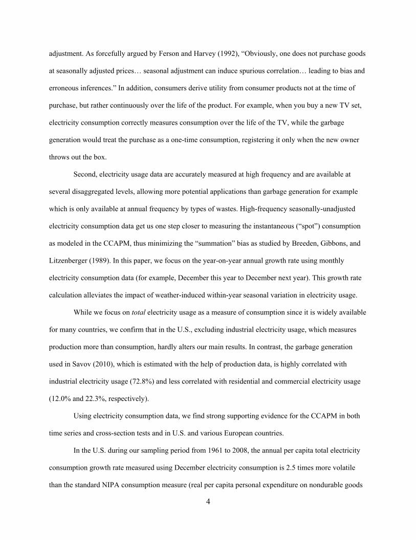
adjustment. As forcefully argued by Ferson and Harvey (1992), “Obviously, one does not purchase goods
at seasonally adjusted prices… seasonal adjustment can induce spurious correlation… leading to bias and
erroneous inferences.” In addition, consumers derive utility from consumer products not at the time of
purchase, but rather continuously over the life of the product. For example, when you buy a new TV set,
electricity consumption correctly measures consumption over the life of the TV, while the garbage
generation would treat the purchase as a one-time consumption, registering it only when the new owner
throws out the box.
Second, electricity usage data are accurately measured at high frequency and are available at
several disaggregated levels, allowing more potential applications than garbage generation for example
which is only available at annual frequency by types of wastes. High-frequency seasonally-unadjusted
electricity consumption data get us one step closer to measuring the instantaneous (“spot”) consumption
as modeled in the CCAPM, thus minimizing the “summation” bias as studied by Breeden, Gibbons, and
Litzenberger (1989). In this paper, we focus on the year-on-year annual growth rate using monthly
electricity consumption data (for example, December this year to December next year). This growth rate
calculation alleviates the impact of weather-induced within-year seasonal variation in electricity usage.
While we focus on total electricity usage as a measure of consumption since it is widely available
for many countries, we confirm that in the U.S., excluding industrial electricity usage, which measures
production more than consumption, hardly alters our main results. In contrast, the garbage generation
used in Savov (2010), which is estimated with the help of production data, is highly correlated with
industrial electricity usage (72.8%) and less correlated with residential and commercial electricity usage
(12.0% and 22.3%, respectively).
Using electricity consumption data, we find strong supporting evidence for the CCAPM in both
time series and cross-section tests and in U.S. and various European countries.
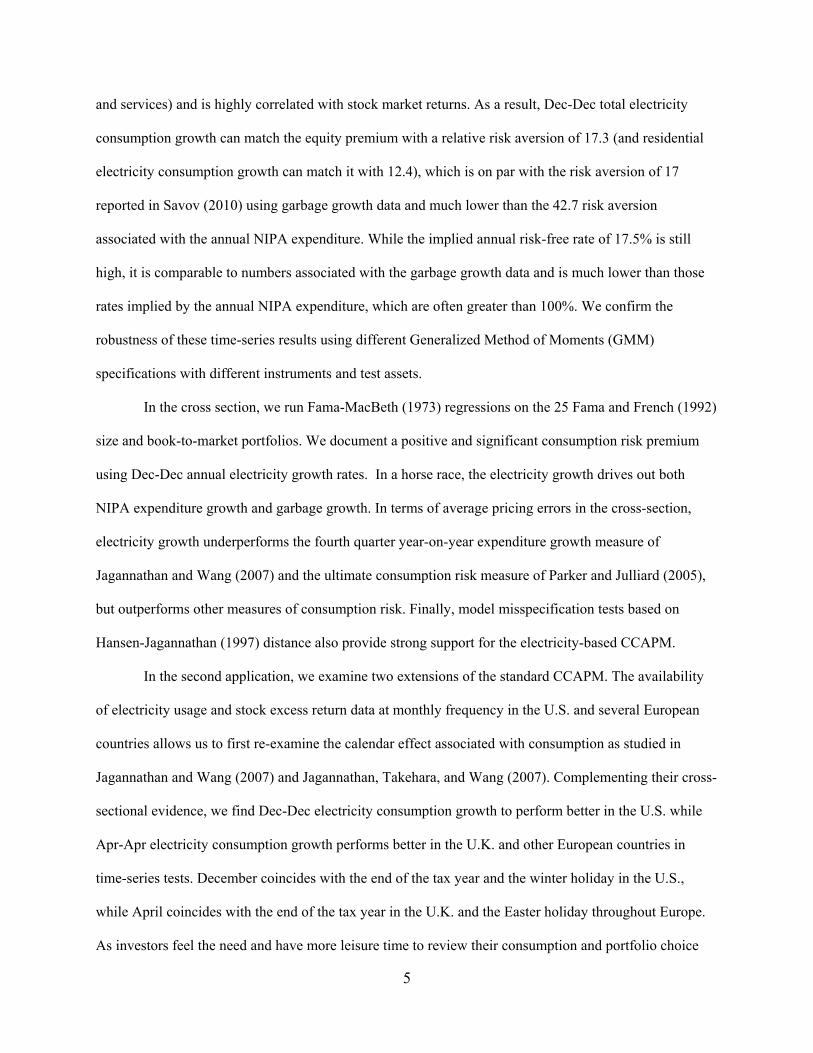
In the U.S. during our sampling period from 1961 to 2008, the annual per capita total electricity
consumption growth rate measured using December electricity consumption is 2.5 times more volatile
than the standard NIPA consumption measure (real per capita personal expenditure on nondurable goods
5
and services) and is highly correlated with stock market returns. As a result, Dec-Dec total electricity
consumption growth can match the equity premium with a relative risk aversion of 17.3 (and residential
electricity consumption growth can match it with 12.4), which is on par with the risk aversion of 17
reported in Savov (2010) using garbage growth data and much lower than the 42.7 risk aversion
associated with the annual NIPA expenditure. While the implied annual risk-free rate of 17.5% is still
high, it is comparable to numbers associated with the garbage growth data and is much lower than those
rates implied by the annual NIPA expenditure, which are often greater than 100%. We confirm the
robustness of these time-series results using different Generalized Method of Moments (GMM)
specifications with different instruments and test assets.
In the cross section, we run Fama-MacBeth (1973) regressions on the 25 Fama and French (1992)
size and book-to-market portfolios. We document a positive and significant consumption risk premium
using Dec-Dec annual electricity growth rates. In a horse race, the electricity growth drives out both
NIPA expenditure growth and garbage growth. In terms of average pricing errors in the cross-section,
electricity growth underperforms the fourth quarter year-on-year expenditure growth measure of
Jagannathan and Wang (2007) and the ultimate consumption risk measure of Parker and Julliard (2005),
but outperforms other measures of consumption risk. Finally, model misspecification tests based on
Hansen-Jagannathan (1997) distance also provide strong support for the electricity-based CCAPM.
In the second application, we examine two extensions of the standard CCAPM. The availability
of electricity usage and stock excess return data at monthly frequency in the U.S. and several European
countries allows us to first re-examine the calendar effect associated with consumption as studied in
Jagannathan and Wang (2007) and Jagannathan, Takehara, and Wang (2007). Complementing their cross-
sectional evidence, we find Dec-Dec electricity consumption growth to perform better in the U.S. while
Apr-Apr electricity consumption growth performs better in the U.K. and other European countries in
time-series tests. December coincides with the end of the tax year and the winter holiday in the U.S.,
while April coincides with the end of the tax year in the U.K. and the Easter holiday throughout Europe.
As investors feel the need and have more leisure time to review their consumption and portfolio choice

6
decisions during these times, the CCAPM should perform better. Our findings thus support the optimal
inattention to the stock market in Abel, Eberly, and Panageas (2007).
Taking advantage of the availability of state-level annual electricity usage data in the U.S., we
test the model of Constantinides and Duffie (1996) based on uninsurable income shocks. We consider
electricity usage in a state as a proxy for the consumption of a synthetic cohort in that state. Within this
framework, we can match the equity premium with a relative risk aversion of about 18 during the period
1961-2008. The required risk aversion parameter is similar to that found by Jacobs, Pallage, and Robe
(2005) who use alternative state-level consumption data based on retail sales. The results confirm that
electricity usage is indeed a good measure of consumption at both the aggregate and the state level. In
addition, the fact that aggregate U.S. electricity consumption and state-level electricity consumption yield
similar required risk aversion parameters suggests that the incomplete market assumption might not be
necessary when aggregate consumption is better measured. Finally, by linking state-level electricity
growth to state-level weather fluctuation, we also confirm that weather change is unlikely driving the
main results in our paper.
In the third application, we examine the performance of electricity growth rate in predicting
future stock excess returns. The question of return predictability is central for asset pricing, portfolio
choice, and risk management. The general finding in the literature is that only financial indicators not
macroeconomic business cycle indicators predict stock returns (see Campbell (2003), Cochrane (2007)
and Lettau and Ludvigson (2009) among others). This finding is discomforting as expected returns should
ultimately be linked to movements in economic output, consumption and the business cycle.
We show that December-to-December industrial electricity growth, which is a purely quantity-
based macroeconomic indictor, captures business cycle variations well. Its correlation with an annual
NBER recession variable is 57%. While electricity usage data is observed with minimum delay, the
NBER recession dates are often announced with significant lag, so industrial electricity growth captures
business cycle on a timelier basis. As a result, in our sampling period from 1961 to 2003, the industrial
electricity growth does a good job in predicting future stock excess returns at both market and industry

7
level.2 The in-sample R2 is 9.7% when predicting next-year market excess return and is about 20% when
predicting the next-year industry excess returns for several industries (such as nondurables and shops).
When compared to a comprehensive list of predictive variables studied in Goyal and Welch (2008), our
industrial electricity growth variable only underperforms the cay variable of Lettau and Ludvigson (2001)
and the equity issuance variable (eqis) in terms of in-sample R2. The predictive coefficient on our
industrial electricity growth variable is negative and significant, consistent with a counter-cyclical market
risk premium, as predicted by theoretical models such as Campbell and Cochrane (1999). Furthermore,
the cross-industry variation in predictive power is consistent with the differential industry systematic risk
exposures proxied using the Fama-French (1993) three-factor loadings.
The rest of the paper proceeds as follows. Section 2 describes the datasets used for this study and
provides summary statistics of the main variables. Section 3 presents evidence supporting the standard
CCAPM from the U.S. in time-series as well as in cross-sectional tests. Section 4 examines the calendar
cycle effect in consumption in both U.S. and European countries and tests an incomplete market model
using state-level electricity consumption data. Section 5 applies electricity data in return predictability
tests. Section 6 provides concluding remarks.
2. Data
2.1. Data construction
This paper uses two main sets of data: various measures of consumption and stock return data.
The monthly U.S. electricity consumption data are manually collected from two sources: Electric Power
Statistics for 1960–1978 and from Electric Power Monthly for 1979–2009. These documents are
published each month by the Energy Information Administration (EIA), and report sales of electric
energy (in millions of kilowatthours) to ultimate customers for residential customers, commercial
2 We end our sampling period at 2003 because of a change in the definition of user type in 2003 which makes industry electricity growth rate less comparable before and after 2002. If we ignore this “structure break” and extend our sampling period to 2008, we obtain very similar results. In fact, the relative performance of industrial electricity growth rate actually improves.

8
customers, industrial customers, other customers, and the U.S. total in each month.3 As electricity
consumption data could be revised later by the EIA, our hand collection of vintage data minimizes any
potential forward-looking bias, which is an important concern when conducting return predictability tests.
We also collect information on state-level (annual) electricity consumption from the EIA State Energy
Data System during 1960 to 2009. Corresponding annual state population data is obtained from
Surveillance Epidemiology and End Results (SEER) and U.S. Census Bureau population estimates.
In order to compare results from electricity consumption growth with those from other
consumption measures, we use real per capita expenditure data from the National Income and Product
Accounts (NIPA) of the Bureau of Economic Analysis. We add seasonally adjusted personal consumption
expenditures of services and nondurable goods for 1960–2008. In addition, we obtain quarterly
seasonally-unadjusted personal expenditure data for services and nondurable goods from Wayne Ferson’s
website. According to a study by Ferson and Harvey (1992), the seasonally-unadjusted personal
consumption expenditure data is considered to be a more accurate measure in terms of the timing of
consumption. Annual garbage data from the U.S. Environmental Protection Agency (EPA) from 1960 to
2008 are kindly provided to us by Alexi Savov. As in Savov (2010), we exclude yard trimmings from the
total garbage generation.
We match these consumption data with U.S. stock returns and one-month Treasury bill returns,
which we obtain from CRSP tape provided by Wharton Research Data Services for the 1960-2008 period.
We match this data with the Fama and French 25 portfolios based on size and book-to-market, which are
obtained from Kenneth French’s website. We also obtain the consumption-wealth ratio (“cay”) from
Martin Lettau’s website (Lettau and Ludvigson (2001)). Following Campbell (1999) and Savov (2010),
3 Based on the description of EIA Form 826, the residential sector consists of living quarters for private households. The commercial sector consists of service-providing facilities such as businesses, governments, and institutional living quarters. The industrial sector consists of facilities for producing goods, such as manufacturing (NAICS codes 31-33); agriculture, forestry, and hunting (NAICS code 11); mining, including oil and gas extraction (NAICS code 21); natural gas distribution (NAICS code 2212); and construction (NAICS code 23). Other customers include public street and highway lighting, public authorities, railroads and railways, and irrigation, as well as interdepartmental sales. Total electricity consumption accounts for the amount used by ultimate customers, and hence excludes resold or wasted amounts. It also excludes direct use, which is self-used, e.g., electricity used in power plants for generating electricity.

9
we use the beginning-of-period time convention when matching return data to all year-on-year growth
rates computed using annual data. For instance, the calendar year return in year t will be matched to the
garbage growth computed using annual garbage generation in year t and t+1. For this reason, most of our
time series tests stop at year 2008 and those involving garbage growth stop at year 2007.
The electricity consumption data for the European Union are provided by the European Network
of Transmission System Operators for Electricity (ENTSO-E). Excluding the U.K., there are 10 countries
that have reported their monthly electricity consumption through ENTSO-E since 1990. Among these
countries, we include the eight for which we were able to find matching monthly stock return and risk-
free rate data: Belgium, France, Germany, Italy, Netherlands, Portugal, Spain, and Switzerland. These
monthly electricity consumption data are then merged with each country’s stock market return and risk-
free rate data from Datastream. In the U.K., electricity consumption is more extensively reported than in
other EU countries. The National Grid of the United Kingdom records daily electricity consumption data
from 1971 to 2005, and half-hourly electricity consumption data from April 2001 to the present. To be
consistent with the rest of the electricity data, we aggregate daily and half-hourly electricity consumption
data at the monthly level from 1971 to 2008. This monthly U.K. electricity consumption data is merged
with monthly U.K. stock market returns from Datastream in the same sampling period.
Finally, in our return predictability tests, we consider a comprehensive list of predictive variables
studied in Goyal and Welch (2008). These variables at annual frequency are downloaded from Amit
Goyal’s website.
Using these consumption and stock market return data, we construct year-on-year consumption
growth and market returns for each month. There are three main reasons for focusing on year-on-year
monthly electricity consumption growth. First, the standard CCAPM requires seasonally-unadjusted spot
consumption growth, which is best proxied by year-on-year monthly electricity growth (Breeden,
Gibbons, and Litzenberger (1989)). Second, as in Jagannathan and Wang (2007), this focus allows us to
examine the calendar effects of the CCAPM, where various discretionary consumption decisions are
clustered within each month (e.g., holiday shopping, fiscal year-end tax decisions, realization of annual

10
bonuses). Finally, electricity consumption data are exposed to strong within-year seasonal effects, such as
weather fluctuations.
Figure 1 shows the normalized electricity demand for each month (Panel A) and the deviation of
energy degree days in each month from its historical mean divided by its historical standard deviation
(Panel B). As shown in the figure, average monthly variations in weather conditions and electricity
demands within a year are positively correlated. This positive correlation is stronger for residential and
commercial electricity usage.4 Year-on-year electricity consumption growth identifies changes in
consumption due to changes in economic conditions rather than seasonal weather effects. One may argue
that year-on-year electricity consumption growth is still subject to residual weather effects (for instance,
February 2010 is unusually cold). Such extreme weather conditions are less likely to occur during months
in the second and fourth quarters, such as April and December, which partly explains why Apr-Apr and
Dec-Dec electricity consumption works better in Europe and in the U.S. respectively. In addition, we
work to eliminate extreme weather variations from year-on-year electricity consumption growth and focus
on what remains. Unreported results suggest that residual electricity consumption growth (orthogonal to
weather change) performs similarly in various CCAPM tests. In section 4.2, we further confirm that
repeating our tests in different states with different weather exposure generates very similar results. These
results are intuitive: since stock market returns are unlikely to be driven by weather changes, the success
of electricity growth in explaining stock market data is unlikely to be attributable to weather change.
2.2. Summary statistics
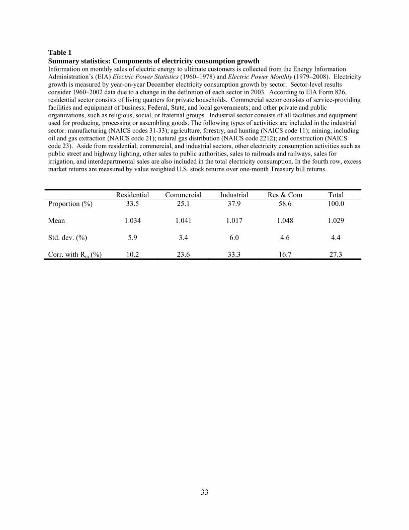
Table 1 shows the summary statistics for each component of electricity consumption. Per capita
electricity consumption growth rates are measured year-on-year in December. As shown in the first row,
three major components (residential, commercial, and industrial customers) are evenly represented in the
4 According to the 2007 10-K filing of Empire District Electric Co., “very hot summers and very cold winters increase electric demand, while mild weather reduces demand. Residential and commercial sales are impacted more by weather than industrial sales, which are mostly affected by business needs for electricity and by general economic conditions.”
11
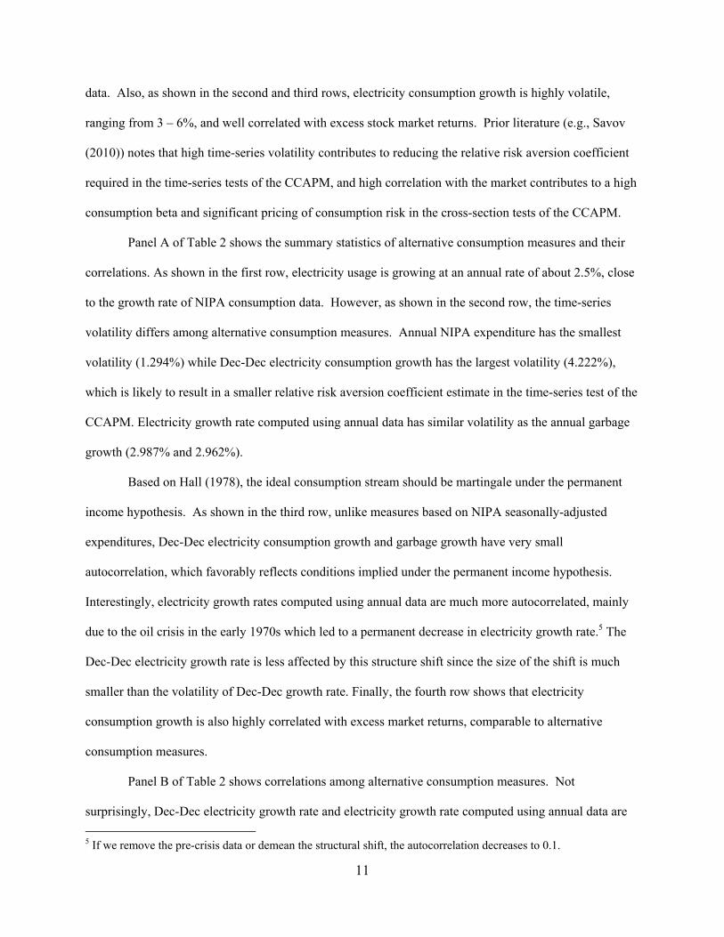
data. Also, as shown in the second and third rows, electricity consumption growth is highly volatile,
ranging from 3 – 6%, and well correlated with excess stock market returns. Prior literature (e.g., Savov
(2010)) notes that high time-series volatility contributes to reducing the relative risk aversion coefficient
required in the time-series tests of the CCAPM, and high correlation with the market contributes to a high
consumption beta and significant pricing of consumption risk in the cross-section tests of the CCAPM.
Panel A of Table 2 shows the summary statistics of alternative consumption measures and their
correlations. As shown in the first row, electricity usage is growing at an annual rate of about 2.5%, close
to the growth rate of NIPA consumption data. However, as shown in the second row, the time-series
volatility differs among alternative consumption measures. Annual NIPA expenditure has the smallest
volatility (1.294%) while Dec-Dec electricity consumption growth has the largest volatility (4.222%),
which is likely to result in a smaller relative risk aversion coefficient estimate in the time-series test of the
CCAPM. Electricity growth rate computed using annual data has similar volatility as the annual garbage
growth (2.987% and 2.962%).
Based on Hall (1978), the ideal consumption stream should be martingale under the permanent
income hypothesis. As shown in the third row, unlike measures based on NIPA seasonally-adjusted
expenditures, Dec-Dec electricity consumption growth and garbage growth have very small
autocorrelation, which favorably reflects conditions implied under the permanent income hypothesis.
Interestingly, electricity growth rates computed using annual data are much more autocorrelated, mainly
due to the oil crisis in the early 1970s which led to a permanent decrease in electricity growth rate.5 The
Dec-Dec electricity growth rate is less affected by this structure shift since the size of the shift is much
smaller than the volatility of Dec-Dec growth rate. Finally, the fourth row shows that electricity
consumption growth is also highly correlated with excess market returns, comparable to alternative
consumption measures.
Panel B of Table 2 shows correlations among alternative consumption measures. Not
surprisingly, Dec-Dec electricity growth rate and electricity growth rate computed using annual data are 5 If we remove the pre-crisis data or demean the structural shift, the autocorrelation decreases to 0.1.

12
highly correlated (50.6%). In addition, Dec-Dec electricity consumption growth is also highly correlated
with annual garbage growth (33.3%), annual personal consumption expenditure (35.4%) and with the Q4-
Q4 measure (55.9%). Finally, when growth rates are all computed using annual data, expenditure growth
is more correlated with electricity growth (67.5%) than with garbage growth (52.8%). These results are
also confirmed in Figure 2, which shows that electricity consumption growth has the highest volatility of
the alternative consumption measures and closely follows excess market returns as well as personal
consumption expenditures.
A unique feature of the electricity usage data allows us to break down the total usage by the types
of end users (residential, commercial and industrial). Panel C of Table 3 reports the correlations of
alternative annual consumption growth measures with various electricity growth rates by end-user types.
All growth rates are computed using annual data. In this panel, we consider data from 1960 through 2002
because of a change in the definition of user type in 2003.6 We find that total electricity growth has high
correlations (around 80%) with growth rates in all of its components. This is not surprising given that
residual usage, commercial usage and industrial usage contribute about equally to the total electricity
usage.
In sharp contrast, we find that garbage growth is highly correlated only with industrial electricity
growth (72.8%), but not with residential or commercial electricity growth (12% and 22.3%). The
difference in these correlations could be related to the fact that weather impacts residential, commercial
and industrial electricity usage differently (see Figure 1). However, the different correlations cannot be
only driven by weather effect. This is because when we look at NIPA expenditure growth in the last
column, we again find it to correlate similarly with different components of electricity usage (44.5%, 57.1%
and 60.9% with residential, commercial and industrial, accordingly).
6 Previously, the EIA assigned electricity sales for public street highway lighting, other sales to public authorities, sales to railroads and railways, and interdepartmental sales to the "other customer" category. In 2003, EIA revised its survey (Form 826) to separate transport-related electricity sales (the “Transport” category) and reassign the other activities to commercial and industrial sectors as appropriate. We confirm that correlations are similar even if we extend the sample period to 2008.

13
The fact that garbage generation is only highly correlated with industrial electricity usage is
consistent with the methodology the EPA uses to construct the garbage data. According to Savov (2010),
“To collect this (garbage) data, the EPA uses what it calls a ‘materials flow methodology’. Its numbers
are based on both industry production estimates and waste site sampling. For example, to get a number
for the amount of plastics waste generated in a given year, the EPA collects data on how much of various
types of plastic products were produced that year and then estimates how much of that ended up discarded
based on a complex calibration using data from landfills, recycling plants, and other sources.” This leads
to a natural concern that EPA garbage generation data may more directly proxy for production activity
rather than the consumption of the representative agent.7 To make sure that our electricity usage data do
not suffer from a similar concern, we exclude industrial electricity usage from the total in several of our
robustness checks and this exclusion hardly changes our results.
According to Ferson and Harvey (1992), seasonal adjustments introduce bias in the timing of
consumption due to data smoothing using both past and future consumption data. Since electricity
consumption is not seasonally adjusted, we expect it to correlate positively with seasonally-unadjusted
NIPA expenditure growth. To account for seasonal effects, we compare quarter-to-quarter (e.g., Q1-to-Q1)
instead of quarterly growth (e.g., Q1-to-Q2, Q2-to-Q3, etc.). Table 3 shows correlations between quarter-
to-quarter total electricity consumption growth, quarter-to-quarter seasonally-unadjusted NIPA
expenditure growth (service and nondurable goods), and quarter-to-quarter seasonally-adjusted NIPA
expenditure growth (service and nondurable goods). Indeed, the correlation between electricity
consumption growth and seasonally-unadjusted expenditure growth is much higher than the correlations
between seasonally-adjusted and unadjusted expenditure growths in each quarter. For example, in the
third quarter, the former correlation is 18.4%, whereas the latter is only 2.2%. Also, electricity
consumption growth highly correlates with seasonally-adjusted expenditure growths across all quarters in
the range of 53% – 63%. Such a high correlation may suggest that electricity consumption correctly
7 Savov (2010) also examines an alternative garbage measure using numbers based entirely on waste site sampling which are less likely to directly capture production activities. However, this alternative garbage measure only goes back to 1989.
14
measures consumption over the life of a product, and, as a result, behaves more like the smoothed
seasonally-adjusted consumption.
In the next three sections, we examine three asset pricing applications of the electricity usage data.
We start by re-examining the performance of the standard CCAPM.
3. The Standard CCAPM
3.1. The equity premium and risk-free rate: Evidence from time-series tests
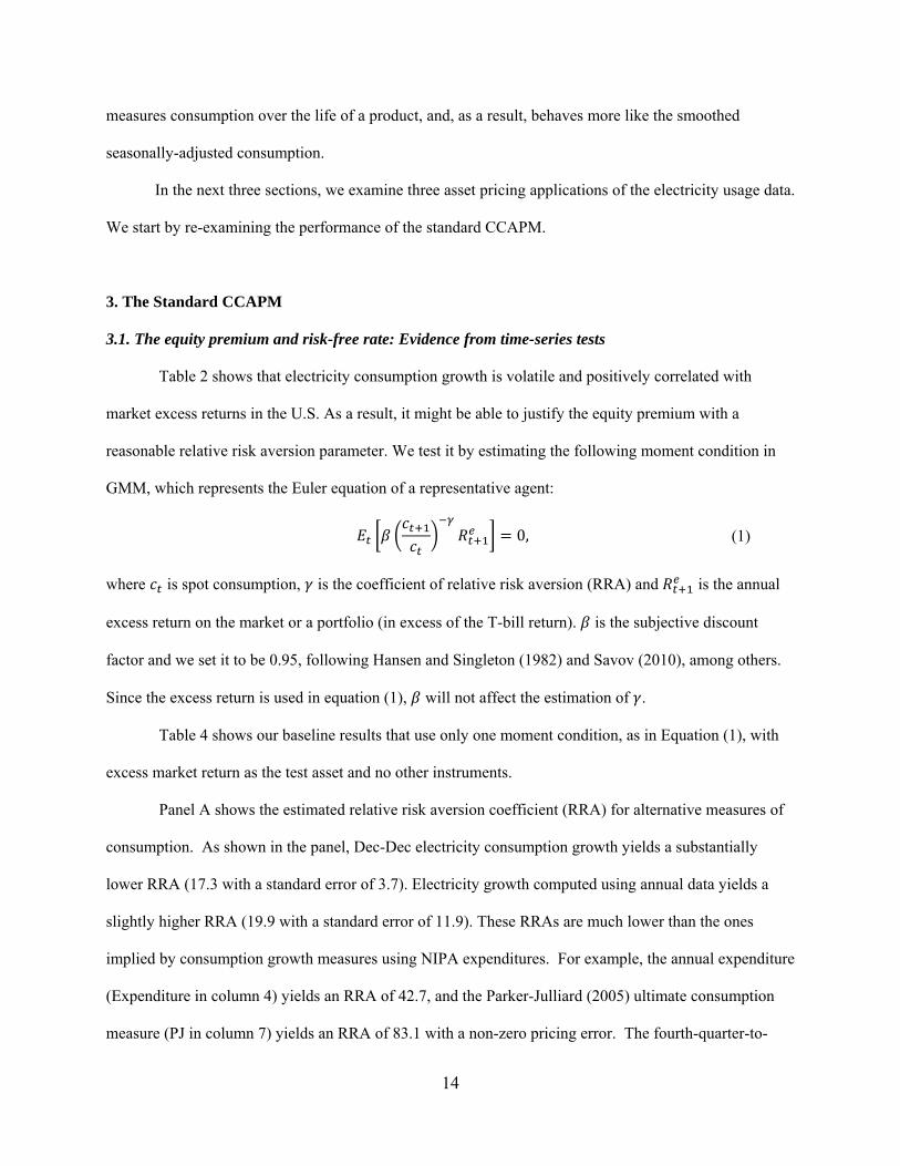
Table 2 shows that electricity consumption growth is volatile and positively correlated with
market excess returns in the U.S. As a result, it might be able to justify the equity premium with a
reasonable relative risk aversion parameter. We test it by estimating the following moment condition in
GMM, which represents the Euler equation of a representative agent:
0, (1)
where is spot consumption, is the coefficient of relative risk aversion (RRA) and is the annual
excess return on the market or a portfolio (in excess of the T-bill return). is the subjective discount
factor and we set it to be 0.95, following Hansen and Singleton (1982) and Savov (2010), among others.
Since the excess return is used in equation (1), will not affect the estimation of .
Table 4 shows our baseline results that use only one moment condition, as in Equation (1), with
excess market return as the test asset and no other instruments.
Panel A shows the estimated relative risk aversion coefficient (RRA) for alternative measures of
consumption. As shown in the panel, Dec-Dec electricity consumption growth yields a substantially
lower RRA (17.3 with a standard error of 3.7). Electricity growth computed using annual data yields a
slightly higher RRA (19.9 with a standard error of 11.9). These RRAs are much lower than the ones
implied by consumption growth measures using NIPA expenditures. For example, the annual expenditure
(Expenditure in column 4) yields an RRA of 42.7, and the Parker-Julliard (2005) ultimate consumption
measure (PJ in column 7) yields an RRA of 83.1 with a non-zero pricing error. The fourth-quarter-to-
15
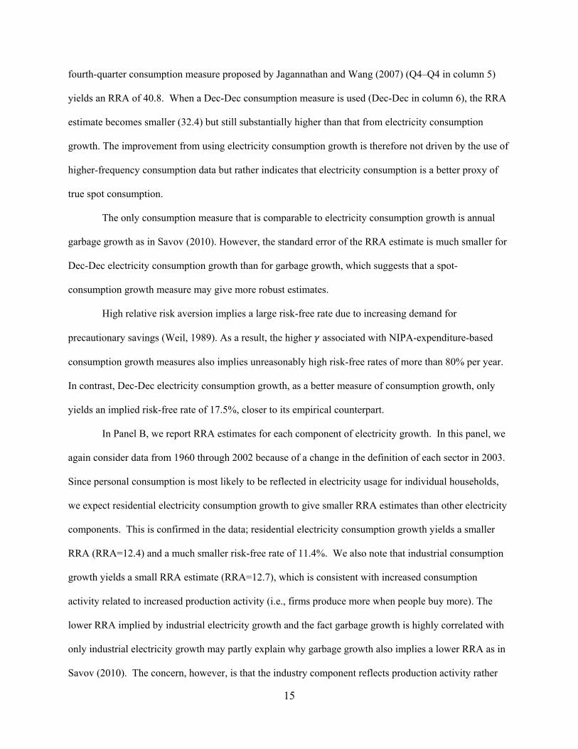
fourth-quarter consumption measure proposed by Jagannathan and Wang (2007) (Q4–Q4 in column 5)
yields an RRA of 40.8. When a Dec-Dec consumption measure is used (Dec-Dec in column 6), the RRA
estimate becomes smaller (32.4) but still substantially higher than that from electricity consumption
growth. The improvement from using electricity consumption growth is therefore not driven by the use of
higher-frequency consumption data but rather indicates that electricity consumption is a better proxy of
true spot consumption.
The only consumption measure that is comparable to electricity consumption growth is annual
garbage growth as in Savov (2010). However, the standard error of the RRA estimate is much smaller for
Dec-Dec electricity consumption growth than for garbage growth, which suggests that a spot-
consumption growth measure may give more robust estimates.
High relative risk aversion implies a large risk-free rate due to increasing demand for
precautionary savings (Weil, 1989). As a result, the higher associated with NIPA-expenditure-based
consumption growth measures also implies unreasonably high risk-free rates of more than 80% per year.
In contrast, Dec-Dec electricity consumption growth, as a better measure of consumption growth, only
yields an implied risk-free rate of 17.5%, closer to its empirical counterpart.
In Panel B, we report RRA estimates for each component of electricity growth. In this panel, we
again consider data from 1960 through 2002 because of a change in the definition of each sector in 2003.
Since personal consumption is most likely to be reflected in electricity usage for individual households,
we expect residential electricity consumption growth to give smaller RRA estimates than other electricity
components. This is confirmed in the data; residential electricity consumption growth yields a smaller
RRA (RRA=12.4) and a much smaller risk-free rate of 11.4%. We also note that industrial consumption
growth yields a small RRA estimate (RRA=12.7), which is consistent with increased consumption
activity related to increased production activity (i.e., firms produce more when people buy more). The
lower RRA implied by industrial electricity growth and the fact garbage growth is highly correlated with
only industrial electricity growth may partly explain why garbage growth also implies a lower RRA as in
Savov (2010). The concern, however, is that the industry component reflects production activity rather
16
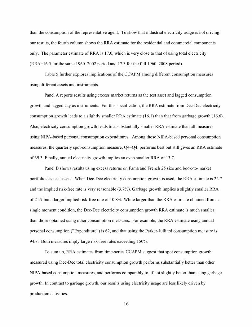
than the consumption of the representative agent. To show that industrial electricity usage is not driving
our results, the fourth column shows the RRA estimate for the residential and commercial components
only. The parameter estimate of RRA is 17.0, which is very close to that of using total electricity
(RRA=16.5 for the same 1960–2002 period and 17.3 for the full 1960–2008 period).
Table 5 further explores implications of the CCAPM among different consumption measures
using different assets and instruments.
Panel A reports results using excess market returns as the test asset and lagged consumption
growth and lagged cay as instruments. For this specification, the RRA estimate from Dec-Dec electricity
consumption growth leads to a slightly smaller RRA estimate (16.1) than that from garbage growth (16.6).
Also, electricity consumption growth leads to a substantially smaller RRA estimate than all measures
using NIPA-based personal consumption expenditures. Among those NIPA-based personal consumption
measures, the quarterly spot-consumption measure, Q4–Q4, performs best but still gives an RRA estimate
of 39.3. Finally, annual electricity growth implies an even smaller RRA of 13.7.
Panel B shows results using excess returns on Fama and French 25 size and book-to-market
portfolios as test assets. When Dec-Dec electricity consumption growth is used, the RRA estimate is 22.7
and the implied risk-free rate is very reasonable (3.7%). Garbage growth implies a slightly smaller RRA
of 21.7 but a larger implied risk-free rate of 10.8%. While larger than the RRA estimate obtained from a
single moment condition, the Dec-Dec electricity consumption growth RRA estimate is much smaller
than those obtained using other consumption measures. For example, the RRA estimate using annual
personal consumption (”Expenditure”) is 62, and that using the Parker-Julliard consumption measure is
94.8. Both measures imply large risk-free rates exceeding 150%.
To sum up, RRA estimates from time-series CCAPM suggest that spot consumption growth
measured using Dec-Dec total electricity consumption growth performs substantially better than other
NIPA-based consumption measures, and performs comparably to, if not slightly better than using garbage
growth. In contrast to garbage growth, our results using electricity usage are less likely driven by
production activities.

17
3.2. Evidence from the cross section
Another key insight of the CCAPM is that an asset’s consumption beta – covariance between
asset return and aggregate consumption growth – determines its expected return. This can be easily seen
by linearizing the Euler equation of (1) as in Jagannathan and Wang (2007) and Savov (2010):
, . (2)
In this subsection, we test this cross-sectional implication of the CCAPM by running Fama-
MacBeth (1973) regressions. Specifically, we first regress a portfolio’s excess returns on various
measures of consumption growth in a time-series regression to obtain the consumption beta of that
portfolio. We then run cross-sectional regressions of portfolio excess returns on their consumption betas.
We choose the 25 Fama-French size and book-to-market portfolios which are the standard test assets for
cross-sectional asset pricing. We first follow Savov (2010) and omit the intercept terms in the cross-
sectional regressions. According to Savov (2010), omitting the intercept imposes a restriction of the
model and delivers more power. The results of these regressions are reported in Panel A of Table 6. In
Panel B, we also report results after including intercept terms in the cross-sectional regressions which is a
more standard procedure (see Lettau and Ludvigson (2001) and Jagannathan and Wang (2007) among
many others).
For each regression specification, the regression coefficients are reported in the first row; Fama-
MacBeth t-values with Newey-West (1987) correction are reported in the second row; t-values with both
Shanken (1992) and Newey-West corrections are reported in the third row. The Shanken correction
accounts for the estimation errors in betas from the time-series regressions and the Newey-West
correction accounts for autocorrelations in the errors with a lag of 3. The sampling period is again from
1961 to 2007.
The first two regressions in Panel A show that when there is no intercept term in the cross-
sectional regression, both Dec-Dec electricity growth (eg) and the standard NIPA expenditure growth (cg)
18
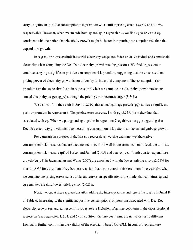
carry a significant positive consumption risk premium with similar pricing errors (3.05% and 3.07%,
respectively). However, when we include both eg and cg in regression 3, we find eg to drive out cg,
consistent with the notion that electricity growth might be better in capturing consumption risk than the
expenditure growth.
In regression 4, we exclude industrial electricity usage and focus on only residual and commercial
electricity when computing the Dec-Dec electricity growth rate (eg_rescom). We find eg_rescom to
continue carrying a significant positive consumption risk premium, suggesting that the cross-sectional
pricing power of electricity growth is not driven by its industrial component. The consumption risk
premium remains to be significant in regression 5 when we compute the electricity growth rate using
annual electricity usage (eg_A) although the pricing error becomes larger (3.74%).
We also confirm the result in Savov (2010) that annual garbage growth (gg) carries a significant
positive premium in regression 6. The pricing error associated with gg (3.33%) is higher than that
associated with eg. When we put gg and eg together in regression 7, eg drives out gg, suggesting that
Dec-Dec electricity growth might be measuring consumption risk better than the annual garbage growth.
For comparison purpose, in the last two regressions, we also examine two alternative
consumption risk measures that are documented to perform well in the cross-section. Indeed, the ultimate
consumption risk measure (pj) of Parker and Julliard (2005) and year-on-year fourth quarter expenditure
growth (cg_q4) in Jagannathan and Wang (2007) are associated with the lowest pricing errors (2.56% for
pj and 1.88% for cg_q4) and they both carry a significant consumption risk premium. Interestingly, when
we compare the pricing errors across different regression specifications, the model that combines eg and
cg generates the third lowest pricing error (2.62%).
Next, we repeat these regressions after adding the intercept terms and report the results in Panel B
of Table 6. Interestingly, the significant positive consumption risk premium associated with Dec-Dec
electricity growth (eg and eg_rescom) is robust to the inclusion of an intercept term in the cross-sectional
regression (see regression 1, 3, 4, and 7). In addition, the intercept terms are not statistically different
from zero, further confirming the validity of the electricity-based CCAPM. In contrast, expenditure
19
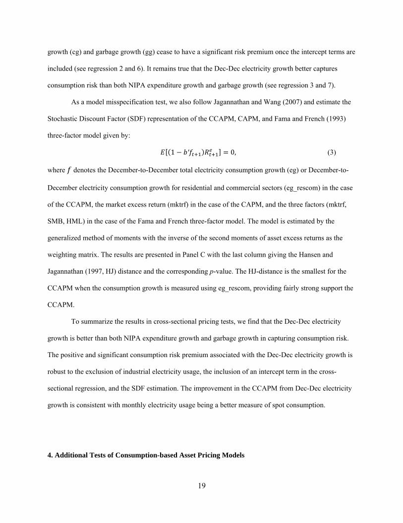
growth (cg) and garbage growth (gg) cease to have a significant risk premium once the intercept terms are
included (see regression 2 and 6). It remains true that the Dec-Dec electricity growth better captures
consumption risk than both NIPA expenditure growth and garbage growth (see regression 3 and 7).
As a model misspecification test, we also follow Jagannathan and Wang (2007) and estimate the
Stochastic Discount Factor (SDF) representation of the CCAPM, CAPM, and Fama and French (1993)
three-factor model given by:
1 ′ 0, (3)
where denotes the December-to-December total electricity consumption growth (eg) or December-to-
December electricity consumption growth for residential and commercial sectors (eg_rescom) in the case
of the CCAPM, the market excess return (mktrf) in the case of the CAPM, and the three factors (mktrf,
SMB, HML) in the case of the Fama and French three-factor model. The model is estimated by the
generalized method of moments with the inverse of the second moments of asset excess returns as the
weighting matrix. The results are presented in Panel C with the last column giving the Hansen and
Jagannathan (1997, HJ) distance and the corresponding p-value. The HJ-distance is the smallest for the
CCAPM when the consumption growth is measured using eg_rescom, providing fairly strong support the
CCAPM.
To summarize the results in cross-sectional pricing tests, we find that the Dec-Dec electricity
growth is better than both NIPA expenditure growth and garbage growth in capturing consumption risk.
The positive and significant consumption risk premium associated with the Dec-Dec electricity growth is
robust to the exclusion of industrial electricity usage, the inclusion of an intercept term in the cross-
sectional regression, and the SDF estimation. The improvement in the CCAPM from Dec-Dec electricity
growth is consistent with monthly electricity usage being a better measure of spot consumption.
4. Additional Tests of Consumption-based Asset Pricing Models

20
4.1. Calendar cycle effect in consumption: U.S. and European evidence
In Table 7, we examine the year-on-year total electricity consumption growth over different
calendar cycle in the context of the standard CCAPM. In Panel A, we report RRA estimates using year-
on-year total electricity consumption growth for each month in U.S. During the first four months of the
year, the Euler equation in (1) does not hold on average and the resulting RRA estimates are not very
meaningful. From May to December, the Euler equation holds and Dec-Dec electricity consumption
growth yields the lowest RRA; the Dec-Dec RRA estimate is also associated with the smallest standard
error.
There are at least two reasons why Dec-Dec electricity consumption growth might perform better
in the CCAPM. First, as shown in row 5, electricity consumption is affected by weather conditions.
Specifically, weather impacts are stronger in summer months due to increased cooling demand. Weather
impact is measured by the correlation between monthly weather shock and total electricity consumption.
The monthly weather shock is measured by the deviation of monthly energy degree days (EDD) which is
in turn the sum of annual cooling degree days (CDD) and annual heating degree days (HDD). CDD
(absolute value of temperature minus 65oF) and HDD (absolute value of 65oF minus temperature) are
conventional measures of weather-driven electricity demand and are obtained from the National Oceanic
and Atmospheric Administration (NOAA). During the three months from June to August, extreme
weather variation drives year-on-year electricity consumption growth. In contrast, November and
December year-on-year electricity consumption growth rates are much less affected by the weather
change. As a result, Dec-Dec electricity consumption growth may be more informative about the true spot
consumption growth. Second, as argued in Jagannathan and Wang (2007), December, in the U.S.,
coincides with both the end of the tax year and the winter holiday. This is the time when investors both
feel the need and have more leisure time to review their consumption and portfolio choice decisions, and
consequently, the CCAPM should perform better.
We then examine a similar calendar cycle effect in European countries. This exercise also helps
to further confirm the usefulness of total electricity consumption growth as a spot measure of
21
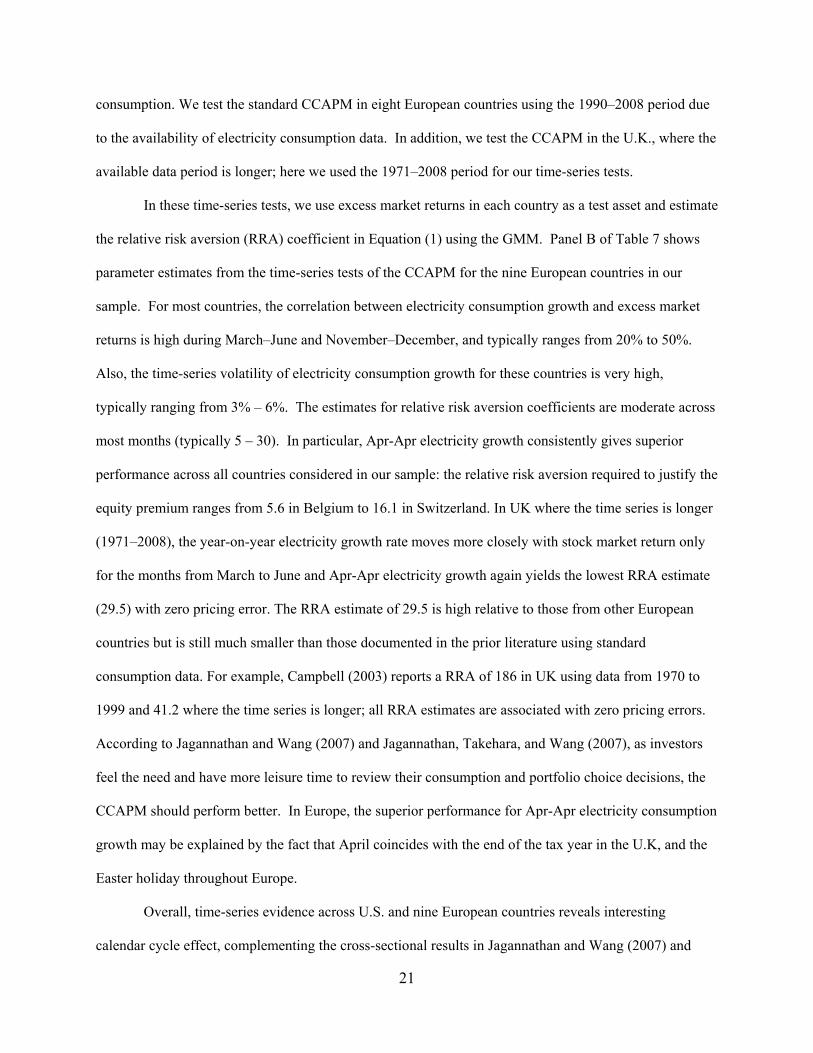
consumption. We test the standard CCAPM in eight European countries using the 1990–2008 period due
to the availability of electricity consumption data. In addition, we test the CCAPM in the U.K., where the
available data period is longer; here we used the 1971–2008 period for our time-series tests.
In these time-series tests, we use excess market returns in each country as a test asset and estimate
the relative risk aversion (RRA) coefficient in Equation (1) using the GMM. Panel B of Table 7 shows
parameter estimates from the time-series tests of the CCAPM for the nine European countries in our
sample. For most countries, the correlation between electricity consumption growth and excess market
returns is high during March–June and November–December, and typically ranges from 20% to 50%.
Also, the time-series volatility of electricity consumption growth for these countries is very high,
typically ranging from 3% – 6%. The estimates for relative risk aversion coefficients are moderate across
most months (typically 5 – 30). In particular, Apr-Apr electricity growth consistently gives superior
performance across all countries considered in our sample: the relative risk aversion required to justify the
equity premium ranges from 5.6 in Belgium to 16.1 in Switzerland. In UK where the time series is longer
(1971–2008), the year-on-year electricity growth rate moves more closely with stock market return only
for the months from March to June and Apr-Apr electricity growth again yields the lowest RRA estimate
(29.5) with zero pricing error. The RRA estimate of 29.5 is high relative to those from other European
countries but is still much smaller than those documented in the prior literature using standard
consumption data. For example, Campbell (2003) reports a RRA of 186 in UK using data from 1970 to
1999 and 41.2 where the time series is longer; all RRA estimates are associated with zero pricing errors.
According to Jagannathan and Wang (2007) and Jagannathan, Takehara, and Wang (2007), as investors
feel the need and have more leisure time to review their consumption and portfolio choice decisions, the
CCAPM should perform better. In Europe, the superior performance for Apr-Apr electricity consumption
growth may be explained by the fact that April coincides with the end of the tax year in the U.K, and the
Easter holiday throughout Europe.
Overall, time-series evidence across U.S. and nine European countries reveals interesting
calendar cycle effect, complementing the cross-sectional results in Jagannathan and Wang (2007) and

22
Jagannathan, Takehara, and Wang (2007). The European evidence also provides additional out-of-sample
support for our electricity-based CCAPM.
4.2. Incomplete market model: Evidence from state-level data
A popular alternative for explaining the equity risk premium puzzle is to relax the complete
market assumption and allow heterogeneous agents to have uninsurable income shocks (see
Constantinides and Duffie (1996) and Constantinides (2002) among many others). After relaxing the
representative-agent assumption, the Euler equation (1) now holds for each consumer , or:
,
,0. (4)
Aggregating the Euler equations across consumers in the economy, we have a new Euler equation:
1 ,
,0, (5)
Following Jacobs, Pallage and Robe (2005) and Korniotis (2008), we test equation (4) not using
data on individual consumption, but data on state consumption. State-level consumption data alleviates
measurement error associated with individual consumption data sets such as the Consumer Expenditure
Survey and the Panel Study of Income Dynamics. In addition, it can be interpreted as a proxy for the
consumption of a synthetic cohort as studied by Browning, Deaton, and Irish (1985) and Attanasio and
Weber (1995). Jacobs, Pallage and Robe (2005) and Korniotis (2008) measure annual state-level
consumption using retail sales data. In contrast, we measure annual state-level consumption using annual
state-level total electricity usage. In other words, in equation (3) is measured using per capita annual
electricity usage in state . When we aggregate across states, we consider both the equally-weighted
average as in equation (4) and the population-weighted average. We use annual state electricity usage as
the data goes back to 1960 while monthly state-level electricity usage data only becomes available in
1990.
23
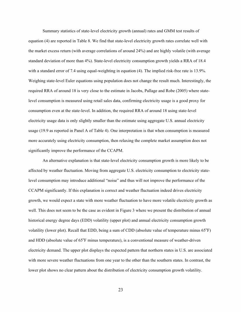
Summary statistics of state-level electricity growth (annual) rates and GMM test results of
equation (4) are reported in Table 8. We find that state-level electricity growth rates correlate well with
the market excess return (with average correlations of around 24%) and are highly volatile (with average
standard deviation of more than 4%). State-level electricity consumption growth yields a RRA of 18.4
with a standard error of 7.4 using equal-weighting in equation (4). The implied risk-free rate is 13.9%.
Weighing state-level Euler equations using population does not change the result much. Interestingly, the
required RRA of around 18 is very close to the estimate in Jacobs, Pallage and Robe (2005) where state-
level consumption is measured using retail sales data, confirming electricity usage is a good proxy for
consumption even at the state-level. In addition, the required RRA of around 18 using state-level
electricity usage data is only slightly smaller than the estimate using aggregate U.S. annual electricity
usage (19.9 as reported in Panel A of Table 4). One interpretation is that when consumption is measured
more accurately using electricity consumption, then relaxing the complete market assumption does not
significantly improve the performance of the CCAPM.
An alternative explanation is that state-level electricity consumption growth is more likely to be
affected by weather fluctuation. Moving from aggregate U.S. electricity consumption to electricity state-
level consumption may introduce additional “noise” and thus will not improve the performance of the
CCAPM significantly. If this explanation is correct and weather fluctuation indeed drives electricity
growth, we would expect a state with more weather fluctuation to have more volatile electricity growth as
well. This does not seem to be the case as evident in Figure 3 where we present the distribution of annual
historical energy degree days (EDD) volatility (upper plot) and annual electricity consumption growth
volatility (lower plot). Recall that EDD, being a sum of CDD (absolute value of temperature minus 65oF)
and HDD (absolute value of 65oF minus temperature), is a conventional measure of weather-driven
electricity demand. The upper plot displays the expected pattern that northern states in U.S. are associated
with more severe weather fluctuations from one year to the other than the southern states. In contrast, the
lower plot shows no clear pattern about the distribution of electricity consumption growth volatility.

24
Overall, while weather fluctuation is positively correlated with electricity growth volatility across states
(correlation is about 10%), electricity growth does not seem to be driven by weather fluctuation.
More importantly, we directly test the impact of weather fluctuation on our time-series tests and
report the results in Panel B of Table 8. We classify 48 states with non-missing EDD measures into two
groups according to their annual EDD volatility.8 As seen from Figure 3, the 24 states in the high-EDD-
volatility group are mainly the northern states while the 24 states in the low-EDD-volatility group are
mainly the southern states. We then test the main Euler equation at both aggregate level (equation 1) and
at the state-level (equation 4 with population-weighting) within each of the two groups. The results in the
two groups turn out to be very similar, confirming that weather fluctuation has little impact on the asset
pricing results in this paper.
5. Stock Return Predictability
Preceding sections consider electricity consumption growth as a measure of consumption risk of a
representative investor. In the U.S., electricity consumption data are available across three broad sectors
of the economy including households (residential electricity usage), commercial businesses (commercial
electricity usage), and industrial firms (industrial electricity usage). While residential and commercial
electricity usage has been shown to be a good measure of the representative agent’s consumption, in this
section, we explore the possibility of using industrial electricity usage as an economic indicator that
forecasts future stock returns.
Since factories typically use electricity in their production and electricity cannot be stored,
industrial electricity usage is likely to track production, economic output and hence business cycle
fluctuation in real time. In Panel A of Table 9, we report the simple correlations between various
consumption risk variables and an annual NBER business cycle variable defined as the fraction of each
year spent in non-recession. As shown in the table, December-to-December industrial electricity
consumption growth has the highest correlation (57%). The only other growth variable that has 8 The three states with missing EDDs are Alaska, Hawaii and Washington DC.
25
comparable correlation (55%) with the NBER business cycle variable is the Q4-Q4 NIPA consumption
growth as in Jagannathan and Wang (2007).
It is important to highlight that the NBER recession dates are often announced with significant
delay. Industrial electricity usage, available with minimum delay, could capture business cycle on a
timely basis. If the market risk premium is countercyclical as predicted by theoretical models such as
Campbell and Cochrane (1999), then our industrial electricity growth rate could be a good predictor of
future stock excess returns. We test this conjecture using time series regressions following the standard
procedures in the return predictability literature (see Goyal and Welch (2008) for a comprehensive study
of return predictability). Specifically, we consider the following predictive regression:
, (6)
where is next year stock excess return, is current year predictive variable, and is a random
noise. For excess returns, we consider the CRSP value-weighted market returns over T-bill rates, and
Fama-French 12 industry returns over T-bill rates. Predictive variables are December-to-December
growth rate in components of electricity usage (residential, commercial, industrial, and total), book-to-
market ratio (b/m), investment to capital ratio (i/k), net equity expansion (ntis), percent equity issuing
(eqis), consumption wealth ratio (cay), dividend yield (dy), earnings price ratio (ep), annual garbage
growth rate of Savov (2010) (gg), and year-on-year fourth quarter expenditure growth by Jagannathan and
Wang (2007) (cg_q4). We choose to include b/m, i/k, ntis, eqis, cay, dy, and ep since Goyal and Welch
(2008) find them to have significant predictive power among a comprehensive list of predictive variables
they studied. We compute boostrap p-values associated with the regression estimates following the
procedure detailed in Goyal and Welch (2008). These boostrap p-values account for the persistence in the
predictor, cross-correlation in the error terms and the small-sample problem. We examine predictive
variables in the sample period 1960–2002 due to a change in the definition of electricity usage sector in
2003. If we ignore this “structure break” extend our sampling period to 2008, unreported results suggest
our industrial electricity growth to perform even better. Given the relatively short sampling period, we do
not compute the out-of-sample R2.
26
In Panel B, Table 9, we report results from the predictive regressions for next-year excess market
returns. As shown in Panel B, the parameter estimate on December-to-December industrial electricity
consumption growth is significantly negative. That is, lower industrial electricity growth in the current
period forecasts higher excess returns over the following year, consistent with a countercyclical premium
so the market risk premium increases during an economic downturn. The R2 for this regression is 9.68%
which is also highly significant. Among other variables considered in Goyal and Welch (2008), only
percent equity issuing (eqis) and the consumption-wealth ratio (cay) have higher R2 (10.66% and 22.82%).
While eqis is computed using price information and cay is calculated via forward-looking full sample
estimation, our industrial electricity growth variable is purely quantity-based and does not require any
full-sample estimation.
Panel B also shows that another consumption growth measure (cg_q4) does a reasonably good
job in predicting next-year market excess returns (albeit not as good as our industrial electricity growth in
our sampling period 1960-2002). The good performance of cg_q4 in predicting future market excess
returns confirms the recent findings by Moller and Rangvid (2010) and is consistent with the high
correlation between cg_q4 and the NBER business cycle variable documented in Panel A.
In Panel C, Table 9, we further examine industry-level predictability using Fama-French 12
industry portfolios. To save space, we only consider the top three predictive variables: our industrial
electricity growth, eqis, and cay. Among 12 industries, nondurable (R2=19.2%), durable (R2=17.5%),
manufacturing (R2=14.3%), chemical (R2=17.9%), shops (R2=20.5%), and money (R2=17.1%) industry
excess returns are well predicted by industrial electricity consumption growth with significant parameter
estimates and high R2. Using eqis and cay, we find similar predictability patterns that excess returns in
nondurable, durable, manufacturing, chemical, shops, and money industries are well predicted. In terms
of predictability R2, industrial electricity consumption growth has better predictive power than percent
equity issuing (eqis) for most industries, and has similar predictive power as the consumption-wealth ratio
(cay).
27
If countercyclical market risk premium is behind the predictive relation between current industrial
electricity consumption growth and future stock excess returns, we would expect strong predictive power
among industries with higher exposures to systematic risk (see Rapach, Strauss, Tu, and Zhou (2010) for
a similar argument). Figure 4 provides consistent evidence supporting this conjecture. We plot the R2
from the predictive regressions (using industrial electricity growth) across the 12 industries against each
of the three factor betas across the 12 industries (MKTRF betas in panel (a), SMB betas in panel (b) and
HML betas in panel (c)). As shown in these figures, predictive R2s are indeed positively correlated with
all three betas.
While a more extensive investigation of the predictive power of electricity consumption growth
warrants a separate study, the results in this section do suggest that electricity consumption growth is a
useful economic indicator in forecasting future asset returns.
6. Conclusions
In this paper, we propose electricity consumption growth as a new real-time measure of economic
activities such as aggregate spot consumptions and business cycle fluctuations. This is because most
modern-day economic activities involve the use of electricity, which cannot be easily stored. The
availability of high frequency data at both aggregate and disaggregate level permits us to examine the link
between economic activities and asset prices. We find that electricity usage can better explain stock
returns in both time-series and cross-section within the consumption-based asset pricing framework. It is
also capable of capturing business cycle fluctuations and predicts future stock excess returns well.
In the U.S. from 1961 to 2008, electricity consumption growth is able to match the equity
premium with a relative risk aversion of 17.3, which is much lower than those associated with the NIPA
expenditure growth measures. In the cross section, we find a positive and significant consumption risk
premium using Dec-Dec annual electricity growth rates. In addition, our results are not driven by
electricity demand coming from production activities and extreme weather fluctuations.

28
Electricity usage data is available at disaggregated level, higher frequency and almost in real time,
which allows us to study additional implications of consumption in asset pricing. We examine two such
implications in our paper. We test the calendar effect associated with aggregate consumption using
monthly electricity data and we test the CCAPM with incomplete market and uninsurable income shocks
using state-level electricity data.
Finally, we show that December-to-December industrial electricity growth captures business
cycle variations well and has a high correlation of 57% with an annual NBER business cycle variable.
This property leads to good performance in predicting future stock excess returns at both market and
industry level with an in-sample R2 of 9.7% for future excess market returns and of 20% for industry
excess returns for several industries (such as Consumer, Non-durables, and Shops).
Beyond establishing a strong link between fundamental economic activities and asset prices, our
paper also illustrates the usefulness of the electricity consumption data in financial applications. High-
frequency real time electricity usage data points to further applications in areas where accurate timing is
an important issue. We leave them for future studies.

29
References
Abel, Andrew B., Janice C. Eberly, and Stavros Panageas. 2007. “Optimal Inattention to the
Stock Market.” American Economic Review, 97(2): 244–249.
Ait-Sahalia, Yacine, Jonathan A. Parker, and Motohiro Yogo. 2004. “Luxury Goods and the
Equity Premium.” Journal of Finance 59:2959–3004.
Attanasio Orazio P., and Guglielmo Weber. 1995. “Is Consumption Growth Consistent with
Intertemporal Optimization? Evidence from the Consumer Expenditure Survey.” Journal of Political
Economy 103:1121–1157.
Bansal, Ravi, and Amir Yaron. 2004. “Risks for the Long Run: A Potential Resolution of Asset
Pricing Puzzles.” Journal of Finance 59:1481–1509.
Breeden, Douglas T. 1979. “An Intertemporal Asset Pricing Model with Stochastic Consumption
and Investment Opportunities.” Journal of Financial Economics 7:265–296.
Breeden, Douglas T., Michael Gibbons, and Robert Litzenberger. 1989. “Empirical Test of the
Consumption Oriented CAPM.” Journal of Finance 44: 231–262.
Browning, Martin, Angus Deaton, and Margaret Irish. 1985. “A Profitable Approach to Labor
Supply and Commodity Demands over the Life-Cycle.” Econometrica 53:503–544.
Campbell, John Y. 1999. “Asset Prices, Consumption, and the Business Cycle.” Vol 1, Part 3 of
Handbook of Macroeconomics pp.1231–1303.
Campbell, John Y. 2003. “Consumption-based Asset Pricing.” Chapter 13 of Handbook of the
Economics of Finance, pp.801-885.
Campbell, John Y., and John H. Cochrane. 1999. “By Force of Habit: A Consumption-Based
Explanation of Aggregate Stock Market Behavior.” Journal of Political Economy 107:205–251.
Cochrane, John H. 2007. “The Dog That Did Not Bark: A Defense of Return Predictability.”
Review of Financial Studies 21:1533–1575.
Comin, Diego, and Mark Gertler. 2006. “Medium-Term Business Cycle” American Economic
Review 96(3):523–551.
30
Constantinides, George M. 1990. “Habit Formation: A Resolution of the Equity Premium Puzzle.”
Journal of Political Economy 98:519–543.
Constantinides, George M. 2002. “Rational Asset Prices.” Journal of Finance 57:1567–1591.
Constantinides, George M., John B. Donaldson, and Rajnish Mehra. 2002. “Junior Can’t Borrow:
A New Perspective on the Equity Premium Puzzle.” Quarterly Journal of Economics 117:269–296.
Constantinides, George M., and Darrell Duffie. 1996. “Asset Pricing with Heterogeneous
Consumers.” Journal of Political Economy 104:219–240.
Epstein, Larry G., and Stanley E. Zin. 1991. “Substitution, Risk Aversion, and the Temporal
Behavior of Consumption and Asset Returns: An Empirical Analysis.” Journal of Political Economy
96:263–286.
Fama, Eugene F., and Kenneth R. French. 1992. “The Cross-Section of Expected Stock Returns.”
Journal of Finance 47:427–465.
Fama, Eugene F., and Kenneth R. French. 1993. “Common Factors in the Returns on Stocks and
Bonds.” Journal of Financial Economics 33:3–56.
Fama, Eugene F, and James D MacBeth. 1973. “Risk, Return, and Equilibrium: Empirical Tests.”
Journal of Political Economy 81:607–636.
Ferson, Wayne E., and Campbell R. Harvey. 1992. “Seasonality and Consumption-Based Asset
Pricing.” Journal of Finance 47:511–551.
Goyal, Amit, and Ivo Welch. 2008. “A Comprehensive Look at The Empirical Performance of
Equity Premium Prediction.” Review of Financial Studies 21:1455–1508.
Hall, Robert E. 1978. “Stochastic Implications of the Life Cycle-Permanent Income Hypothesis:
Theory and Evidence.” Journal of Political Economy 86:971–987.
Hansen, Lars Peter, John C. Heaton, and Nan Li. 2008. “Consumption Strikes Back? Measuring
Long-Run Risk.” Journal of Political Economy 116:260–302.
Hansen, Lars Peter, and Jagannathan, Ravi. 1997. “Assessing Specification Errors in Stochastic
Discount Factor Models.” Journal of Finance 52:557–590.
31
Hansen, Lars Peter, and Kenneth J. Singleton. 1982. “Generalized Instrumental Variables
Estimation of Nonlinear Rational Expectations Models.” Econometrica 50:1269–1286.
Jacobs, Kris, Stephane Pallage, and Michel A. Robe. 2005. “Market Incompleteness and the
Equity Premium Puzzle: Evidence from State-Level Data.” Working Paper, McGill University.
Jagannathan, Ravi, Hitoshi Takehara, and Yong Wang. 2007. “Calendar Cycles, Infrequent
Decisions and the Cross-Section of Stock Returns.” Working Paper, Northwestern University.
Jagannathan, Ravi, and Yong Wang. 2007. “Lazy Investors, Discretionary Consumption, and the
Cross-Section of Stock Returns.” Journal of Finance 62:1623–1661.
Korniotis, George M. 2008. “Habit Formation, Incomplete Markets, and the Significance of
Regional Risk for Expected Returns.” Review of Financial Studies 21:2139–2172.
Lettau, Martin, and Sydney Ludvigson. 2001. “Resurrecting the (C)CAPM: A Cross-Sectional
Test When Risk Premia Are Time-Varying.” Journal of Political Economy 109:1238–1287.
Lettau, Martin, and Sydney Ludvigson. 2009. “Measuring and Modeling Variation in the Risk-
Return Tradeoff.” Handbook of Financial Econometrics, forthcoming.
Lucas, Robert E, Jr. 1978. “Asset Prices in An Exchange Economy.” Econometrica 46:1429–
1445.
Malloy, Christopher J., Tobias J. Moskowitz, and Annette Vissing-Jorgensen. 2009. “Long-Run
Stockholder Consumption Risk and Asset Returns.” Journal of Finance 69:2427–2479.
Mankiw, N. Gregory, and Stephen P. Zeldes. 1991. “The Consumption of Stockholders and
Nonstockholders.” Journal of Financial Economics 29:97–112.
Mehra, Rajnish., and Edward C. Prescott. 1985. “The Equity Premium: A Puzzle.” Journal of
Monetary Economics 15:145–161.
Moller, Stig V., and Jesper Rangvid. 2010. “The Fourth-Quarter Consumption Growth Rate: A
Pure-Macro, Not-Estimated Stock Return Predictor That Works In-Sample and Out-Of-Sample.”
Working Paper,. Aarhus University.

32
Newey, Whitney K., and Kenneth D. West. 1987. “A Simple, Positive Semi-Definite,
Heteroskedasticity and Autocorrelation Consistent Covariance Matrix.” Econometrica 55:703–708.
Parker, Jonathan A., and Christian Julliard. 2005. “Consumption Risk and the Cross Section of
Expected Returns.” Journal of Political Economy 113:185–222.
Rapach, David E., Jack K. Strauss, Jun Tu, Guofu Zhou. 2010. “Industry Return Predictability: Is
It There Out of Sample?” working Paper, Washington University in St.Louis.
Savov, Alexi. 2010. “Asset Pricing with Garbage.” Journal of Finance, Forthcoming.
Shanken, Jay. 1992. “On the Estimation of Beta Pricing Models.” Review of Financial Studies
5:1–33.
Sundaresan, Suresh M. 1989. “Intertemporally Dependent Preferences and the Volatility of
Consumption and Wealth.” Review of Financial Studies 2:73–89.
Weil, Philippe. 1989. “The Equity Premium Puzzle and the Risk-Free Rate Puzzle.” Journal of
Monetary Economics 24:401–422.
33
Table 1 Summary statistics: Components of electricity consumption growth Information on monthly sales of electric energy to ultimate customers is collected from the Energy Information Administration’s (EIA) Electric Power Statistics (1960–1978) and Electric Power Monthly (1979–2008). Electricity growth is measured by year-on-year December electricity consumption growth by sector. Sector-level results consider 1960–2002 data due to a change in the definition of each sector in 2003. According to EIA Form 826, residential sector consists of living quarters for private households. Commercial sector consists of service-providing facilities and equipment of business; Federal, State, and local governments; and other private and public organizations, such as religious, social, or fraternal groups. Industrial sector consists of all facilities and equipment used for producing, processing or assembling goods. The following types of activities are included in the industrial sector: manufacturing (NAICS codes 31-33); agriculture, forestry, and hunting (NAICS code 11); mining, including oil and gas extraction (NAICS code 21); natural gas distribution (NAICS code 2212); and construction (NAICS code 23). Aside from residential, commercial, and industrial sectors, other electricity consumption activities such as public street and highway lighting, other sales to public authorities, sales to railroads and railways, sales for irrigation, and interdepartmental sales are also included in the total electricity consumption. In the fourth row, excess market returns are measured by value weighted U.S. stock returns over one-month Treasury bill returns. Residential Commercial Industrial Res & Com Total Proportion (%) 33.5 25.1 37.9 58.6 100.0 Mean 1.034 1.041 1.017 1.048 1.029 Std. dev. (%) 5.9 3.4 6.0 4.6 4.4 Corr. with Rm (%) 10.2 23.6 33.3 16.7 27.3
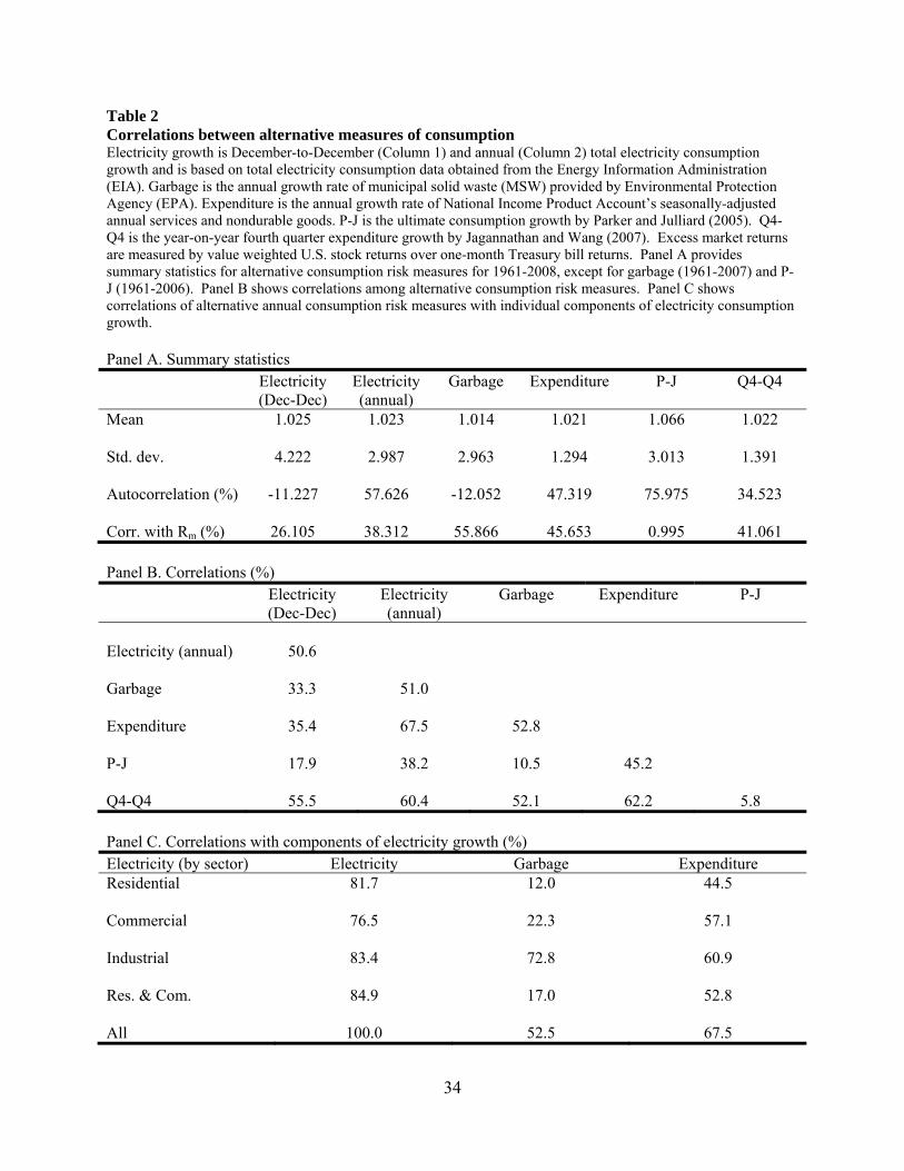
34
Table 2 Correlations between alternative measures of consumption Electricity growth is December-to-December (Column 1) and annual (Column 2) total electricity consumption growth and is based on total electricity consumption data obtained from the Energy Information Administration (EIA). Garbage is the annual growth rate of municipal solid waste (MSW) provided by Environmental Protection Agency (EPA). Expenditure is the annual growth rate of National Income Product Account’s seasonally-adjusted annual services and nondurable goods. P-J is the ultimate consumption growth by Parker and Julliard (2005). Q4-Q4 is the year-on-year fourth quarter expenditure growth by Jagannathan and Wang (2007). Excess market returns are measured by value weighted U.S. stock returns over one-month Treasury bill returns. Panel A provides summary statistics for alternative consumption risk measures for 1961-2008, except for garbage (1961-2007) and P-J (1961-2006). Panel B shows correlations among alternative consumption risk measures. Panel C shows correlations of alternative annual consumption risk measures with individual components of electricity consumption growth. Panel A. Summary statistics Electricity
(Dec-Dec) Electricity (annual)
Garbage Expenditure P-J Q4-Q4
Mean 1.025 1.023 1.014 1.021 1.066 1.022 Std. dev. 4.222 2.987 2.963 1.294 3.013 1.391 Autocorrelation (%) -11.227 57.626 -12.052 47.319 75.975 34.523 Corr. with Rm (%) 26.105 38.312 55.866 45.653 0.995 41.061 Panel B. Correlations (%) Electricity
(Dec-Dec) Electricity (annual)
Garbage Expenditure P-J
Electricity (annual) 50.6 Garbage 33.3 51.0 Expenditure 35.4 67.5 52.8 P-J 17.9 38.2 10.5 45.2 Q4-Q4 55.5 60.4 52.1 62.2 5.8 Panel C. Correlations with components of electricity growth (%) Electricity (by sector) Electricity Garbage Expenditure Residential 81.7 12.0 44.5 Commercial 76.5 22.3 57.1 Industrial 83.4 72.8 60.9 Res. & Com. 84.9 17.0 52.8 All 100.0 52.5 67.5
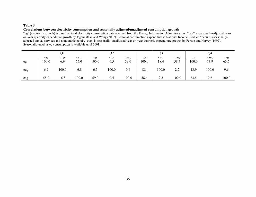
35
Table 3 Correlations between electricity consumption and seasonally adjusted/unadjusted consumption growth “eg” (electricity growth) is based on total electricity consumption data obtained from the Energy Information Administration. “cag” is seasonally-adjusted year-on-year quarterly expenditure growth by Jagannathan and Wang (2007). Personal consumption expenditure is National Income Product Account’s seasonally-adjusted annual services and nondurable goods. “cug” is seasonally-unadjusted year-on-year quarterly expenditure growth by Ferson and Harvey (1992). Seasonally-unadjusted consumption is available until 2001. Q1 Q2 Q3 Q4 eg cug cag eg cug cag eg cug cag eg cug cag eg 100.0 6.9 55.0 100.0 6.5 59.0 100.0 18.4 58.4 100.0 13.9 63.5 cug 6.9 100.0 -6.8 6.5 100.0 0.4 18.4 100.0 2.2 13.9 100.0 9.6 cag 55.0 -6.8 100.0 59.0 0.4 100.0 58.4 2.2 100.0 63.5 9.6 100.0

36
Table 4 The equity premium: Time-series evidence from the U.S. stock market (baseline) Electricity growth is December-to-December (Column 1) and annual (Column 2) total electricity consumption growth and is based on total electricity consumption data obtained from the Energy Information Administration (EIA). Garbage is the annual growth rate of municipal solid waste (MSW) provided by Environmental Protection Agency (EPA). Expenditure is annual growth rate of National Income Product Account’s seasonally-adjusted annual services and nondurable goods. P-J is the ultimate consumption growth by Parker and Julliard (2005). Q4-Q4 is the year-on-year fourth quarter expenditure growth by Jagannathan and Wang (2007). Dec-Dec is the year-on-year December (seasonally adjusted) expenditure growth. Following Campbell (1999) and Savov (2010), we use the beginning-of-period time convention when matching return data to all year-on-year growth rates computed using annual data. For instance, the calendar year return in year t will be matched to the garbage growth computed using annual garbage generation in year t and t+1. Panel A shows parameter estimates of CCAPM, Equation (1), for alternative measures of consumption risk. RRA is the relative risk aversion constant. Implied Rf is based on estimated RRA. Sample periods are from 1961 to 2008 except for garbage (1961-2007) and P-J (1961-2006). Panel B shows parameter estimates of CCAPM, Equation (1), for individual components of electricity consumption growth. Results in Panel B consider 1960–2002 data due to a change in the definition of each sector in 2003. Panel A. Alternative measures of consumption growth Electricity
(Dec-Dec) Electricity (annual)
Garbage Expenditure (annual)
Expenditure (Q4-Q4)
Expenditure (Dec-Dec)
P-J
RRA 17.3 19.9 17.5 42.7 40.8 32.4 83.1 RRA(s.e.) 3.7 11.9 8.5 23.8 25.1 18.2 - Implied Rf (%) 17.5 40.0 14.4 119.4 113.2 86.8 1190.5 Pricing error 0.0000 0.0000 0.0000 0.0000 0.0000 0.0000 1.6668 Panel B. Components of electricity consumption growth (Dec-Dec) Residential Commercial Industrial Res. & Com. Total RRA 12.4 31.5 12.7 17.0 16.5 RRA(s.e.) 3.2 9.9 3.9 4.3 3.9 Implied Rf (%) 11.4 122.5 -6.1 63.6 21.0 Pricing error 0.0000 0.0000 0.0000 0.0000 0.0000
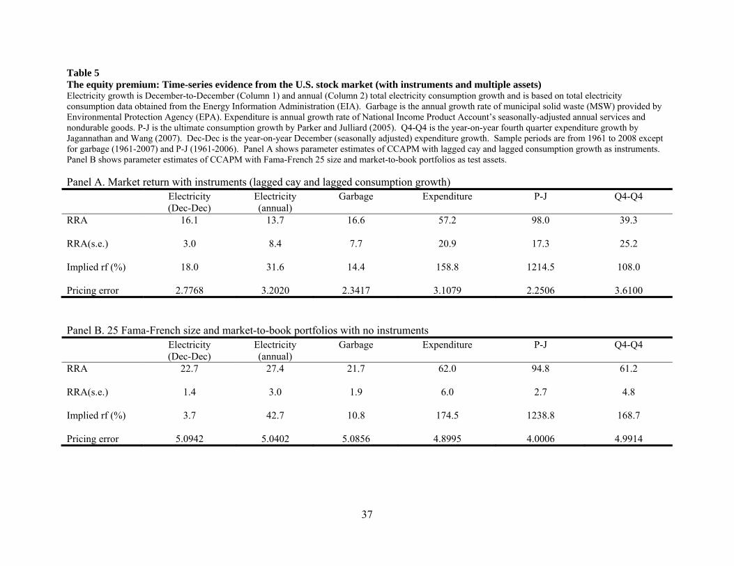
37
Table 5 The equity premium: Time-series evidence from the U.S. stock market (with instruments and multiple assets) Electricity growth is December-to-December (Column 1) and annual (Column 2) total electricity consumption growth and is based on total electricity consumption data obtained from the Energy Information Administration (EIA). Garbage is the annual growth rate of municipal solid waste (MSW) provided by Environmental Protection Agency (EPA). Expenditure is annual growth rate of National Income Product Account’s seasonally-adjusted annual services and nondurable goods. P-J is the ultimate consumption growth by Parker and Julliard (2005). Q4-Q4 is the year-on-year fourth quarter expenditure growth by Jagannathan and Wang (2007). Dec-Dec is the year-on-year December (seasonally adjusted) expenditure growth. Sample periods are from 1961 to 2008 except for garbage (1961-2007) and P-J (1961-2006). Panel A shows parameter estimates of CCAPM with lagged cay and lagged consumption growth as instruments. Panel B shows parameter estimates of CCAPM with Fama-French 25 size and market-to-book portfolios as test assets. Panel A. Market return with instruments (lagged cay and lagged consumption growth) Electricity
(Dec-Dec) Electricity (annual)
Garbage Expenditure P-J Q4-Q4
RRA 16.1 13.7 16.6 57.2 98.0 39.3 RRA(s.e.) 3.0 8.4 7.7 20.9 17.3 25.2 Implied rf (%) 18.0 31.6 14.4 158.8 1214.5 108.0 Pricing error 2.7768 3.2020 2.3417 3.1079 2.2506 3.6100 Panel B. 25 Fama-French size and market-to-book portfolios with no instruments Electricity
(Dec-Dec) Electricity (annual)
Garbage Expenditure P-J Q4-Q4
RRA 22.7 27.4 21.7 62.0 94.8 61.2 RRA(s.e.) 1.4 3.0 1.9 6.0 2.7 4.8 Implied rf (%) 3.7 42.7 10.8 174.5 1238.8 168.7 Pricing error 5.0942 5.0402 5.0856 4.8995 4.0006 4.9914
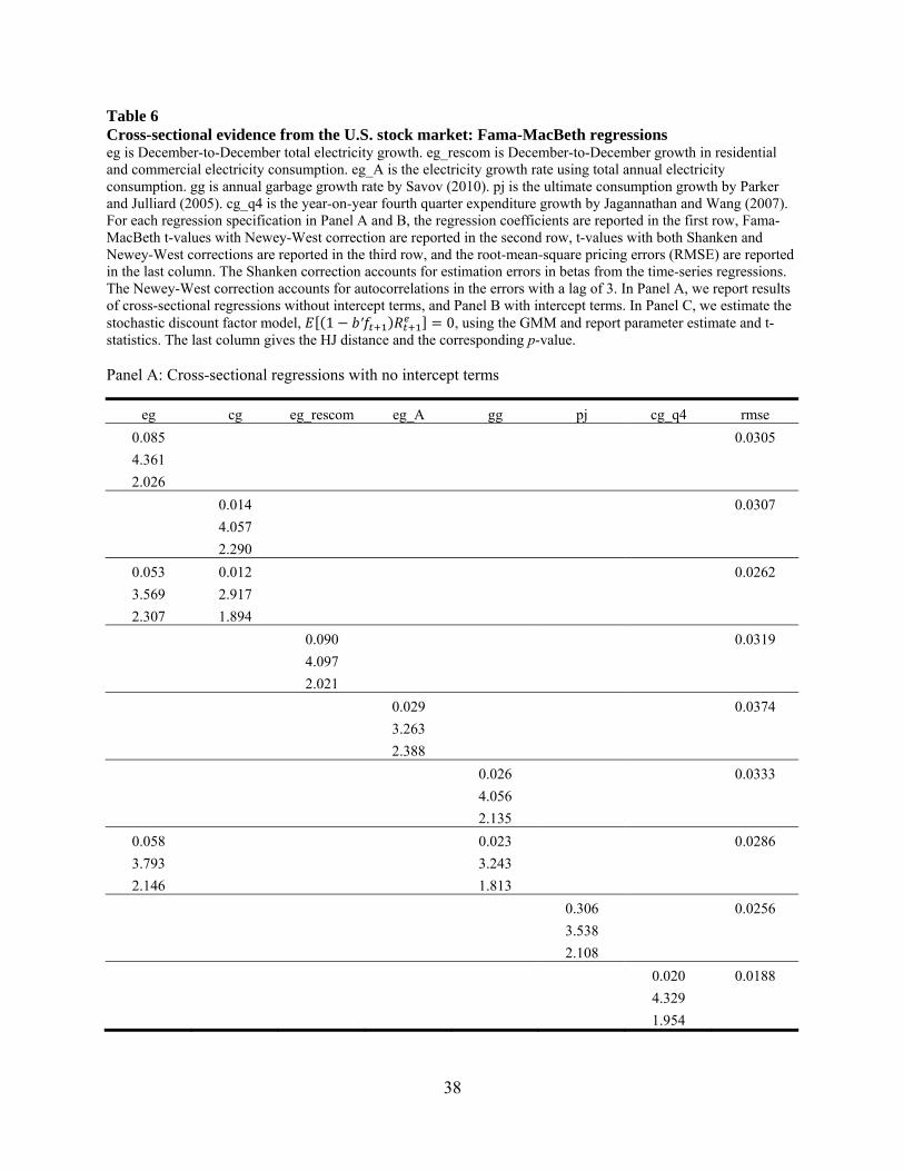
38
Table 6 Cross-sectional evidence from the U.S. stock market: Fama-MacBeth regressions eg is December-to-December total electricity growth. eg_rescom is December-to-December growth in residential and commercial electricity consumption. eg_A is the electricity growth rate using total annual electricity consumption. gg is annual garbage growth rate by Savov (2010). pj is the ultimate consumption growth by Parker and Julliard (2005). cg_q4 is the year-on-year fourth quarter expenditure growth by Jagannathan and Wang (2007). For each regression specification in Panel A and B, the regression coefficients are reported in the first row, Fama-MacBeth t-values with Newey-West correction are reported in the second row, t-values with both Shanken and Newey-West corrections are reported in the third row, and the root-mean-square pricing errors (RMSE) are reported in the last column. The Shanken correction accounts for estimation errors in betas from the time-series regressions. The Newey-West correction accounts for autocorrelations in the errors with a lag of 3. In Panel A, we report results of cross-sectional regressions without intercept terms, and Panel B with intercept terms. In Panel C, we estimate the stochastic discount factor model, 1 ′ 0, using the GMM and report parameter estimate and t-statistics. The last column gives the HJ distance and the corresponding p-value. Panel A: Cross-sectional regressions with no intercept terms
eg cg eg_rescom eg_A gg pj cg_q4 rmse 0.085 0.0305 4.361 2.026
0.014 0.0307 4.057 2.290
0.053 0.012 0.0262 3.569 2.917 2.307 1.894
0.090 0.0319 4.097 2.021
0.029 0.0374 3.263 2.388
0.026 0.0333 4.056 2.135
0.058 0.023 0.0286 3.793 3.243 2.146 1.813
0.306 0.0256 3.538 2.108
0.020 0.0188 4.329 1.954
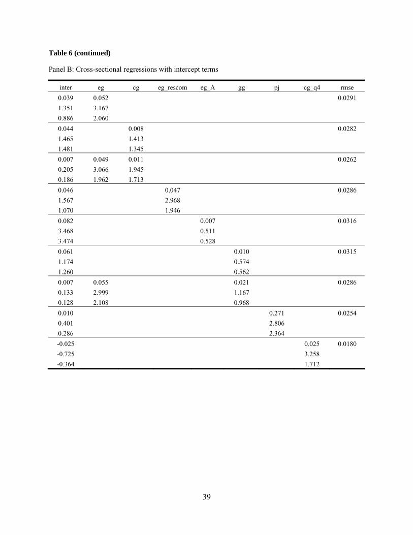
39
Table 6 (continued) Panel B: Cross-sectional regressions with intercept terms
inter eg cg eg_rescom eg_A gg pj cg_q4 rmse 0.039 0.052 0.0291 1.351 3.167 0.886 2.060 0.044 0.008 0.0282 1.465 1.413 1.481 1.345 0.007 0.049 0.011 0.0262 0.205 3.066 1.945 0.186 1.962 1.713 0.046 0.047 0.0286 1.567 2.968 1.070 1.946 0.082 0.007 0.0316 3.468 0.511 3.474 0.528 0.061 0.010 0.0315 1.174 0.574 1.260 0.562 0.007 0.055 0.021 0.0286 0.133 2.999 1.167 0.128 2.108 0.968 0.010 0.271 0.0254 0.401 2.806 0.286 2.364 -0.025 0.025 0.0180 -0.725 3.258 -0.364 1.712
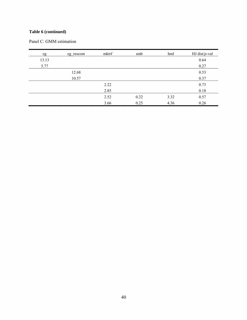
40
Table 6 (continued) Panel C: GMM estimation
eg eg_rescom mktrf smb hml HJ dist/p-val 13.13 0.64 5.77 0.27
12.68 0.53 10.57 0.37
2.22 0.73 2.85 0.18 2.52 0.22 3.32 0.57 3.66 0.25 4.36 0.26
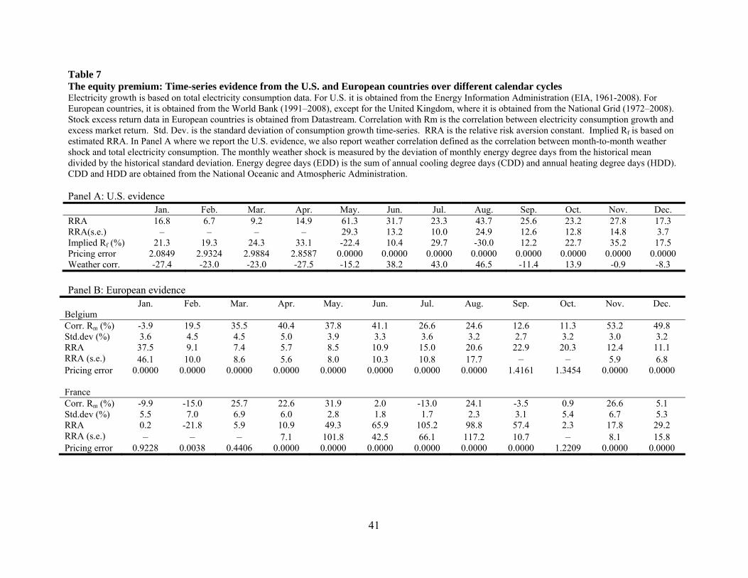
41
Table 7 The equity premium: Time-series evidence from the U.S. and European countries over different calendar cycles Electricity growth is based on total electricity consumption data. For U.S. it is obtained from the Energy Information Administration (EIA, 1961-2008). For European countries, it is obtained from the World Bank (1991–2008), except for the United Kingdom, where it is obtained from the National Grid (1972–2008). Stock excess return data in European countries is obtained from Datastream. Correlation with Rm is the correlation between electricity consumption growth and excess market return. Std. Dev. is the standard deviation of consumption growth time-series. RRA is the relative risk aversion constant. Implied Rf is based on estimated RRA. In Panel A where we report the U.S. evidence, we also report weather correlation defined as the correlation between month-to-month weather shock and total electricity consumption. The monthly weather shock is measured by the deviation of monthly energy degree days from the historical mean divided by the historical standard deviation. Energy degree days (EDD) is the sum of annual cooling degree days (CDD) and annual heating degree days (HDD). CDD and HDD are obtained from the National Oceanic and Atmospheric Administration. Panel A: U.S. evidence Jan. Feb. Mar. Apr. May. Jun. Jul. Aug. Sep. Oct. Nov. Dec. RRA 16.8 6.7 9.2 14.9 61.3 31.7 23.3 43.7 25.6 23.2 27.8 17.3 RRA(s.e.) – – – – 29.3 13.2 10.0 24.9 12.6 12.8 14.8 3.7 Implied Rf (%) 21.3 19.3 24.3 33.1 -22.4 10.4 29.7 -30.0 12.2 22.7 35.2 17.5 Pricing error 2.0849 2.9324 2.9884 2.8587 0.0000 0.0000 0.0000 0.0000 0.0000 0.0000 0.0000 0.0000 Weather corr. -27.4 -23.0 -23.0 -27.5 -15.2 38.2 43.0 46.5 -11.4 13.9 -0.9 -8.3 Panel B: European evidence
Jan. Feb. Mar. Apr. May. Jun. Jul. Aug. Sep. Oct. Nov. Dec. Belgium Corr. Rm (%) -3.9 19.5 35.5 40.4 37.8 41.1 26.6 24.6 12.6 11.3 53.2 49.8 Std.dev (%) 3.6 4.5 4.5 5.0 3.9 3.3 3.6 3.2 2.7 3.2 3.0 3.2 RRA 37.5 9.1 7.4 5.7 8.5 10.9 15.0 20.6 22.9 20.3 12.4 11.1 RRA (s.e.) 46.1 10.0 8.6 5.6 8.0 10.3 10.8 17.7 – – 5.9 6.8 Pricing error 0.0000 0.0000 0.0000 0.0000 0.0000 0.0000 0.0000 0.0000 1.4161 1.3454 0.0000 0.0000 France Corr. Rm (%) -9.9 -15.0 25.7 22.6 31.9 2.0 -13.0 24.1 -3.5 0.9 26.6 5.1 Std.dev (%) 5.5 7.0 6.9 6.0 2.8 1.8 1.7 2.3 3.1 5.4 6.7 5.3 RRA 0.2 -21.8 5.9 10.9 49.3 65.9 105.2 98.8 57.4 2.3 17.8 29.2 RRA (s.e.) – – – 7.1 101.8 42.5 66.1 117.2 10.7 – 8.1 15.8 Pricing error 0.9228 0.0038 0.4406 0.0000 0.0000 0.0000 0.0000 0.0000 0.0000 1.2209 0.0000 0.0000
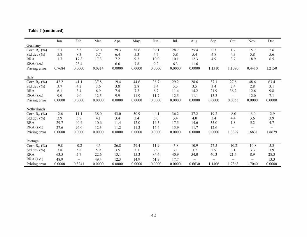
42
Table 7 (continued)
Jan. Feb. Mar. Apr. May. Jun. Jul. Aug. Sep. Oct. Nov. Dec. Germany Corr. Rm (%) 2.3 5.3 32.0 29.3 38.6 39.1 28.7 25.4 0.3 1.7 15.7 2.6 Std.dev (%) 5.8 8.3 5.7 6.4 5.3 4.7 5.8 5.4 4.8 4.3 5.8 5.6 RRA 1.7 17.8 17.3 7.2 9.2 10.0 10.1 12.3 4.9 3.7 18.9 6.5 RRA (s.e.) – 23.4 – 6.6 7.8 9.2 6.3 11.6 – – – – Pricing error 0.7684 0.0000 0.0314 0.0000 0.0000 0.0000 0.0000 0.0000 1.1310 1.1080 0.4410 1.2150 Italy Corr. Rm (%) 42.2 41.1 37.8 19.4 44.6 38.7 29.2 28.6 37.1 27.8 48.6 63.4 Std.dev (%) 3.7 4.2 3.6 3.8 2.8 3.4 3.3 3.5 3.4 2.4 2.8 3.1 RRA 6.1 3.4 6.9 7.4 7.2 6.7 11.4 14.2 21.9 36.2 12.6 9.8 RRA (s.e.) 9.9 9.0 12.5 9.9 11.9 11.7 12.5 11.1 13.3 – 12.0 7.1 Pricing error 0.0000 0.0000 0.0000 0.0000 0.0000 0.0000 0.0000 0.0000 0.0000 0.0355 0.0000 0.0000 Netherlands Corr. Rm (%) -2.6 11.1 38.0 43.0 50.9 44.1 36.2 37.2 19.2 -8.0 -6.0 -2.9 Std.dev (%) 3.9 3.9 4.1 3.4 3.4 3.0 3.4 4.0 3.4 4.4 3.6 3.9 RRA 29.7 40.4 10.6 11.4 12.0 16.3 17.5 14.6 35.0 1.8 5.2 4.7 RRA (s.e.) 27.6 96.0 12.3 11.2 11.2 15.4 15.9 11.7 12.6 – – – Pricing error 0.0000 0.0000 0.0000 0.0000 0.0000 0.0000 0.0000 0.0000 0.0000 1.3397 1.6831 1.8679 Portugal Corr. Rm (%) -9.8 -0.2 4.3 26.8 29.4 11.9 -3.8 10.9 27.5 -10.2 -10.8 5.3 Std.dev (%) 3.8 5.8 5.9 3.5 3.1 2.9 3.1 3.7 2.9 3.1 3.3 3.9 RRA 63.5 5.7 22.6 13.1 15.3 84.6 40.9 54.0 40.3 21.4 8.9 28.3 RRA (s.e.) 48.9 – 49.4 12.3 14.9 61.9 17.7 – – – – 13.3 Pricing error 0.0000 0.3241 0.0000 0.0000 0.0000 0.0000 0.0000 0.6630 1.1406 1.7363 1.7040 0.0000
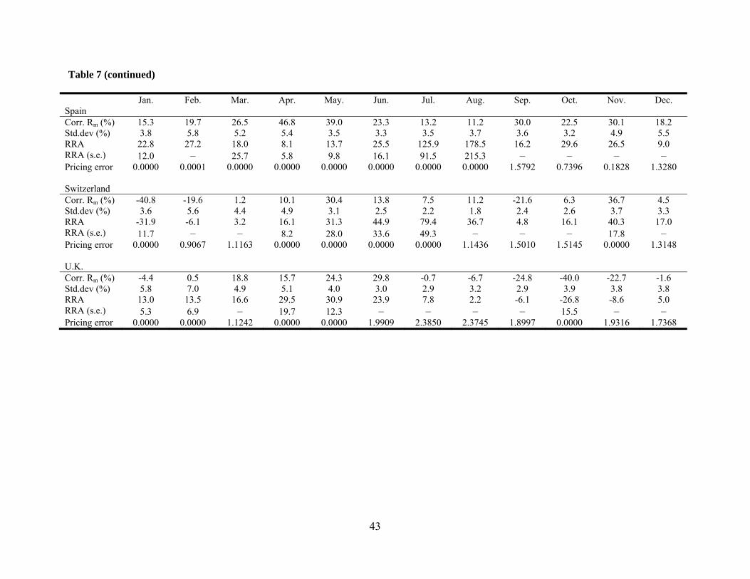
43
Table 7 (continued)
Jan. Feb. Mar. Apr. May. Jun. Jul. Aug. Sep. Oct. Nov. Dec. Spain Corr. Rm (%) 15.3 19.7 26.5 46.8 39.0 23.3 13.2 11.2 30.0 22.5 30.1 18.2 Std.dev (%) 3.8 5.8 5.2 5.4 3.5 3.3 3.5 3.7 3.6 3.2 4.9 5.5 RRA 22.8 27.2 18.0 8.1 13.7 25.5 125.9 178.5 16.2 29.6 26.5 9.0 RRA (s.e.) 12.0 – 25.7 5.8 9.8 16.1 91.5 215.3 – – – – Pricing error 0.0000 0.0001 0.0000 0.0000 0.0000 0.0000 0.0000 0.0000 1.5792 0.7396 0.1828 1.3280 Switzerland Corr. Rm (%) -40.8 -19.6 1.2 10.1 30.4 13.8 7.5 11.2 -21.6 6.3 36.7 4.5 Std.dev (%) 3.6 5.6 4.4 4.9 3.1 2.5 2.2 1.8 2.4 2.6 3.7 3.3 RRA -31.9 -6.1 3.2 16.1 31.3 44.9 79.4 36.7 4.8 16.1 40.3 17.0 RRA (s.e.) 11.7 – – 8.2 28.0 33.6 49.3 – – – 17.8 – Pricing error 0.0000 0.9067 1.1163 0.0000 0.0000 0.0000 0.0000 1.1436 1.5010 1.5145 0.0000 1.3148 U.K. Corr. Rm (%) -4.4 0.5 18.8 15.7 24.3 29.8 -0.7 -6.7 -24.8 -40.0 -22.7 -1.6 Std.dev (%) 5.8 7.0 4.9 5.1 4.0 3.0 2.9 3.2 2.9 3.9 3.8 3.8 RRA 13.0 13.5 16.6 29.5 30.9 23.9 7.8 2.2 -6.1 -26.8 -8.6 5.0 RRA (s.e.) 5.3 6.9 – 19.7 12.3 – – – – 15.5 – – Pricing error 0.0000 0.0000 1.1242 0.0000 0.0000 1.9909 2.3850 2.3745 1.8997 0.0000 1.9316 1.7368
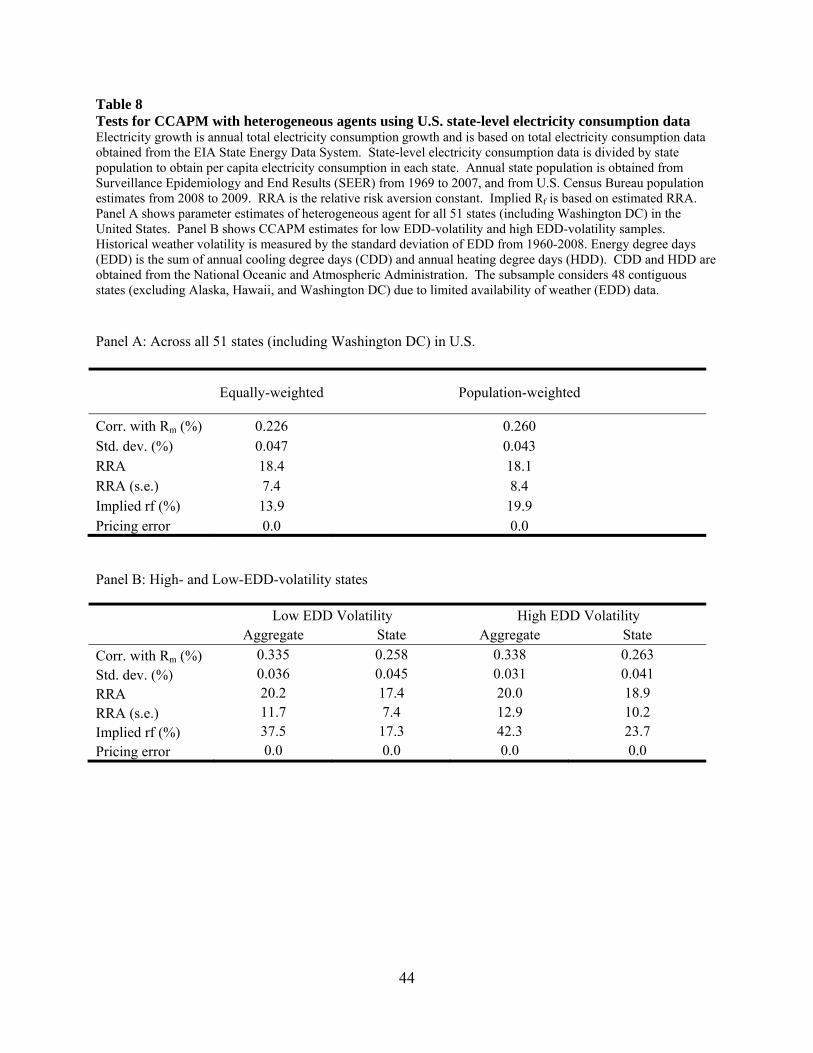
44
Table 8 Tests for CCAPM with heterogeneous agents using U.S. state-level electricity consumption data Electricity growth is annual total electricity consumption growth and is based on total electricity consumption data obtained from the EIA State Energy Data System. State-level electricity consumption data is divided by state population to obtain per capita electricity consumption in each state. Annual state population is obtained from Surveillance Epidemiology and End Results (SEER) from 1969 to 2007, and from U.S. Census Bureau population estimates from 2008 to 2009. RRA is the relative risk aversion constant. Implied Rf is based on estimated RRA. Panel A shows parameter estimates of heterogeneous agent for all 51 states (including Washington DC) in the United States. Panel B shows CCAPM estimates for low EDD-volatility and high EDD-volatility samples. Historical weather volatility is measured by the standard deviation of EDD from 1960-2008. Energy degree days (EDD) is the sum of annual cooling degree days (CDD) and annual heating degree days (HDD). CDD and HDD are obtained from the National Oceanic and Atmospheric Administration. The subsample considers 48 contiguous states (excluding Alaska, Hawaii, and Washington DC) due to limited availability of weather (EDD) data. Panel A: Across all 51 states (including Washington DC) in U.S.
Equally-weighted Population-weighted
Corr. with Rm (%) 0.226 0.260 Std. dev. (%) 0.047 0.043 RRA 18.4 18.1 RRA (s.e.) 7.4 8.4 Implied rf (%) 13.9 19.9 Pricing error 0.0 0.0 Panel B: High- and Low-EDD-volatility states Low EDD Volatility High EDD Volatility Aggregate State Aggregate State Corr. with Rm (%) 0.335 0.258 0.338 0.263 Std. dev. (%) 0.036 0.045 0.031 0.041 RRA 20.2 17.4 20.0 18.9 RRA (s.e.) 11.7 7.4 12.9 10.2 Implied rf (%) 37.5 17.3 42.3 23.7 Pricing error 0.0 0.0 0.0 0.0
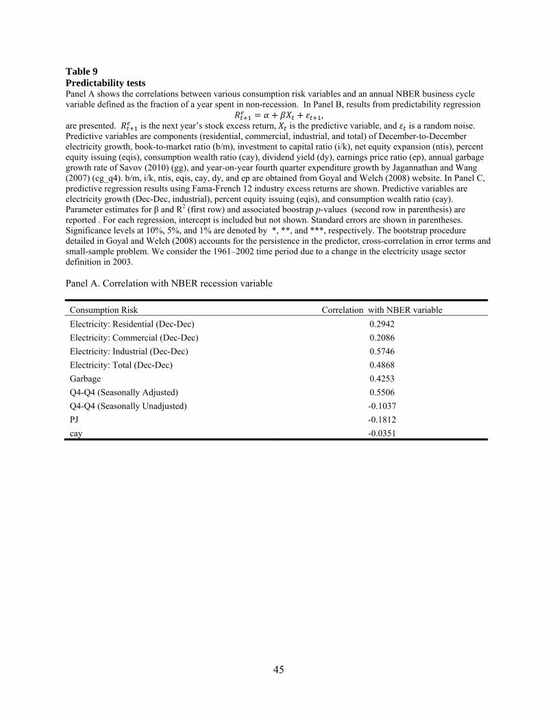
45
Table 9 Predictability tests Panel A shows the correlations between various consumption risk variables and an annual NBER business cycle variable defined as the fraction of a year spent in non-recession. In Panel B, results from predictability regression
, are presented. is the next year’s stock excess return, is the predictive variable, and is a random noise. Predictive variables are components (residential, commercial, industrial, and total) of December-to-December electricity growth, book-to-market ratio (b/m), investment to capital ratio (i/k), net equity expansion (ntis), percent equity issuing (eqis), consumption wealth ratio (cay), dividend yield (dy), earnings price ratio (ep), annual garbage growth rate of Savov (2010) (gg), and year-on-year fourth quarter expenditure growth by Jagannathan and Wang (2007) (cg_q4). b/m, i/k, ntis, eqis, cay, dy, and ep are obtained from Goyal and Welch (2008) website. In Panel C, predictive regression results using Fama-French 12 industry excess returns are shown. Predictive variables are electricity growth (Dec-Dec, industrial), percent equity issuing (eqis), and consumption wealth ratio (cay). Parameter estimates for β and R2 (first row) and associated boostrap p-values (second row in parenthesis) are reported . For each regression, intercept is included but not shown. Standard errors are shown in parentheses. Significance levels at 10%, 5%, and 1% are denoted by *, **, and ***, respectively. The bootstrap procedure detailed in Goyal and Welch (2008) accounts for the persistence in the predictor, cross-correlation in error terms and small-sample problem. We consider the 1961–2002 time period due to a change in the electricity usage sector definition in 2003. Panel A. Correlation with NBER recession variable
Consumption Risk Correlation with NBER variable Electricity: Residential (Dec-Dec) 0.2942 Electricity: Commercial (Dec-Dec) 0.2086 Electricity: Industrial (Dec-Dec) 0.5746 Electricity: Total (Dec-Dec) 0.4868 Garbage 0.4253 Q4-Q4 (Seasonally Adjusted) 0.5506 Q4-Q4 (Seasonally Unadjusted) -0.1037 PJ -0.1812 cay -0.0351

46
Table 9 (continued) Panel B. Predictability of Excess Market Returns
Prediction Variables Coefficient [p-value] Predictive Regression R2 [p-value] Electricity: Residential (Dec-Dec) -0.2509 0.0071
[0.298] [0.601] Electricity: Commercial (Dec-Dec) -0.7103 0.0195
[0.194] [0.372] Electricity: Industrial (Dec-Dec) -0.9102** 0.0968**
[0.026] [0.047] Electricity: Total (Dec-Dec) -0.9859* 0.0604
[0.059] [0.120] b/m 0.0649 0.0103
[0.609] [0.625] ik -9.2636 0.0315
[0.152] [0.260] ntis -1.8608 0.0311
[0.154] [0.271] eqis -0.6736** 0.1066**
[0.030] [0.034] cay 4.6631** 0.2282***
[0.016] [0.002] dy 0.0620 0.0212
[0.187] [0.364] ep 0.0784 0.0365
[0.266] [0.250] gg -0.8845 0.0232
[0.160] [0.342] cg_q4 -3.4692* 0.0717*
[0.055] [0.083]
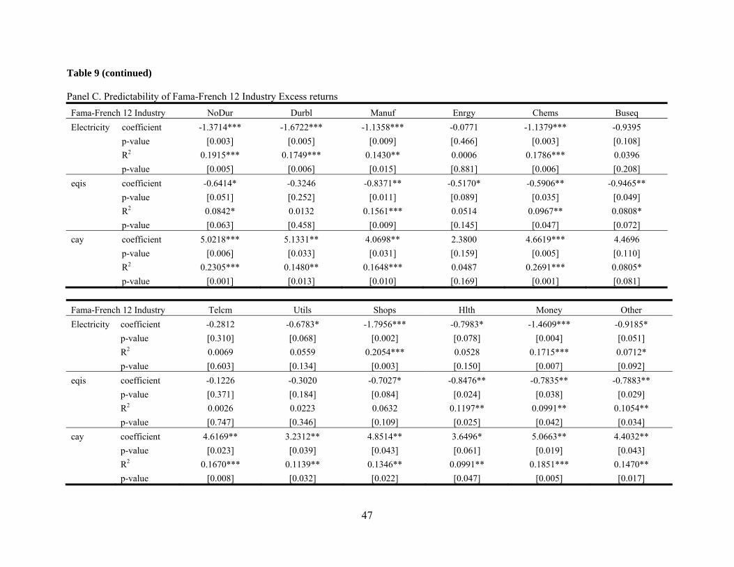
47
Table 9 (continued) Panel C. Predictability of Fama-French 12 Industry Excess returns Fama-French 12 Industry NoDur Durbl Manuf Enrgy Chems Buseq Electricity coefficient -1.3714*** -1.6722*** -1.1358*** -0.0771 -1.1379*** -0.9395
p-value [0.003] [0.005] [0.009] [0.466] [0.003] [0.108] R2 0.1915*** 0.1749*** 0.1430** 0.0006 0.1786*** 0.0396 p-value [0.005] [0.006] [0.015] [0.881] [0.006] [0.208]
eqis coefficient -0.6414* -0.3246 -0.8371** -0.5170* -0.5906** -0.9465** p-value [0.051] [0.252] [0.011] [0.089] [0.035] [0.049] R2 0.0842* 0.0132 0.1561*** 0.0514 0.0967** 0.0808* p-value [0.063] [0.458] [0.009] [0.145] [0.047] [0.072]
cay coefficient 5.0218*** 5.1331** 4.0698** 2.3800 4.6619*** 4.4696 p-value [0.006] [0.033] [0.031] [0.159] [0.005] [0.110] R2 0.2305*** 0.1480** 0.1648*** 0.0487 0.2691*** 0.0805* p-value [0.001] [0.013] [0.010] [0.169] [0.001] [0.081]
Fama-French 12 Industry Telcm Utils Shops Hlth Money Other Electricity coefficient -0.2812 -0.6783* -1.7956*** -0.7983* -1.4609*** -0.9185* p-value [0.310] [0.068] [0.002] [0.078] [0.004] [0.051] R2 0.0069 0.0559 0.2054*** 0.0528 0.1715*** 0.0712* p-value [0.603] [0.134] [0.003] [0.150] [0.007] [0.092] eqis coefficient -0.1226 -0.3020 -0.7027* -0.8476** -0.7835** -0.7883** p-value [0.371] [0.184] [0.084] [0.024] [0.038] [0.029] R2 0.0026 0.0223 0.0632 0.1197** 0.0991** 0.1054** p-value [0.747] [0.346] [0.109] [0.025] [0.042] [0.034] cay coefficient 4.6169** 3.2312** 4.8514** 3.6496* 5.0663** 4.4032** p-value [0.023] [0.039] [0.043] [0.061] [0.019] [0.043] R2 0.1670*** 0.1139** 0.1346** 0.0991** 0.1851*** 0.1470** p-value [0.008] [0.032] [0.022] [0.047] [0.005] [0.017]

48
Figure 1 Seasonality of electricity consumption Panel (a) shows monthly average electricity consumption for 1960-2008. Electricity consumption is based on electricity consumption obtained from the Energy Information Administration (EIA). For each sector, we normalize monthly electricity consumption by each year’s mean. Panel (b) shows monthly weather variation for 1960-2008. We measure the average monthly energy degree days (EDD) by the deviation of EDD from its historical mean each month, and then divide it by each month’s historical standard deviation. Energy Degree Days (EDD) is the sum of Cooling Degree Days (CDD) and Heating Degree Days (HDD). Historical CDD and HDD are obtained from the National Oceanographic and Atmospheric Administration (NOAA).
(a) Electricity consumption
(b) Historical Energy Degree Days (EDD)
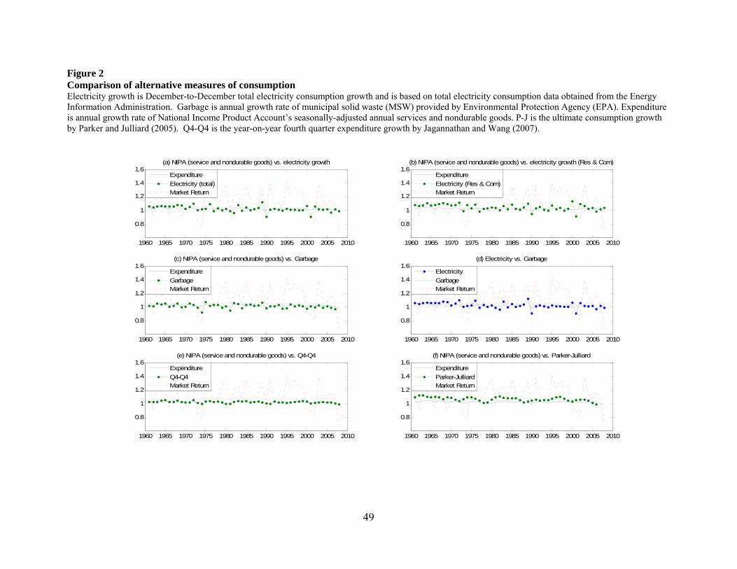
49
Figure 2 Comparison of alternative measures of consumption Electricity growth is December-to-December total electricity consumption growth and is based on total electricity consumption data obtained from the Energy Information Administration. Garbage is annual growth rate of municipal solid waste (MSW) provided by Environmental Protection Agency (EPA). Expenditure is annual growth rate of National Income Product Account’s seasonally-adjusted annual services and nondurable goods. P-J is the ultimate consumption growth by Parker and Julliard (2005). Q4-Q4 is the year-on-year fourth quarter expenditure growth by Jagannathan and Wang (2007).
1960 1965 1970 1975 1980 1985 1990 1995 2000 2005 2010
0.8
1
1.2
1.4
1.6(a) NIPA (service and nondurable goods) vs. electricity growth
ExpenditureElectricity (total)Market Return
1960 1965 1970 1975 1980 1985 1990 1995 2000 2005 2010
0.8
1
1.2
1.4
1.6(b) NIPA (service and nondurable goods) vs. electricity growth (Res & Com)
ExpenditureElectricity (Res & Com)Market Return
1960 1965 1970 1975 1980 1985 1990 1995 2000 2005 2010
0.8
1
1.2
1.4
1.6(c) NIPA (service and nondurable goods) vs. Garbage
ExpenditureGarbageMarket Return
1960 1965 1970 1975 1980 1985 1990 1995 2000 2005 2010
0.8
1
1.2
1.4
1.6(d) Electricity vs. Garbage
ElectricityGarbageMarket Return
1960 1965 1970 1975 1980 1985 1990 1995 2000 2005 2010
0.8
1
1.2
1.4
1.6(e) NIPA (service and nondurable goods) vs. Q4-Q4
ExpenditureQ4-Q4Market Return
1960 1965 1970 1975 1980 1985 1990 1995 2000 2005 2010
0.8
1
1.2
1.4
1.6(f) NIPA (service and nondurable goods) vs. Parker-Julliard
ExpenditureParker-JulliardMarket Return
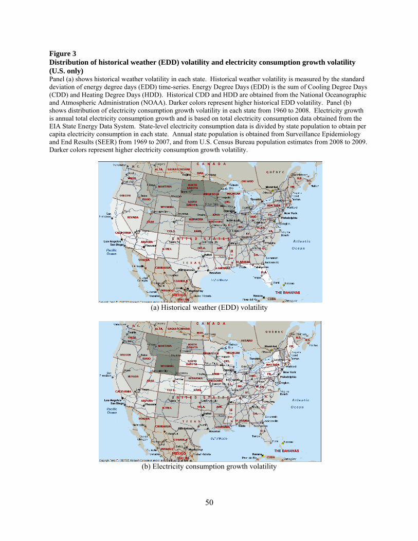
50
Figure 3 Distribution of historical weather (EDD) volatility and electricity consumption growth volatility (U.S. only) Panel (a) shows historical weather volatility in each state. Historical weather volatility is measured by the standard deviation of energy degree days (EDD) time-series. Energy Degree Days (EDD) is the sum of Cooling Degree Days (CDD) and Heating Degree Days (HDD). Historical CDD and HDD are obtained from the National Oceanographic and Atmospheric Administration (NOAA). Darker colors represent higher historical EDD volatility. Panel (b) shows distribution of electricity consumption growth volatility in each state from 1960 to 2008. Electricity growth is annual total electricity consumption growth and is based on total electricity consumption data obtained from the EIA State Energy Data System. State-level electricity consumption data is divided by state population to obtain per capita electricity consumption in each state. Annual state population is obtained from Surveillance Epidemiology and End Results (SEER) from 1969 to 2007, and from U.S. Census Bureau population estimates from 2008 to 2009. Darker colors represent higher electricity consumption growth volatility.
(a) Historical weather (EDD) volatility
(b) Electricity consumption growth volatility
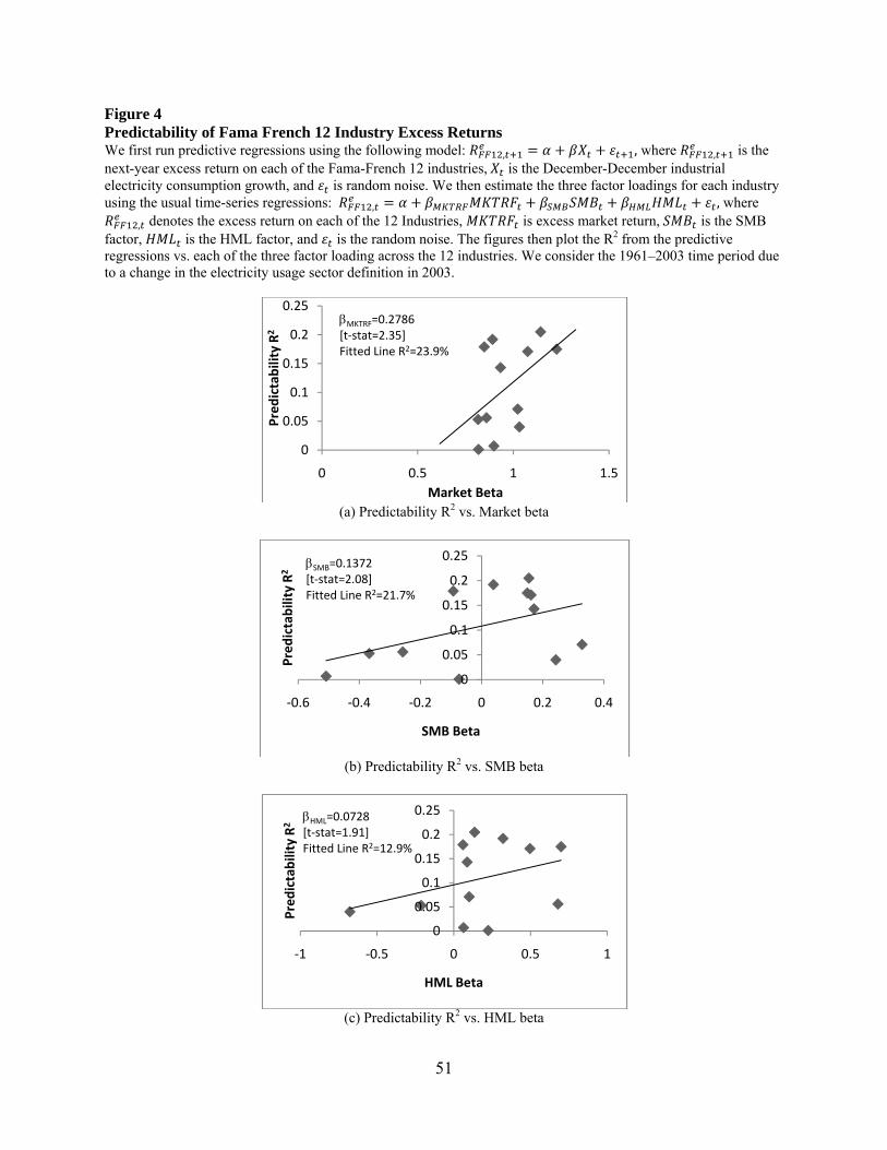
51
Figure 4 Predictability of Fama French 12 Industry Excess Returns We first run predictive regressions using the following model: , , where , is the next-year excess return on each of the Fama-French 12 industries, is the December-December industrial electricity consumption growth, and is random noise. We then estimate the three factor loadings for each industry using the usual time-series regressions: , , where
, denotes the excess return on each of the 12 Industries, is excess market return, is the SMB factor, is the HML factor, and is the random noise. The figures then plot the R2 from the predictive regressions vs. each of the three factor loading across the 12 industries. We consider the 1961–2003 time period due to a change in the electricity usage sector definition in 2003.
(a) Predictability R2 vs. Market beta
(b) Predictability R2 vs. SMB beta
(c) Predictability R2 vs. HML beta
0
0.05
0.1
0.15
0.2
0.25
0 0.5 1 1.5
Pred
ictability R2
Market Beta
βMKTRF=0.2786[t‐stat=2.35]Fitted Line R2=23.9%
0
0.05
0.1
0.15
0.2
0.25
‐0.6 ‐0.4 ‐0.2 0 0.2 0.4
Pred
ictability R2
SMB Beta
βSMB=0.1372[t‐stat=2.08]Fitted Line R2=21.7%
0
0.05
0.1
0.15
0.2
0.25
‐1 ‐0.5 0 0.5 1
Pred
ictability R2
HML Beta
βHML=0.0728[t‐stat=1.91]Fitted Line R2=12.9%