Hydrogeophysical Investigation of Groundwater Potential in Akamkpa Area

Cross River State Southern, Nigeria using Refraction Seismic and GPR

Method.Ndidiamaka Nchedo Eluwa1, Terhemba Theophilus Emberga2, Alexander Selemo3, John Chibuzor

Eluwa4 and George-Best Azuoko1.

1Department of Physics/Geology/Geophysics, Federal University Ndufu-Alike Ikwo2Department of Physics, Federal Polytechnic Nekede3Department of Geology, Federal University of Technology, Owerri4Agrometerological Unit, National Root and Crop Research Institute, Umudike

E-mail: ndidiamakaeluwa@gmail.com

ABSTRACT

Refraction seismic and GPR survey were carried out in Akamkpa area, Cross River State within

latitude 50000N to 5048'N and longitude 8012'E to 9000'E to delineate aquiferous zones so that

productive boreholes can be drilled. The study area is part of Oban Massif Basement complex

which is overlain by the cretaceous-tertiary sediment of Calabar Flank. The metamorphic rock

units in the area are: Phylites, Schists, Gneisses and Amphibolites. These rocks are intruded by

pegmatites, granites, granodorite, diorite, and dolerite. The refraction seismic survey was done in

three(3) traverses with length up to 1km. From the results, it was observed that the velocities for

the first layer in the three (3) traverses varied from 300m/s-380m/s with depth between 0.5m to

1.8m, this indicated the weathered layer top soil. The second layer velocities varied from

624m/s-746m/s with depth between 1.8m-9.8m, lateritic rocks were observed, the third layer

velocities varied from 1058m/s to 1204m/s with depth between 5.8m-18.2m, with sand/sandstone

observed. The last layer was made up of granite with velocity up to 1805m/s at depth of 18.2m

below. Only four geologic layers were observed. From the GPR survey, profile 1 and 2 showed

four distinct geologic layers with average velocities of 8cm/ns, 8cm/ns, 12cm/ns and 16cm/ns

respectively and electrical conductivity of 7.75Ωm-1, 16.2 Ωm-1, 26.5Ωm-1 and 35.5 Ωm-1

respectively. Profile 3 indicated three geologic layers with velocities 3cm/ns, 7cm/ns and

13cm/ns respectively. From the study, productive boreholes with good drinking water is

expected to be within 30m-50m (100ft-165ft) depth.

INTRODUCTION

Akamkpa area is part of Oban Massif basement complex, southern Nigeria. The

inhabitants of this area reside in scattered hamlets, villages, and small towns. They

are mostly farmers; water demand in the area is mainly for domestic and agricultural

uses. Majority of the people depend on shallow dug wells and streams which are

mostly seasonal. The streams are also generally remote, polluted and hazardous. Most

of the natural resources in the Cross River State occur in Akamkpa area (Arong,

2013). Presently, there exists oil palm and rubber plantations, quarries and holiday

resorts. There is also a game reserve manage by the World Wildlife Fund (WWF) and

funded by the United Nations in the area. These existing facilities and the need to

provide portable water to rural dwellers, therefore, prompted the quest to develop

water resources within the area. The works aimed at using a combination of

refraction seismic and radar imageries in Akamkpa to delineate aquiferous zones so

that productive boreholes can be drilled within the area.

GEOLOGY OF THE STUDY AREA

Akamkpa area is part of the Precambrian Oban Massif, which is overlain by

cretaceous-Tertiary sediments of the Calabar Flank. The metamorphic rock units in

this area are: phylites, schists, gneisses, and amphibolites. These rocks are intruded

by pegmatites, granites, granodiorites, diorites, tonalites, Monzonites, and dolerites

(Ekwueme, 1990). Associated with the rocks are charnokites which occur as

enclaves in gneisses and granodiorites (Fig. 1)

Fig1 : Geologic map of Oban Massif

These rocks record three phase of tectonothermal events which have affected the

Nigerian basement with the most resent being the Pan-African Orogeny dating

about 600±150 Ma ago. The main results of the deformation include fractures,

faults, folds, and dykes trending N-S, NE-SW, and NW-SE directions. Similar

trends characterized major lineaments revealed by remote sensing and

aeromagnetic interpretation (Arong and Oghenero, 2013).

METHODOLOGY

The geophones were laid 2m apart and were connected to geophone cable; a trigger

was connected to a 2kg hammer. The geophone cable was then connected to a

seismogram. When the hammer hits the metal plate, the geophones will give out

seismic waves, the seismograph records the signals received from the geophones

and were displayed on a computer. The group geophones were used to filter noise,

battery was used to power the seismogram. P-waves were generated. Forward and

reverse shooting were done. The penetration was not too deep, since hammer

shooting was used instead of dynamites. At each shot point the arrival times for

each of the geophone were recorded. For the GPR survey, an electromagnetic

micro pulse was emitted into the earth by a transmitting antenna. The

electromagnetic wave propagated into the subsurface and reflected from boundary

layers or buried objects (targets) of variable density. The reflected waves were

detected by the receiving antenna, amplified and processed. The amplified waves

were digitally recorded by the digital recorder. GPR measurements were done in

three profiles; the measurements were recorded by maintaining a fixed distance

between the transmitting antennas and receiving antenna along the survey

measurement line. The GPR survey grid was established in each entry area with

survey line trending N-E direction. Three survey lines were established each

approximately 1000m (1km) long and spaced 1m apart.

Software was used on the GPR data processing to show the amplitude maps and

rock types. The recommended processing stages were employed; which includes

range gain, band-pass filtering, frequency filtering, spectral whitening, background

removal, migration, Hilbert transformation, deconvolution, smoothing, stacking,

and finally, re-sampling of processed digital data to produce the final images

(Conyers, 2011, 2012, 2013).

The usual final product of GPR mapping involves the presentation of amplitude

images that are the product of a computer analysis of thousands of reflection

“anomalies”(Annan, 2009).

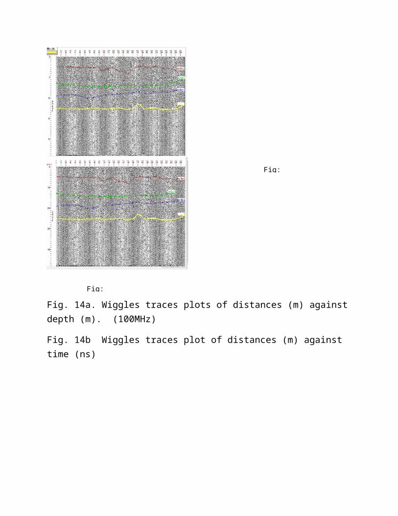
In the GPR method, individual wiggle trace (as seen in Fig 14a &b, 15a&b and

16a&c) are used to produce reflection profiles, which are then re-sampled to

generate amplitude slice map (Fig. 14d,15e and 16b). Each of these processing

steps produces important images that must be understood, integrated and analyzed

in conjunction during interpretation. The nature of the ground and geological

features were defined and understood.

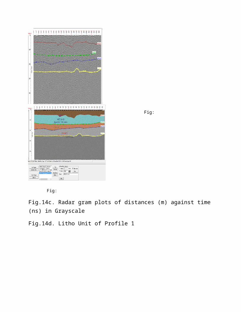
The wiggle traces and profile were used to delineate the lithological units as seen

in Fig.14d, 15e and 16b that is the radargram plots. The wiggle traces shows the

amplitude reflections of the different layers. (Conyers and Dean, 1997)

Wiggle traces/profiles in amplitude slicing methods were used to generate

anomalies at vary depths from one horizon within different slices in the ground.

RESULTS

Seismic Refraction

Seismic velocity information was correlated with rock type and used in identifying

subsurface materials. Due to overlapping of velocities for different rocks, the

identification of rock type was exclusively on velocity. It can however be used in a

small area where range of velocity is small and therefore certain rocks can be

identified based on velocity.

The processing of the data is often based on the first arrivals, since it permits

accurate interpretation and easy recording of their travel times. The Wyrobek

method (Telford et al, 1976) was used to analyze the data in this study. This uses

graphic aids to facilitate the routine computations. Based on the Wyrobek’s

approach (Burke, 1970) a plot of the travel time (T) versus the detector position of

all the receiving stations along each traverse was obtained.

The slope of these graphs were used to obtain the average velocities V1, V2, V3, etc. for

both the first layer and the refractors. The intercept time was also determined from the

graph. To obtain the depth to refractor at each shot point, the intercept time is divided by

two to give the half – intercept time often called the delay time D. Values of the delay

time D at each shot point is thus multiplied by an appropriate factor F to obtain the depth.

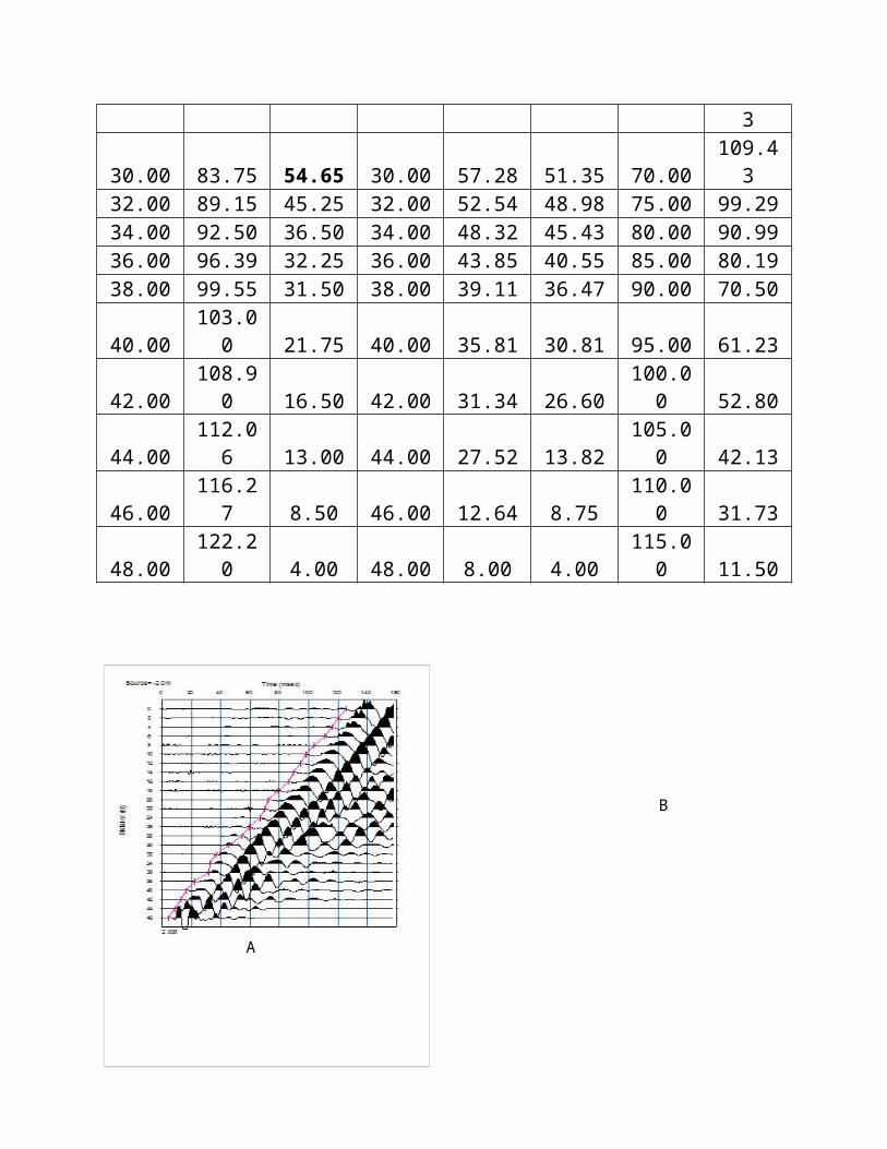
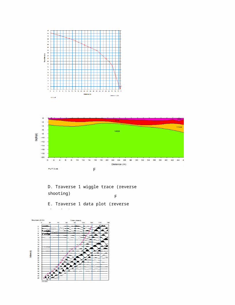
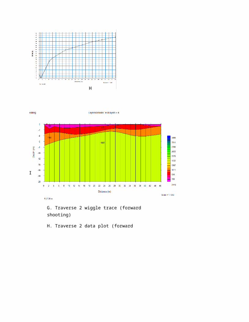
TRAVERSE: 1 2 3

X(M) T(ms)F T(ms)R X(M) T (ms)F T (ms)R X(M) T(ms)F2.00 5.00 125.75 2.00 124.31 118.91 0.00 220.834.00 11.72 120.50 4.00 119.57 116.25 5.00 217.286.00 17.64 116.25 6.00 117.00 113.75 10.00 216.368.00 26.07 111.00 8.00 110.50 111.53 15.00 212.8010.00 38.84 103.75 10.00 105.87 105.87 20.00 211.3512.00 43.85 98.50 12.00 101.92 103.50 25.00 205.3014.00 48.98 94.55 14.00 97.75 100.21 30.00 192.7916.00 53.46 89.41 16.00 91.25 95.73 35.00 188.3118.00 56.75 86.51 18.00 86.51 91.91 40.00 175.5320.00 60.57 79.01 20.00 82.04 82.30 45.00 170.2522.00 65.71 72.50 22.00 74.53 72.55 50.00 151.7024.00 69.26 69.75 24.00 72.16 67.16 55.00 138.9326.00 71.90 67.00 26.00 68.87 61.49 60.00 127.3428.00 76.11 59.65 28.00 60.57 57.54 65.00 119.8330.00 83.75 54.65 30.00 57.28 51.35 70.00 109.4332.00 89.15 45.25 32.00 52.54 48.98 75.00 99.2934.00 92.50 36.50 34.00 48.32 45.43 80.00 90.9936.00 96.39 32.25 36.00 43.85 40.55 85.00 80.1938.00 99.55 31.50 38.00 39.11 36.47 90.00 70.5040.00 103.00 21.75 40.00 35.81 30.81 95.00 61.2342.00 108.90 16.50 42.00 31.34 26.60 100.00 52.8044.00 112.06 13.00 44.00 27.52 13.82 105.00 42.1346.00 116.27 8.50 46.00 12.64 8.75 110.00 31.7348.00 122.20 4.00 48.00 8.00 4.00 115.00 11.50

B

A

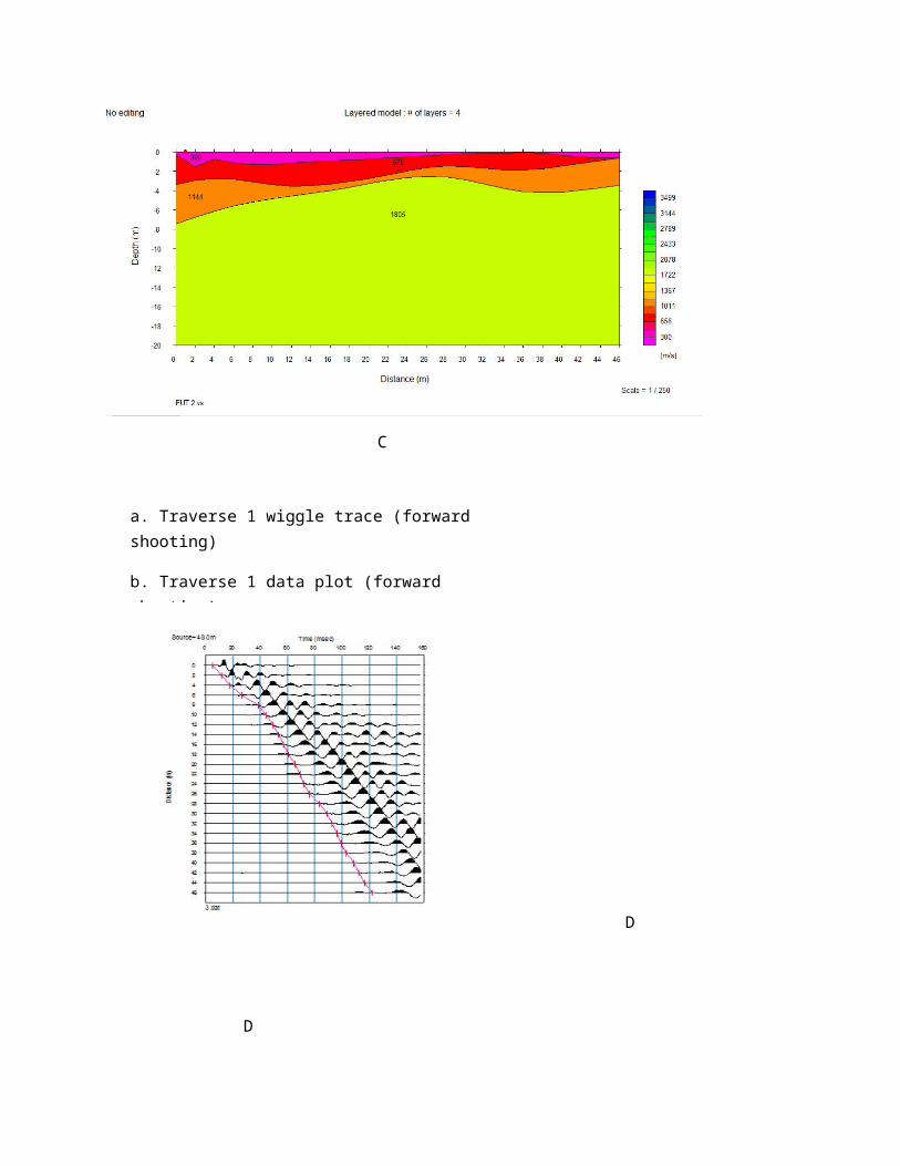
a. Traverse 1 wiggle trace (forward shooting)

b. Traverse 1 data plot (forward shooting)

c. Traverse1 layer model (forward shooting)

C

D

D

F

D. Traverse 1 wiggle trace (reverse shooting)

E. Traverse 1 data plot (reverse shooting)

F. Traverse1 layer model (reverse shooting)

F

H

I

G. Traverse 2 wiggle trace (forward shooting)

H. Traverse 2 data plot (forward shooting)

I. Traverse2 layer model (forward shooting)

JK

L

J. Traverse 2 wiggle trace (reverse shooting)

K. Traverse 2 data plot (reverse shooting)

L. Traverse2 layer model (reverse shooting)

NM

O

L

The main objectives and end product of any seismic work is the ability to interpret

seismic data in geological terms (Dobrin, 1960). In most seismic refraction

techniques, the assumption lies on the value of the velocity (V1) of the section

above the refractor. This is because of the heterogenous composition of the

superficial deposit which make the overburden velocity rarely constant, (Dobrin,

1976, Bruce, 1973).

However, in this interpretation, by combining the general geology of the area and

using standard tables that provides approximate range of velocities of longitudinal

seismic waves through some earth materials. A good attempt is made to obtain a

reasonable geological structure for the surveyed area.

The time-distance graph was plotted (using Excel package), Fig; B, E, H, K and N

were samples of the resulting time-distance graph plotted with data from Fig; A, D,

G, J and M. The graphs showed a four layer case as seen in Fig; C, F, I, L and O

The slopes of the layers were calculated and the inverse of the slopes gave the

values for the velocities, the depths to refractors were also calculated using

software (IXRefraX and Seisimager).

Based on the values of the velocities obtained, the first layer velocity throughout

the entire survey varies between 300m/s – 380m/s with depth between 0.5m –

1.8m. It was observed that the first layer is composed of weathered basement top

soil. The second layer velocity varies from 624m/s – 746m/s and was used to

M. Traverse 3 wiggle trace (forward shooting)

N. Traverse 3 data plot (forward shooting)

O. Traverse3 layer model (forward shooting)

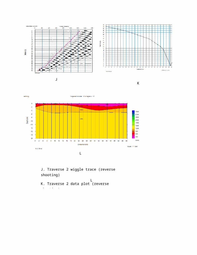
obtain the contour map for V2 as seen in fig. C, F, I, L and O. The velocities were

increasing with depth. The characteristics of lateritic rocks were observed at the

depth between 1.8m - 9.8m. The velocity values of the third layer vary from

1058m/s – 1204m/s with depth between 5.8m -18.2m. The characteristics of sand

and sandstone were observed. The last layer was made up of granite with velocity

up to 1805m/s at the depth of 18.2 below. Only four geologic layers were observed

throughout the study area.

GPR Survey Result

Each depth that is sliced contains only a portion of the horizon’s reflection which

appears as individual “anomalies” that are present at discrete depths as seen in Fig.

14d, 15e and 16b.

From profile 1 and 2; it was observed that the study area were made up of four

layers, the top soil, wet sand, dry sand/sandstone and granites respectively with the

following velocities; 13cm/ns, 9cm/ns, 6cm/ns and 19cm/ns and electrical

conductivity of 5.3Ωm-1, 11.1 Ωm-1, 25 Ωm-1 and 25 Ωm-1 respectively in profile 1.

Profile 2, the following velocities were observed; 3cm/ns, 7cm/ns,18cm/ns and

14cm/ns respectively and the electrical conductivity of 10.2 Ωm-1, 21.3 Ωm-1, 28

Ωm-1 and 46 Ωm-1 respectively.

Profile 3, it was observed that the profile has only three layers namely; wet

sand/sandstone, dry sand/ sandstone and granites respectively, with the following

velocities 3cm/ns, 7cm/ns and 13cm/ns and the electrical conductivity of 10.6 Ωm -

1, 5.2 Ωm-1 and 21 Ωm-1 respectively.

Fig. 14a. Wiggles traces plots of distances (m) against depth (m). (100MHz)

Fig. 14b Wiggles traces plot of distances (m) against time (ns)

Fig.14c. Radar gram plots of distances (m) against time (ns) in Grayscale

Fig.14d. Litho Unit of Profile 1

Fig: 14c Fig: 14d

Fig: 14aFig: 14b

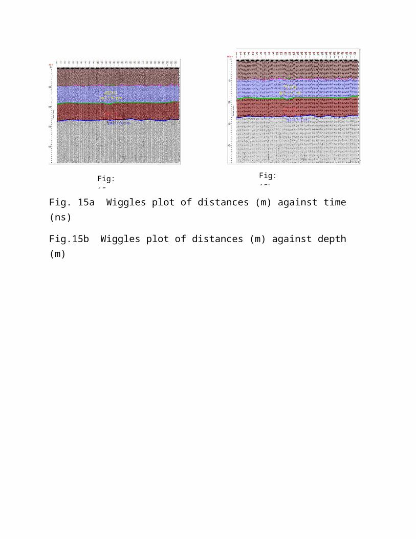
Fig. 15a Wiggles plot of distances (m) against time (ns)

Fig.15b Wiggles plot of distances (m) against depth (m)

Fig. 15c Radargram plot of distance(m) against depth (m) (100MHz)

Fig. 15d Radargram plot of distances (m) against time (ns)

Fig: 15c Fig: 15d

Fig: 15a Fig: 15b

Fig. 15e Litho Unit of Profile 11

Fig.16a Wiggles trace plot of distances (m) against time (ns) .

Fig.16b Litho Unit of Profile 111

Fig: 16a Fig: 16b

Fig. 16c Radargram plot of distances (m) against depth (m) in colour scale.

Fig. 16d Radargram plot of distances (m) against time (ns) in grayscale.

Fig. 16e Radargram plot of distances (m) against depth (m) in grayscale.

Conclusions

Refraction seismic and GPR methods have been employed in the study of the

hydrogeology of Akamkpa area. From the ongoing study, it has been seen that

Fig: 16cFig: 16d

refraction seismograph is used for shallow subsurface investigation. GPR and

refraction seismic have similar principles except that GPR uses electromagnetic

energy while seismic method uses acoustic energy.

After careful interpretation of the data, the area showed a geologic setting of three

to four geologic layers. However, the four layers case is more abundant in the area.

The thickness of the layers varies from place to place due to differences in

elevation, rock type and weathering characteristics.

Though interpretation of refraction seismic show that the study area is made up of

predominantly four layers while that of GPR show that traverse 1 and 2 are made

up of four layers while traverse 3 showed three layers.

These layers are; overburden composed of lateritic and weathered basement, the

second layer is made up of wet sand, whereas the third layer is made up of dry

sand/sandstone and the fourth layer is made up of granite. The thickness of first

layer is about 0.5m to 1.8m with average thickness of 1.15m. The thickness of the

second layer varies from 1.8m to 9.8m with average thickness of 5.8m. The

thickness of the third layer also varies from 5.8m to 18.2m with average thickness

of 12m and the last layer is a depth > 50m.

The depth to water table has also been seen to vary from place to place. Depth to

water is between 18.5m to 50m (61ft to 165ft).

Recommendations

It is recommended that lower GPR frequencies should be employed during GPR

survey in order to increase the rate of depth of penetration because in high GPR

frequencies, the penetration depth decreases. The rock types observed in the study

area are highly resistive. The study area is a good site for borehole drilling.

References

Annan P. 2009. Electromagnetic principles of ground penetrating radar. In: Ground Penetrating Radar: Theory and Applications, (ed. H.M. Jol), pp. 3–40. Elsevier, New York.

Arong, T.O. and Oghenero, A.E. 2013; Evaluation of Groundwater Resource in Akamkpa Area, CRS Nigeria. Advances in Applied Science Research, 4(5); 10-24.

Borchert, O.,2008; Receiver Design for a Directional Borehole Radar System Dissertation, University of Wuppertal.

Burke, K. B. S. 1970, "A Review of Some Problems of Seismic Prospecting for Groundwater in Surficial Deposits," in Mining and Groundwater Geophysics, 1967, Geological Survey of Canada, Economic Report No. 26, Ottawa. Canada.

Bruce , B.R., 1973; seismic refraction exploration for engineering site investigations. Explosive Excavation Research Laboratory Livermore, California

Cassidy N.J. 2009. Electrical and magnetic properties of rocks, soil and fluids. In: Ground Penetrating Radar: Theory and Applications, (ed. H.M. Jol), pp. 41–72. Elsevier, New York.

Conyers L.B. 2011. Ground-penetrating radar mapping of non-reflective archaeological features. In: Proceedings of the 9th International Conference on Archaeological Prospection, September 19–24, Izmir,

Conyers, L.B. 2012. Interpreting Ground-penetrating Radar for Archaeology. Left Coast Press, Walnut Creek, California.

Conyers L.B. 2013. Ground-penetrating Radar for Archaeology, 3rd ed. Rowman and Littlefield Publishers, Alta Mira Press, Latham, Maryland.

Conyers L.B. and Leckebusch J. 2010. Geophysical archaeology research agendas for the future: Some ground-penetrating radar examples. Archaeological Prospection 17, 117–123.

Conyers, L. B. and Dean, G. 1997; Ground Penetrating Radar: An Introduction for Archaeologists. Walnut Creek, CA.: Altamira Press.

Cornick, M., Koechling, J., Stanley, B. and Zhang, B. (2016). Localizing Ground Penetrating RADAR: A Step Toward Robust Autonomous Ground Vehicle

Localization". Journal of Field Robotics 33 (1): 82–102. doi:10.1002/rob.21605. ISSN 1556-4967.

Damiata B.N., Sternberg J.M., Bolender D.J. and Zoëga G. 2013. Imaging skeletal remains with ground-penetrating radar: comparative results over two graves from Viking Age and Medieval churchyards on the Stóra-Seyla farm, northern Iceland. Journal of Archaeological Science 40, 268–278.

Daniels, D.J, (2004). Ground Penetrating Radar (2nd edition.). Knoval (Institution of Engineering and Technology). pp. 1–4. ISBN 978-0-86341-360-5.

Daniels J.J., Wielopolski L., Radzevicius S. and Bookshar J. 2003. 3D GPR polarization analysis for imaging complex objects. Symposium on the Application of Geophysics to Engineering and Environmental Problems Proceedings, pp. 585–597.

Dobrin, M. B. 1960; Introduction to Geophysical Prospecting. McGraw-Hill, New York.

Ekwueme, B.N. 1990; Precambrian Res, 47:271-286

ETSI EG 202 730 V1.1.1 (2009–09), "Electromagnetic compatibility and Radio spectrum Matters (ERM); Code of Practice in respect of the control, use and application of Ground Probing Radar (GPR) and Wall Probing Radar (WPR) systems and equipment, An impulse generator for the ground penetrating radar

"Gems and Technology - Vision Underground". 2014; The Ganoksin Project. Retrieved 5 February 2014.

"History of Ground Penetrating Radar Technology". Ingenieurbüro obonic. Retrieved 13 February 2016.

Hofinghoff, Jan-Florian (2013). "Resistive Loaded Antenna for Ground Penetrating Radar Inside a Bottom Hole Assembly". IEEE Transactions on Antennas and Propagation (IEEE) 61(12). doi:10.1109/TAP.2013.2283604.

Ivashov, S. I.; Razevig, V. V.; Vasiliev, I. A.; Zhuravlev, A. V.; Bechtel, T. D.; Capineri, L. (2011). "Holographic Subsurface Radar of RASCAN Type: Development and Application" (PDF).IEEE Journal of Selected Topics in Applied Earth Observation and Remote Sensing 4 (4): 763–778. doi:10.1109/JSTARS.2011.2161755. Retrieved 26 September 2013.

Linford N. 2014. Rapid processing of GPR time slices for data visualisa-tion during field acquisition. In: Proceedings of the 15th International Conference on Ground Penetrating Radar (eds S. Lambot, A. Giannopoulos, L. Pajewski, F. André, E. Slob and C. Craeye), pp. 731–735. Square Brussels Meeting Centre, Brussels, Belgium: Université Catholique de Louvain.

Masini,N, Persico, R. Rizzo, E. (2005). Some examples of GPR prospecting for monitoring of the monumental heritage. Journal of Geophysics and Engineering 7 (2), 190, doi:10.1088/1742-2132/7/2/S05

Novo A., Grasmueck M., Viggiano D.A. and Lorenzo H. 2008. 3D GPR in archaeology: what can be gained from dense data acquisition and processing? In: Proceedings of the 12th International Conference on Ground Penetrating Radar (GPR 2008), Birmingham, pp. 16–19.

Sala J. and Linford N. 2012. Processing stepped frequency continuous wave GPR systems to obtain maximum value from archaeological data sets. Near Surface Geophysics 10(1), 310.

Trinks I., Johansson B., Gustafsson J., Milsson J., Friborg J., Gustafsson J.N. , 2010. Efficient, large-scale archaeological prospection using a true three-dimensional ground-penetrating radar array system. Archaeological Prospection 17, 175–186.

Wilson, M. G. C., Henry, G. and Marshall, T. R. (2006). "A review of the alluvial diamond industry and the gravels of the North West Province, South Africa" (PDF). South African Journal of Geology (Geological Society of South Africa) 109 (3): 301–314. doi:10.2113/gssajg.109.3.301. Retrieved 9 December 2012.

Zhuravlev, A.V.; Ivashov, S.I.; Razevig, V.V.; Vasiliev, I.A.; Türk, A.S.; Kizilay, A. (2013). "Holographic subsurface imaging radar for applications in civil engineering". (PDF). IET International Radar Conference. Xi'an, China: IET. doi:10.1049/cp.2013.0111 http://www.rslab.ru/downloads/A0065.pdf.