Eindhoven University of Technology

MASTER

Seawater desalination and windenergy : a system analysis

Feron, Paul

Award date:1984

Link to publication

DisclaimerThis document contains a student thesis (bachelor's or master's), as authored by a student at Eindhoven University of Technology. Studenttheses are made available in the TU/e repository upon obtaining the required degree. The grade received is not published on the documentas presented in the repository. The required complexity or quality of research of student theses may vary by program, and the requiredminimum study period may vary in duration.

General rightsCopyright and moral rights for the publications made accessible in the public portal are retained by the authors and/or other copyright ownersand it is a condition of accessing publications that users recognise and abide by the legal requirements associated with these rights.

• Users may download and print one copy of any publication from the public portal for the purpose of private study or research. • You may not further distribute the material or use it for any profit-making activity or commercial gain

TECHNISCHE HOGESCHOOL EINDHOVEN

Afdeling der Technische Natuurkunde I Department of physics

Vakg.roep TRANSPORTFYSICA I. Labaratory of fluid dynamics and heat transfer

Titel

Auteur Verslagno.:

Datum Docent· Begeleider(s)

Korte samenvatting:

SEA\'VATER DESALINATION

AND

WINDENERGY:

A SYST13r1 ANI\LYSIS

PAUL FERON

R-657-A

. 27-4-1984

· Prof. Dr. Ir. G. Vossers

· Ir. P.T. Smulders

zie SUMMARY

"We write less to s~y what we think than to discover what we think"

anon.

ACKNOWLEDGEMENTS

- I want to express my gratitude to the· triumvirat-Paul Smulders, Joop van Meel, Henk van der Spek- which coached me during the research. Their constructive remarks and stimulating discussions have proven to be very useful.

- Wordsof thankfulness arealso due to Drs. Ir . .T.P.P. Tholen CESMIL internationalBV) for his assistance with regard to reverse osmosis technology.

- Furthermore, each of the following persons contributed to the study in some way: Prof. Dr. F, van der Maesen Dr. A. de Waele Dr. Ir. D. Swenne Ing. A. Kostense (KIWA) J, van de Wissel (PROMAC NederlandBV)

I wish to thank them for their kind assistance.

- Finally, I was very pleased with the cooperation of Sirnon Dollee and Drs. BÖlke in the preparation of the manuscript.

Paul Feron 27-4-1984

CONTENTS

SUMMARY

CONTENTS

LIST OF SYMBOLS

1. INTRODUCTION 1.1 Desalination and windenergy 1 1.2 Results of previous studies 3

2. SEAWATER DESALINATION METHOOS 5 2.1 General thermadynamie considerations 5 2,2 Evaporation methods 7 2.2.1 General considerations 7 2.2.2 Multiple-Effect Disti1lation (MED) 10 2.2.3 Multi-Stage Flash Distillation (MSF) 13 2.2.4 Vapor Campression (VC) 17 2.3 Preezing methods 19 2.4 Membrane methods 22 2.4.1 Electra-dialysis (ED) 22 2,4.2 Reverse Osmosis (RO) 24 2,5 Comparison of desalination methods 25 2.6 Selection of a desalination methad 28

3, ASPECT$ OF REVERSE OSMOSIS 30 3.1 Historica! background 30 3.2 Mechanisms of membrane separation processes 32 3.3 Simplified description of the RO-plant performance 34 3.4 Reverse osmosis plant description 39 3.5 Performance of two commercial membrane modules 45

4. THE FEASIBILITY OF WIND-POlVERED REVERSE OSMOSIS PLANTS 55 4.1 Introductory remarks 55 4.2 The base case:operation with a diesel generator set 57 4,3 Wind-powered reverse osmosis plant operating at constant conditions 59 4.4 Wind-powered reverse osmosis plant eperating at varying conditions 63 4,5 Wind-powered reverse osmosis plant eperating with varying membrane area 75 4.6 Some economie considerations 79

5. AUTONOMOUS WIND-DIESEL SYSTEMS (AWDS) 5.1 Introduetion 5.2 Fuel savings prediction of an AWDS-powered RO-plant 5.3 Some economie considerations

6.1 CONCLUSIONS AND RECOMMENDATIONS 6.1 Conclusions 6.2 Recommendations

88 88 90 95

101 101

APPENDICES Appendix A Appendix B Appendix C Appendix D Appendix E Appendix F Appendix G

103 104 105 111 117 122 125 131

LIST OF SYMBOLS

A A ref

Am

c c p

Cf

eb

Cf C' ...P Cf

CRO E F p

Ff

Fb F.

1

FC FC

FS G K

r

L L* L* To

Mf M

p

~ M c Ms MFRC p

pd

Pdr p w

p wr

PCF Q R s SP SP

0

SPCF T

rotor area reference rotor area

membrane area

concentrat ion productwater concentration

feedwater concentration

brine concentration

local concentration of feedwater

concentration of the pooled productwater

average concentration of the feedwater

installed RO-plant capacity

energy output productwater flow

feedwater flow

brine flow

initia! productwater flow at standard test conditions

fuel consumption of diesel generator set rated fuel consumption of diesel generator set

fuel savings free enthalpy windturbinecasts per unit of rotor area heat of evaporation per mole specific heat of evaporation specific heat of evaporation at ambient temperature

amount of feedwater

amount of productwater

amount of brine

amount of cooling water

amount of steam

membrane flux retention coefficient power dieselpower

rated dieselpower

windpower

rated windpower

pressure correction factor amount of heat universa! gas constant entropy saltpassage saltpassage at standard test conditions

saltpassage correction factor period of time

2 [m2] [m ]

[i]

[mg/1] [mg/1]

[mg/ 1]

[mg/1]

[mg/ 1]

[mg/1]

[mg/1]

[m3/s]

[J! [m /s]

[m3/s]

[m3/s] [m3/s]

[1/h] [1/h]

[1] [J] [Dfl/m2

] [J/mole] [J/kg] [J/kg]

[kg]

[kg]

[kg]

[kg]

[kg]

[W] [W] [W] [W] [W]

[J) [J /moleK] [J/K]

[s]

T' T

0

T g

T V

T s Tb

T c Th

T e

TOS V V JD w w

s w c w p

y

a a w a

b c c

e

f k k n n

s

p

syst

w n s

temperature ambient temperature

temperature of the feedwater leaving the condenser

temperature of the evaporation/flash chamber

temperature of the separation process/steamtemperature

boiling temperature

temperature of the productwater leaving the condenser

temperature of the feedwater leaving the heater

temperature of the productwater leaving the compressor

total dissolved solids volume rnalar volume

amount of work amount of work required for the processes occurring inside the box

work required for or delivered by a Carnot process

annual water production

conversion

membrane constant (equation 3.1) water activity

salt/solute activity

membrane constant (equation 3.2) scale factor power coefficient

dimensionless energy output

fuel price shape factor ratio of heat capacities number of rnales mumher of water rnales

number of salt rnales

pressure

at constant pressure and at constant volume

pressure of the vapor leaving the compressor

pressure of the vapor entering the compressor

ambient pressure

pressure of feedwater

pressure of productwater

vapor pressure of seawater

vapor pressure of pure water

amount of heat required perramount of productwater salt rejection interest rate windspeed cut-in windspeed

rated windspeed

[K] [KJ

[K]

[K] [KJ

[K] [K]

[KJ

[K]

~~~]] [m3]

[J] [J]

[J]

[m3]

3 2 [m /sPam ]

[m/s}

[mol es] [mol es]

[mol es]

[Pa] [Pa]

[Pa]

[Pa]

[Pl;l]

[Pa]

[Pa]

[Pa]

[J/kg]

[%] [m/s] [m/s]

[m/s]

vd design windspeed

vf furling windspeed

x dimensionless windspeed x mole fraction x water mole fraction w x salt mole fraction s y local conversion

GREEK

a slope of the fuel consumption line S diesel fuel consumption at zero output y rated windpower/rated dieselpower y activity coefficient o boiling point elevation n efficiency of transmission, generator etc. ner ttotal efficiency of the energy recovery

e energy consumption per amount of productwater e . minimum energy consumption per amount of productwater m1n

maximum energy consumption per amount of productwater

chemica! potential water chemica! potential

salt chemica! potential

osmotic coefficient osmotic pressure

LIST OF SUBSCRIPTS (mainly used in appendices 8 and C)

w water s salt/solute i i-th component m per mole

LIST OF SUPERSCRIPTS (mainly used in appendices B and C)

1 V 0

c

liquid va por referring to the pure solvent creation

[m/s]

[m/s]

[~'h] [1/h]

[K]

" [J/mole] [J/mole]

[J/mole]

[Pa]

-1-

1. INTRODUCTION

1.1 Desalination and windenergy

It will probably be superfluous to state that a sound water supply is essential for human, animal and vegetarian life. Nevertheless we want to stress the necessity of a sufficient supply of good-quality water for human consumption, agriculture -(irrigation) and industry (process-water). Although the flow of water occurring in the hydro­logical cycle is high enough to cover the present world water demand (1], there are some troublesome factors. Many developing countries have arid climates in which the rainfall is insufficient to cover the water demand. Figure 1.1 gives an indication of the distribution of arid areas throughout the world.

Dls1ribullon of Arid Zon•

.. Extremely erid

- Arid

liil S1111i erid

fig. 1.1: Distribution of arid zones [2].

In the industrialised world the water-quality is decreasing as a cause of environmental problems. But to illustrate the different nature of the problems we mention the average dornestic use per day which is 200-300 litres per person in the industrialised world and 12 litres per person in the developing countries (1].

-2-

An insufficient water supply at a certain location may be replenished by a support from regions with sufficient water. But transport of water is rather expensive. It is at this point that desalination of salty water (which wil! be restricted to seawater in· this study) comes into view. About 97.5% of the water present on earth is salty water which is unsuited for direct consumption and most other applications. Desalination is a means by which access is gained to this enormous stock of water. The methad most commonly used to.desalt water is a distillation methad namely multi-stage flash-distillation (section 2.2.3). Recently the reverse osmosis method, a methad using semi-permeable membranes (section 2.4.2), has been introduced. This methad is believed to be economically competitive and consequently its share in the desalination market is rapidly increasing.

Having explained the importance of desalination we come to the second key-wo!d of this study: windenergy. The usual energy-inputs for desalination plants are fossil fuels viz. oil or one of its derivatives. Remembering the recent price-hikes and relative shortages of crude oil (1973 and 1979) some of the disadvantages of oil as an energy-source wil! be clear. This has affected the developing countries more strongly because of their weak balance of payments. Certain arid areas show a high windpower potential and thus a windpowered desalination plant could be an interestin~ . opportunity .. Especially island communities, e.g. the Cape Verdian Islands or the Netherlands Antilies may profit from this to secure their water-supply.

This study serves to survey the feasibility of windpowered desalination plants. In chapter 2 the various desalination methods wil! be outlined and reverse osmosis which shows the most favorable matching opportunities with windturbines wil! be chosen.

DESALINATION PROCESSES

HEAT CONSUMING (DISTILLATION)

MULTI-STAGE FLASH (2.2.3)

MULTIPLE EFFECT (2.2.2)

I

VAPOR COMPRESSION

(2.2.4)

fig. 1.2: Desalination methods.

POWER CONSUMING

FREEZING (2.3)

ELECTRO­DIALYSIS

(2.4.1)

REVERSE OSMOSIS (2.4.2)

Reverse osmosis wil! be discussed more extensively in chapter 3. In chapter 4 and 5 some simple calculations are carried out to get an idea of the feasibility of windpowered reverse osmosis plants. Chapter 4 deals with three possible windturbine-reverse osmosis confi2urations without back-up i.e. autonomously operated. Chapter 5 deals .with an autonomous wind-diesel system powering the reverse osmosis plant. No long term starage is assumed in both chapters. The results wil! be comprised in chapter 6. But first we shall present some results of previous studies.

-3-

1.2 Results of previous studies

In the past several studies have been carried out which dealt with windpowered desalination plants. The earl~est one, known to us (Lawand, [3],[4]), considered the economics of windpowered seawater desalination plants. This was based on a comparison of energy prices for respectively diesel generators (<10 kW) and windturbines powering a vapor compression plant (section 2.2.4) at a Carribean site. At the time of the study (1967) reverse osmosis was on .the verge of commercialisation (brackish water) and as a result was not taken into account. Possible restrictions imposed on the windturbine by the vapor compression unit were not taken into account and therefore the optimism on the economical feasibility is doubtful.

Soloman [5] discussed the technica! aspects of windpowered desalination more thoroughly and concluded that vapor compression could be very suitable for windpower application because of the presence of centrifugal pumps and compressors whose power versus rpm - characteristic is cubic which (in theory) offers an excellent fit to the power characteristic of a windturbine.

More recently the interest for windpowered reverse osmosis plants has grown simultaneously with the growth of reverse osmosis on the desalination market. In (6] it is concluded that for brackish water desalination the opportunities of windpower application are excellent (reverse osmosis as wellas electrodialysis(2.4.1)). This conclusion has been derived for the United States situation. Yet, it is stated in the aforementioned report that little is known about the consequences of a variabie power input into areverse osmosis plant or an electradialysis plant.

In [63] a comprehensive study is presented on the feasibiiity of seawater desalination plants powered by unconventional energy sourees like sun and wind. In this report it is stated that the use of windenergy for desalination by multi-stage flash-distillation is economically unfeasible. Purthermare it is stated that driving reverse osmosis and vapor compression plants solely by windpower is technically unfeasible. This conclusion is based on the assumption of the authors that reverse osmosis plants(and vapor com­pression) should be driven at a constant power supply.

These conclusions seem to be in contradiction with the existence and apparently satisfying operation of a windpowered reverse osmosis plant at an island near the German coast (Süderoog) [7]. In [8],[9] and [10] a general description is given of this demonstration project. Originally the windturbine used was an Allgaier/HÜtter turbine (rotordiameter=lOm) with a rated power of 6 kW at a windspeed of 9 m/s. The membranes used are of the flat plate type (see section 3.4) developed by the "Gesellschaft fÜr Kernenergieverwertung in Schiffbau und Schiffahrt (GKSS) in Geesthacht (German5). The maximum freshwater output of the reverse osmosis modules was 9 m /day at a power input of 4 kW (operating pressure=80 bar). A battery unit is employed to avoid problems imposed by the varying power input i.e. especially the frequent occurrence of start-up and shut-down procedures. Apparently in 1982 the membranes were exchanged for new ones i.e. membranes which show a better resistance tostarting and stopping[!!]. These new membranes are3operated at a pressure of 60 bar, producing a maximal output of 4.8 m I day. Also the windturbine was exchanged for an Aeroman windturbine (nomina! power is 11 kW) which operates at a constant number of revolutions.

-4-

A second demonstration project is reported in the literature viz, a project at l'île du Planier near Marseille (France) [12]. The membranes used ar~ "Permasep". permeators (section 3.5) with a maximum product output of 12 m I day. The employed windturbine is an Aerowatt turbine (model 4100 FPX) with a diameter of 9.2 m. lts output is 4 kW at a windspeed of 7 m/s. Besides the fact that a Pelton turbine is used to reeover the energy in the brine leaving the plant, little information is available on this project.*l

Finally we have to mention the study of Theyse [24] which favors the use of the multi-stage flash-distillation methad in case of windpower appli­cations. These results are based on the presumption of a good matching of waterbrakes to windturbines and their ease of operation. The calculations seem rather optimistic and unfortunately cannot be checked. Furthermore, as will be shown in chapter 3, the energy consumption of distillation methods for desalination as compared to reverse osmosis is very unfavorable.

*) After the completion of this report we received more information on this project [25], Unfortunately it was too late to incorporate this in this report.

-5-

2. SEAWATER DESALINATION METHOOS

2.1 General thermadynamie considerations

The production of freshwater from seawater requires a certain amount of energy. The general expression for the theoretica! minimum amount of energy required for the extraction of a male of pure water is determined in appendix C (equation C.6). It appears that the minimum amount of energy required can be expressed as a difference in free enthalpy between the incoming flow of seawater and the outgoing flows of brine and pure water. From this a-more detailed expression for the minimum amount of energy (heat and work) has been derived in appendix C (equation C.8). This result is given in equation 2.1.

w s ,,

seawater SEPARATION brine PROCESS at T

s Po,To pure water

• Q

fig. 2.1: Schematic representation of the separation process.

Q(l - T /T ) + W 0 s s

where:

2 1! RT lna dn

0 w w

Q : amount of heat required for the separation process

T : temperature of the surroundings 0

p : pressure of the surroundings 0

T : temperature of the separation process s

W : work required for the processes occurring in the box s R : universa! gas constant

a : activity of water in a seawater salution (see appendix B) w n : number of water rnales w 2 upper integration boundary referring to the outgoing brine

1 : lower integration boundary referring to the incoming seawater

-.. .. -

In figure 2.2 the minimum amount of energy required for the extraction of

one m3 pure water from average seawater (34500 ppm) is shown. It is presented as a function of the so-called conversion which is defined as

(2.1)

-6-

the arnount o.f water produced (in rn3) per rn3 of incorning seawater. The arnount of energy increases if the conversion increases because of the increased concentratien of salts present in the seawater (a decreases~ integrand increases). w

ENERGY-CONSUMPTION PER AMOUNT OF PRODUCT-WATER [kWh/m 1 ]

3.0

2.5

2.0

1.5

0.5

0 0.25 0.50

• saturation f ___, ,

0.75 1

CONVERSION

fig. 2.2: Minimum arnount of required energy as a. function of the conversion for average seawater (34500 pprn) at T=298 K. [21].

The absolute minimum arnount of energy per rnole pure water is found when extracting an infinitely srnall arnount of water frorn a seawater salution and can be written as:

- RT lna 0 w [J/rnole]

With: R= 8.31 J/(rnole•K)

T= 298 K 0

a= 0.98163 ((22]) w this is equal to 46 J/rnole 3 (or 0.71 kWh/rn) pure water.

An ideal mixture with two cornponents* , i.e. solvent (water) and one solute can be described by their respective rnole fractions: x (=n /n) and x (=n /n) w w s s where: n = the nurnber of water rnales w

*

n = the nurnber of salt rnales s n = the total nurnber of·rnoles.

For a NaCl-solution this is not valid because NaCl is dissociated. In this case the NaCl-solution can be approxirnately described if the value of x is doubled. This is connected with the fact that NaCl dissoéiates in two i5ns.

-7-

Then the term on the right side of equation 2.1 can be approximated by:

2 2 2 . 2 - 1! RT

0lnawdnw ~ - 1/ RT

0lnxwdnw = - 1/ RTln(1-xs)dnw ~ 11 RT0xsdnw

The expression for the absolute minimum amount of energy required for the extraction of one mole pure water from an idea1 mixture then becomes:

RT x 0 s [J/mole]

With: R= 8.31 J/(mo1e·K)

T= 298 K 0

x= 0.02175 (NaCl-solution with concentration equa1 to 34500 ppm; s see appendix B)

3 the value of (2.3) is equal to 54 J/mole (or 0,83 kWh/m ) pure water. These expressions for the minimum amount of energy are calculated on the basis of reversib1e processes. Irreversible processes, for instanee heat transfer, will enhance the amount of energy required for the separation process as will be shown in the fóllowing paragraph. The energy equation 2.1 must then be replaced by:

Q(l - T /T ) + W = - 1! 2RT lna dn + T Sc 0 s s 0 w w 0

in which Sc represents the entropy creation.

2.2 Evaporation methods

2.2.1 General considerations

The basic principle of evaporation methods is the supply of energy to

(2. 2)

(2. 3)

(2.4)

a seawater solution and the deve1opment of pure water vapor as a consequence. The water vapor is fed to a condenser in which it comes avai1able as 1iquid water. This idealised presentation of the evaporation methods is basically shown in figure 2.3.

ENERGY EVAPORATION

PROCESS

SEAWATER

WATER VAPOR

BRINE

fig. 2.3: Schematic illustration of an evaporation method.

CONDENSER

LIQUID WATER

-8-

One of the main physical properties of a seawater solution is its boiling point elevation ö. The boiling point elevation is equal to:

RT2 b --x

L s for ideal mixtures of two components (see appendix B: (B.ll)),

where: L = heat of evaporation per mole

x = mole fraction of the salt constituent s Tb= boiling temperature of pure water at a certain pressure

R = universa! gasconstant

The water vapor which wil! develop at this elevated temperature can be condensed by: 1) lowering its temperature at constant pressure to.the corresponding

temperature of pure water, or 2) increasing the vapor pressure at constant temperature to the corresponding

pure water vapor pressure. This is illustrated by figure 2.4.

PRESSURE

0

Pw - -- --- - -

liquid

·T +ö b

pure water

vapor

TEMPERATURE

fig. 2.4: Pressure-temperature diagram of pure water and seawater.

For each of the aforementioned (idealised) processes we can calculate the amount of energy required: 1) lowering the temperature from Tb +Ö to Tb.

The water vapor is condensed at a temperature level Tb. The heat released

at this temperature, which is equal to the heat of evaporation L for one mole of vapor, can be used again for the evaporation of water if it .. is made available at temperature Tb+ö, This requires an amount of work

which can be determined by assuming this is done by employing a Carnot cycle (figure 2.5).

-9-

w

L

fig. 2.5: Heat pump for an amount of heat equal to that of evaporation L.

Using the efficiency of a .Carnot cycle (appendix A) we get:

W/L = ó/Tb

With the expression for .the boiling point elevation ó \ve get for the required amount of work per mole freshwater:

W = RTbxs

which is equal to the absolute m1n1mum amount of required work at temperat~re Tb for ideal mixtures of two components as determined in section 2.1.

0 2) increasing the pressure of the water vapor from Pw to Pw·

The work required for a compression is equal to 0

p f w dV p p w

Because the compression is isothermal and furthermore making use of the ideal gas law we get for the work required:

0 0 RT ln(p /p ) = - RT ln(p /p ) s w w s w w (T =temperature of separation process) s

Raoult'.s law states for ideal mixtures (see appendix B; (B. 7)):

0 p /p = x = 1 - x w w w s

So the amount of work required per mole pure water can be written as:

- RT ln(l-x ) ~ RT x s s = s s

Again this leads to the minimum amount of energy required in case of an ideal mixture at temperature T ,

s Method 1 refers to the separation processes multiple-effect and multi-stage distillation whilst method 2 refers to the vapor compression process.

From this section it follows that from a theoretica! thermadynamie point of view the minimum amount of energy required for the separation processes are equal,.In the practice of desalination it appears that this is not quite the case.

-10-

2.2.2 Multiple Effect Distillation (MED)

The basic principle, which is fairly simple, is as follows: A seawater solution is made to boil by a heat supply (therefore it is referred to as a boiling method). The produced water vapor is fed toa condenser where its heat is transferredtoa cooling medium (seawater). A schematic view is given in figure 2.6. It shows a single step boiling method.

M ,T (VAPOR) p V

EVAFORATOR CONDENSER

Mf+M ,T ,_..,......__ c 0

M ,T ~.-~--------~----~~ c g

TEMPERATURE

LOCATION

fig. 2.6: Schematic view of a single step boiling method. Mf amount of feedwater [kg]

~ amount of brine [kg]

M amount of produced freshwater [kg] p

Me amount of cooling water [kg]

M amount of steam [kg] s T0 temperature of the surroundings [K]

T temperature of the preheated feedwater and the outgoing cooling water g

T temperature of the steam [K] [K] s Tv temperature of the evaporation chamber [K]

Tc temperature of the produced freshwater leaving the condenser [K] o boiling point elevation

-11-

It is possible to estimate the heat required for the separation process using heat and mass balances (stationary operation). An overall heat balance of the separation process leads to an expression for the heat Q supplied by the heating steam:

Q = M c(T - T) + M c(T - T ) + M c(T - T ) (2.5) p C 0 --b V 0 C g 0

where: c = the specific heat capacity [J/(kg K)

In this equation it is assumed that the heat capacities of brine, feedwater and productwater are equal and furhermore that the enthalpy change due to the separation is neglected. The heat balance of the condenser gives:

M L* + M c(T - T ) = (Mf + M )c(T - T0

) p p V C C g or

M c(T -T ) = M L* + M c(T - T ) - Mfc(T - T ) C g 0 p p V C g 0

where: L* = the specific heat of evaporation (J/kg]

Substituting (2.6b) in (2.5) and.using the mass balance Mf=~+M­we get an expression which is essentially the heat balance P of the evaporator:

Q = M L* + Mfc(T - T ) p V g or

Q/M_ = L* + c(Mf/M )(T - T) p p V g or

In which: 6Tt = the temperature difference between cooling water and condensed water

= boiling point elevation

Equations 2.7b and 2.7c give the specific amount of heat needed for this evaporation process. The so-called performance ratio is often used in the evaluation of distillation processes. Several slightly different definitions have been found in the literature([14] and [26]). We shall employ the following definition:

performance ratio = Lf /q 0

(2.6a)

(2.6b)

(2.7a)

(2.7b)

(2.7c)

where: L* T 0

= the specific heat of evaporation at T (at T =298 K Lr* =2442 0 0

kJ/kg) 0

q = the amount of heat supply per amount of productwater (=Q/M ) p

In this case:

performance ratio = L* T

0 --------------------L* + c(Mf/Mp)(~Tt+o)

At T=373 K the specific heat of evaporation is 2257 kJ/kg (630 kWh/m3) _ which is nearly 900 times the absolute minimum amount of energy required,

(2.8)

-12-

With c= 4.2 kJ/(kg·KL ö= 0.62 K, M/Mp=2 and óTt= 5 K the performance ratio

can be determined. lts value is 1.06, Fo~ a single step boiling method the required amount of heat for the production of 1 kg of freshwater is always of the same order as the specific heat of evaporation. There are two main reasons for the energy-inefficiency of this single step boiling method: 1) In the condenser heat is transferred across a large temperature

difference. This irreversible process causes a large entropy production. 2) The energy which is still available in the outgoing flows (M , M and Mb)

is not used. P c The efficiency of the boiling method is enhanced if more steps are used: multiple-effect distillation. The general schemeis given in figure 2.7.

STEAM 3

BRINE

2 8 101

SEAW~TER

2

FRESHWATER 11

STEAM 6

TEMPERATURE r--1'!_ _____ +_ __

- -lf- ~r--.-----+t 1 FRESH­2'

FIRST EFFECT

SECOND EFFECT

LAST EFFECT

1

CONDENSER

fig. 2.7: General scheme and temperature diagram of a multiple effect distillation plant. The numbers in the scheme and the temperature diagram correspond. Valves and pumps to maintain the required pressure and to remove non-condensing gases are ommitted. Each step is referred to as an 11effect 11

•

WATER

SEAWATER

-13-

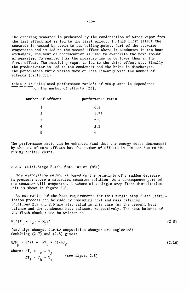
The entering seawater is preheated by the condensation of water vapor from the last effect and is led to the first effect. In this first effect the seawater is heated by steam to its boiling,point. Part of the seawater evaporates and is led to the second effect where it condenses in the heat exchanger. The heat of condensation is used to evaparate the next amount of seawater. To realise this the pressure has to be lower than in the first effect. The resulting vapor is led to the third effect etc. Finally the productwater is led to the condenser and the brine is discharged. The performance ratio varies more or less linearly with the number of effects (table 2.1)

table 2.1: Calculated performance ratio's of MED-plants in dependenee on the number of effects [23].

number of effects performance ratio

1 0.9

2 l. 75

3 2.5

4 3.2

5 4

The performance ratio can be enhanced (and thus the energy casts decreased) by the use of more effects but the number of effects is limited due to the rising capita! casts.

2.2.3 Multi-Stage Flash-Distillation (MSF)

This evaporation methad is based on the principle of a sudden decrease in pressure above a saturated seawater sol~tion. As a consequence part of the seawater will evaporate. A scheme of a single step flash distillation unit is shown in figure 2.8.

An estimation of the heat requirements for this single step flash distil­lation process can be made by employing heat and mass balances. Equations 2.5 and 2.6 are also valid in this case for the overall heat balance and the condenser heat balance, respectively. The heat balance of the flash chamber can be written as:

Mfc(Th - Tv) = MPL*

(enthalpy changes due,to composition changes are neglected) Combining (2.7) and (2.8) gives:

Q/M = L*(l + (~T + 6)/~Tî) p t

where: ~Tt = Tc

~Tf = Th (see figure 2. 8)

(2. 9)

(2 ,10)

-14-

FLASH CHAMBER

M s

:lrEMPERATURE

LOCATION

fig. 2.8: Schematic view of a single step flash-distillation mcthod,

Mf amount of feedwater [kg]

Mb amount of brine [kg]

M amount of produced freshwater [kg] p

M amount of cooling water [kg] c M amount of steam [kg]

s T ~emperature of the surroundings [K]

0

T g

T s

T V

temperature

temperature

temperature

of the

of the

in the

preheated feedwater

steam [K]

flash eh amber [K]

and the outgoing coóling water [K]

T c

temperature of the produced freshwater leaving the condenser fK]

Th temperature of the feedwater leaving the heater

o boiling point elevation [K]

-15-

The performance ratio can be written as:

L* T L* /q

0 = öTt+ê) T L*(l + 0

öTf

With: L* = 2442 kJ/kg T 0

L* = 2257 kJ/kg

öTt = 5 K

ê = 0.62 K

öTf = 50 K

the performance ratio is equal to 0.97. Again the performance ratio will have a value of the order of one. The most important reasons are: 1) the irreversible processes which result in entropy production 2) the heat which remains unused in the outgoing streams, The efficiency of this process can also be enhanced tremendously if more steps are used:multi-stage flash-distillation. The general scheme of this method is shown in figure 2.9.

The seawater, already preheated before entering the steamheater is heated to its maximum temperature. Then, the seawater is led to the first stage in which the pressure is lower than the vapor pressure of the seawater. As a result vapor is released from the seawater·and ledtoto a heat exchanger. in which it condenses. The heat of condensation is used for the preheating of the incoming seawater. The flow of seawater is led to the second stage which is at pressure which is lower than the saturation pressure of the seawater and vapor is relea~ed again etc.

Compared to the multiple effect distillation the amount of vapor produced in each step is much smaller. Therefore a multi~stage flash plant usually consists of more steps than a multiple-effect plant. Furthermore, the brine is often circulated, i.e. mixed with the incoming seawater, to achieve a large amount of productwater per amount of feedwater. But, what appears to be of more importance, this reduces the heat requirement. Due to this the performance ratio of multi-stage flash plants can reach values up to 12 and even more. This is done at .the expense of rising capita! costs but the rise in capita! costs with increasing number of steps is less than in the case of multiple effect plants because of the possibility for integrated constructions of multi-stage flash plants.

(2.11)

2

STEAM

3

STEAM 3

f!EATER

-16-

4'

5 6 1-r---r------_-_-----l- 6- - ~- - -

FIRST STAGE

SECOND STAGE

7

7

1 SEAWATER

8' FRESHWATER

BRINE

6

- ~ - - --- - -- FRESH-

FIN AL STAGE

9 WATER

SEA­WATER

fig. 2.9: General scheme and temperature diagram of a multi-stage flash­distillation plant. The numbers in the scheme and the temperature diagram correspond. Valves and pumps to maintain the required pressure and to remove non-condensing gases are omitted.

-17-

2.2.4 Vapor Campression (VC)

Vapor compression is an evaporation methad which uses mechanica! energy for the separation process. A schematic view is given in figure 2.10.

EVAPORATION­CONDENSATION CHAMBER

w

HEAT EXCHANGER BRINE

SEAWATER To

FRESHWATER T '----1-------11~ p

fig. 2.10: Scheme of a vapor compression evaporation method.

The entering seawater is preheated by the outgoing streams of brine and productwater. It is led to an evaporation-condensation chamber in which part of the seawater evaporates. The heat of evaporation is supplied by condensing watervapor which has been extracted from seawater and subsequently has undergone a compression. The process needs a starting heater but can operate without an auxiliary heat supply afterwards. The vapor-compression process can be illustrated by a temperature-entropy diagram of pure water (figure 2 .11).

The amount of mechanica! energy required for the process can be calcu­lated assuming the compression to be adiabatic. The required amount of work for the compression of watervapor from p to p is equal to:

v e

(J/mole]

where V denotes the rnalar volume. m

For an adiabatic compression one can derive the following relationship between the pressure and volume (ideal gas):

where k is the quotient of the constant pressure heat capacity and the constant volume heat capacity.

(2.12)

(2.13)

-18-

TEMPERATURE liquid vapor

liquid +

va por

ENTROPY

--fig. 2.11: Temperature-entropy diagram of pure water descrihing the w vapor-compression process.

Using (2.13) for the integration of (2.12) leads to an expression for the compression work per mole:

If pe-pv~ 1 (sma11 pressure change) then pv

( I ) Ck-1)/k Pe Pv

Substituting this in (2.14) gives:

w"' = pe-pv

RT _ __:.. V p·

V

0 If we substitute for pe the vapor pressure above pure water pw ,

and for p the vapor pressure above.the solution p both at the same V W

temperature we get:

(2 .14)

W ~ RT (p0 /p - 1) (2.15) V W W

0 Raoult's law states that p =x p (appendix B:(B.7)) where x is the water w w w w mole fraction. Then equation (2.15) can be written as:

-19-

1 1 xs \q = RTv(x- 1) = RTv(l-x - 1) = RTvl-x "' RTxs

w s s

where x is the salt mole fraction. s

The last term in (2.16) is equivalent with (2.3) which is the expression for the minimum amount of work required for the separation. The actual energy consumption is higher because: 1) The increase in pressure (and consequently the·· temperature difference)

has to be larger in order to achieve a reasonable level of heat exchange in the evaporation-condensation chamber.

2) The compressor efficiency is not taken into account. 3) Heat and friction losses are neglected.

2.3 Freezing methods

In a seawater salution which is cooled to its freezing point ice-crystals consisting of pure water will develop. These ice-crystals can be separated mechanically from the mixture of brine and ice. If the ice is then melted freshwater becomes available. Most of the freezing methods use mechanica! energy. They make use of a refrigerant to reach the desirabie low tempera­ture. In case of direct heat exchange between the refrigerant and the sea~ water the freezing method is called a direct freezing method. Instead, if the heat is exchanged via an interface, the freezing method is called indirect. Three methods (2 direct, 1 indirect) will be discussed in this section.

_First, a direct freezing method using water itself as a. refrigerant is d1scussed. A schematic diagram of this process which is often referred to as the vacuum-freeze vapor compression process or the "Zarchin process" is shown in figure 2.12.

COMPRESSED VAPOR

COMPRESSOR

Ir V ACUUM

I ~ "' PREEZING SEPARATION

eH AllEER UNIT EL TER

I I

ICE + BRINE -FRES:!WATER

FRESHW ATER

BR INE 1 - 1--HEAT EXCHANGER ... FRES:fWATER

I

SEAWATER

(2.16)

fig. 2.12: Schematic view of the vacuum-freeze vapor compression process [14]

-20-

Caoled seawater is led to a. freezing chamber which is kept at a tempera­ture near the freezing point (or rather the triple point) and a pressure which is lower than the saturation pressure of the incoming seawater. Part of the seawater evaporates and extracts the heat of evaporation from the seawater in which consequently ice-crystals will develop. The water vapor is compressed by which it rises in temperature and then led to the melter in which it serves to melt the ice. The slurry of ice and brine leaving the freezing chamber is led to the separation unit which separates the entering stream into two streams of brine and ice. The brine is discharged via a heat exchanger which cools the incoming seawater. The ice is transported to a melter in which it is melted by the heat of condensation of the water vapor. The resulting freshwater is led to the heat exchanger to cool the incoming seawater, but part of is led to the separation unit to wash the ice-crystals.

Another direct freezing method, called the secondary refrigerant process, uses a refrigerant (iso-butane) which is inmiscible with seawater. This process is illustrated by figure 2.13.

I SOBUTANE V APOR COMPRESSOR COOLER

~

LIQUID ISOBUTANE MELTING FREEZING ISOBUTANE SEPARATOR WATER CHAMBER +

ISOBUTANE UNIT

FRESHWATER -

ICE

SEPARATION ICE + BRINE UNIT

~ ~ SEAWAT ER

I :tWATER FRES: .. '--

COOLED -SEAWATER HEAT EXCHANGER

BRINE I

fig. 2.13: Schematic view of the secondary refrigerant process [14].

Caoled seawater is led to the freezing chamber in which it is mixed with liquid iso-butane. The refrigerant iso-butane evaporates, thereby extracting its heat of evaporation from the seawater in which consequently ice-crystals will develop. The iso-butane is compressed, as a result rises in temperature and is led to the melting unit. T\e slurry of brine and ice which leaves the freezing chamber is led to the separation unit. The resulting ice is transported to the meiter in which it is mixed with the iso- butane and melts. This mixture is led to the iso-butane separator which separates the freshwater from the iso-butane. Again, part of the freshwater produced is used to wash the ice-crystals in the separation unit. The rest of the freshwater and the brine leaving the separation unit is led to the heat exchanger in order to cool the incoming seawatèr.

-21-

The last freezing method to be discussed is the indirect freezing method. It is illustrated by figure 2.14.

j ~COMPRESSOR I ~ COOLER I

I . . .. J I

LIQUID REFRIGER~IT

I ICE L ___

'----FREEZING t.:ELTING CHAMBER UNIT

FRESHWATER ,.

I .

FRESHWATER

' SEPARATION UNIT

ICE + BRINE

SEAWATER

L -I -.. FRESHWATER HEAT EXCHANGER ..

BRU:E I BRINE

fig. 2.14: Schematic view of the indirect freezing method [14].

The processes of freezing, separation and melting are analogous to the aforementioned direct freezing methods. The main difference is the use of a closed freezing system, its refrigerant having no direct contact with the seawater. Having discussed the direct freezing method figure 2.14 speaks for itself.

The use of low temporature separat~on processes has several advantages over the high temperature processes (distillation): 1) Lower rate of heat exchange per unit of product because the heat of

fusion is approximately one-seventh of the heat of evaporation. 2) Less sealing problems (sealing is the precipitation of certain

constituents of seawater for instanee on heat exchangers~ 3) Less corrosion problems. 4) Use of less expensive materials. But, employing freezing methods for desalination of seawater also has some disadvantages: 1) Several processes, for instanee the vacuum-freezing vapor compression

process, have to be operated at extremely low pressures. 2) An external refrigeration system is usually necessary to cancel the

heat leakage into the plant. 3) Productwater is lost due to the washing of the ice-crystals in the

separation unit.

Furthermore, for the sake of completeness the hydrate processes are mentioned here as processes similar to the freezing processes. Hydrates are clusters of watermolecules arourid a water attracting molecule or ion.

-22-

The use of hydrates may allow the formation of ice-crystals at tempera­tures higher than the freezing point. The lay-out of a hydrate process is more or less the same as a freezing process. But as a matter of fact the hydrate processes do not p1ay an important ro1e in seawater desalination.

2.4 Membrane methods

2.4.1 E1ectro-dia1ysis (ED)

The first of the separation.methods to be discussed which use semi­permeab1e membranes is e1ectro-dia1ysis. This process which requires an electrical energy input is i11ustrated by figure 2.15.

BRINE PRODUCTWATER BRINE

.J (+) 1 CBED$$$ "6l ft' eeaaa

~

$Ci~SEB e;r $ a eeeea ELECTRIC J

e , (i e E8 E9 a ED e e e

J

' ' CURRENT 5 'i • eEBeee 9 a a ..._.

"' ~ .. I

e • $G~6$ e e Jl ."

I

ELECTRODE MEMBRfu~E MEMBRANE

SEAWATER SEAWATER SEAWATER

fig. 2.15: Principle of the e1ectro-dia1ysis process. (+) membrane which is permeab1e to positive ions only. (-) : membrane which is permeab1e to negative ions only.

E9

-23-

An electradialysis unit consists of a number of compartments which are separated by alternating kinds of special membranes which are separated by alternating kinds of special membranes which are permeable to positive ions (+) or negative ions (-) respectively. (this is called a stack; see figure 2.16). If an electric field is applied transverse to the membranes the ions will start to migrate as shown in figure 2.15. Positive ions will migrate through the membranes which are permeable to positive ions, negative ions will migrate through the membranes which are permeable to negative ions. After the ions have passed the first membrane it is un­likely they will migrate through the second one because that one is only permeable to ions of the opposite charge. The result is the separation of an incoming stream of seawater into a concentrated one (brine) and a diluted one (freshwater) (see figure 2.16)

CONCENTRATED CONCENTRATED

t

t

. .

·. I • • • : ••• t • • . . . ... . .

!• •• '

t

t

•'• :.-,· '• . , . . . -: . . . . . . . ,. '·. ...... , .

t

SEAWATER

t t

fig. 2.16: Schematic representation of the separation process in an electrodialysis-stack.

r

The mechanism which determines the permeability of the membranes to either positive or negative ions is based on ion-exchange. It appears that for instanee the positive ions can move more or less freely inside the membranes which are permeable t'o positive ions. The negati ve ions on the other hand are more less fixed inside the membrane.

If a seawater salution is brought in electrical contact with pure water a voltage difference will establish itself between the liquids. This voltage is related to the minimum amount of energy required for the separation of seawater into brine and freshwater and it opposes the process of electrodialysis. The voltage neéded to operate an electrodialysis-stack effectively must have a value which is higher than this offset-voltage. In practice the voltage will be higher because of: 1) the economical necessity of a reasonable level of the productwaterflow. 2) the dissipation losses due to the resistance of the salution and the

membranes.

-24-

3) polarisation. At the wembrane surfaces the concentration of ions will differ from the bulk concentrations. A simplified diagram of the concen­tration profile is shown in figure. 2.17.

CONCENTRA TI ON

/~1 /coNCENTRATED. \

I

~ (-)

+ ELECTRIC FIELD

fig. 2.17: Simplified diagram of the concentration profile near the membranes [23].

The existence of a concentration gradient over the membranes gives rise to an increase in resistance of the electrodialysis-unit. This can be understood by realizing that diffusion processes which result from the concentration gradient oppose the direction of flow of the ions caused by the electrical field. Furthermore the increased concen­tration near the membrane surface may lead to precipitation of certain seawater constituents on the membrane.

2.4.2 Reverse Osmosis (RO)

The second membrane method for seawater desalination to be discussed will be reverse osmosis or hyperfiltration as it is often called. The phenomenom of natura! osmosis, which plays an important role in the selective transport of materials in the world of nature is illustrated by figure 2.18a. If a salution consisting of a solvent and one or more solutes is separated from the pure solvent by a semi-permeable (which is permeable to the solvent only), the solvent will start to migrate to the salution as a:result of the concentratien difference (or rather difference in the chemica! potential). This flow of solvent will decrease if an external pressure is applied to the solution. The pressure at which no net flow of solvent occurs is called the osmotic pressure ~ (equal chemical potential on either side of the membrane)(figure 2.18b). If the pressure is increased above the osmotic pressure the flow direction of the solvent will reverse and solvent will flow from the salution to the pure solvent (figure 2.18c).

.... ·' ·: :· . • • I • ... . . . . . . .. . · .. ·.·· ... . . . .. . . . ... ,..._..,.._. ~/'·i.:.· 'i :~ .. .,;·.·=·~~:r--

" MEMBRANE

a:natural osmosis (net flow)

-25-

1t

MEMBRANE

b:thermodynamic equilibrium

(no net flow)

fig. 2.18: Osmotic principles.

P~n)

lVIEMBRANE

c:reverse osmosis (net flow)

An expression for the osmotic pressure for ideal mixtures of two componentsis derived in appendix B (Van 't Hoff's law:(B.l4))

RT lT=--x V s mw

where: R = universa! gas constant [J/(mole K~ T = temperature [K] x = -sal t mole fraction

s 3 V = molar volume of water [m /mole] mw

Thus the work required for the transport of one mole of water across a pressure difference 1T is equal to:

RTx [J/mole] s

This is equal to the absolute minimum amount of energy required for the separation as given in (2.3).

Reverse osmosis will be discussed more extensively in chapter 3.

2.5 Comparison of desalination methods

In this section the desalination methods presented in the previous sections will be compared one with another. The following factors will be included in the comparison: 1) Energy consumption per amount of freshwater produced 2) Investment costs per installed daily capacity 3) complexity, start-up, operation and maintenance of the plant 4) pretreatment 5) productwater quality

(2 .17)

-26-

1) Energy consumption

In table 2.2 the 3pproximate energy cons~mptions per amount of produced freshwater [kWh/m ] are presented for several desalination methods. Also the m1n1mum amount of energy required for the separation of seawater and the ~eat of evaporation and fusion are given.

table 2.2: Energy consumption of several seawater desalination methods [27],[28]. -Right numbers refer to proven energy consumptions in existing plants; -Left numbers refer to processes which are commercially available but yet nat proven in the field.

-SP:single purpose i.e. water production only. -DP:dual purpose i.e. electricity production, low pressure steam is used for waterproduction.

-f:based on fossil fuels -e:electrical or mechanica! energy

Multi-stage flash

Multiple effect

Vapor compression

Reverseosmos is

Electra-dialysis

Freezing

Abs. min. am. of en.

min. am. of en, (0.5 conv.)

heat of evaporation

heat of fusion

66(f)/98(f) 2

73(f)/12l(f)3

12(e)/16(e)

8(e)/12(e)

30(e)/ -

16(e) 4

0.71

0.99

630

93

33(f)/4l(f) 2

3l(f)/47(f) 3

Notes: 1: These energy consumptions are based on the fact that in the SP-process the necessary steam wil! be high pressure steam whilst low pressure steam is used for the OP-process. It is assumed that the amount of fossál fuel needed for the production of low pressure steam is 0.35 of the amount of fossil fuel needed for the production of high pressure steam. The amounts of energy given in the table also include pumping work (electricity which is generated with a conversion efficiency of 0.34 with respect to fossil fuel).

2: low numbers refer to acprocess of performance ratio equal to 14; high numbers refer to a process of performance ratio equal to 8.

3: low numbers refer to a process with 7 effects; high numbers refer to a process with 12 effects.

4: pilot plant.

It is expected that the freezing methods wil! reach an energy consumption

of about 13 kM1/m3. But at present this methad is not widely used as a result of their high investments [14]. Compared to reverse osmosis and vapor compression electra-dialysis is a high energy consuming process (it appears that the energy consumption is approximately proportional tothesalt concentration). Furthermore,

-27-

the technique has yet not been proven to be economically feasible for seawater desalination. For desalination of brackish water, though, electra-dialysis appears to be competitive with reverse osmosis [29,30,31]. Finally it is worthy to mention the following: The distillation methods operate via an exchange of heat equal to that of evaporation whereas the freezing methods operate via an exchange of heat equal to that of fusion, Assuming the same loss-fraction the losses are in terms of energy units much larger in the case of distillation. Heat losses play no role in processes which operate at ambient temperature (reverse osmosis~

2) Investment casts

The dependenee of the (1979) investment costs per daily capacity on the plant capacity is shown in figure 2.19 (32] for several widely used seawater desalination technologies.

INVESTMENT COSTS [$/(m3/day)] ~

1500

1000

500

\ ~ '~ t1S

" ~ L

"' I ......

~ 1-o.

~ - ...........

Rb Mi .......... ........

r-...

Q5 1 2 5 10~ 50100200 PLANT CAPACITY [lOOQ:,m3 /day]

1979

prices

fig. 2.19: Dependenee of the investment casts per daily capacity on plant capacity for reverse osmosis and distillation methods. (MSF=multi-stage flash; ME=multiple effect; RO=reverse osmosis)

Vapor compression investment casts are approximately the same as the reverse osmosis investment casts [29,33]. Note-worthy is the fact that the "economies of scale" apply less to reverse osmosis than to multiple effect and multi-stage flash-distil­lation, The modular build-up of a reverse osmosis plant may be credited for this. Compared with reverse osmosis multiple effect and multi-stage flash distillation investment casts are higher in the low capaci ty range but lower in the high capacity range,

3) Complexity, start-up, operation and maintenance

Finnegan and Wagner have compared several desalination methods (reverse osmosis and distillation methods) [34]. They analysed the start-up sequence and oparation of several kinds of plants (of a certain average capacity which they do not mention explicitly) and concluded that reverse osmosis was the easiest to start-up and opera te. One of the most interest ing.,. features is the fast start-up time of 1/2-1 hour for a reverse osmosis plant. This compared to 2-4 hours for distillation plants, Furthermore an analysis was made of the complexity of desalination plants based on the comparison of the numbers of controls, alarms, chemica! systems,

-28-

other systems and pumps. It favored reverse osmosis as the easiest. Vapor compression was the most complex desalination method according to them. As far as maintenance was concerned they ranked multi-stage flash on the first place (i.e. least maintenance), foliowed by reverse osmosis, multiple­effect and vapor·compression but admitted they had not much experience with reverse osmosis maintenance .. The results of Finnegan and Wagner concerning the reliability and simplicity of reverse osmosis plants are supported by Bushnak et. al. [35]. The latter mention another interesting feature of reverse osmosis plants viz. the relatively easy possibility of capacity expansion

4) Pretreatment

Pretreatment of the entering seawater is essential in every desalination plant to maintain a certain desirabie waterproduction rate and ·to ensure a durable operation of the plant. The main objective of pretreatment is to prevent sealing i.e. the precipitation ;of certain seawater constituents. The salts which are most liable to precipitation are Caso

4 (especially at

high temperatures), MgO and Caco3

[23]. Sealing causes a decrease in

heat transfer in the heat exchangers of a distillation plant and membrane fouling in reverse osmosis plants. Several methods have been developed to prevent unwanted precipitation: l) An appropriate design of the desalination plant so as to avoid conditions

at which precipation can occur. 2) Removal of possible precipitators before the separation process. 3) Addition of chemieals to prevent or to retard precipitation or to

cont:o~ th~ precipitation e.g. acid addition will avoid MgO ana Caco3 prec1p1tat1on.

4) Controlled precipitation in certain regions. In case of reverse osmosis plants special care has to be taken with respect to fouling of the membranes. Finally, every desalination plant· possesses one or more filtrations to remove suspended particles.

5) Productwater quality

The distillation methods deliver freshwater with a salt content below 50 ppm whereas by single step reverse osmosis the productwater salt concentration is only a few hundreds of ppm's.

2.6 Selection of a desalination method

In this section a desalination method which is suited for the application of windpower is chosen. It is stipulated that the desalination method has to be a proven desalination technique in the field. Thus, electro-dialysis and the freezing methods arenottaken into consideration.This leaves reverse osmosis and the distillation techniques. Furthermore, starting from proven desalination techniques restricts the research to the matching problem of the desalination plant and the windturbine only.

One of the most characteristic properties of a windturbine is its power variation (long term and short term) due to the windspeed variations. It is assumed that no long term storage (days) is used to cover the periods of insufficient windpower. But, short term (minutes-hours) in the available windpower may be covered for by a battery unit.

-29-

Unfortunately, extensive information about the unsteady operation of desalination plants is lacking. Only two· references have been found [36,37] which deal with this problem to some extent. In these papers results are given of the unsteady operation of a brackish water reverse osmosis plant. The experiments were done by applying. a sinusoidal variation in the feecl­water supply at constant pressure to the reverse osmosis unit. According to the experimenters this .did not cause any extra difficulties compared to the steady operation. But, it should be mentioned here that the variations in the feedwater supply (and thus in the power supply) were fairly small: + 30%.

Despite the incomplete knowledge on the unsteady behavior of desalination plants it is possible to choose a desalination technique based on the in­formation presented in the former section. Multi-stage flash and multiple­effect plants are excluded because of their high energy consumption (appr. a factor 8-10 higher than reverse osmosis; taking into account the energy-efficiency of the electricity generation the difference remains substantial(appr. a factor 3). In fact it is generally believed that multi­stage flash and multiple-effect plants can only be competitive when combined with electricity production (dual purpose) [30]. The choice between vapor compression and reverse osmosis can be made on the basis of the operational ease of reverse osmosis plants (less complex, less maintenance, fast start-up, easy operation) in favor of reverse osmosis. Furthermore,the expected future developments seem very favorable for reverse osmosis because of the rapid development of the membrane technology and the development of techniques to reeover energy from the high-pressure brine which leaves a reverse osmosis plant. Reverse osmosis will be discussed more extensively in the following chapter.

Note:This chapter was mainly basedon [14,23,15,38,39].

-30-

3. ASPECTS OF REVERSE OSMOSIS*

3.1 Historica! background

In 1748 abbé Nollet first discovered the phenomena of natura! osmosis and selective transport properties of membranes when experimenting with animal bladders. Approximately two centuries later it was Reid (University of Florida, USA) who suggested the use of semi-permeable membranes for the desalination of salty solutions. During the 1950's the attention of the researchers was focused on the development of adequate membranes. Their research task was to develop membranes.which would be highly permeable to water and highly impermeable to the solutes. Furthermore these membranes had to be very thin to assure a reasanabie flow of productwater while meeting the demands of mechanica! strength and they had to be chemically inert to the salty solutions and finally the membrane area to volume ratio had to be as high as possible [40]. In 1960 Loeb and Sourirajan introduced the asymmetrie cellulose-acetate membranes which proved to be of practical use for desalination processes (figure 3.1)

0.2 microns

carrier material

fig. 3.1: Asymmetrie cellulose acetate membrane [41].

It lasteduntil 1967, however, befare the first commercial (brackish water) desalination plant was installed. The development of membrane technology in the past 20 years is illustrated in figure 3.2 showing the development of the water permeability of seawater membranes (the permeability is defined as the waterflux per unit of membrane area per unit of effective pressure difference across the_mêmbranes [m 3 /m~day.MPa]) This rapid development of membrane technology is also reflected in figure 3.3 which shows the yearly installed brackish water desalination capacity in the world. In the Netherlands reverse osmosis plays an important role in the pre­paration o! irrigation water for greenhouses from salty surface waters. The first commercial seawater desalination plant was installed in 1975 in South Caicos (British West-!ndies) to cover the water supply of a hotel. In 1980 the reverse osmosis seawater desalination capacity was estimated to be 40000 m3/day which is very small compared to the brackish water capacity but it is generally believed that it will increase very

* Reverse osmosis is aften referred to as hyperfiltration to stress the link between (or rather extension of) other filtration processes like micro- and hyperfiltration. Because of the differences in separation ; mechanisms between reverse osmosis and filtration and because of the thermadynamie properties involved the idea of reverse osmosis will be used in this report.

permeability

xlO (m3/m2d.MPaJ

3.0

2.5

2.0

1.5

1.0

0.5

•• •

• • •• ••

••

-31-

•• •

•

o~~------~--------~-'60 '70 '80

year-..+

fig. 3.2: Development of seawater membrane performance [41].

capacity mtday(x10 3

)

500

'70

years

fig. 3.3: Yearly installed brackish water RO-plant capacity [43].

rapidly in the future [42]. At the end of 1983 it was estimated to amount to 110000 m3/day. The commercial breakthrough of reverse osmosis being apparent, the research efforts to improve the selective transport properties of the membranes is carried on.

-32-

3.2 Mechanisms of membrane separation processes

It is not the objective of this section to give an extensive account of all processes which are taking place near and in the membrane but merely to illustrate these processes. For a review of the RO transport models, which is beyond the scope of this study, the interested reader is referred to (44]. The selective permeability of a membrane to solutes lsalts) and solvent (water) is determined by two properties viz. the solubility of salts and water into the membrane and the diffusivity of salts and water inside the membrane. The two most used membrane materials for desalination purposes are cellulose acetate and aromatic poly-amide. The solubility of salts into cellulose acetate membranes is much smaller than in aromatic poly-amide membranes but on the other hand the diffusi­vity is of salts is much higher in the case of cellulose acetate membranes. As a result the salt permeability of both membranes is approximately the same (44]. Furthermore a third property has tobetaken into consideration i.e. the fact that the membranes are "lea.ky". As a consequence, the convective transport of salts may play an important role also. In figure 3.4 a general picture is shown of the transport through an asymmetrie membrane.

I• ltl111brane

f c,

Dt1111 Skl1 La.rer t

Porous Support High Pressure Loyer c~. Side

c,

fig. 3.4: Schematic representation of the saltconcentration-profile in and near an asymmetrie membrane (44]. C~b : salt concentration in the bulk of the solution

C' .sw : salt concentration on the outside of the membrane surface (feedwater­

(C' ) :salt concentration sw m (feedwaterside)

on the inside of the membrane surface

(C" ) :salt concentration on the inside of the membrane surface sw m

side)

(productwater­side)

-33-

In figure 3.4 5 regions which are of interest to the separation process are depicted:

a: Bulk region This region represents the seawater in the main stream with an uniform salt concentration C~b'

b: Boundary layer Due to the solvent (water) extraction the concentration of salts will increase near the membrane surface (concentration polarisation). This effect will be discussed in the next section.

c: Surface region (transition between fluid and membrane) This region is identified by two processes: 1) diffusion of solutes along the surface due to membrane imperfections 2) adsorption of solutes into the membrane The differences in solubility and diffusivity of solvents and solutes in the membranes cause a sharp decrease in salt concentration.

d: Skin layer This dense region is characteristic for asymmetrie membranes. lts existence causes the salt rejection.

e: Porous support region This region serves as the support of the skin layer. As it has no salt rejecting properties the concentration profile remains flat in this region.

Several descriptions of the salt rejection mechanism exist, for instanee the ordinary sieve mechanism which is based on the difference of molecular size between solvent and solutes. This mechanism is ignored in reverse osmosis because solutes and solvent molecules or ions are of approximately the same si ze. (14] . Furhermore a model which assumes the existence of a layer of water on the membrane surface has been developed (wetted surface mechanism). The selective properties arise from the fact that water molecules will be absorbed easily by this layer but solutes have to overcome the strong hydragen honds in the layer. A third mechanism to describe the salt rejection is the preferential sorption capillary flow mechanism. There exists a.link with the phenomenom of surface tension:The interface between a salution and free air exhibits a lower concentration of solutes than the bulk of the solution. In an ana­logous way this is also expected to take place at a membrane-solution interface (figure 3.5a)

l'kl~~UJ(l.

I Hz{J .... Cl. Hl(l -.•cl· HzO

• 1o .":"'c1· .. •J~. ~·c·~ .. •?o

a b fig. 3.5: Schematic representation of the preferential sorption-capillary

flow mechanism [45].

-34-

The interface consists of a layer of water molecules. The membrane is assumed to possess micro-pores. The transport of solvent takes place under pressure via capillary processes through the pores which have to be of a certain critica! size to optimize waterflux and salt rejection (figure 3,5b) Finally a fourth mechanism should be mentioned namely the solution­diffusion mechanism. This model assumes the membrane to be non-porous. As a consequence the transport of solutes and solvent,is purely basedon solubility and diffusivity of solutes and solvent in the membranes. This model has been modified by assuming pores do exist on the membrane surface (solution-diffusion-imperfection models or other models like friction models, combined flow-diffusion models). This modification was necessary since besides the mechanisms of solubility and diffusivity, the conveetien mechanism also plays an important role. Especially the transport of solutes appears to be dependent r · on the convection.

In the next sectien a simple linear model of the membrane separation process is presented. This model appears to describe the separation process surprisi~gly well.

3.3 Simplified description of the RO-plant performance [46,47]

The driving force for the separation process is the difference in chemica! potentials of solvent (water) and solutes (salts) between the solutions on either side of the membrane. This difference arises from the difference in pressure and concentration.

The separation process is depicted schematically in figure 3.6.

fig. 3.6: Scheme representing the essentials of an RO-plant.

An entering feed flow Ff (seawater) with salt concentration Cf is separated

into two flows: one concentrated Fb·(brine) with concentration Cb and

the other diluted F (productwater) .with concentratien C • p p

-35-

The separation process can be described by a simple linear model in which the flow of water through the membrane F is approximated by the

w following equation:

F = a(~p - ~n)A w m 3 [m /s] or [1/s]

where: a = membrane constant (which is a weak function of the pressure) ~p = hydraulic pressure difference between the feedwater and the

productwater, which is equal to pf-pp (pf and pp are the

pressures of feedwater and productwater respectively,relative to ambient pressure)

~n = osmotic pressure difference across the membrane A = membrane area m

~p - ~n represents the effective pressure drop across the membrane.

The flow of salts across the membrane F can be approximated by: s

F = b~CA [mg/s] s m

where: b = membrane constant(which is a weak function of pressure and feedwater concentration)

~C = salt concentration difference across the membrane A = membrane area m

It is customary to express the ability of the membranes to reject salts by the salt rejection r:

r = (C - C )/C f p f

where

water Using

Cf and CP are the salt concentrations of the feedwater and product­

respectively [mg/1 ]. the relationship C =F /F and equations 3.1 and 3.3 we can write:

p s w

r = a(~p - ~n) a(L'!p - L'!n) + b

The salt rejection is both depend~nt on osmotic pressure and operating pressure. The osmotic pressure increases along the membrane surface because of the continuous water extraction. The concentration on the feedwaterside in the membrane varies from the feedwater concentration Cf to the brine concentration eb. Assuming the

salt rejection to be constant the concentration of the water produced wil! vary from (1-r)Cf to (1-r)Cb (using equation 3.3). The water

produced is pooled to give a single flow with an average concentration equal to C . Because the salt rejection is assumed to be constant:

p

CP = (1 -r)Cf

where:Cf = the average concentration on the feedwaterside.

It is possible to derive an expression for CP in dependenee of Cf under

the assumption of constant salt rejection.

(3.1)

(3. 2)

(3. 3)

(3.4)

(3.5)

-36-

From the conservation of salts:

the definition of the conversion Y:

Y = Fp/Ff

and the conservation of water:

F f = Fb + F p (assuming the flows to have equal density) one can write for the salt concentration in the outgoing brine:

C - YC c = f p b 1 - y

During the separation process the fraction of extracted water will increase from 0 to Y. We will define the local conversion y as the paoled amount of productwater at a certain location in the membrane module divided by the original amount of feedwater Ff i.e. O~~Y.

The salt concentratien on the feedwaterside at this location is called CfCy). The salt concentration of the paoled producth•ater is called CJ,CY)

at this point. In figure 3.7 the concentratien profile on the feedwater­side is depicted as a function of the local conversion y. The fat line is a schematic representation of the membrane.

FEEDWATER 1 PRESSURIZED FEED CONCENTRAT ION I (C I) I I

f I (' I I f _____. • Cb.'Fb

Cf,~ al I I

----t I

I I

I I MEMBRANE I

I

• CP, Fp : c' I I p 14 _, I I

0 y y LOCAL CONVERSION (y) •

fig. 3.7: Concentratien profile on the feedwaterside as a function of the local conversion.

Analogous to equation 3.9 we can write for the salt concentratien on the feedwaterside (constant salt rejection):

C{(Y) = Cf - yCP(y) 1 - y

(This can be understood as a membrane module operating at conversion y)

The salt concentratien of the locally produced water at a point where the local conversion equals y can be expressed as:

(3. 6)

(3.7)

(3.8)

(3. 9)

(3.10)

-37-

(1 - r)C:f (analogous to 3.5)

The concentration of the pooled productwater is the average of every membrane portion up to the point where the local-conversion equals y. This can be written as:

C'(y) = ~ JY(l-r)C'(y'ldy' p y 0 f / (3 .11)

Substitution of (3.11) in (3.10) gives the salt concentration onthefeedwater side at the point where the local conversion equals y:

JY(l-r)C' (y')dy'} 0 f

(3.12)

or

Differentiation with respect to y gives the following differential equation:

dC:f r dy = 1-y

Integration between the boundaries o and Y, Cf and Cb gives:

-r Cb = Cf(l-Y)

Substituting this result in equation 3.9 and solving gives an expression for C :

p l - (1-Y)l-r

CP = Cf y

This result is plotted in figure 3,8 as a'function of y for several values of r which are valid for the high rejecting seawater membranes. The salt rejection of these membranes must exceed 0.985 to meet the WHO-limit of 500 ppm for the productwater, if the feedwater is average seawater (34500 ppm). From figure 3.8 one can learn that increasing the conversion leads to

(3 .13)

(3.14)

(3.15)

an increasing salt concentration in the productwater (constant salt rejection) The energy consumption per amount of product water is equal to:

Plf pf -F- = y

p (usually expressed in kWh/m3)

where: pf = difference between feedwaterpressure and ambient pressure

Ff = feedwater flow

F = productwater flow p

Y = conversion

Thus, increasing.·y leads to an enhanced energy-efficiency of the seawater separation at the same operating pressure.

According to (3.1) an increase in pressure gives rise to an enhancement in the amount of productwater. However, there exists an upper limit to the pressure caused by the danger of mechanica! deterioration of the membranes. Lowering the pressure at constant feedwatér flow re sul ts in an increase in the productwater's salt concentration because unlike the salt flow through

(3.16)

-38-

0.04 cpjct r::0.985

0.03

r = 0.990 0.02

0.01 r .=0.995

0 CONVERSION

0 0,1 0,2 0,3 0,4 0,5 0,6 0,7 0,8 0,9

fig. 3.8: Salt concentration in the productwater as a function of the conversion for several salt rejections,

the membrane the water flow through the membrane declines. Thus also a lower limit is imposed on the operating pressure.

1,0

Typical values for the conversion Y, operating pressure pf, salt rejection r and the energy consumption per amount of productwater in case of seawater desalination are given in table 3.1.

table 3.l:Some typical values of RO-plant parameters.

Conversion Y

Operating pressure

Salt rejection

Energy consumption

0.25 - 0.30

50 - 70 bar

>0,985

8 kWh/m3

Änother troubling feature in membrane separation processes is concentration polarisation. This is the effect of increased concentration of salts (higher than the bulk) in the membrane surface as a result of their rejection. Concentration polarisation is undesirable for several reasons: 1) increase in osmotic pressure which results in a lower water flow through

the membranes, 2) higher salt flow through the membranes. 3) precipitation of certain seawater constituents on the membrane surface. Problems arising from concentration polarisation can be reduced by a proper pretreatment of the feedwater, enhancement of the veloeities along the membrane surface and lowering of the conversion.

The performance of two commercially available membranes wil! be discussed in section 3.5.

-39-

3.4 Reverse osmosis plant description

In figure 3.9 the general scheme of an'RO-plant is depicted. The incoming seawater is first pretreated to minimise/eliminate possible precipitation of seawater constituents and to control the chemica! and biologica! compo­sition of the feedwater in order to minimise membrane deterioration. After the pretreatment the seawater is fed to the membrane modules where it is separated into·brine and freshwater. Quite often the freshwater has to undergo a post-treatment (not indicated) to bring it up to the desirabie drinking water standards. By energy-recovery the reverse osmosis process can be made more energy-efficient: energy available in the pressurized brine is reeavered and can be either used for the pressurisation of the incoming seawater or for other purposes outside the plant,

FEED­WATER

PRETHEATMENT

HIGH-PRESSURE p~p

ENERGY RECOVERY

BRINE

fig. 3.9: Lay-out of areverse osmosis plant.

MEMBRANE MODULES

PRODUCTWATER

The components of a RO-plant will now be discussed starting with the main one, the membrane module.

Membranes

The materials commonly used in commercial asymmetrie membranes are polymers either cellulose-acetates or poly-amides, Besides the semi-permeability the membranes have to possess several other properties: 1) Resistance to compaction,

Compaction is the effect of compression of the membrane skin layer as a consequence of the continuous exposure to the high pressure, This effect which is larger for high pressures and high temperatures gives rise to a decline in the water flow through the membranes and an in­crease in salt rejection.

2) Resistance to fouling. 3) Resistance to bio-degradation.

e.g. Poly-amides are highly resistant to bio-degradation; cellulose­acetates somewhat less, so in this case chlorine is often added to the seawater as a pretreatment.

4) Resistance to chlorine and other chemicals. e.g. Poly-amides are affected by a high chlorine concentrations.

-40-

5) Stability in a wide range of the pH. 6) Stability in a wide temperature range.

In the past years several geometries have been developed for the membranes: 1) Plate and frame device

Membranes in flat sheets are laid on each side of a porous plate These plates are arranged in a stack inside a pressure vessel. The seawater is supplied under high pressure on the outer side of the porous plate: Water is pressed through the membranes to the porous plate where it can flow to a collecting point. The flow pattern is depicted in figure 3.10.

Membranes SaltWater

... ,·.·.: .. · .. · .· .. : ... ,.' -·.· :'·":. · ... · ...... ~ ... ~.: .. -... -

fig. 3.10: Flow pattern in a plate and frame module [48].

The concept has lost favor in recent years because of its low membrane area to volume ratio (compared withother devices). Therefore a large pressure vessel is necessary. Nevertheless, still some interest in the plate and frame device exists in the plate and frame device [49].

2) Tubular devices In this device the membrane is a coating on the inside of a porous tube. Seawater is supplied under pressure at the inside of the tube and consequently freshwater is produced on the outside, This principle is shown in figure 3.11.

Practical Unit

Pump

Fresh Water

fig. 3.11: Tubular reverse osmosis device [48]

•

Brine Concentrale

Out

-41-

The tubular devices have a low rnernbrane area to volurne ratio. On the other hand, rernoval of particles present in the feedwater is not necessary and cleaning of the membranes is fairly easy. But their high costs makes thern incornpetitive in seawater desalination cornpared to the following two devices. In case of wastewater conditioning the tubular devices rnay play an important role.

3) Spiral wound device This device is built up frorn two flat membranes laid tagether and glued on three sides to forrn an envelope. The open side of the envelope is fixed over a slit found alóng the length of a tube. Mernbrane with spaeer are wrapped around the tube to forrn an element. A module consists of a few of these elernents. The feed water flows frorn one side in an element along the rnernbrane parallel to the central tube and ernerges as brine on the other side. The productwater flows through the porous material between the membranes into the central tube [41]. Figure 3.12 gives an idea of the spiral wound device.

Product Water

brine

Product Water Flow (alter Passage

through Membrane)

Product Water Side Backing with Membranes

on Each Side

fig. 3.12: Spiral wound device [48].

Feedwaler Flow

Product Tube

End view

The rnernbrane area per volurne ratio is approxirnately 1000 rn2;rn3 which is ten tirnes higher than for a tubular device,

4) Hollow fibre device The membranes in this device consist of hollow fibres of a thickness ~f about 0.1 rnm. These fibres have a dense skin on aporous supporting layer (figure 3.13).

TI1e feedwater is supplied to the outer side of the hollow fibres and freshwater consequently perrneates to the inside of the hollow fibre. A perrneator which consists of about a rnillion hollow fibres is depicted in figure 3.14. The rnernbrane area per volurne ratio is about 10000 rn2;rn3 which is ten tirnes higher than a spiral wound device, But the flow per rnernbrane area is less. In seawater desalination the last two devices are favored despite the necessity of an extensive pretreatrnent.

-42-

t51J. OD

fig. 3.13: Dimensions of a hollow fibre (PERMASEP BlO permeator)

fig. 3,14: Hollow fibre permeator [50].

~~~~-EE~~~~E~-E~~E~

FEED DISTAIBUTOR TUBE

The pumps used in an RO-plant are either centrifugal or positive displacement pumps. For small plants positive displacement pumps are favored because of their high efficiency. On the other hand the advantage of centrifugal pumps is their low maintenance requirement. In figure 3.15 the approximate domains of operation are depicted.

1 ul. --

PRES- b 7 SURE 0

5

[oar] 4

L '

I

-43-

!I • I i I !

3 CAPACI~~'~ 1 ~[m3/d~y] 3

FOSITIVE DISPLACE- ~ CENTRIFUGAL MENT PUMPS ~ PUMPS

fig. 3.15: General domains of operation of standard pumping equipment. [50].

Pretreatment

Pretreatment is highly dependent on the quality of the seawater. Surface water usually contains more suspended solids and colloids than ground water. It is suggested that minimum pretreatment is required in seawater desalination when beachwells are used [34]. Pretreatment is necessary for different reasons e.g.: - The presence of bacteria, algae and micro-organisms may cause the

deterioration of cellulose-acetate membranes. Poly-amides are not affected by bacterial attack but nevertheless pretreatment is desirabie because the growth of bacteria, algae and micro-organisms might cause blockage of the membrane.

- Blockage of the membranes may also occur because of the presence of colloids and suspended solids. A parameter which is commonly used to express the amount of colloids and suspenderl solids is the Silt Density Index (SDI) which gives the rate at which the water under consideration clogs a 0.45 ~m membrane filter at a pressure of 210 kPa. Membrane manufacturers of hollow fibres use it to express the desired feedwater quality although some objectionscan be made to this method [51].

- Several seawater constituents may reach concentration levels in the membrane modules at which they precipitate (e.g. Caco

3, CaS04)

- For cellulose-acetate membranes the pH is a parameter which has to be kept within a certain range.

Table 3.2 presents several pretreatment processes for different kinds of fouling.

i0 1

'f tl 7

-6

-~

4

:fh

-44-

table 3.2: Pretreatment processes for RO-feedwater [41]. Coagulation is a process for bringing together smal! particles into large aggregates; Flotation is a process in which certain compounds are given an affinity for air and are next separated by air bubbles.

Type of fouling

pH

chlorine

bacteria

organic solutes

coarse materials

suspended solids

suspended solids/colloids

algae

calciumcarbonate

calciumcarbonate/sulfate

ferrous/manganeous

silica

Pretreatment process

dosage acid/base

dosage sodiumbisulfite, activated carbon filtration

ultraviolet radiation, chlorination sodiumbisulfite shocktreatment

activated carbon/dosage or filtration

screening

sedimentation, filtration

coagulation+sedimentation/flotation ultrafiltration

dosage coppersulfate (see suspended solids, colloids)

dosage acid

softening by lime, sodium hydroxide, sodium carbonate, dosing anti-scalant

dosage KMn04+filtration

coagulation+sedimentation

Of course not all of the aforementioned processes are necessary. The desirabie pretreatment should be based on a thorough examination of the seawater quality. Very often the pretreated feedwater will pass a 5-10 ~m filter before it is fed to the high pressure pump to prevent damage to the pumps by particles. Besides the pretreatment it is possible to flush the membranes with a cleaning solution in order to restore their performance.

Brine leaves the membrane module at a high pressure. lts potential energy is usually wasted in the relief valve. Energy-recovery may be advantageous and can be done by means of a waterturbine, either driving an electrical generator or directly coupled to the high pressure pump. As a waterturbine one could use: 1) a hydraturbine which is essentially a reverse running centrifugal pump. 2) a Pelton turbine which consists of a wheel with a series of buckets

attached to its circumference. The relief valve is replaced by a nozzle through which the high pressure brine is accelerated and directed at the buckets on the wheel causing it to turn. The Pelton wheel is especially useful in smal! and medium desalination plants. At present Pelton turbines are already available fora brine flow of 25m3 per day (26].

-45-

3.5 Performance of two commercial membrane modules

In this section the performance of two commercial membrane modules able to desalt seawater in one step is evaluated. Both are of the hollow fibre type. The first one is the "PERMASEP" permeator developed by Dupony de Nemours & Co. which consists of aromatic polyamide hollow fibres. The second one is the "liOLLOSEP" developed by the Toyoho Company which consists of cellulose-acetates. The specification of each module is given in appendix D.

From the manufacturer's product information [52,53] it is possible to estimate the performance for steady operation under different conditions. The operation parameters are pressure and conversion. Usually the performance of the membrane modules is specified under some standard test conditions which are depicted in table 3.3.

table 3.3: Standard test conditions of PERMASEP and HOLLOSEP membrane modules.

PERMASEP HOLLOSEP

Feed sol ut ion 30000 ppm (NaCl) 35000 ppm (NaCl)

Feed pressure ·.5520 kPa 5390 kPa

Feed temperature 298 K 298 K

Conversion 0.30 0.30

Initia! salt yejection >0.985 >0.99

According to the manufacturer's product iniormation the productwater flow can be written as:

F p = (PCF}(TCF}(MFRC}F i

where: F = productwater flow at the chosen operating conditions p

PCF = pressure correction factor TCF = temperature correction factor

MFRC = membrane flux retention coefficient F.= initia! productwater flow at the standard test conditions

1

The pressure correction factor deals with the pressure terms affecting the productwater flow. Theseterros include feed pressure, bundle pressure drop, productwater pressure and osmotic pressure. Thus it is a function of the conversion as well. The temperature correction factor dealt with the dependenee of productwater flow of the feedwater temperature. The membrane flux retention coefficient represents the effect of membrane compaction during their lifespan. The decline in water permeability is a function of both pressure and temperature. Figure 3.16 gives an idea of the decline in product flow during the time of operation; After a sharp drop during the first months of operation the production rate declines more slowly afterwards.

(3.17)

flux relative to initial flux

-46-

0.96 f. . 0.90 , ......... '·· .... ___ --------.. -··--.. ·-------.•.

0.86

0.80

0.76 \,

'-. ..... 0.70

0.65

Operat•onel prttUure • 66 bar • constant

· •16"C • • 26"c o • J6"C

---------------

0.60 '--------,-------r------. 0 1 Oparating 11me (yearsl 2 J

fig. 3.16: Time dependenee of the productwater flow of a Dupont poly-amide membrane [54].

The salt passage SP is defined as the ratio of productwater concentration and feedwater concentration:

SP = C /Cf = 1 - r p

where r is the salt rejection defined in equation 3.3. The concentration in the productwater flow is calculated by means of:

C = SP·C = (SP 0

)'(SPCF) Cf p f

where SP = salt passage at the test conditions 0

SPCF = salt passage correction factor

The salt passage correction factor is dependent on the salt concentration of the feedwater, the feedwater pressure, the product pressure, the con­version and the temperature.

Using the manufacturer's product information for the calculation of the several correction factors it is possible to determine the allowable operating conditions. This is done under the following assumptions: - feedwater:. average seawater (34500 ppm). - productwater: concentration less than 500 ppm which is the upper limit

as proposed by the WHO. - temperature: 298 K. - productwater pressure: ambient. - the conditions which are detcrmined are the conditions of operation after

(3.18)

(3.19)

three years of operation. These are considered to give a fair approximation of the average conditions during the membrane's economical lifespan.

The allowable operating conditions which resulted from the calculations are presented in figure 3.17 for the two membranes under consideration. Figure 3.17 is a pressure-conversion diagram in which each point inside the deformed quadrangle represents an allowable operating condition. The operating conditions are limited by: 1) the maximum operating pressure imposed by the possibility of mechanica!

deterioration (fibre collapse) 2) the maximum brine flow rate.

Again mechanica! deterioration may occur if the brine flow gets too high.

-47-

3) the minimum brine flow rate. Certain seawater constituents may precipitate at low brine veloeities because of the rise in concentration polarisation.

4) the salt concentration in the productwater which is not allowed to exceed 500 ppm.

1, 2 And 3 can be derived directly from the manufacturer's product infor­mation. 4 Is derived from the calculations of the salt concentration (3.19) The net power requirement for a certain eperating condition is equal to:

where: pf = feedwater pressure relative to ambient pressure

Ff = feedwater flow

The actual power requirement is higher because of pump- and frictional losses. The net energy consumption per amount of productwater is equal to:

P pfF f pf Fp = ~ = y (equation 3 .16)

where Y represents the conversion. The productwater flow is calculated with (3.17).

For the matching problem of RO-plants with windturbines it may be of ease to present the allowable operating conditions in a pressure-feed flow diagram (figure 3.18). The numbers in figure 3.18 correspond to the numbers in figure 3.17 andrepresent the operating limits. As in figure 3.17 the inside of the deformed quadrangle in figure 3.18 represents the allowable operating conditions. In this diagram it is possible to draw lines of equal productwater flow (figure 3.19), lines (hyperboles) of equal net power requirement (figure 3.20), lines of equal net energy consumption per amount of productwater (figure 3.21), lines of equal salt concentration in the productwater (figure 3.22) and lines of equal conversion (figure 3,23).

As already mentioned in section 2.6 there is very little information on the unsteady operatien of RO-plants. Therefore it is assumed that the unsteady operation is more or less quasi-steady. From figure 3.20 we see that the maximum power requirement is approximately 3 times the minimum power requirement (or power variation:lOO ± 50%). An increase in power input does not result in a corresponding increase in productwater flow as can be seen from figure 3.19. This is caused by an increase .in the energy consumption as can be seen from figur 3.21. Connected with this is a decline in conversion (figure 3.22). Resuming, an increase in power input does result in a higher brine flow rate and in a comparatively small increase in the amount of productwater. Furthermore, the allowable power range is larger in case flow variation or conversion variation (pressure is constant) is adopted as a control­strategy than in case of pressure variation (flow constant) as can be seen from figure 3.20. But, on the other hand, a pressure variation increases the amount of productwater more than a flow variation. Finally, we want to draw the attention to an interesting difference between the two membranes considered, The allowable net power input variation is somewhat higher for the HOLLOSEP's. In a small range of power inputs for the HOLLOSEP's (~2.5-~4.5 kW) the allowance of pressure variations causes a large flow variation, This does not occur in case of PERMASEP permeators.

p (bar]

p

(bar]

60

50

40

0

70

(2)

60

50

40

0

MAXIMUM BRINE li'LOW RATE

(2)

0.1

MAXIMUM BHINE F'LOIV HATE

-48-(1) MAXIMUM OPEHATING PRESSURE

(4)

MINIMUM BRINE ~'LOW HATE

LIMIT IMPOSED BY THE PRODUCTWATER CONCENTRATION (~00 ppm)

Fig. l. 17a: A1lowable opcrating conditiona of a fl "/BlO I'EHM A:;EP purmuu ~ur in a pruuuure­convcruion diagram.

0.2 0.3 0.4

(1) MAXIMUM OPERATING PRESSURE

(3)

y 0.5

MINIMUM BHINE FLOW RATE

( 4) LIMIT IMPOSED BY THE PHODUCTWATER CONCENTRATION (500 ppm)

0.1 0.2

F'if!. l.17b: Allowable operating conditiona of a IIMB255 I!OLLOSEP in a preasure­conversion diagram,

0.3 0.4 y 05

p

[bar)

p [bar)

70

60

50

40

60

50

40

0.4

(4)

-49-

(1) MAXIMUM OPEHATING PHE~~UHE

( 4 )· LIMIT IMPO~Hm BY THE PRODUC'l'WATER CONCENTHATION (500 ppm)

MAX !MUM lli!IN~ FLOW RATE

Fig. l.lAu: AllowKble operuting conditions of a

0.8

A "/BlO PEHMASEP permea tor in a pressure­fuf:jd fluw diut::rtun.

1.2 1.6 [ 1 2.0 Ff l/s

(1) MAXIMUM OPEHA'riNG PHESSUHE

MAXIM!TM RIHNJ•: J<'LOW HA'l'E

LIMIT IM.POSED BY 'l'IIE PHODUCTWA'l'EH CONCENTRATION (500 ppm)

Allowt1ble operating conditions of a HMA?'i'5 IIOI.LOSEP in a pressure-feed flow diagram

0.8 12 1.6

Ff ll/s 1 2.0

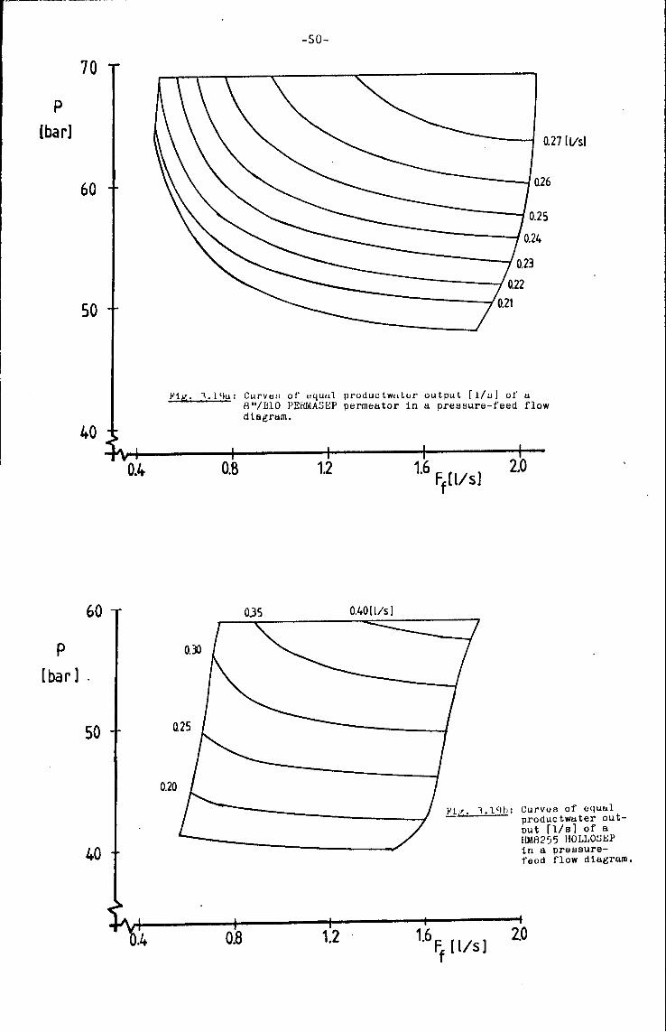
p

[bar]

p

[bar 1

70

60

50

40

0.4

60

50

40

-50-

0.27 IVsl

0.26

~'ig. l.llJu: Curvtw of' uquul productwutur output [1/u] of a A "/BlO PERMA~l!:P permtHi tor in a pressure-feed flow diagram.

0.8 1.2

0.35

0.20

0.8 1.2

0.40[1/sl

2.0

Curvos of oquul productwater out­put n/sl of a IIMA255 HOLLO~l!:P in a pressure­feod flow diagram.

2.0

p

[bar)

p

[bar]

70

60

50

40

60

50

40

0.4

0.4

-51-

4(kWJ 5 6 s 10 12

r'ig. ·l.?Oa: Curv~:~s of ~:~qutd net pow~:~r· requirem~:~nt [kW] of a 8 "/BlO PEHMASEP pormea tor in a pressure-feed flow diugrum.

0.8 1.2

6 7 e

0.8 1.2

9 10ikW]

;;..=;;~l~·=20;..:;;b: Curves of equal net power require­m~:~n t [kW] of a HMR?55 HOLLOSEP

1.6 [ ~ l/s]

2.0

in H pressure­feed flow diagram.

p

(bar]

p

[bar]

70

60

50

40

60

50

40

0.4

0.4

-52-

10

J.'ig. 1. ?lu: CurvtHJ of equul ne t 1energy con!lumption per amount of produc twli ter [ kWh/m ) of li A"/ BlO PEHMASEP permali tor in a pressure-feed flow di~:tgram,

0.8 1.2

0.8 1.2

1.6 Ff [ l/s 1 2.0

;_!;.1.:..:.,__...:..1:..:.. ?....::l.:;;b: Curve a of equal

1.6 [ ] ~ l/s

2.0

net tJnergy con­sumption per amount of pro~uctwater [kWh/m ] of a HM8?55 HOLLOSEP in u pressure-feed flow diagram.

p (bar)

p [bar]

70

60

50

40

0.4

60

50

40

-53-

300 ppm

350

Fig. l.??a: Curves of equal salt concentratien [ppm) in the productwater of a A"/BlO PEHMASEP permeator in u pressur~-feed flow diagrum.

400

45() ..

500

0.8

250

0.8

1.2

200 ppm

1.2

1.6 F 2.0 f ll/s)

l.??b: Curves of equal .:.-:..~;..;....~~ Btil t conct:Jntr~:~.tion

1.6 ~ [ l/s)

[ppm] in the productwater of a HM8?55 HOLLOSEP in a pressure­fe~ct flow diagram.

2.0

70

p

[bar)

p

[bar]

60

50

40

60

50

40

0.4

-54-

024 Q20 0.16 0.14

r'11:(. ·1.?11.1: Curvrw of equt1l convurR1on of a A"/rno PimMASEP pormou Lor ln 1:1. pro :J:Juru -t'ouu f luw u lugrwu,

0.8 1.2

0.40 0.36 032 0.28

08 1.2

1.6 [ Ff lis]

2.0

0.24

.;..-...~..:..1-.. ?.....;1-.b: Curves of equal convt:lrsion of a HMA255 HOLLOSEP in a pressure­feed flow diagram.

1.6 [ 2.0 Ff lis J

-55-

4. THE FEASIBLILITY OF WIND-POWERED REVERSE OSMOSIS PLANTS

4.1 Introductory remarks

For the determination of the feasibility of wind-powered RO-plants it is essential to match the characteristics of the RO-plant and the windturbine in a_proper manner.

Usually an RO-plant is driven by a constant power supply (diesel genera­tor set in case of smalland medium plants). A windturbine introduces the aspect. of a varying power supply to the RO-plant, assuming long term starage is not applicable and back-up (e.g. an existing grid) is not pos­sible.

Three possible configurations of windpowered RO-plants (windpower only) have been considered: 1) The RO-plant is driven at constant conditions.

If the windturbine delivers sufficient power, i.e. the rated power requirement of the RO-plant, it is coupled to the RO-plant and continues to deliver the same power output even at higher windspeeds. Section 4.3 deals with this configuration.

2) The RO-plant is driven at varying operating conditions dependent on the windspeed. In this configuration one makes use of the capacity adapting ability of the membrane modules as shown in section 3.6. The windturbine is coupled to the RO-plant when its power output is sufficient to drive it at its minimum power requirement. At higher windspeeds the RO-plant is expected to be controlled so as to not exceed operation limits of the RO-modules. This will be further developed in section 4.4.

3) Switching of the membrane area. Each membrane module is operated at constant conditions which can be chosen optimally and as the windturbine output varies the number of operating membranes varies. This configuration will be discussed in section 4.5.

For each configuration it is possible to give energy output (and water production) estimates as a function of the design parameters of the wind­turbine. This is based on the use of Weibull windspeed distributions. The principle of the calculations will be outlined in this section. The reader is referred to appendix E and [55] for more detailed information.

The performance of a Wind-Energy Conversion System (WECS), which includes rotor, transmission and laad, can be expressed by its power output curve (figure 4.1) which gives the power output as a function of the windspeed.

' I

/" I DEAL OUTPUT

------------- ;----------. I

~ig. 4.1: Power output of a WECS.

-56-

The windturbine starts to deliver power at cut-in windspeed v • At windspeeds c above the rated windspeed v the power output is limited e.g. by means of a

r aerodynamic control and above the furlin·g windspeed v f the windturbine is

shut down. The shape of the power output curve between v and v is depen-e r denton the nature of the WECS (e.g. electricity generation, waterpumping). The power output of a WECS can be represented by:

3 P = (c n)l/2pAv p

where: P = power output [W] c = power coefficient p

n = efficiency of transmission, hearings, generator etc. v = windspeed [m/s] A = rotor area 3 p = airdensity [kg/m']

The windturbine reaches its highest efficiency (c ) at the design p max

windspeed vd. The dashed line in figure 4.1 represents an ideal windturbine

(which runs always at its maximum efficiency). The Weibull distribution appears to be very useful in the description of windregimes [56]. lts probability density function can be expressed by:

(4 .1)

f(v) = ~ c!)k-lexp{ -(!)k} (4.2) c c c

where: v = windspeed k = shape factor c = scale parameter = v/r(l+l/k)

00 (v= 0J vf(v)dv = average windspeed; r = gamma function)

This probability density function is depicted in figure 4.2 for several values of the shape factor k.

1.4 r-------,,-------,----.----,----r----r-----,

0.2

0 0 2 3

fig. 4.2: Weibull probability density function for several va1 ~u)es of the shapefactor as a function of the dimensionless windspeed x (=v v

-57-

Energy output estimation can easily be executed by means of:

"" E = T f P(v)f(v)dv 0

where P(v) represents the power output curve. For example, for T=8760 hours E represents the annual energy It appears that for a given shape of the P(v)-curve equation be written ·as:

output. 4.3 can

where e is called the dimensionless energy output [57] which is a syst

(4. 3)

(4 .4)

function of the design parameters x ,x and xf and the shapefactor (windregime), c r x Is the dimensionless windspeed (x=v/V). Thus the energy output is a function of the rotor area, the windregime and the design of the WECS.

In a desalination plant the waterproduction is subject tö economical optimisation. In section 4.3-4.5, descrihing the aforementioned configura~ tions of windpowered RO-plants, the two most important variables for the economical optimisation viz. the rotor area A and the installed RO-capacity CRO will be calculated for several windturbine designs based on a certain

annual waterproduction Wp. The resulting watercasts which will be calculated

in section 4.6 will be compared with the water casts of an RO-plant with a common energy supply. For small autonomously operated plants this is usually a diesel generator set. First we shall consider this so-called base case in section 4.2.

4.2 The base case: operation with a diesel generator set

In the base case the RO-plant is powered by a diesel generator set. The plant scheme is depicted in figure 4,3,

FOSSIL

FUEL

DIESEL GENERATOR

SET

(energy conversion efficiency = 0.25)

ELECTRICAL ENERGY RO-MODULES

PRETREATED

FEEDWATER HIGH

PRESSURE PUMP

(efficiency=0.75)

tig. 4,3: Scheme of a diesel-powered RO-plant.

...... ...... ...... .............

VALVE

BRINE

PRODUCT WATER

-58-

The waterproduction rate is equal to F (m3/s) (which is equal to the p

installed capacity CRO ) at an energy consumption of E per amount of . net productwater which is chosen as low as possible within the operating limits. The actual energy consumption will be higher because of: 1) the pump efficiency which is set equal to 0.75 2) auxiliary equipment like feed pumps, chemica! dosage pumps, controls etc ..

This increases the energy consumption with approximately 10%, The net power requirement(RO-modules only) is equal to:

3 where: Ff = flow of feedwater [m /s] 3 F = flow of productwater [m /s]

Ene~ = net energy consumption per amount of productwater [J/m3]

pf = feedwater pressure relative to ambient pressure [N/m2]

The energy consumption per amount of productwater is equal bo:

Plf pf E = - = (equation 3.16) net F y-

p

where Y is the conversion.

The first departure from the base case concerns the introduetion of an energy-recovery system.

FOSSIL DIESEL GENERATOR

FUEL SET

RO-MODULES I', PRODUCT

PRETREATED' ~

.... WATER ..... ... .... - .... ...... - - ... Ff

.... ..... Fp -FEEDWATER' ...............

-

ENERGY -RECOVERY -- I

BRINE

•• fig. 4,4: Scheme of a diesel-powered RO-plant witr. energy recovery.

(4. 7)

--

-59-

For the net power requirement of an RO-plant with energy recovery one can write:

PRO= pfFf- nerpfFb = pfFf(l - ner(l-Y))

where:Fb = brine flow rate [m3/s]

ner= the total efficiency of the energy recovery system, i.e. the efficiency of the energy recovery system and a correction for the loss in hydraulic pressure in the membranes ( in standard test conditions about 5% [52]1

(4. 8)

From [26] it follows that the maximum value of n is equal to about 2/3. With help from (4.8) we can derive an expressionerfor the energy consumption per amount of productwater in case of energy recovery:

F p

= Pf (1 - n (1-Y)) Y er

(4 .9)

From equations 4.8 and 4.9 one can see that the correction factor for the net energy consumption per amount of productwater (1-n (1-Y)) (and likewise er for the net power requirement) is a linear function of the conversion Y.

CORRECTION FACTOR 1-Tler(1-Y)

1--------

0+-------------------~--CONVERSION 1

fig. 4.5: Correction factor for the net power requirement and the net energy consumption per amount of productwater in case of energy recovery.

4,3 Wind-powered reverse osmosis plant operating at constant conditions

In this configuration it is assumed that the windturbine drives the RO­plant at constant conditions. The operating conditinns will be the same as in the latter section, preferably leading to the most energy-efficient process, Figure 4.6 depiets the plant scheme of this wind-powered RO-plant.

It is obv1ous that the use of a windturbine as the energy supply results in lower operation times compared to the base case. Enhancement of the waterproduction capacity is necessary to deliver the same annual amount of freshwater as in the base configuration.

..

PRETREATED

FEEDWATER

TRÁl"lSMISSION AND

CONVERSION

-60-

HO-MODULES (constant eperating conditions)

.....

...... .....

....... ......

VALVE

BRINE

PRODUCT

WATER

fig. 4.6: Plant scheme of a wind-powered RO-plant operating at constant conditions.

In figure 4.7 the power output curve of the windturbine in this configuration is depicted. The windturbine is coupled withethe RO-modules if the windspeed exceeds a certain rated value x and is consequently able to cover the net

r power requirement of the RO-modules. The losses of the high pressure pump and the auxiliary equipment will be accounted for, later.

---------

/

/ /

I I

I

I

I

I I

/"" IDEAL OUTPUT

fig. 4.7: Power output curve of a windturbine coupled with an RO-plant operating at constant conditions.

-61-

The power output curve can be written as:

0 if O<v<v or V'L,Vf P(v) { --r

l4.10) = p if v~v~vf wr

Using equation 4,3 the energ~ output of this specific WECS can be determined (see appendix E).

E = e (x ,k)(c n) 1/2pAv3T syst r p max 3 k k where: e (x ,k)= x exp{-r (1+1/k)x } syst r r r if xf is set to oo~

In appendüc: F e (x k). is depicted as a function of x and k. syst r' r

(4.11) can be written as:

E = P Te t(x ,k)/x3

wr sys r r

e t(x ,k)/x3 can be interpreted as the availability of the windturbine sys r r k k

and is equal to exp{-r (1+1/k)x }. r

The annual waterproduction is equal to W with p

W = E/t:. p

(4.11)

(4.12)

(4.13)

where e represents the overall energy consumption per amount of productwater, The required capacity of waterproduction CRO (viz. to produce the required

annua1 amount of W ) is equal to the average waterproduction divided by p

the availabi1ity of the windturbine:

w CRO = p 3- =

Te t(x k)/x sys r, r

1

3 x

r e (x k) syst r'

or C = (C ) RO RO diesel exp(-rk(l+l/k)xk)

r

In figure 4.8 the dimension1ess plant capacity cR0

/(Wp/T) is given as a

function of x for several values of the shapefactor k. r

The rotor area requirement can be determined by substitution of equation 4.11 in equation 4.13. Rewriting gives:

w A = ....E.

1

T .3 e (x k) (c n) 1/2pv syst r' p max w

Calling A f = ....E. -------=-re T .3 (c n) l/2pv p max

rotor area:

A 1

-A-= e (x k) ref syst r'

this can be written as a dimensionless

( 4 .14)

( 4. 15)

-62-

In figure 4.9 the dimensionloss rotor area rcquiromcnt is depicted as a function of x for several values of k. It appears to have a minimum value.

r

---- I . -

8--­

/

DIMENSIONLESS RO-PLANT CAPACITY

1' ---···· k=3.5 I t•' ; •••--· c· • •!

i

----------~---.------- -~----·-r-

'

. I ---·-·------~--- ---·-··

3- I I

/_-- ---------------:----.----------- --,------· -·-

JU- I-

:--_ t~~-:---:---=~~~~~:-~::~ ~---- ~--7- i··

I

I --t-----~r--------r-·----·-----.... - -··-----,-

! ' '

2

0

k=2

k=l.5

t------·

I , ï -------- ___ ,

-·- ---------------+-------< ! I

·-- --- + ·r ... -- ~-

I i

+------,----t----~1 ___ ------+-----1 I

2 xr Î

fig. 4.8: Dimensionless plant capacity (CR0/(Wp/T)) as a function of the

dimensionless rated windspeed x (=v /v) for an RO-plant eperating at constant conditions. r r Note: for the base case (diesel) CR0/(Wp/T)=l.

-63-

10 DIMENSION- r k=3.5 k=2 LESS ROTOR AREA·-·-··

a·

6

4

2

0 0 1 2

fig. 4.9: Dimensionless rotor area (A/Aref) as a function of the dimensionless

rated windspeed x (v /V) for an RO-plant at constant operating r r

conditions.

4.4 Wind-powered reverse osmosis plant operating at varying conditions

It is assumed that the RO-modules are able to withstand a varying power input at constant pressure in this configuration. The plant scheme is given in figure 4.10. The windturbine is coupled with the RO-plant if the windspeed exceeds a certain cut-in windspeed v , At this windspeed the windturbine is able to drive the RO-plant just atcits minimum power requirements. At windspeeds between v and the rated windspeed v the RO-plant is driven at conditions c r between its minimum and maximurn power requirernent. At windspeeds above the rated windspeed the RO-plant is driven at its maximurn power requirement but still within its operating lirnits.

The matching of an RO-plants and a WECS is in essence the matching of a constant head positive displacement pump with a windturbine (for srnall and medium capacities}. In [57] a model is presented of a windt!'fbine driving a positive displacement pump. It assurnes the average pump~~.;_ ·iLw to be constant and furtherrnore that the relationship between windturbine torque and nurnber of revolutions is linear. The resulting mathematica! expression for the power output is:

3

• TRANSMISSIO

AND CONVERSION

V<V c

-64-

RO-MODULES (varying eperating conditions

...... ..... PRETREATED ......

FEEDWATER • ...... . '1 ...... ...........

PRODUCT

WATER

VALVE

BRINE

fig. 4.10: Plant scheme of a wind-powered RO-plant operating at varying conditions.

0 if 0 < V < V = = c or v.:;: vf

P (v) = { v vd 3 (2- - - ) (c n) l/2p Avd if V < V < V

vd v p max c r

P if V ~V < Vf wr r -

where vd is the design windspeed.

This power output is drawn in figure 4.11.

Setting vf=oo the energy output can be expressed as

E = e t(x ,x ,xd,k)(c n) l/2pAV3r sys c r p max

according to(4.4) (x=v/v).

It must be reminded here that x and x are related by the fact that they c r represent the minimum and maximum power requirement respectively. Assuming the maximum power requirement to be three times the ment (see section 3.5) an expression can be derived of vd and vr:

2 ~ 2 vd vd 2 2 vc = (2vr- v ... (2vr-v) + 72vd )/12

r r

minimum power require­for v in dependenee

c

(4.16)

(4.17)

(4.18)

-65-

I I' IDEAL OUTPUT

L 71-------,

ffuin

fig. 4.11: Power output of a windturbine coupledtoa positive displacement pump.

The dimensionless energy output can now be expressed as: x

•syst (xd,xr,k) = x/ Gk Jl~/ -:d]xk-l e~Gx k dx + xd 3

• [2 ::- ::]. -Gx k

e r

x k c ( 4. 19)

(G=r ·(1+1/k); x (=v /v) is determined with 4.18) c c

The results of the calculations of e t of this configuration are presented in appendix F. sys

The ability of the RO-modules to adapt themselves to varying power input is possible at the expense of a higher energy consumption per amount of productwater and a lower conversion (see section 3.5). Figure 4.12 depiets the range of energy consumptions per amount of productwater for several operating conditions in a energy consumption-power input diagram (8"/BlO PERMASEP permeators). For the PERMASEP permeator the minimum vales of the energy consumption per amount of productwater {corresponding with a maximal productwater output) coincide with the operation at maximum pressure and show a linear dependenee on the power input. For the HOLLOSEP this is not quite the case. For the latter membranes the pressure has to be lowered in order to reach the low values of the net power requirement and consequently the productwater output decreases. The waterproduction rate can be expressed as:

P/E:

where: ·p = the supplied power e = the energy consumption per amount of productwater

Then the annual waterproduction can be written as:

(4. 20)

NET 14 ENERGY

CONSUMP,ION [kWh/m ] 12

10

8

6

4

2 / /

/

/ /

2 4 6

-66-

8 NET

/ /

10 12 14 POWER [kW]

fig. 4.12: Range of energy consumption per amount of productwater (E) at several operating conditions for a 8"/BlO PERMASEP permeator. (determined from figure 3,20a and 3.2la)

In words: the annual waterproduction is dependent on the windturbine design (x , x, xd),

c r rotor area A, windregime (k,v), RO-plant characteristics and the control strategy (E (P)) .

In order to get an idea of the feasibi1ity we assume that at any power input the RO-modu1es wi11 operate at their lowest energy consumption per amount of productwater. According to figure 4.12 the dependenee of E on the power input wi11 be linear. This relationship is 'depicted in general terms in figure 4.13(the rated windpower P is equa1 to P =3P . (figure 4.11)). wr max m1n

E can be

E = E . m1n

or

written as: p - p .

m1n ""p--_-p=---.- (Emax - Emin)

max m1n +

p - p /3 wr

E = E . + 2P /3 (Emax - Emin) ffi1n wr

Substituting equation 4.21 in equation 4.20 we get:

00

W = T /----..--=P_(::..,v,.:.) ----- f (v) dv p o· p - P /3 wr

Emin + -:::-2-;:::P-/"7':='3-- (Emax - Emin) wr

(4.2la)

(4.2lb)

(4.22a)

net energy

consumotien

-67-

Pmax (Pwr)

net power

fig. 4.13: Hinima1 energy consumption per amount of productwater in dependenee on the RO-p1ant power input.

or: 3 00

(c n) 1/2pAv j W = p max ·T. P e: . m1n

P(x) e: - e: . P(x) P(x )/3 f(x)dx max m1n ( r )

e: . 2P(x )/3 m1n r 1 +

in which p (x) represents the dimensionless power output:

0 if 0 ~x~x or x > x c = f

P(x) { x xd 3 if x = (2-- -)·x < x < x

xd x d c r

x xd 3 r P(x ) if (2- - -)·x = x < x < xf xd x d r r=

r

Denoting the integra1 in (4.22b) as wsyst we can write for the rotor area requirement:

w e: . 1 _.E. m1n

A= r ·cc n) 1/2pv3-· w p max syst

or:

A 1 A ref

= w syst

(4.22b)

(4.23)

-68-

In figure 4.14 the dimensionless rotor area requirements are depicted as a function of the dimensionless design windspeed for several values of the dimensionless rated windspeed and several shapefactors k. From figure 4.12 the value of CE -E . )/E . is estimated to be l.S. max m1n m1n It appears that the dimensionless rotor area has certain xd for constant xr. Also for constant xd

a minimum value at a x has a minimum value. r

The plant capacity CRO can analogous to C4.7) determined from:

CRO = P . /E . =CP /3)/E . m1n m1n wr m1n

With P = wr

this can be

xr xd 3 3 {2- - -) xd · (c n) l/2pAv

xd xr p max

written .as:

W 1 x xd 3 1 C = Î. -C2_!_- -)x·--

RO T 3 xd xr d wsyst

(W /T is equal to CC ) ) p RO diesel

and the expression forA C4.23)

The dimensionless plant capacity CR0/CWP/T) is depicted in figure 4.15 as

a function of the dimensionless design windspeed xd for several values of

the dimensionless rated windspeed x for several shapefactors. From the figure we see that for the considered values of the design parameters an increasing value of xr or xd results in an increasing RO-plant capacity.

c 4. 24)

( 4. 25)

10 DIMENSION­LESS ROTOR AREA

9

8

7

6

5

4

3

2

1

0

-69-

1.e

k=1.5

0 1

1.2 1.4 1.6 1.8

2

2.0

2.2

2.4 3.0

3

fig. 4.14a: Dirnensionless rotor area (A/Aref) as a function of the dirnensionless

design windspeed xd for several values of the dirnensionless rated

windspeed x and for k=l.S. r

10 DIMENSION­LESS ROTOR AREA

9

8

7

6

5

4

3

2

1

0 0

-70-

2.0

2.4

k=2

1 2 fig. 4.14b: Dimensionless rotor area (A/Aref) as a function of the dimensionless

design windspeed xd for several values of the dimensionless rated

windspeed x and for k=2. Note:For vaiues of x > 2.4 the dimensionless larger than the graph for xr=2.4. Graphs for are not drawn.

rotor area will be these vàlues of x

r

3

10 DIMENSION­LESS ROTOR AREA

9

8

7

6

5

4

3

2

1

0

-71-

xr =O.R 1.0 1.? 1.4 1.6 l.R

k=1.5

0 1 2 .3

fig. 4.14c: Dimensionless rotor area (A/Aref) as a function of the dimensionless

design windspeed xd for several values of the dimensionless rated

windspeed and for k = 3.5. Note: For values of x > 1.8 the dimension1ess rotor area wi11 he

r larger than the graph for x =1.8. Graphs for these va1ues of x r r

are not drawn.

3

2

1

0 0

DIMENSIONLESS HO-PLANT CAPACITY

xr = 1.0

2.R

2.6

2.4 ?.2

k=l.5

0.4

-72-

0.6 0.8 1.0 1.2 1.4 1.6

fig. 4 .!Sa: Dimensionless lW-plant capacity (CR0; (Wp/T)) as a function of the

dimensionless design windspeed xd for several values of the dimension­

less rated windspeed x and for k=l.S. r

(CR0/(Wp/T) = 1 for base case (diesel)).

3 DIMENSIONLESS

0 0

RO-PLANT CAPACITY

k=2

0.4 0.6

-73-

0.8 1.0 1.2 1.4 1.6 fig. 4.15b: Dimensionless RO-plant capacity (CR0/(Wp/T)) as a function of the

dimensionless design windspeed xd for several values of the dimension­

less rated windspeed x and for k=2. r

(CR0/{Wp/T) = 1 for base case (diesel)).

3

2

1

0 0

DIMENSIONLESS RO-PLANT CAPACITY

x = r 3.0-__,

2. 4-----.r' 2 • 2 _ ___"_.,

k=3.5

OJ.a.

-74-

0.6 0.8 1.0 1.2 1.4 1.6

fig. 4.1Sc: Dimensionless RO-plant capacity (CR0/(Wp/T)) as a function of the

dimensionless design windspeed xd for several values of the dimension­

less rated windspeed x and for k=3.5. r

(CR0/(Wp/T) = 1 for base case (diesel))

-75-

4.5 Wind-powered reverse osmosis plant operating with varying membrane area

The plant schemeof the last wind-powered RO-plant to be discussed is given in figure 4.16.

..

..

PRETREA TE FEEDWATER

TRANSMISSION AND

CONVERSION

V<.V c v~v0

HO-MODULES

fig. 4,16 Plant scheme of wind-powered RO-plant operating with varying membrane area.

The windturbine is coupled to the RO-modules if thc power output is sufficient to operate the first RO-module. If the power output increases the next module may be swithed one etc. The windturbine output is limited if the windspeed exceeds a certain rated windspeed v (e.g. by means of an aerodynamic control) The resulting power output is giveft in figure 4.17

A real RO-plant will consist of a series of RO-modules which can be switched on/off. For the ease of calculation it is assumed that the membrane area can be varied continuously along the third power curve (fat curve in figure 4.17). The power output can bedescribed by:

0 if 0 < V < V = c or v .:::._ v f

P(v) == { 3

(c Tl) l/2pAv if V < V < V p max c r

P wr i f v r ~ v < v f

The annual energy output of this ideal WECS can be written as (xf==oo):

(4. 27)

fTnïn

-76-

I

I I

I

fig. 4.17: Power output of a windturbine which drives an RO-plant with varying membrane area.

E = e (x ,x ,k) (c n) l/2pAv3

syst c r p max Xr

wnere: e (x ,x ,k) syst c r , G {xk+2 -G xk dx 3 Gx k

e +.x.e r r .

(G=fk (1 + 1/k))

e (x x k) Is depicted in appendix F as a function of x for several syst c' r' r

values of the shapefactor k and . x =0. c

If we assume that each RO-module will be operated at the condition of the lowest energy consumption per amount of productwater (s) the annual water­production can be written as:

W = E/s p

Using this an expression for the installed capac~ty CRO can be derived

with help from equations (4.27) and (4.28):

w = p

e P syst ~

3 ~

e = CRO syst 3

(according to (4.7)

x x r r

or

W x3 x3

= _.E. r = (C ) r T -e---- RO diesel e t

syst sys

The dimensionles~ RO-plant capacity is equal to: x r

CRO/ (W /T) = -e--p syst

( 4. 28)

(4.29)

(4. 30)

-77-

The dimensionless plant capacity which is an increasing function of the dimensionless rated windspeed x is depicted in figure 4.18 for several

r values of the shape factor k. Cxc =0).

JU·-i--·-··· cl -- '---------·· ·-----

b- DIMENSIONLESS 1 . RO-PLANT

.L '- -- -- ·-·· -1

: CAPACITY c., . r------:-----~---·-·-·----

1 'J-· . 1---· ·-

1

4· ·r- ----

I "J--1----·---: ___ _

I ,

I I I ,I

l. ---~----·-·--- --- ---·-----------· -------·. ----· --- ----

-'

2·· -- ·------·- ---·-·------ --- ----·- ---·-·-;-·

. - ---------- - ---- ----1-

0 1 2

/

k=3.5

k=2

'

·-- --/< /J _/"'- .,.

/ k=l.5

··t·-----

. ' ' '

r-i

--1-·----

' 1-!

i : i ·-'·-- ·---- _ _. ________ , _____ ----r---1

' ' ' I , I ) X , I

r -----

fig. 4.18: Dimensionless RO-plant capacity (CRO/(Wp/T)) as a function of

the dimensionless rated windspeed x for several k-values, r

(CR0/(Wp/T)=l for the base case (diesel)).

I

-78-

The rotor area requirements can be derived with equations 4.28 and 4.29: w

A = _J?.. e: =-:s- --=-1-----..--T (c n) 1/2pv- e t (x ,x ,k) ( 4. 31)

p max sys c r

w Setting Î e: -3- = A

T (c n) l/2pV ref p max this can be written dimensionless1y:

A 1 ( 4. 32)

The dimension1ess rotor area requirement is depicted in figure 4.19 as a function of the dimensionless rated windspeed x for several values of the shapefactor k (x =0). r

c The dimensionless rotor area is a decreasing function of x which goes

r asymptotically to a minimum value.

6 DIMENSION­LESS ROTOR i\ REA

5

4

3

1

0

k=l.5

0 1 2

k=3.5

fig. 4.19: Dimension1ess rotor area (A/A f) as a function of the dimension1ess rated windspeed x for scvcraie k-valucs.

r

3

-79-

4.6 Some economie considerations*

In this section waterprices are calculated for each configuration (2 diesel-powered RO-plants and 3 wind-powered RO-plants). The economie calculations are carried out for a situation of an average water demand of 100 m3 per day during 340 days a year. First we shall determine the water casts per m3 for the two diesel-powered plants and then secondly the water casts for the wind-powered plants in which the windturbine will be a parameter for the economie optimisation, The economie parameters for an RO-plant are listed in table 4.1.

table 4.1: Economie parameters of an RO-plant consisting of BlO PERMASEP permeators [61].

Investment casts

Maintenance Chemieals Operating casts Interest rate

Dfl 5000.-- per m3/day consisting of: - 40% membranes (5 years lifetime) - 60% plant (15 years lifetime) 2% of investment per year Dfl 5000.-- fora 100 m3/day plant per year labor (p.m.) 10%

The annual casts resulting from an investment at the beginning of a period of N years can be deterrlined by mul tiplying the investments by the so-called capita! recovery factor which is equal to:

.T in which r represents the inter~st rate corrected for inflation.

1 - (l+r)-N

Table 4.2 represents the economie parameters of the diesel generator set.

3 + table 4.2: Economie parameters of a diesel generator set for 100 m /day plant.

Investment costs (30kW-50kW): Dfl 35000.--Lifetime 10 years ~~intenance 5% of investment casts per year Energy efficiency (fuel to electrical energy) Diesel fuel casts Interest rate

25% (1 litre diesel~2.5 kWh) Dfl 1.-- per litre 10%

+ Based on manufacturer's information. These values seem rather optimistic. _Existing diesel generators appear to have shorter lifetimes and maintenance costs which can be as high as 30% of the fuel costs.

The operating conditions of the RO-plant are listed in table 4.3.

* 1 US$~ Dfl 3.- (three dutch guilders), march 1984.

-80-

table 4.3: Operating data of the RO-plant consisting of BlO PERMASEP permeators.

Pressure Conversion Net energy consumption per amount of productwater Pump-efficiency Auxiliary energy consumption:

69 bar 40%

3 4.8 kWh/m (see section 3.5) 75% 10% of net energy consumption

From the data presented in table 4.3 the gross energy consumption per amount of product is estimated to be 7.2 kWh/m 3 •

The waterprice which èan be calculated from these data is equal to 3 Dfl 6.25 per m (46% fuel casts)

Most economie parameters wil! be the same as in the preceding case except for an additional investment of Dfl 10000,-- for the energy recovery system. According to equation 4.9 with n =2/3 and Y=0.4 the energy consumption per

er ~ amount of productwater will be equal to 0.6•7.2=4.32 kWh/m . The resulting waterprice is equal to

Dfl 5.12 per m3 (34% fuel casts)

In the following the waterprices in case of wind-powered plants will be calculated. Table 4.4 presents the economie data for the windturbine(s).

table 4.4: Economie parameters for windturbines.

fnvestment casts Lifetime Maintenance + insurance Interest rate

2 Dfl 1000.-- perm of rotorarea 15 years 2.5% of investment casts per year 10%

The proposed windturbinecasts are somewhat higher than the current casts for electricity producing windturbines [62] to account for the additional casts of controls. These extra casts are assumed to be the same regardless of the chosen configuration. For each of the configurations expressions have been developed for the required plant capacity-and the required rotor area in dependenee on the design parameters of the windturbine (x ,x ,xd). c r The calculations have been carried out for three k-values (1.5,2,3.5) and a mean windspeed of 8 m/s. Furthermore, (c n) =0.32, p=l.2 kg/m 3 ,.

3 p max

E=E . = 7.2 kWh/m and the casts of chemieals are assumed to be the same m1n

as in the diesel configurations.

~~~~:E~~~E~~-~9:E~~~!~-~!-~~~~!~~!-~E~E~!~~g-~~~~~!~~~~

With equations 4.14 and 4.15 respectively the required RO-plant capacity and the required rotor area are determined. These are the inputs for the economie calculations. The resulting waterprices are presented in figure 4.20 as a function of the dimensionless rated windspeed x . r

WATERPRICE [fl/m3]

15 14 13 12 11 10

9 ·8

-81-

k=3. 5---i k=l.5

7 6

DIRSEL-POWERED. WITHOUT ENERGY~RECOYERY

DIESEL-POWERED WITH ENERGY-RECOVERY 5

0 1 2

fig. 4.20: Calculated waterprices of a wind-powered RO-plant operating at constant condi ti ons (v=8m/ s; e:=7. 2kWh/m3) See tables for t:1e economical parameters.

Table 4.5 presents the minimum waterprices and their compostion for several shape factors.

Table 4.5: Minimum waterprices for the RO-plant operating at constant conditions.

k . 1.5 2 3.5

Waterprice (Dfl/m3) 10.20 9.40 8.10

Energy fraction 38% 38% 38%

RO-plant fraction 60% 60gó 60%

Chemieals fraction 2% 2% 2%

-82-

With equations 4.23 and 4.25 respectively the required rotor area and the required RO-plant capacity are calculated. Next the waterprices can be determined These are depicted in figure 4.21 as a function of the dimension­less design windspeed xd for several values of the dimensionless rated wind-

speed and the shapefactor k.

WATERPRICE [fl/m3]

15 14 13 12 11 10

l.R

k=l.5 9 8 7 6 5

DIESEL-POWEHED WITHOUT ENEHGY-RE00VEHY

fig. 4. 21a:

DIESEL-POWEHED WITH ENERGY-RECOVERY

0 1 2 Waterprices for a wind-powered RO-plant at varving operating conditions as a function of the dimensionless design windspeed for several values of the dimensionless rated windspeed (k=l.S;v=8m/s;E . =7.2 kWh/m 3). See tables for the . 1 m1n econom1ca parameters.

Table 4.6 presents the minimum waterprices and their composition for several shapefactors.

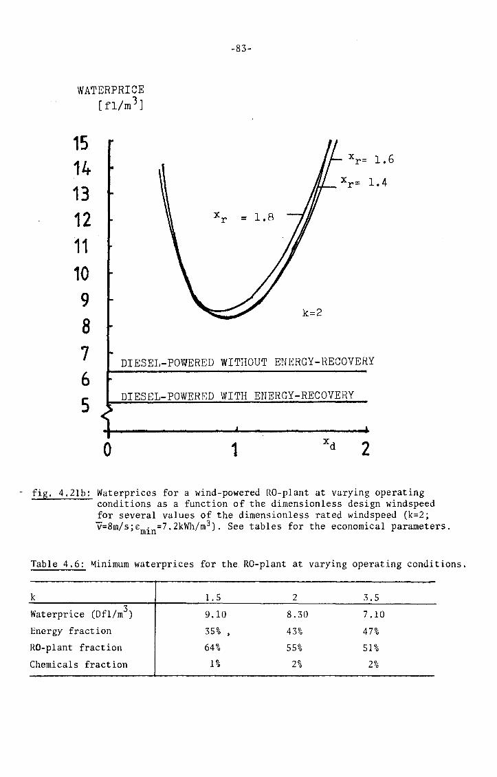
WATERPRICE [fl/m)]

15 14 13 12 11 10

-83-

9 8 7 6 5

DIESEL-POWERED WITHOUT ENERGY-RECOVERY

DIESEL-POWERED WITH ENERGY-RECOVERY

0 1 2

- fig. 4.2lb: Waterprices for a wind-powered rW-plant at varying operating conditions as a function of the dimensionless design windspeed for several values of the dimensionless rated windspeed (k=2; v=8m/s;€min=7.2kWh/m 3). See tables for the economical parameters.

Table 4.6: Minimum waterprices for the RO-plant at varying operating conditions.

k l.S 2 3.S

Waterprice (Dfl/m3) 9.10 8.30 7.10

Energy fraction 3S% 43% 47%

RO-plant fraction 64% SS% Sl%

Chemieals fraction a 2% 2%

-84-

WATERPRICE

15 14 13 12 11 10 9 8 7 6

5

fig. 4.2lc:

[fl/m3 ]

xr.= l.?

k=3.5

DIESEL-POWEltED WITHOUT ENEHGY-HECOVEHY

0 1 . 2

Waterprices for a windpowered RO-plant at varying operating conditions as a function of the dimensionless design windspeed for several values of the dimensionless rated windspeed (k=3.5; v=8m/s;E . =7.2kWh/m 3). See tablesfor the economical parameters.

m1n

With equations 4.30 and 4.31 respectively the required RO-plant capacity and the required rotor area are determined. These results are the inputs for the economie calculations. The resulting waterprices are depicted in figure 4.22 as a function of the dimensionless rated windspeed x .

r Table 4. 7 presents the miiümum waterprices and their composition for several shapefactors k.

15 14 13 12

11 10 9 8 7 6 5

0

WATERPRICE [fl/m3]

-85-

k=J.5---I

DIESEL-POWERED WITHOUT ENEHGY-RECOVERY

DIESEL-POWERED WITH ENERGY-RECOVERY

1 2

fig. 4.22: Calculated waterprices for a wind-powered RU-plant witn varying membrane area, (v=8m/s;E=7.2kWh/m3). See tables for the economical parameters,

table 4.7: Minimum waterprices for the RO-plant operating with varying membrane area.

k 1.5 2 3.5

Waterprice (Dfl/m3) 7.80 7.00 6.10

Energy fraction 32gó 3!9ó 31 gó

RO-plant fraction 67% 67% 67%

Chemieals fraction 1% 2% 2%

-86-

Discussion

We can summarize the results of the calculations for these speci.C:ic circum­stances (v=8m/s;E=7.2kWh/m3 ;100m3/day-plant): 1) Lowest waterprices occur at high k-values. 2) The wind-powered RO-plant with continuously varying membrane area gives

rise to the lowest waterprice i.e. of the three wind-powered configurations. Second lowest waterprices result from the RO-plant with varying operating conditions and the highest waterprices result in the RO-plant is operated at constant conditions.

3) The comparison of the composition of the minimal waterprices shows that the windpowered RO-plants operating at constant conditions or with vary­ing membrane area have a composition which is fairly insensitive to the value of the shapefactor k, the RO-plant fraction being somew~at larger in the RO-plant with varying membrane area. This is quite different for the wind-powered RO-plant operating at varying conditions. In this configuration the narrow shape of the probablility density function (figure 4.2) at high shapefactors (k~3.5) offers a better fit to the allowable power range of thc lW-modules (J> =3J> . ) . This results in max m1n a lower RO-plant fraction in the waterprice at high shapefactors.

4) Diesel operation without energy recovery gives rise to lower waterprices compared to the wind-·powered plants. Only the configuration of continuous­ly varying membrane area (which is in fact an idealised approximation) gives a somewhat lower waterprice at its optima! design for k=3.5. The lower feasibility is caused by the lower availibility of the wind­turbine (as compared to the diesel), resulting in almost all cases in an increase of the required RO-plant capacity. As the RO-investments are high the influence in the waterprice will be large. The increase in the RO-plant costs has to be compensated for by a decrease of the energy costs which, according to the results, is only possible in one of the cases considered. Diesel operatien with energy recovery renders the overall lowest water­price.

These conclusions are valid for the special situation based on average sea­water (34500 ppm) and all the aforementioned economical parameters. We shall now discuss the applicability of the results: 1) Other seawater concentrations will not influence the results of the

comparison to a large extent except for the configuration with the varying operating conditions. Higher feedwater concentrations decrease the allowable power input variation and thus lower the economical feasibility.

2) In general the waterprices decrease in case of a higher plant capacity. The RO-plants with their modular builcl-up show a modest decrease in investment casts per unit of installed capacity. So do the windturbine casts but to a lesser degree. Thus the economical feasibility of wind­powered RO-plants at capacities >!00 m3/day compared to diesel-powered plants decreases. Furthermore, it can be expected that the energy con­version efficiency in diesel-operated plants may increase in case of larger diesel generators

3) At lower capacities (<100 m3/day) a diesel generator set may not be available for the power supply. Then the power has to be supplied by a motor which runs at a lower energy conversion efficiency. Because windturbine casts increase very little (per unit of· rotor area) it could become an economical alternative to operate RO-plants by wind­turbines. Of course as a ·whole the waterprice would increase at lower capacities.

-87-

4) The results of the comparison between diesel-powered and wind-powered RO-plants are also applicable to other membranes since e.g. the Toyoho membranes show a behavior similar to the Dupont membranes

5) In many far-away places diesel prices can be much higher (up to Dfl 3.-­per litre) and also maintenance costs. Also the assumption of a diesel having a life-time of 10 years is debatable if the diesel operates full­time. This means that in other conditions than supposed wind-energy could be a good alternative to that generated by a diesel set: On the other hand it should be noted that the chosen windregime is very favorable.

Although the given comparison of waterprices is meant as a realistic example, in real situations, however, calculations on the basis of local conditions and economie data should be made.

-88-

5. AUTONOtv!OUS WIND-DIESEL SYSTEMS (AWDS)

5.1 Introduetion

At preseut autonomous wind-diesel systems are being developed and tested throughout the world. An autonomous system is a power plant which can cover a power demand without the assistance of a utility grid. An AWDS is a hybrid wind-fuel power plant in which the installed windpower is larger or of the same order as the installed fuelpower. In [58] a summary of autonomous systems under development is given. We shall focus the attention on the system which is currently being developed at the Eindhoven University of Technology under auspices of CWD (Consultancy services Windenergy Developing countries) and the Dutch windenergy research programme. A block diagram of this system is given in figure 5.1. ·

voltage control

dW Pd. ·lw-lesel dt

diesel

control

frequency control

fig. 5.1: Block diagram of the Eindhoven AWDS.

This AWDS is able to cover a varying power demand. The power balance of this configuration is:

dw pdiesel + Pwind = pextra + pload + Iwdt

where: P diesel = power supplied by the diesel engine

~xtra -(

p . d w1.n = power supplied by the AC/DC/AC converter

pload p extra

= power t:eeded by the autonomous grid

= power fed into the additional laad

autonomous grid

I = moment of inertia of the synchronous machine SM2 and all other connected loads

w = angular velocity of the synchronous machine Sf\12

(5.1)

-89-

When P . d>P1 d the diesel engine can be disconnected frorn its generator w1n oa by rneans of a clutch and is switched off. The synchronous machine SM2 is essential to rnaintain tf,e voltage (and to supply the reactive power) and with help of the controllable load the frequency of the grid is kept constant, The surplus power is fed into the additional load. When P . d<P

1 ·d the diesel engine and the windturbine are in parallel

w1n oa operation, the diesel engine supplying the deficit power. The frequency is rnaintained by the speed control of the diesel engine,

If the load consists of an RO-plant only the power dernand will be constant, In tirnes of calrn the diesel engine has to be able to operate the RO-plant. So.the rated diesel power Pdr is equal to the RO-plant power dernand PRO'

The rated windpower P rnay have values between zero and a value sornewhat wr higher than Pdr' This can be understood by the fact that the diesel engine

consurnes fuel at zero output to keep the synchronous machine and the engine stand-by, These zero-losses rnay also be supplied by the windturbine. There­fore the rated windpower rnay be larger than the rated Jieselpower. Research on the technica! feasibility is at present carried out,

In the following we want to discuss a disturbing feature of AWDS's (or in general of windturbines). Figure 5.2 represents a graphof the power fluctuations duringa ten minute period (59].

Pmur----r----------------------------~

f+f:jl-~--:r.r-~-A------.._---A~II--/conaumers lo«< power

tlmtnl-

)/~~ windpower used by the consurners

ever ~ge wind power INind power

~ excess of windpower, fed into the extra controllable load

fig. 5.2: Illustration of the power fluctuations of a windturbine in an AWDS.

It shows clips and peaks. Excess power (>power dernand) is fed into the controllable load; Deficit power is supplied by the diesel generator. The guaranteed power (Prnin in figure 5.2) is about 1/3 of the average windpower of one windturbine.

There are several possibilities to enhance this value e.g. by the use of more windturbines, by battery starage or by the use of flywheels.

One of the disadvantages of the system as depicted in figure 5.1 is the fact that if the diesel generator set is operated at lower power outputs than its rated power the energy conversion efficiency will increase. To avoid this problern one could ernploy a systern which has two possible operating modes viz. either the RO-plant is operated by the diesel engine or ·by the windturbine. In order to prevent nurnerous start-ups and shut-downs of the diesel engine in this so-called on/off systern attention must be paid to the problern of the windfluctations. Furtherrnore the effective output is expected to be less than that of the Eindhoven AWDS.

-90-

5.2 Fuel savings prediction of an AWDS-powered RO-plant .. The use of autonomous wind-diesel systems instead of windturbines only

has two advantages: 1) The RO-plant can be operated at its optima! conditions. 2) The effective time of operation can be made as high as possible, i.e

no excess plant capacity has to be installed. In order to operate the AWDS economically the fuel costs decrease has to be larger than the extra investment costs due to the windturbine(s) and the controls. First the estimated fuel savings of the Eindhoven AWDS will be determined.

Eindhoven AWDS

It is assumed that the fuel consumption FC of the diesel generator set is a linear function of the diesel power output Pd. This assumption is basedon measurements reported in[60].

FUEL CONSUMPTION

FCr

~la

FUEL SAVINGS

• DIESEL POWER

fig. 5,3: Fuel consumption of a diesel generator set as a function of the diesel power.

The linear relationship can mathematically be represented by:

The negative values of the diesel power can be interpreted by the fact, that the windturbine covers the zero-losses of the diesel generator. In the model which we will use to estimate the fuel savings it is assumed that the value of the rated windpower P is equal to Pd_+S/a where

wr r Pdr represents the rated dieselpower which is equal to the power demand

of the RO-plant (because of the assumed necessity to operate the RO-plant during periods of calm). Furthermore we can define:

y = P /Pd =(Pd +S/a)/Pd wr r r r (this is a system constant, not a variable)

S/a Represents the zero-losses of the diesel generator.

(5.2)

(5.3)

-91-

In .. all circumstances the following relationship must be valid:

where: P w

pd

= windpower

= dieselpower.

When the windturbine supplies P the fuel consumption can (according to w

(5.2) and (5.4)) be written as:

FC(Pdr-Pw) = S + a(Pdr-Pw) = FCr - aPw

The fuel savings FS in comparison to the situation in which the diesel is running at its rated power Pdr is equal to:

FS(P ) = aP w w

The average fuel savings in a period of time T are equal to:

<.<>

Ta J P (x)f(x)dx 0 w

\dhere·. f(x)-- kxk-lrk(l+l/k) { rk(l 1/k) k} (W "b 11 f t' ) , exp - + x e1 u unc 1on x = v/v

(5 .4)

(5.5)

(5. 6)

(5. 7)

According to appendix E this can be written as a function of the windturbine design parameters (if an analytica! expression is known for P ):

w

FS = aTe t(x ,xd,x ,xf,k) (c n) l/2pAv3

sys c r p max (5. 8)

This can be understood as the diesel generator set operating at a power output equal to the rated diesel power minus the average windpower. To get an idea of the fuel savings we shall use the ideal output curve (fig.5.4),

0 if 0 < V < V or v ~ vf - - c

P(v) = { (cpn)maxl/2pAv3

if V < V < V c r

p if V < V < vf wr r-

Setting x =0 and x =oo e can be expressed as (see appendix E) c f syst xr

e (X ,k) = G k (k+2 -G xk syst r J x e dx 3 -Gx k + .x . r e r

This function is depicted in appendix F as a function of the dimensionless rated windspeed x for several values of the shapefactor k.

r

The total energy demand of an RO-plant during a year is equal to:

W e: = P T p dr

(5. 9)

(5.10)

(5 .11)

-92-

where: w = annual water demand p

E = energy consumption per amount of product water

Pdr = rated diesel power

T = one year

fig. 5.4: Power output curve of an idea1 windturbine.

The required rotor area can be determined with help from (5.9):

p A = wr 3-3 =

(c n) -l/2pv x p max r

yP dr 3-3

(c n) l/2pv x p max r

(5.12)

(according to (5.3))

Substituting Pd as determined by equation (5.11) in (5.12) gives an expression for the requirea rotor area:

w A = Î t: 3 .!_3 Yr (c n) l/2pv x

p max r = yA .!_3

ref x r

The dimensionless required rotor area A(Aref is depicted in figure 5.5 as a function of the dimension1ess rated Wlndspeed

The fuel savings relative to the base case are:

Fs ae (x k)(c n) l/2pAv3 syst r• p'' max

FC·T = FC r r

Substitution of the expression forA (5,12) gives an expression for the fue1 savings re1ative to the base case:

e (x k)/x3 syst r• r

(5 .13)

(5.14)

(5 .15)

-93-

(5.15) is depicted as a function of the dimension1ess rated windspeed xr

in figure 5.6 for severa1 shapefactors k.

DIMENSIONLESS ROTOR AREA

5•y

0

0

fig. 5.5: Dimension1ess rotor area (A/Aref) as a function of the dimension1ess rated windspeed xr.

1.0

RELATIVE FUEL

SAVINGS .... - '·-· ·- ·---~---- .

0.8

0.6

0.4

0.2

0

0

k=1.5

k=2

k=l.5

1 2 3

fig. 5.6: Fuel savings as a fraction of the fuel consumption in the base case depicted as a tunetion of t!w dimensionlcss rat.ed windspeed x

r

-94-

The power output curve of the windturbine in the on/off system (either the windturbine or the dieselgenerator drives the RO-plant) has a rectangular shape like the one presented in figure 4.7. It can be represented mathematjcally by:

0

Pw(v)={ P = (c n) l/2pAv3 wr p max r

From (5.16) it follows that we can write for the required rotor area:

p p A = wr 3-3

(c n) 1/2pv x p max r dr 3-3

(c n) l/2pV x p max r =

Working out gives an expression for the rotor area ana1ogous to (5.13) (except for the coefficient y):

A = A .!_3 ref x

r w

wi th A = .....E. E: 3 ref T (c n) l/2pv p max

The annual energy output of the windturbine can be written as (x =oo) f

E = e t (x , k) (c n) l/2pAv3T sys r p max

where: e t(x ,k)= x3 exp{-rk(l+l/k)xk}. sys r r r

These expressions are equivalent with (4.11) and (4.12). e t .Is depicted in appendix F. sys The annua1 en~rgy ,demand is cqual to ~pt::=PdrT (equation 5.11): The

windenergy fraction of the annual energy demand which is equal to the.fuel savings as a fraction the fuel consumption in the base case can be wr1tten

In figure 5.7 the fuel savings as a fraction of the fuel consumption in

(5.16)

(5 .16a)

(5.17)

(5.18)

as:

(5.19)

the base case are depicted as a function of the dimensionless rated windspeed x for several shapefactors.

r

1.0

RELATIVE FUEL

SAVINGS 0,8

0.6

0.4

0.2

0

-95-

k=3.5

k=2

k=l.5

0

fig. 5.7: Fuel savings of the on/off AWDS as a fraction of the fuel consurnption in the base case as a function of the dirnensionless rated windspeed x

r

5.3 Sorne economie considerations

.'\n AWDS is econornically feasible if the annual cost savings caused by the decreased fuel consumption are larger than the annual additional costs of the windturbine(s) and controls. It is assurned that the extra costs of the windturbine can be written as:

(per year)

where: K = annual costs ~er unit of rotor area (Dfl/m2)

A = rotor area (rn ). K consists of two parts: capita! costs and costs of maintenance, repair and operation. The cost savings caused by the decreased fuel consurnption are equal to:

(5. 20)

FS•f (5.21) where: FS = fuel savings which can be deterrnined frorn equation 5.8 for

the Eindhoven AWDS and with help frorn equation 5.18 for the on/off systern (litres/year).

f = fuel price (Dfl/litre)

-96-

The annual revenues are equal to:

annual cost savings on fuel - annual extra costs related to windturbine =

FS f - K·A

This function has to 'be maximised in order to find the economically optima! design of the AWDS. We shall now determine the feasibili ty of the two presented AWUS 1 s for the circumstances listed in table 5.1.

table 5.1: General data for the considered situation.

Average windspeed

Fuel price (f)

Interest rate

Time of eperation T

RO-plant characteristics

8 m/s

Dfl 1.-- per litre

10%

340 days

as in base case (diesel only)

The annual costs resulting from an investement at the Leginning of a period of N years can be calculated with the capita! recoveryfactor:

r -N .

1 - (l+r)

Eindhoven AWDS

(5. 22)

The annual cost-savings on fuel can according to (5.21) and (5.8) be written as:

. 3 ae t(x ,k)(c n) l/2pAv T•f sys r p max

p

= ae t(x ,k)$ T•f sys r xr

(5.22)

The annual costs due to the windturbine can according to (5.12) be written as: p wr

K·A =Kcc ) 112 v3x3 (5.23) p'l max p r

With (5.22) and (5.23) the annual revenues can be determined:

ae t(x ,k) sys r

p K· wr

_33 (c n) l/2pv x p max r

The total fuel costs in the base case are equal to:

(5. 24)

(5. 25)

-97-

The annua1 revenues can be expressed as a fraction of the fue1 costs in the base case, These re1ative costsavings are equa1 to (5.24) divided by {5.25). Working out and making use of (5.3) gives an expression for the relative cost savings:

__!_ { e ti(X k) - K 3

} 3 sysc r'

xr a ( c 11) 1 I 2 p v · T • f p max

Tab1e 5.2 gives some va1ues of AWDS-parameters.

tab1e 5.2: Some parameters of the Eindhoven AWDS.

Investment costs (windturbine+contro1s) 1

M . 1 a1ntenance

(cpn)max Lifetime

2 Dfl 1400, --/m

4% of investment costs

0.3 1itre/kWh

0.32 15 years

1 : The windturbine-investment costs are estimated from a feasib1ity

ca1cu1ation in [59].

In figure 5.8 the re1ative cost-savings are depicted as a function of the

dimension1ess rated windspeed x r

The annua1 costsavings on fue1 can according to (5.21) and (5,18) be written as:

e (x k) k k syst r' FC·T· exp{-r (1+1/k)x H= FC T ~-~3---·f r r r x

r

The annua1 costs due to the windturbine can be written as:

(according to 5.16a)

The annua1 revenues are equa1 to:

(5.26)

(5. 27)

(5. 28)

f·FC T r es. 29)

The tota1 fue1 costs in the base case are equa1 to:

FC•T•f (5.30) r

The annua1 revenues can be expressed as a fraction of the fue1 costs in the base case, These re1ative costsavings are equa1 to (5,29) divided by (5.30). Working out gives an expression for the re1ative cost savings.

12

10

8

6

4

2

Oi .

RELATIVE COSTSAVINGS

[%]

k=3.5

1

-98-

k=l.5

2

fig. 5.8: Re1ative costsavings (costsavings as a fraction of the fue1 casts in the base case) as a function of the dimension1ess rated wind­speed x for severa1 va1ues of the shapefactor k (Eindhoven AWDS)

r

1{ () K 7 }

3 esyst xr,k - ere /Pd He n) l/2pv-'T·f x r r p max

r

The investment casts of the windturbine are estimated to be about 10% 1ess than those for the Eindhoven system i.e. Df1 1250.-- per m2 . The other economie parameters are assumed to the same. The va1ue of FC /Pd is

r r estimated to be 0.4 litre/kWh (energy conversion efficiency=25%) In figure 5.9 the relative costsavings are depicted as a function of the dimensionless rated windspeed x for several k-values.

r

3

;6

r .4

2

RELATIVE COSTSAVINGS

[%]

-99-

0 0.4

-2 0.8 1.2

xr ~-_..,.1.2-_ K= I • 5

- 4

-6 K= 3.5

-s

.. JO

-12

.14

-16

fig. 5.9: Relative costsavings (cost savings as a fraction of the fuel costs in the base case) as a function of the dimensionless rated wind­speed x for several values of the shapefactor k {on/off system)

r

Discussion

From the results presented in figures 5.8 and 5.9 we can derive the following: - The calculated cost savings which are relative to the energy costs of

an RO-plant powered by a diesel generator (base case) are the largest for windregimes of low shapefactors. The Eindhoven A\\IDS shows a better (economical)feasibility than the on/off system for all windregimes. The calculations give a maximum waterprice decrease of about 5% and 4% in case of an RO-plant without and with energy recovery respectively (for k=l.5 in case of the Eindhoven AWDS). These figures are achieved by multiplication of the energy cost fraction (see section 4.6) by the maximum relative cost savings (figure 5.8). These price decreases are minor but we have to mention that the windturbine investements are expected to decrease in the near future. Furthermore in some places the price of diesel is much higher than the chosen value of Dfl 1.-­per litre which makes the AWDS an interesting alternative.

- The model (which employs an ideal output curve) is very genera!.

~K= 2. 0

-100-

Therefore the results of the calculations on the Eindhoven AWDS will be valid for other similar autonomous wind-diesel sytems also.

- In this preliminary feasibility study we have only compared costsavings on fuel with the additional costs of the windturbine. The possible change in maintenance costs (less or more?) due to the operating of the diesel at varying power outputs has not been taken into account.

-101-

6. CONC LUS I ONS AND RECOMMENDATI ONS

6.1 Conclusions

- Reverse osmosis is a technique which has very good prospects in seawater desalination because of: 3 1) its low investments at small (<1000 m per day) capacities relative to

distillation methods 2) its low energy consumption 3) its ease of operation 4] its flexibility of capacity expansion 5) its operation at ambient temperature. The prospects look even more favorable if one takes into account the strong progress in membrane technology and the possibility to even lowering the energy consumption by means of energy recovery.

- Three configurations for an autonomous wind-powered RO-plant have been considered. These have been compared to the so-called base case which is a diesel-powered RO-plant without energy recovery (which is the convential set-up for small capacities). The following conclusions are based on feasibility calculations using an average windspeed of 8 m/s and a diesel price of Dfl 1.-- per litre. 1) RO-plant operating at constant conditions

Because of the low availability of the windturbine the installed RO-capacity has to be increased. The economie calculations indicate that this leads to higher waterprices compared to the diesel operated case.

2) RO-plant operating at varying conditions The ability of the RO-modules to handle a varying power input is used is used to match the RO-plant to the windturbine.·· Frome the economie calculations we see that this configuration also leads to higher waterprices compared to the base case. The main reason is the fact that the operation of the RO-plant at higher power inputs gives rise to higher energy consumption per amount of productwater. Consequently, an increasing power input does not correspond to a similar increase in waterproduction.

3) RO-plant operating with varying membrane area This configuration assumes that the membrane area can be continuously varied to adapt the RO-plant to the varying power input. At its optimum design for k=3.5 the economie calculations indicate a lower waterprice compared to the base case. Because the RO-membrane area is only available in a modular form the resulting price will be higher in practice.

Resuming: The results of our calculations (based ón an average windspeed of 8m/s and a diesel price of Dfl 1.-- per litre) indicate that the feasibility of windpowered RO-plants is poor compared to a dieselpowered plant for two reasons: 1) The low availability of the windturbine (compared to the diesel)

leads to an extension of the installed RO-plant capacity. The RO-plant fraction in the waterprice is usually larger than 50% and therefore the waterprice will increase drastically.

2) The membrane module properties which permit only a minor increase in:the waterproduction in case of a higher power input.

- The RO-plant with energy recovery will lead to the lowest waterprices.

-102-

3 - At very smal! capacities i.e. capacities up to a few tens m per day where the energy conversion efficiency of the employed motors is very low the outlooks for windenergy application looks more favorable,

- The feasibility of RO-plants powered by autonomous wind-diesel systems must be rated higher than the aforementioned windpowered configurations i.e. of AWDS's like the Eindhoven system.because the RO-plant can be operated continuously at its optima! conditions. The predicted decreases in the waterprice (based on an average windspeed of 8 m/s and a diesel price of Dfl 1.-- per litre), however, are only minor compared to the dieselpowered plant.

- The results presented above are based on a relatively low fuel price (Dfl 1.-- per litre). In many cases real fuel prices at isolated locations are much higher, making the use of windenergy more favorable. In all cases it seems justified to conclude that operating RO-plants with a Hind-diesel powering system is more economical than with a windpowering sytem only.

- A decision on the use of windenergy for seawater desalination should always be based on the local conditions. This decision will not be based on the economical feasibility solely but also on other aspects e.g. the independenee of the fuel supply in case of windenergy, complexity of the system etc.

6,2 Recommendations

- If the RO-membranes would be able to withstand larger pressure variations, an increased power input would result in a similar increased waterproduction and thus would enlarge the opportunities of windpower application (without diesel). Further research on this matter is desirabie

- The application of long term storage (days) has not been taken into account. Application of long term storage decreases the needed RO-plant capacity but is rather expensive. Further examinations could be useful.

- More information is desired on the possibility in the Eindhoven AWDS to cover the zero-losses of the diesel generator by the windturbine. Furthermore, the effect of the windpower fluctuations on the fuel savings in the Eindhoven AWDS is not considered. This is especially important when the windturbine is operated near or at_iLs rated power output.

- Further research is necessary on the behavior of RO-membranes at unsteady operating conditions because it is still uncertain whether the results of the steady operation may be applied to the description of the membrane behavior at unsteady operation. Also the èffect of frequent start-up and shut-down on the membrane is still unknown.

- The configuration with varying membrane area can either be realised by one big high pressure pump which can operate over a wide range of feed flow rates or by a number of small high pressure pumps. Further examinations are necessary to discover which method is most suitable.

- Windturbines can also be used for brackish water desalination. The ability of brackish water RO-modules to handle a varying power input will be higher than that for seawater RO-modules. Research on this matter is desirable. This research should include another desalination method viz. electro-dialysis.

-103-

APPENDICES

-104-

APPENDIX A

General thermodynamics

- First law of thermodynamics (differential form):

closed system: dQ=dU+dW

open system: dQ=dH+dW. (steady process) ~

- Second law of thermodynamics:

dS~dQ/T

(equality s1gn ~s valid for reversible processes)

-State functions (all expressed in joules):

internal energy u dU=TdS-pdV

enthalpy H=U+pV dH=TdS+Vdp

free enthalpy G=H-TS dG=-SdT+Vdp

free energy F=U-TS dF=-SdT-pdV

Exergy (or the available work as it is sometimes called) is the work available in a gas, fluid or solid as a result of its non-equilibrium condition relative to some reference condition=

U-U +p (V-V )-T(S-S ) (0

refers to the reference condition) 0 0 0 0

This mathematical expression is the simplest expression for the exergy Q3] •

- The chemical potential (~) is defined as the partial free enthalpy per male:

~.=-{aG/an.) T 1 1 p, ,n.

J The free enthalpy

G = E~.n. . ~ ~ ~

nEx.~. . ~ ~ ~

for the i-th constituent

of a mixture can be expressed as:

where: ,n. 1

= number of rnales of the i-th constituent

n = total number of rnales (En.=n) x. =male fraction of the i-th~constituent (=n./n;Ex.=I) ~ ~ 1

~. = partial free enthalpy per male of the i-th constituent ~

- Reversible heat engine (Carnot cycle)

w

-105-

APPENDIX B

Some chemica! thermodynamics of electrolyte solutions

Seawater is a solution consisting of water and several salts. The average ionic composition is shown in table B.l [ 14}. The concentration is expressed as the amount of milligrams of a eertaio ion per kilogram of seawater (ppm).

table B.l: Average ~on~c composition of seawater.

Ion ppm

Na• 10,561 Mg++ 1,272 Ca++ 400 K+ 380 CJ- 18,980 so.-- 2,649 Hco.- 142 Br- 65 Other solids 34

Table B.2 g~ves the average molecular composition of seawater [ 15].

table B.2: Average molecular composition of seawater.

Concentration ppm moles/kg

Na Cl 23,476 0,40100

MgC12 4, 981 0,05230

Na 2S04 3,917 o. 02760

CaC12 1, 102 0.00994

KC! 664 0.00890

NaHCOl 192 0.00228

KBr 96 o. 00081

H3B03 26 0.00042

SrC12 24 0.00015

NaF 3 0,00007

Total 34, 481 o. 50347

Natrium-chloride (NaCl) appears to be the major salt constituent of seawater. For the description of the thermodynamics of a mixture of matter the

concept of chemical potential (~) appears to be useful. The chemical potential of a constituent in a mixture is defined as the partial free enthalpy per mole of constituent present in the mixture. ·

The following will be restricted to electrolyte solutions (solvent is water).

-106-

The chemica! potential of water present ~n seawater can be expressed as Q6]:

a w

x w

0 = Jl + RTlna w w 0 = Jlw + RTlny x w w

chemical potential of pure water under the same conditions (i.e. total pressure and temperature) as the water in the solution. activity of water in the seawater-solution

water mole fraction (number of rnales water n divided by the total w number of moles n)

activity coefficient (dependent on temperature, pressure and mole fraction)

For ideal mixtures, mixtures of inert gases or very diluted solutions, it appears that y =1. So Y can be understood as a correction factor for

"d 1" w w non-~ ea ~ty. Another factor which is aften used in the description of electrolyte solutions is the osmotic coefficient ~ which is defined by the following equation:

0 Jl = Jl + ~RTlnx w w w

In [! 7] bath the activity coefficienty and the osmotic coefficient~ are tabulated for several electrolyte solutions.

(B. I)

(B.2)

The thermadynamie description of the solved salts, the solute, is ana­logous to that of the solvent (water). For the i-th constituent one can write:

0 0 Jl· = Jl + RTlna. = Jl. + RTlny.x. ~ w ~ ~ ~ ~

0 ]l. ~

hypothetical chemical potential

a. activity of the i-th constituent ~

of the i-th constituent at x.mJ ~

x. ~

male fraction of the i-th constituent (number of rnales of the i-th constituent n. divided by the total number of rnales n) activity coefficient of the i-th constituent y.

l.

The salt activity coefficient is also tabulated, for instanee see Os] for a NaCl-solution,

The physical phenomena which are most characteristic for electrolyte solutions are: 1) decrease of vapor pressure of the water vapor above the salution ~n

comparison to pure water at the same temperature 2) boiling point elevation in comparison to water at the same total

pressure 3) osmotic pressure, From the thermodynamics descrihing mixtures of matter in several phases it is known that the chemica! potentials (Jl) of a certain constituent have to be equal in each phase under conditions of equilibrium. Starting from this we can derive expressions descrihing the aforementioned physical phenomena (see [19]), For the sake of easiness of calculation we assume the salution to be an ideal mixture containing a solvent (water) and just one solute, i.e. the activity coefficients of solute and solvent are equal to 1.

(B.3)

-107-

ad I : Decrease of vapor pressure

Figure B.l presents the essential thermadynamie parameters.

vapor

-- --·-·-·----

liquid 1 0

ll = ll + RTlnx w w w

SOLUTION PURE WATER

fig. B.l: Compa~ison of thermadynamie parameters of the salution with pure water at the same temperature.

If the water in the salution is in equilibrium with the water vapor the chemical potential of the liquid water and the water vapor must be equal. The chemical potential of the water in the salution is according to (B.l) and applying the aforementioned simplifications equal to:

0 = ll + RTlnx w w

Next an expression is derived for the chemical potential of water vapor above the solution. For a small change of chemical potential of the vapor one must remember the fact that the chemical potential is defined as the free enthalpy per male, A small change of the vapor chemical potential then can bedescribed as follows (see appendix A):

dl.! = -S dT + V dp w mw mw

s partial water entropy per male mw

V partial water volume per male mw

If the temperature remains constant (dT=O) and the vapor is considered as an ideal gas (Vv aRT/p) the integration of equation B.S with boundaries

mw

(B.4)

(B.S)

0 0 p , ll (water vapor above pure water) and p , ll (water vapor above solution) w w w w leads to an expression for llv:

w V 0 0

llw = llw + RTln(pw/pw)

Equations B.6 and B.4 have to be equal, so

0 p = x p w w w

This is generally known as Raoult's law and is, as mentioned before, only valid for ideal mixtures. It states that the partial pressure of one

(B,6)

(B.7)

-108-

component in a mixture is equal to the product of mole fraction and vapor pressure of the pure component at the same temperature.

ad 2 : Boiling point elevation (8)

In this case the liquid water in the solution must have the same chemical potential as the water vapor as a result of the necessity of thermadynamie equilibrium. The boiling temperature of pure water at a certain pressure is called T. One assumes the boiling temperature of a solution to be T+8 in case of a salt mole fraction x (x +x aJ) and under the same total pressure. In a first order approxtmatfonwthe chemica! potential of the water.in the solution, which is a function of two variables in this case: temperature and mole fraction, can be written as:

1 1 1 1 ~ (T+8,x ) = ~ (T,O) + (a~ (T,O)/aT) 8 + (a~ (T,O)/ax )Tx w s w w x w ss s

Using equation B.S (with pressure constant) the second term on the right side of the equality sign can be written as:

-s1 (T,0)8 mw

Using the following approximation:

~ 1 (T,x ) = ~ 1 (T,O) + RTlnx = ~ 1 (T,O) + RTln(l-x ) ~ ~ 1 (T,O) - RTx w w w w w s-w s

the third term on the right side of the equality sign can be written as:

-RTx s

Thus the chemical potential of water ~n the solution can be written as:

1 ~ (T+8,x )

w s = ~ 0 (T) - s 1 (T,0)8 - RTx

w mw s

The chemical potential of the water vapor of temperature T+8 ~s equal to:

~v(T+8,0) = ~v(T 0) - Sv (T,0)8 = ~ 0 (T) - Sv (T,0)8 w w' mw w mw

Combining (B,IO) with (B.9) we get

RT RT2

8 = x --x sl

s L

s sv -

mw mw

V 1 because T(S -S )=L= the heat of evaporation per mole. mw mw

ad 3 : Osmotic pressure (~)

Consider a solution to be in thermadynamie equilibrium with the solvent only (pure water), These circumstances can be achieved by exerting a pressure on the solution, Equilibrium demands equality of chemical potential in the solution and the pure water, In this case the chemical potential is a function of pressure and mole fraction.

(B.8)

(B.9)

(B. I 0)

(B. 11)

-109-

~w(p,O)

' pure

= ~ (p+n ,x )

w ' s salution

water

The chemical potential of water ~n the salution can he written as:

~ (p+n,x ) = ~ (p+n,O) + RTlnx w s w w

Remembering that x +x =1 and combining with equation B.5 (with constant s w

temperature) g~ves:

" (p+n,x ) = ( 0) + fp+nV d + RTln(l-x ) ~w s ~w p, p mw p s

(V =(3~/3p)T ~n general) mw

Combining (B.l2) with (B.J3) 5ives

nV = RTx mw s

where ln(l-x ~-x is used as an approximation. s s

If one neglects the differences in rnalar volume between salution and solvent and furthermore multiply equation B.l4 wit.h the total number of rnales (n) onegets van 't Hoff's law:

(B. 12)

(B. 13)

(B. 14)

nV = n RT (B. 15) s

(V is the volume of the solution; n ~s the number of salt moles) s

If the calculations of vapor pressure, boiling point elevation and osmotic pressure are used for the derivation of seawater properties they lead to faulty results because of the approximations and assumptions (only one solute, ideal solution) which are made in the derivations. Nevertheless it is possible to give some values of the vapor pressure etc. approximating the seawater salution by a NaCl-solution (i.e. 34,500 ppm in the caseof average seawater). Fora salution with more than one solute we must substitute for the solute male fraction x the sum of the male fractionsof all solutes. In case of a NaCl-soluti8n (34,500 ppm) this is equal to 0.02175. Using this value for x we can estimate:

s

1) the vapor pressure (equation B.7) At T = 373 K p0 is equal to 1.013 bar. Using the equality x =1-x w w s p can he calculated: p = 0.991 bar.

w w

2) the boiling point elevation (equation B.l1) Using T = 373 K, L = 4,068 J/mole and R = 8.31 J/(mole·k) the boiling point elevation is equal to 0.62 K.

3) the osmotic pressure (equation B.l4)

Using T = 298 K and V = 0.018·10-3 m3 the osmotic pressure ~s mw

equal to 30 bar.

More exact values of the vapor pressure, boiling point elevation and osmotic pressure of seawater at various temperatures and concentrations

-llO-

can be found in the literature, for instanee in [20] and [21] where values are calculated based on a model using NaCl-solution properties as input data. In the past also measurements have been carried out to determine the thermodynamic properties of seawater· Dz]. These agree fairly well with [21] and [20].

-lll-

APPENDIX C

Derivation of the expression for the m~n~mum arnount of energy required

for the separation of seawater

In this appendix the minimum amount of energy (heat and work) required for the separation of a flow of seawater into two flows, one of pure water and one of brine water will he calculated.

Figure C.l gives the scheme of the separation process. In order to determine the minimum value one must assume the process to he completely reversible. We assume the following: I) Incaming seawater, brine and pure

are at the same temperature level water leaving the separation unit as the surroundings: T

0

2) The heat which may he necessary for the separation process is released at an elevated temperature level ~· The amount of heat Q is provided by a reversibly eperating heatpump (Carnot cycle) which requires an amount of work equal to W

c 3) The processes occurring in·the box require an amount of work equal to W •

s

seawater

w s

brine

w c

fig. C.l: Scheme of the separation process withall the relevant therma­dynamie parameters.

If we apply the first law of thermodynamics for an open system to the inside of the circle we get:

The amount of heat which is supplied to the system within the circle can he written as:

Q = T !:IS • (-Q W ) I o surround~ngs - - c

according to the second law of thermodynamics.

(C. I)

-112-

The entropy of the system and its surroundings must remain constant since only reversible processes occur. Therefore:

~s d. = s2 - si surroun ~ngs

Combining (C.I) and (C.3) we get:

or

~G = free enthalpy difference between the incoming and outgoing flows Furthermore:

w T c I 0 (Carnot cycle) - T Q

Combining this with (C.4):

Q(l T + w = D.G - o) T s

The minimum amount of energy required for the separation process (heat and work) can be expressed as a difference in free enthalpy between the outgoing flows (brine and pure water) and the incoming flow (seawater). Using the expression for the exergy (see appendix A) (C.4) can also be interpreted as the exergy difference between the incoming and the outgoing flows if we assume the pressures p1 and p2 to be equal to the pressure of the surroundings p •

0

With the results of appendix B it is now possible to calculate the m~n~mum amount of energy. required for the separation of seawater. It is assumed that the seawater consists of water and natrium-chloride only. Figure C.2 gives the essential parameters.

Gl

salt mo

-1ater mo

le

le

nl mol es

seawater

fraction:x si

fraction:xwl

w

SEPARATION

PROCESS

Q

n3

moles pure water

-n2 moles brine

-salt mole fraction:

water mole fraction:

fig. C.2: Illustration presenting the essential parameters of the separation proces~

(C.3)

(C.4)

(C.S)

(C.6)

-113-

The total nurnber of rnales in the incorning seawater is n1

: nl = nsl + nwl where nsl is the nurnber of salt rnales i~ the incorning seawater

nwl is the nurnber of water rnales in the incorning seawater.

Also: nsl = xs 1n 1 and nwl = xw 1n1•

The total nurnber of rnales in the outgoing brine ~s n2

:

n2 = ns2 + nw2 where ns

2 is the nurnber of salt rnoles in the outgoing brine

nw2

is the nurnber of water rnales in the outgoing brine.

Here also: ns 2 = xs 2n2 and nw2= xw2n2 •

The total nurnber of water rnales in the outgoing pure water ~s n3 .

The free enthalpy of the incorning seawater is equal to:

. 0 0 Gl = nsl~sl + nwl~wl = nl{xsl(~sl+RTlnasl) + (l-xsl)(~wi+RTlnawl)}

according to (B.I), The free enthalpy of the outgoing brine is equal to:

G2 = ns2~s2 + nw2~w2 , .. n2{xs2 (~~2+RTlnas2) + ( l-xs2) (~~2+RTlnaw2)}

according to (B.I). The free enthalpy of the outgoing pure water ~s equal to:

0 G3 = n3~w3

The free enthalpy difference ~s equal to:

G3 + G2 - Gl =

n3~~3 + n2{xs 2 (~~2+RTlnas 2 ) + (l-xs 2 )(~~2+ RTlnaw2)}-

0 0 n1{xsl (~s 1 +RTlnas 1 ) + (l-xs 1 )(~wl+ RTlnaw 1)}

This can be written as:

0 0 0 0 because ~ =~ =~ =~ wl w2 w3 w

0 0 0 and ~ 1 =~ 2=~ • s s s

But since no water or salt disappears:

n3 + n2 (1-xs 2)- n1 (1-xs 1) = 0 and

n2xs2 - nlxsl = 0 •

Then the free enthalpy difference between the incorning and outgoing flows can be written as:

(C, 7)

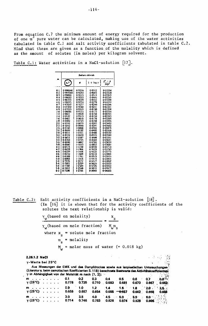
-114-

From equ~tion C.7 the m~n~mum amount of energy required for the production of one m pure water can be calculated, making use of the water activities tabulated in table C.l and salt activity c.oefficients tabulated in table C.2. Mind that these are given as a function .of the molality which is defined as the amount of solutes (in moles) per kilogram solvent.

Table C.l: Water activities in a NaCl-solution [17].

Sodium 'Alorid1

0·1 0·99664{i I 0·9324

I 0·8912 0·03354

0·2 0·993360 0·9245 0·8661 0·03320 0·3 0·99009 0·9215 0·8511 0·03303 0·4 0·!186112 09203 0·8406 0·03295 0·5 0·98355 0·9209 0·8~32 0·03290 06 0·98025 0·9230 0·8278 0·03~92 0·7 0 !176!12 0·9257 0·6240 0·032!16 0·8 0·97359 0·9288 0·8211 0·03301 0·9 0·97023 0·9320 0·6190 0·03308 1·0 0·!16686 0·9355 0·8175 0·03314 1·2 0·9601 0·9428 0·8158 0·03325 .... 0·9532 0·9513 0·8159 0·03343 1-6 0·9461 0·9616 0·8178 0·03369 1·8 0·9389 0·9723 0·8206 0·03394 2·0 0·9316 0·9833 0·8245 0·03420 2·2 0·9242 0·9948 0·8291 0·03445 2-4 0·9166 1·0068 0·8344 0·03475 2·6 0·9089 1·0192 0·8402 0·03504 2·8 0·9011 1·0321 0·8466 0·03532 3·0 0·8932 1·0453 0·8535 0·03560 3·2 0·1111~1 1·0~7 O·llf.oll 0·0~~91 H 0·8769 1·072~ 0·8684 0·03621 3·6 0·8686 Hl667 0·8766 0·03650 3·8 0·8600 1·1013 0·8852 0·03684 4·0 0·8515 1·11~ 0·8939 0·03713 4·2 0·8428 1-1306 0·9029 0·03743 4·4 0·8339 1·14~ 0·9122 0·03775 4·6 0·8250 1·1608 0·9218 0·03804 4·8 0·8160 1·1761 0·9315 0·038J3 5·0 0·8068 1·1916 0·9415 0·03864 5·2 0·7976 1·2072 0·9517 0·03892 .5-4 0·7883 1·2229 0·9620 0·03920 5·6 0·7788 1·2389 0·9726 0·03950 5·8 0·7693 1·2548 0·9833 0·03977 6·0 0·7598 1·2706 0·9940 0·04003

Table C.2: Salt activity coefficients in a NaCl-solution U8]. (In [16] it is shown that for the activity coefficients of the solutes the next relationship is valid:

y (based on molality) w

x s

------------------------------ ~ ----y (based on mole fraction) M m w w s where x = solute mole fraction

s m = molality

s M = molar mass of water (= 0.018 kg)

w

2.28.1.2 NaCI '.' y-Werte bei 2s•c , .-:ti:

Aus Messungen der EMK und des Dampfdruckea sowle aus isopieatischen Untersuchungen-~; (üteratur s. beim osmotischen Koeffizienten S. 118} betec:hnete Beatwerte cJe. Aktivitltsltoefflzient~' yin Abhängigkeit vonder Molalität m nach (1, 2]: · . . · : c • ::'·

m ... 1 (2~·c>

m ••• y (26°C}

m ••. y (25.C}

. ~ ." .. t' 0.1 0.2 0.3 0.4 0.5 · 0.8 0.7 · O.ltfl.:. 0.778 0.735 0.710 0.693 0.681 0.673 0.667 ' 0.~;'

0.9 1.0 1.2 1.4 1.8· 1.8 '2.0. ·, 2,.$..~ 0.659 0.657 0.654 0.656 -o:657 0.662 . 0.66f4 0 ••

3.0 3.5 4.0 . 4.5 5.0 . 5.5. 0.714 0.746 0.783 0.826 0.874 0.928

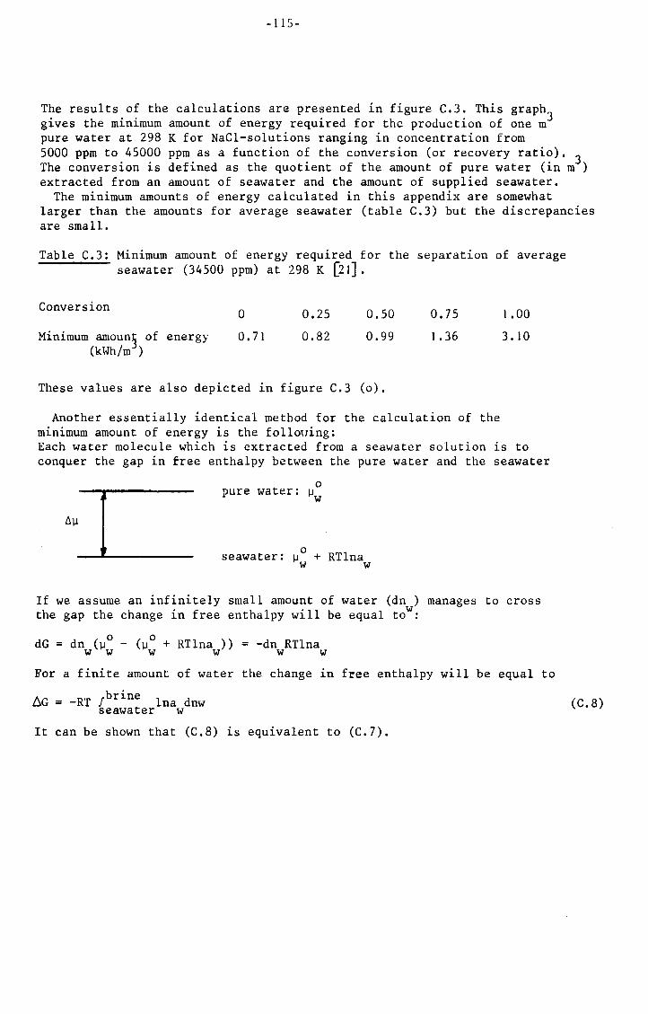
-115-

The results of the calculations are presented in figure C.3. This graph3 gives the minimum amount of energy required for thc production of one m

pure water at 298 K for NaCl-solutions ranging in concentration from 5000 ppm to 45000 ppm as a function of the conversion (or recovery ratio), 3 The conversion is defined as the quotient of the amount of pure water (in m ) extracted from an amount of seawater and the amount of supplied seawater,

The minimum amounts of energy calculated in this appendix are somewhat larger than the amounts for average seawater (table C.3) but the discrepancies are small.

Table C.3: Minimum amount of energy required for the separation of average seawater (34500 ppm) at 298 K [21].

Conversion

Minimum amoun§ of energy (k\.fu/m )

0

0.71

0.25

0.82

0.50

0.99

These values arealso depicted in figure C.3 (o).

0.75

l. 36

Another essentially identical metbod for the calculation of the minimum amount of energy is the follouing:

1.00

3. JO

Each water molecule which is extracted from a seawater salution ~s to conquer the gap in free enthalpy between the pure water and the seawater

0 pure water: 11 w

0 seawater: 11 + RTlna w w

If we assume an infinitely small amount of water (dn ) manages to cross w the gap the change in free enthalpy will be equal to :

dG= dn (11° - (11° + RTlna )) = -dn RTlna w w w w w w

For a finite amount of water the change in free enthalpy will be equal to

brine ÖG = -RT J lna dnw (C.8) seawater w

It can be shown that (C,8) is equivalent to (C.7).

------------~ ---- ---- -- ---------

MINIMU~

A."'iOUNT OF ENERGY 3 (kWh/m )

3

2

1

0 0

fig. C.3: Minimum amount of energy required for the extraction of pure water from a NaCl-solution at T=298 K.

0.2 0.4 0.6

40000 11

35000 "

30000 11

25000 11

20000 " -

I

15000 "

10000 11

5000 11

CONVERSION

0.8 1.0

-117-

APPENDIX D

Product-information on membrane modules for seawater desalination

Recieved from:

ESMIL International BV

De Boelelaan 7

P. 0. Box 7811

1008 AA Amsterdam

(PERMASEP)

PROMAC Nederland BV

Oude Stationsweg lSA

5300 AA Zaltbommel

(HOLLOSEP)

-118-~ .. .

•. ' ,., .......... ~ ...... ~·-- ....... -~---~-·-· -- !...~-- _..,_ •. ---·· -- --·- '''-~- ••.• ·••"'

m ,@~~ I

Product Bulletin No. 264

'

I iDu Pont Company, Polymer Products Dept., Permasep* Products, Wilmington, DE 19898

PERMASEP®PERMEATOR MODEL NO. 6440..016 N

4" DIAMETER 8·10 PERMEATORS PRODUCT SPECIFICATIONS

Membrane type 8-10 aramid Membrane configuration Hollow fiber

Shell dimensions 5%" 00 x 4%" 10 x 48-112" long (14.3 cm 00 x 11.75 cm 10 x 119 cm long)

Shell material Filament-wound fiberglass epoxy End plates and segmented rings Fiberglass epoxy

Connections Feed and product, 1/2~ female, NPT

Brine, 3/8" female, NPT Brine sample, 1/8" female, NPT

Permeator weight. lilled with water 50 pounds (22.7 kg)

Operating_ position Horizontal or vertical

Initia! product water capacity' 1.600 gpd (6.05 m3 I day) nomina! + 1 5%

Salt passage' :1501.5%

Rated operating pressureu 800-1.000 psig (5.515-6.895 kPa)

T emperature range3 32°-95°F (0°-35°C)

pH range3• continuous exposure 4-9

Minimum brine rate• 2,000 gpd (7.57 mJ/day) 13,200 gpd (12.11 m3 /day)

Maximum brine rate 15,000 gpd (56.78 m3 I day)

·sa.oo on oparalion wolhaleed of 30.000 mg'l NaCI. 800 P&IQ (5.515 kPa. 77' F (25'C). a na 30-., conversoon. standara lest condoJoons IRaled operat•ng pressure vaoes w•th leed water lerJl>eralure 'For operall()(l OUISlde tnos range. consuil PerT.asop• Produels 'Bnne rale tor typocal seawater I Dnne rate tor hlghty Drackosh walers and concen1rated wasJe streams

BrineOutlet EpoxyTube

f309 6/81 ~ . .....,. ___ _ . .

· • •A.g. U.S. PIL & Tm. 011

..._,lnU.s.A

"'"'·~··-·--~~-

-119-

276 No. ___ _

Ou Pont Company, Polymer Products Dept., Permasep* Products, Wilmington, DE 19898

PERMASEP® PERMEATOR

Nolee:

MODEL NO. 6840-063N 8" DIAMETER B-10 PERMEATORS

PRODUCT SPECIFICATIONS

Membrane type Membrane conti uration Shell dimensions

Shell material End plates and se Connections

Permeator weight. tilled with water Operatin position

fnittal product water capacity'

Salt passage' Rated operating pressure2· 3

Tem erature range3

pH range3• continuous exposure Minimum brine rate•

Maxtmum brine rate

B-10 aramid

Fiber lass epoxy Feed, product and brine 3/4" female. NPT Bnne sample. 3/8"female. NPT 225 pounds ( 102 kg) Horizontal or vertical

6,300 gpd (23 85 m3 /day) nomina! ± 1 O'l-o

,., 1.5% 800-1,000 psig (5.515-6.895 kPa)

4-9 6,000 gpd (22.71 m3 /day) I 10.100 gpd (38.2 m3 /day)

40,000 gpd (151.4 m3 /day)

•eased on operahon Wllh a leed of 30.000 mg/1 NaCI. 800 psog 15.515 kPa). 77"f t25"Cl. and 30'1b conversoon. standara test condohons 'Rated operatong ptessure va roes wllh leed water temperafure 'for operatoon outsode thrs range. consun Permasep Proaucts •enne rate tor typocal seawater I brone rale tor hoghly braclush waters and concentratea waste streams

'O'Ring

Feed Brine Sample Shell End Plate

1182

Hollew Support Product Poreus Support Screen End Plate

Bleek

c®P]Hl> -.. ·-·-' "Reg U.S. Pal. & Tm. 011

Ptinlltd 111 U. S.A

I --

-120-

..

SPECIFICATION OF HOLLOSEP

HR SERIES

Type High Rejection High Flux

~R5155 "---~ / \ 'HR8355 Model HR5259 ~R5355( HR5230 HR5330 HR8330

'----------- ------ ....____ ___

Module

Number of Element 1 1 1 1 1 1 1

Size. Diameter mm 144 210 210 305 150 150 295

Length mm 397 816 1216 1330 840 1240 1320

Weight. Filled with Water Kg 25 30 40 125 21 31 100 -- -

Materials

Vessel FRP FRP FRP FRP FRP FRP FRP

End Plates SUS304 SUS316 SUS316 SUS316 SUS304 SUS304 SUS304

Connection. Female •1

Feed PT~ PT~ PT~ PTY. PT~ PT~ PH~

Product PT)1 PT~ Pn~ PTY. PT~ PT~ PTY.

Concentra te PTYa PT% PTYs PHé PTYs PTYs PTY.

Product Flow Rate •2 m3 /D 1.0 2.2 3.6 10.0 9.0 15.0 40.0 .--~

-...,_ ------ 99.à\ Salt Rejection •2. • 3 % (99.0. (~?·O' (990' 90.0 90.0 90.0 ..._ __ .- -

Test Condition

Feed Water. Nacl Solut1on ppm 35000 35000 35000 35000 1500 1500 1500

Pressure kg/cm2G 55 55 55 55 30 30 30

Temperature ·c 25 25 25 25 25 25 25

Recovery ratio % 30 30 30 30 75 75 75

Oparating Conditions

Max. Pressure kg/cm2G 60 60 60 60 40 40 40

Temperature Range 'C 5-40 5-40 5-40 5-40 5-35 5-35 5-35

Concentrata Flow Rata Range •5 m3 /D 2-10 3-60 5-90 15-150 3-60 5-90 15-150

Feed Water Oualities

Max. Fouling Index 4.0 4.0 4.0 4.0 4.0 4.0 4.0

pH Range.s 3-8 3-8 3-8 3-8 3-7.5 3-7.5 3-7.5

Residual Chlorine ppm 0.2-1.0 0.2-1.0 0.2-1.0 0.2-1.0 0.2-1.0 0.2-1.0 0.2-1.0

., According to your request. the temale connections are changeable to NPT threads in same fitt1ng size.

•2. The product flow rate and the salt rejection indicate minimum values obtained under the test conditions two hours

aftar putting the module into the initial operation.

• 3 The salt rejec tion de fin es the product quality. being indicated in the following formula.

( 1

_ salt concentration in product water ) X 1 OO. salt concentration in feed water

• • The material used tor the parts which are in contact with high sahnity water is SUS31 6.

• s. The concentra te flow ra te range is lim1ted by the quahty and the temperature of feed water.

•6 pH range is hmited by the feed water quality.

-121-

HM SERIES HA SERIES

Low Pressure Type H1gh

Rejection

High

Flux H1gh Flux

HR31 10 HR51 10 Model ( HM8255 HM823Q• HA5330 ' HA8130 I

Module

1 1 Number of Element 2 2 1 i

' 1

I

90 140 Size. Diameter mm 305 295 150 ' !

295

420 420 Length mm 2640 2630 1240 I 1320

4 1 1 Weight. Filled w1th Water kg 205 175 31 100

Materials I

FRP FRP Vessel FRP FRP FRP FRP •4

SUS304 SUS304 End Plates SUS304 SUS304 SUS304 : SUS304

Connection. Female • 1

PHe Pn~ Feed PT 1 PT 1 PT~·2 PH<

PT3i PTY:i Product 2-PP4 2-Pn:o PT~·2 I PU4

Pn. PTYa Concentrale PT 1 PT 1 PPá PH<

0.3 1.0 Product Flow Rate •2 m3/D 25.0 110.0 20.0 540

90.0 90.0 _..--,.---.....,

Salt Rejection •2. •3 % / "99.0. 90.0 /'

90.0 90.0

Test Conditions

500 500 Feed Water. NaCI Salution ppm 35000 1500 1500 1500

10 10 Pressure kg/cm2G 55 30 30 : 30 i 25 25 T emperature "C 25 25 25 25

30 30 Recovery ratio % 30 75 75 ' 75 i

Oparating Cond1tions i i

15 15 Max. Pressure kg/cm 2G 65 40 40 40

5-35 5-35 T emperature Range "C 5-40 5-35 5-35 5-35

0.3-3.0 1.0-10.0 Concentrale Flow Rate Range •5 m3 /D 35-120 40-120 10-90 i 25-150

Feed Water Oualities

4.0 4.0 Max. Fouling Index 4.0 4.0 4.0 4.0

3-7.5 3-7.5 pH Range •6 3-8 3-8 3-8 3-8

0.2-1.0 0.2-1.0 Residual Chlonne ppm 0.2-1.0 0.2-1.0 0.2-1.0 I 0.2-1 .0

• Model HM8230 available on Nov. '83.

GENERAL PRECAUTIONS

• Keep the HOLLOSEP away from direct sunshine.

• Since the HOLLOSEP is tilled with preservative solution to keep its performance. be sure to

discharge perfectly the solution prior to use.

• Do not freeze or dry the HOLLOSEP at all times. •

-122-

APPENDIX E

The use of Weibull-functions in windturbine output predictions

It appears that the windspeed frequency distribution (f(v)) of many windregimes can be approxirnated by Weibull functions [56]:

where: k = Weibull shape factor c = Weibull scale factor

The cumulative distribution function (F(v)), which indicates the probability that the windspeed v is smaller than or equal to a given wind­speed v', is equal to:

V V k F(v) = J f(v')dv' = 1 - exp(-(-) ) 0 c

The average windspeed (V) can be calculated by means of the next integral:

-V =

or

00

J v f(v)dv 0

v = cr(l+llk)

r is the so-called gamma function, a standard integral.

Employing equation E.4 equation E.l can be written as:

k k-1 k k f(x) = kr (1+1/k)x exp{-r (1+1/k)x }

where: x = v/v = the dirnensionless windspeed.

Thus the windregime can bedescribed hy two parameters: the average windspeed v and the shapefactor k.

(E .1)

(E. 2)

(E. 3)

(E.4)

(E.5)

k~ 2 e.g. the Netherlands (this result is the so-called Rayleigh-distribution)

k~ 3.5 trade winds e.g. the Cape Verdian Islands, the Netherlands' Antilles.

The average energy output of a windturbine (E) can be calculated from the following integral:

00

E = T J P(v)f(v)dv 0

where: P(v) represents the power output curve of the windturbine as a function of the windspeed and T is the period concerned. A handy dirnensionless entity to express the average windturbine output is e t which is determined by the windturbine design and the windregime. sys

E = (c n) l/2pAV

3T p rnax

(E. 6)

(E.7)

-123-

In [55] severa1 expressions for e have been derived for severa1 shapes syst of the power output curve:

1) Idea1 output curve The analytica! expression for the power output curve is given in (4.27). The expression for e is: syst

e syst

with

G k 3 Gx k k e- x dx + x ( e- r - e -Gx f )

r

G • rk(J+ r l e t Is depicted in figure F.l in appendix F as a function of the sys

(E.8)

dimensionless rated windspeed x for several values of the shape factor k (x =O·x =oo) r c , f

2) Constant torque laad (e.g. pos1t1ve displacement pump) The analytica! expression for the power output curve is given in (4.16). The expression for e t is: sys

e syst

with G = rk(l+l/k)

e Is depicted in figure F.2 in appendix F as a function of the syst

dimensionless design windspeed xd for several values of the dimension-

less rated windspeed xr and shape factor k (xf=oo), Furthermore, the

cut-in speed is related to the rated windspeed by the fact that P =P . • 3 i.e. the constraint imposed by the RO-membranes. max m1n

. (E. 9)

3) Constant power output (nat mentioned in [55]) The analytica! expression for the power output curve is given in (4.10). Substituting this expression in (E.6) we get:

E = T(c n) l/2pAv3x3 xfxf f(x)dx (E.lO) p max r r

With the definition for e (E.6) and E.2 we can derive an expression for e : syst syst

-124-

3 k k e =x {exp(-Gx) - exp(-Gxf)} syst r r (E.ll)

e Is depicted in figure F.3 in appendix F as a function of the syst

dimensionless rated windspeed xr for several values of the shape factor k (xf=oo),

-125-

APPENDIX F

Graphs of e t for the considered configurations s s

I

i·· I

I '

T

0,2 . . [

·- -- r -- .,-·- -·

i

r

\

1

I I I

l. I I

.. ,.- -I I !

l ~-· .. ----1

I

i I I I ... I I I

- t-·

. ..-:

' 1 ~. '

't

f :

: I -127- . • i i I I

. l 11 i r' . 1

1

• • ; i'

11

• 1

1 !: ; . I I ·' I I • . • r I I 1 ! ! r •

FIG. F2a: -~-e~l~ :· -f~~-~ ~-~~ip. dHbir~ wi[th i~ ~~~~.·.· S.fan.t t~rq~~ i~-~d. A~~.·tr-~.·--.•. :~~--re~tric,tio . .n llt\),:1. tIp • , .. :3 ~ . .I; vafi~ble: d~!>ign jwindl sp .. eer .... ·: L ..

I : I \ ma:K : rm~n I ! . : I . I I : • . I

: -·' 1

parameter: J.1ated'wind 1 spee..l:•kl= '),I;, 1

1 ! I · I : 'j.

1 ' •

1 . , ~"'' r I 1 .

.... r . l .. I : . -r .. : I· T ·:i~· .. ! : . I I , .. ,. I ,

I I I I • .

I I : I : . i"C T ....

1

- -.. : : 1 : ~·r ... ' I I I ..

I I I ' I -· . . 'l ! 'j ! ''I' C·- . .. - ... '

- I

. . ... , .. I 1. 1

. i

1

: l ' .: I I j \ ..... T r r ' ·[·· :··r . I .. : .......... t·'·j• I I I I ' I .. ; . I I I ' i

I I ; I ! I i • "I . 'I . ' . I . I i . i . - -· .• >~+···· ' p I I I I I ' I .. I I ' i ~ I : . ,

···; .. 'j· .l L/ -~ ~ r·

I ~I . . I

, .. ï ~:

:} 111

i ...

--·-ï .. , . r·· · ! i . t

"I. . Ï

I . . I I

L.,r,t r-~---~~ .. ·i··:··r·

; ·1 ' i

1 r !

r··--. I

I

·. f ~--- ·-r ---· -I ....

· · · I 1

l I

T'1.p;;Á1a J

' I ' I :--. I 11

I I .. I· -- -r I I

I . I ...... ; · . i I I i •

r i ' . t 1 .• ---r-1 .. ... -r· I r·-. i

!

., ' ' i.

I I I

1

I i ,. I

i !

I I I --·~

;.J iJ. I

I I. I

i I -·----r I

·!

..

"1·

·- -· ~ ·- ~ ··-

l I I I I I I ! I

/

' , • I -128-

1

1 ' I ' ' ' ' I I ! i 1 ; I _ : FIG. F2b; -j-esysf f9r

1 a w.~nd \,llbine! w+ç~ a c1n~taft: ·torql,le ~~ofld un<hl tll; .. ·: ..

: [ 1restfiction that P. =3P. 1; va,iablf: de~ignlwind spee~; 1 i· : • ' 1

1 I Illax l m1.n; 1 • ' 1 I I , ' I- -: -~- I jpar et;erj; ra 'èd' win9 sre~d;j ik= 12. I -. t- - --- ;·--· ·--ï--. ·-+-~ :--

: .. I . - I I 1 I I I I I ' [ I I l ! ! ! I I ; '

I I ' I I I ' I ' I I \ I ! '

' : i l ' I I . I I I I 1 ' --7- ·---_--- ·- r --:---~-- ·_ j---1 •. _ -- -- 1 ;·- ~--- •· 1 r·--. -f - --~---t -··---··--- --

-. --- ... · i · ·- · - : · I I . I ' . . I ; . ' : l : . : ! ! ' I . ' I

. r_·- :--.~- -+-:----_•1- ----- :-- --~---:·· ··-· 1- - _j j-

1

.. ~ . . . . . ' . I i : I " ... , ....... -~----- . -- --- .j_ - . - - - - r· --·--- -- - , .. ~~. .. ---· . ! • . I . :

1

1

· ~--·········· · ··r I ~ ·· 1 ·r

, ........... -- .. _ ...... -----·-- ---~-- ..... I . . ·1· ·- ........ , ..

I ' ' '

I • 1 I , I

- · 1 · · 1. 1

--------l·--: ... ~1---·- .; -- -.. -- . . . -1-- : .. : 1. f ' I . ' • I i I

.. : - : t· ! . I ' I I ··:t --~ I

! i

: I ·--r · ·- 0

:-· --~----- ----]- -. --~ I t ·- :11 I

i- I ·· ·>i! .,-_1· .... ,.. l_j __ l: ___ '.... . ..... ' ' ' . ' . . . ' . ' . - -~. . . . .

:. : I ~-:- • ---:--- --·r-- ---- ----~

'

- ----- --- . . - . I . < ' I

I .. l'- .. T I . ; I ,.

-- -• . -; I - ······ i t · · • ·-

'

i I I I _T_] __ ----:---T ___ -r- ... -. --~----_! ----- . - !

· ----- -- -- -- · 1 - • . - i · I ·- .... -- . I . ' . . ·r·. ; . '

· ··1 : 1 · 1 · ·

--·c---ri_--------,----~ -+ -- . i - . : -- ( --' I ' I . • . . l ; : :

' ' ' I 1

-.;,. I ~ '

I i

I - -~~----- ---- ..... , .. I !

' I

c:.;>_ ~

j· -- I I I

!

I .l

~... +---- - - --· ------·-

i

---~- --

! j·

I

I . I

i

I-

I ~

Ln C?~

I l

i I'"

' i ' j"' : r

'

!. ··-'. _, ___ 11

j !

i ~ l - . ; . . I .

l f·

·r-· !

I .j

i : I l 1

. I . ! : ... I.. _, .... j

. :

' I ··j·

I

I ' : -129- I . . : I I ; I

i ' I i ! I ! I i ' ' FIG. F2c_; I e ·1 H.fo~--- ~. win4tu_1 rbi~f~ .. ~it~~~ Jon~t-:ant_ t~rquJ lo~X- und~~ ;~he ·;··-j·~~·~---

1 sy~t i I .. I I ,. ! . . r : I . T . I .I ..•. T .• I I

i re$t.r~ct~on q.hél:t: ~ . r 3P 1 .. ; ~an..·ab.le: pe~i,'n-wi~q :sp.r~q.; i r ' I I I lmax ffi,lU : I ' l I

··---i '.. I parametef' : r~ted ~ind speed!; ~ , 3,5t . I . ' I . I : • I I ' ' I . ' I . . .

,~ I r r ' I ' I ' ···: I . I .• I .•• T i I · .. I • ,. i . . . ' I ; . I

f ....... .. --r T t·· r----,--: + . I I r· . r .. ' . j .. j .. ' I .. ' !······· ~·-·-1, ' I \ I I ! I i I ' 1 : ·1· · -1· ! ·1 1 ·r· r ·•

I

I ; I ! ' I I I

·····:··,, :····~- ·. ·• ·· --~---·- ··,!-- · ·r 1· · r 1 i . · 1 I

' . I I I I I I ~- .:1···:~~-----~- -. .. . :- . ·-r . -· I' .,.. 1 T ' i .. ---+---~f---1

' I I : ! - .î ..• ,----:··--·

1--- . -· I l -- ·r . - 1 . --r··

I . . I . . .. ·t . I I i ·

1

.. --·:· ···r· · · · --r~ -- · i :- 1 ·. . · I I • , •

1• I I

. I I : I ---~---+- ... -r--·-- i -... - ! .. . .. .. . T-

.... : ... T ·: . ·1· · ' . I i ... . : : t . I ·--:--~-,l·---;-+-- -r· · l i I ' · ·· ·· :!1

I . I I i -··T· ·:-···· :···l . • . . ' . '. ; ....:t

i . i I • . : I -_T __ T_T ______ · T .. I u

: I : . . I f ,_.

---~-.~·1· - -··--:r--- ·+· . - ~-' . I

~---L~·r··•-T: --_- -··--i'

I i .I ' I I I

-lLJ_ -i

• ~ •-• I .... [ .

~~\'' I ' ! I !

! : . ; ' t : ! : ' . 1 : ~ .. \ • · I ·· ' I 1 • • · • "" ... • .,... ·•·--~

I ! ' 'i • : "! :, I !

: .. \

I I U!l

I-~ ..

.rfi I. ! I I I '

· I ... .. t

--·:·T ··I I ~ .. r--··· . i I -,--~ -- . i

I i·- _J

I -1 ' I

I I . I I ·---~- ..... .. .. ,

I' .. "l ~- 1 '·

I .

I

t·

I

I

'ï I

' i !

. . ... ·I­! !

.. -r·.

I

I

i

i

I !

I

.l '. I.

i

1 • ,l. 1 · ~ ··· I • I • •

I ' 1·-·-

-·. ,._

- ~ ~~ . .

.. ·i + .. I I . r·· .i. ....

! I , , .... ,~ .· I . "1

r···· •• ~ L -- •

r·· I I . ' ; : . -130- I i . ; : I i'

~ 'I \ ! 1

1

1

! i i ! .. 1

• I ! : •. t • • ! I i ! I I FIG. F3. ~esyst -~r :W~F~,b~~ w~t.h a:crst<l:~t pore~ or-tpu~ a~- .. -·T·-:-r--r·

fuictil qf Fh~ ~·tFd windl•pee.d fo, sevfral r·+~4· ff ,~. I i .... !

i I / 13ha_ pe fflçtorJ.· · I l • I_ ' / ·_ . 1 I ! ( · .' : · - 1 · r- · i 1 __ 1_ ! . ~ . 1 1 t. I.. 1 .

- , .... ~r-··: ~ ·---~--·-- . [ ·i'-j 1 \ I I \ ! \ l 1

1 •

I I I I I I • I I I I I I '

. I . ,~ I . I· .. . . ~- ~ ........ .. [" I ~ l ' I >f-i ... 11 i IJ··,:IH·~

; -1 .. ,. i . i '- '[· I I I I .· . ..,. . • . . . . .... l . i . . . .... . . i '

--.··;--·1· ·:· ·-r- ' I ·I' I ; : I I ! r-- .. ~-r -, -r-- --T · i : ·u; - , ·

Ir, : - .1. ... -~----l-- ___ .J -- r-- -- .i .. i~ • ' I 1

I 1 \ l ·

t ' I I . . l

• • I I ........ ,.. ·--r ·1 1 .

I ' I 0 . I I N

-~·l:'j .... :_---·i·--·----... 11_ . "1. ·- i . . ..

• I : f ! I I : . '

..... r I

~- --\··

_, .. I I I

·-·r·· ~-

1 '

-1-. ·-: I I : ,

I I I ;---·~- •• ·· · : · 1 · - r 1

... : ---·r- -:-, .. - . :·· + . I

,. • ·r· i 1· ·-r··· •1· · .... :-r +- :

' I ""'I 1\ i . I . riS Sa ! · I 1 ·-·r ·, · · 1 l .

I --- ~ Î I I I I

I ··t-

i i

j· I

I ·j·' :. !

.... T -·~- --:·t-;---

1 I , I'

I

-- .. - 1- .

I . . !

I I I ,

j. I .

~-\ . . --. I

· f · I I I

l I . I .

- :·- .L .. f---t ... I : I , ' I !· ., ..

-131-

APPENDIX G

List of raferences

1. 'Waarom mernbraamfiltratie?', C.A. Smo1ders, pt-procestechniek, ,ll, 1978, 3_62-368

2. 'Saline water distillation processes', A. Porteous, Longman Group Limited, London, 1975

3. 'The economics of wind-powered desalination systems', T.A. Lawand, Report no. T-36, june 1967, revised sept. 1967, Brace Research Institute of McGill Univarsity

4. 'Putting the wind to work', Chi11cott, Engineering, 206, 1968, 760-761

5. 'Le dessalament de l'eau de merpar !'energie éolienne', s. Salomon, L'eau, 22, 1968, 5

6. 'The application of wind energy systems to desalination', E.A. Cadwallader, et. al., 1977, Wi1liamson Engineering Associates Inc., Navarre, Fla, prepared for Office of Water Research and Technology, Washington, DC

7. 'A wind powered water desalination plant for a small island community at the German coast of the North Sea: design and working experience', G. Petersen, et. al., Conference: 'Energy for rural and island communities', Inverness, 1983

8. 'Nutzung der Windenergie zur Meerwasserentsalzung~ Projekt­beschreibung einer Prototypan1age', s. Fries, G. Petersen, G.K. KS, 1978

9. 'Wind and solar powered reverse osmosis desalination units. Description of two demonstratien projects', G. Petersen, s. Fries, J. Molin, A. M~ller, Desalination, 21, 1979, 501-509

10. 'Sea water desa1ination powered by wind energy', s. Fries e.a., Praeeedinga of the International Colloquim on Windenergy, Brighton, U.K., 1981

11. Report third international meeting on teststations for SWECS, S.J. de Boer, Pel1worm, 3/4 may 1983 (WB83/WM-5294), TH'r

12. 'Dessalement et energie nouvelles', A. Maurel, Desalination, 21, 1979, 489-499

13. 'The exergy methad of energy systems analysis', A.E. Ahern, Wiley, New York, 1980

14. 'Principles of desalination', 2nd edition, K.S. Spiegler, A.D.K. Laird (ed.), Academie Press, 1980

-132-

15. 'Fundamentals of water desalination', E.D. Howe, Marcel Dekker Inc., New York, 1974

16. 1 The principlesof chemical equilibrium', K. Denbigh, Cambridge Univarsity Press, 1971, 3d edition

17. 'Electrolyte solution', R.A. Robinson, R.H. Stokes, London Butterworth's scientific publications, 1959, 2nd edition

18. Gmelins Handbuoh der Anorganischen Chemie, B. Auflage, Natrium, Ergänzungsband Lieferung 7, Halogenide, 1973

19. Collegedictaat Thermodynamica, H. Gijsman, TH Eindhoven, 1978

20. 'Calculation of some thermadynamie properties of sea salt solutions at elevated temperatures from data on NaCl solutions', R.W. Stoughton, M.H. Lietzke, Joumal of chemical and engineering data, vol. 10, no. 3, 1965

21. 'Thermodynamic properties of sea aalt solutions' R.W. Stoughton, M.H. Lietzke, Journal of chemical and engineering data, vol. 12, no. 1, 1967

22. 'Thermodynamic properties of sea salt solutions~, L.A. Bromley e.a., AICHE-journal, 20, 1974, 326-335

23. 'Salt-water purification', K.S. Spiegler, Plenum Press, New York and London, 1977, 2nd edition

24. 'Wind, pumps and desalination', F.H. Theyse, Praeeedinga of the third Miami international conference on alternative energy sources, 15-17 december 1980

25. 1Dessalement par osmose inverse associée à l'ene~gie atomique', A. Maurel et. al., Journée d'étude sur l'energie solaire et le dessalement, L'association Francaise pour l'etude et le développement des applications de l'energie solaire, Paria, 1984

26. Energy recovery system with hydraulic turbine for reverse osmosis plante, Ecowatt, 1983

27. 'Desalination and renewable energies-a few recent developments', J.J. Libert, A. Maurel, Desalination, 1i, 1981, 363-372

28. 'Desalination and energy', J.J. Libert, Desalination, 40, 1982, 401-406

29. 'The role of energy and economics in water conversion', F. Kranebitter, Desalination, 2Q, 1979, 501-514

30. 'Comparative energy requirements and economics of desalting processas basedon current and advanced technology', P. Gluekstern, Desalination, 40, 1982, 63-74

-133-

31. 'Economie aapacts of membrame processes', O.K. Buros, Desalination, 2Q, 1979, 595-603

32. 'Desalting seawater and braokiach water: a coat update', T.J. Larson, G. Leitner, Desalination, 2Q, 1979, 525-539

33. 'A oomparieon of the relativa economics of sea water desalination by vapor oompreesion andreverse osmosis for small to medium plante', R. Mati, U. Fisher, Desalination îi, 1981, 137-151

34. 'Process selection guide to seawater desalting', D.R. Finnegan, W.M. Wagner, Desalination, ~' 1981, 29-48

35. 'Selection of desalination technology, a decision analysis approach and a casestudy', A.A. Bushnack, et.al., Desalination, 2Q, 1979, 483-498

36. 'The effect of a variable power input on the performance of a reverse osmosis desalination unit', R. Alward, E.R. Lising, T.A. Lawand, 4th International Symposium on Fresh Water from the Sea, vol. 4, 1973, 25-34

37. 'Unsteady state oparation of areverse osmosis desalination unit', E.R. Lising, R. Alward, Desalination 11, 1972, 261-268

)8. 'The minimum energy requirements for sea water conversion processes', G.W. Murphy, Office of Saline Water, Research and development progress report no. 9, april 1956

39. 'Thermodynamica of some desalting processes', B.F. Dodge, A.M. Eshaya, Advances in chemietry series, ll• 1960

40. 'Reverse osmosis membrame research', H.K. Lonsdale, H.E. Podall, Plenum Prees, New York and London, 1972

41. 'Status of raveree osmosis technology', J.c. Schippers, The Netherlands Waterworks Testing and Research Institute: KIWA N.V.

42. 'Kwaliteitsverbetering door hyperfiltratie', J.c. Schippers, A. Kostense, H2g, 14e jaargang, nr. 25, 1~81

43, 'Reverse osmosis 1 , J.C. Schippers, The Netherlands Waterworks Testing and Research Institute; KIWA N.V., Research prograas report, september 1980

44. 'Review of raveree osmosis membrames and transport models', M. Soltaniek, W,M. Gill, Chem. Eng. Comm., vol. 12, 1981, 279-363

45. 1Reverse Osmosis', S. Sourirajan, Academie Prees, New York, 1970

46. 'Calculation of the expected performance of raveree osmosis plante', c.w. Saltonstall, R.W. Lawrence, Desalination, 42, 1982, 247-253

-1:54-

47. 1Conceptual Design aspects of raveree osmosis, D. Kuiper, M. Mendia, Desalination, 22, 1980, 273-289

48. PERMASEP engineering manual, Bulletin 202, 1reverse osmosis', 1982

49. 'Ein neuer Plattenmodul fÜr umgekehrte Osmose und Ultrafiltration', S. Fries, et. al., GKSS78/E/48

50. 'Membrame separation processes, P. Meares, Elsevier Scientific Publishing Co., A'dam,Oxford,New York, 1976

51. 'De membraam filtratie-index als kenmerk voor de filtreerbaarbeid van water', J.C. Schippers, J. Verdouw, KIWA

52. PERMASEP engineering manual, Bulletin 402, 'B-lO PERlVlASEP permeator, factors influencing performance', 1982

53. Toyobo, Data Sheets

54. 'Reverse osmosis in the desalination of.brackisch and sea water', H. Ludwig, Desalination, ~. 1981, 153-178

55. 'Output predietien for windturbines in Weibull distribution regimes', E.H. Lysen, Eindhoven Univarsity of Technology, Windenergygroup, R475D, april 1981

56. 'The estimation of the parameters of the Weibull wind speed distribution for windenergy utilisation purposes', M. Stevens, P.T. Smulders, Wind-engineering, 1, 1979, 132-145

57. 'lntroduction to wind-energy', E.H. Lysen, Steering Commitee Windenergy Davaloping Countries, SWD82-1, Amersfoort, august 1982

58. 'Review of conversion systems used in autonomous wind energy systems•, J.A.N. de Bonte, EUT, R5930/EM82-35, february 1983

59. 'Autonomous wind diesel systems in rural areas in the Republic of Cape Verde', J.A.N de Bonte, M. Dieleman, CWD, march 1984

60. 'Measurements on a diesel generator set for an autonomous wind diesel system', J.A.N. de Bonte et. al., Eindhoven Univarsity of Technology, R-623-D/EMV83-31, november 1983

61. Private communication, Ir. Drs. J.P.P. Tholen, Esmil International B.V.

62. 'Tie kostp~s van windenergie', J. Daneels, Benelux Economische Unie, Nationale Windenergie Conferentie Noord~kerhout 14/16 september 1983

63. "Zeewaterontzilting met behulp van zonne- en windenergie" TEBODIN februari 1981 Studie verricht in opdracht van het ECN.