Eindhoven University of Technology

MASTER

Design of an automated guided vehicle supporting an order picking robot for the warehouseof the future

van Loon, T.J.

Award date:2019

Link to publication

DisclaimerThis document contains a student thesis (bachelor's or master's), as authored by a student at Eindhoven University of Technology. Studenttheses are made available in the TU/e repository upon obtaining the required degree. The grade received is not published on the documentas presented in the repository. The required complexity or quality of research of student theses may vary by program, and the requiredminimum study period may vary in duration.

General rightsCopyright and moral rights for the publications made accessible in the public portal are retained by the authors and/or other copyright ownersand it is a condition of accessing publications that users recognise and abide by the legal requirements associated with these rights.

• Users may download and print one copy of any publication from the public portal for the purpose of private study or research. • You may not further distribute the material or use it for any profit-making activity or commercial gain

Design of an automated guidedvehicle supporting an order picking

robot for the warehouse of the future

DC 2019.068

T.J. van Loon BSc., 0861750

Committee:prof. dr. H. Nijmeijer (chairman)

dr. ir. P.C.J.N. Rosielle (thesis supervisor)dr. ir. R.H.J. Peerlings

ir. M.M.G. van Lith (advisor)

Eindhoven University of TechnologyDepartment of Mechanical Engineering

Dynamics and Control group

21 June 2019

Summary

Web shops offer customers the luxury of shopping from the comfort of their homes. Theorders sent by customers have to be fulfilled by order pickers. Order pickers compile ordersfrom individual items which are stockpiled in a warehouse. Companies want to automatethe order picking process in order to make their entire supply chain more efficient.

Warehouse automation is often based on conveyer belts that transport items to pickingstations, where order pickers compile the individual orders. Such systems reduce the timethat would otherwise be spent by an order picker walking through the warehouse with atrolley. However, such order picking systems are a large investment, and are not scalable.

Smart Robotics, EPhi and Nobleo Technology want to create an order picking robot.This robot should be able to perform all tasks a human order picker performs as well:Navigating autonomously through a warehouse, picking items from racks, and leaving thecompiled order at a drop-off point. A prototype has been built, which consists of an AGVsupporting a 6 degree-of-freedom robotic arm, and a conveyer which holds a container.

To improve the order picking robot, front- and rear wheels suspensions are designed.With the new suspension design the order picking robot can corner faster, and is morerobust to floor surface irregularities. The prototype AGV has two individually driven rearwheels, and two casters at the front. The newly designed AGV has its rear wheels driven,and its front wheels steered using an Ackerman linkage. This decouples longitudinal andlateral motion, which is beneficial for maintaining velocity while cornering. By replacingthe casters with steered wheels more lateral force can be exerted on the floor by the AGV.This means that the AGV can corner faster.

The front suspension is based on the McPherson strut suspension design. The wheels areconnected to uprights. On the top, the upright is attached to a damper. The centerlineof the damper points to a ball joint between the upright and a leaf spring. The leaf springis mounted to the bottom of the frame. The piston of the damper can freely rotate in itshousing. Therefore the wheel can be steered around the centerline of the damper. Thesteering is actuated by using a Pitman arm. The pitman arm consists of partial gearswhich are driven using a pinion attached to an electric motor inside of the frame.

The rear wheel suspension is built around an axle containing a steel spur gear differential.The spur gear differential is directly connected to the wheels by tubular shafts that arealso contained within the hollow axle. The axle is connected to an A-frame from the top,and to two longitudinally placed struts close to the wheels on the bottom. The weight ofthe frame is carried by two shock absorbers.

Contents

1 Introduction 11.1 Background . . . . . . . . . . . . . . . . . . . . . . . . . . . . . . . . . . 11.2 Automating the order picking process . . . . . . . . . . . . . . . . . . . . 21.3 Objective . . . . . . . . . . . . . . . . . . . . . . . . . . . . . . . . . . . 21.4 Current solution . . . . . . . . . . . . . . . . . . . . . . . . . . . . . . . . 31.5 Project aim . . . . . . . . . . . . . . . . . . . . . . . . . . . . . . . . . . 4

2 Specifications 52.1 Low cost design . . . . . . . . . . . . . . . . . . . . . . . . . . . . . . . . 52.2 Compact design . . . . . . . . . . . . . . . . . . . . . . . . . . . . . . . . 52.3 Able to support the weight of the order picking robot . . . . . . . . . . . 52.4 Robustness to rough floor surfaces . . . . . . . . . . . . . . . . . . . . . . 62.5 Safe to use around human personnel . . . . . . . . . . . . . . . . . . . . 62.6 Capable of withstanding the tire forces during travel . . . . . . . . . . . 7

2.6.1 Wheel modelling . . . . . . . . . . . . . . . . . . . . . . . . . . . 72.6.2 Load on wheels during acceleration . . . . . . . . . . . . . . . . . 82.6.3 Load on wheels during deceleration . . . . . . . . . . . . . . . . . 82.6.4 Maximum velocity during straight line driving . . . . . . . . . . . 92.6.5 Load on wheels during cornering . . . . . . . . . . . . . . . . . . 9

2.7 Able to remain operational for a specified lifetime . . . . . . . . . . . . . 122.8 Summary . . . . . . . . . . . . . . . . . . . . . . . . . . . . . . . . . . . 14

3 Overall design 153.1 Wheel force comparison . . . . . . . . . . . . . . . . . . . . . . . . . . . 153.2 Ackermann steering . . . . . . . . . . . . . . . . . . . . . . . . . . . . . . 163.3 Tire choice . . . . . . . . . . . . . . . . . . . . . . . . . . . . . . . . . . . 193.4 Wheel construction . . . . . . . . . . . . . . . . . . . . . . . . . . . . . . 20

4 Front wheel suspension 214.1 Construction of the upright . . . . . . . . . . . . . . . . . . . . . . . . . 224.2 Pitman arm . . . . . . . . . . . . . . . . . . . . . . . . . . . . . . . . . . 234.3 Leaf spring . . . . . . . . . . . . . . . . . . . . . . . . . . . . . . . . . . 24

5 Rear wheel suspension 265.1 Rear wheel drive and suspension concepts . . . . . . . . . . . . . . . . . 26

5.1.1 Electronic differential . . . . . . . . . . . . . . . . . . . . . . . . . 265.1.2 Mechanical differential using Nylon gears . . . . . . . . . . . . . . 285.1.3 Mechanical differential using Steel gears . . . . . . . . . . . . . . 325.1.4 Concept choice . . . . . . . . . . . . . . . . . . . . . . . . . . . . 34

5.2 Differential construction . . . . . . . . . . . . . . . . . . . . . . . . . . . 345.3 Axle assembly . . . . . . . . . . . . . . . . . . . . . . . . . . . . . . . . . 355.4 Construction of the A-frame and the struts . . . . . . . . . . . . . . . . . 37

6 Conclusion 38

7 Recommendations 38

1 Introduction

The current rise of web shops puts an increasing strain on logistics, with many web shopseven promising to deliver goods to the customer in less than 24 hours. These demands canonly be met because of growth in the transportation sector and various smart warehousingsolutions. In the case of web shops, the focus is on making order picking more efficient.Order picking describes the act of gathering items from a warehouse, and bringing themto a drop-off point. This is done by dedicated personnel called order pickers.

1.1 Background

In order to conceptualize the layout of a typical warehouse DSV was visited. DSV isa logistic company. A photo of the inside of the warehouse is shown in Figure 1.1.Their warehouse features many narrow corridors. These are formed by racks filled withcardboard boxes, which are accessible from the sides. The items contained in these boxesare packed in small plastic bags, with a maximum weight of 2 kilograms. Packing itemsin plastic bags is common practice in warehouses. The order pickers use slim trolleys onwhich they carry multiple container. In each of these containers they need to collect acertain order.

Figure 1.1: A typical warehouse

The corridors are 1500 [mm] wide. The trolleys are 600 [mm] wide. This means that anorder picker has the possibility to overtake another order picker who has stopped to fillsome of their containers, while still keeping 100 [mm] of clearance on each side of theirtrolley. An order picker has to systematically walk through a warehouse to collect eachorder. They gather the contents of an order in a container. To reduce human errorsduring picking, order pickers are aided by warehouse management software, which tellsthem what item to pick next. Warehouse management software helps web shops to keeptrack of their inventory, while it allows order pickers to keep track of the items theyhave to collect. Multiple orders can be combined in a batch. By fulfilling batches oforders instead of separate orders the order picker spends less time walking through thewarehouse. This reduces picking times.

1

1.2 Automating the order picking process

An order picker can easily grab items out of a cardboard box. However, a robot oftenstruggles with such a task because the location of the item in the cardboard box is notdetermined exactly. Next to this, various different items need to be handled. This makesorder picking inherently difficult for robots. This is the reason why robotic order pickersstill are are less efficient than a human order picker. However, the power of automatingthe order picking is that the process can be made more predictable, in terms of how longit takes to fulfill an order. This allows companies to optimize their entire supply chain.

Currently available warehouse automation aims to bring the cardboard boxes to pickingstations using conveyer belts. At these picking stations, order pickers compile ordersfrom the incoming cardboard boxes. Such order picking systems are a large investment,typically in the range of 10 million euros. It also takes a long time to install the systemin a warehouse, as the warehouse needs to stay in operation to avoid loss in revenue forthe company. When the system is installed, it is not scalable. This means that when thecapacity of the warehouse should increase, or when the range of products stored in thewarehouse is altered, the order picking automation needs to be rebuilt. Next to this, thethroughput of a warehouse can periodically change throughout the year, while the orderpicking automation is designed for peaks in the throughput.

1.3 Objective

Some companies envision a warehouse robot that can execute most tasks a human orderpicker can perform, including:

� Autonomously navigating through a warehouse

� Picking items from a cardboard box in a rack

� Delivering an order at a drop-off point

Buying one robot allows a company to partially automate their warehouse. The robotneeds to be designed to allow for easy commissioning by any warehouse. Robots could beused during peak moments in a warehouse, while they can be stored or used somewhereelse when the demand on the supply chain is not as large. The return upon investmentof such a robot would then be faster than buying an entire automated warehouse. Thesolution is scalable, as multiple parts of the warehouse can be automated by buying morerobots. Having robots work alongside order pickers could result in conflicts, if the orderpickers feel threatened by the robots. It should therefore be considered to divide thewarehouse in robot-only and human-only parts.

The robot should be applicable in different warehouses. While new warehouses often havesmooth concrete floors, the floors in older warehouses might have a lot of irregularities.An AGV carrying such a warehouse robot therefore needs to be robust to irregularitiesin floors. The order picking robot should be designed to operate in a warehouse withoutadditional infrastructure. The layout of the warehouse could thus be maintained, reducingthe overall cost of automating (parts of) a warehouse.

2

1.4 Current solution

Three companies, SmartRobotics, Nobleo Technology and EPhi, want to create an orderpicking robot in a joint effort. The current prototype of the order picking robot consistsof an automated guided vehicle (AGV) supporting a 6 degrees-of-freedom robotic armand an on-board conveyer which can hold a container. This can be seen in Figure 1.2.

Figure 1.2: Prototype of the order picking robot

This prototype is built out of spare parts, and is used to demonstrate the functionalityof the order picking robot to potential customers. To realize the autonomous navigationa laser range finder system is used in combination with an optical flow sensor. The laserrange finder can scan the direct surroundings of the order picking robot, ensuring thatit does not collide with its environment. The optical flow sensor features two cameraspointed at the floor, which keep track of the AGV’s orientation. This particular sensor,an Accerion Jupiter-40, can also keep track of the exact location of the order pickingrobot. It captures images of the floor surface, and therefore remembers which patches ofthe floor it has already seen. The overall dimensions of the AGV can be found in Figure1.3.

The AGV used in the current prototype of the order picking robot is produced by NobleoTechnology. The AGV’s front wheels are casters. By individually driving the rear wheelsusing electric motors, the AGV can be driven and steered. Because casters are used atthe front of the AGV, the wheelbase can vary anywhere between 460 [mm] and 520 [mm].The front track width can vary between 360 [mm] and 600 [mm]. It is therefore hard toestimate how the load of the order picking robot is distributed over the wheels of theAGV at any given point in time. This results in an unpredictable performance of theAGV during straight-line driving as well as during cornering. Figure 1.4 shows that thesuspension of the AGV is not able to support the full weight of the order picking robotwithout reaching the end stops. This leaves no room for any wheel travel during bumps.

3

Next to this, it also reduces the clearance between the bottom of the AGV and the floor.

Figure 1.3: Overall dimensions of the current AGV

Figure 1.4: Sagging of the AGV’s suspension

1.5 Project aim

The aim of the project is to design a new AGV for the prototype of the order pickingrobot. The new AGV should be able to carry the load of the order picking robot, cornerfaster than the current AGV, and be more robust to floor surface irregularities.

4

2 Specifications

The development of the order picking robot is a ’technology push’ type of project. Thismeans that the specifications for the order picking robot are not determined by a cus-tomer. The specifications for the AGV are therefore discussed in the following Sections.

2.1 Low cost design

The goal of the project is to create low-cost automation for warehouses. When the orderpicking robot turns out to be a feasible solution for warehouse automation, its designshould allow mass production. Therefore the prototype for the new AGV should be builtout of low-cost components that are readily available. The assembly of the AGV shouldbe straightforward. This also allows for easy maintenance of the AGV, which reduces thecosts for operating the order picking robot.

2.2 Compact design

The AGV should have a small footprint. This is necessary to allow an order picking robotto overtake another order picking robot that stopped to pick items from a tote in a rack.The trolleys used by order pickers in the warehouse are 600 [mm] in width. The currentprototype of the order picking robot does not yet contain all the necessary equipment itneeds to perform in a warehouse. The new design should therefore offer more space forthe additional components. For this reason a maximum length of 900 [mm] is chosen. Tomaximize the wheelbase, a wheel diameter of 150 [mm] and wheel width of 50 [mm] ischosen. The wheelbase and track width of the AGV are therefore 750 [mm] and 550 [mm]respectively.

2.3 Able to support the weight of the order picking robot

The AGV should support a robotic arm, the controller for this robotic arm, a conveyer, abattery pack, and a payload. The approximate weight of these items are presented below.

Robotic arm: 30 [kg]Robotic arm controller: 20 [kg]Conveyer: 20 [kg]Battery pack: 15 [kg]Payload: 10 [kg]AGV: 55 [kg]Total: 150 [kg]

An estimation for the location of the center of mass of the order picking robot needs to bemade in order to estimate the load supported by each wheel. It is also used in modellingthe forces acting on the AGV during acceleration, deceleration and cornering. Figure 2.1is used to approximate the center of mass of the order picking robot. It is based on thecurrent layout of the order picking robot. The location of the additional components isestimated. Without a payload the center of mass lies approximately 400 [mm] from therear of the AGV, and 300 [mm] above the floor. Including the payload, the center of masslies 350 [mm] above the floor.

5

900 mm

700 mm

600 mm

50

0 m

m

400 mm

300 mm

30

0 m

m

10

0 m

m

35

0 m

m

Robotic arm, 30 kg

Forward motion

(Payload), 10 kg

Conveyer, 20 kg

Controller, 20 kg

Batteries, 15 kgAGV, 55 kg

Figure 2.1: Schematic overview of the order picking robot. The center of mass for aloaded and unloaded order picking robot are indicated in red.

While unloaded, the axle loads on the front and the rear of the AGV are equal to 605 [N ]and 795 [N ] respectively. While loaded, the axle loads on the front and the rear of theAGV are equal to 850 [N ] and 650 [N ] respectively.

2.4 Robustness to rough floor surfaces

Because the order picking robot needs to be a fit-for-all solution, the AGV needs to beable to drive over different kinds of floor surfaces. The AGV should be able to handledifferent floor surfaces without excessive wear of any components. Therefore the unsprungmass of the AGV needs to be as low as possible. The clearance between the bottom ofthe AGV and the floor should be at least 30 [mm]. This is to ensure that the bottom ofthe AGV does not collide with the floor.

2.5 Safe to use around human personnel

As the order picking robot will be used around human personnel, it should be aware ofits surroundings. When an order picker crosses its path, it should be able to stop in time.It seems reasonable to assume that the AGV should be able to bring the order pickingrobot to a full stop within 0.5 [m]. The AGV should also be constructed in such a waythat tipping over of the order picking robot is avoided. When an order picking robot tipsover, it could injure order pickers or damage other warehouse equipment.

6

2.6 Capable of withstanding the tire forces during travel

During acceleration, deceleration and cornering, load is transferred over the wheels ofthe AGV. The load distribution is important for the design of the wheel suspension. Tocalculate the load transfer during the beforementioned maneuvers, first a simple wheelmodel is presented. This is used to calculate the forces exerted by the wheels on the floorsurface. The maximum acceleration and deceleration are calculated, and the load transferduring these maneuvers is calculated. The maximum velocity of the AGV is calculatedusing the specified stopping distance and the minimum deceleration. Next, the maximumcornering velocity is calculated, as well as the load transfer during cornering.

2.6.1 Wheel modelling

Tires can exert forces on a floor surface. These forces are generated in the contact patchbetween the tire and the floor. Lateral forces can be generated parallel to the axle throughthe wheel hub, and longitudinal forces tangent to the circumference of the wheel. This

is visualized in Figure 2.2, where the force−→F tire represents the maximum resultant force

that can be generated by the wheel.

Figure 2.2: Tire friction circle

The magnitude of the force−→F tire can be described as a factor of the magnitude of the

normal load−→F n acting on the wheel, which is referred to as the tire friction coefficient µ:

−→F tire = µ

−→F n

This wheel model is referred to as the tire friction circle. This force can be exceeded whenthe AGV is forced to accelerate faster than its wheels allow it to. The wheels will thenstart to slip, which results in loss in traction. For pneumatic tires on asphalt, the tirefriction coefficient is generally 0.7 [−] for dry roads and 0.4 [−] for wet roads. This rangeof values will be used to investigate the behavior of the AGV. The tire friction circle doesnot account for the following:

� In general, tires can exert more force longitudinally than laterally. The sum total ofthe forces a tire can exert on the floor surface is therefore dependent on the directionin which the force needs to be applied.

� The tire coefficient itself also depends on the magnitude of the normal load. Insituations where load is transferred over the wheels, for example during cornering oracceleration, the tire friction coefficient changes [1]. In most cases this results in aloss of traction.

7

2.6.2 Load on wheels during acceleration

The maximum acceleration is restricted by the size of the wheelbase in combinationwith height of the center of mass above the floor. The maximum acceleration is alsorestricted by the maximum traction that the wheels can deliver. Using Figure 2.3, weightdistribution over the front and the rear wheels can be determined by applying momentbalance. To determine the maximum allowable acceleration, the payload weight has beenincluded, and the corresponding center of mass location has been used.

325 mm 425 mm

35

0 m

mForward motion

Figure 2.3: AGV during acceleration

Based on wheel traction, the highest acceleration is limited to 4[ms2

]. This would be the

maximum acceleration if all the wheels contributed to acceleration the AGV. During anacceleration of 4

[ms2

]the axle loads on the front and rear of the AGV are equal to 370 [N ]

and 1130 [N ] respectively. All of the AGV’s wheels therefore remain in contact with thefloor during acceleration. Using the wheel radius, the torque on the driving axle can becalculated. Achieving an acceleration of 4

[ms2

]with a rear wheel drive results in 23 [Nm]

of torque on an individual rear wheel.

2.6.3 Load on wheels during deceleration

The maximum deceleration based on the wheel traction is 7[ms2

]. During this deceleration

the axle loads on the front and rear of the AGV are 1140 [N ] and 360 [N ] respectively.Therefore all the tires of the AGV remain in contact with the floor.

8

325 mm 425 mm

35

0 m

m

Forward motion

Figure 2.4: AGV during deceleration

2.6.4 Maximum velocity during straight line driving

The maximum velocity can be determined using the maximum stopping distance x =0.5 [m] and the minimum deceleration dmin = 4

[ms2

]. Assuming an instantaneous and

constant deceleration following the moment of detecting an order picker in the path ofthe order picking robot, the stopping time can now be calculated:

x =1

2dmint

2

Where t is the time it takes the AGV to come to a full stop. This time is equal tot = 0.5 [s]. The maximum velocity before the onset of the deceleration would thereforebe:

v = dmint

Where v = 2[ms

]is the maximum velocity during straight line driving. When a higher

tire friction coefficient can be achieved the maximum velocity can of course be higher.However, floor surface irregularities or fluid spills can reduce the amount of traction theAGV has. Therefore v = 2

[ms

]is kept as the maximum velocity.

2.6.5 Load on wheels during cornering

The maximum velocity during steady-state cornering depends on the height of the centerof mass, the track width and the tire friction coefficients. As the AGV needs to be ableto come to a full stop at all times, the cornering velocity also depends on the maximumstopping distance x = 0.5 [m]. The longitudinal force that can be used to decelerate theAGV is limited by the lateral force needed for cornering. The lateral acceleration alateralneeded for cornering can be determined by:

9

alateral =v2cornerrcorner

Where vcorner is the cornering velocity and rcorner = 1.1 [m] is the cornering radius. Themaximum deceleration dmin can now be calculated as follows:

dmin =

√(µg)2 − a2lateral

Where µ is the tire friction coefficient and g the gravitational acceleration. The velocityvsafestop at which the AGV can come to a halt within x = 0.5 [m] can now be calculated:

vsafestop = dmin

√2x

dmin

The result of this analysis can be found in Figure 2.5, where µ = 0.4 [−] has been used.

0 0.2 0.4 0.6 0.8 1 1.2 1.4 1.6 1.8 2

cornering velocity [m/s]

0

0.2

0.4

0.6

0.8

1

1.2

1.4

1.6

1.8

2

safe

sto

ppin

g v

elo

city [m

/s]

Cornering velocity versus safe stopping velocity

cornering velocity

safe stop velocity

Figure 2.5: Plot of the cornering velocity versus the velocity at which the AGV can safelycome to a full stop.

Around vcorner = 1.7[ms

]it can be observed that the cornering velocity is too high to

come to a full stop within x = 0.5 [m]. Keeping a margin to compensate for the simplicityof the wheel modelling, the maximum cornering velocity will be set to vcorner = 1.5

[ms

].

To get a feeling for the velocity at which the AGV starts slipping or starts tipping over,

the model in Figure 2.6 is utilized. The force−→F corner is equal to:

−→F corner = mOPR

v2cornerrcorner

Where mOPR represents the mass of the order picking robot. When the normal force on

the inside wheel,−→F n,L, is taken equal to zero, the cornering speed that leads to tipping of

10

the order picking robot can be found. Note that the assumption is made that the centerof mass of the AGV would roll around the contact patch between the floor surface andthe outer tire. This is not how the AGV would behave in real life, where the center ofmass would roll around the roll axis defined by the roll centers of both the front- and therear wheel suspension.

35

0 m

m

Figure 2.6: Tipping model. The center of mass of an order picking robot carrying apayload is used.

The maximum lateral traction that can be achieved is equal to mOPRµg. Using thiscriterion the maximum steady-state cornering velocity can be found at which the AGVstarts slipping. Using the specified track width of 550 [mm], Figure 2.7 is obtained forvarying center of mass locations.

0 0.5 1 1.5 2 2.5 3 3.5

Maximum cornering velocity, [m/s]

200

300

400

500

600

700

800

Heig

ht of cente

r of gra

vity, [m

m]

Maximum cornering speed for a cornering radius of 1.1 [m]

688

393

Tipping over

Slipping = 0.4

Slipping = 0.7

Figure 2.7: vcorner versus center of mass height using the criteria for slipping and tippingover. The specified vcorner = 1.5

[ms

]is plotted versus the center of mass of the loaded

order picking robot.

When the center of mass is more than 688 [mm] above the floor, the AGV tips over if

11

the cornering velocity is too high. For a center of mass that is between 393 [mm] and688 [mm] above the floor it depends on the tire friction coefficient whether or not theAGV tips over. If the center of mass of the AGV is below 393 [mm] the AGV will startslipping at high cornering velocities, instead of tipping over. The latter is a more desirablesituation, as tipping could cause damage to the robotic arm of the order picking robot.For a center of mass at a height of 350 [mm] a cornering velocity of vcorner = 2.1

[ms

]can be reached before the AGV starts slipping. As can be seen, a maximum corneringvelocity of vcorner = 1.5

[ms

]will therefore ensure that the AGV can still come to a full

stop within the required distance, whilst not slipping or tipping over during cornering.Using the model in Figure 2.6 the load on the wheels can also be calculated for a givencornering velocity. For the chosen cornering velocity of vcorner = 1.5

[ms

]the load on the

inner- and outer wheels is 555 [N ] and 945 [N ] respectively.

2.7 Able to remain operational for a specified lifetime

It is desired to have an estimation for the total amount of wheel rotations, and thedifference in wheel rotations in corners, in order to design a drive train. Figure 2.8 showsa partial floorplan of a typical warehouse.

10 m

1.5

m1

m

1.1

m

Figure 2.8: Partial floorplan of a typical warehouse. The dotted line indicates the trajec-tory of a trolley used by an order picker.

This trajectory runs around a single rack, forming a lap. Such a lap is representative ofthe trajectory the order picking robot would need to follow. After all, taking a cornereither to the left or to the right results in the same distance travelled. Therefore thislap will be used to determine the total distance travelled during the lifetime of the orderpicking robot. To model the total distance travelled by the order picking robot during itslifetime it is assumed it has to stop four times per lap to pick an item. Experiments withthe current prototype showed that picking an item takes 20 seconds. The order pickingrobot travels with a velocity of 2

[ms

]in between picks, and with a velocity of 1.5

[ms

]in

corners. When the order picking robot has to change velocity, a constant rate of 4[ms2

]and 7

[ms2

]for acceleration and deceleration respectively is used. With these assumptions,

the velocity profile in Figure 2.9 is obtained.

12

0 10 20 30 40 50 60 70 80 90

Time, [s]

0

0.2

0.4

0.6

0.8

1

1.2

1.4

1.6

1.8

2

Velo

city, [m

/s]

Figure 2.9: Velocity profile of the order picking robot through the warehouse ’lap’

The total distance travelled in one lap is 29 [m]. The time it takes the order picking robotto complete one lap is approximately 100 [s]. As the order picking robot runs on batteries,it needs to recharge when the battery is depleted. It is estimated that the order pickingrobot can stay operational for 10 hours a day. This means the order picking robot travelsapproximately finishes 360 laps per day, which is roughly equal to 11 [km]. The averagevelocity of the order picking robot is therefore 1.1

[kmh

]. The lifetime of the order picking

should be at least 5 years. It therefore travels 20000 [km] in total over its lifetime. Thelap under consideration only features corners in one direction. When the order pickingtravels through the warehouse, it will make corners in both directions. Therefore it isassumed that all tires are exposed to an equal amount of rotations. Using the diameterof the tires, the total amount of wheel rotations is found to be 40 million.

In a corner the inner and outer wheels rotate with respect to each other. This happensbecause the outer wheel has to travel a larger distance than the inner wheel duringcornering. Using the track width and the cornering radius the difference in rotations ofthe inner and outer wheels can be calculated. This amount is 2 for a 90 degree corner.Over the entire lifetime of the order picking robot this adds up to 5 million rotations.

13

2.8 Summary

� Low cost design: The AGV should be built out of low-cost components. Theassembly should be straightforward.

� Compact design: The length of the AGV should be no larger than 900 [mm], andits width no larger than 600 [mm]. The wheel diameter is chosen to be 150 [mm] andthe wheel width is chosen to be 50 [mm]. The wheelbase of the AGV is therefore750 [mm], and the track width 550 [mm].

� Able to support the weight of the order picking robot: Including a payload,the order picking robot weighs 150 [kg]. Its center of mass then lies 400 [mm] fromthe rear of the AGV, and 350 [mm] above the floor. During standstill, the total loadon the rear- and the front wheels is 850 [N ] and 650 [N ] respectively.

� Robustness to rough floor surfaces: The unsprung mass of the AGV shouldbe as low as possible. The clearance between the bottom of the AGV and the floorshould be at least 30 [mm].

� Safe to use around human personnel: The AGV should be able to come to afull stop within 0.5 [m]. Tipping over of the order picking robot needs to be avoided.

� Capable of withstanding the tire forces during travel: The maximum accel-eration of the AGV is chosen as 4

[ms2

]. During acceleration the load on the rear-

and front wheels is 1130 [N ] and 370 [N ] respectively. The torque on the individualrear wheels during acceleration is equal to 23 [Nm]. The maximum deceleration ofthe AGV is chosen as 7

[ms2

]. During deceleration the load on the rear- and front

wheels is 360 [N ] and 1140 [N ] respectively. During cornering, the load on the innerand outer wheels is 555 [N ] and 945 [N ] respectively. The maximum velocity duringstraight line driving is 2

[ms

]. The maximum velocity during cornering is 1.5

[ms

].

� Able to remain operational for a specified lifetime: The AGV is estimated tobe operational for 10 hours a day. Its lifetime should be 5 years. The total amount ofwheel rotations is determined to be 40 million. The amount of differential rotationsis calculated to be 5 million.

14

3 Overall design

A warehouse features straight corridors with 90 degree corners. The robotic arm hasenough degrees of freedom to compensate for a less-than-optimal positioning of the orderpicking robot with respect to the rack. Therefore an AGV is constructed featuring adriven differential connecting both rear wheels, and kinematically linked front wheelswhich can be steered. In this way longitudinal and lateral motion are decoupled. This isbeneficial for maintaining velocity during cornering. To steer the AGV, an Ackermannsteering linkage is designed. The AGV has four pneumatic wheels. The wheel hubs areconstructed in such a way that they can be used both as rear- and front wheels. This isdone to reduce the total amount of different components in the AGV, thus saving costsfor individual components.

3.1 Wheel force comparison

To corner, the AGV needs to accelerate laterally. Therefore the tires need to createlateral forces pointing into the corner. In the previous prototype, these forces can onlybe created by the rear wheels, as the casters are allowed to pivot freely. The lateral forceson the rear wheels want to rotate the AGV around its center of mass. This would meanthat the AGV would steer out of the corner. To make sure that the AGV is steered intothe corner instead, the rear wheels also have to create longitudinal forces to counteractthe moment around the center of mass. This can be seen in the left hand side of Figure3.1. It is more beneficial to replace the casters with wheels that are also able to createtraction. In this way the forces needed for cornering are more equally distributed overthe wheels.

Cornering radius

Cornering radius

Figure 3.1: Force equilibrium during steady state cornering in the current prototype (left)and with rear wheel drive and front wheel steering (right)

Using rear wheel drive and front wheel steering, all the wheels can create lateral forces.This is shown in the right hand side of Figure 3.1. A comparison can be made betweena tank steered AGV, and an AGV with rear wheel drive and front wheel steering, bothwith the same driving motor power. In that case, it is estimated that the AGV with rearwheel drive an front wheel steering can corner twice as fast as the tank steered AGV.

Because of the kinematic constraints imposed on an AGV with front wheel steering andrear wheel drive, path planning and obstacle avoidance algorithms are more complex.For this reason AGV’s are usually constructed in such a way that the complexity of thesoftware is kept to a minimum. However, this does not result in an AGV with optimalperformance in warehouses with rough floors and bumps. While more complicated thansoftware for tank steering AGV’s, algorithms have been developed for self-driving cars[2][3][4][5], and similar algorithms for AGV’s have been around for as early as 1993 [6].

15

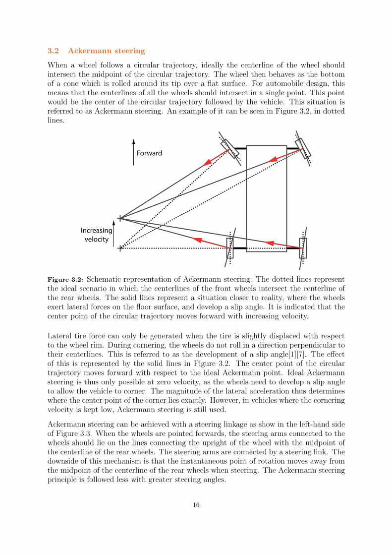
3.2 Ackermann steering

When a wheel follows a circular trajectory, ideally the centerline of the wheel shouldintersect the midpoint of the circular trajectory. The wheel then behaves as the bottomof a cone which is rolled around its tip over a flat surface. For automobile design, thismeans that the centerlines of all the wheels should intersect in a single point. This pointwould be the center of the circular trajectory followed by the vehicle. This situation isreferred to as Ackermann steering. An example of it can be seen in Figure 3.2, in dottedlines.

Forward

Increasing

velocity

Figure 3.2: Schematic representation of Ackermann steering. The dotted lines representthe ideal scenario in which the centerlines of the front wheels intersect the centerline ofthe rear wheels. The solid lines represent a situation closer to reality, where the wheelsexert lateral forces on the floor surface, and develop a slip angle. It is indicated that thecenter point of the circular trajectory moves forward with increasing velocity.

Lateral tire force can only be generated when the tire is slightly displaced with respectto the wheel rim. During cornering, the wheels do not roll in a direction perpendicular totheir centerlines. This is referred to as the development of a slip angle[1][7]. The effectof this is represented by the solid lines in Figure 3.2. The center point of the circulartrajectory moves forward with respect to the ideal Ackermann point. Ideal Ackermannsteering is thus only possible at zero velocity, as the wheels need to develop a slip angleto allow the vehicle to corner. The magnitude of the lateral acceleration thus determineswhere the center point of the corner lies exactly. However, in vehicles where the corneringvelocity is kept low, Ackermann steering is still used.

Ackermann steering can be achieved with a steering linkage as show in the left-hand sideof Figure 3.3. When the wheels are pointed forwards, the steering arms connected to thewheels should lie on the lines connecting the upright of the wheel with the midpoint ofthe centerline of the rear wheels. The steering arms are connected by a steering link. Thedownside of this mechanism is that the instantaneous point of rotation moves away fromthe midpoint of the centerline of the rear wheels when steering. The Ackermann steeringprinciple is followed less with greater steering angles.

16

Steering armsPitman arm

Steering

link Instantaneous

point of rotation

Figure 3.3: Left: Ackermann steering linkage. Right: Ackermann steering linkage withan added pitman arm.

The steering linkage on the left-hand side of the Figure 3.3 offers limited possibilities ofactuating the steering link between the steering arms. In the right hand side of Figure3.3 the steering linkage is complemented with an additional link. This link is called thePitman arm. A rotation point is added around which the Pitman arm can be actuated.

In Figure 3.4 it may be observed that the addition of the Pitman changes the excursions ofthe steering linkage. The instantaneous point of rotation of the linkage with the pitmanarm describes a curve with a broader apex than the linkage without the pitman arm.This means the Ackermann principle is followed more closely by the mechanism with theadded Pitman arm. Furthermore, the Pitman allows for easier actuation of the steeringlinkage.

17

Figure 3.4: Comparison of the movement of the instantaneous point of rotation for thelinkages shown in the left hand side (blue) and right hand side (red) of Figure 3.3

18

3.3 Tire choice

Many indoor AGV’s have wheels with a solid steel wheel hub. Directly on the wheelhub a polyurethane coating is added. Such wheels offer a high load carrying capacity,which is particularly useful for AGV’s that need to carry entire pallets with products.Wheels with polyurethane coatings perform well on floor surfaces with few irregularities.Compared to pneumatic wheels of the same diameter, polyurethane wheels have moremass. This increases the unsprung mass of the AGV, and makes it less useful on floorsurfaces with many irregularities. Next to this, polyurethane wheels cannot generate asmuch traction as pneumatic wheels of the same size. Lastly, a polyurethane wheel needsto be replaced entirely when it is damaged. Pneumatic wheels can often be repaired bychanging the tire. As the order picking robot does not need to carry large payloads,pneumatic wheels are therefore preferred over solid wheels.

Due to the load on the wheel, it will slightly deform, as can be seen in Figure 3.5. Rolling aloaded wheel therefore continually deforms the tire. As deforming the tire takes a certainamount of energy, energy is lost while rolling the wheel. To reduce the amount of energylost, the wheels should either be thin and have a large diameter, or be wide and have asmall diameter [1]. Wheels with a large diameter result in a heavier unsprung mass andhigher torque needed on the drive shaft. Therefore tires with a radius of 150 [mm] anda width of 50 [mm] (6x2 inches) are used. Such tires are predominantly used on smallscooters.

Figure 3.5: Deformation of a loaded wheel. The dotted line indicates the shape of thewheel before loading.

The stiffness of the tire influences the clearance between the AGV and the floor. Thismakes it important input for the design of both the front- and rear wheel suspension.The stiffness of a tire depends on the tire pressure. A typical value for the tire stiffnessof a pneumatic wheel is 170

[Nmm

], at a tire pressure of 2[bar] [8]. While the chosen tires

can be inflated up to 5[bar], this value gives a rough indication for the loss in clearanceusing a pneumatic tire. During acceleration, the load is equal to 570 [N ] per wheel. Theindentation of the tire can now be calculated:

570 [N ]

170[

Nmm

] ≈ 3.5 [mm]

This can be used to determine the necessary clearance between the rear wheel suspensionand the floor.

19

3.4 Wheel construction

The construction of the wheel is shown in Figure 3.6. A hub reinforcement is welded ontoeach half of the wheel hub. These hub reinforcements have internal flats. The flats allowa drive shaft with equally sized flats to transmit torque to the wheel hub. The tube andthe tire are put over the inner wheel hub. The air nipple of the tube is put through holesin the rim of the inner wheel hub as well as the side of the inner wheel hub. The outerwheel hub is then aligned with the inner wheel hub. The air nipple should go throughthe hole in the side of the outer wheel hub. It can then be accessed from the side of thewheel, where it allows for inflation of the inner tire. The inner and outer wheel hub arebolted together using six bolts and nuts. This bolted construction allows for replacementof both the inner and outer tires in case they have been punctured.

Figure 3.6: Construction of the Wheel. 1 : Tire 2 : Tube 3 : Outer wheel hub 4 :

Inner wheel hub 5 : Air nipple 6 : Hub reinforcement 7 : Bolt

20

4 Front wheel suspension

An overview of the front wheel suspension is presented in Figure 4.1. It is based onthe McPherson strut suspension design. This design was chosen for its compactness andstraightforward assembly. A leaf spring is attached to the bottom of the upright with aball joint. Dampers are connected to the upright from the top. The upper part of thedampers should be attached to the frame. The centerlines of the dampers point to theball joints attached to the leaf spring. The piston of the dampers can be freely rotated.This allows the wheels to be steered around the centerline of the damper. A steering armis added to the upright, allowing the steering of the wheel to be actuated. The wheel istherefore constrained in 4 degrees of freedom; only the rotation of the wheel around itsaxis and upward motion of the wheel are free.

Figure 4.1: Front wheel suspension. 1 : Pitman arm 2 : Damper 3 : Steering arm

ball joint 4 : Leaf spring 5 : Upright ball joint 6 : Upright

21

4.1 Construction of the upright

The wheel is attached to the front wheel suspension via the upright, shown in Figure 4.2.The wheel is mounted on an axlestub. A more detailed view of this axlestub is shown inFigure 4.3. The upright contains two deep groove ball bearings, which are positioned atan equal distance from the midline of the wheel hub. As the normal load acting on thewheel is introduced into the axlestub via the hub reinforcements, a moment arises in themiddle of the ball bearing closest to the wheel hub reinforcements. A second ball bearingtherefore needs to be used, as the normal load acting on the wheel would otherwise loadthe ball bearing close to the wheel hub reinforcements unfavorably. The inner races ofthe bearings are kept apart by the bearing spacer. The axlestub rests against the innerrace of the bearing farthest from the hub reinforcements. Another spacer is used to keepthe hub reinforcement and the inner race of the bearing closest to the hub reinforcementapart. The flats of the axlestub are aligned with the flats in the hub reinforcement, anda locknut is put over the end of the axlestub. The inner races of the bearings are herebypulled against the hub reinforcement.

Figure 4.2: Upright. 1 : Locknut 2 : Hub reinforcement 3 : Spacer 4 : Ball bearings

5 : Bearing spacer 6 : Upright

Figure 4.3: Detailed view of the axlestub used in the front wheel

22

4.2 Pitman arm

The pitman arm is placed over the leaf spring. A detailed view of the Pitman arm isshown in Figure 4.4. The Pitman arm is made using a sandwich of two identical partialplastic gears. The ball joints of the rods connected to the steering arms are directlyattached to these gears. The gears are separated by bushes, which also serve as an endstop for the mechanism. This prevents the gears from losing contact with the pinion, ascan be seen in Figure 4.5. The pitman arm is connected to the bottom of the frame ofthe AGV. A motor contained inside of the frame can therefore drive the pinion runningover the partial plastic gears. The Pitman arm is connected to the steering arms withthe steering links. This can be seen in Figure 4.6.

Figure 4.4: Detailed view of the Pitman arm 1 : Partial gear 2 : Driving pinion 3 :

Sandwich plate 4 : Bush/ end stop 5 : Ball of ball joint 6 : Driven axle

Figure 4.5: Excursion of the steering mechanism 1 : Steering arm 2 : Steering link 3 :Bush/ end stop

23

Figure 4.6: Placement of the steering mechanism. The lines extended between the balljoint of the steering arm and the upright intersects the centerline of the rear axle in the

middle 1 : Steering arm 2 : Steering link 3 : Pitman arm

4.3 Leaf spring

A partial view of the assembled leaf spring can be seen in Figure 4.7. The leaf springis attached to the bottom of the frame of the AGV. A block is attached to the free endof the leaf spring. This block is used to attach the cup of a ball joint to the leaf spring.This cup will contain the ball connected to the upright.

Figure 4.7: Assembly of the leaf spring. 1 : Leaf spring 2 : Attachment to frame 3 :Block containing cup of ball joint

Because the AGV drives over irregularities in the floor surface, the leaf spring constantlydeforms elastically. The leaf spring itself is therefore fabricated from a straight strip ofspring steel. This type of steel is used because of its high endurance limit. The leafspring will be attached to the block containing the ball joint and the silent blocks usingpartial holes in the side of the leaf spring. This can be seen in Figure 4.8. Drilling holesinto the leaf spring would result in stress concentrations, which can lead to failure of the

24

spring. When the AGV needs to make an emergency stop, most load is transferred tothe front wheels. In this situation, the leaf spring needs to be perfectly straight. Thehigh longitudinal forces caused by deceleration would otherwise twist the leaf spring, andthus lead to unnecessary stress concentrations. The leaf spring is therefore given a slightradius downwards. The radius should be chosen in such a way that it closely resemblesthe shape of an initially flat leaf spring which is subjected to the normal load on thewheels during full deceleration.

Figure 4.8: Leaf spring curvature.

25

5 Rear wheel suspension

The rear wheel suspension is based on the suspension system of a truck. It features amechanical differential contained in a rigid axle. The axle is mounted to the frame usingan A-frame, two longitudinal struts and two shock absorbers. An overview of the rearwheel suspension can be found in Figure 5.1.

Figure 5.1: Overview of the designed rear wheel suspension. 1 : Strut 2 : A-frame 3 :

Differential housing 4 : Shock absorber

5.1 Rear wheel drive and suspension concepts

A rear wheel suspension housing an electronic differential, a mechanical differential usingNylon gears and a mechanical differential using steel gears are conceptualized in individualsubsections. A concept choice is made using the advantages and disadvantages listed witheach concept.

5.1.1 Electronic differential

In Figure 5.2 a rear wheel drive concept based on an electronic differential is shown. Itfeatures two electric motors independently driving the rear wheels. When the AGV issteered into a corner, the motor controllers should therefore force the electric motors tospin the inside and outside wheels at the correct rotational velocity. The drive shaft iscontained in an axle, and directly connects the wheel to the electric motor. The axle isattached to the AGV using a leaf spring close to the center of the AGV. The axle is also

26

attached to the frame using a longitudinally placed strut. This strut is connected to thebottom of the axle, near the wheels. Together, the leaf spring and the strut constrainlongitudinal motion and rotation around the normal to the floor surface. Rotation aroundthe centerline of the AGV is free, which allows vertical motion of the wheel during a bump.

The electric motors are contained in a thick-walled tube with saw cuts. The saw cutscreate an internal degree of freedom in the tube. When the tube is sandwiched betweenthe leaf springs, the internal degree of freedom of the tube allows the rotation of thewheels around the centerline of the AGV. The thick-walled tube couples the rotationaround the centerline of the AGV of both axles. Therefore, when the normal load on onewheel increases, both wheels move up. The thick-walled tube is attached to an A-frame,above the centerline of the axles. This A-frame constrains the lateral movement of bothwheels. As the A-frame and the struts are attached above and below the axle respectively,they constrain the rotation around the centerline of the axle. The weight of the frame iscarried by shock absorbers. The centerlines of the shock absorbers point at the contactpatch between the wheels and the ground, in order to introduce the normal load actingon the wheels properly into the frame of the AGV.

1 2

7

7

8

89 9

3 4 5 6 12

1 2 5

Figure 5.2: Concept of a rear-wheel drive with an electronic differential. 1 : Wheel 2 :

Axle 3 : Shaft 4 : Leaf spring 5 : Electric motor 6 : Thick-walled tube with saw cut

7 : Shock absorber 8 : A-frame 9 : Strut

27

Employing the described electronic differential concept has the following advantages (+)and disadvantages (−):

+ Independently driving the rear wheels allows for skid steering maneuvers. This canbe used to reduce the minimum cornering radius of the AGV.

+ The thick-walled tube makes sure that the frame does not roll much when load istransferred from one wheel to the other, for example during cornering.

− Because the motion of both axles is coupled with the thick-walled tube, the unsprungmass felt by a single wheel is the total weight of the rear suspension.

− The behavior of the AGV is unpredictable when one of the electric motors fail.

− The size of the electric motor directly influences the clearance between the floor andthe bottom of the AGV.

5.1.2 Mechanical differential using Nylon gears

A mechanical differential can be made out of Nylon gears. Using Nylon gears instead ofsteel gears has the following advantages [9]:

� Nylon gears cost less than steel gears

� No lubrication is needed when Nylon gears are paired with steel pinions

� Nylon gears run more smoothly and more silently compared to steel gears

Nylon is less strong than steel. Therefore it is beneficial to reduce the tooth forces onthe Nylon gear as much as possible. For the gears in the differential, this can be doneby adding a reduction close to the wheels, as can be seen in Figure 5.3. The diameterof the gear of the reduction close to the wheels is constrained by the required clearancebetween the bottom of the AGV and the floor. Taking into account the wheel radius, theindentation of the wheels, and saving room for a housing for the reduction, a referencediameter of Ø65 [mm] is chosen for the gear of the reduction. The tooth forces on thegears will be calculated using the maximum torque during acceleration. As the AGV willnot constantly accelerate during its lifetime, this ensures that the reductions last for theentire lifespan of the AGV. The teeth forces are calculated:

23 [Nm]

0.0325 [m]≈ 710 [N ]

A close estimation of the necessary size of the gear can be made by using the followingequation:

S =

−→F tooth

MBY

In which S is the fatigue stress,−→F tooth is the force on an individual tooth, M is the module

of the gear, B is the width of the gear and Y is the Lewis form factor. The fatigue stressS is a parameter that depends on the material and the estimated amount of load cycles.The design stress for Nylon gears can be determined using the characteristic in Figure5.4. The Lewis form factor depends on the exact shape of the teeth of a gear. For a firstestimation Y should be chosen as 0.6 [9].

28

3 4

1 2

6

5

Figure 5.3: Drivetrain using a Nylon mechanical differential. 1 : Drive shaft 2 : Steel

pinion 3 : Nylon gear 4 : Steel pinion of spur gear differential 5 : Nylon gear of spur

gear differential 6 : Wheel

Figure 5.4: Fatigue stress characteristic of Nylon. The fatigue stress is plotted versus theestimated total amount of load cycles.

29

The Nylon gear is paired with a steel pinion, and does not need continuous lubrication.Therefore the curve for initial lubrication is used. The total amount of wheel rotationsduring the lifetime of the AGV is equal to 40 million. The corresponding fatigue stressis S = 10 [MPa]. As the tooth forces on the Nylon gear are relatively high, a module ofM = 5 [mm] is chosen. The width of the gear can now be calculated:

710

5 · 10 · 0.6≈ 25 [mm]

Choosing a steel pinion with a reference diameter of Ø30 [mm] results in a reduction ofapproximately 1:2. The reduction cannot be made larger as the a module of M = 5 [mm]prohibits the use of a smaller reference diameter of the pinion. With this reduction thetorque on the driving axle is reduced to approximately 12 [Nm]. This is again a worstcase scenario calculation, as the AGV will not accelerate the entire time. It is chosen todesign a spur gear differential. A schematic drawing of such a differential can be seenin Figure 5.5. A spur gear differential is less costly than a bevel gear differential or aTorsen differential. This is because spur gears are easier to manufacture. The drive shaftis located above the wheel axes. This allows for a reference diameter of Ø120 [mm] forthe gears of the spur gear differential. The gears can then be used in combination withpinions having a reference diameter of Ø20 [mm]. The torque is distributed over twopinions. This is in order to balance the differential during its rotation. The tooth forcescan be calculated as follows:

1

2· 12 [Nm]

0.060 [m]≈ 100 [N ]

The gears of the differential rotate 5 million times with respect to each other over thecourse of the AGV’s lifespan. This results in 10 million load cycles because of the useof 2 pinions. As the steel pinions interact with each other, lubrication should be addedto the differential. Because the total amount of load cycles is low compared to the totalamount of wheel rotations, continuous lubrication is not necessary. The fatigue stress istherefore S = 15 [MPa]. A module of M = 1 [mm] is chosen for a smooth operation.The width of the gears in the spur gear differential can now be calculated:

100

1 · 15 · 0.6≈ 10 [mm]

The width of the pinions chosen twice as large. This results in the spur gear differentialshown in Figure 5.5.

A straightforward way of housing the components of the drivetrain is shown in Figure 5.6.Tubes are used to connect the output ends of the reductions with each other. The tubesaround the centerline of the wheels and the centerline of the differential are connected toeach other using plates. Therefore, lateral forces exerted by the wheels on the constructiondo not bend the housing of the reduction. Suspension links connect the reduction housingand the differential housing to the frame of the AGV. An A-frame can be attached tothe top of the differential housing. The A-frame constrains lateral motion of the housing.Struts are attached to the bottom of the tube around the wheel centerline. The strutsconstrain the rotation around the normal to the floor. Together, the struts and the A-frame constrain longitudinal motion and the rotation around the centerline of the wheels.Vertical motion, and rotation around the centerline of the AGV are left free.

30

reference diameter pinion: Ø20 mm

reference diameter gear: Ø120 mm

width gear: 10 mm

width pinion: 20 mm

Figure 5.5: Schematic drawing of the designed Nylon spur gear differential

1 3 4

5

2

1

2

1

27

7

7

5

6

6

6

Figure 5.6: Housing for the Nylon reduction and spur gear differential. 1 : Reduc-

tion housing 2 : Differential housing 3 : Plate 4 : Drive shaft centerline 5 : Wheel

centerline 6 : Strut 7 : A-frame

31

Employing the concept of a mechanical differential made using Nylon gears has the fol-lowing advantages (+) and disadvantages (−):

+ The differential could be driven with a chain or a belt. Because of the large diameterof the differential, and the reduction close to the wheels, a small sprocket attachedto the driving motor results in a large reduction between the motor and the wheels.Therefore expensive gear sets do not have to be installed on the driving motor.

+ Moving the drive shaft upwards using the reduction at the wheels results in a largeclearance between the floor and the bottom of the AGV.

− The complex shape of the differential housing and the reduction housing makes theconcept costly.

− The size of the housing will result in a large unsprung mass.

5.1.3 Mechanical differential using Steel gears

A mechanical differential can also be made using steel gears. Steel is strong enough toallow for the direct connection of the drive shafts to the gears of the spur gear differential.A concept featuring such a drivetrain is visualized in Figure 5.7. The differential and thedrive shafts are enveloped in the axle. An A-frame and two struts are used to connectthe axle to the frame. Together they constrain the axle in four degrees of freedom; onlyvertical motion and rotation around the centerline of the AGV are left free. Two shockabsorbers are used to carry the weight of the frame.

The fatigue stress characteristic of steel remains constant above a certain amount ofcycles. This is referred to as the endurance limit. Using the endurance limit, a differentialcan be designed which could in theory remain operational forever. Unhardened mild steelspur gears are used to construct a spur gear differential. The endurance limit of mildsteel is approximately 200 [MPa].

Keeping the indentation of the wheels and the minimum clearance between the bottom ofthe AGV and the floor into account, the maximum diameter of the axle can be Ø80 [mm].Saving room for a differential housing, the reference diameter of the gear is chosen to beØ40 [mm]. The reference diameter of the pinions is chosen to be Ø15 [mm]. The torqueon the drive shafts is distributed over two pairs of meshing teeth, as there are two pinionson the circumference of the gear. The maximum tooth forces can now be calculated:

1

2· 23 [Nm]

0.020 [m]≈ 580 [N ]

Choosing a module of M = 1 [mm], the width of the gears can now be calculated. Thewidth of the pinions is chosen twice as large as the width of the gears.

580

1 · 200 · 0.6≈ 5 [mm]

A schematic drawing of the resulting spur gear differential can be seen in Figure 5.8. Thespur gear differential fits within a diameter of Ø72 [mm]. This leaves enough room forfitting a differential housing within the axle.

32

1 2 3 4

5

12

76 6

Figure 5.7: Drivetrain using a mechanical differential made out of steel, and corresponding

suspension design. 1 : Wheel 2 : Axle 3 : Drive shaft 4 : Steel spur gear differential

5 : Shock absorber 6 : Strut 7 : A-frame

reference diameter gear: Ø40 mm

reference diameter pinion: Ø15 mm

width gear: 5 mm

width pinion: 10 mm

Figure 5.8: Schematic drawing of the designed steel spur gear differential

33

Employing the concept of a mechanical differential made using steel gears has the follow-ing advantages (+) and disadvantages (−):

+ The differential has a practically infinite lifetime.

+ The unsprung mass is low compared to the other concepts.

− There is little clearance between the bottom of the AGV and the floor.

5.1.4 Concept choice

The concept with the steel mechanical differential is chosen over the other concepts. Itcan be built lightweight in comparison with the other concepts. The electronic differentialoffers extra maneuverability due to the possibility of skid steering, but this is not necessaryas the robotic arm omits the need for more accurate positioning of the AGV. For theconcept with the steel differential, this can be improved by choosing stiffer springs. Havinga large reduction between the driving motor and the wheels, which can be achieved withthe Nylon spur gear differential concept, is less beneficial than a low unsprung mass. Asthe concept with the Nylon spur gear differential has a large unsprung mass due to thesize of the differential housing, it is therefore not suitable for the design of the AGV. Theconcept with the steel differential has a low clearance between the bottom of the AGVand the floor. However, calculations show that it is possible to maintain the minimumclearance while providing enough room for the differential.

5.2 Differential construction

The differential is constructed according to Figure 5.9. The differential housing containstwo Nylon covers on either side of the differential itself. These covers have a center hole toaccommodate the drive shaft. The cover also contains halfway holes in which the pinionaxles rest. Spacers make sure that the pinions stay on the correct side of the differential.

By choosing a self-lubricating Nylon the covers can also serve as plain bearings for thedrive shafts and the pinion axles. The covers are glued into the differential housing toavoid lubricant from escaping. Two indentations are made in the differential housingon either side of the Nylon covers upon assembly. It is therefore possible to transmittorque from the sprocket, through the housing, to the Nylon covers. The torque is thentransmitted through the plain bearings, into the pinion axles, and into the pinions. Flatsare ground onto the drive shafts to allow them to transfer torque to the wheels. The endsof the shafts also have thread to allow a locknut to be mounted on the shafts.

An aligning pin is added between the two driving shafts. This pin makes sure that themeshing of the gears remains straight. Holes are bored axially into the drive shafts. Theseholes contain needle bearings that guide the aligning pin. Drawn cup needle bearings arechosen for their high loading capacity, compact size and low price.

34

Figure 5.9: Figure 1: Construction of the differential plus housing. 1 : Drive shaft with

flats 2 : Nylon cover 3 : Differential housing 4 : Indentation in the plastic cover/

differential housing 5 : Gear 6 : Pinion 7 : Spacer 8 : Pinion axle 9 : Aligning pin

10 : Needle bearing 11 : Sprocket

5.3 Axle assembly

In Figure 5.10 a section view of the rear axle is shown. The axle consists of two partswhich can be bolted together using flanges. Circlips are added to the drive shafts. Thedrive shafts are put through deep-groove ball bearings which are contained within theaxles, close to the wheels. Deep groove ball bearings can handle lateral forces, and arelower in cost compared to angular contact ball bearings. Next to this the mountingtolerances for deep-groove ball bearings are less critical than for angular contact ballbearings. A spacer is added over the drive shaft, whereafter the wheel hub is alignedwith the flats on the shaft. Using a locknut, the inner race of the ball bearing is pulledagainst the spacer, which rests against the wheelhub. Lateral forces from the wheelsin either direction can now be transmitted through the ball bearing. The ball bearinglies exactly on the midline of the wheel. This ensures that vertical forces are correctlyintroduced into the ball bearing. The ball bearing transmits the wheels forces into theaxle, where the suspension links and the shock absorbers can transmit them into theframe.

Flanges are attached to both halves of the axle. A schematic view of these flanges canbe seen in Figure 5.11. The flanges can be cut from a plate, and welded to the individualaxle halves. When the drive shafts and the differential are assembled in the axle, theflanges are bolted together, joining both axle halves together.

In Figure 5.13 the mounting points for the struts and the A-frame are shown. Mounts forthe struts could be directly attached to the individual halves of the axle. However, thiswould result in strict tolerances for the individual axle halves, as an offset strut mount

35

Figure 5.10: Section view of the rear axle. 1 : Drive shaft 2 : Deep groove ball bearing

3 : Spacer 4 : Hub reinforcement 5 : Locknut 6 : Differential 7 : Flange 8 : A-frame mount

Figure 5.11: Flange mounted onboth axle halves.

Figure 5.12: Mounting clamp forthe struts.

Figure 5.13: Mounting points for the strut and the A-frame on the axle. 1 : Strut clamp

2 : Strut 3 : Bolt 4 : Silent block bracket 5 : Outer tube of silent block 6 : Inner

tube of silent block 7 : Vulcanized rubber between the inner and outer tube of the silent

block 8 : A-frame 9 : Bolt 10 : Nut

36

could hinder the suspension travel. Strict tolerances would also make the production ofthe axle halves more expensive. Therefore clamps are used to attach the struts to theaxle. Such a clamp is shown in detail in Figure 5.12. The axle runs through the largecentral hole of the clamp, and a bolt is screwed into the clamp to tighten it around theaxle. A strut can be attached to the clamp using a bolt. The A-frame is mounted to theaxle by use of a silent block. A silent block consists of an inner and an outer tube withvulcanized rubber in between. It offers some damping, as well as minor rotations of theinner tube with respect to the outer tube in three directions (≤ 5◦). Both halves of theA-frame are attached to the silent block using a bolt and a nut.

5.4 Construction of the A-frame and the struts

The struts and the A-frame are fabricated by bending strips in a U-shape, and welding astraight strip inside, as can be seen in Figure 5.14. For the A-frame, also angled insertsare welded in both ends of the tube to allow the halves of the A-frame to be attached tothe axle under an angle. The struts are created in a similar fashion, the only differencebeing that no inserts are welded into them. Because the ends of the struts are left open,they are torsionally compliant. This is necessary in order to allow for the rotation of theaxle around the centerline of the AGV.

Figure 5.14: Construction of one half of the A-frame. 1 : Bent strip 2 : Straight strip

3 : Angled insert

37

6 Conclusion

A front- and rear wheel suspension design was made for an AGV that needs to supportan order picking robot. Both front- and rear wheel suspension are designed to enable theAGV to corner faster than the current AGV allows the order picking robot to, and to bemore robust to irregularities in the floor surface. Next to this, cost effectiveness for theproduction of components and assembly of the AGV is taken into account.

The new AGV has rear wheels drive, and front wheel steering. Separating the actuationfor driving and steering decouples the motion control of the AGV. This makes it easierto maintain velocity during cornering. The steering is based on an Ackermann steeringlinkage. Pneumatic wheels are used on the AGV, which are lighter than commonly usedpolyurethane wheels. The wheel hubs have been constructed so they can be used bothas front and rear wheels. This decreases the component count of the AGV.

The front wheel suspension is based on a McPherson strut suspension design. The wheelsare connected to an upright which has two deep-groove ball bearings supporting thewheels. The upright is attached to a damper connected to the frame, and to a balljoint attached to a leaf spring. Because the piston of the damper can freely rotate in itshousing, the wheel can be steered around the centerline of the damper. The leaf springis mounted to the frame. The pitman arm consists of two identical partial gears runningagainst a pinion that can be actuated from within the frame. The gears and the pinionsare sandwiched between two plates, to close the force loop. The pitman arm is connectedto the steering arms by the steering links.

Different drivetrain concepts have been analyzed and compared. A drive train using amechanical differential made with steel gears is most beneficial. The differential and itshousing are contained in the axle. The differential is directly connected to the wheels withtubular shafts. The suspension is based on the suspension design of a truck; an A-frameis attached to the top of the axle, and two longitudinally placed struts are mounted tothe bottom of the axle close to the wheels. The weight of the frame is carried by twoshock absorbers.

7 Recommendations

An improved wheel model should be used to more accurately predict the forces that thewheels can exert on the road. Using such a model the design for the front- and rear wheelsuspension can be finalized. A suggestion for such a model is the Magic Formula [10].This model relies on experimental data, and therefore wheel tests should be carried outas well.

Instead of focusing on the order picking robot, different concepts should also be analyzed.The racks of the warehouse could be adapted in such a way that they can drop itemsone by one, instead of a worker or a robot having to pick an item from the totes. Thissimplifies the design of the AGV, as it only has to carry a tote to ’catch’ the items fallingfrom the racks. The AGV can thus be much lighter, and operate longer on a singlecharge. The picking time could even be reduced to zero by dropping an item from therack just in time for the AGV to catch it. To still allow order pickers in the warehouse,each rack could feature buttons which trigger an item to drop. Warehouse managementtherefore also becomes much more efficient, as the robot and the order picker use thesame mechanism.

38

References

[1] P. Brinkgreve, R. Brinkgreve, M. J. M. van der Velden: Wegligging van Automo-bielen, 1969-1972

[2] J. L. Blanco, M. Bellone and A. Gimenez-Fernandez: TP-Space RRT KinematicPath Planning of Non-Holonomic Any-Shape Vehicles, 2015

[3] J. Ackermann, J. Guldner, W. Sienel, R. Steinhauser, and V. I. Utkin: Linear andNonlinear Controller Design for Robust Automatic Steering, 1995

[4] T. Fraichard and J. M. Ahuactzin: Smooth Path Planning for Cars, 2001

[5] D. Dolgov: Path Planning for Autonomous Vehicles in Unknown Semi-structuredEnvironments, 2010

[6] G. A. den Boer, G. D. van Albada, L. O. Hertzberger, C. Koburg and M. Mergel:The MARIE autonomous mobile robot, 1993

[7] I. J. M. Besselink: Lecture notes vehicle dynamics, 2016

[8] J. Reimpell, H. Stoll, J. W. Betzler: The automotive chassis: engineering principles,2001

[9] C. E. Adams: Plastic gearing: selection and application, 1986

[10] H. B. Pacejka: Tyre and vehicle dynamics, 2002

39